Feedback Control Systems ( FCS )

Feedback Control Systems (FCS)

Dr. Imtiaz Hussainemail: [email protected]

URL :http://imtiazhussainkalwar.weebly.com/

Lecture-22-23-24 Time Domain Analysis of 2nd Order Systems

mailto:[email protected]

Introduction• We have already discussed the affect of location of poles and zeros on

the transient response of 1st order systems.

• Compared to the simplicity of a first-order system, a second-order system exhibits a wide range of responses that must be analyzed and described.

• Varying a first-order system's parameter (T, K) simply changes the speed and offset of the response

• Whereas, changes in the parameters of a second-order system can change the form of the response.

• A second-order system can display characteristics much like a first-order system or, depending on component values, display damped or pure oscillations for its transient response.

Introduction• A general second-order system is characterized by

the following transfer function.

22

2

2 nn

n

sssRsC

)(

)(

Introduction

un-damped natural frequency of the second order system, which is the frequency of oscillation of the system without damping.

22

2

2 nn

n

sssRsC

)(

)(

n

damping ratio of the second order system, which is a measure of the degree of resistance to change in the system output.

Example#1

424

2

sssRsC)()(

• Determine the un-damped natural frequency and damping ratio of the following second order system.

42 n

22

2

2 nn

n

sssRsC

)(

)(

• Compare the numerator and denominator of the given transfer function with the general 2nd order transfer function.

sec/radn 2 ssn 22

422 222 ssss nn 50. 1 n

Introduction

22

2

2 nn

n

sssRsC

)(

)(

• Two poles of the system are

1

12

2

nn

nn

Introduction

• According the value of , a second-order system can be set into one of the four categories:

1

12

2

nn

nn

1. Overdamped - when the system has two real distinct poles ( >1).

-a-b-cδ

jω

Introduction


1

12

2

nn

nn

2. Underdamped - when the system has two complex conjugate poles (0 < <1)

-a-b-cδ

jω

Introduction


1

12

2

nn

nn

3. Undamped - when the system has two imaginary poles ( = 0).

-a-b-cδ

jω

Introduction


1

12

2

nn

nn

4. Critically damped - when the system has two real but equal poles ( = 1).

-a-b-cδ

jω

Time-Domain Specification

11

For 0< <1 and ωn > 0, the 2nd order system’s response due to a unit step input looks like


12

• The delay (td) time is the time required for the response to reach half the final value the very first time.


13

• The rise time is the time required for the response to rise from 10% to 90%, 5% to 95%, or 0% to 100% of its final value.

• For underdamped second order systems, the 0% to 100% rise time is normally used. For overdamped systems, the 10% to 90% rise time is commonly used.

13


14

• The peak time is the time required for the response to reach the first peak of the overshoot.

1414


15

The maximum overshoot is the maximum peak value of the response curve measured from unity. If the final steady-state value of the response differs from unity, then it is common to use the maximum percent overshoot. It is defined by

The amount of the maximum (percent) overshoot directly indicates the relative stability of the system.


16

• The settling time is the time required for the response curve to reach and stay within a range about the final value of size specified by absolute percentage of the final value (usually 2% or 5%).

S-Plane

δ

jω

• Natural Undamped Frequency.

n

• Distance from the origin of s-plane to pole is natural undamped frequency in rad/sec.

S-Plane

δ

jω

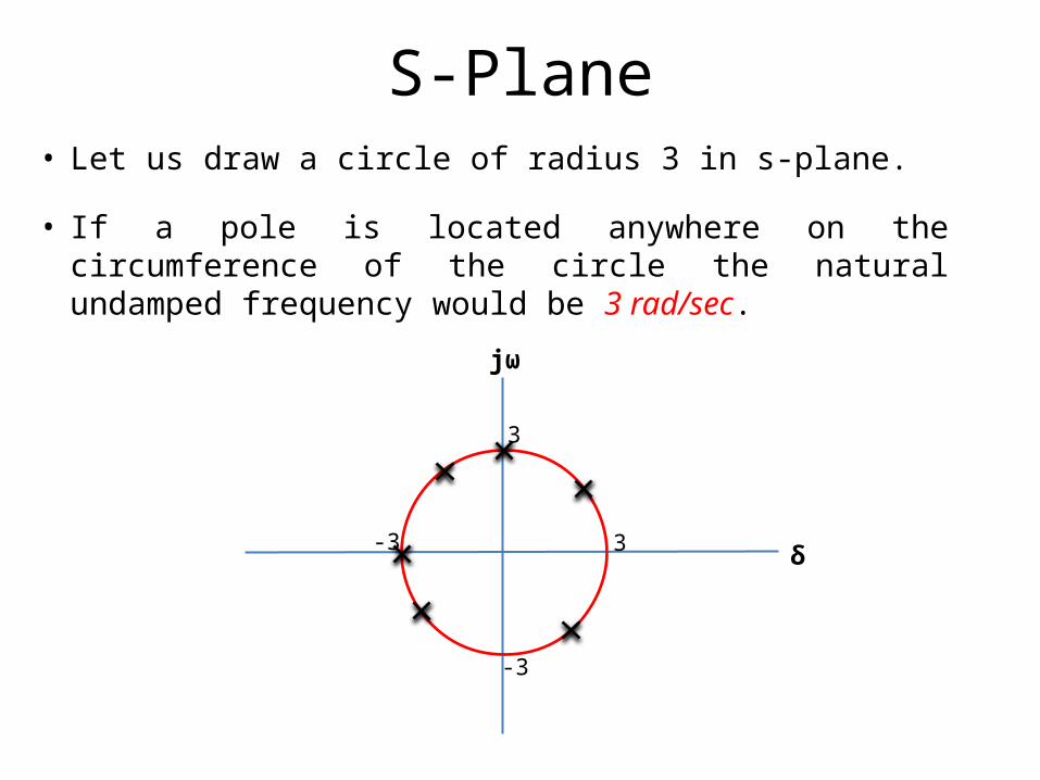
• Let us draw a circle of radius 3 in s-plane.

3

-3

-3

3

• If a pole is located anywhere on the circumference of the circle the natural undamped frequency would be 3 rad/sec.

S-Plane

δ

jω

• Therefore the s-plane is divided into Constant Natural Undamped Frequency (ωn) Circles.

S-Plane

δ

jω

• Damping ratio.

• Cosine of the angle between vector connecting origin and pole and –ve real axis yields damping ratio.

cos

S-Plane

δ

jω

• For Underdamped system therefore, 900 10

S-Plane

δ

jω

• For Undamped system therefore, 90 0

S-Plane

δ

jω

• For overdamped and critically damped systems therefore,

00

S-Plane

δ

jω

• Draw a vector connecting origin of s-plane and some point P.

P

45

707045 .cos

S-Plane

δ

jω

• Therefore, s-plane is divided into sections of constant damping ratio lines.

Example-2• Determine the natural frequency and damping ratio of the poles from the

following pz-map.

-4 -3.5 -3 -2.5 -2 -1.5 -1 -0.5 0-1.5

-1

-0.5

0

0.5

1

1.50.220.420.60.740.840.91

0.96

0.99

0.220.420.60.740.840.91

0.96

0.99

0.511.522.533.54

Pole-Zero Map

Real Axis (seconds-1)

Imag

inar

y Ax

is (s

econ

ds-1

)

Example-3

• Determine the natural frequency and damping ratio of the poles from the given pz-map.

• Also determine the transfer function of the system and state whether system is underdamped, overdamped, undamped or critically damped.

-3 -2.5 -2 -1.5 -1 -0.5 0 0.5 1 1.5 2-3

-2

-1

0

1

2

3

0.420.560.7

0.82

0.91

0.975

0.5

1

1.5

2

2.5

3

0.5

1

1.5

2

2.5

3

0.140.280.420.560.7

0.82

0.91

0.975

0.140.28

Pole-Zero Map

Real Axis (seconds-1)

Imag

inar

y Ax

is (s

econ

ds-1

)

Example-4

• The natural frequency of closed loop poles of 2nd order system is 2 rad/sec and damping ratio is 0.5.

• Determine the location of closed loop poles so that the damping ratio remains same but the natural undamped frequency is doubled.

424

2 222

2

sssssRsC

nn

n

)()(

-2 -1.5 -1 -0.5 0 0.5 1-3

-2

-1

0

1

2

3

0.280.380.5

0.64

0.8

0.94

0.5

1

1.5

2

2.5

3

0.5

1

1.5

2

2.5

3

0.080.170.280.380.5

0.64

0.8

0.94

0.080.17

Pole-Zero Map

Real Axis

Imag

inar

y Ax

is

Example-4• Determine the location of closed loop poles so that the damping ratio remains same

but the natural undamped frequency is doubled.

-8 -6 -4 -2 0 2 4-5

-4

-3

-2

-1

0

1

2

3

4

5

0.5

0.5

24

Pole-Zero Map

Real Axis

Imag

inar

y Ax

is

S-Plane

1

12

2

nn

nn

Step Response of underdamped System

222222 221

nnnn

n

sss

ssC

)(

• The partial fraction expansion of above equation is given as

22 221

nn

n

sss

ssC

)(

22 ns

22 1 n

222 1

21

nn

n

s

ss

sC )(

22

2

2 nn

n

sssRsC

)(

)( 22

2

2 nn

n

ssssC

)(Step Response


• Above equation can be written as

222 1

21

nn

n

s

ss

sC )(

2221

dn

n

s

ss

sC

)(

21 nd• Where , is the frequency of transient oscillations and is called damped natural frequency.

• The inverse Laplace transform of above equation can be obtained easily if C(s) is written in the following form:

22221

dn

n

dn

n

ss

ss

sC

)(


22221

dn

n

dn

n

ss

ss

sC

)(

22

2

2

22

111

dn

n

dn

n

ss

ss

sC

)(

222221

1

dn

d

dn

n

ss

ss

sC

)(

tetetc dt

dt nn

sincos)(

211


tetetc dt

dt nn

sincos)(

211

ttetc dd

tn

sincos)(21

1

n

nd

21

• When 0

ttc ncos)( 1


ttetc dd

tn

sincos)(21

1

sec/. radn and if 310

0 2 4 6 8 100

0.2

0.4

0.6

0.8

1

1.2

1.4

1.6

1.8


ttetc dd

tn

sincos)(21

1


0 2 4 6 8 100

0.2

0.4

0.6

0.8

1

1.2

1.4


ttetc dd

tn

sincos)(21

1


0 2 4 6 8 100

0.2

0.4

0.6

0.8

1

1.2

1.4


0 1 2 3 4 5 6 7 8 9 100

0.2

0.4

0.6

0.8

1

1.2

1.4

1.6

1.8

2

b=0b=0.2b=0.4b=0.6b=0.9


0 1 2 3 4 5 6 7 8 9 100

0.2

0.4

0.6

0.8

1

1.2

1.4

wn=0.5wn=1wn=1.5wn=2wn=2.5

Time Domain Specifications of Underdamped system

Time Domain Specifications (Rise Time)

ttetc dd

tn

sincos)(21

1

equation above in Put rtt

rdrdt

r ttetc rn

sincos)(21

1

1)c(tr Where

rdrdt tte rn

sincos21

0

0 rnte

rdrd tt

sincos21

0


as writen-re be can equation above

01 2

rdrd tt

sincos

rdrd tt

cossin21

21

rd ttan

2

1 1tanrd t


2

1 1tanrd t

n

n

drt

21 11 tan

drt

ba1tan

Time Domain Specifications (Peak Time)

ttetc dd

tn

sincos)(21

1

• In order to find peak time let us differentiate above equation w.r.t t.

ttette

dttdc

dd

ddt

ddt

nnn

cossinsincos)(22 11

tttte d

dddd

ndn

tn

cossinsincos

22

2

110

tttte d

nddd

ndn

tn

cossinsincos

2

2

2

2

1

1

10


tttte d

nddd

ndn

tn

cossinsincos

2

2

2

2

1

1

10

01 2

2

tte dddntn

sinsin

0 tne 01 2

2

tt ddd

n

sinsin

01 2

2

d

nd t

sin


01 2

2

d

nd t

sin

01 2

2

d

n

0tdsin

01sintd

dt

,,, 20

• Since for underdamped stable systems first peak is maximum peak therefore,

dpt

Time Domain Specifications (Maximum Overshoot)

pdpdt

p ttetc pn

sincos)(21

1

1)(c

10011

12

pdpdt

p tteM pn

sincos

equation above in Putd

pt

1001 2

dd

ddp

dn

eM

sincos

Time Domain Specifications (Maximum Overshoot)

1001 2

dd

ddp

dn

eM

sincos

1001 2

1 2

sincosnn

eM p

1000121

eM p

10021

eM p

equation above in Put 21-ζωω nd

Time Domain Specifications (Settling Time)

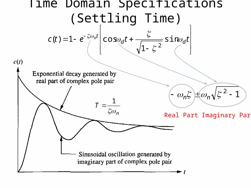
ttetc dd

tn

sincos)(21

1

12 nn

nT

1

Real Part Imaginary Part

Time Domain Specifications (Settling Time)

nT

1

• Settling time (2%) criterion• Time consumed in exponential decay up to 98% of the input.

ns Tt

44

• Settling time (5%) criterion• Time consumed in exponential decay up to 95% of the input.

ns Tt

33

Summary of Time Domain Specifications

ns Tt

44

ns Tt

33 100

21

eM p

21

ndpt

21

ndrt

Rise Time Peak Time

Settling Time (2%)

Settling Time (4%)

Maximum Overshoot

Example#5• Consider the system shown in following figure, where

damping ratio is 0.6 and natural undamped frequency is 5 rad/sec. Obtain the rise time tr, peak time tp, maximum overshoot Mp, and settling time 2% and 5% criterion ts when the system is subjected to a unit-step input.

Example#5

ns Tt

44

10021

eM p

dpt

drt

Rise Time Peak Time

Settling Time (2%) Maximum Overshoot

ns Tt

33

Settling Time (4%)

Example#5

drt

Rise Time

21

1413

n

rt.

rad 9301 2

1 .)(tan

n

n

str 5506015

93014132

....

Example#5

nst

4

dpt

Peak Time Settling Time (2%)

nst

3

Settling Time (4%)

st p 785041413 ..

sts 331

5604 ..

sts 1560

3

.

Example#5

10021

eM p

Maximum Overshoot

1002601

601413

...

eM p

1000950 .pM

%.59pM

Example#5Step Response

Time (sec)

Ampl

itude

0 0.2 0.4 0.6 0.8 1 1.2 1.4 1.60

0.2

0.4

0.6

0.8

1

1.2

1.4

Mp

Rise Time

Example#6• For the system shown in Figure-(a), determine the values of gain K

and velocity-feedback constant Kh so that the maximum overshoot in the unit-step response is 0.2 and the peak time is 1 sec. With these values of K and Kh, obtain the rise time and settling time. Assume that J=1 kg-m2 and B=1 N-m/rad/sec.

Example#6

Example#6

Nm/rad/sec and Since 11 2 BkgmJ

KsKKsK

sRsC

h

)()()(

12

22

2

2 nn

n

sssRsC

)(

)(

• Comparing above T.F with general 2nd order T.F

Kn KKKh21 )(

Example#6

• Maximum overshoot is 0.2.

Kn KKKh21 )(

2021 .ln)ln(

e

• The peak time is 1 sec

dpt

245601

1413

..

n

21

14131

n

.

533.n

Example#6

Kn KKKh21 )(

963.n

K533.

512

533 2

.

.

K

K

).(.. hK512151224560

1780.hK

Example#6963.n

nst

4

nst

3

21

n

rt

str 650. sts 482.

sts 861.

Example#7When the system shown in Figure(a) is subjected to a unit-step input, the system output responds as shown in Figure(b). Determine the values of a and c from the response curve.

)( 1cssa

Example#8Figure (a) shows a mechanical vibratory system. When 2 lb of force (step input) is applied to the system, the mass oscillates, as shown in Figure (b). Determine m, b, and k of the system from this response curve.

Example#9Given the system shown in following figure, find J and D to yield 20% overshoot and a settling time of 2 seconds for a step input of torque T(t).

Example#9

Example#9

Step Response of critically damped System ( )

• The partial fraction expansion of above equation is given as

22

n

n

ssRsC

)(

)( 2

2

n

n

sssC

)(Step Response

22

2

nnn

n

sC

sB

sA

ss

211

n

n

n ssssC

)(

teetc tn

t nn 1)(

tetc ntn 11)(

1

Step Response of overdamped and undamped Systems

• Home Work

71

72

Example 10: Describe the nature of the second-order system response via the value of the damping ratio for the systems with transfer function

Second – Order System

12812)(.1 2

ss

sG

16816)(.2 2

ss

sG

20820)(.3 2

ss

sG

Do them as your own revision

END OF LECTURES-22-23-24

To download this lecture visithttp://imtiazhussainkalwar.weebly.com/

http://imtiazhussainkalwar.weebly.com/

Date post:	23-Feb-2016
Category:	Documents
Upload:	junius
View:	35 times
Download:	0 times

Feedback Control Systems ( FCS )

Documents