Feedback Real-Time Optimization Strategy Using a Novel Steady-state Gradient Estimate and Transient MeasurementsDinesh Krishnamoorthy, Esmaeil Jahanshahi, and Sigurd Skogestad*
Department of Chemical Engineering, Norwegian University of Science and Technology (NTNU), Trondheim, Norway
ABSTRACT: This paper presents a new feedback real-timeoptimization (RTO) strategy for steady-state optimizationthat directly uses transient measurements. The proposed RTOscheme is based on controlling the estimated steady-stategradient of the cost function using feedback. The steady-stategradient is estimated using a novel method based onlinearizing a nonlinear dynamic model around the currentoperating point. The gradient is controlled to zero usingstandard feedback controllers, for example, a PI-controller. Inthe case of disturbances, the proposed method is able toadjust quickly to the new optimal operation. The advantage ofthe proposed feedback RTO strategy compared to standardsteady-state real-time optimization is that it reaches the optimum much faster and without the need to wait for steady-state toupdate the model. The advantage, compared to dynamic RTO and the closely related economic NMPC, is that thecomputational cost is considerably reduced and the tuning is simpler. Finally, it is significantly faster than classical extremum-seeking control and does not require the measurement of the cost function and additional process excitation.
■ INTRODUCTIONReal-time optimization is traditionally based on rigoroussteady-state process models that are used by a numericaloptimization solver to compute the optimal inputs and setpoints. The optimization problem needs to be resolved everytime a disturbance occurs. This step is also know as ”datareconciliation”. Since steady-state process models are used, it isnecessary to wait so that the plant has settled to a new steady-state before updating the model parameters and estimating thedisturbances. It was noted by Darby et al.1 that this steady-statewait time is one of the fundamental limitations of thetraditional RTO approach.In the past two decades or so, there have been developments
on several alternatives to the traditional RTO. A goodclassification and overview of the different RTO schemes isfound in Chachuat et al.,2 Francois et al.,3 and the referencestherein. Recently, to address the problem of the steady-statewait time associated with the traditional steady-state RTO, ahybrid RTO (HRTO) approach was proposed by Krishna-moorthy et al.4 Here, the model adaptation is done using adynamic model and transient measurements, whereas theoptimization is performed using a static model. The HRTOapproach thus requires solving a numerical optimizationproblem in order to compute the optimal set points. It alsorequires regular maintenance of both the dynamic model andits static counterpart.With the recent surge of developments in the so-called direct
input adaptation methods, where the optimization problem isconverted to a feedback control problem,2,3 we here propose toconvert the HRTO strategy proposed by Krishnamoorthy etal.4 into a feedback steady-state RTO strategy. This is based on
the principle that optimal operation can be achieved bycontrolling the estimated steady-state gradient from the inputsto the cost at a constant set point of zero. The proposedmethod involves a novel nonobvious method for estimating thesteady-state gradient by linearizing a nonlinear dynamic model,which is updated using transient measurements. To be morespecific, the nonlinear dynamic model is used to estimate thestates and parameters by means of a dynamic estimationscheme in the same fashion as in the HRTO and dynamicRTO (DRTO) approaches. However, instead of using theupdated model in an optimization problem, the state and theparameter estimates are used to linearize the updated dynamicmodel from the inputs to the cost. This linearized dynamicmodel is then used to obtain the mentioned nonobviousestimate of the steady-state gradient at the current operatingpoint (Theorem 1). Optimal operation is achieved bycontrolling the estimated steady-state gradient to constant setpoint of zero by any feedback controller.The concept of achieving optimal operation by keeping a
particular variable at a constant set point is also the idea behindself-optimizing control, which is another direct inputadaptation method; see Skogestad5 and Jaschke et al.6 It wasalso noted by Skogestad5 that the ideal self-optimizing variablewould be the steady-state gradient from the cost to the input,which when kept constant at a set point of zero, leads tooptimal operation (thereby satisfying the necessary condition
Received: July 10, 2018Revised: October 2, 2018Accepted: December 2, 2018Published: December 3, 2018
for optimality). This complements the idea behind ourproposed method.The concept of estimating and driving the steady-state cost
gradients to zero is also the same as that used in methods suchas extremum-seeking control,7,8 necessary-conditions ofoptimality (NCO) tracking controllers,9 and “hill-climbing”controllers.10 However, these methods are model-free andhence require additional perturbations for accurate gradientestimation. The main disadvantages of such methods are thatthey require the cost to be measured directly and generally giveprohibitively slow convergence to the optimum.11,12
The main contribution of this paper is a novel gradientestimation method (Theorem 1), which is used in a feedback-based RTO strategy using transient measurements. Theproposed method is demonstrated using a CSTR case study.The proposed method is compared with the traditional SRTO(SRTO), DRTO, and the newer HRTO approach. It is alsocompared with two direct-input adaptation methods, namely,self-optimizing control and extremum-seeking control.
■ PROPOSED METHODIn this section, we present the feedback steady-state RTOstrategy. Consider a continuous-time nonlinear process:
=
=
t t t
t t t
x f x u d
y h x u
( ( ), ( ), ( ))
( ) ( ( ), ( )) (1)
where ∈x nx, ∈u nu, and ∈y ny are the states, processinputs, and process measurements, respectively. ∈d nd is theset of process disturbances. × × →f: n n n nx u d x de-scribes the differential equations, and the measurement modelis given by × →h: n n nx u y. Let the cost that has to beoptimized × →J: n nx u be given by
=J t t tg x u( ) ( ( ), ( )) (2)
The measurement model and the cost function are not directlyaffected by the disturbances but are affected via the states.According to the plantwide control procedure,5 we also assumethat any active constraints are tightly regulated and that the nudegrees of freedom considered here are the remainingunconstrained degrees of freedom available for optimization.Assumption 1. Equation 2 is suf f iciently continuous and
twice dif ferentiable, such that for any d eq 2 has a minimum at u= u*. According to the Karush−Kuhn−Tucker (KKT) conditions,the following then hold:
∂
∂∂
* = * =
∂ * = * ≥
uJ
J
u d J u d
uu d J u d
( , ) ( , ) 0 (3)
( , ) ( , ) 0 (4)
u
uu
2
2 (3)
Without loss of generality, we can assume that the optimizationproblem is a minimization problem.The optimization problem can be converted to a feedback
control problem by controlling the steady-state gradient Ju to aconstant set point of Ju
sp = 0. The main challenge is then toestimate the steady-state gradient efficiently. There are manydifferent data-based gradient estimation algorithms thatestimate the steady-state gradient using steady-state measure-ments; see Srinivasan et al.13 In this paper, we propose toestimate the steady-state gradient using a nonlinear dynamicmodel and the process measurements ymeas by means of a
combined state and parameter estimation framework. In thisway, we can estimate the exact gradients around the currentoperating point.Any state estimation scheme may be used to estimate the
states x and the unmeasured disturbances d using the dynamicmodel of the plant and the measurements ymeas. In this paper,for the sake of demonstration, we use an augmented extendedKalman filter (EKF) for combined state and parameterestimation; see Simon14 for detailed description of theextended Kalman filter.Once the states and unmeasured disturbances are estimated,
eq 2 is linearized to obtain a local linear dynamic model fromthe inputs u to the objective function J. Let x (t), u(t), and d(t)denote the original dynamic trajectory that would result if wekeep u unchanged (i.e., no control). Let Δu(t) represent theadditional control input and Δx(t) the resulting change in thestates:
= + Δ
= + Δ
= + Δ
t t t
t t t
t t t
x x x
u u u
d d d
( ) ( ) ( )
( ) ( ) ( )
( ) ( ) ( ) (5)
where we assume u(t) = u(t0) (constant) and d(t) = d(t0)(constant), and t0 denotes the current time. Δd(t) = 0 becausethe control input does not affect the disturbances. For controlpurposes, the local linear dynamic model from the inputs tothe cost in terms of the deviation variables is then be given by
Δ = Δ + Δ
Δ = Δ + Δ
A t B t
J t C t D t
x x u
x u
( ) ( )
( ) ( ) ( ) (6)
where ∈ ×A n nx x, ∈ ×B n nx u, ∈ ×C n1 x and ∈ ×D n1 u. Thesystem matrices are evaluated around the current estimates x and d:
= ∂∂
= ∂∂
=∂
∂
=∂
∂
= =
= =
= =
= =
A
B
C
D
f x u dx
f x u du
g x ux
g x uu
( , , )
( , , )
( , )
( , )
t t
t t
t t
t t
x x d d
x x d d
x x d d
x x d d
( ), ( )
( ), ( )
( ), ( )
( ), ( )
0 0
0 0
0 0
0 0
Since we do not assume full-state feedback, we need somenonlinear observer to estimate the states x in order to evaluatethe aforementioned Jacobians. Nonlinear observers may not berequired if we have full state feedback information to computethe Jacobians, but this is seldom the case.
Theorem 1. Given a nonlinear dynamic system, eqs 1 and 2,and that assumption 1 holds, the model f rom the decision variablesu to the cost J can be linearized around the current operating pointusing any nonlinear observer to get eq 6, and the correspondingsteady-state gradient is then
= − +−CA B DJu1
(7)
Industrial & Engineering Chemistry Research Article
The process can be driven to its optimum by controlling theestimated steady-state gradient to constant set point of zero usingany feedback control law = Ku J( )u .Proof. In eq 6, Δx(t), Δu(t), and ΔJ(t) are deviation
variables. Let Δu(t) = δu be a small step change in the inputoccurring at t = 0, which will result in a steady-state change for thesystem as t→∞. This will occur when Δx = 0, and by eliminatingΔx(t), it follows f rom eq 6 that the steady-state change in the costis
δ δ= Δ = − +→∞
−J J t CA B D ulim ( ) ( )t
1(8)
Here, the steady-state gradient is def ined as = δδ
J Ju u
, and eq 7
follows. Driving the estimated steady-state gradients to a constantset point of zero ensures satisf ying the necessary condition ofoptimality.The proposed method is schematically represented in Figure
1. It can be seen that steady-state gradient is obtained from the
dynamic model and not from the steady-state model, as wouldbe the conventional approach. With a dynamic model we areable to use the transient measurements to estimate the steady-state gradient.We have used the dynamic model from u to J. To tune the
controller, another dynamic model from the inputs u to thegradient Ju is required. The steady-state gain of this model isthe Hessian Juu which is constant if the optimal surface isquadratic, and according to Assumption 1, the Hessian doesnot change sign. In any case, this model is not the focus of thisarticle. More discussions on controller tuning are provided inthe Discussion. The combined state and parameter estimationframework using extended Kalman filter is discussed in detailby Simon.14
Although we use an extended Kalman filter to demonstratethe proposed method in the example, any observer may beused to estimate the states and the parameters. Using theestimated states, the dynamic model may be linearized and thesteady state gradient estimated using eqs 6 and 7, which is thekey point in the proposed method.
■ ILLUSTRATIVE EXAMPLEIn this section, we test the proposed method using acontinuous stirred tank reactor (CSTR) process fromEconomou et al.15 (Figure 2). This case study has beenwidely used in academic research.16−18 The proposed methodis compared to traditional steady-state RTO, HRTO, andDRTO. It also benchmark against two existing direct-
adaptation-based method, namely, self-optimizing control andextremum-seeking control.
Exothermic Reactor. The CSTR case study consists of areversible exothermic reaction where component A isconverted to component B (A ⇌ B), and the reaction rate isgiven as r = k1CA − k2CB where = −k C e E RT
1 1/1 and
= −k C e E RT2 2
/2 . The dynamic model consists of twomass balances and an energy balance:
ττ
τ
τ ρ
= − − =
= − +
= − +−Δ
Ct
C C rMF
Ct
C C r
Tt
T TH
Cr
dd
1( ) where (9a)
dd
1( ) (9b)
dd
1( ) (9c)
p
AA,i A
BB,i B
irx
Here, CA and CB are concentrations of the two components inthe reactor, whereas CA,i and CB,i are in the inflow. Ti is theinlet temperature and T is the reaction temperature. Othermodel parameters for the process are given in Table 1.
The cost function to be minimize is defined as16
= −[ − × ]−J C T2.009 (1.657 10 )B3
i2
(10)
The manipulated variable is u = Ti, the temperature in the inletstream. The state variables are the concentrations and reactortemperature xT = [CA CB T]; the disturbances are assumed tobe the feed concentrations dT = [CA,i CB,i]. The availablemeasurements are yT = [CA CB T Ti].
Figure 1. Block diagram of the proposed method.
Figure 2. Case 1: Exothermic reactor process.
Table 1. Nominal Values for CSTR Process
description value unit
F* feed rate 1 mol min−1
C1 constant 5000 s−1
C2 constant 106 s−1
Cp heat capacity 1000 cal kg−1 K−1
E1 activation energy 104 cal mol−1
E2 activation energy 15000 cal mol−1
CA,i* inlet A concentration 1 mol L−1
CB,i* inlet B concentration 0 mol L−1
R universal gas constant 1.987 cal mol−1 K−1
ΔHrx heat of reaction −5000 cal mol−1
ρ density 1 kg L−1
τ time constant 1 min
Industrial & Engineering Chemistry Research Article
Feedback Steady-State RTO. The proposed feedback RTOstrategy described above (Proposed Method) is nowimplemented for the CSTR case study. For the stateestimation, we use an extended Kalman filter as described bySimon.14 The disturbances dT = [CA,i CB,i] are assumed to beunmeasured and are estimated together with the states in theextended Kalman filter. A simple PI controller is used tocontrol the estimated steady-state gradient to a constant setpoint of Ju
sp = 0. The PI controller gains are tuned using SIMCtuning rules with the proportional gain Kp = 4317.6 andintegral time TI = 60 s. The process is simulated with a totalsimulation time of 2400 s with disturbances in CA,i from 1 to 2mol L−1 at time t = 400 s and CB,i from 0 to 2 mol L−1 at time t= 1409 s. The measurements are assumed to be available witha sampling rate of 1 s.Optimization-Based Approaches. In this subsection, the
simulation results of the proposed method are compared withother optimization-based approaches, namely, SRTO, DRTO,and HRTO, for the same disturbances as mentioned above.The SRTO, DRTO, and HRTO structures were used tocompute the optimal input temperature. In practice, this couldcorrespond to a set point under the assumption of tight controlat the lower regulatory control level.Traditional Static RTO (SRTO). In this approach, before we
can estimate the disturbances and update the model, we needto ensure that the system is operating in steady state. This isdone using a steady-state detection (SSD) algorithm that iscommonly used in industrial RTO system.19 The resultingsteady-state wait time is a fundamental limitation in manyprocesses and the plant may be operated suboptimally forsignificant periods of time before the model can be updatedand the new optimal operation recomputed.Hybrid RTO (HRTO). As mentioned earlier, in order to
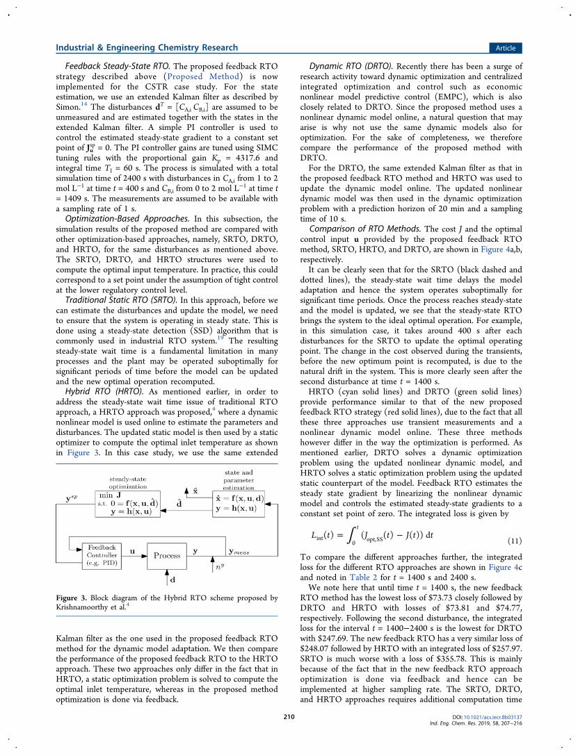
address the steady-state wait time issue of traditional RTOapproach, a HRTO approach was proposed,4 where a dynamicnonlinear model is used online to estimate the parameters anddisturbances. The updated static model is then used by a staticoptimizer to compute the optimal inlet temperature as shownin Figure 3. In this case study, we use the same extended
Kalman filter as the one used in the proposed feedback RTOmethod for the dynamic model adaptation. We then comparethe performance of the proposed feedback RTO to the HRTOapproach. These two approaches only differ in the fact that inHRTO, a static optimization problem is solved to compute theoptimal inlet temperature, whereas in the proposed methodoptimization is done via feedback.
Dynamic RTO (DRTO). Recently there has been a surge ofresearch activity toward dynamic optimization and centralizedintegrated optimization and control such as economicnonlinear model predictive control (EMPC), which is alsoclosely related to DRTO. Since the proposed method uses anonlinear dynamic model online, a natural question that mayarise is why not use the same dynamic models also foroptimization. For the sake of completeness, we thereforecompare the performance of the proposed method withDRTO.For the DRTO, the same extended Kalman filter as that in
the proposed feedback RTO method and HRTO was used toupdate the dynamic model online. The updated nonlineardynamic model was then used in the dynamic optimizationproblem with a prediction horizon of 20 min and a samplingtime of 10 s.
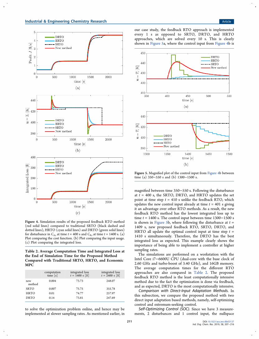
Comparison of RTO Methods. The cost J and the optimalcontrol input u provided by the proposed feedback RTOmethod, SRTO, HRTO, and DRTO, are shown in Figure 4a,b,respectively.It can be clearly seen that for the SRTO (black dashed and
dotted lines), the steady-state wait time delays the modeladaptation and hence the system operates suboptimally forsignificant time periods. Once the process reaches steady-stateand the model is updated, we see that the steady-state RTObrings the system to the ideal optimal operation. For example,in this simulation case, it takes around 400 s after eachdisturbances for the SRTO to update the optimal operatingpoint. The change in the cost observed during the transients,before the new optimum point is recomputed, is due to thenatural drift in the system. This is more clearly seen after thesecond disturbance at time t = 1400 s.HRTO (cyan solid lines) and DRTO (green solid lines)
provide performance similar to that of the new proposedfeedback RTO strategy (red solid lines), due to the fact that allthese three approaches use transient measurements and anonlinear dynamic model online. These three methodshowever differ in the way the optimization is performed. Asmentioned earlier, DRTO solves a dynamic optimizationproblem using the updated nonlinear dynamic model, andHRTO solves a static optimization problem using the updatedstatic counterpart of the model. Feedback RTO estimates thesteady state gradient by linearizing the nonlinear dynamicmodel and controls the estimated steady-state gradients to aconstant set point of zero. The integrated loss is given by
∫= −L t J t J t t( ) ( ( ) ( )) dt
int0 opt,SS (11)
To compare the different approaches further, the integratedloss for the different RTO approaches are shown in Figure 4cand noted in Table 2 for t = 1400 s and 2400 s.We note here that until time t = 1400 s, the new feedback
RTO method has the lowest loss of $73.73 closely followed byDRTO and HRTO with losses of $73.81 and $74.77,respectively. Following the second disturbance, the integratedloss for the interval t = 1400−2400 s is the lowest for DRTOwith $247.69. The new feedback RTO has a very similar loss of$248.07 followed by HRTO with an integrated loss of $257.97.SRTO is much worse with a loss of $355.78. This is mainlybecause of the fact that in the new feedback RTO approachoptimization is done via feedback and hence can beimplemented at higher sampling rate. The SRTO, DRTO,and HRTO approaches requires additional computation time
Figure 3. Block diagram of the Hybrid RTO scheme proposed byKrishnamoorthy et al.4
Industrial & Engineering Chemistry Research Article
to solve the optimization problem online, and hence may beimplemented at slower sampling rates. As mentioned earlier, in
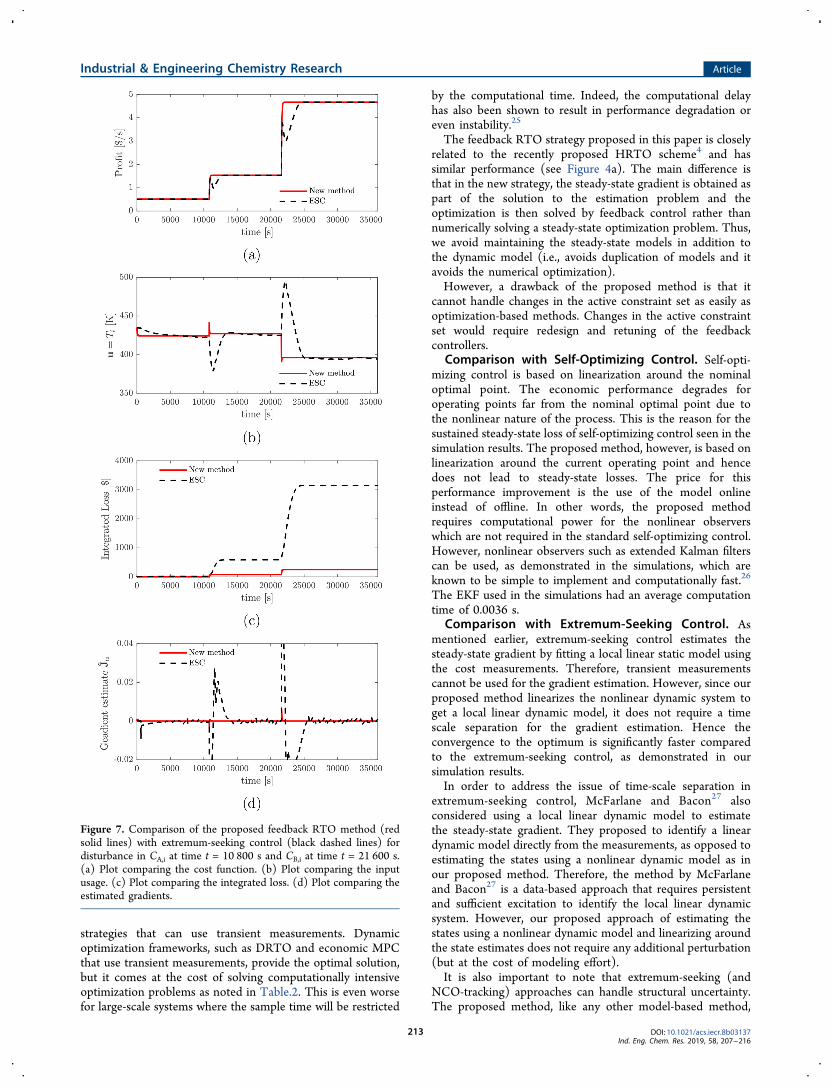
our case study, the feedback RTO approach is implementedevery 1 s as opposed to SRTO, DRTO, and HRTOapproaches, which are solved every 10 s. This is clearlyshown in Figure 5a, where the control input from Figure 4b is
magnified between time 350−550 s. Following the disturbanceat t = 400 s, the SRTO, DRTO, and HRTO updates the setpoint at time step t = 410 s unlike the feedback RTO, whichupdates the new control input already at time t = 401 s givingit an advantage over other RTO methods. As a result, the newfeedback RTO method has the lowest integrated loss up totime t = 1400 s. The control input between time 1300−1500 sis shown in Figure 5b, where following the disturbance at t =1409 s, new proposed feedback RTO, SRTO, DRTO, andHRTO all update the optimal control input at time step t =1410 s simultaneously. Therefore, the DRTO has the bestintegrated loss as expected. This example clearly shows theimportance of being able to implement a controller at highersampling rates.The simulations are performed on a workstation with the
Intel Core i7−6600U CPU (dual-core with the base clock of2.60 GHz and turbo-boost of 3.40 GHz), and 16GB memory.The average computation times for the different RTOapproaches are also compared in Table 2. The proposedfeedback RTO method is the least computationally intensivemethod due to the fact the optimization is done via feedback,and as expected, DRTO is the most computationally intensive.
Comparison with Direct-Input Adaptation Methods. Inthis subsection, we compare the proposed method with twodirect input adaptation based methods, namely, self-optimizingcontrol and extremum-seeking control.
Self-Optimizing Control (SOC). Since we have 3 measure-ments, 2 disturbances and 1 control input, the nullspace
Figure 4. Simulation results of the proposed feedback RTO method(red solid lines) compared to traditional SRTO (black dashed anddotted lines), HRTO (cyan solid lines) and DRTO (green solid lines)for disturbance in CA,i at time t = 400 s and CB,i at time t = 1400 s. (a)Plot comparing the cost function. (b) Plot comparing the input usage.(c) Plot comparing the integrated loss.
Table 2. Average Computation Time and Integrated Loss atthe End of Simulation Time for the Proposed MethodCompared with Traditional SRTO, HRTO, and EconomicMPC
method can be used to identify the self-optimizing variable. Forthe case-study considered here, the optimal selection matrixcomputed using nullspace method (around the nominaloptimal point when dT = [CA,i CB,i]=[1.0 0.0]) is given by H= [−0.76880 63940 0046], see Alstad Ch.4.16. The resultingself-optimizing variable c = −0.7688CA + 0.6394CB + 0.0046Tis controlled to a constant set point of cs = 1.9012. The PIcontroller tunings used in the self-optimizing control structurewere tuned using SIMC rules with proportional gain Kp =188.65 and integral time TI = 75 s.The simulations were performed with the same disturbances
as in the previous case. The objective function for the twomethods are shown in Figure 6a, and the corresponding
control input usage is shown in Figure 6b. When compared toself-optimizing control, we can see that there is an optimalitygap when the disturbances occur. This is because self-optimizing control is based on linearization around thenominal optimal point, as opposed to linearization aroundthe current operating point in the proposed feedback RTOapproach. Because of the nonlinear nature of the processes, theeconomic performance degrades for operating points far fromthe nominal optimal point, hence leading to steady-state losses.Extremum Seeking Control (ESC). The concept of
estimating and driving the steady-state gradient to zero inthe proposed feedback RTO strategy is also used in data-drivenmethods such as extremum-seeking control and NCO-tracking.However, the methods are fundamentally different andcomplementary rather than competing.
For the sake of brevity, we restrict our comparison toextremum-seeking control. We consider the least-squares basedextremum-seeking control proposed by Hunnekens et al.20
because it has been shown to provide better performance thanclassical extremum-seeking control.20,21 The least-squaresbased extremum-seeking controller also estimates the gradientrather than just the sign of the gradient.22 The least-squaresbased extremum-seeking controller estimates the steady-stategradient using the measured cost and input data with themoving window of fixed length in the past. The gradientestimated by the least-square method is then driven to zerousing a simple integral action. The integral gain was chosen tobe KESC = 2.Due to the slow convergence of the extremum-seeking
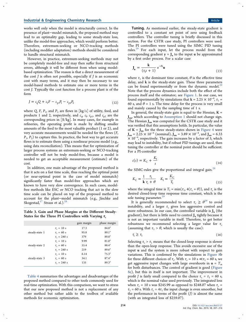
controller, the process with simulated with a total simulationtime of 600 min with disturbances in CA,i from 1 to 2 mol L−1
at time t = 10 800 s and CB,i from 0 to 2 mol L−1 at time t =21 600 s. The results using extremum-seeking control arecompared with that the of the proposed method in Figure 7a.It can be seen that the extremum-seeking controller reachesthe optimal point, however, the convergence to the optimumpoint is very slow compared to the proposed method. Theproposed method has a fast reaction to the disturbances andhence reaches the optimum significantly faster than theextremum-seeking controller. The integrated loss comparedto the ideal steady-state optimum (eq 11) shown in Figure 7creflects this.It should be added this is a simulation example because
strictly speaking it may not be possible to directly measure aneconomic cost J with several terms. The simple cost in eq 10may be computed by measuring individually the compositionCB and the inlet temperature Ti, but more generally for processsystems, direct measurement of all the terms and adding themtogether is not accurate. This is discussed further in theDiscussion.
Other Multivariable Case Studies. In addition to theCSTR case study, the new proposed feedback RTO methodhas been successfully applied to a 3-bed ammonia reactor casestudy by Bonnowitz et al.23 and to an oil and gas productionoptimization problem by Krishnamoorthy et al.24 In all thesecase studies, the new feedback RTO method was comparedwith other optimization methods and was shown to provideconsistent results as in the CSTR case study shown in thispaper. Both these cases studies are multivariable processes,where the steady-state gradients must be estimated andcontrolled to zero.For example, let us consider the ammonia reactor process
studied by Bonnowitz et al.,23 which consists of 3 ammoniareactor beds. The optimization problem is concerned withcomputing the three optimal feeds in order to maximize thereaction extent. The proposed method was applied to thissystem, where the steady-state gradients of the cost withrespect to the three inputs were estimated using eq 7. Thereader is referred to Bonnowitz et al.23 for more detailedinformation about the process and the simulation results,which shows that the proposed method works also for multi-input processes that are coupled together.
■ DISCUSSIONComparison with Optimization-Based Approaches.
With the traditional steady-state RTO approach, it was seenclearly that the steady-state wait time resulted in suboptimaloperation, clearly motivating the need for alternative RTO
Figure 6. Simulation results of the proposed feedback RTO method(red solid lines) compared to self-optimizing control (blue solid lines)for disturbance in CA,i at time t = 400 s and CB,i at time t = 1400 s. (a)Plot comparing the cost function. (b) Plot comparing the input usage.
Industrial & Engineering Chemistry Research Article
strategies that can use transient measurements. Dynamicoptimization frameworks, such as DRTO and economic MPCthat use transient measurements, provide the optimal solution,but it comes at the cost of solving computationally intensiveoptimization problems as noted in Table.2. This is even worsefor large-scale systems where the sample time will be restricted
by the computational time. Indeed, the computational delayhas also been shown to result in performance degradation oreven instability.25
The feedback RTO strategy proposed in this paper is closelyrelated to the recently proposed HRTO scheme4 and hassimilar performance (see Figure 4a). The main difference isthat in the new strategy, the steady-state gradient is obtained aspart of the solution to the estimation problem and theoptimization is then solved by feedback control rather thannumerically solving a steady-state optimization problem. Thus,we avoid maintaining the steady-state models in addition tothe dynamic model (i.e., avoids duplication of models and itavoids the numerical optimization).However, a drawback of the proposed method is that it
cannot handle changes in the active constraint set as easily asoptimization-based methods. Changes in the active constraintset would require redesign and retuning of the feedbackcontrollers.
Comparison with Self-Optimizing Control. Self-opti-mizing control is based on linearization around the nominaloptimal point. The economic performance degrades foroperating points far from the nominal optimal point due tothe nonlinear nature of the process. This is the reason for thesustained steady-state loss of self-optimizing control seen in thesimulation results. The proposed method, however, is based onlinearization around the current operating point and hencedoes not lead to steady-state losses. The price for thisperformance improvement is the use of the model onlineinstead of offline. In other words, the proposed methodrequires computational power for the nonlinear observerswhich are not required in the standard self-optimizing control.However, nonlinear observers such as extended Kalman filterscan be used, as demonstrated in the simulations, which areknown to be simple to implement and computationally fast.26
The EKF used in the simulations had an average computationtime of 0.0036 s.
Comparison with Extremum-Seeking Control. Asmentioned earlier, extremum-seeking control estimates thesteady-state gradient by fitting a local linear static model usingthe cost measurements. Therefore, transient measurementscannot be used for the gradient estimation. However, since ourproposed method linearizes the nonlinear dynamic system toget a local linear dynamic model, it does not require a timescale separation for the gradient estimation. Hence theconvergence to the optimum is significantly faster comparedto the extremum-seeking control, as demonstrated in oursimulation results.In order to address the issue of time-scale separation in
extremum-seeking control, McFarlane and Bacon27 alsoconsidered using a local linear dynamic model to estimatethe steady-state gradient. They proposed to identify a lineardynamic model directly from the measurements, as opposed toestimating the states using a nonlinear dynamic model as inour proposed method. Therefore, the method by McFarlaneand Bacon27 is a data-based approach that requires persistentand sufficient excitation to identify the local linear dynamicsystem. However, our proposed approach of estimating thestates using a nonlinear dynamic model and linearizing aroundthe state estimates does not require any additional perturbation(but at the cost of modeling effort).It is also important to note that extremum-seeking (and
NCO-tracking) approaches can handle structural uncertainty.The proposed method, like any other model-based method,
Figure 7. Comparison of the proposed feedback RTO method (redsolid lines) with extremum-seeking control (black dashed lines) fordisturbance in CA,i at time t = 10 800 s and CB,i at time t = 21 600 s.(a) Plot comparing the cost function. (b) Plot comparing the inputusage. (c) Plot comparing the integrated loss. (d) Plot comparing theestimated gradients.
Industrial & Engineering Chemistry Research Article
works well only when the model is structurally correct. In thepresence of plant−model mismatch, the proposed method maylead to an optimality gap, leading to some steady-state loss,unlike the model-free approaches, which would perform better.Therefore, extremum-seeking or NCO-tracking methods(including modifier adaptation) methods should be consideredto handle structural mismatch.However, in practice, extremum-seeking methods may not
be completely model-free and may then suffer from structuralerrors, although it will be different from when using model-based optimization. The reason is that a direct measurement ofthe cost J is often not possible, especially if J is an economiccost with many terms, and it may then be necessary to usemodel-based methods to estimate one or more terms in thecost J. Typically the cost function for a process plant is of theform
= + − −J c Q c F c P c Pq f p1 1 p2 2 (12)
where Q, F, P1, and P2 are flows in [kg/s] of utility, feed, andproducts 1 and 2, respectively, and cq, cf, cp1, and cp2 are thecorresponding prices in [$/kg]. In many cases, for example inrefineries, the operating profit is made by shifting smalleramounts of the feed to the most valuable product (1 or 2), andvery accurate measurements would be needed for the flows (F,P1, P2) to capture this. In practice, the best way to get accurateflows is to estimate them using a nonlinear process model (e.g.,using data reconciliation). This means that for optimization oflarger process systems an extremum-seeking or NCO-trackingcontroller will not be truly model-free, because a model isneeded to get an acceptable measurement (estimate) of thecost.In addition, one main advantage of the proposed method is
that it acts on a fast time scale, thus reaching the optimal point(or near-optimal point in the case of model mismatch)significantly faster than model-free approaches which areknown to have very slow convergence. In such cases, model-free methods like ESC or NCO tracking that act in the slowtime scale can be placed on top of the proposed method toaccount for the plant−model mismatch (e.g., Jaschke andSkogestad,17 Straus et al.).28
Table 4 summarizes the advantages and disadvantages of theproposed method compared to other tools commonly used forreal-time optimization. With this comparison, we want to stressthat our new proposed method is not a replacement of anyother method but rather adds to the toolbox of availablemethods for economic optimization.
Tuning. As mentioned earlier, the steady-state gradient iscontrolled to a constant set point of zero using feedbackcontrollers. The controller tuning is briefly discussed in thissection. For the CSTR case study, PI controllers were used.The PI controllers were tuned using the SIMC PID tuningrules.29 For each input, let the process model from thecorresponding gradient y = Ju to the input u be approximatedby a first order process. For a scalar case
τ=
+θ−
sJ
ku
( 1)e s
u1 (13)
where τ1 is the dominant time constant, θ is the effective timedelay, and k is the steady-state gain. These three parameterscan be found experimentally or from the dynamic model.29
Note that the process dynamics include both the effect of theprocess itself and the estimator; see Figure 1. In our case, wefound experimentally by simulations that k = 2.25 × 10⁻⁴, τ1 =60 s, and θ = 1 s. The time delay for the process is very smalland mainly caused by the sampling time of 1 s.In general, the steady-state gain is equal to the Hessian, K =
Juu, which according to Assumption 1 should not change sign.The Hessian Juu was computed for the CSTR case study and itwas verified that this assumptions holds. In particular, the valueof K = Juu for the three steady-states shown in Figure 4 wereJuu = 2.25 × 10⁻⁴ (nominal), Juu = 3.89 × 10⁻⁴, and Juu = 6.33× 10⁻⁴, respectively. The gain increases by a factor of 3, whichmay lead to instability, but if robust PID tunings are used, thentuning the controller at the nominal point should be sufficient.For a PI-controller
= +c s KKs
( ) CI
(14)
the SIMC-rules give the proportional and integral gain.29
ττ θ
=+
=K KKTk
1C
1
cI
C
I (15)
where the integral time is TI = min(τ1, 4(τc + θ)), and τc is thedesired closed-loop time response time constant, which is thesole tuning parameter.29
It is generally recommended to select τc ≥ θ29 to avoidinstability, and a larger τc gives less aggressive control andmore robustness. In our case, the controlled variable is Ju (thegradient), but there is little need to control Ju tightly because itis not an important variable in itself. Therefore, to get betterrobustness we recommend selecting a larger value for τc(assuming that τ1 > θ, which is usually the case):
τ τ≥c 1 (16)
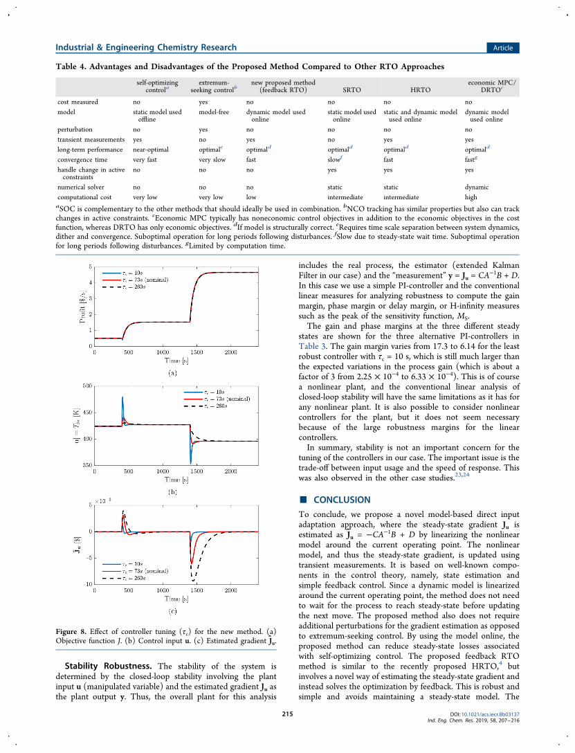
Selecting τc > τ1 means that the closed-loop response is slowerthan the open-loop response. This avoids excessive use of theinput u and the system is more robust with respect to gainvariations. This is confirmed by the simulations in Figure 8bfor three different choices of τc. With τc = 10 s ≪τ1 = 60 s, weget aggressive input changes with large overshoots in u = Tinfor both disturbances. The control of gradient is good (Figure8c), but this in itself is not important. The improvement inprofit J is fairly small compared to the choice τc = τ1 = 60 s,which is the nominal value used previously. The integrated losswhen τc = 10 s was $245.99 as opposed to $248.07 when τc =τ1 = 60 s. With τc = 4τ1 the input change is even smoother, butthe performance in terms of the profit (J) is almost the same(with an integrated loss of $259.07).
Table 3. Gain and Phase Margins at the Different Steady-States for the Three PI Controllers with Varying τc
gain margin phase margin
steady-state 1τc = 10 s 17.3 84.8°τc = 60 s 95.8 89.1°τc = 240 s 379 89.8°
steady-state 2τc = 10 s 9.99 81.0°τc = 60 s 55.4 88.4°τc = 240 s 219 89.6°
steady-state 3τc = 10 s 6.14 75.3°τc = 60 s 34.1 87.4°τc = 240 s 135 89.3°
Industrial & Engineering Chemistry Research Article
Stability Robustness. The stability of the system isdetermined by the closed-loop stability involving the plantinput u (manipulated variable) and the estimated gradient Ju asthe plant output y. Thus, the overall plant for this analysis
includes the real process, the estimator (extended KalmanFilter in our case) and the “measurement” y = Ju = CA−1B + D.In this case we use a simple PI-controller and the conventionallinear measures for analyzing robustness to compute the gainmargin, phase margin or delay margin, or H-infinity measuressuch as the peak of the sensitivity function, MS.The gain and phase margins at the three different steady
states are shown for the three alternative PI-controllers inTable 3. The gain margin varies from 17.3 to 6.14 for the leastrobust controller with τc = 10 s, which is still much larger thanthe expected variations in the process gain (which is about afactor of 3 from 2.25 × 10⁻⁴ to 6.33 × 10⁻⁴). This is of coursea nonlinear plant, and the conventional linear analysis ofclosed-loop stability will have the same limitations as it has forany nonlinear plant. It is also possible to consider nonlinearcontrollers for the plant, but it does not seem necessarybecause of the large robustness margins for the linearcontrollers.In summary, stability is not an important concern for the
tuning of the controllers in our case. The important issue is thetrade-off between input usage and the speed of response. Thiswas also observed in the other case studies.23,24
■ CONCLUSION
To conclude, we propose a novel model-based direct inputadaptation approach, where the steady-state gradient Ju isestimated as J u = −CA−1B + D by linearizing the nonlinearmodel around the current operating point. The nonlinearmodel, and thus the steady-state gradient, is updated usingtransient measurements. It is based on well-known compo-nents in the control theory, namely, state estimation andsimple feedback control. Since a dynamic model is linearizedaround the current operating point, the method does not needto wait for the process to reach steady-state before updatingthe next move. The proposed method also does not requireadditional perturbations for the gradient estimation as opposedto extremum-seeking control. By using the model online, theproposed method can reduce steady-state losses associatedwith self-optimizing control. The proposed feedback RTOmethod is similar to the recently proposed HRTO,4 butinvolves a novel way of estimating the steady-state gradient andinstead solves the optimization by feedback. This is robust andsimple and avoids maintaining a steady-state model. The
Table 4. Advantages and Disadvantages of the Proposed Method Compared to Other RTO Approaches
self-optimizingcontrola
extremum-seeking controlb
new proposed method(feedback RTO) SRTO HRTO
economic MPC/DRTOc
cost measured no yes no no no nomodel static model used
offlinemodel-free dynamic model used
onlinestatic model usedonline
static and dynamic modelused online
dynamic modelused online
perturbation no yes no no no notransient measurements yes no yes no yes yeslong-term performance near-optimal optimale optimald optimald optimald optimald
convergence time very fast very slow fast slowf fast fastg
handle change in activeconstraints
no no no yes yes yes
numerical solver no no no static static dynamiccomputational cost very low very low low intermediate intermediate highaSOC is complementary to the other methods that should ideally be used in combination. bNCO tracking has similar properties but also can trackchanges in active constraints. cEconomic MPC typically has noneconomic control objectives in addition to the economic objectives in the costfunction, whereas DRTO has only economic objectives. dIf model is structurally correct. eRequires time scale separation between system dynamics,dither and convergence. Suboptimal operation for long periods following disturbances. fSlow due to steady-state wait time. Suboptimal operationfor long periods following disturbances. gLimited by computation time.
Figure 8. Effect of controller tuning (τc) for the new method. (a)Objective function J. (b) Control input u. (c) Estimated gradient Ju.
Industrial & Engineering Chemistry Research Article
proposed method is tested in simulations, and compared tocommonly used optimization-based approaches and direct-input adaptation-based approaches. The simulation resultsshow that the proposed method is accurate, fast and easy toimplement. The proposed method thus adds on to the existingtoolbox of approaches for real-time optimization, and can beuseful for certain cases.
ORCIDDinesh Krishnamoorthy: 0000-0002-9947-8690NotesThe authors declare no competing financial interest.
■ ACKNOWLEDGMENTS
The authors gratefully acknowledge the financial support fromSFI SUBPRO, which is financed by the Research Council ofNorway, major industry partners and NTNU.
■ REFERENCES(1) Darby, M. L.; Nikolaou, M.; Jones, J.; Nicholson, D. RTO: Anoverview and assessment of current practice. J. Process Control 2011,21, 874−884.(2) Chachuat, B.; Srinivasan, B.; Bonvin, D. Adaptation strategies forreal-time optimization. Comput. Chem. Eng. 2009, 33, 1557−1567.(3) Francois, G.; Srinivasan, B.; Bonvin, D. Comparison of siximplicit real-time optimization schemes. Journal Europeen des SystemesAutomatises 2012, 46, 291−305.(4) Krishnamoorthy, D.; Foss, B.; Skogestad, S. Steady-state Realtime optimization using transient measurements. Comput. Chem. Eng.2018, 115, 34−45.(5) Skogestad, S. Plantwide control: The search for the self-optimizing control structure. J. Process Control 2000, 10, 487−507.(6) Jaschke, J.; Cao, Y.; Kariwala, V. Self-optimizing control−Asurvey. Annual Reviews in Control 2017, 43, 199−223.(7) Krstic, M.; Wang, H.-H. Stability of extremum seeking feedbackfor general nonlinear dynamic systems. Automatica 2000, 36, 595−601.(8) Ariyur, K. B.; Krstic, M. Real-time optimization by extremum-seeking control; John Wiley & Sons, 2003.(9) Francois, G.; Srinivasan, B.; Bonvin, D. Use of measurements forenforcing the necessary conditions of optimality in the presence ofconstraints and uncertainty. J. Process Control 2005, 15, 701−712.(10) Kumar, V.; Kaistha, N. Hill-Climbing for Plantwide Control toEconomic Optimum. Ind. Eng. Chem. Res. 2014, 53, 16465−16475.(11) Tan, Y.; Moase, W.; Manzie, C.; Nesic, D.; Mareels, I.Extremum seeking from 1922 to 2010. Proceedings of 2010 29thChinese Control Conference (CCC); Beihang University Press, 2010; pp14−26.(12) Trollberg, O.; Jacobsen, E. W. Greedy Extremum SeekingControl with Applications to Biochemical Processes. IFAC-PapersOn-Line (DYCOPS-CAB) 2016, 49, 109−114.(13) Srinivasan, B.; Francois, G.; Bonvin, D. Comparison of gradientestimation methods for real-time optimization. Comput.-Aided Chem.Eng. 2011, 29, 607−611.(14) Simon, D. Optimal State Estimation, Kalman, H-infinity andNonlinear Approches; Wiley-Interscience: Hoboken, NJ, 2006.(15) Economou, C. G.; Morari, M.; Palsson, B. O. Internal modelcontrol: Extension to nonlinear system. Ind. Eng. Chem. Process Des.Dev. 1986, 25, 403−411.(16) Alstad, V. Studies on Selection of Controlled Variables. Ph.D.Thesis. Norwegian University of Science and Technology, 2005.
(17) Jaschke, J.; Skogestad, S. NCO tracking and self-optimizingcontrol in the context of real-time optimization. J. Process Control2011, 21, 1407−1416.(18) Ye, L.; Cao, Y.; Li, Y.; Song, Z. Approximating NecessaryConditions of Optimality as Controlled Variables. Ind. Eng. Chem. Res.2013, 52, 798−808.(19) Camara, M. M.; Quelhas, A. D.; Pinto, J. C. PerformanceEvaluation of Real Industrial RTO Systems. Processes 2016, 4, 44.(20) Hunnekens, B.; Haring, M.; van de Wouw, N.; Nijmeijer, H. Adither-free extremum-seeking control approach using 1st-order least-squares fits for gradient estimation. IEEE 53rd Annual Conference onDecision and Control (CDC) 2014, 2679−2684.(21) Chioua, M.; Srinivasan, B.; Guay, M.; Perrier, M. PerformanceImprovement of Extremum Seeking Control using Recursive LeastSquare Estimation with Forgetting Factor. IFAC-PapersOnLine(DYCOPS-CAB) 2016, 49, 424−429.(22) Chichka, D. F.; Speyer, J. L.; Park, C. Peak-seeking control withapplication to formation flight. Proceedings of the 38th IEEE Conferenceon Decision and Control 1999, 2463−2470.(23) Bonnowitz, H.; Straus, J.; Krishnamoorthy, D.; Jahanshahi, E.;Skogestad, S. Control of the Steady-State Gradient of an AmmoniaReactor using Transient Measurements. Comput.-Aided Chem. Eng.2018, 43, 1111−1116.(24) Krishnamoorthy, D.; Jahanshahi, E.; Skogestad, S. Gas-liftOptimization by Controlling Marginal Gas-Oil Ratio using TransientMeasurements. IFAC-PapersOnLine 2018, 51, 19−24.(25) Findeisen, R.; Allgower, F. Computational delay in nonlinearmodel predictive control. IFAC Proceedings Volumes 2004, 37, 427−432.(26) Sun, X.; Jin, L.; Xiong, M. Extended Kalman filter forestimation of parameters in nonlinear state-space models ofbiochemical networks. PLoS One 2008, 3, No. e3758.(27) McFarlane, R.; Bacon, D. Empirical strategies for open-loop on-line optimization. Can. J. Chem. Eng. 1989, 67, 665−677.(28) Straus, J.; Krishnamoorthy, D.; Skogestad, S. Combining self-optimizing control and extremum seeking control - Applied toammonia reactor case study. AIChE Annual Meeting 2017;Minneapolis, MN, 2017.(29) Skogestad, S. Simple analytic rules for model reduction andPID controller tuning. J. Process Control 2003, 13, 291−309.
Industrial & Engineering Chemistry Research Article