Feedforward Frequency Estimation for PSK: a Tbtorial Review

MICHELE MORELLI, UMBERTO MENGAL1 Dipartimento di Ingegneria della Informazione, Universitl di Pisa

Via Diotisalvi 2,56100 Pisa - Italy morelli, mengali @iet.unipi.it

Abstract. This paper considers feedforward carrier frequency estimation methods in burst-mode digital transmission, with tutorial objectives foremost. Assuming PSK modulation, two scenarios are envisaged in which frequency estimates are derived either from a preamble appended to the data block, or directly from the modulated signal. Several estimation algorithms are considered with different and somewhat contrasting characteristics. The characteristics we focus on are: estimation accuracy, estimation range, minimum operating signal-to-noise ratio (threshold), and implementation complexity. They provide a frame- work within which current estimation methods can be evaluated. The paper reviews and compares some prominent algorithms proposed in literature, trying to single out the best ones for a given application.

1. INTRODUCTION

Burst-mode transmission of digital data is employed in many applications such as satellite time-division multi- ple-access (TDMA) techniques and terrestrial mobile cel- lular radio. In conventional systems a preamble of known symbols is placed somewhere in each burst for carrier and clock recovery purposes. The use of the preamble allows data-aided (DA) operation and results in superior perfor- mance in comparison with non-data-aided (NDA) meth- ods. Even so, synchronization may prove difficult, espe- cially with coded modulations. For example, with QPSK signaling and rate 1/2, constraint length 7, convolutional coding, the signal-to-noise ratio E,/N,, needed to achieve a bit error rate of 10-6 is only 5 dB. Since it is desirable that the transmission system continues to operate even at higher error rates, a minimum of 2-3 dB is often set as a design target. Clearly, very efficient synchronization algorithms are needed in these conditions.

Ideally, preambles should be as short as possible for they reduce the transmission rate. For example, current trends in satellite transmission for LAN interconnection indicate that an overhead of 10% is quite feasible [l]. Clearly, the next step is to get rid of preambles altogeth- er and estimate the synchronization parameters in an NDA fashion [2]. This route raises the following ques- tion. Lack of data information is expected to degrade synchronization accuracy for afixed estimation time. On the other hand, the estimation time does not need to be as short as when a preamble is used. In fact the whole

data burst is available, not just a segment of it. Then, one wonders whether the extended estimation time will compensate for the NDA operation. The answer is not obvious and depends on the specific algorithms being used. For example, in [3] it is shown that carrier phase can be efficiently estimated without any preamble.

In this paper we concentrate on carrier frequency estimation with PSK signaling. Our aim is to compare various feedforward estimation algorithms, either DA or NDA, that have been proposed in literature. In doing so we describe their features in terms of four performance indexes:

i) estimation accuracy; ii) estimation range; iii) threshold (the critical signal-to-noise ratio below

which large estimation errors begin to occur); iv) implementation complexity.

It is worth noting that these indexes may be in contrast with each other. For example, achieving a low threshold implies a high complexity. Likewise, good estimation accuracy is often met at the price of a narrow estimation range. So, a trade off is called for between conflicting requirements and a judicious choice between various options can only be made by carefully specifying the actual operating conditions.

The remainder of the paper is organized as follows. The next section concentrates on the signal model and describes the statistics of the sequence [ z ( k ) ] as obtained

Vol. 9. No. 2 March - April I998 I03

by eliminating the modulation from the samples at the matched filter output. Section 3 describes an algorithm derived from maximum likelihood criteria. Simpler methods are indicated in section 4. Other algorithms, based on correlation calculations, are reported in section 5. Computational complexity considerations are addres- sed in section 6 . Finally, some conclusions are offered in section 7.

2. SIGNAL MODEL

In this study we make the following major assump- tions. The modulation is PSK and the channel noise is additive, white and Gaussian, with two-sided power spectral density N0/2. The channel filtering is equally apportioned between transmitter and receiver and the overall channel response is Nyquist in the absence offre- quency errors. Clock recovery is ideal. Indeed, excellent timing information can normally be derived even with frequency errors on the order of 10-20% of the symbol rate. In these conditions it is readily shown that the sam- ples from the matched filter are given by

x ( k ) = Ck ej(2nfdkT;+@ + n(k) (1)

where ( c k ) are data symbols from the PSK alphabet ( e‘ZdM; rn = 0, 1,. . ., M - 1 ), fd is the carrier frequency offset we want to estimate, 8 represents the carrier phase, T is the symbol period, [ n ( k ) ] are zero-mean Gaussian random variables with independent real and imaginary components, each of variance (Es/N0)-I/2, and E, is the signal energy per symbol. The phase 8 is uniformly distributed over [0,27r).

It should be stressed that eq. (1) holds true only with rather limited values of fd (on the order of few percents of the symbol rate). In fact the right hand side does not reflect the mismatching between the’ incoming signal and the receive filter due to frequency emors. Actually, an exact expression for x( r ) is

i t k

where h(t) is the convolution

tude ( I h(0) I c 1). For heuristic reasons in the sequel we adopt the model ( I ) but the effects of intersymbol inter- ference will be pointed out in due time.

It is clear from (1) that the samples x( r ) depend on the modulation. As most frequency estimation algo- rithms are tailored for unmodulated carriers, the data symbols must be wiped out in some way. Two different approaches can be followed to do so, depending on whether the trasmitted symbols ( c k } are known or not. The first instance corresponds to DA algorithms and is handled by multiplying both sides of (1) by c; (the superscript “star” means complex conjugate) to yield

z ( k ) = x(k ) c; DA operation ( 5 )

from which, bearing in mind that ck has unit amplitude, we get

where n’(k) 4 n ( k ) c; is a noise sequence statistically equivalent to [n(k) ] . Eq. (6) indicates that z ( k ) is a sine wave embedded in noise. In the next sections we dis- cuss how to estimate its frequency from the observation of [z(k)l.

In the absence of a preamble the modulation can be removed by feeding x ( k ) into some ad hoc non linearity [ 3 ] . The simplest and only type of non linearity we con- sider in this study consists of raising x ( k ) to the M- power (M is the number of modulation levels) and scal- ing the result to unit amplitude. Formally, the output of the non linearity is related to the input x ( k ) by

It is readily checked that (7) may also be written as

where

( 3 )

and g(t) is the shape of the modulation pulses. Bear in mind that we have assumed a Nyquist h(r) forfJ = 0, i.e.,

Comparing ( 1 ) and (2) we see that they coincide only for very small frequency offsets. Otherwise, they are different because of the presence of intersymbol inter- ference in (2) and a reduction in the useful signal ampli-

Thus, we have again a sine wave but, in comparison to (6). its frequency is M times larger and the channel noise affects z (k ) only through a non-Gaussian phase disturbance qk.

It is interesting to compare DA and NDA operations at high SNR. To this purpose let us rewrite ( 6 ) in the form

or, equivalently,

104

Clearly, the amplitude of n"(k) becomes smaller and smaller relative to unity as E,/N, increases. Then, (12) tends to (8) with M = 1. In other words, at high SNR the model (8) is valid for both DA and NDA operations provided that we set M = 1 when dealing with DA.

3. RIFE AND BOORSTYN ALGORITHM

Having established a statistical model for the observ- ables [ ~ ( k ) ] , we now concentrate on frequency estima- tion algorithms. A powerful method has been indicated by Rife and Boorstyn (R&B) in [4]. Let us see how it works when the data are available (DA operation). Taking ( 6 ) as an exact model ( I ) , Rife and Boorstyn have shown that the maximum likelihood (ML) estimate of fd is the location where the amplitude of

achieves a maximum, Lo being the observation length in symbol intervals. Formally, the R&B estimator reads

From ( 6 ) it is readily checked that fd is independent of the carrier phase 8. It is also evident that Zcf) is a periodic function of period 1/T. This implies that the estimates provided by (14) are ambiguous by multiples of the symbol rate or, in other words, that the estimation range is &1/(27).

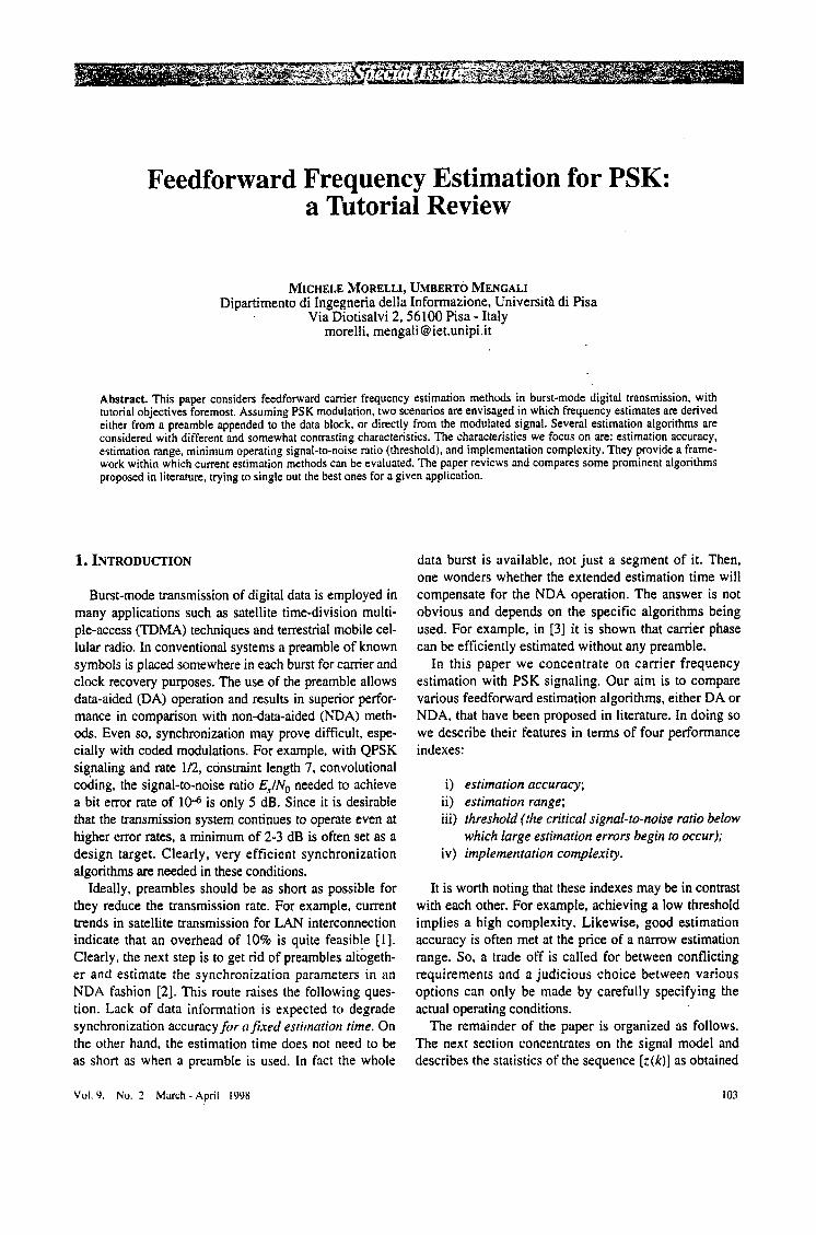
One difficulty with locating the maximum of Z(f) is apparent from Fig. 1 a) which illustrates a typical realiza- tion of I Zy) I as obtained by simulation with QPSK sig- naling and root-raised-cosine-rolloff (RRCR) pulses with rolloff a = 0.5. The observation length is L,, = 64 and Es/No is 10 dB. Also, the normalized frequency offsetfdl" is chosen equal to 0.1. As there are many local maxima, the largest maximum must be sought in two steps. The first one (coarse search) calculates Zcf, over a discrete set of f-values covering the uncertainty range of fd and determines that f which maximizes I Zy) I. The second step Vine search) interpolates between samples of 1 Zy) I and computes the local maximum nearest to the f-value picked up earlier. Note that, occasionally, I Zy) I will be so distorted by noise that its highest peak will be far from fd. When this happens the R&B algorithm makes large errors (outliers). The SNR below which the outliers start to wxur is referred to as the threshold of the estimator.

Fig. 1 b) illustrates a realization of 120 I as obtained with the same parameters of Fig. 1 a), except that Es/No is now -10 dB. An outlier is clearly evident. Therefore,

( I ) As mentioned in section 2, eq. (6) is only valid with small frequen- cy offsets. Whenf, increases. the receive filter is no longer matched to the incoming pulses and the more complex model (2) must be taken into account.

0.4 U

0.2 -

nn ".Y

-0.50 -0.25 0.0 0.1 0.25 0.50 Normalized Frequency, ff

1.2 1

1 .o - 5 0.8

.z - 0.6 0.4

N -

C LL.

0.2

n o

b) -0.50 -0.25 0.0 0.1 0.25 0.50

Normalized Frequency, ff

Fig. 1 a) A typical realization of 1 Zy) 1 for EJN, = 10 dB; b) 120 I for EJN, = -10 dB

the coarse search will provide an estimate of fd of about 0.3/T instead of fd = O.I/T. Since large errors have dis- abling effects on the receiver performance, frequency estimators must operate above threshold.

In practice the coarse search can be efficiently per- formed using Fast Fourier Transform (FlT) techniques [ 4 ] , as is now explained. First, z ( k ) is zero-padded up to some length &K, yielding the sequence

where K is a parameter called pruning factor. Second, the FFT of [ ~ ' ( k ) ] is computed at the points

to produce the set [Z(f,)]. Finally, the largest I Z(fJ I is sought and this gives the coarse frequency estimate.

The choice of the pruning factor considerably affects the estimation performance. Rife and Boorstyn recorn- mend K values in the range from 2 to 8 to keep the threshold low. In these conditions their estimator turns out to be unbiased in the range *1/(27).

Fig. 2 illustrates the accuracy of the R&B algorithm with QPSK modulation and root-raised-cosine-rolloff pulses with 50% roiloff, say RRCR(SO%). The ordi- nates give the estimation error variance normalized to the squared symbol rate. The pruning factor is K = 4

VOI. 9, NO.? Mxch- April 1998 I05

1 P ' O -5 0 5 10 15 20 25 30

Y N a dB Fig. 2 - Accuracy of R&B algorithm with DA operation.

and the observation interval is of 64 symbols. The low- est line represents the modified Cramer-Rao bound (MCRB) [5] which is given by

T 2 xMCRB(f,)=-- 3 1 2 x 2 G E , / N o

We see that the estimation accuracy keeps quite close to the bound up to E,IN, values below 0 dB. If E,INo is decreased further, however, a rapid increase in the error variance is observed. The abscissa at which the slope of the curve starts to change indicates the estimator threshold and is a manifestation of the occurrence of outliers. The mismatching between the incoming signal and the receiv- ing filter deteriorates the performance as& increases.

Next we turn our attention to NDA operation. Recall- ing the comments at the end of the previous section it is clear that the R&B estimator can be used even for NDA operation provided that the sequence [ z (k) ] is computed from (7) rather than (5). Also, bearing in mind that eq. (8) holds for either DA and NDA at high SNR (with M = 1 for DA), it can be shown that NDA operation leads to an estimation ambiguity by multiples of IIMT, not 1/T as happens with DA operation. For example, with 8PSK modulation the estimation range reduces from &SIT to +0.0625/T in passing from DA to NDA.

Fig. 3 shows simulation results for NDA operation. The modulation is still QPSK, the pruning factor is K = 4 and the frequency offset is chosen equal to zero. The modified Cramer-Rao bounds corresponding to the vari- ous observation lengths are indicated. We see that the threshold is a decreasing function of &. Approximately, doubling Lo results in a threshold decrease by 2 dB. This feature of the R&B estimator is of great impor- tance with coded modulation for it makes this estimator

Fig. 3 - Accuracy of R&B algorithm with NDA operation.

suitable for operation at very low SNR (by adequately increasing the observation length). As we shall see, other estimators have a threshold almost independent of 4, and, in consequence, they can only be employed at intermediatehigh SNR.

Fig. 4 illustrates further results with NDA operation. Everything is as in Fig. 3, except that the modul.ation is 8PSK. The curves have still the same shape but, as expected, the threshold is now considerably higher for a given observation length.

10'3

104

1 P l@

I 10-'

10-8

10-0

10-10 0 5 10 15 20 25 30

%"a dB Fig. 4 -Accuracy of R&B algorithm with NDA operation and SPSK.

I06 ETT

4. LEAST-SQUARES-BASED ESTIMATORS

4.1. Tretter Estimator

The R&B estimator has very good performance but, as we shall see later, has a rather high computational com- plexity. Simpler methods are desirable and, in fact, a number of alternatives have been proposed in literature. In this section we describe two schemes derived from least squares estimation criteria. Our goal is to indicate their logical basis and give an idea of their performance. In pursuing this task we shall employ the model (8) which is valid at high SNR for either DA and NDA operation. It should be stressed that adopting this model has only heur- istic purposes for, in effect, the algorithms we shall obtain are useful at any SNR (not necessarily high).

The first algorithm has been proposed by Tretter [6] and is based on the following considerations. From (8) we see that

With this adjustment the Tretter estimator takes its final form

4.2. Kay estimator

Kay [7] has shown that the unwrapping process can be obviated if the sequence (arg [ z ( k ) z* ( k - l)]} is used in place of (arg [ ~ ( k ) ] } . To see how this comes about observe that

Then, from ( I 8) we have where the modulo-2x operation [XI:* means that x is reduced to the interval (-x, x]. Suppose for the moment that the variable M (2xkfdT + 8 + q k ) is within the interval (-9 x] (which may not be true since the ampli- tude of M (2xkfdT + 8 + qk) increases unboundedly with k ) . Then the modulo-2x operation in (18) is imma- terial and the right hand side may be viewed as noisy samples of a straight line with slope M2xfdT. Clearly, estimating the slope of this line amounts to estimating fd, for the two quantities are proportional. Tretter [6] approaches this problem by least squares methods and comes up with the following solution

where [win] are weighting coefficients given by

To reiterate, eq. (19) is valid for either DA and NDA operation. In the former, the parameter M equals unity and z ( k ) is computed from (5); in the latter, M equals the number of points in the signal constellation and z ( k ) is computed from (7).

A drawback with (19) is that the modulo-2x opera- tion cannot be ignored as it produces jumps by 2 x in the trajectory of arg [ z ( k ) ] when M (2xkfdT + 8 + q k ) crosses odd multiples of x. Luckily the jumps can be eliminated by unwrapping the sequence (arg [zik)]}. The unwrapping algorithm produces a new sequence [pun) ( k ) ] which is related to (arg [~(k)]} by

Vol. 9. No. 2 March - April 1998

Comparing with (18) it appears that the useful term in the right hand side in (18) has been turned into a constant, 2xM&T. In consequence, the chance of phase 'umps has been greatly reduced, especially if 2 7 ~ ~ 1 fd r' T is well internal to +n and the SNR is high. Then, paralleling the arguments leading to (19) produces the Kay estimator

where the weights wLm are given by

An essentially identical algorithm has been proposed by Bellini, Molinari and Tartara in [8].

It is a simple matter to show that Tretter and Kay estimators are equivalent. To see why, let us compare (21) with (23). We have

Next, substituting into (26) yields c

On the other hand it is readily checked from (20) and (27) that wr:, = w ~ ~ ~ , w(F = -w!F and

I07

(30) 4 Thus, (29) is identical to (22) and our claim is proved. Having established the equivalence between Tretter

and Kay algorithms, in the sequel we concentrate on the latter. For convenience we start with DA operation, which implies that the z(k) are computed from ( 5 ) . Fig. 5 shows simulations for the expectation of fdT as a function of the actual frequency offset, We see that the estimates are unbiased over a range that gets wider as the SNR increases. With an infinite SNR the range becomes (2) kOS/T.

A physical explanation of this fact is as follows. Assume SNR = - and ifd 1 I 0 3 T . From (6) we have

Then, substituting into (26) (with M = 1) and bearing in mind that the weights wim add to unity, we see that f d equals fd, in agreement with the simulations. With a finite SNR the problem is more complex because the modulo-2~r operation in (25) comes into play (3). To get some insight into the problem suppose that 2 ~ f ~ T is a lit- tle smaller than K and the SNR is large. Then, depending on the noise realizations, 2xfdT + q k - q k - i may either be confined to *K or it falls to the right of K. In the first instance arg [ z (k) z' ( k - l)] equals 2 x h T + q k - qk-,; in the latter it equals h f d T - 2~ + q k - Vk-1 (as a conse- quence of the modu lo -2~ operation). On average arg [z(k) z* ( k - I)] is less than 2 x h T and this agrees with the simulations.

The above considerations are readily extended to NDA operation with the conclusion that the estimation range is t0.5IMT for SNR = Q) and gets narrower as SNR decreases.

0.50

0.25

I= $2 0.00 w

4.25

4 . 5 0 -0.50 -0.25 0.00 0.25 0.50

Normalized Frequency Offset foT

Fig. 5 - Expectation offd7' versusid;T with Tretter or Kay algorithm.

(?) Actually this i s only true if the receive filter mismatching due to the frequency offset is ignored. In practice this approximation is not valid and the estimation range is narrower than iOS/T. ( 3 ) I t is understood that M = I in ( 2 5 ) for we are considering D A operation.

-5 0 5 10 15 20 25 30 W O dB

Fig. 6 - Accuracy of Kay algorithm with D A operation.

Fig. 6 illustrates the estimation accuracy of Kay algo- rithm with DA operation for Lo equal to 64 and 256. The simulation model is still as in Fig. 5. We see that the threshold is the same in both cases, which means that it cannot be lowered by increasing the observation length, as happens with the R&B algorithm.

Fig. 7 compares DA versus NDA estimation variance with Kay algorithm for QPSK modulation. The parame- ter fd is set to zero. We see that NDA operation makes the threshold increase by about 6 dB.

0 5 10 15 20 25 30 YNrJ dB

Fig. 7 - D A versus N D A accuracy with Kay algorithm.

I OX E 7 T

5. AUTOCORRELATION-BASED ESTIMATORS

5.1. Luise and Reggiannini estimator

We have seen that Kay and Tretter algorithms are not a valid alternative to R&B method for they exhibit a rather high threshold that makes them ill-suited for most applications in digital transmission. In this section we report on alternative methods, all based on the sample autocorrelation of the sequence [z(k) l

. L-1 2 z (k) z* (k - m) I R ( m ) 4 - k = m

Again, we point out that z (k ) must be computed from ( 5 ) or (7) depending on whether DA or NDA operation is intended. Let us start with the estimation method pro- posed by Luise and Reggiannini (L&R) in [91:

(33)

where N is a design parameter and M is either unity (with DA operation) or equal to the number of signal constella- tion points (with NDA operation).

An intuitive explanation of (33) is as follows. For SNR >> I the autocorrelation R ( m ) takes the form (4)

R ( m ) = p M r n f d T [ I + i f l m ) l (34)

where y(m) is a zero-mean random variable which, sta- tistically, is much less than unity. Thus, R ( m ) is approx- imately equal to %“MrnsdT and the sum in the right hand side of (33) becomes

sin (aMNfd T) p(fdT)p sin(aMfdT)

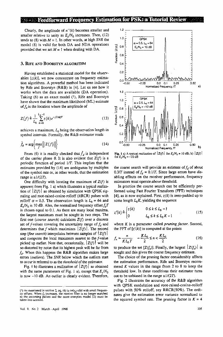
narrow estimation range for practical purposes. For example, suppose we want an estimation variance of IO-Wat EJN0 = 10 dB with NDA operation and QPSK modulation (say, with RRCR(SO%) pulses). From Fig. 3 we see that this corresponds to the MCRB for L,, = 128. The L&R estimator achieves this bound for N = &/2 = 64. However, the corresponding estimation range is *I/(MNT) = +4 . lO-VT, which is insufficient in many applications. In summary, estimation accuracy and esti- mation range are contrasting characteristics in the L&R estimator. A trade off must be sought on the basis of the actual design requirements.

Fig. 8 illustrates the accuracy of L&R algorithm for some values of L,,. The modulation is QPSK as in Fig. 7 and the estimation operation is NDA. The true frequen- cy error is zero. The parameter N is chosen equal to 16 for any L, so that the estimation range is constant and equal iO.O15/T. We see that the MCRB is achieved only for Lo = 32, corresponding to the condition N = w2. With longer observation intervals the variance is always above the MCRB. It is difficult to gather from the figure the exact position of the threshold because the curves have smoothly varying slopes. Precise threshold measurements can only be made looking for the first appearance of outliers as the SNR decreases. For exam- ple, it is found that the threshold for L,, = 32 occurs at 9 dB while for Lo = 256 it decreases to 5.5 dB. This says that the L&R algorithm can operate at low SNR provid- ed that sufficiently long observation intervals are used.

5.2. Fitz estimator

The following alternative estimator has been pro- posed by Fitz in [ 101

(36)

Note that p &T) is a bell shaped function of& which takes positive values in the range I f d l 5 I/ (MNT). Therefore, in this range, the argument of (35) equals aA4 (N + I)fdTand eq. (33) yields the correct estimate,&

Important issues about L&R algorithm are the estima- tion range and the role of the parameter N. At high SNR the estimation range is clearly *l/(MNT). Beyond these limits, in fact, p CfdT) takes negative values and this makes the estimates incorrect. Also, in [ 9 ] it is shown that the estimation variance considerably depends on N and achieves a minimum for N = L0/2. This minimum coincides with the MCRB at high SNR.

Unfortunately, choosing N = LOR may result in a too

(4) This formula is readily derived by inserting (8) into (32) and bearing in mind drat the noise-induced disturbance qr is small for SNR >> I .

Vol. Y. No. 2 March- April 1998

i NDA Operation fd = 0, N = 16

0 5 10 15 20 EdNo dB

Fig. 8 - Accuracy of L&R algorithm with NDA operation.

109

1 " ~ K M T ,,,=,

j d = - WLF) arg [ R(m)] (37)

where N is a design parameter and [w(,R] are weighting coefficients given by

6m w ( F ) = l < m l N

Itl N ( N + 1 ) ( 2 N + 1 ) An intuitive explanation of Fitz algorithm is as fol-

lows. Assuming SNR >> 1, from (34) we have

that N is chosen equal to 8 (to obtain the same estima- tion range of iO.O15/T as in Fig. 8). We see that the estimation accuracy is slightly inferior to L&R's. AS with L&R estimator, it is difficult to understand from the figure the exact position of the threshold. Searching for the SNR value corresponding to the first appearance of the outliers it turns out that the threshold decreases steadily as L, increases. For example, the threshold is 10 dB at & = 64 and7 dB at &= 256.

5.3. Lank, Reed and Pollon estimator

with

Now, suppose that 21rMmfdT is well internal to the interval -e?r so that the modulo-2~ operation is ineffec- tive in (39). Then, arg [R(m)] may be viewed as a noisy measurement of 2xMmf,T and the problem of estimat- ingfd can be approached by smoothing out the statistics (arg [ R ( m ) ] ) so as to improve the estimation process. This leads to eq. (37).

As with the L&R algorithm, the estimation range and the role of the parameter N are of interest. We have seen earlier that a critical condition to make arg [R(m)] an unbiased estimate is that 21UMmfdT be internal to the inter- val +K. As this must be true for any index m comprised between 1 and N, it follows that& must be limited within iCl/(u.INT). In conclusion, Fitz estimator has an estimation range half of L&Rs (for the same parameters M and N).

Fig. 9 illustrates the performance of the Fitz estimator with & as a parameter. Everything is as in Fig. 8 except

10-2 , I ~ , , , , , , , , , I , , , , , ,

1W

10-4

! i!

1 lo" z 10-7

10" 1, , , , ,\y 10-10

0 5 10 15 20 YNO dB

Fig. Y - Accuracy of Fitz algorithm with NDA opemion.

A considerable simplification to Fitz estimator is obtained by keeping only the last term in the sum (37). As a result we get

This is the algorithm proposed by Lank, Reed and Pollon (LRP) in [ l l ] . It turns out that its estimation range coincides with that of Fitz's (for the same N) but its performance is inferior.

5.4. Mengali and Morelli estimator

One problem with Fitz algorithm is that the modulo-2~ operation in (39) cannot be ignored at intermediate and low SNR and, in fact, it leads to significant degradations in estimation accuracy. A possible solution would be to first unwrap the sequence (arg [ R ( m ) ] ) and then insert the result into Fitz eq. (37). perhaps with different weight- ing coefficients. Mengali and Morelli (M&M) [ 121 have shown that the unwrapping process can be avoided by using the quantities (arg [R(m) R' (m - l)]} in place of (arg [ R ( m > ] ) . Their reasoning essentially follows the steps outlined with Kay's algorithm. Skipping the details, they come up with the formula

I N *d -- ~ W L M M & M ) a r g [ R ( m ) R ' ( m - I ) ] (42) * - 2 x M T ,,,=,

where

and N is a design parameter. For N = L,/2 the algorithm achieves the MCRB at high SNR [ 121.

The curves in Fig. 10 illustrate the estimation accuracy of the M&M algorithm for some values of & and QPSK modulation. NDA operation is assumed. We see that the estimator achieves the MCRB for any L, at high SNR and the threshold decreases steadily as L, increases.

5.5. Crozier and Moreland estimcitor

The following alternative method has been proposed by Crozier and Moreland (CBrM) in [ 131. Write (39) in the form

I10 ETT

1 0-2

1 0-3

10-4

0 5 10 15 20 l @ ' O

EJNo dB

Fig. 10 - Accuracy of M&M algorithm with NDA operation.

where k(m) is an integer that serves to reduce the sum 27~Mrnf~T + p(m) + 2nk(m) to the interval AX. Denoting

becomes W A = 2nfdT and v(m) 4 p(m)/(Mm), the above equation

(45)

which indicates that the left hand side may be viewed as a noisy measurement of w. In other words, the quantity arg [ R ( m ) ] / ( M m ) is an ambiguous measurement of 0, with an ambiguity quanrum of 2wl(Mm). The larger the index rn. the smaller the quantum and the more potential phase ambiguities. If the ambiguity could be resolved, an estimate of w (and eventually offd) could be derived from arg [ R ( m ) ] / ( M m ) .

Crozier and Moreland discuss the following proce- dure to overcome the ambiguity. Consider a sequence of estimates [h (mi)] associated with the following particu- lar values of the autocorrelation lag

mi=2'-1 i=1 ,2 , ..., B (46)

Eq. (45) suggests computing d (mi) as follows

(47)

where k ( q ) is a suitable integer. How can we determine k(m,) and, ultimately, compute d (mi)? Suppose that a previous unambiguous estimate 6 (mi-,) is available. Then, a reasonable value for k ( n i i ) is the one which

makes the right hand side of (47) closest to h (mi.-l). Bearing in mind that h (mi) has an ambiguity quantum of 27r/(Mmi) this leads to (for i = 2, 3,. . ., B )

or, equivalently,

& ( m i ) =

For i = 1 we have ml = 1. The corresponding estimate can be computed from (47) setting k ( 1 ) = 0, provided that w is within +n/M or, which is the same, that the frequency error f d is within 21/ (2MT) . Assuming that this is true, one starts with the,initial value

and computes the successive estimates by application of (49) up to the final estimate corresponding to i = B . In [I31 it is shown that the minimum estimation variance is achieved for B = 1 + logz (2&,/3). The degradation incurred with slightly different values is limited. how- ever. In fact in the simulations reported later we have set B = logz (f.,,) for convenience.

Fig. I I gives an idea of the estimation nnges for some algorithms discussed so far. Note that the LRP estimator has essentially the same characteristics as Fitz's and-is not shown. The ordinates yield the expectation Of f d T as obtained by simulation versus the true frequency error fdT. The modulation is QPSK with RRCR(SO%) pulses. DA operation is assumed and the SNR is 5 dB. The obser- vation length &, equals 64 and the parameter N is chosen equal to 5. We see that Fitz algorithm gives (on avenge) accurate estimates over a range slightly smaller than +lo% of l/T, The L&R algorithm has an estimation range of about +15% of 1/T and, finally, the M&M and C&M algorithms give correct results over *45% of LIT.

Fig. 12 shows the estimation accuracy of the C&M method for various observation lengths and the same

DA Operation 0.4

0.2

F --" 0.0 w

-0.2

-0.4

-0.6 -0.6 4 . 4 -0.2 0.0 0.2 0.4 0.6

Normalized Frequency Offset f,T

Fig. 11 - Expectation off,T versus/,T with various algorithms.

Vol. Y. No. 2 March - April 1998

0 5 10 15 20 Y o dB

Fig. 12 - Accuracy of C&M algorithm with NDA operation.

Algorithm

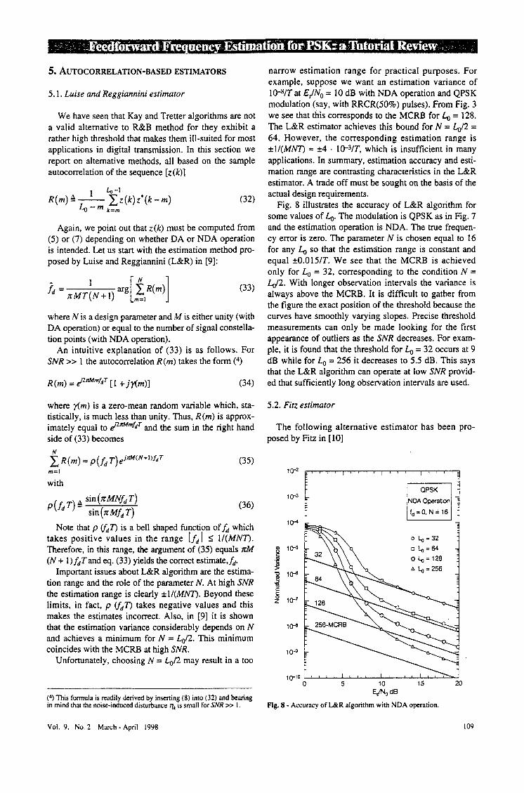
modulation format as with the M&M algorithm in Fig. 10. Although the results with the latter are slightly superior, we shall soon see that the former requires a smaller computational load.

Real Products & Additions ROM Access

6. COMPUTATIONAL COMPLEXITY

Tretter

Kay L&R

L&R (FFT-based)

One important issue that influences the choice of an estimation algorithm is its computational complexity. In

4 L , - 3

3 L 9 - 4

3 L , + 7 N - 2 + 10 (L, + N ) log, (L, + N)

4 L , ( N + 1 ) - 2 1

1

this section we address this problem and, in particular, we assess the computational load associated with the algorithms described so far. This load is expressed in terms of number of operations (real multiplications and additions) and accesses to a Read-Only-Memory (ROM). For convenience we make a distinction between DA and NDA operations. In the first instance the raw data are represented by (3, in the second they are given by (7). Note that, depending on the estimator being used, it is useful to think of z(k) as expressed in polar rather than rectangular coordinates. This is the case with estimators using arg [z (k ) ] for it obviates the need of a ROM to map z (k) into arg [z(k)l.

Fitz (FFT-based)

LRP

M&M

6.1. R& B estimator

3 L , + 5 N - 1 + lO(L,+N)lOg,(L,-N) N

8 (Lo-N)- 1 1

N (8L, - 4N - 3 ) - 2 N

We limit ourselves to the consideration of the coarse search since the fine search involves only minor extra operations. The problem is to compute KL, samples of

1 Z(f, I (see (13) ) via an FFI'. As is known [ 141, the FIT involves about KL, log, (KL0)/2 complex multiplica- tions, KL, log, (KL,,) complex additions and K L , mod- ulus extractions. This leads to the R&B line in Table 1 with p = 1. In writing this line we have taken into ac- count the fact that a complex multiplication corresponds to four (real) multiplications and two (real) additions, each modulus extraction requires two multiplications and one addition and searching for the maximum in the set [ I Z(Jn) 1 ] requires KL, comparisons. All these opera- tions have been put together since in a DSP implementa- tion they have approximately the same weight.

M&M(FFT-based) 1 C&M

Table 1 - Computational load with DA operation

3L9 + 6 N - 2 + 10 (4 + N) log2 (4 + N)

8 (&B-2') + 2 8 + 5

N

B

112 Ell-

Some saving in the FFT calculation is obtained by eliminating operations on zeros, which is commonly referred to as pruning [ 151. It can be shown that pruning reduces the number of multiplications and additions by a factor

-

Algorithm Real Products & Additions

R&B KLo [4 + 2.5 P log2 (K4,)I

Tretter 4L0 - 3

Kay 3L0 - 4

L&R

L&R (FFT-based)

Fitz

Fitz (FFT-based)

LRP 3(L,-N)-1

0.5N (6Lo - 3N + 1) - 2

3Lo + 7 N - 2 + 7.5 (L, + N) log2 (L, + N)

0.5N (6L, - 3 N - 3 ) - 1

3Lo + 5N - 1 + 7.5 (L, + N) log, (Lo + N)

log, ( K ) + 2(1/ K - 1) p = l - log2 (KL,,)

ROM Access

K L , P log, (al)

N (2L, - N - 1) + 1

1 +(43+N)IO&(L,+N)

N (2LO - N)

N + (L, + N) log, (Lo + N)

2 ( L n - N ) + 1

Correspondingly the R&B line becomes as indicated in Table 1 for a generic p. Note that for K = 2 we have p = 1 and the pruning does not allow any computational saving.

M&M(FFT-based)

C&M

tions are required in ( 1 9). This yields the Tretter lines in Tables 1 and 2.

3L0 + 6 N - 2 + 7.5 (Lo + N) log? (Lo + N) N + + N) log2 (L, + N )

3 ( 4 B - Z B ) + 2B 2 (L"B - 28) + B + 2

6.3. Kay estimator

Again, we use the data arg [ ~ ( k ) ] . As is seen from (23), the calculation of the set arg [z(k) Z* (k - l)], 1 I k 5 L,,, requires L, - 1 additions while the right hand side in (26) involves L, - 1 products and & - 2 additions. This leads to the Kay line in Tables 1 and 2.

6.4. LdiR estimator

6.4.1. DA OPERATION

6.1.2. NDA OPERATION

Recalling that '1 z(k) I = 1 , the generic term in (13) may be written as

So, starting from (arg [z(k)]; k = 0, 1 ,..., Lo - 1 }', we need one addition and two ROM accesses to compute z ( k ) e-j*WT (for sin ( x ) and cos(x)). Therefore the pruned FFT requires 5KL0 p log, (KL0)/2 additions and K L , p log, (KL,) ROM accesses. Adding the operations for modulus extraction and maximization over the set [ I ZUn) I ] produces the line R&B in Table 2.

6.2. Tretter estimator

Using the data arg [z(k)], there are 2 (L,, - 1) additions involved in (21). Also, L,, - 1 additions and L, multiplica-

Luise and Reggiannini [9 ] have proposed a clever method to compute fd that significantly reduces the computational load. The interested reader is referred to their paper for details. The resulting complexity is indi- cated in the L&R line in Table 1. Alternatively, the computation of the set [R(m)], m = 1, 2, ... N, can be car- ried out in the frequency domain through the following steps [ 14, p. 5561:

i) form an (Lo + N)-point sequence by adding N zeroes to [ ~ ( k ) ]

ii) compute the (Lo + N)-point Discrete Fourier Transform (DFT)

Z(n) =

k = O

Table 2 - Computational load with NDA operation

I NDA Operation I

Vol. 9, No. 2 March - April I Y Y Y I I3

iii) compute the (Lo + N)-point inverse DFT of I z(n) I *

1 h + N

y ( m ) = -.

iv) finally, compute R(m) as

The FIT is used to efficiently perform operations ii) and iii). The resulting complexity is indicated in the L&R (FFT-based) line in Table 1.

6.4.2. NDA OPERATION

It turns out that the procedure described in [9] is not useful with NDA operation. Instead, the following approach can be used. From the formula

additions and N ROM accesses. In both cases the final calculation off, involves N further multiplications and N- 1 additions.

6.5.2. NDA OPERATION

Writing t ( k ) z* (k - m ) as in (56) allows us to com- pute the set [8 (m)] through N (64 , - 3 N - 7 ) / 2 additions and N (2L, - N) ROM accesses in the time domain. Alternatively, in the frequency domain we need 2 (L, + N) [l + log, (L, + N)] products, (L, + N) [l + 5.5 logl (L, + N ) ] additions and N + (L,, + N) log2 (L, + N) ROM accesses. The steps to compute f, remain the same as with DA operation.

6.6. U P estimator

The LRP estimator can be treated as a special case of Fitz method. Here, however, the FFT-based method is not useful since only one autocomelation is needed.

6.7. MQM estimator

From (32) and (58) we have

arg [R(m) R” (rn - I ) ] = [ O (m) - 8 (m - l)Jfn (59 ) it is clear that the computation of z ( k ) zf ( k - m) requires one addition and two ROM accesses (for sin(x) and cos(x)). Thus, the calculation of the set [R(m)] , m = 1. 2, ..A, in the time domain involves 2N multiplications, N (64, - 3N - 7 ) / 2 additions and N (2L, - N - I ) ROM accesses. Viceversa, in the frequency domain (FFT-based method), we need 2 (4, + 2N) + 2 (&, + N) log, (4, + N) products, L, + N + 5.5 (4 + N) log, (&, + N) additions and (4 + N))0g2 (&, + N) ROM accesses. The final com- putation of f, from (33) requires 2 ( N - 1) further addi- tions and one ROM access.

6.5. Fitz estimator

So, once the sequence [8 (m) ] is computed (see Fitz estimator), the right hand side of (42) requires N multi- plications and 2 (N - 1) additions.

6.8. C&M estimator

6.8.1. DA OPERATION

The computation of the set (arg [ R ( m i ) ] } (mi = 2I-l and i = I , 2.. . ., B) requires & B + I + 28 complex prod- ucts, (&, - I ) B + 1 - 2B complex additions and B ROM accesses. Also, the recursions (49) involve 2 ( B - 1) multiplications and additions.

6.5.1. DA OPERATION 6.8.2. NDA OPERATION

Bearing in mind the definition (32) we can rewrite the Fitz estimator in the form

(57)

Then, the computation of the set [8 (m)] in the time domain requires 2N (2L, - N - 1) multiplications. 2N (24, - N - 2) additions and N ROM accesses. In the fre- quency domain, viceversa. i t needs 2 ( L , + N) [ I + 2 log, (4) + N)] products. (& + M [I + 6 log? (4, + N)1

The computation of the set (arg [R(m, ) ] ) requires 3 (L, B + 1 - 28) - 2B additions and 2 (& B + 1 - 2B) + B ROM accesses while the steps involved in (49) remain the same. The FIT-based method has not been consid- ered since only few autocorrelations are needed.

6.9. COMPAFWONS

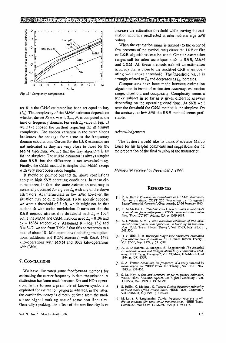
Fig. 13 shows complexity comparisons between some of the above estimation schemes with DA operation. Each curve gives the total number of multiplications and additions as a function of the observation length 4,. A pruning factor of K = 4 has been chosen with the R&B algorithm and three different values for N have been used with the M&M method. Finally, the pamme-

l I4

!

2 3 4 5 6 7

Kav i

Lag2 Ll Fig. 13 - Complexity comparisons.

__ 8 9 10 11 12

ter B in the C&M estimator has been set equal to log, (Lo). The complexity of the M&M estimator depends on whether the set R ( m ) , m = 1, 2 ,..., N , is computed in the time or frequency domain. For each Lo value in Fig. 13 we have chosen the method requiring the minimum complexity. The sudden variation in the curve slopes indicates the passage from time to the frequency domain calculations. Curves for the L&R estimator are not indicated as they are very close to those for the M&M algorithm. We see that the Kay algorithm is by far the simplest. The M&M estimator is always simpler than R&B, but the difference is not overwhelming. Finally, the C&M method is simpler than M&M except with very short observation lengths.

It should be pointed out that the above conclusions apply to high SNR operating conditions. In these cir- cumstances, in fact, the same estimation accuracy is essentially obtained for a given L, with any of the above estimators. At intermediate or low SNR, however, the situation may be quite different. To be specific suppose we want a threshold of 3 dB, which might not be that outlandish with coded modulation. It turns out that the R&B method attains this threshold with L, = 1024 while the M&M and C&M methods need L, = 8 196 and Lo = 16384 respectively. Assuming B = log, (Lo) and N = &/2, we see from Table 2 that this corresponds to a total of about 18 1 kilo-operations (including multiplica- tions, additions and ROM accesses) with R&B, 1472 kilo-operations with M&M and 1065 kilo-operations with C&M.

7. CONCLUSIONS

We have illustrated some feedforward methods for estimating the carrier frequency in data transmission. A distinction has been made between DA and NDA opera- tion. In the former a preamble of known symbols is exploited for estimation purposes whereas, in the latter, the canier frequency is directly derived from the mod- ulated signal making use of some non linearity. Generally speaking, the effect of the non linearity is to

Vol. Y. No. 2 March - April 1998

increase the estimation threshold while leaving the esti- mation accuracy unaffected at intermediateAarge SNR values.

When the estimation range is limited (to the order of few percents of the symbol rate) either the LRP or F iu or L&R algorithms can be used. Greater estimation ranges call for other techniques such as R&B, M&M and C&M. All these methods exhibit an estimation accuracy that is close to the modified CRB when oper- ating well above threshold. The ‘threshold value is strongly related to L, and decreases as Lo increases.

Comparisons have been made between estimation algorithms in terms of estimation accuracy, estimation range, threshold and complexity. Complexity seems a tricky subject in so far as it gives different answers depending on the operating-conditions. At SNR well over the threshold the C&M method is the simplest. On the contrary, at low SNR the R&B method seems pref- erable.

Acknowledgements

The authors would like to thank Professor Marco Luke for his helpful comments and suggestions during the preparation of the final version of the manuscript.

Manuscript received on November 3, I997.

REFERENCES

R. A. Hams: Transinission considerations for LAN interconnec- tion by satell i te. COST 226 Workshop on “Integrated Spacflerrestrial Networks”, G n z , Austria. 25-26 February 1993.

F. Ananasso. G. Pennoni: Clock synchronorrs mulricarrier demotlrilator for nrirltifreqnency T D M A communications satel- lites. “Proc. ICC’90’. Atlanta, GA, p. 1059-1063. A. J. Viterbi. A. M. Viterbi: Nonlineur estimation of PSK-mod- tiluted currier phuse with application to burst digital transmis- sion. “IEEE Trans. Inform. Theory”. Vol. IT-29, July 1983. p. 543-550. D. C. Rife, R. R. Boorstyn: Single-tone parameter estimution from discrete-time observations. “IEEE Trans. Inform. Theory”, Vol. IT-20. Sept. 1974, p. 591-598. A. N. D’Andrea, U. Mengali, R. Reggiannini: The modified Cramer-Rtro bound and Its applications to synchronization prob- lems. “IEEE Trans. Commun.”. Vol. COMJZ, Feb./MarcNApril

S. A. Tretter: Esrirntrtirrg the frequency of a noisy sinusoid by linear regression. ”IEEE Trans. Inf. Theory”. Vol. IT-3 I, Nov.

S. M. Kay: A fast curd accurate single frequency estimator. W E E Trans. Acoustic. Speech and Signal Processing”. Vol. ASSP-37. Dec. 1989. p. 1987- 1990. S . Be I I i n i. C. Mo I i nari , G. Tanara: Digittrl Jreqrrenc:v esriinution in biirst inode QPSK mrnsrtrission. “IEEE Trans. Commun.”.

M. Luisz. R. Reggiannini: Currier jreqiienc:v recover?. in (111- c f i , ~ i r t r l iirot1em.s fbr birrst-inode rruirsmis.sionu. ”IEEE Trans. Commun.”. Vol. COM-43. March 1995. p. 1169-1 178.

1994, p. 1391-1399.

1985. p. 832-835.

Vol. COM-38. July 19‘90. p. 959-961.

I I5

M. P. Fitz: Further results in the fast estimation of a single re quency. “IEEE Trans. Commun.”. Vol. COM-42. March 19/94. G. W. Lank. 1. S. Reed, G. E. Pollon: 4 semicoherent derecrion and Doppler estimation statistic. IEEE Trans. Aerosp. Electron. Syst.”. Vol. AES-9, March 1973. p. 151-165. U. Mengali, M. Morelli: Dat;-aided frequency estimation burst digital transmission. IEEE Trans. Commun.”. & COM-45. Jan. 1997. p. 23-25.

[ 131

p. 862-864.

“41

[I51

S. Crozier, K . Moreland Performance of u simple delay-multi- ply-averaeqe technique for frequency estimation. Canadian Conf. on Electrical and Computer Eng., Toronto, Canada, paper WM-

A. V. Oppenheim, R. W. Schafer: D i g i d signal Processing. Prentice-Hall, Englrwwd Cliffs, NJ, 1979. J. D. Markel: FFTpruning. “IEEE Tnns. Audio Electmacoustic”.

10.3, Sept. 13-16. 1992.

VOI. AU-19, D ~ C . 1971, p. 305-311.

I16