Feeding the Smart Phone���The Limits of Spatial Reuse in Picocells

Upamanyu Madhow

ECE Department, University of California, Santa Barbara

Work actually done by Dinesh Ramasamy

The wireless industry who cried wolf

•  After years of hype, exponential growth in wireless data hits with a vengeance

2  

Irreversible trends

•  iPhone/Android, Pandora/Spotify, Netflix/Amazon

•  Tiered pricing can only go so far – Mice are becoming elephants

3  

How to feed the smart phone? •  Need exponential growth in network capacity •  Possible answers

– Spatial reuse: cell size reduction

– Offload to WiFi (or co-opt WLAN into cellular network via femtocell)

– Advanced cross-layer techniques

•  Today’s talk: how far can picocells take us? can we provide wire-like determinism? how decentralized can resource management be?

how much does network MIMO help? 4  

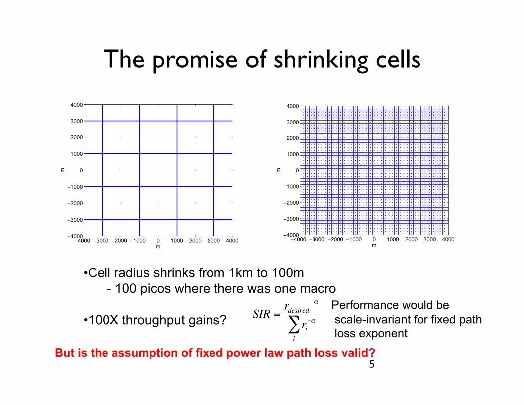
The promise of shrinking cells

!!""" !#""" !$""" !%""" " %""" $""" #""" !"""!!"""

!#"""

!$"""

!%"""

"

%"""

$"""

#"""

!"""

&

&

!!""" !#""" !$""" !%""" " %""" $""" #""" !"""!!"""

!#"""

!$"""

!%"""

"

%"""

$"""

#"""

!"""

&

&

5  

• Cell radius shrinks from 1km to 100m -  100 picos where there was one macro

• 100X throughput gains?

€

SIR =rdesired

−α

ri−α

i∑

Performance would be scale-invariant for fixed path loss exponent

But is the assumption of fixed power law path loss valid?

Revisiting path loss models

6

The perils of power laws

•  d-α predicts path loss locally (not for all d) –  Depends on distance relative to geometry of TX, RX,

environment •  Small cells (e.g., lamppost based base stations)

–  Signal from serving BS is near-LOS α=2 a good fit

–  Is α=2 a good guess for interference from other cells? •  Yes for nearby cells (i.e., for aggressive reuse)

•  But not for far-away cells (blocked by buildings)

7  

The fourth power model: LOS & ground reflection

8  

•  Power law “regime change” reported in measurements; justified via ground reflections

M. J. Feuerstein, K. L. Blackard, T. S. Rappaport, S. Y. Seidel, and H. H. Xia, “Path loss, delay spread, and outage models as functions of antenna height for microcellular system design,” ITVT ’94.

PL(d) =

�−20 log10 (4πd/λc) d ≤ df−20 log10 (4πdf/λc)− 40 log10 (d/df ) d > df

At 1.9GHz, Rx height 1.7m, predicted regime change at: Tx mounted 13.2m high is 573m Tx mounted 3.7m high is 159m

Fresnel  breakpoint  

df ≈ 4hthr

λc

hthr

d

Second power + exponential: multi-slit waveguide

•  Urban scenarios, along the street with BS

•  Channel model:

•  Random slit positions give exp falloff

•  Breakdown distance depends on environment

9  

PL(d) = −20 log10

�4πd

λc

�− 4.3ηd

η−1 ≈ 150m− 500m

N. Blaunstein, R. Giladi, and M. Levin, “Characteristics’ prediction in urban and suburban environments,” ITVT ’98.

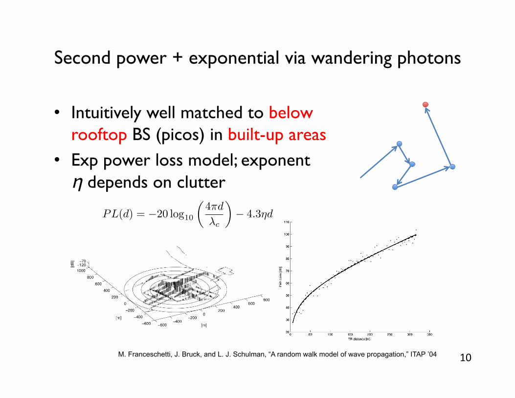
Second power + exponential via wandering photons

•  Intuitively well matched to below rooftop BS (picos) in built-up areas

•  Exp power loss model; exponent η depends on clutter

10  

PL(d) = −20 log10

�4πd

λc

�− 4.3ηd

M. Franceschetti, J. Bruck, and L. J. Schulman, “A random walk model of wave propagation,” ITAP ’04

Second power + exponential as a unified model?

11  

B. Van Laethem, F. Quitin, F. Bellens, C. Oestges, and P. De Doncker, "Correlation for multi-frequency propagation in urban environments,” Progress In Electromagnetics Research Letters, ’12.

!"#

!"$

!!%"

!!&"

!!'"

!!$"

!!#"

!!!"

!!""

!("

)*+,-./0123

4

4

!5""678420-+9:020.,+

0;<42=>0?4@*,44!!!4A4#''2

<=B0:4?-B4@*,44"A!'C"D$&

Exponen:al  model  fits  measurement  data  well  over  a  much  larger  range  than  any  single  power  law  

Limits of spatial reuse

12

Model

•  Channel model – Second power + exp path

loss model – phase due to LOS beam

•  Square grids; regular reuse; random user locations

•  Carrier frequency 2GHz 13  

h(d) = 10PL(d)/20ej2πd/λc

PL(d) = −20 log10

�4πd

λc

�− 4.3ηd

Reuse ¼

! "! #! $! %!"!

!$

"!!#

"!!"

"!!

&'()

*+','-./'!'&'0

'

'

/1231'"4'-5677'8177

/1231'"9%4'-5677'8177

/1231'"9:4'-5677'8177

/1231'"4';6+<1'8177

/1231'"9%4';6+<1'8177

/1231'"9:4';6+<1'8177

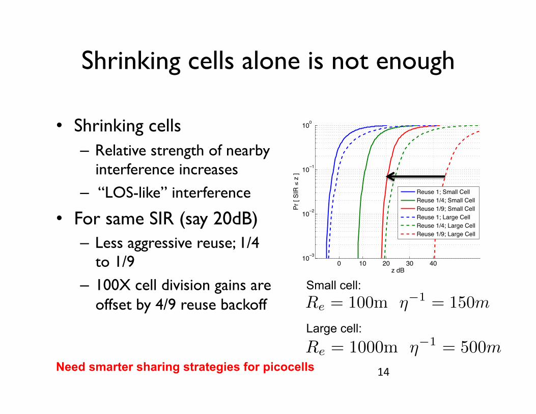
Shrinking cells alone is not enough

•  Shrinking cells –  Relative strength of nearby

interference increases

–  “LOS-like” interference

•  For same SIR (say 20dB) –  Less aggressive reuse; 1/4

to 1/9

–  100X cell division gains are offset by 4/9 reuse backoff

14  

Re = 100m η−1 = 150mSmall cell:

Large cell: Re = 1000m η−1 = 500m

Need smarter sharing strategies for picocells

Design approach for small cells

•  High peak rates – high bandwidth efficiency, high SIR target

•  Quasi-deterministic performance – Towards zero outage – Feasible in near-LOS environments

•  Must coordinate with nearby picocells – Single interferer can wipe you out in near-LOS

environment – But naïve orthogonalization is too costly

•  “Far-away” picocells set interference floor 15  

A Scalable Architecture

16  

r

R r= cell radius R= coordination radius (no coordination with cells outside coordination radius)

Tagged cell

Nearby interference causes too much damage in near-LOS environments must coordinate with neighboring cells Cells outside coordination region set interference floor Strategy inside coordination region affects interference floor

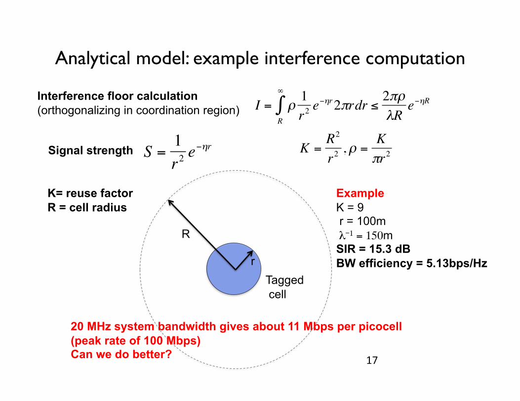
Analytical model: example interference computation

17  

r

R

Tagged cell

€

I = ρ1r2e−ηr2πrdr

R

∞

∫ ≤2πρλR

e−ηR

K =R2

r2, ρ =

Kπr2

Interference floor calculation (orthogonalizing in coordination region)

Signal strength

€

S =1r2e−ηr

K= reuse factor R = cell radius

Example K = 9 r = 100m λ-1 = 150m SIR = 15.3 dB BW efficiency = 5.13bps/Hz

20 MHz system bandwidth gives about 11 Mbps per picocell (peak rate of 100 Mbps) Can we do better?

How to get back spatial reuse in picocells

•  Why is spatial reuse impaired in picocells? – Near-LOS interference can wipe you out

– But naïve orthogonalization really hurts capacity

•  Can we reduce nearby interference? – Beamforming

•  Can we turn nearby “interference” into “desired signal”? – Collaborative beamforming (CoMP)

18  

Base station antenna arrays

19  

Diameter = λc = 15cm

!"

#$"

%"

#&"

'"

#("

$#"

!""

$)"

!!"

$*" "

!!$+$)",-./011.234567+$"",-.8

3+&

!"

#$"

%"

#&"

'"

#("

$#"

!""

$)"

!!"

$*" "

!!$+$)",-./011.234567+$"",-.8

3+*

4 element array

8 element array

Focus power when transmitting

! "! #! $! %!"!

!$

"!!#

"!!"

"!!

&'(()*+,-./0"!!1))!!"0"2!1

3),4

5*6789)")3),4:

)

)

;+0"<)9'./')"=%

;+0%<)9'./')"=%

;+0><)9'./')"=%

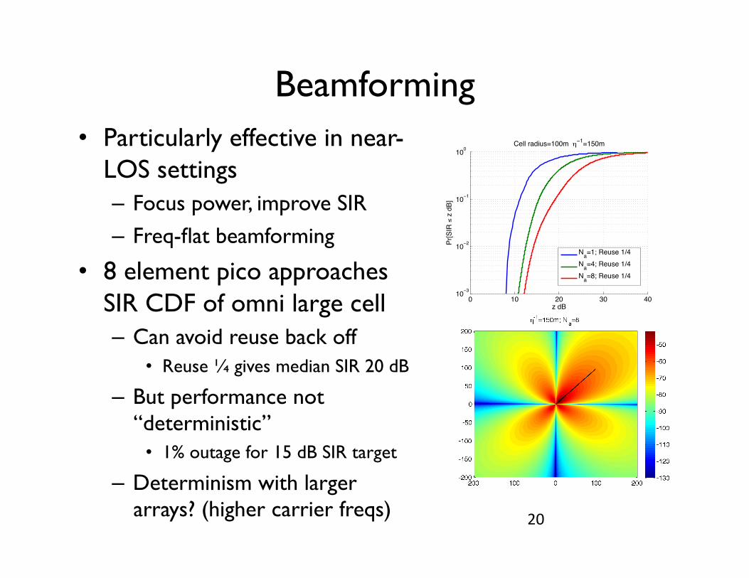
Beamforming •  Particularly effective in near-

LOS settings –  Focus power, improve SIR

–  Freq-flat beamforming

•  8 element pico approaches SIR CDF of omni large cell –  Can avoid reuse back off

•  Reuse ¼ gives median SIR 20 dB

–  But performance not “deterministic”

•  1% outage for 15 dB SIR target

–  Determinism with larger arrays? (higher carrier freqs) 20  

CoMP Beamforming

10 15 20 25 30 35 4010 2

10 1

100

z dB

Pr[S

IR

z d

B]

Cell radius=100m 1=150m

Reuse 1/4; Na=1; 4BSReuse 1/4; Na=4; 4BSReuse 1/4; Na=8; 4BS

21  

- 8 Element array with CoMP better than large cell reuse ¼ - Performance getting more “deterministic”

Define “virtual cells” based on cluster of collaborating BS

Reuse 1/4

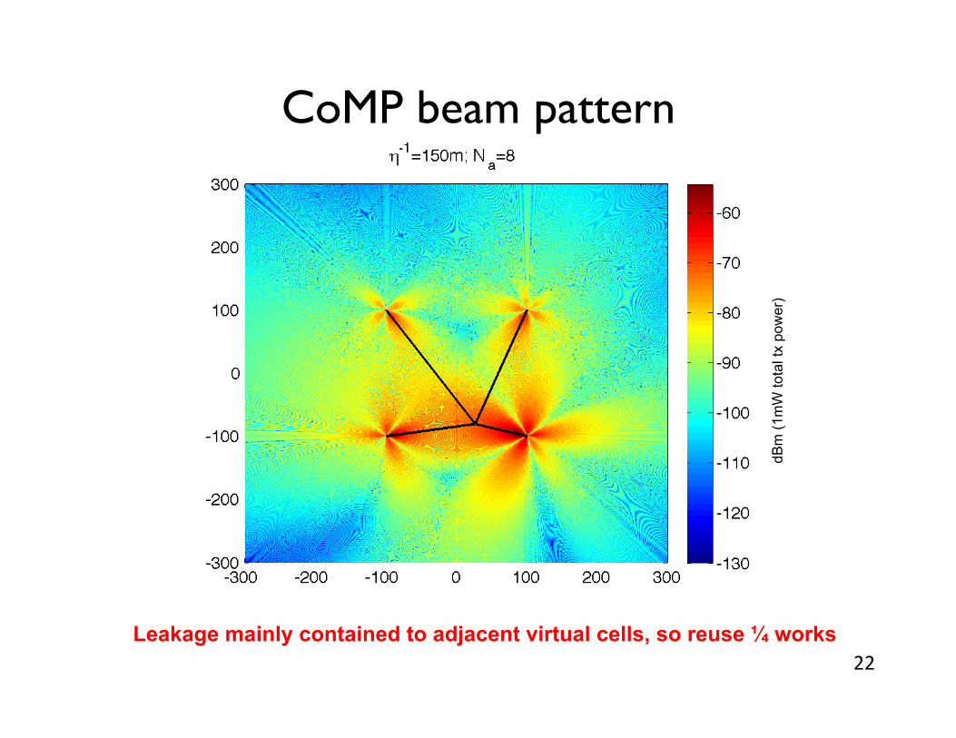
CoMP beam pattern

22  Leakage mainly contained to adjacent virtual cells, so reuse ¼ works

dBm

(1m

W to

tal t

x po

wer

)

CoMP Multiplexing

•  Serve 2 users per virtual cell –  “Effective reuse” rate ½ –  SIR > 15dB

•  1.5X better than large cell (omni; naïve) per cell –  150X network capacity

gain

0 5 10 15 20 25 30 35 4010 2

10 1

100

z dBPr

[SIR

z

dB]

Cell radius=100m 1=150m

Reuse 1/2; Na=1; 4BSReuse 1/2; Na=4; 4BSReuse 1/2; Na=8; 4BS

23  

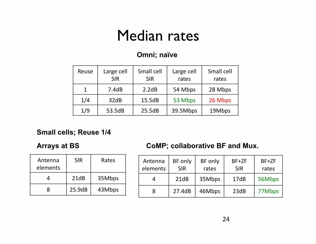
Median rates

24  

Reuse   Large  cell  SIR  

Small  cell  SIR  

Large  cell  rates  

Small  cell  rates  

1   7.4dB   2.2dB   54  Mbps   28  Mbps  

1/4   32dB   15.5dB   53  Mbps   26  Mbps  

1/9   53.5dB   25.5dB   39.5Mbps   19Mbps  

Omni; naïve

Antenna  elements  

SIR   Rates  

4   21dB   35Mbps  

8   25.9dB   43Mbps  

Small cells; Reuse 1/4

Antenna  elements  

BF  only  SIR  

BF  only  rates  

BF+ZF  SIR  

BF+ZF  rates    

4   21dB   35Mbps   17dB   56Mbps  

8   27.4dB   46Mbps   23dB   77Mbps  

CoMP; collaborative BF and Mux. Arrays at BS

Three nines (0.1% outage) rates

25  

Reuse   Large  cell  SIR  

Small  cell  SIR  

Large  cell  rates  

Small  cell  rates  

1   -­‐4.1dB     -­‐5.3dB     9.4Mbps   7.5Mbps  

1/4   20dB   8dB   33.3Mbps   14.3Mbps  

1/9   40dB   18dB   29.5Mbps   13.3Mbps  

Omni; naïve

Antenna  elements  

SIR   Rates  

4   11dB   19Mbps  

8   12dB   21Mbps  

Antenna  elements  

BF  only  SIR  

BF  only  rates  

BF+ZF  SIR  

BF+ZF  rates    

4   13.5dB   23Mbps   7.5dB   27Mbps  

8   19dB   32Mbps   14.5dB   49Mbps  

Small cells; Reuse 1/4

CoMP; collaborative BF and Mux. Arrays at BS

What we have learnt •  Fixed power law models can be misleading •  2nd power/exponential promising model

–  Interference is “amplified” as we shrink cell size

– Naïve orthogonalization gives away scaling gains – Local coordination is critical

•  Beamforming can help – Still need to enforce reuse

•  Collaborative beamforming can really help! – Requires very tight coordination with neighbors – Still need to enforce reuse

26  

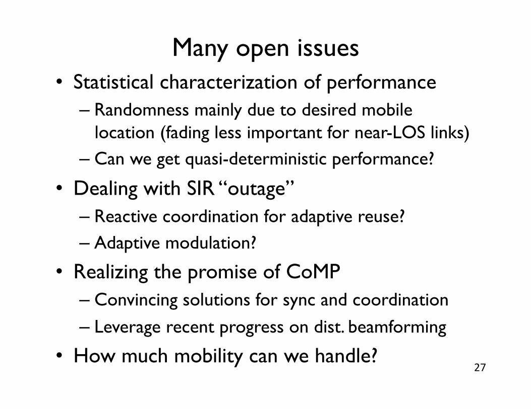
Many open issues •  Statistical characterization of performance

– Randomness mainly due to desired mobile location (fading less important for near-LOS links)

– Can we get quasi-deterministic performance?

•  Dealing with SIR “outage” – Reactive coordination for adaptive reuse? – Adaptive modulation?

•  Realizing the promise of CoMP – Convincing solutions for sync and coordination

– Leverage recent progress on dist. beamforming

•  How much mobility can we handle? 27  

A Couple of Asides

The Role of 60 GHz

28

Beamforming to the limit

•  Very large arrays at picocellular basestations give reuse one without CoMP

•  60 GHz to the mobile? – Attractive once WiGig makes it into smart phones

•  Host of issues – Adapting large arrays (promising recent progress)

– Shadowing – Mobility management

29  

Compressive Adaptation of 1000 element arrays

Compressive measurements

Spatial channel estimation

Weight computation Quantized beamsteering

Randomized weights

Optimized weights

Es:ma:on  

Beamforming  

Ramasamy, Venkateswaran, Madhow, ITA 2012

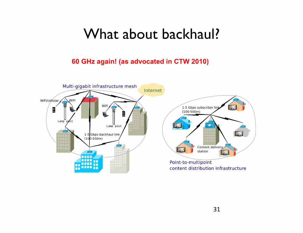
What about backhaul?

31  

60 GHz again! (as advocated in CTW 2010)

Determinism in the backhaul

32  

wall LoS

ground

Deterministic diversity for sparse multipath (Zhang and Madhow, recent results)

Determinism: steep rise in CDF of average channel power gain

Freq diversity enough if BW > 1/(smallest differential delay)

Spatial diversity provides determinism even if BW < 1/(smallest differential delay)

Final thoughts •  Yes we can!

–  the smart phone need not go hungry

•  But it will need work – Tight coordination between neighbors for CoMP – Decentralized, scalable protocols for resource

sharing and mobility tracking

– MultiGigabit backhauls – 60 GHz to the mobile

•  All good news for the wireless researcher! – Redoing digital cellular 20 years later

33