FINITE ELEMENT ANA Siddhartha Ghosh* and * Assistant Professor, ** Res * Assistant Professor, ** Res Department of C Department of C Indian Institute of Te Indian Institute of Te ALYSIS IN ABAQUS Swapnil B. Kharmale** search Scholar (PhD Student ) search Scholar (PhD Student ) Civil Engineering Civil Engineering echnology, Bombay echnology, Bombay
Transcript
FINITE ELEMENT ANALYSIS IN
Siddhartha Ghosh* and * Assistant Professor, ** Research Scholar (PhD Student )* Assistant Professor, ** Research Scholar (PhD Student )
Department of Civil EngineeringDepartment of Civil EngineeringIndian Institute of Technology, BombayIndian Institute of Technology, Bombay
ELEMENT ANALYSIS IN ABAQUS
Siddhartha Ghosh* and Swapnil B. Kharmale** * Assistant Professor, ** Research Scholar (PhD Student )* Assistant Professor, ** Research Scholar (PhD Student )
Department of Civil EngineeringDepartment of Civil EngineeringIndian Institute of Technology, BombayIndian Institute of Technology, Bombay
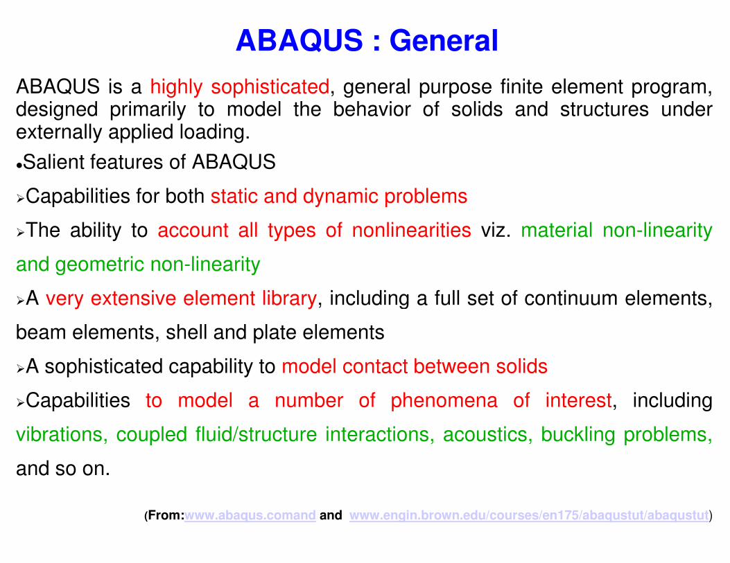
ABAQUS : General
ABAQUS is a highly sophisticated, generaldesigned primarily to model the behaviorexternally applied loading.
�Salient features of ABAQUS
�Capabilities for both static and dynamic
�The ability to account all types of nonlinearities
and geometric non-linearity
�A very extensive element library, including
beam elements, shell and plate elements
�A sophisticated capability to model contact
�Capabilities to model a number of
vibrations, coupled fluid/structure interactions,
and so on.
(From:www.abaqus.comand and www.engin.brown.edu/courses/en
ABAQUS : General
general purpose finite element program,behavior of solids and structures under
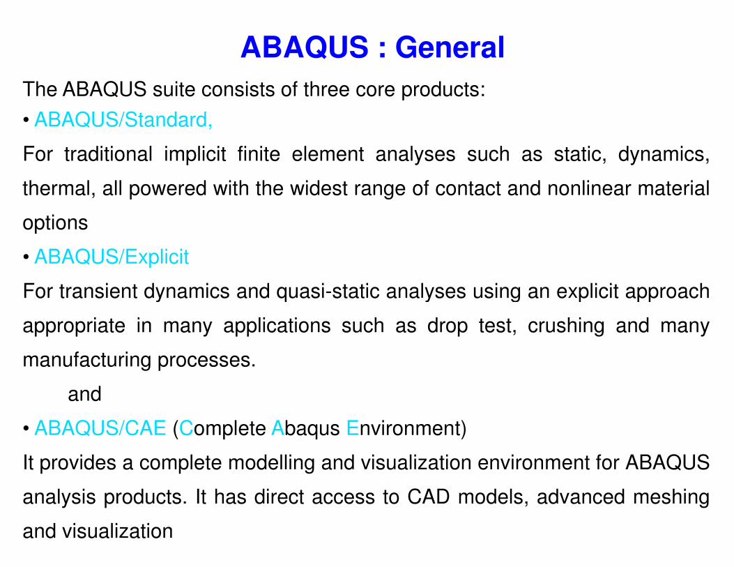
For transient dynamics and quasi-staticFor transient dynamics and quasi-static
appropriate in many applications such
manufacturing processes.
and
• ABAQUS/CAE (Complete Abaqus Environment)
It provides a complete modelling and visualization
analysis products. It has direct access
and visualization
ABAQUS : General
The ABAQUS suite consists of three core products:
analyses such as static, dynamics,
range of contact and nonlinear material
static analyses using an explicit approachstatic analyses using an explicit approach
such as drop test, crushing and many
nvironment)
visualization environment for ABAQUS
access to CAD models, advanced meshing
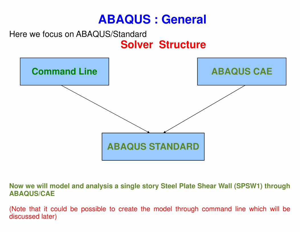
ABAQUS : GeneralHere we focus on ABAQUS/Standard
Command Line
Solver Structure
ABAQUS STANDARD
Now we will model and analysis a single storyABAQUS/CAE
(Note that it could be possible to create thediscussed later)
ABAQUS : General
ABAQUS CAE
Solver Structure
ABAQUS STANDARD
story Steel Plate Shear Wall (SPSW1) through
the model through command line which will be
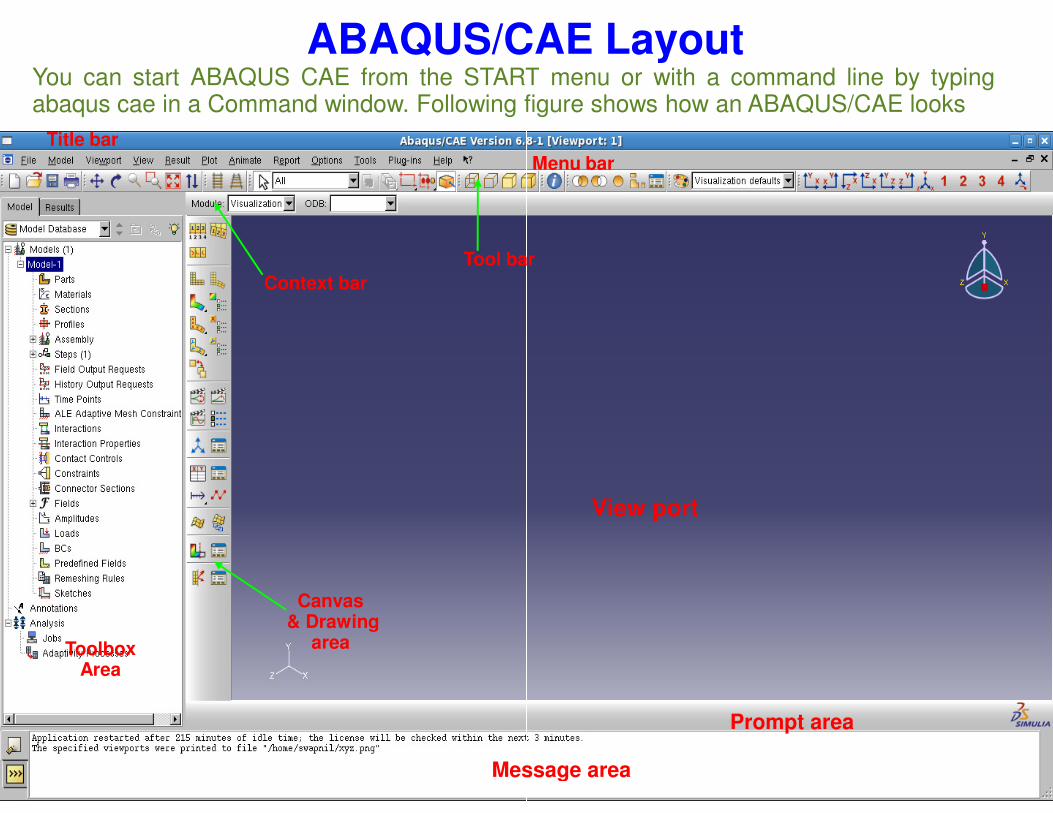
ABAQUS/CAE Layout
Title bar
Context bar
Tool bar
You can start ABAQUS CAE from the STARTabaqus cae in a Command window. Following figure
Message area
Canvas& Drawing
areaToolbox Area
ABAQUS/CAE Layout
Menu bar
Tool bar
START menu or with a command line by typingfigure shows how an ABAQUS/CAE looks
View port
Message area
Prompt area
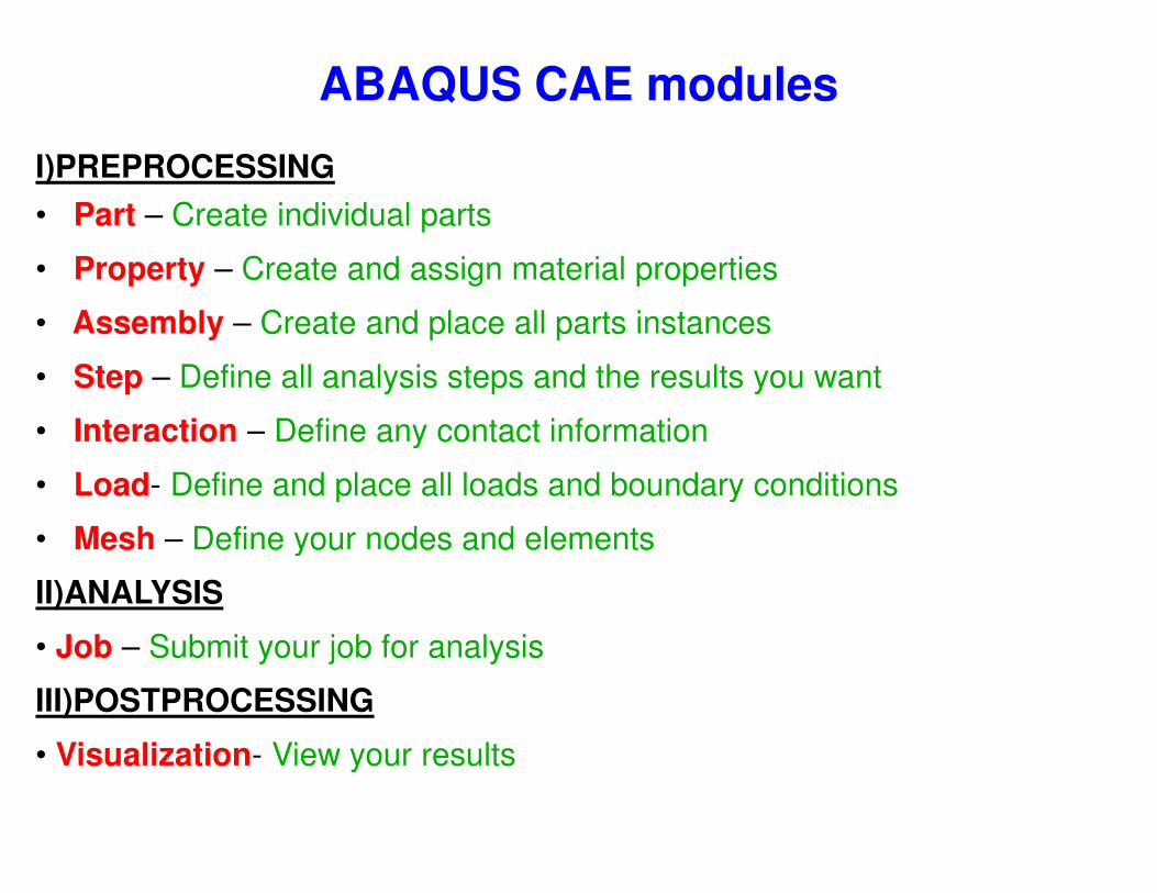
ABAQUS CAE modules
I)PREPROCESSING
• Part – Create individual parts
• Property – Create and assign material properties
• Assembly – Create and place all parts instances
• Step – Define all analysis steps and the results you want
• Interaction – Define any contact information• Interaction – Define any contact information
• Load- Define and place all loads and boundary conditions
• Mesh – Define your nodes and elements
II)ANALYSIS
• Job – Submit your job for analysis
III)POSTPROCESSING
• Visualization- View your results
ABAQUS CAE modules
Create and assign material properties
Create and place all parts instances
Define all analysis steps and the results you want
Define any contact informationDefine any contact information
Define and place all loads and boundary conditions
Define your nodes and elements
3-Dimensional FEM Problem(Pushover Analysis of SPSW)
�To start learning ABAQUS CAEsingle story Steel Plate Shearincludes geometric nonlinearityduring fabrication). The specimenload (Non-linear static pushover analysis)
�Problem Statement
To find the ultimate load carrying
story steel plate shear wall (SPSW
analysis.
Dimensional FEM Problem(Pushover Analysis of SPSW)
we will work through modelling aWall (SPSW1) specimen which(initial out-of-plane deformationsis subjected to monotonic lateral
analysis)
carrying capacity (Lateral load) of single
(SPSW1) by non-linear static push over
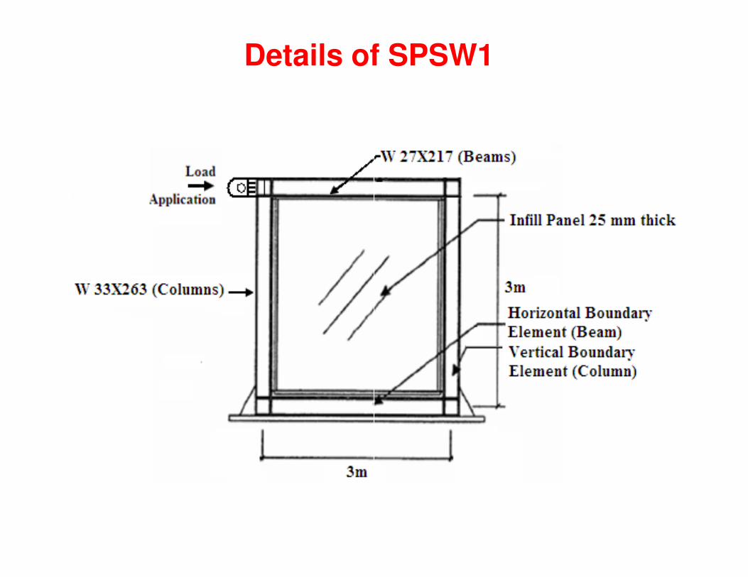
Details of SPSWDetails of SPSW1
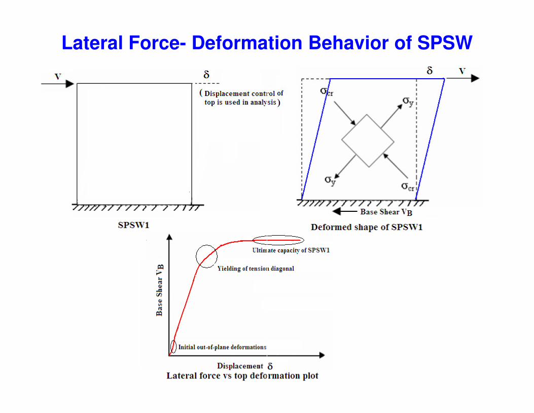
Lateral Force- Deformation Deformation Behavior of SPSW
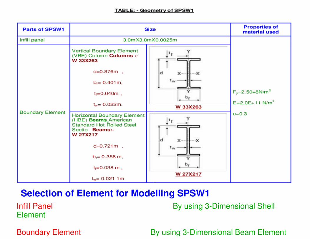
Selection of Element for Modelling SPSW
Infill Panel Element
Boundary Element By using
Selection of Element for Modelling SPSW1
By using 3-Dimensional Shell
By using 3-Dimensional Beam Element
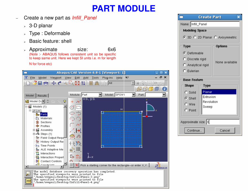
PART MODULE− Create a new part as Infill_Panel
� 3-D planar
� Type : Deformable
� Basic feature: shell
� Approximate size: 6x6(Note :- ABAQUS follows consistent unit so be specificto keep same unit. Here we kept SI units i.e. m for length
N for force etc)
PART MODULE
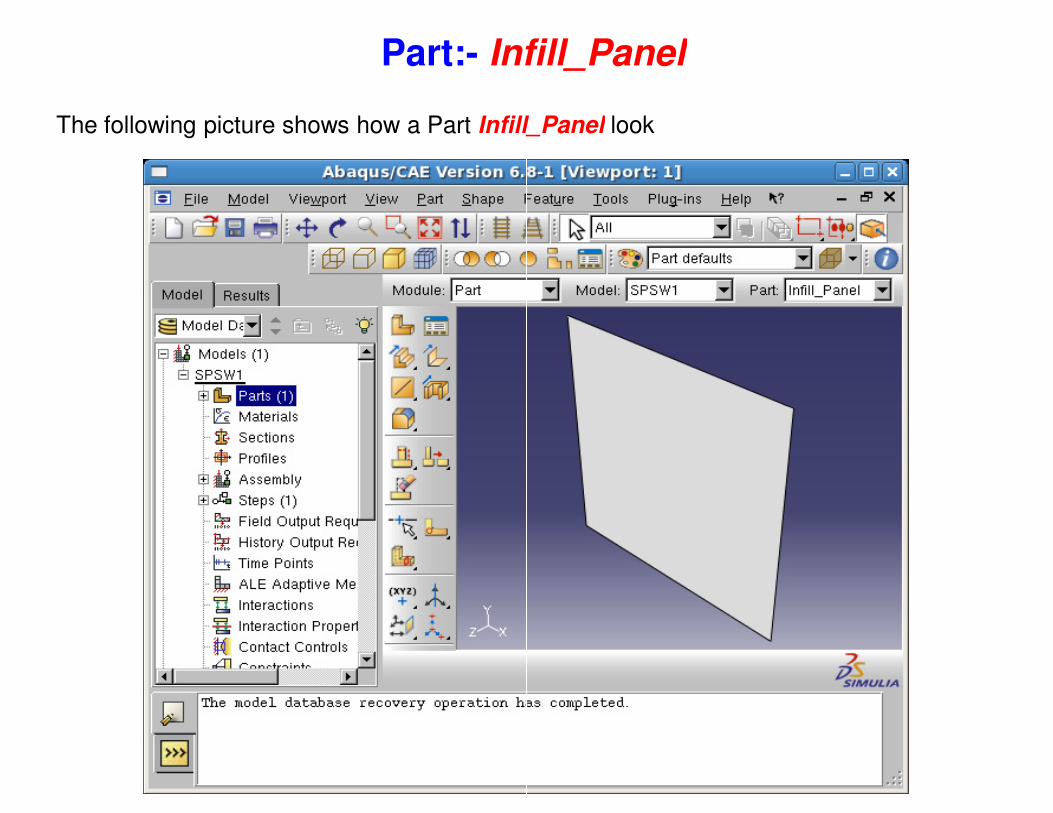
Part:- Infill_Panel
The following picture shows how a Part Infill_Panel
Infill_Panel
Infill_Panel look
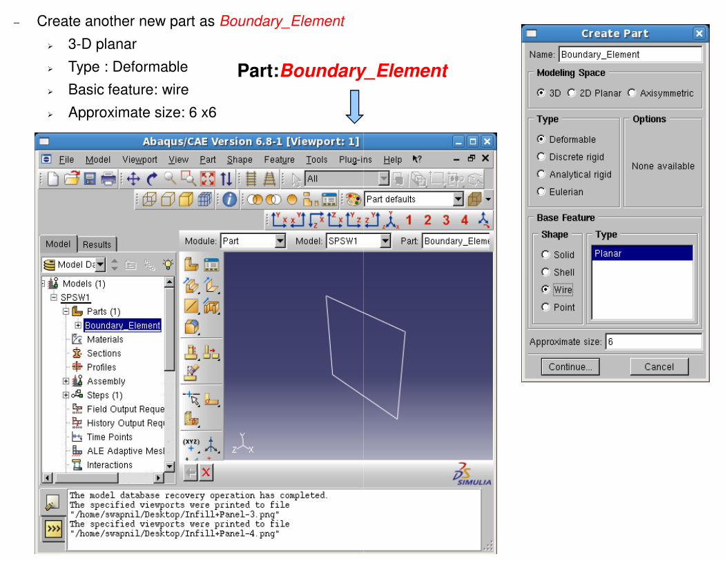
− Create another new part as Boundary_Element
� 3-D planar
� Type : Deformable
� Basic feature: wire
� Approximate size: 6 x6
Part:Boundary_ElementBoundary_Element
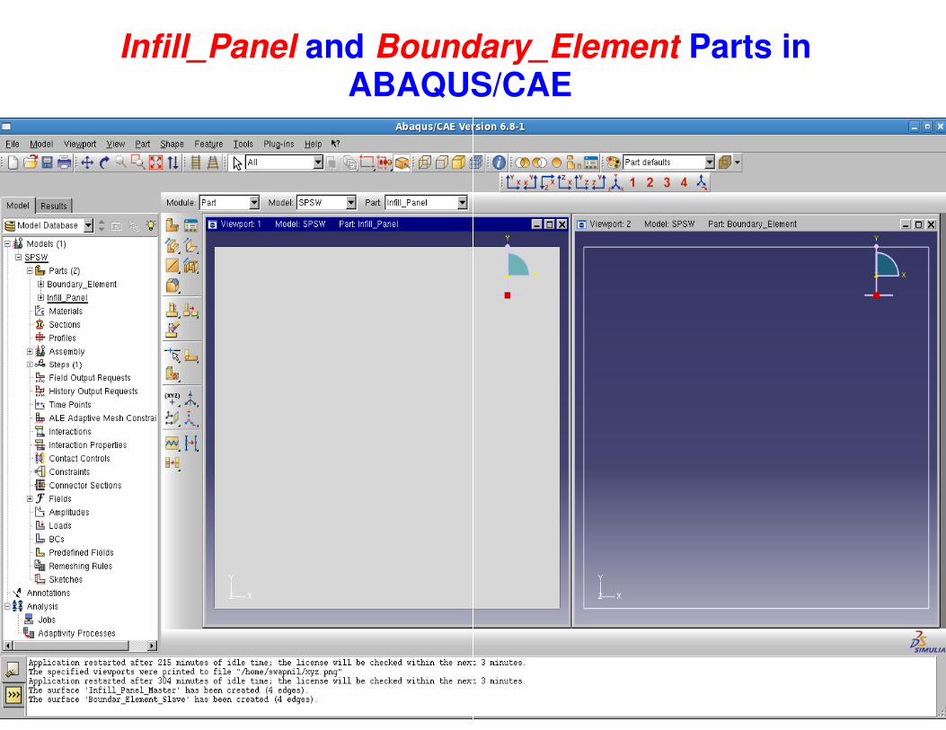
Infill_Panel and Boundary_ElementABAQUS/CAE
Boundary_Element Parts in ABAQUS/CAE
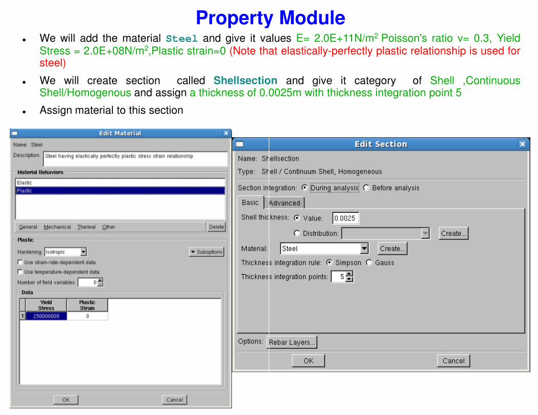
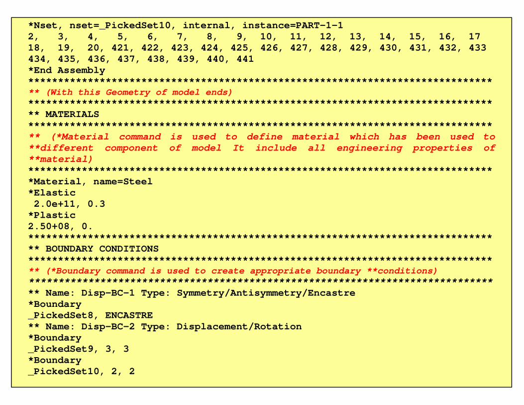
� We will add the material Steel and give it valuesStress = 2.0E+08N/m2,Plastic strain=0 (Note thatsteel)
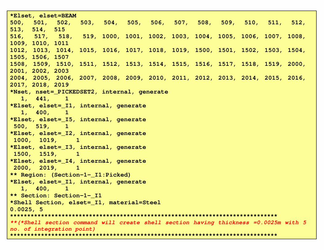
� We will create section called ShellsectionShell/Homogenous and assign a thickness of 0.0025
� Assign material to this section
Property Modulevalues E= 2.0E+11N/m2 Poisson's ratio ν= 0.3, Yieldthat elastically-perfectly plastic relationship is used for
Shellsection and give it category of Shell ,Continuous0025m with thickness integration point 5
Property Module
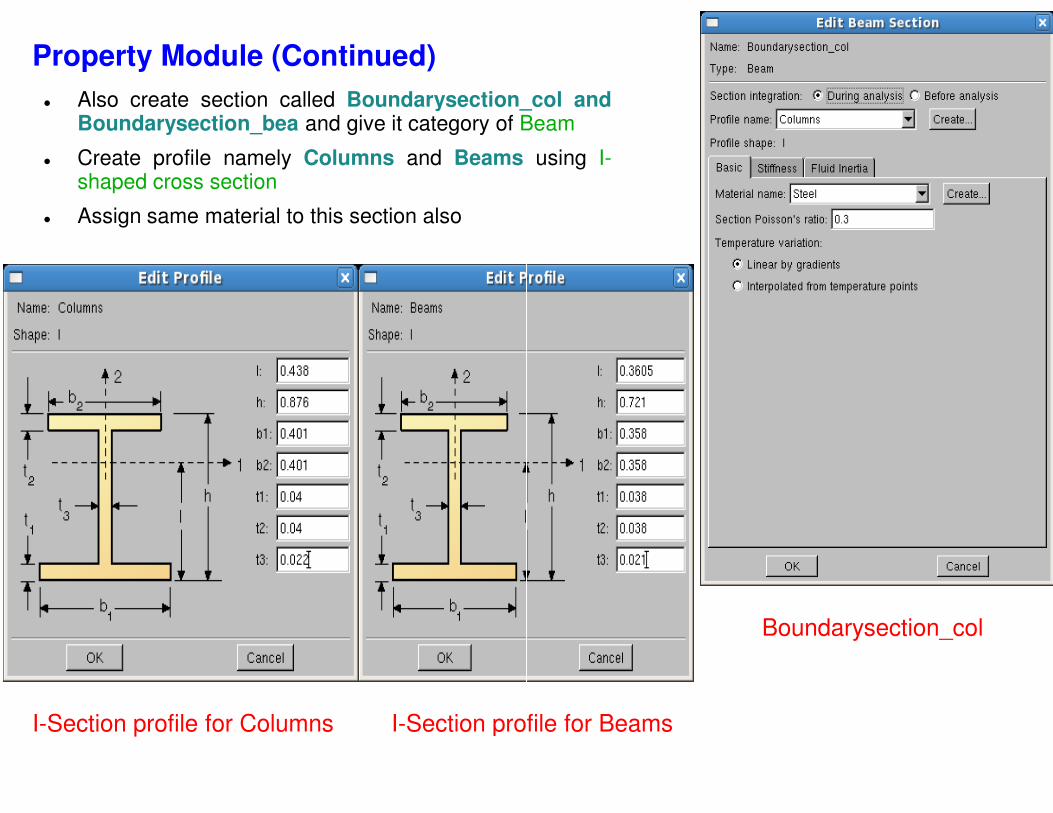
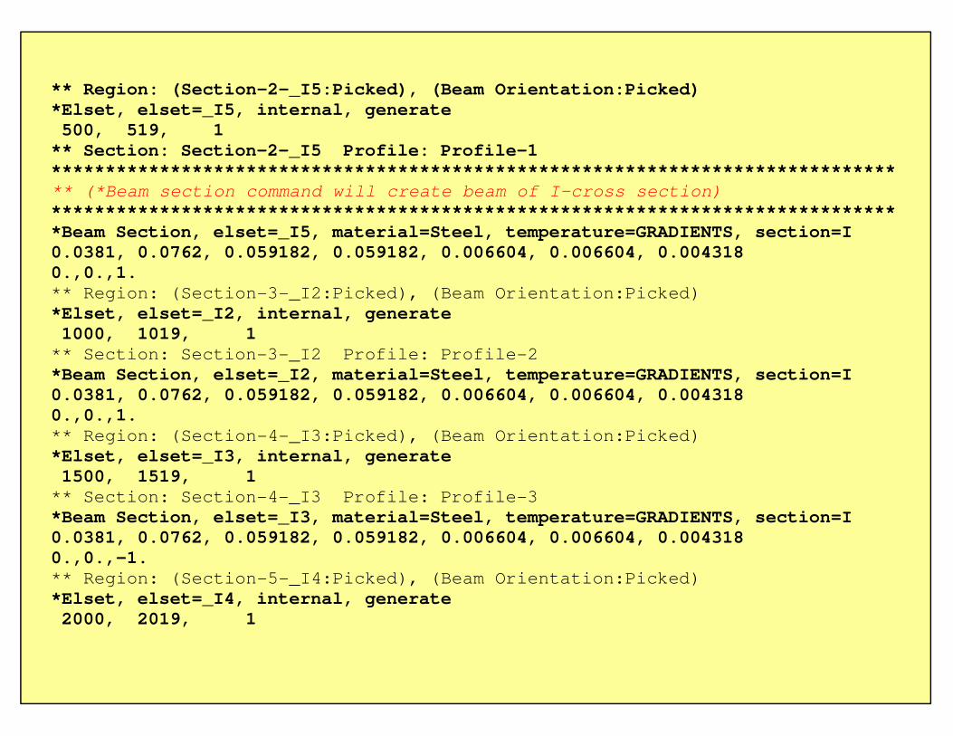
� Also create section called Boundarysection_colBoundarysection_bea and give it category of Beam
� Create profile namely Columns and Beamsshaped cross section
� Assign same material to this section also
Property Module (Continued)
I-Section profile for Columns I-Section profile for Beams
Boundarysection_col andBeam
using I-
Section profile for Beams
Boundarysection_col
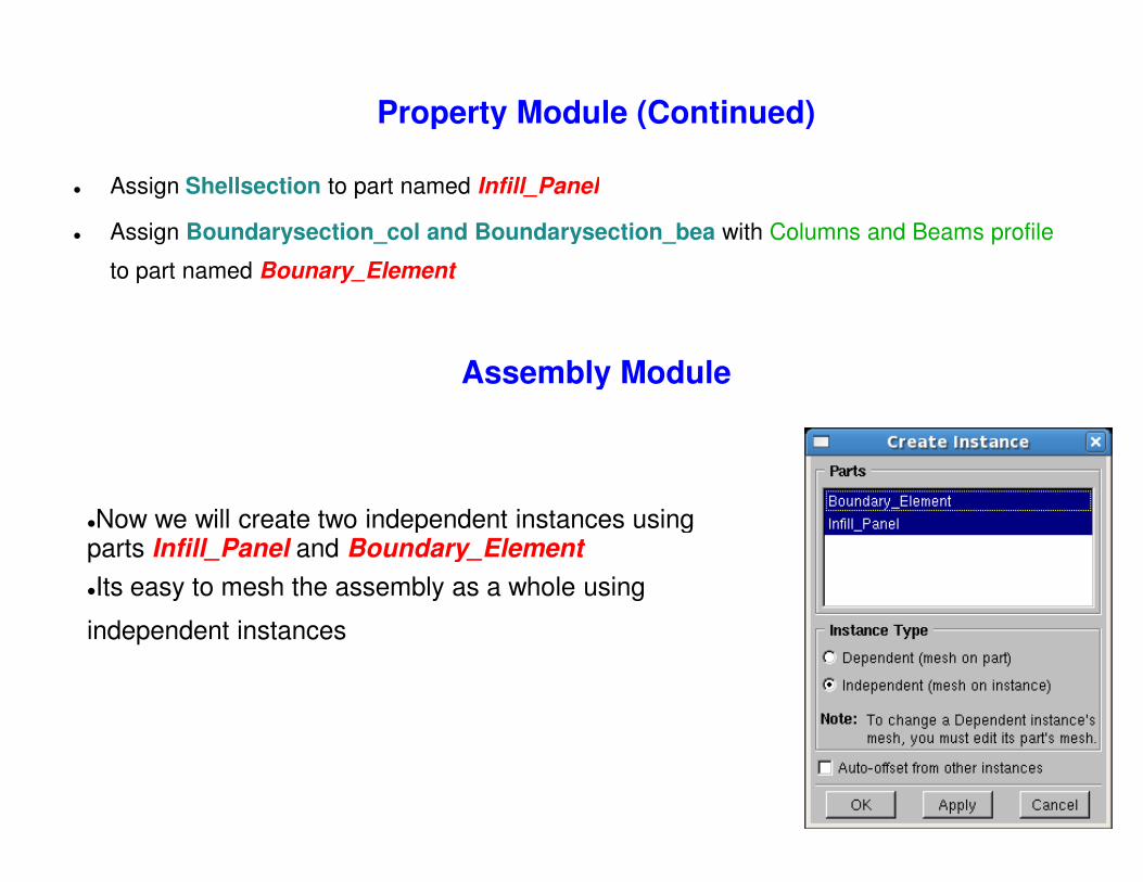
� Assign Shellsection to part named Infill_Panel
� Assign Boundarysection_col and Boundarysection_bea
to part named Bounary_Element
Property Module (Continued)
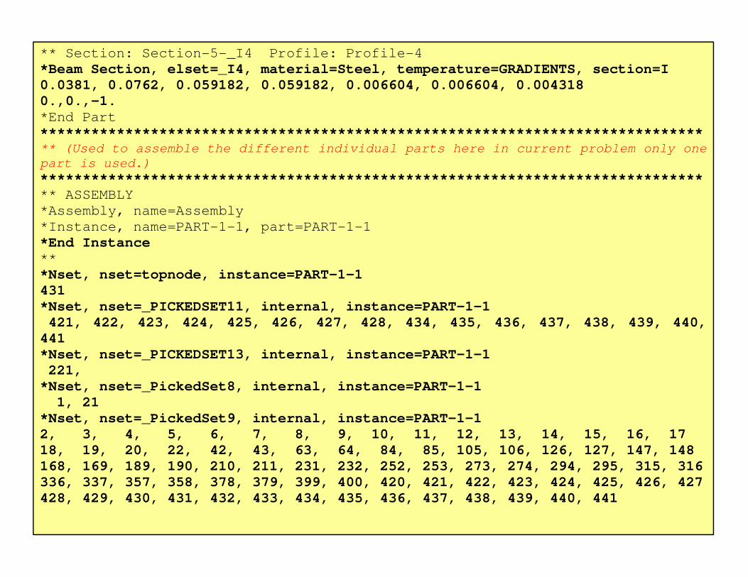
Assembly Module
�Now we will create two independent instances using parts Infill_Panel and Boundary_Element
�Its easy to mesh the assembly as a whole using
independent instances
Infill_Panel
Boundarysection_bea with Columns and Beams profile
Property Module (Continued)
Assembly Module
Now we will create two independent instances using Boundary_Element
Its easy to mesh the assembly as a whole using
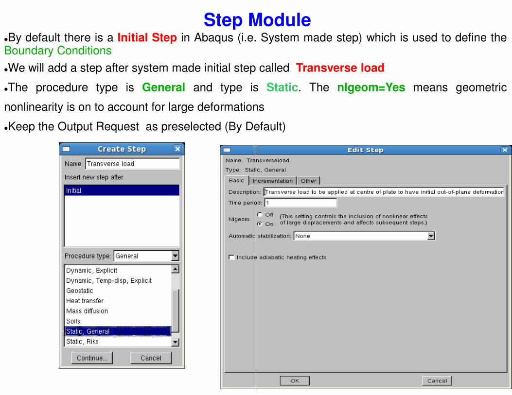
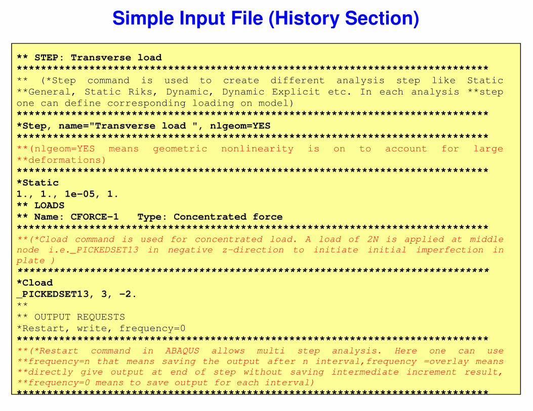
Step Module�By default there is a Initial Step in Abaqus (i.e.Boundary Conditions
�We will add a step after system made initial step
�The procedure type is General and type is
nonlinearity is on to account for large deformations
�Keep the Output Request as preselected (By Default)
Step Module. System made step) which is used to define the
called Transverse load
is Static. The nlgeom=Yes means geometric
deformations
Default)
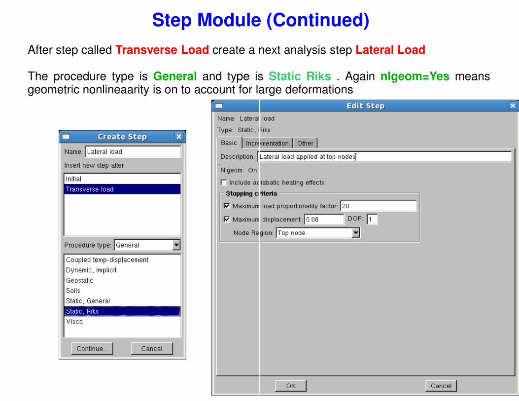
Step Module (Continued)
After step called Transverse Load create a next
The procedure type is General and type isgeometric nonlineaarity is on to account for large
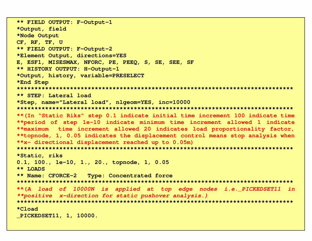
Step Module (Continued)
next analysis step Lateral Load
is Static Riks . Again nlgeom=Yes meanslarge deformations
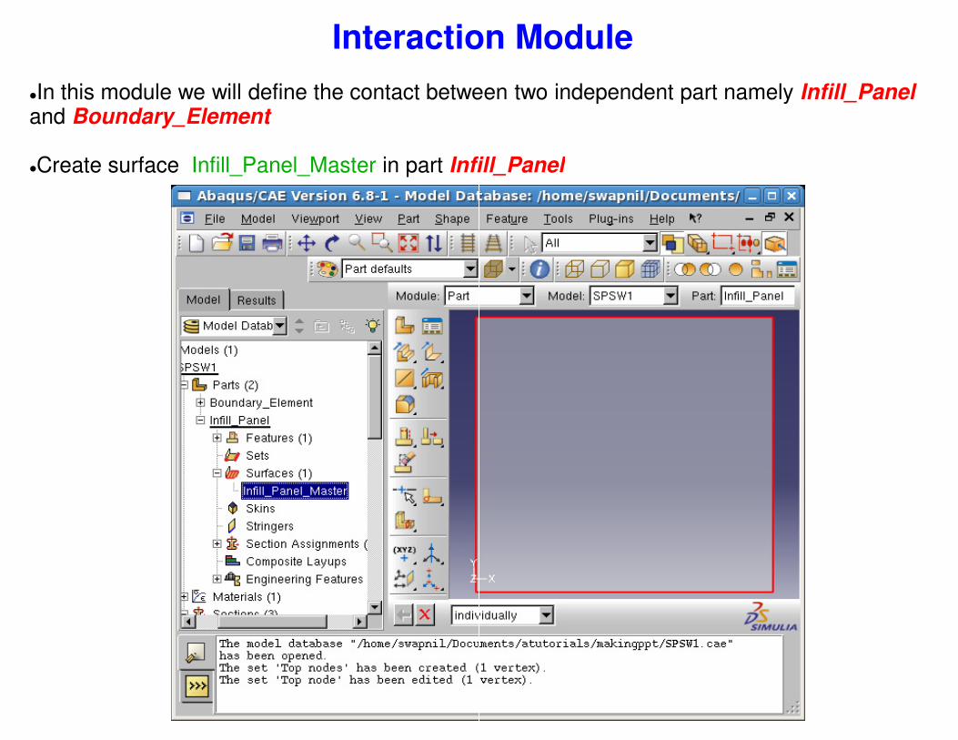
Interaction Module
�In this module we will define the contact between two independent part namelyand Boundary_Element
�Create surface Infill_Panel_Master in part Infill_Panel
Interaction Module
In this module we will define the contact between two independent part namely Infill_Panel
Infill_Panel
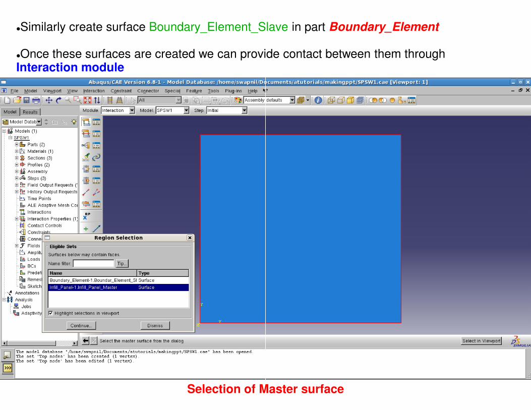
�Similarly create surface Boundary_Element_Slave
�Once these surfaces are created we can provide contact between them through Interaction module
Selection of Master surface
Boundary_Element_Slave in part Boundary_Element
Once these surfaces are created we can provide contact between them through
Selection of Master surface
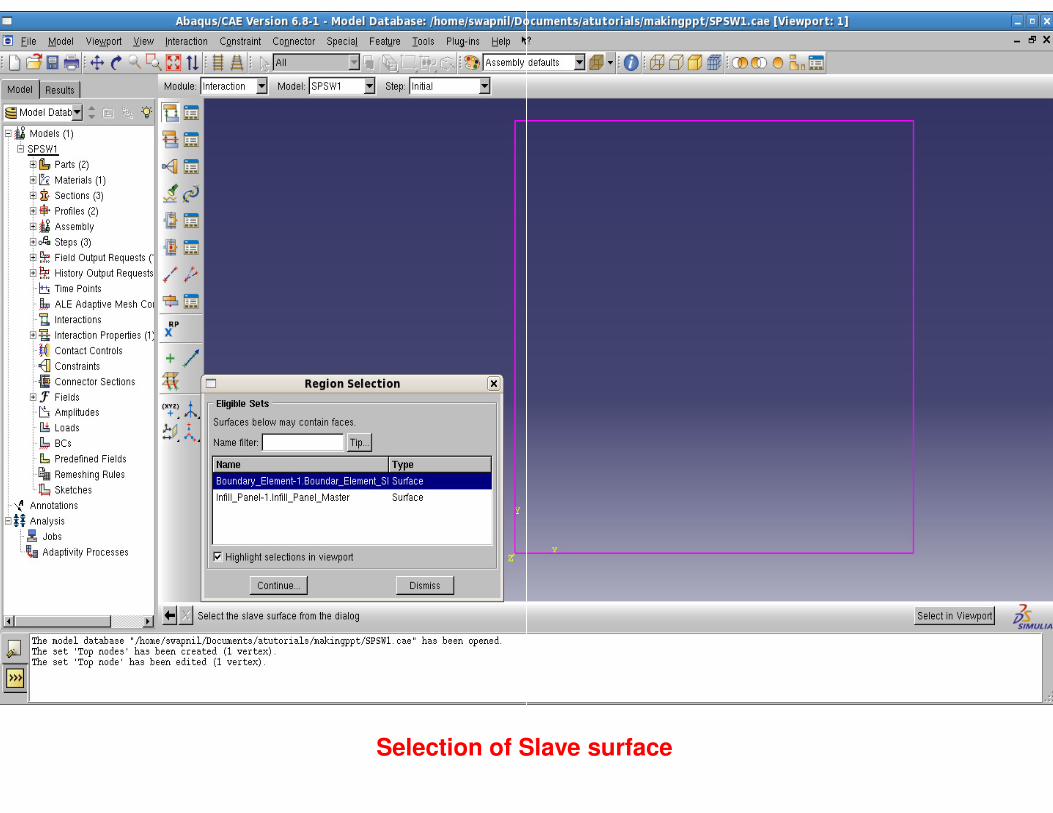
Selection of Slave surfaceSelection of Slave surface
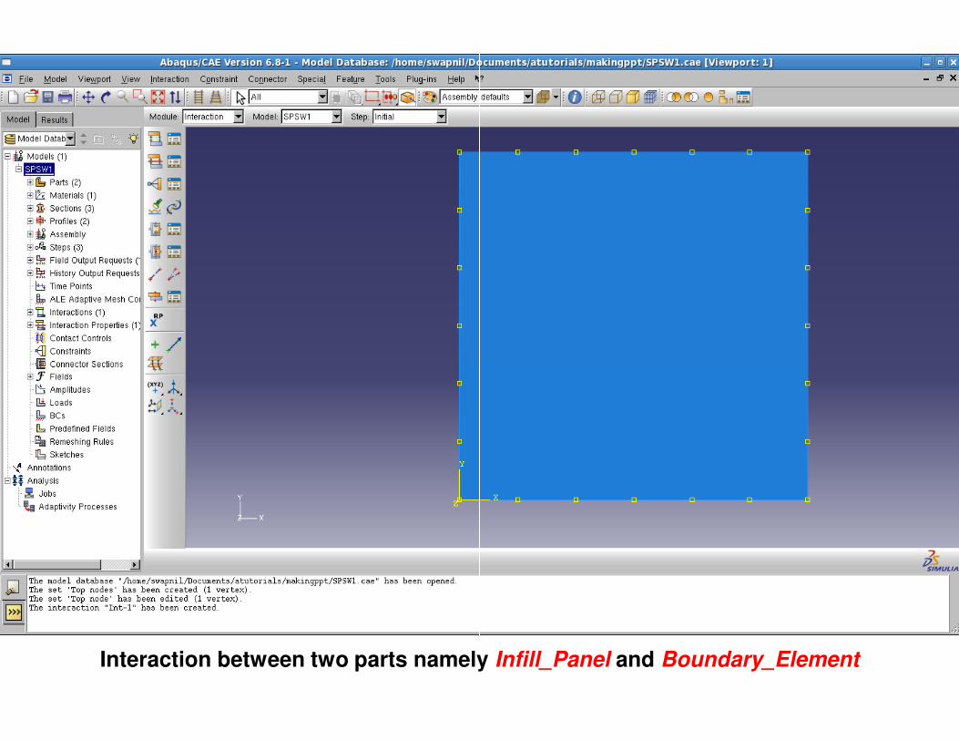
Interaction between two parts namelyInteraction between two parts namely Infill_Panel and Boundary_Element
Creating Boundary Conditions in Initial Step
�Create boundary conditions in Initial step (System made step)
�There are two type of Boundary conditions for this problem namely
�Bottom extreme nodes are fixed (U1=U2=U3
�Edges are restrained in z-direction (U3=0)
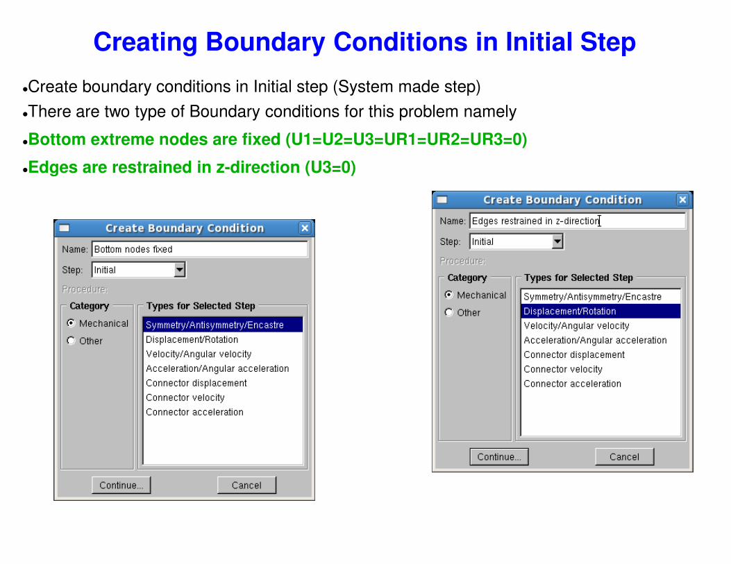
Creating Boundary Conditions in Initial Step
Create boundary conditions in Initial step (System made step)
There are two type of Boundary conditions for this problem namely
3=UR1=UR2=UR3=0)
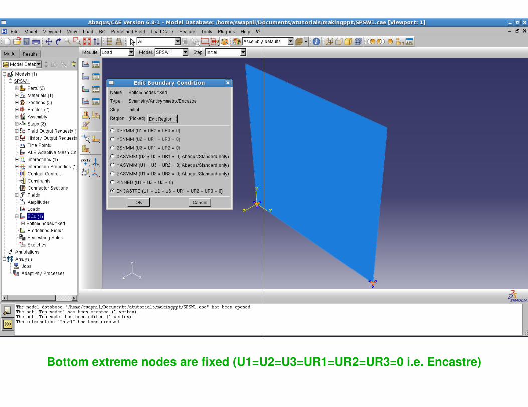
Bottom extreme nodes are fixed (U1=U=U2=U3=UR1=UR2=UR3=0 i.e. Encastre)
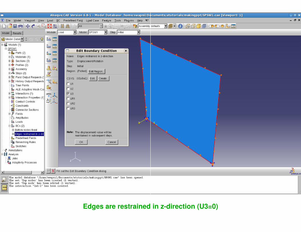
Edges are restrained in zEdges are restrained in z-direction (U3=0)
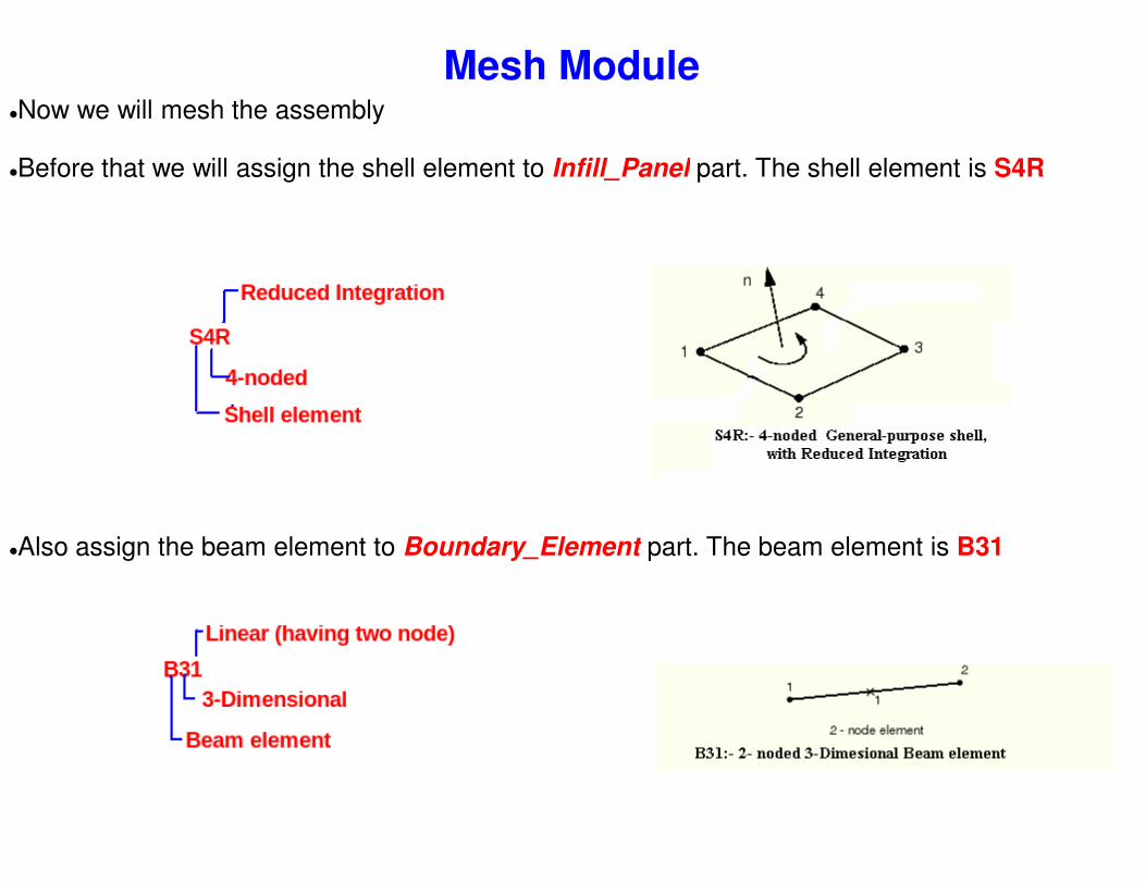
Mesh Module�Now we will mesh the assembly
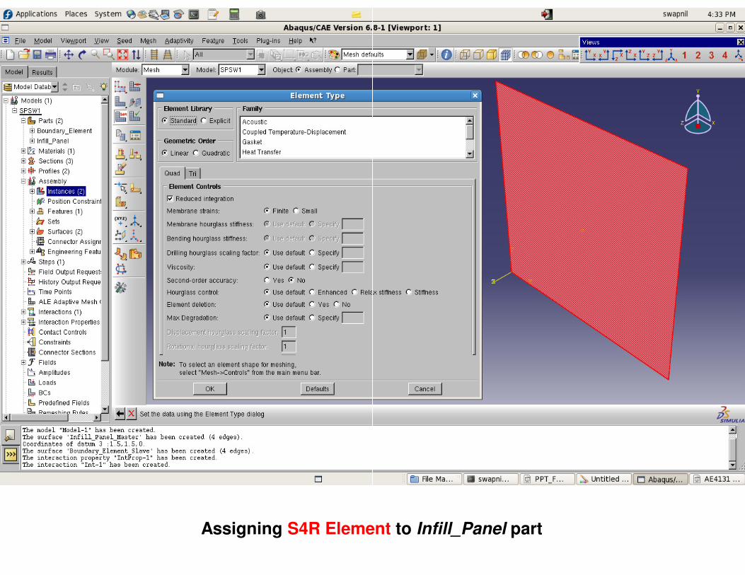
�Before that we will assign the shell element to Infill_Panel
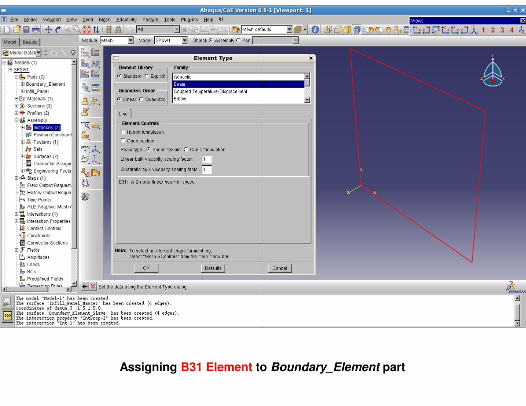
�Also assign the beam element to Boundary_Element
Mesh Module
Infill_Panel part. The shell element is S4R
Boundary_Element part. The beam element is B31
Assigning S4R Element R Element to Infill_Panel part
Assigning B31 Element toto Boundary_Element part
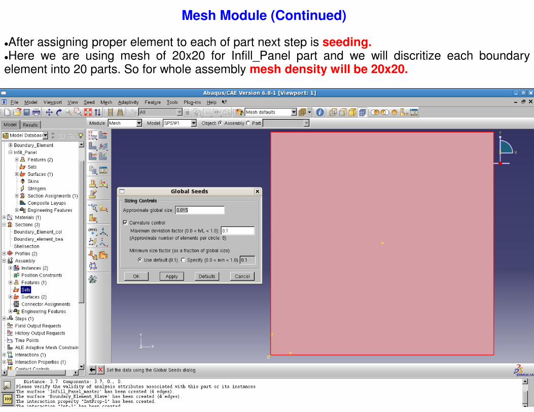
Mesh Module (Continued)
�After assigning proper element to each of part next�Here we are using mesh of 20x20 for Infill_Panelelement into 20 parts. So for whole assembly mesh
Mesh Module (Continued)
next step is seeding.Infill_Panel part and we will discritize each boundary
mesh density will be 20x20.
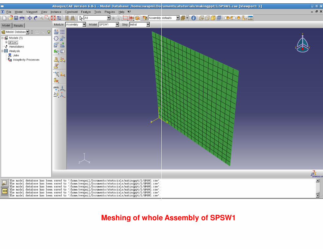
Meshing of whole Assembly of SPSWMeshing of whole Assembly of SPSW1
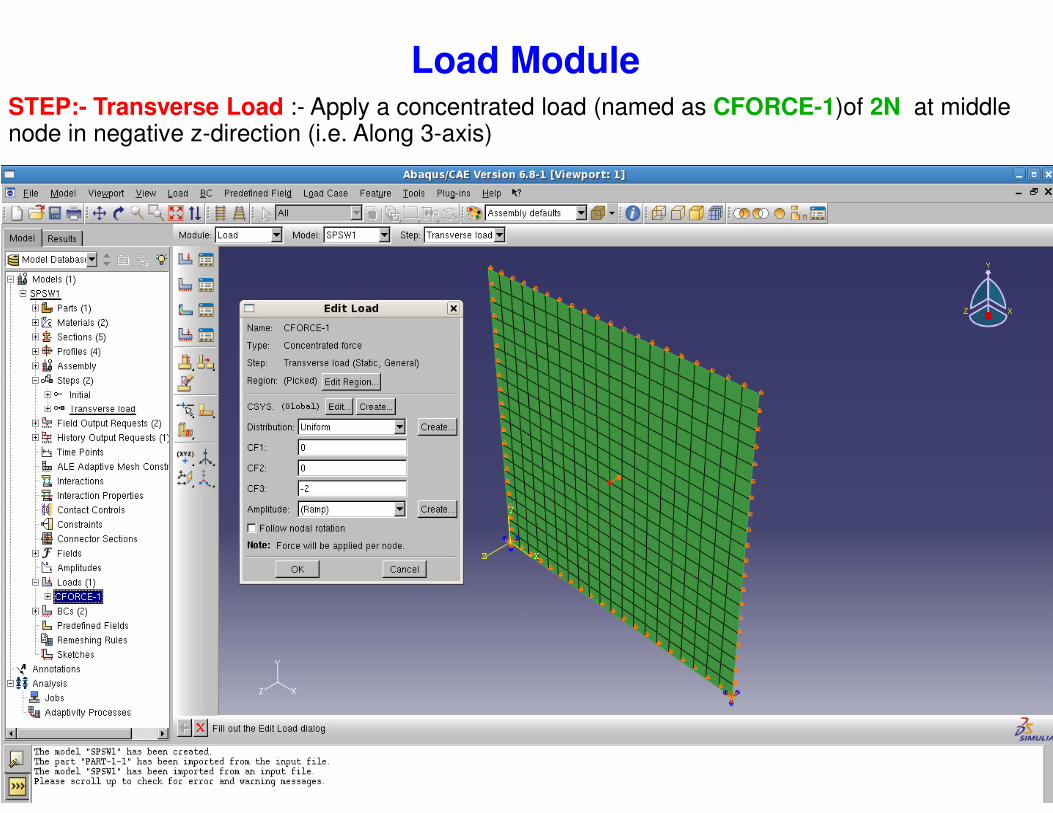
Load Module STEP:- Transverse Load :- Apply a concentrated load (named as node in negative z-direction (i.e. Along 3-axis)
Load Module Apply a concentrated load (named as CFORCE-1)of 2N at middle
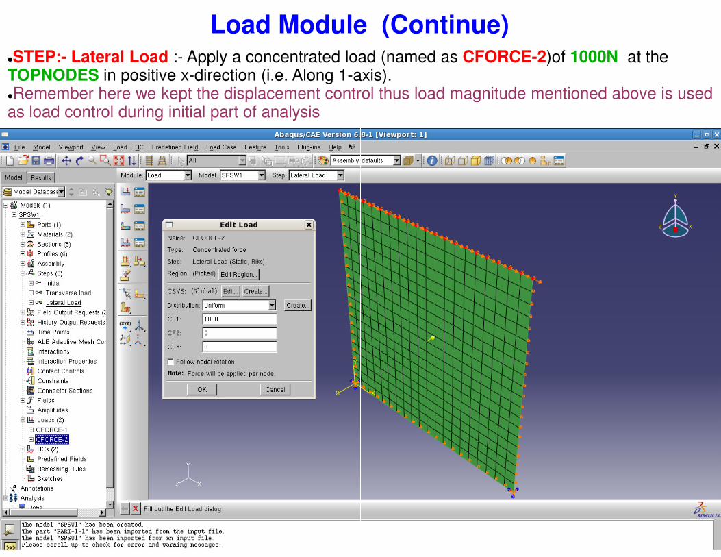
Load Module (Continue)�STEP:- Lateral Load :- Apply a concentrated load (named as TOPNODES in positive x-direction (i.e. Along 1-axis). �Remember here we kept the displacement controas load control during initial part of analysis
Load Module (Continue) Apply a concentrated load (named as CFORCE-2)of 1000N at the
axis). trol thus load magnitude mentioned above is used
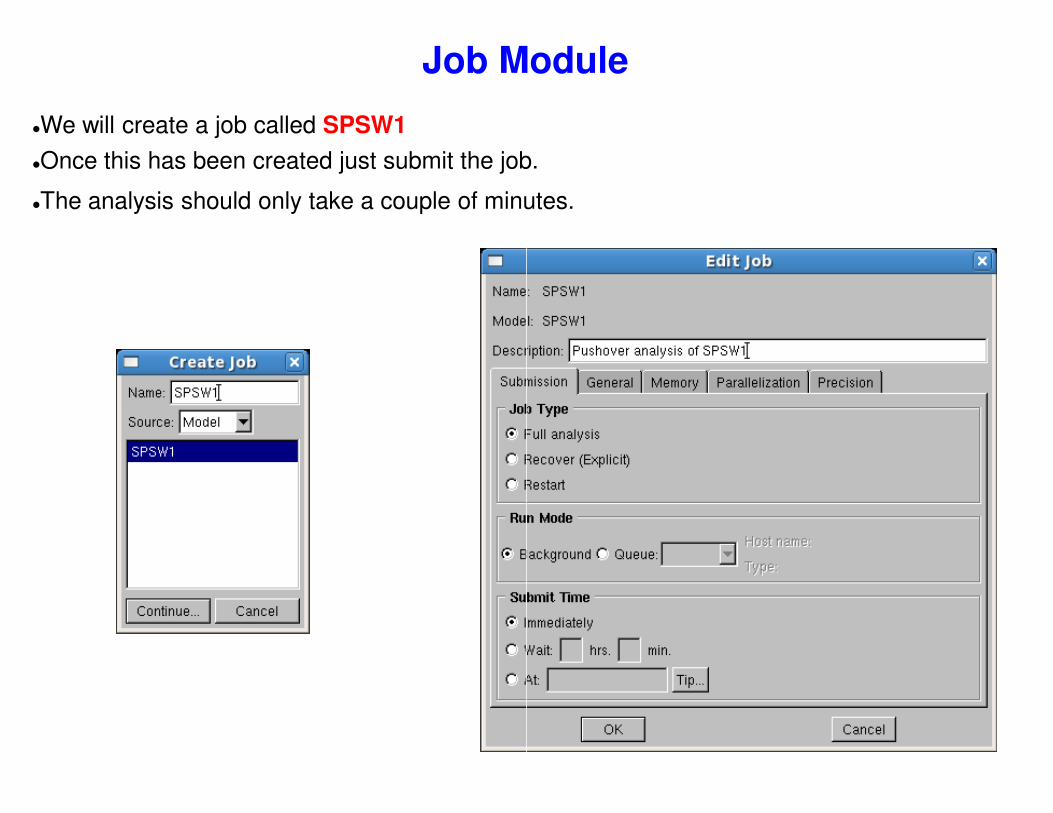
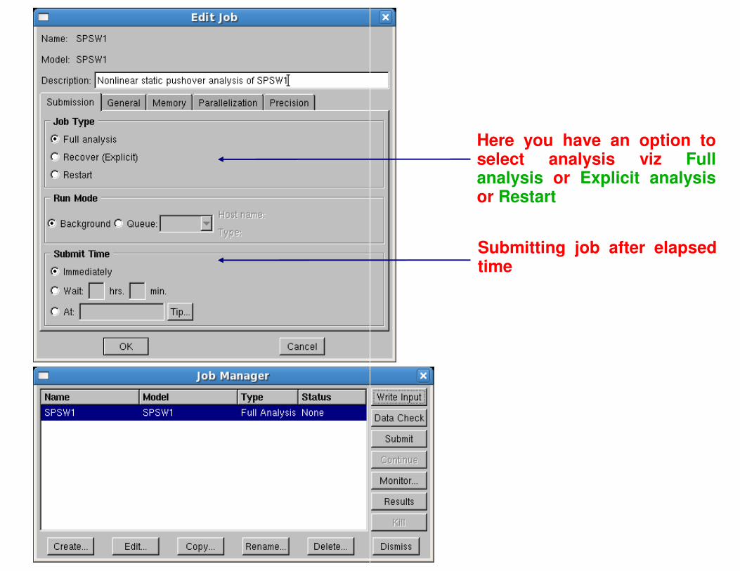
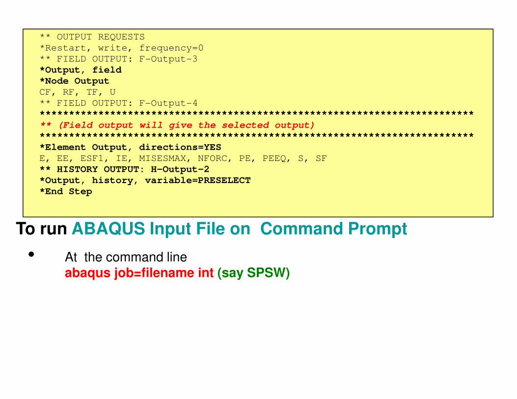
Job Module
�We will create a job called SPSW1
�Once this has been created just submit the job.
�The analysis should only take a couple of minutes.
Job Module
Once this has been created just submit the job.
The analysis should only take a couple of minutes.
Here you have an option toselect analysis viz Fullanalysis or Explicit analysisor Restart
Submitting job after elapsedtime
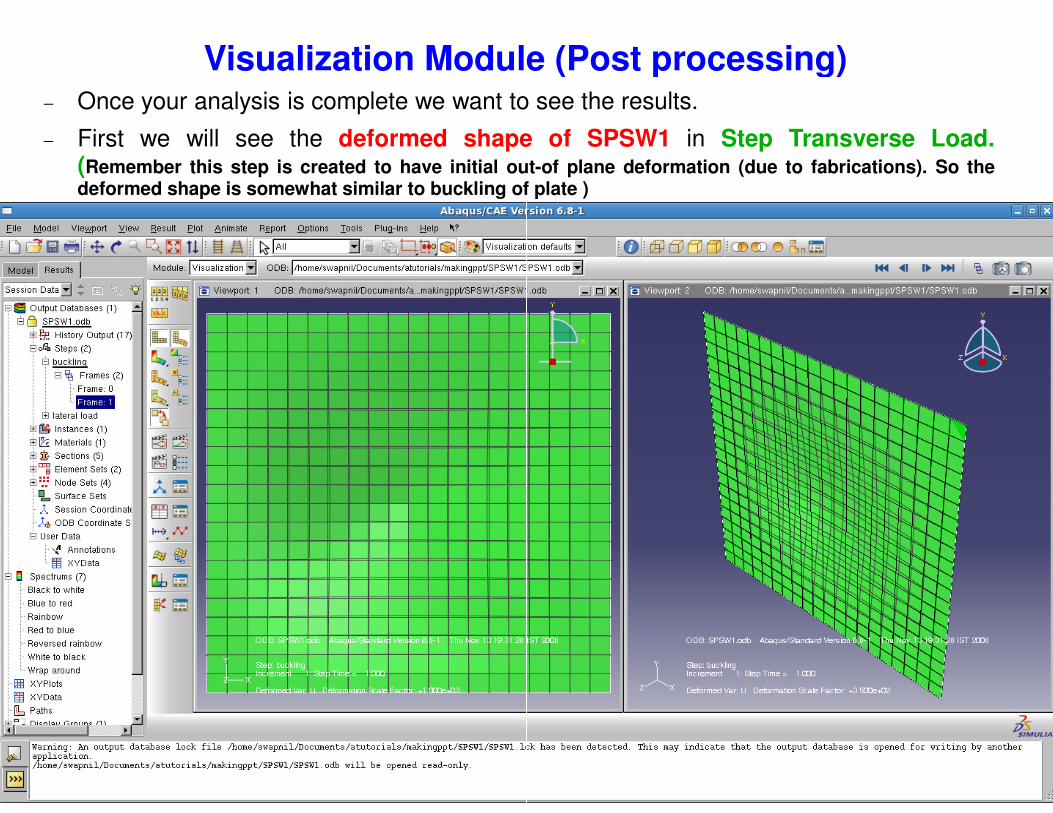
Visualization Module (Post processing)− Once your analysis is complete we want to
− First we will see the deformed shape(Remember this step is created to have initial outdeformed shape is somewhat similar to buckling of
Visualization Module (Post processing) to see the results.
shape of SPSW1 in Step Transverse Load.out-of plane deformation (due to fabrications). So theof plate )
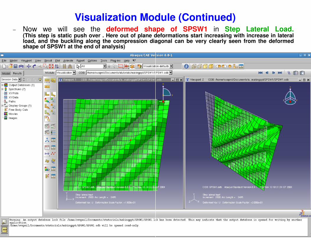
− Now we will see the deformed shape(This step is static push over . Here out of plane deformationsload, and the buckling along the compression diagonalshape of SPSW1 at the end of analysis)
Visualization Module (Continued)shape of SPSW1 in Step Lateral Load.
deformations start increasing with increase in lateraldiagonal can be very clearly seen from the deformed
Visualization Module (Continued)
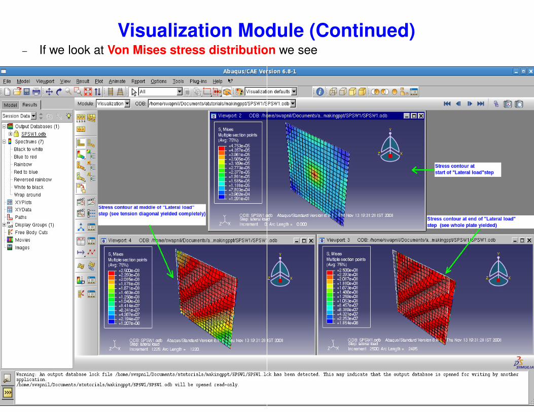
Visualization Module (Continued)− If we look at Von Mises stress distribution
Visualization Module (Continued) stress distribution we see
Visualization Module (Continued)
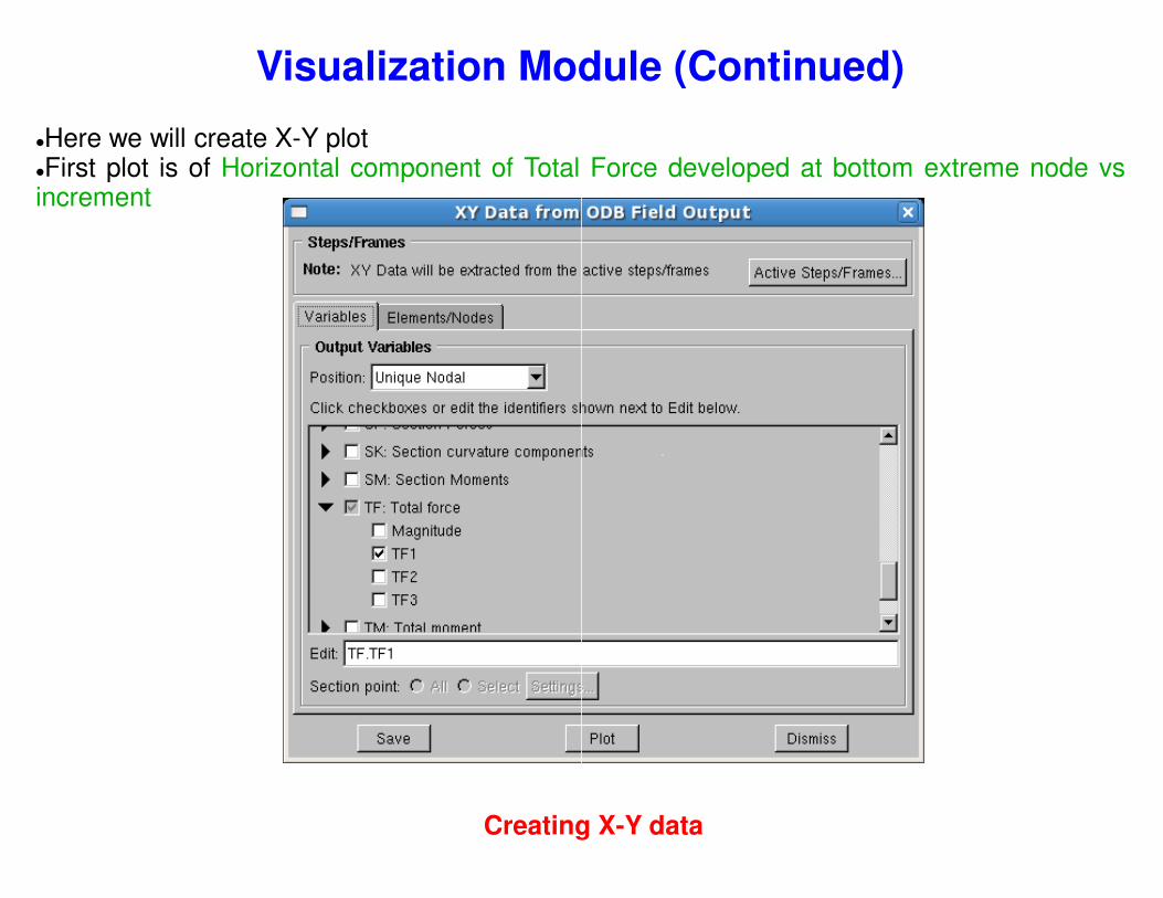
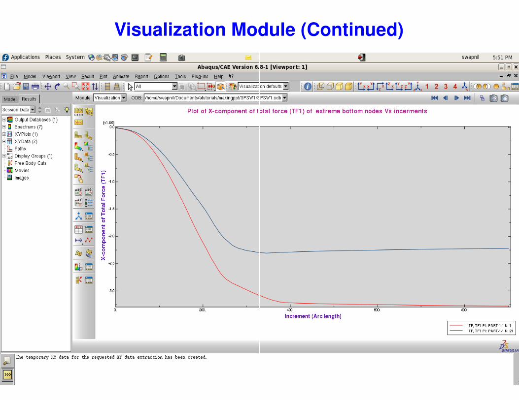
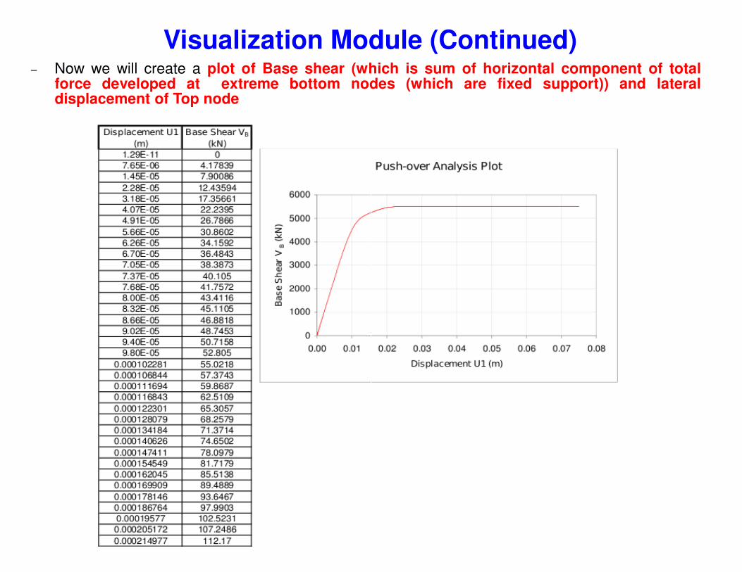
�Here we will create X-Y plot�First plot is of Horizontal component of Totalincrement
Creating X
Visualization Module (Continued)
Force developed at bottom extreme node vs
Creating X-Y data
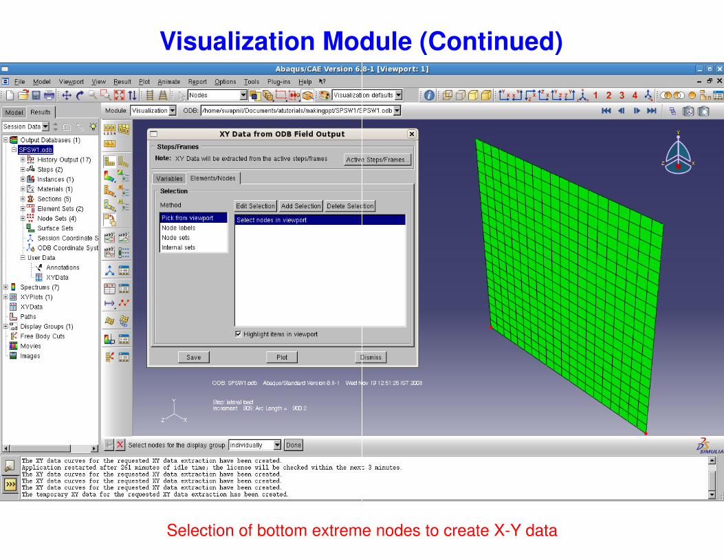
Visualization Module (Continued)
Selection of bottom extreme nodes to create X
Visualization Module (Continued)
Selection of bottom extreme nodes to create X-Y data
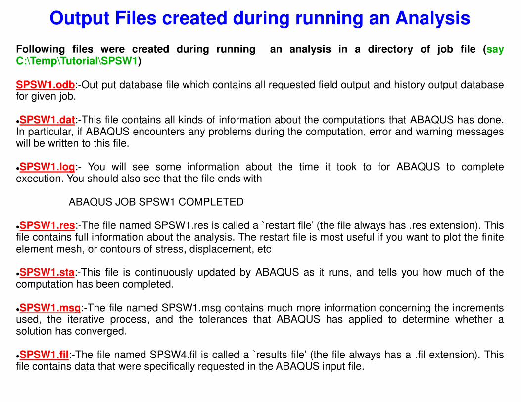
�SPSW1.res:-The file named SPSW1.res is called afile contains full information about the analysis. The restartelement mesh, or contours of stress, displacement, etc
�SPSW1.sta:-This file is continuously updated by ABAQUScomputation has been completed.
�SPSW1.msg:-The file named SPSW1.msg containsused, the iterative process, and the tolerances thatsolution has converged.
�SPSW1.fil:-The file named SPSW4.fil is called a `resultsfile contains data that were specifically requested in the
Output Files created during running an Analysis
an analysis in a directory of job file (say
all requested field output and history output database
information about the computations that ABAQUS has done.during the computation, error and warning messages
about the time it took to for ABAQUS to completewith
`restart file’ (the file always has .res extension). Thisrestart file is most useful if you want to plot the finiteetc
ABAQUS as it runs, and tells you how much of the
contains much more information concerning the incrementsthat ABAQUS has applied to determine whether a
`results file’ (the file always has a .fil extension). Thisthe ABAQUS input file.


![Swapnil Project[1]](https://static.documents.pub/doc/80x56/577d29561a28ab4e1ea681ea/swapnil-project1.jpg)


