84
Chapter 20, Seismic Hazard Analysis 2014 DRAFT FERC Engineering Guidelines Risk-Informed Decision Making Chapter R20 Probabilistic Seismic Hazard Analysis

Chapter 20, Seismic Hazard Analysis 2014 DRAFT
FERC Engineering Guidelines
Risk-Informed Decision Making
Chapter R20
Probabilistic Seismic Hazard Analysis

Chapter 20, Seismic Hazard Analysis 2014 DRAFT
Table of Contents Chapter R20 – Probabilistic Seismic Hazard Analysis .................................................. - 1 -
R20.1 Purpose .............................................................................................................. - 1 -
R20.2 Introduction ....................................................................................................... - 2 -
R20.2.1 General Concepts ....................................................................................... - 2 -
R20.2.2 Probabilistic vs. Deterministic Approach .................................................. - 2 -
R20.2.3 Consistency of Seismic Loading Criteria ...... Error! Bookmark not defined.
R20.2.4 PSHA Process ............................................................................................ - 3 -
R20.2.5 Response Spectra Used for Fragility Analysis ........................................... - 4 -
R20.2.6 Selecting Appropriate Seismic Loading..................................................... - 5 -
R20.3 PSHA Data Requirements ................................................................................. - 5 -
R20.3.1 PSHA Inputs ............................................................................................... - 5 -
R20.3.2 General Guide on PSHA Data Collection .................................................. - 6 -
R20.4 Seismic Source Identification ........................................................................... - 7 -
R20.4.1 Type of Faulting ......................................................................................... - 8 -
R20.4.2 Fault Rupture .............................................................................................. - 9 -
R20.4.3 Key Fault Parameters ................................................................................. - 9 -
R20.4.4 Other Seismic Sources ............................................................................. - 10 -
R20.5 Earthquake Magnitude .................................................................................... - 10 -
R20.6 Earthquake Recurrence ................................................................................... - 11 -
R20.7 Source-To-Site Distances ................................................................................ - 15 -
R20.8 Ground Motion Calculation ............................................................................ - 15 -
R20.9 Probabilistic Seismic Hazard Curve ............................................................... - 16 -
R20.9.1 Procedure for Developing the Seismic Hazard Curve ............................. - 18 -
R20.9.2 Computational Tools for PSHA ............................................................... - 20 -
R20.9.3 Comparison with the USGS National Hazard Maps ................................ - 24 -
R20.9.4 Uncertainties in PSHA ............................................................................. - 24 -

Chapter 20, Seismic Hazard Analysis 2014 DRAFT
R20.10 Presentation and Interpretation of PSHA Results ....................................... - 26 -
R20.10.1 Seismic Hazard Curves ......................................................................... - 27 -
R20.10.2 Deaggregation ....................................................................................... - 27 -
R20.10.3 Uniform Hazard Spectra ....................................................................... - 28 -
R20.10.4 Realistic Scenario Earthquake Spectra ................................................. - 29 -
R20.10.5 Conditional Mean Spectra .................................................................... - 29 -
R20.10.6 Median Spectra ..................................................................................... - 32 -
R20.10.7 Time Histories ....................................................................................... - 32 -
R20.11 Senior Seismic Hazard Analysis Committee (SSHAC) Guidelines ............ - 33 -
R20.12 Using PSHA Curves .................................................................................... - 38 -
R20.12.1 Fragility Analyses ................................................................................ - 38 -
R20.12.2 Simplified Method for PSHA ............................................................... - 39 -
R20.13 RIDM Seismic Methodology....................................................................... - 41 -
REFERENCES ............................................................................................................... - 1 -

Chapter 20, Seismic Hazard Analysis - 1 - 2014 DRAFT
Chapter R20 – Probabilistic Seismic Hazard Analysis
R20.1 Purpose
The purpose of this chapter is to provide guidance for developing probabilistic seismic hazard curves for use in the safety evaluation of FERC-regulated hydroelectric facilities. The guidelines fit within the framework of risk-informed decision making (RIDM) process described by other FERC RIDM Engineering Guidelines (EGs). The seismic risk estimate is calculated by integrating the seismic hazard curves derived from Probabilistic Seismic Hazard Analysis (PSHA) with fragility (probability of failure) of the dam and the consequence of dam failure. The chapter describes how to calculate the seismic ground motions as a function of the return period or annual probability of exceedance and use the results in the estimate of seismic risk. Specifically, this chapter describes how to:
1) Develop probabilities of seismic sources and the earthquake recurrence interval based on the historic and geologic (slip rate) information,
2) Develop probabilistic ground motions, 3) Develop seismic hazard curves using these analyses, 4) Incorporate the “conditional mean spectrum” as a tool for selecting ground
motions as input to dynamic analysis, 5) Use the SSHAC guidance document, as appropriate, to calculate the
uncertainties in PSHA curves and use expert judgment in evaluating uncertainty,
6) Develop a scalable set of levels of seismic hazard evaluation from published probability maps through the highest level of evaluation using expert elicitation and structured expert interaction (described in Chapter R24 of the RIDM EGs),
7) Incorporate the Federal Risk Best Practices in dam seismic hazard evaluation, as applicable, and
8) Show examples of seismic hazard analysis for dams.

Chapter 20, Seismic Hazard Analysis - 2 - 2014 DRAFT
R20.2 Introduction
R20.2.1 General Concepts This section introduces the concepts of seismic hazard analysis and discusses uncertainties associated with hazard analysis and some of the related issues and concerns commonly encountered in practice.
R20.2.2 Probabilistic vs. Deterministic Approach Two basic approaches have been used in developing design ground motions: deterministic and probabilistic seismic hazard analyses. The traditional standards-based (deterministic) approach is typically performed by selecting an earthquake scenario that can reasonably be expected to produce the largest seismic demand (ground motion) on the dam, referred to as the Maximum Credible Earthquake (MCE). Developing the MCE involves these general steps: identify the location and characteristics of all significant potential earthquake sources (faults and/or seismic zones); estimate the maximum magnitude on each source and the appropriate distance to the site; and calculate the ground motion parameters using one or more ground motion models (attenuation relationships). The deterministic analysis considers one source, one magnitude and one distance at a time. The ground motion obtained from deterministic method is typically considered independent of time with the earthquake recurrence assumed to be the same for all seismic sources. The PSHA involves an element of time and uses all possible earthquake scenarios and probability levels as inputs to the seismic load for the dam. The probabilistic approach also incorporates the uncertainties in earthquake locations, earthquake size and ground motion models. Furthermore, in a RIDM analysis, the likelihood of dam failure is defined in terms of probabilities rather than factors of safety. The procedure for a probabilistic approach includes the following steps:
1) define the earthquake source seismicity and geometry, 2) estimate the maximum magnitude for each source and earthquake
occurrence rates, 3) calculate the ground motion parameters using one or more ground motion
models appropriate for the seismic sources, seismotectonic setting and site conditions,
4) develop the uncertainty associated with each step 5) develop the seismic hazard curves and uniform hazard spectrum/
conditional mean spectrum

Chapter 20, Seismic Hazard Analysis - 3 - 2014 DRAFT
R20.2.4 PSHA Process The PSHA process generally consists of two key inputs: seismic source characterization and ground motion predictions as depicted in Steps 1 through 3 of Figure 20-1. Quantification of uncertainty is typically incorporated in each step of PSHA process, including distance to site, earthquake magnitude and recurrence interval, and ground motions. After each of the uncertainties is included in a PSHA, the result is a seismic hazard curve that relates the design motion parameter to the probability of exceedance as shown in Step 4.

Chapter 20, Seismic Hazard Analysis - 4 - 2014 DRAFT
Figure 20-1 Four steps in PSHA (modified from Reiter, 1990).
The seismic hazard curve is the outcome from a PSHA. These steps are further described in Sections R20.4.4 through R20.4.8, below.
R20.2.5 Response Spectra Used for Fragility Analysis After completing the PSHA, the ground motions from seed recordings are selected by scaling and matching them to the target response spectrum. Those matched ground motions are then used as input to dynamic analyses to determine the dam’s fragility to seismic loading at different levels of input motions. By coupling ground motion hazard curves with fragility curves, the probabilities of dam failure can be estimated. It should also be pointed out that the probability of a dam failure would depend on the type of structure and potential failure modes being considered (e.g. liquefaction, sliding, deformations, piping, settlement, etc.). That is, an embankment or concrete dam is expected to respond differently at the same level of input motion.
Uncertainty
M6
Area Source
SITE
Point Source
Fault
Magnitude M
Distance
Peak Acceleration
Step 3: Ground Motion Step 4: Seismic Hazard Curve
Prob. of Exceedance
Ground Motion Parameter
M7
M5
Step 1: Sources Log10 N (m) Step 2: Earthquake Recurrence

Chapter 20, Seismic Hazard Analysis - 5 - 2014 DRAFT
R20.2.6 Selecting Appropriate Seismic Loading
All factors influencing the selection of appropriate ground motions are considered, which include the associated potential failure mode(s), the type, dynamic response and fragility of the dam, and the consequences of dam failure. Incorporating these factors means that additional seismic loading information may need to be developed iteratively with the analyses of the dam.
For a fully quantitative analysis, the seismic risk is calculated using the inputs listed above to annualize the probable life loss using an fN or FN chart. This allows for a calculation of “As Low As Reasonably Practicable” (ALARP) for each dam. For more discussion of these concepts see Chapters R24 and R27, Risk Analysis and Risk Assessment.
A simplified seismic risk procedure is discussed in Section R20.12.2. The output from this procedure should only be considered an interim result.
R20.3 PSHA Data Requirements
R20.3.1 PSHA Inputs In order to perform a PSHA, geological, seismological, geophysical, and geotechnical data must be available to establish the characteristics of seismic sources and ground motions at a site. Numerous maps are available that can be consulted as a first step in evaluating whether or not to undertake site-specific studies. The seismic source data generally include:
• geometries (fault source: length, dip, depth; area source: area, depth) • fault type (strike-slip, normal, thrust) • fault activity (slip rates) • fault location • maximum magnitudes • earthquake recurrence interval (Step 2 in Fig. 3-1)
In practice, it is common that an analyst is faced with insufficient data on maximum or characteristic events for defining the likelihood of an earthquake event. The historical seismicity record is generally too short to characterize the recurrence characteristics of particular faults (Youngs and Coppersmith, 1985). In this case, geologic data such as slip rates are used to estimate maximum earthquake magnitudes and the earthquake recurrence interval. Slip rates are also used to show the sensitivity of seismic hazard estimates to fault specific seismicity parameters.

Chapter 20, Seismic Hazard Analysis - 6 - 2014 DRAFT
The most common parameters associated with ground motion predictions (Step 3 in Fig. 3-1) include:
• earthquake scenarios (magnitude and distance) • type of faulting • local site conditions (shear wave velocity, dynamic material properties,
amplification, topography)
An in-depth discussion of geological, seismological, and geophysical inputs needed to complete a PSHA can be found in Chapter 13 of the FERC (deterministic) EGs and is not repeated here.
Information needed for the PSHA is obtained from the following sources of data in the region in which the site is located:
1) the historical seismicity record, 2) the seismographic, or instrumental, record of earthquake activity in the
region, and 3) the geologic history, especially within the past few thousand to several
hundred thousand years.
R20.3.2 General Guide on PSHA Data Collection The table below presents the general guide for PSHA data collection based, in part, on current practice employed by various federal agencies. Factors to be considered include the distance from the site, the nature of the Quarternary tectonic regime, the geological complexity of the site and region, the existence of potential seismic sources, the potential for surface deformations, etc. The dam hazard classification and the risk of a dam potential failure are implicitly considered in the guide.
Table 20-1 PSHA Data Collection Guide
Study Level Scope Distance
(km) Intended
Use Procedures
Risk Screening Regional >100
Level 1 -2 Risk Analysis (RA)*/ Emergency Planning
Literature reviews, study of maps and remote sensing data, ground truth reconnaissance, develop new hazard curves based on existing readily available data
Intermediate Regional,
Site-specific
100 - 15
Part 12D Safety
Limited field studies, develop seismic source characterization models, produce

Chapter 20, Seismic Hazard Analysis - 7 - 2014 DRAFT
Study Level Scope Distance
(km) Intended
Use Procedures
Review/ Level 2-3 RA*
hazard curves, and develop UHS and time histories if needed.
Detailed design
Site-specific < 15
Level 3-4 RA* Seismic Retrofit
Design for new dam
Identify and characterize the seismic and surface deformation potential of any seismogenic source or capable tectonic source causing surface or near-surface displacement. Assess the ground motion characteristics of soils and rocks in the site vicinity within 5 miles Very detailed geological, geophysical, and geotechnical investigations within a radius of 0.5 mile of the site to assess specific soil and rock characteristics Site-specific field studies, fault trenching, geologic mapping and age dating. Detailed source characterization, possible seismic monitoring. Develop hazard curves, UHS, scenario spectrum, and time histories
* See Chapter R24 of the RIDM for a discussion of Levels of Risk Analysis. USGS data is often acceptable for a Level 1 RA.
R20.4 Seismic Source Identification Step 1 of Figure 20-1 illustrates the three possible seismic sources. Seismic sources that are modeled as point source refer to the epicenter of past earthquakes clustered in a relatively small area and far away from the site (e.g. volcanoes, distant short faults etc.) An areal source is for regions where past seismic activity may not correlate with any of the active geological structure or the available data are not adequate to recognize a particular fault system. There are three fundamental elements associated with seismic source characterization:
1) the identification location and geometry of significant sources of earthquakes,
2) the sizes of the earthquakes associated with these sources, including the maximum, and
3) the rate at which they occur.

Chapter 20, Seismic Hazard Analysis - 8 - 2014 DRAFT
All earthquake sources capable of producing of damaging ground motions at a site are identified through various means such as observations of past earthquake locations and geological evidence. For individual faults that are not particularly identifiable in the less seismically active regions of the eastern United States, the earthquake sources may be described by areal regions in which an earthquake may occur anywhere. The source characterization should include a description of the key sources and a map of faults and source zones and the historical seismicity. There should also be a table that clearly shows the fault and source zone parameters used in the PSHA, including alternative models and parameter values with their associated weights. The dates of past earthquakes on specific faults are also required in addition to the frequency of occurrence. The source parameters for the significant faults (generally within about 100 km) are characterized for input into the hazard analyses. Both areal source zones and Gaussian smoothing of the historical seismicity will be used in the PSHA to account for the hazard from background earthquakes.
R20.4.1 Type of Faulting In many parts of the world, significant earthquake activity can be directly associated with specific faults. There are various types of faults, as shown in Figure 20-2.
a. Thrust faulting under b. Normal faulting resulting from horizontal compressive strains extensional strains
c. Strike-slip displacement d. Under thrust faulting in a vertical fault plane subduction zone
Figure 20-2 Schematic illustration of four types of faults.
Over the years, geologists and seismologists have studied the detailed characteristics of faults, and, until recently, designated each as being a potentially active fault or an inactive fault. This designation is based on how recent the fault displacement is, which

Chapter 20, Seismic Hazard Analysis - 9 - 2014 DRAFT
leads to rigid legal definitions of fault activity based on a specified time criterion. Typically, the more critical the facility, the longer the time criterion specified. For example, the US Nuclear Regulatory Commission considers, for nuclear plants, a fault active if it shows evidence of multiple displacements in the past 500,000 years, or evidence of a single displacement in the past 35,000 years. In the past, the Bureau of Reclamation has recommended 100,000 years, and the US Army Corps of Engineers has recommended 35,000 years for dams. Faults that have had displacements within these time spans are considered active and those that have not had displacements are considered inactive. Risk provides a different setting for the decision about fault activity. The FERC does not recommend any particular limit. The decision about what is a credible fault depends on the judgment of the PSHA analyst, the level of certainty about activity, and the level of rigor needed to support a risk decision. For example, a fault with activity within the last 100,000 years might be considered credible, but the activity (slip) rate is very low, leading to a low likelihood of significant loading. Another consideration might be the uncertainty about activity and, for example, an analyst might assume a likelihood of 0.05 (5%) of the fault being active as one part of an event tree. If the decision about activity is critical to a risk assessment, more site investigation of the fault may be needed. Classifying faults as either "active" or "inactive" does not provide sufficient information about the nature of the fault. Instead, geologists and seismologists have recognized that significant differences exist in the degrees of activity of various faults. These differences are manifested by several key fault parameters, which are briefly described below.
R20.4.2 Fault Rupture The probabilistic assessment of surface rupture hazard is briefly discussed in the Federal Best Practices, Chapter 6, Seismic Hazard Analysis, referenced below. Fault rupture extending to the ground surface could cause damage to the dam and its associated structures such as inlet-outlet systems and tunnels. If a fault crosses or is very near the dam, then a design fault offset should be determined following those empirical methods outlined in Wells and Coppersmith (1994) for all types of faulting and Moss and Ross (2011) for reverse faulting. The probabilistic method as applied to the evaluation of fault rupture hazard is discussed in detail in the paper: A Methodology for Probabilistic Fault Displacement Hazard Analysis (PFDHA) by Youngs et al, 2003. The hazard curve for fault offset has been developed by developed by Youngs et al. (2003) for normal faulting following the PSHA methods for ground shaking. The ground motion attenuation function in PSHA was replaced by a fault displacement attenuation function in PFDHA.
R20.4.3 Key Fault Parameters

Chapter 20, Seismic Hazard Analysis - 10 - 2014 DRAFT
The key fault parameters that appear most significant include: rate of strain release, or fault slip rate; amount of fault displacement in each event; length (and area) of fault rupture; earthquake size; and earthquake recurrence interval. As discussed below in Section R20.7, when paleoseismicity data is not available, earthquake recurrence intervals can be calculated directly from slip rates. The slip rates have also been used to show the sensitivity of calculated seismic hazard estimates to various assumptions regarding fault-specific seismicity parameters and earthquake recurrence models (Youngs and Coppersmith, 1985). Further discussion of these factors can be found in Chapter 13 of the FERC (deterministic) Engineering Guidelines (EGs).
R20.4.4 Other Seismic Sources The sources described in the previous sections consist of specific faults or fault zones. In many parts of the world there are no known or suspected faults and hence seismic activity in those parts cannot be associated with any specific fault or fault zone. In these cases, earthquakes are considered to occur in a "seismic zone" extending over an area that is typically identified based on felt area and/or instrumental seismicity during past earthquakes. This approach is usually used in Eastern North America (ENA) and in some places of Western North America (e.g. Intermountain Seismic Zone and Mt. St Helens Seismic Zone.) Even in geologic settings with a number of known faults, an areal source centered on the site is also considered as a possible seismic source. Often this source is assigned to account for instrumental seismicity that cannot be associated with any known (or suspected) fault. Such a seismic source is usually described as a "random" source and is frequently referred to as a Random Crustal or Background Earthquake. Because this type of event is not associated with a known or mapped fault, there is a level of difficulty in estimating an associated magnitude. In most of the western US, the size of event that would probably produce a recognizable surface expression ranges from about M 6.75 and up; therefore, this would indicate the upper limit of Random Crustal events as M 6.5 ± ¼. Random seismic sources have been assigned in many parts of Western North America (WNA) such as Washington, Oregon and California. The distance from the site to such areal seismic sources is usually assigned as a "depth" below the site and typically varies from 5 to 15 km. Data from instrumental seismicity (which would include the depth of each event) are very helpful in assigning this depth.
R20.5 Earthquake Magnitude

Chapter 20, Seismic Hazard Analysis - 11 - 2014 DRAFT
The “maximum magnitude” is often referred to as the largest magnitude that can occur on a fault. In listing the fault and source zone parameters, the term "maximum magnitude" is often used for both the true maximum magnitude and for the mean magnitude from full rupture of a fault. This is a case where an inconsistent use of terminology can cause confusion in many PSHA reports. In either probabilistic or deterministic seismic hazard analyses, a magnitude is estimated for each fault source based on the fault dimension (area or length), or fault displacements (Wells and Coppersmith, 1994). The magnitude given in models by Wells and Coppersmith is the mean magnitude for the given rupture area with the (aleatory) variability described in terms of the standard deviation. The true maximum magnitude is the magnitude at which the magnitude distribution is truncated (Abrahamson, 2000). For source zones, the maximum magnitude is the largest magnitude that can occur in the source zone. If an exponential distribution is used for the magnitudes (e.g. Gutenberg-Richter model), then the maximum magnitude corresponds to the magnitude at which the exponential distribution is truncated. For faults, the dimension of the fault (length or area) is typically used to estimate the mean magnitude for full rupture of the fault. This mean magnitude is better described as the "mean characteristic magnitude" and not as the maximum magnitude because the PSHA will typically consider a range of ranges about this mean magnitude to account for the variability of the magnitude for a given rupture dimension. For example, the widely used Youngs and Coppersmith (1985) model for the magnitude distribution has the characteristic part of the model centered on the mean characteristic magnitude and the maximum magnitude is 0.25 units larger. For more information about earthquake size and maximum magnitude, see Chapter 13 of the FERC (deterministic) EGs.
R20.6 Earthquake Recurrence A key element in a seismic hazard evaluation is estimating recurrence intervals for various magnitude earthquakes. A general equation that describes earthquake recurrence may be expressed as follows:
𝑵(𝒎) = 𝒇(𝒎, 𝒕) [1]
in which N(m), is the number of earthquakes with magnitude greater than or equal to m, and t is time. The simplest form of Eq. [1] that has been used in most applications is the well-known Richter's law of magnitudes (Gutenberg and Richter, 1956; Richter, 1958) which states

Chapter 20, Seismic Hazard Analysis - 12 - 2014 DRAFT
that the occurrence of earthquakes during a given period of time can be approximated by the exponential relationship:
𝑳𝒐𝒈𝟏𝟎�𝑵(𝒎)� = 𝒂 − 𝒃𝒎 [2] in which 10a is the total number of earthquakes with magnitude greater than zero and b is the slope. This equation describes an exponential magnitude distribution and assumes spatial and temporal independence of all earthquakes, i.e., it has the properties of a Poisson Model. The a and b constants from equation 2 are estimated using statistical analysis of historical observations and geological evidence. The a value indicates the overall rate of earthquakes in a region, and b value indicates the relative ratio of small and large magnitudes (typically b values are approximately equal to 1). For engineering applications, the recurrence is limited to a range of magnitudes between mo and mu. The magnitude mo is the smallest magnitude of concern in the specific application; in most cases mo can be limited to magnitude 5 because little or no damage has occurred from earthquakes with magnitudes less than 5. The magnitude mu is the largest magnitude the fault is considered capable of producing; the value of mu depends on the geologic and seismologic considerations discussed in Chapter 13 of the FERC Deterministic EG. The cumulative distribution is then given by:
𝑭𝑴(𝒎) = 𝑷(𝑴 < 𝒎|(𝒎𝟎 ≤ 𝒎 ≤ 𝒎𝒖))
= 𝑵�𝒎𝟎�−𝑵(𝒎)𝑵�𝒎𝟎�−𝑵(𝒎𝒖)
[3] The probability density function is equal to:
𝒇𝒎(𝒎) = 𝒅𝒅𝒎
(𝑭𝑴(𝒎)) [4] In Equations 1 through 4, the letters m or M refer to magnitude; the upper case M denotes a random variable, and the lower case m denotes a specific value of magnitude. When the recurrence relationship is expressed by Richter's law of magnitudes, the following expression is obtained:
𝑵(𝒎) = 𝑨𝟎 �𝟏 − 𝟏−𝟏𝟎−𝒃(𝒎−𝒎𝟎)
𝟏−𝟏𝟎−𝒃(𝒎𝒖−𝒎𝟎)� [5]
The parameter Ao is the number of events for earthquakes with magnitude greater than or equal to mo (i.e., Log10(Ao) = a − bmo).

Chapter 20, Seismic Hazard Analysis - 13 - 2014 DRAFT
Development of Eq. [5] requires knowledge of the parameters Ao, b, and mu, and a selection of mo. The parameter Ao and slope b are based on either the historical seismicity record (including the instrumental record when available) or on geologic data. The slope b, based on regional historical seismicity records, typically ranges from 0.6 to about 1.1. For most faults, the historical seismic record is relatively short and most of the information is for smaller magnitudes (typically less than 6). Thus, for these smaller magnitude earthquakes, a reasonable fit using Richter's relationship can be obtained and values of Ao and b can be calculated. The other form of an earthquake recurrence model is described as the characteristic earthquake distribution. The characteristic earthquake model implies that a typical size of earthquake ruptures repeatedly along a particular segment of the fault (Schwartz and Coppersmith, 1984). Evidence indicates that the characteristic earthquake model is more appropriate for individual faults than the exponential earthquake magnitude distribution (Youngs and Coppersmith, 1985). In some cases where faults have insufficient recurrence interval data, the geologic slip rates are commonly used to estimate maximum earthquake magnitudes on faults and average earthquake recurrence intervals. The steps involved in calculating the earthquake recurrence rate in terms of the slip rate are as follows:
1. Estimate the maximum earthquake magnitude the fault can produce from Wells and Coppersmith empirical relationships such as those shown in Equations 6a and 6b.
2. Calculate the seismic moment (Equation 7). 3. Estimate the moment rate for the fault from fault dimensions and slip rate
(Equation 8). 4. To determine the rate of recurrence of characteristic earthquakes on the fault,
divide the moment rate Ṁo by the seismic moment Mo. Wells and Coppersmith (1994) established the following empirical relationships between the rupture area, surface rupture length and earthquake magnitude:
Mw = 4.07 + 0.98log10RA [6a] Mw = 5.08 +1.16log10SRL [6b]
where Mw is the moment magnitude, RA is the rupture area, and SRL is the surface rupture length. Seismic moment Mo is obtained from an expression of the form:
Log10Mo = aMw + b [7] where a =1.5 and b = 9.1 based on theoretical considerations and empirical observations.

Chapter 20, Seismic Hazard Analysis - 14 - 2014 DRAFT
Seismic moment rate Ṁo describes the rate of energy release in an earthquake and is given by the following expression:
Ṁo = µAS [8]
where µ is the rigidity or shear modulus (usually taken ~3 x 10¹¹ dyne/cm2), A is the rupture area on the fault plane undergoing slip during the earthquake, and S is the slip rate, usually expressed in mm/year. Discrepancies between earthquake recurrence intervals based on historical seismicity and recurrence intervals based on geologic data are common when applied to a specific fault. An example of the recurrence model for the South Central segment of the San Andreas Fault is shown in Figure 20-3.
Magnitude, m
Figure 20-3 Characteristic earthquake recurrence model for south central segment of San Andreas Fault. This is a plot of the number of earthquakes per year with a magnitude greater than or equal to the magnitude plotted on the abscissa. For example, there is one earthquake every 10 years with a magnitude greater than or equal M 5.

Chapter 20, Seismic Hazard Analysis - 15 - 2014 DRAFT
R20.7 Source-To-Site Distances For large, distant earthquakes, the source-to-site distance can be measured with respect to the epicenter, Repi, or the hypocenter, Rhyp. For sites close to the source, distances can be measured directly from the closest point on the fault rupture. The source-to-site distance is usually identified using both the dip and depth of the fault plane and the geometry of the source. In the 2008 Next Generation of Attenuation Models (NGA) project, several distance definitions have been used such as the closest distance to the rupture plane (Rrup), RJB (also referred to as Joyner-Boore distance) the closest horizontal distance to the surface projection of the rupture; Rx the horizontal distance from the top edge of the rupture, measured perpendicular to the fault strike. Both RJB and RX are used to model the attenuation of hanging wall effects. The distance to the fault is defined to be consistent with the specific attenuation relationship used to calculate the ground motion. Based on the 2008 update of the National Seismic Hazard Maps, the ground motions for the Central and Eastern United States were generally calculated from sources that are up to 1,000 km and in the Western U.S to be less than 200 km from crustal sources and less than 1,000 km from subduction sources.
R20.8 Ground Motion Calculation
The attenuation relationships (also referred to as ground motion prediction equations – GMPEs) are derived from empirical procedures using recorded earthquake ground motion data; analytical procedures, and more recently, coupling the results of analytical procedures to augment the recorded data base and then using the combined data base to derive empirically-based relationships. These ground motion models are selected for the appropriate tectonic regime (shallow crustal earthquakes in active tectonic regions, shallow crustal earthquakes in stable continental regions, or subduction zone earthquakes). In PSHA reports the epistemic uncertainty in the ground motion models and the weights used for each model need to be described. As an example, PSHA typically evaluates the epistemic uncertainty in the ground motion models by weighting each model, e.g., Model A is given 0.1 weight, Model B – 0.7 weight and Model C – 0.2 weight, so that the total weight adds up to 1.0. Structured expert interaction can be used to provide the weights as discussed in Section R20.11 – SSHAC procedures.
The earthquake ground motion parameters typically pertain to a "rock outcrop". Thus, these parameters are intended for use as input to an analytical model that would include the structure under consideration, e.g., a dam-foundation system. Any effects of local site conditions on earthquake ground motions would then be explicitly accounted for in the

Chapter 20, Seismic Hazard Analysis - 16 - 2014 DRAFT
analyses. Accordingly, the effects of local site conditions on earthquake ground motions, which can be very significant, are briefly addressed in this document.
For ground motion models, estimates of ground motion parameter values are needed for a selected set of magnitudes (Section R20.5) and distances (Section R20.6) and possibly for a variety of source mechanisms and regions (Section R20.4). Characterizing the ground motions requires describing motions developed by the various types of potential seismogenic sources – whether planar features such as faults or more general areal sources. Motions resulting from the different styles of faulting (strike-slip or dip-slip, and if the latter then normal or reverse faulting) should also be incorporated into the ground motion characterization. Different possible empirical and analytical procedures are summarized below in Chapter 6 of the Federal Best Practices, Seismic Hazard Analysis. Note for calculating ground motions in areas with very contrasting regions of tectonic activity, seismicity, and crustal properties such as the boundary between the Southern Rocky Mountains (SRM) and the Great Plains in Colorado, the ground motion calculations using the Next Generation of Attenuation (NGA) models for the SRM and a suite of CEUS models for the Great Plains should be carefully evaluated and justified.
R20.9 Probabilistic Seismic Hazard Curve A probabilistic seismic hazard analysis (PSHA) involves obtaining, through a formal mathematical process, the level of a ground motion parameter that has a selected probability of being exceeded during a specified time interval. Typically, the annual probability of this level of the ground motion parameter being exceeded, λ, is calculated; the inverse of this annual probability is the return period in years. Once this annual probability is obtained, the probability of this level of the ground motion parameter being exceeded over any specified time period can be readily calculated by:
P = 1 − exp (−λt) [9]
in which P is the probability of this level of the ground motion parameter being exceeded in t years and λ is the annual probability of being exceeded. The inverse of λ is called the return period. It may be noted that the term return period has occasionally been misused to refer to recurrence interval. Recurrence interval (T) pertains to the occurrence of an earthquake on a seismic source having magnitude m or greater and return period (1/λ) is the inverse annual probability of exceeding a specific level of a ground motion parameter at a site. A probabilistic seismic hazard evaluation at a site due to a particular source, n , involves

Chapter 20, Seismic Hazard Analysis - 17 - 2014 DRAFT
convolving the following three probability functions (e.g., Cornell, 1968; Shah et al, 1975; McGuire, 1976; Der-Kiureghian and Ang, 1977; Kulkarni et al, 1979; Reiter, 1990 as cited by Idriss and Archuleta, 2006):
(a) The recurrence rate is used to calculate the probability that an earthquake of a particular magnitude will occur on this source during a specified time interval. This probability function is usually expressed in terms of the mean number of earthquakes, per annum, with magnitude mi on source n.
(b) The probability that the rupture surface is a specified distance from the site is assessed by considering both fault geometry and the magnitude-rupture length (or area) relationship.
(c) The probability that the ground motions from an earthquake of a certain magnitude occurring at a certain distance will exceed a specified level at the site is based on the selected attenuation relationship, such as those summarized in Appendices of the FERC Chapter 13 (deterministic) EGs.
By combining the three probability functions for each source, the annual probability of exceeding a specified level of ground motion at the site, λn is computed.
In equation form, the three probability functions are calculated and combined to obtain the annual probability of exceeding a given ground motion parameter S for source n and given by
𝝀𝒏 = ∑ ∑ 𝒗𝒏𝒋 𝒊 (𝒎𝒊)𝑷𝑹𝒏⃓𝒎𝒊(𝒓𝒋)𝑮𝑺⃓𝒎𝒊, 𝒓 𝒊(𝒛) [10]
where 𝒗𝒏(𝒎𝒊) is the mean number of earthquakes (per annum) of magnitude 𝒎𝒊 occurring on source n; 𝑷𝑹𝒏⃓𝒎𝒊(𝒓𝒋) is the probability that the distance to the source 𝒓𝒋 given an earthquake of magnitude 𝒎𝒊; 𝑮𝑺⃓𝒎𝒊, 𝒓𝒋(𝒛) is the probability that S exceeds z given an earthquake of magnitude 𝒎𝒊 occurring on a source n at a distance 𝒓𝒋. If there are N sources, then the above process is repeated for each source, and the contributions are added to obtain the total seismic hazard at the site, i.e., λ =∑λn for n = 1 to N. The first probability function (i.e., mean number of earthquakes with magnitude mi) is obtained from Eq. [4]. Der-Kiureghian and Ang's (1977) probability functions for distance are usually used; similar relationships have also been developed by Chiang et al (1984). Relationships such as those summarized in Appendix A, Chapter 13 of the FERC (deterministic) Engineering Guidelines for relating rupture length or rupture area to magnitude are utilized.

Chapter 20, Seismic Hazard Analysis - 18 - 2014 DRAFT
The advantages of using a probabilistic seismic hazard evaluation include the following:
• Contributions from earthquakes with m = mo to m= mu on each source are included;
• Contributions from all sources and all distances are included; and • The results provide the means to select design parameters that can produce
comparable degrees of risk at two or more sites; and • The results are provided for a given time interval.
The disadvantages of a probabilistic seismic hazard evaluation are:
• The process is complex; • The result is an amalgamation from multiple sources and thus are not
specific to a "design event" in the same way a deterministic analysis relies on a single event;
• There is a certain lack of transparency in conducting a probabilistic seismic hazard evaluation;
• PSHA conducted for a rock site or a soil site can often lead to a significant different UHS;
• There can be too much spatial smoothing of the seismicity; and • A fixed lower bound to remove not potentially damaging earthquakes from
the hazard analysis can affect results that are sensitive to the selection of the lower bound magnitude.
The seismic hazard curve calculations are usually performed for a range of spectral periods and exceedance probabilities suitable for assessing the safety of dams.
R20.9.1 Procedure for Developing the Seismic Hazard Curve The steps in performing a PSHA are shown in Figure 20-4, below. Uncertainties are incorporated in each step of the PSHA process. The steps consist of:
1) Establishment of the location and geometry of all significant potential earthquake sources,
2) Estimation of seismicity such as earthquake recurrence and probability distribution function of magnitudes,
3) Definition of the ground motions (attenuation curves), 4) Development of seismic hazard curves, and
Once the seismic sources, seismicity rates, and ground motion attenuation have been determined from PSHA, the ‘hazard curve’ – the change in ground motion relative to the

Chapter 20, Seismic Hazard Analysis - 19 - 2014 DRAFT
return period or annual probability of exceedance can be estimated. The ground shaking from the hazard curve is usually represented in the form of a response spectrum. The target or design response spectrum is typically taken to be the Uniform Hazard Spectrum (UHS). In a UHS, the spectral accelerations at all natural periods of buildings have the same return period.
Figure 20-4 Generalized Steps in PSHA from Mid-Columbia PSHA Final Report* * PSHA Project for the Mid-Columbia Dams, by Jack Benjamin & Associates (JBA), URS Corp, Geomatrix, and Shannon and Wilson (February 2012). A standard PSHA usually ends when the hazard analyst establishes the hazard curves and UHS. However, it should be noted that the UHS is not typically used in engineering design as the target spectrum. Instead, a scenario event spectrum is developed based on the results of the PSHA. To identify individual earthquake scenarios, the process of

Chapter 20, Seismic Hazard Analysis - 20 - 2014 DRAFT
deaggregation is used as discussed in Section R20.10.2, below. The PSHA deaggregation of the hazard includes earthquake magnitude, distance and epsilon.
R20.9.2 Computational Tools for PSHA The USGS maintains a website OpenSHA (http:/www.OpenSHA.org) that can be used for simple seismic hazard analysis where the user can choose the variables, different empirical relations and perform the calculation to determine the probability of exceedance curve. Numerical tools can also be found at http://earthquake.usgs.gov/hazards. Proprietary software such as EZ-FRISK™ or HAZ38 (Norm Abrahamson) are often used by engineers and seismologists to perform site-specific earthquake hazard analysis with capabilities to calculate the ground motion at the surface given a bedrock ground motion and the layers of soil and rock that overlay the bedrock at the site; and to spectrally match and adjust an accelerogram to match a target response spectrum, while preserving realistic time-dependent characteristics of the ground motion. Proprietary software should undergo a verification process prior to accepting the results. Typically PSHA software will use a logic tree to analyze all factors relevant to the recurrence of earthquakes associated with the analysis prior to developing the ground motion response spectra and seismic hazard curves. An example of a generalized seismic source logic tree is shown in Figure 20-5 below. Two examples of logic trees through the earthquake recurrence are shown in Figures 20-6 and 20-7 below. All are taken from the PSHA Project for the Mid-Columbia Dams, (JBA et al., 2012).

Chapter 20, Seismic Hazard Analysis - 21 - 2014 DRAFT
Figure 20-5 Example Logic Tree for Generalized Seismic Source Model

Chapter 20, Seismic Hazard Analysis - 22 - 2014 DRAFT
Figure 20-6 – Cascadia Subduction Zone Logic Tree

Chapter 20, Seismic Hazard Analysis - 23 - 2014 DRAFT
Figure 20-7 – Crustal Fault Source Logic Tree

Chapter 20, Seismic Hazard Analysis - 24 - 2014 DRAFT
R20.9.3 Comparison with the USGS National Hazard Maps The USGS provides seismic hazard assessments for the U.S. and areas around the world. Values of peak ground acceleration and spectral acceleration for periods of 0.2 and 1 sec are available from the following web site: http://earthquake.usgs.gov/hazmaps/. It is important to keep in mind that the values available from this web site are not site specific and do not constitute a PSHA. This means that for large earthquakes near dams, the smoothing in the USGS results might significantly under-represent the probability of a seismic load at a dam. Nevertheless, it is valuable to consult this web site for a specific site for comparison purposes and for completing a Level 1 Risk Analysis (see Chapter R24).
R20.9.4 Uncertainties in PSHA The following discussion and table were written by and used with permission of Dr. Martin McCann, Jack Benjamin Associates. Uncertainties in the characterization of seismic sources and ground motions must be identified and incorporated in each step of the PSHA process. There are two types of uncertainty that affect and contribute to the estimate of risk. These are defined as: aleatory and epistemic uncertainty. The first, aleatory uncertainty is attributed to the inherent randomness of events or properties. These events are predicted in terms of their frequency of occurrence or the fraction of the time an event or property (i.e., material strength, spatial variability of soils, etc.) is realized. An example of a source of aleatory variability is the frequency or rate of future earthquake occurrences on a fault. Epistemic or knowledge-based uncertainty is attributed to lack-of-knowledge about events, or physical processes that limit the ability to model events of interest. A second type of knowledge uncertainty is attributed to limitations in available data (amount and quality) that impacts the assessment of model parameters (parametric epistemic uncertainty). When data are limited, parameter estimates may be quite uncertain (i.e., statistical confidence intervals on parameter estimates are large). To systematically identify and assess uncertainties it is useful to construct a framework or taxonomy to partition the types of uncertainty in terms of their effect on models and estimates of model parameters. Table 20-2 shows the taxonomy for characterizing the sources of uncertainty and their type in the context of models and model parameters. The framework in Table 20-2 has a number of benefits in developing and quantifying a risk model. First, it offers a guide to ensuring that all sources of uncertainty are identified. Second, it supports the characterization of uncertainties as aleatory or epistemic, which for many problems can be difficult to assess. Lastly, a clear framework and accounting of sources of uncertainty avoids double counting or failing to identify and count

Chapter 20, Seismic Hazard Analysis - 25 - 2014 DRAFT
uncertainties.
Table 20-2 Taxonomy / Partitioning of Uncertainties
Element Epistemic Aleatory
Modeling
Uncertainty about a model and the degree to which it can predict events. Model, epistemic uncertainty addresses the possibility that a model may systematically (but not necessarily predictably), over-or under-predict events/results of interest (i.e., deformations).
Aleatory modeling variability is the variation not explained by a model. For instance, it is variability that is attributed to elements of the physical process that are not modeled and, therefore, represents variability (random differences) between model predictions and observations.
Parametric Parametric epistemic uncertainty is associated with the estimate of model parameters given available data, indirect measurements, etc.
This uncertainty is similar to aleatory modeling uncertainty. However, this is variability that may be due to factors that are random, but have a systematic effect on model results.
Uncertainties in models and parameters (e.g., source activity, maximum magnitude, distance, attenuation are typically incorporated into the PSHA through the use of logic trees, as shown above in Figures 20-5 through 20-7. Logic trees provide a useful tool for both displaying and examining the uncertainties. Each branch of the logic tree leads to a hazard curve with associated probability distributions. A probability density function can then be constructed using all the calculated hazard curves to obtain the appropriate fractiles, such as the 50-fractile (median or best estimate). A typical seismic source model logic tree is also shown in Figure 20-5.
For sites in the Central and Eastern United States (the area east of the Rocky Mountains), the uncertainties associated with the identification and characterization of seismic sources have been considered problematic because there is no clear correlation between seismicity and known tectonic structures. This is also true for some areas in the Western United States (e.g. the San Gregorio-Hosgri fault zone and the Cascadia Subduction Zone) where uncertainties associated with fault geometry, rupture segmentation, rupture extent, seismic-activity rate, ground motion and earthquake occurrence model (USNRC draft guide DG-1032, 1997) are found.
There are several sources of uncertainties. For example, ignoring ground motion variability or assuming the standard deviation (sigma) equal to zero has no empirical

Chapter 20, Seismic Hazard Analysis - 26 - 2014 DRAFT
basis (Abrahamson, 2006). The Central Eastern U.S. model study indicated that the magnitude conversion from mb (Nuttli magnitude) to moment magnitude (Mw) in the eastern U.S. could be another source of uncertainty in hazard calculations. This uncertainty in the magnitude conversion tended to obscure the underlying uncertainty in the ground motion attenuation. There were some misunderstandings about the distance definition as well. The distance was defined to be the closest distance to the rupture plane (rupture distance), however, several of proponent model estimates were run for hypocentral distance or shortest horizontal distance to the surface projection of the rupture (Joyner-Boore distance). See Appendix D of NUREG/CRR-6607 for detailed discussions. The current standard of practice in conducting a PSHA is to explicitly model the sources of model and parameter uncertainty in the seismic source characterization and the ground motion modeling parts of the analysis (SSHAC, 1997). The result of modeling these uncertainties is a quantification of the uncertainty in the frequency of exceedance of earthquake ground motions (McCann, JBA). In the same manner there is epistemic uncertainty in the assessment of the seismic fragility of structures and components (EPRI, 1994), as well as other parts of the risk analysis, which would also need to be quantified as much as possible.
All models and parameters used in the PSHA including the logic-tree branches and their weights must be technically justified and properly documented in the report. See Section R20.11 for how the SSHAC process can be used to analyze uncertainty.
R20.10 Presentation and Interpretation of PSHA Results The results of the PSHA are presented in terms of ground motion as a function of annual exceedance probability (i.e. hazard curve). This probability is the reciprocal of the average return period. Figures 20B-2a, -2b, -3a, -3b, -4a and -4b in Appendix A, show examples of hazard curves. The PSHA results also include uniform-hazard spectra, contribution by source, magnitude and distance ranges, and magnitude-distance de-aggregation (M, R, ε). These results can then be used to select analysis and design parameters, as appropriate. Note that the contributions by magnitude and distance ranges can be multi-modal, in which case the magnitude-distance de-aggregation (M, R, ε) process should reflect such a distribution, i.e., resulting in two or more values of (M, R, ε).
The outputs from a PSHA study should provide the following representations of the ground-shaking hazard:

Chapter 20, Seismic Hazard Analysis - 27 - 2014 DRAFT
• Hazard curves for each of the required ground-motion parameters including the mean and several fractiles (5, 15, 50, 85 and 95%) over a wide range of annual frequencies of exceedance (return periods)
• Curves showing the contribution of individual seismic sources to the mean hazard for a range of response frequencies
• Uniform hazard spectra at specified annual exceedance frequencies including 10-4 or lower.
• Deaggregation of the mean hazard at selected spectral period of interest and return periods to identify the contributions from different bins of M, R and ε
• Conditional Mean Spectra with an Sa level for a single-structure period or narrow period range (e.g., the fundamental period of the structure to be analyzed), at a specified return period
R20.10.1 Seismic Hazard Curves The basic result of a PSHA is the hazard curve which shows the probability of exceeding a ground motion for a range of ground motion values. As a minimum, the hazard should be shown for a least two spectral periods: one short period, such as PGA, and one long period, such as T=2 sec. The selection of the spectral periods should consider the period of the structure. The mean hazard curves should be plotted to show the hazard curve from each source and the total hazard curve to provide insight into which sources are most important. However, the ground motions for a given return period should be estimated only from the total hazard curve, not from hazard curves from individual sources. The mean hazard curves should also be shown in terms of the total hazard using each attenuation relation separately to show the impact of the different ground motion models. Finally, the fractiles of the hazard (5, 15, 50, 85 and 95%) should be plotted to show the range of hazard that arises due to the uncertainty in the characterization of the sources and ground motion.
R20.10.2 Deaggregation The hazard curve gives the combined effect of all magnitudes and distances on the probability of exceeding a given ground motion level. Since all of the sources, magnitudes, and distances are mixed together, it is difficult to get an intuitive understanding of what is controlling the hazard from the hazard curve by itself. To provide insight into what events are the most important for the hazard at a given ground motion level, the hazard curve is broken down into its contributions from different earthquake scenarios. This process is called deaggregation. In a hazard calculation, there are a large number of scenarios considered (e.g. thousands or millions of scenarios). To reduce this large number of scenarios to a manageable number, similar scenarios are grouped together. A key issue is what constitutes “similar” scenarios. Typically, little thought has been given to the grouping of the scenarios. Most

Chapter 20, Seismic Hazard Analysis - 28 - 2014 DRAFT
hazard studies use equal spacing in magnitude space and distance space. This may not be appropriate for a specific project. The selection of the grouping of scenarios should be defined by the engineers conducting the analysis of the structure. In a deaggregation, the fractional contribution of different scenario groups to the total hazard is computed. The most common form of deaggregation is a two-dimensional deaggregation in magnitude and distance bins. The dominant scenario can be characterized by an average of the deaggregation. Two types of averages are considered: the mean and the mode. The mean magnitude and mean distance are the weighted averages with the weights given by the deaggregation. The mean has advantages in that it is defined unambiguously and is simple to compute. The disadvantage is that it may give a value that does not correspond to a realistic scenario. The mode is the most likely value. It is given by the scenario group that has the largest deaggregation value. The mode has the advantage it will always correspond to a realistic source. The disadvantage is that the mode depends on the grouping of the scenarios, so it is not robust. It is useful to plot the deaggregation by M-R bin and the mean M, R and ε. The variability of ground motion with a log normal distribution and as a function of M, R is represented by ε which is the number of standard deviations (𝜎𝑙𝑛,𝑍) relative to the median ground motion. In a USGS deaggregation plot, two epsilons ε are reported. For a detailed discussion of ε, refer to the USGS website: http://eqint.cr.usgs.gov/deaggint/epsilon.php
R20.10.3 Uniform Hazard Spectra A common method for developing design spectra based on the probabilistic approach is uniform hazard spectra. A uniform hazard spectrum (UHS) is developed by first computing the hazard at a suite of spectral periods using response spectral attenuation relations. That is, the hazard is computed independently for each spectral period. For a selected return period, the ground motion for each spectral period is measured from the hazard curves. These ground motions are then plotted at their respective spectral periods to form the uniform hazard spectrum. The term “uniform hazard spectrum” is used because there is an equal probability of exceeding the ground motion at any period. Since the hazard is computed independently for each spectral period, in general, a uniform hazard spectrum does not represent the spectrum of any single earthquake. It is common to find that the short period (T<0.2 sec) ground motions are controlled by nearby moderate magnitude earthquakes, whereas, the

Chapter 20, Seismic Hazard Analysis - 29 - 2014 DRAFT
long period (T>1 sec) ground motions are controlled by distant large magnitude earthquakes. The “mixing” of earthquakes in the UHS is often cited as a disadvantage of PSHA. There is nothing in the PSHA method that requires using a UHS. A suite of realistic scenario earthquake spectra can be developed as described below. The reason for using a UHS rather than using multiple spectra for the individual scenarios is to reduce the number of engineering analyses required. A deterministic analysis has the same issue. If one deterministic scenario leads to the largest spectral values for long spectral periods and a different deterministic scenario leads to the largest spectral values for short spectral periods, a single design spectrum that envelopes the two deterministic spectra could be developed. If such an envelope is used, then the deterministic design spectrum also does not represent a single earthquake. The choice of using a UHS rather than multiple spectra for the different scenarios is the decision of the engineering analyst, not the hazard analyst. The engineering analyst should determine if it is worth the additional analysis costs to avoid exciting a broad period range in a single evaluation. There needs to be a continued coordination between the hazard analysts and engineers in charge of the fragility evaluation. The hazard report should include the UHS as well as the scenario spectra described below. Recent work has shown that the UHS is not representative of the spectra from any individual ground motion which suggests that UHS is not appropriate for use in ground motion selection. Alternative target spectra to the UHS include the Expected Spectral Shape (also called the Conditional Mean Spectrum (CMS)) and the Median Spectral Shape. These are realistic spectra for developing scenario earthquake and selecting input ground motion to dynamic structural analysis. Both of these methods start with the identification of the controlling earthquake scenarios (magnitude, distance) from the deaggregation plots.
R20.10.4 Realistic Scenario Earthquake Spectra In addition to the UHS, realistic spectra for scenario earthquakes should be developed. Two different procedures for developing scenario earthquake spectra are described below. Both methods start with the identification of the controlling earthquake scenarios (magnitude, distance) from the deaggregation plots. As noted above, the controlling earthquakes will change as a function of the spectral period.
R20.10.5 Conditional Mean Spectra The approach for defining ground motions is based on the conditional mean spectrum (CMS) methodology described by Baker (2011). This section also discusses the

Chapter 20, Seismic Hazard Analysis - 30 - 2014 DRAFT
approach for the selection of ground motion time histories and the consideration of site conditions. A PSHA estimates the ground motion hazard at a site, considering the full range of earthquake magnitudes, their locations, and the level of ground motion that may be generated at a site. Having considered in a PSHA the range of possible earthquakes and their frequency of occurrence, the question must now be considered as to how to determine realistic ground motions for estimating structural response. In the past, conservative methods for defining a response spectrum from the PSHA, e.g., the UHS has been shown to be a conservative estimate of ground motions, thus leading to conservative estimates of structural response (Baker and Cornell, 2006; Baker, 2011). The CMS approach was developed for the purpose of using the results of a PSHA to develop input to the seismic evaluation of structures (i.e., performing dynamic response calculations). The approach provides a method for defining the ground motion response spectrum input to a structural response analysis, where the estimated response is linked to the PSHA result (the hazard curve for a spectral acceleration at a given period), and where the estimate of structural response is mean-centered (i.e., non-conservative). The CMS is associated with an Sa level for a single-structure period or narrow period range (e.g., the fundamental period of the structure to be analyzed), at a specified return period. Linking a response spectrum suited to input to structural response analyses to the PSHA results, makes it possible to make statements about the likelihood of observing levels of structural response and potential damage. As described above, the implementation of the CMS approach requires that a return period be defined. In the context of conducting risk-informed evaluations, the specification of an appropriate return period is made in a manner that is consistent with a performance goal (an acceptable frequency of unsatisfactory structure performance). Defining the CMS return period in RIDM is a decision that is made as a part of the risk analysis. In general, all return periods that contribute to risk need to be analyzed. However, choosing the return period to analyze can be made as part of on-going decision-making. If the risk (likelihood and consequence) of a failure at a particular return period is found to be very small, no analysis may be necessary; interpolation or extrapolation might be used. In one simplified risk-informed methodology described below in Section R20.l, the return period of the ground motion is back-calculated by using the USACE tolerable risk criteria. This ground motion is then used in the dynamic analysis. As discussed below this tool does not provide a final result, but might suffice as an interim solution. For the CMS method, the expected spectral shape for the scenario earthquake is computed. In this case, the expected spectral shape depends not only on the scenario earthquake, but also on the epsilon value required to scale the scenario spectrum to the UHS. Again, consider a case in which the UHS is one standard deviation above the median spectral acceleration from the scenario earthquake for a period of 2 sec. At other

Chapter 20, Seismic Hazard Analysis - 31 - 2014 DRAFT
spectral periods, the chance that the ground motion will also be at the 1 sigma level decreases as the spectral period moves further from 2 sec.
To compute the expected spectral shape, we need to consider the correlation of the variability of the ground motion at different spectral periods. (This is the correlation of the variability of the ground motion, not the correlation of the median values). In the past, this correlation has not been commonly included as part of the ground motion model, but the correlation tends to be only weakly dependent on the data set. That is, special studies that have developed this correlation can be applied to a range of ground motion models.
Below, the equations for implementing this progress are given. First, we need to compute the number of standard deviations, εU (To,TRP), needed to scale the median scenario spectral value to the UHS at a spectral period, To, and for a return period, TRP. This is given by
𝜺𝑼(𝑻𝟎,𝑻𝑹𝑷) =𝐥𝐧�𝑼𝑯𝑺(𝑻𝟎,𝑻𝑹𝑷)� − 𝐥𝐧 (Ŝ𝒂(𝑴,𝑹,𝑻𝟎))
𝝈(𝑻𝟎,𝑴)
where (Ŝa(M,R,To) and σ(To,M) are the median and standard deviation of the ground motion for the scenario earthquake from the attenuation relations.
The expected epsilon at other spectral periods is given by
εˆ(T )=cεU(To,TRP )
where c is the square root of the correlation coefficient of the residuals at period T and To. An example of the values of coefficient c computed from the PEER strong motion data for M>6.5 for rock sites are listed in Table B2-1 for reference periods of 0.2, 1.0, and 2.0.
The expected spectrum for the scenario earthquake is then given by
Ŝa (T ) = Ŝa (M ,R,To) exp (εˆ(To,TRP )σ (To,M))
This expected spectrum for the scenario earthquake is called the "conditional mean spectrum" by Baker and Cornell (2006).

Chapter 20, Seismic Hazard Analysis - 32 - 2014 DRAFT
R20.10.6 Median Spectra The most common procedure used for developing scenario earthquake spectra given the results of a PSHA is to use the median spectral shape (Ŝa /PGA) for the earthquake scenario from the deaggregation and then scale the median spectral shape so that it matches the UHS at the specified return period and spectral period. This process is repeated for a suite of spectral periods (e.g. T=0.2 sec, T=1 sec, T=2.0 sec). The envelope of the resulting scenario spectra become equal to the UHS if a full range of spectral periods of the scenarios is included. This avoids the problem of mixing different earthquake scenarios that control the short and long period parts of the UHS. A short-coming of the median spectral shape method is that it assumes that the variability of the ground motion is fully correlated over all spectral periods. For example, if the UHS at a specified spectral period and return period corresponds to the median plus 1 sigma ground motion for the scenario (ε = 1), then by scaling the median spectral shape, we are using the median plus 1 sigma ground motion at each period. Spectra from real earthquakes will have peaks and troughs so we don't expect that the spectrum at all periods will be at the median plus 1 sigma level. This short-coming is addressed in the CMS method.
R20.10.7 Time Histories Developing time histories are discussed in Appendix A, below, using the spectral matching approach for the Pacific Northwest example and using the scaling approach for the northern California example. The basis for selecting the reference time histories should be described. One draw-back of using the expected scenario spectra is that additional time histories will be required. If the project uses the average response of 7 time histories, then 7 time histories are needed for each scenario spectrum. The average response is computed for each scenario and then the larger response from the two scenarios is used. If the scaling procedure is used (recommended scaling limit should be limited to about 100 percent of the peak), then the time history report should list the scale factors and include the following plots:
• Acceleration, velocity, and displacement seismograms for the scaled time histories,
• Fourier amplitude spectra for the scaled time histories, • Comparison of the spectra of the scaled time histories with the design
spectrum. If the spectral matching procedure is used, then there are additional plots that are needed to check that the modified time history is still appropriate (e.g. check that the spectral

Chapter 20, Seismic Hazard Analysis - 33 - 2014 DRAFT
matching has not lead to an unrealistic ground motion). The acceleration, velocity, and displacement seismograms of the modified ground motion should have the same gross non-stationary characteristics as the reference motion. For spectral matching, the time history report should include the following plots:
• Acceleration, velocity, and displacement seismograms for the reference and modified time histories,
• Fourier amplitude spectra for the reference and modified time histories, • Comparison of Husid plots (normalized Arias intensity) for the reference
and modified time histories, • Comparison of the spectra of the reference and modified time histories with
the scenario earthquake spectrum. Note four of the five NGA models included simulations of site response amplification of ground motions and therefore are applicable to ‘soil’ sites as well as ‘rock’ sites. The model developed by Idriss (2008) is only applicable for ‘rock’ sites which means that the time histories (R20.10.7) selected for use in constructing a spectrum compatible response spectrum (R20.10.3; R20.10.4; or R20.10.5) should be from recording stations at rock site.
R20.11 Senior Seismic Hazard Analysis Committee (SSHAC) Guidelines PSHA calculations inherently contain uncertainties due to the limited information related to seismic source characterization models or to ground motion prediction models. In addition, the PSHA can also produce highly variable results because different experts are likely to select different models or parameter values as input to the PSHA. In other words, the treatment of uncertainties in data and models and expert opinion can lead to inconsistent estimates of seismic hazard at a selected site. In recognition of this, the Senior Seismic Hazard Analysis Committee (SSHAC) prepared a report titled: Recommendations for Probabilistic Seismic Hazard Analysis: Guidance on Uncertainty and Use of Experts – SSHAC, 1997) outlining the recommended procedures and required documentation for a PSHA and emphasizing the need for critical evaluation of expert opinion. The report among others discussed the different levels of effort in a PSHA depending on the importance of the facility, the degree of controversy, uncertainty, and complexity of and issues associated with the site. However, there was little attention given at all to Levels 1 and 2, which may be of importance for FERC-regulated hydro projects. These levels are summarized as follows. Level 1 – non-controversial; and/or insignificant to hazard; involves a Technical Integrator (TI) Level 2 – significant uncertainty and diversity; controversial and complex; involves a TI

Chapter 20, Seismic Hazard Analysis - 34 - 2014 DRAFT
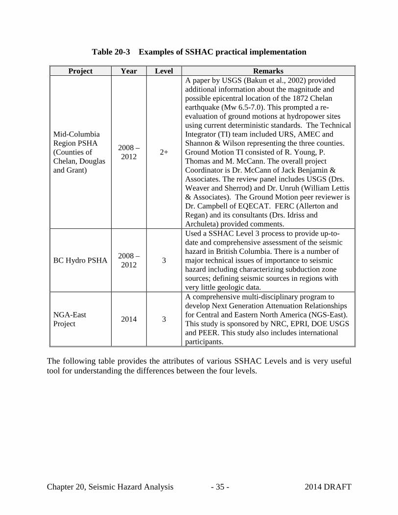
Level 3 – highly contentious; significant to hazard; and highly complex; involves a TI Level 4 - similar to a Level 3, but involves a TFI (technical facilitator/integrator) whose function is to organize panel of experts The first three less-complex levels involve an entity called the Technical Integrator (TI) who is responsible for all aspects of PSHA including analyses, specifying the input parameters and their uncertainties. The TI in Level 1 is usually a single hazard analyst but the TI need not be restricted to a single person. The TI in Level 2 is part of the TI team. The highest level (Level 4) makes use of the Technical Facilitator/Integrator (TI) whose role is to elucidate, aggregate, evaluate and integrate the opinions of experts. For most technical issues, the TI and TFI are envisioned as roles that may be filled by one person or in the TFI case by a small team. A consultant trained in the PSHA process may fulfill the role of the TI in Level 1 and 2, however, there are very few individual capable of conducting a Level 3 or 4 PSHA. The consultant must be technically independent, (not being the proponent of any specific model); have general knowledge of the statistical, geological and geophysical analysis tools used in PSHA and by the experts and have demonstrated the ability to socially interact positively with a group of engineers and scientists with different views. Table 20-3 shows examples of SSHAC Guidelines implementation that are relevant to hydro projects.
Chapter 20, Seismic Hazard Analysis - 35 - 2014 DRAFT
Table 20-3 Examples of SSHAC practical implementation Project Year Level Remarks
Mid-Columbia Region PSHA (Counties of Chelan, Douglas and Grant)
2008 – 2012 2+
A paper by USGS (Bakun et al., 2002) provided additional information about the magnitude and possible epicentral location of the 1872 Chelan earthquake (Mw 6.5-7.0). This prompted a re-evaluation of ground motions at hydropower sites using current deterministic standards. The Technical Integrator (TI) team included URS, AMEC and Shannon & Wilson representing the three counties. Ground Motion TI consisted of R. Young, P. Thomas and M. McCann. The overall project Coordinator is Dr. McCann of Jack Benjamin & Associates. The review panel includes USGS (Drs. Weaver and Sherrod) and Dr. Unruh (William Lettis & Associates). The Ground Motion peer reviewer is Dr. Campbell of EQECAT. FERC (Allerton and Regan) and its consultants (Drs. Idriss and Archuleta) provided comments.
BC Hydro PSHA 2008 – 2012 3
Used a SSHAC Level 3 process to provide up-to-date and comprehensive assessment of the seismic hazard in British Columbia. There is a number of major technical issues of importance to seismic hazard including characterizing subduction zone sources; defining seismic sources in regions with very little geologic data.
NGA-East Project 2014 3
A comprehensive multi-disciplinary program to develop Next Generation Attenuation Relationships for Central and Eastern North America (NGS-East). This study is sponsored by NRC, EPRI, DOE USGS and PEER. This study also includes international participants.
The following table provides the attributes of various SSHAC Levels and is very useful tool for understanding the differences between the four levels.

Table 20-4 Attributes of Various SSHAC Levels
Chapter 20, Seismic Hazard Analysis - 36 - 2014 DRAFT
SSHAC Level
Level 1
Level
2
Level 3
Level 4
Number of participants
• Project Manager • Small TI team • Peer reviewers • Hazard calculation team
• Project Manager • Small TI team • Peer reviewers • Hazard calculation team • Resource experts • Proponent experts
• Project Manager • Project TI • Larger TI team • Peer reviewers • Resource experts • Proponent experts • Data team • Hazard calculation team
• Project Manager • Project TFI • Small TFI team • Panel(s) of evaluator experts • Peer reviewers • Resource experts • Proponent experts • Data team • Hazard calculation team
Interaction
• Limited or no contact with proponent and resource experts
• Proponent and resource experts contacted individually
• Proponent and resource experts interact with TI Team in facilitated workshops
• Proponent and resource experts interact with evaluator experts in facilitated workshops
Peer review • Late stage • Late stage • Participatory • Participatory
Ownership • TI Team • TI Team • TI Team • TFI team and evaluator experts
Transparency
• Dependent on documentation
• Dependent on documentation • Interested parties can view interactions at workshops
• Participatory peer reviewers observe workshops, participate in Workshop #3
• Dependent on documentation
• Interested parties can view interactions at workshops
• Participatory peer reviewers observe workshops, participate in Workshop #3
• Dependent on documentation
Regulatory Assurance*
• Limited or no interaction with proponent and resource experts reduces confidence
• Depends on TI team and degree to which data, models, and methods are readily available
• Individual interaction with proponent and resource experts increases confidence over Level 1
• Depends on TI team; degree to which data, models, and methods are readily available; and success in obtaining additional information and understanding from individual interactions
• Interaction among proponent, resource, and evaluator experts in facilitated workshops greatly increases confidence over Level 2
• Documentation of evaluation and integration process by TI Team key to high levels of confidence
• Interaction among proponent, resource, and evaluator experts in facilitated workshops greatly increases confidence over Level 2
• Documentation of evaluation and integration process by evaluator experts key to high levels of confidence
*Regulatory Assurance is defined as confidence that views of the larger technical community has been considered and that the center, body, and range of technically defensible interpretations has been represented.
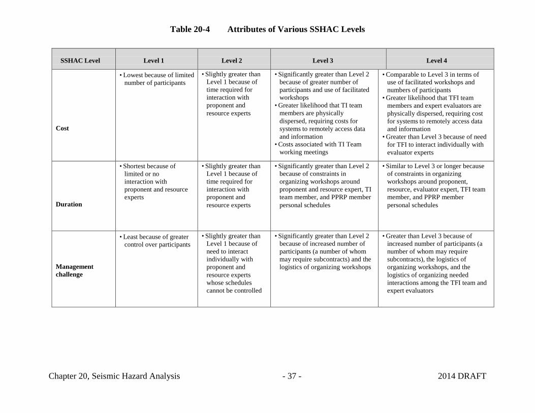
Table 20-4 Attributes of Various SSHAC Levels
Chapter 20, Seismic Hazard Analysis - 37 - 2014 DRAFT
SSHAC Level
Level 1
Level 2
Level 3
Level 4
Cost
• Lowest because of limited number of participants
• Slightly greater than Level 1 because of time required for interaction with proponent and resource experts
• Significantly greater than Level 2 because of greater number of participants and use of facilitated workshops
• Greater likelihood that TI team members are physically dispersed, requiring costs for systems to remotely access data and information
• Costs associated with TI Team working meetings
• Comparable to Level 3 in terms of use of facilitated workshops and numbers of participants
• Greater likelihood that TFI team members and expert evaluators are physically dispersed, requiring cost for systems to remotely access data and information
• Greater than Level 3 because of need for TFI to interact individually with evaluator experts
Duration
• Shortest because of limited or no interaction with proponent and resource experts
• Slightly greater than Level 1 because of time required for interaction with proponent and resource experts
• Significantly greater than Level 2 because of constraints in organizing workshops around proponent and resource expert, TI team member, and PPRP member personal schedules
• Similar to Level 3 or longer because of constraints in organizing workshops around proponent, resource, evaluator expert, TFI team member, and PPRP member personal schedules
Management challenge
• Least because of greater control over participants
• Slightly greater than Level 1 because of need to interact individually with proponent and resource experts whose schedules cannot be controlled
• Significantly greater than Level 2 because of increased number of participants (a number of whom may require subcontracts) and the logistics of organizing workshops
• Greater than Level 3 because of increased number of participants (a number of whom may require subcontracts), the logistics of organizing workshops, and the logistics of organizing needed interactions among the TFI team and expert evaluators

Chapter 20, Seismic Hazard Analysis - 38 - 2014 DRAFT
Table 20-3 is provided for reference and strict adherence to its guidance is not required. For most technical issues that arise in a typical PSHA for dam safety, the levels of effort described above can be modified with considerations of the consequence of dam failure, ground motion level, probability of dam failure, and uncertainty. For instance, a Level 1 SSHAC analysis may provide sufficient information to determine the need for permanent risk reduction, even for higher consequence and likelihood dams. This situation would occur if the probability of loading and failure is adequate to show clearly what and how to remediate the dam, without further analysis. On the other hand, a dam with lesser consequence, but high uncertainty might suggest the need for a higher level SSHAC analysis to verify the analyses if more certainty is required to support a decision. Also note that Level 4 SSHAC PSHAs are very rare and might only occur if most or all of the following factors apply: high likelihood of failure, high uncertainty, high cost of remediation, and the consequences include high predicted life loss and possible national and international implications. As discussed in Chapter R24 of the RIDM EGs, the reference to the SSHAC process is not intended to imply that all SSHAC procedures are required to be used for all PSHAs. SSHAC procedures need to be applied using judgment. The FERC can be consulted if necessary.
R20.12 Using PSHA Curves
R20.12.1 Fragility Analyses
The vulnerability of a dam against seismic loading can be quantified through a process called fragility analysis. In a seismic fragility analysis, the probability of dam failure in terms of excessive deformation or structural damage can be quantified by taking into account the initiating earthquake event at different loading probabilities. The fragility analysis also incorporates the response and type of structure (e.g. concrete vs. earthfill embankment dam). Table 20-5 below shows the typical steps for using a fragility analysis a risk analysis. In this example, the dam failure defined in terms of the uncontrolled rapid release of water (URRW) resulting from seismic events is determined using the following parameters:
1) Hazard Curve - rate of exceedance at which specific ground motion levels are exceeded. The hazard curve is a product of PSHA.
2) Dam Fragility Curve – the probability that the dam will develop into a URRW state given the ground motion shaking level. Dam fragility curve relates the probability of URRW versus a range of ground motion scenarios (e.g. peak ground acceleration (PGA) levels).

Chapter 20, Seismic Hazard Analysis - 39 - 2014 DRAFT
Table 20-4 Typical procedures for developing the probability of failure using a dam fragility analysis
Step 1 Perform PSHA and Develop Hazard Curve
Step 2 Obtain Deaggregation Data and Calculate Fractional Contribution to Spectral Acceleration
Step 3 Determine Ground Motion Annual Rate of Exceedance (Return Period)
Step 4 Define Potential Failure Mode (PFM) (Sliding, Liquefaction, Deformation, Cracking, etc.)
Step 5 Develop Cross-Section. Compile Material Properties incl. mean and standard deviation
Step 6 Conduct a Dynamic Response Analysis using Finite Element Method or equivalent.
Step 7 Assess the Probability of Failure for a Given PFM
Step 8 Determine Conditional Probability of URRW at Different Levels of Ground Motion
Note that the other RIDM EG Chapters describe how to analyze the probability of dam failure and complete dam fragility analyses, if appropriate.
R20.12.2 Simplified Method for PSHA One possible simplified method would be to use risk-targeted ground motions developed by using a ‘tolerable’ risk criteria, as was recently used for evaluating the Mid-Columbia PSHA. This method can be considered an interim method prior to using fully quantitative risk analysis and uses a tolerable risk criteria developed by the USACE. The risk-targeted ground motion is estimated in terms of the probability of dam failure with its resultant downstream consequence of uncontrolled release of reservoir water. This is analogous to the ASCE 7-10 procedures for determining risk-targeted ground motions aimed to have a uniform risk of building collapse. To calculate risk-targeted ground motions with the aim of achieving uniformity across regulated hydro facilities, the steps involved: calculating the seismic hazard from PSHA, integrating fragility and hazard curves with the consequence of failure, and adjusting the ground motion estimate. The procedure is repeated until the estimated input ground motion produces the desired tolerable risk.
Figure 20-8 illustrates the simplified methodology for evaluating the seismic safety of a dam or its structural component under a single seismic-related potential failure mode (e.g. liquefaction, deformation, slope instability, etc.). The methodology assumes that site response analysis, whether it is site-specific or implicit from the hazard analysis, is

Chapter 20, Seismic Hazard Analysis - 40 - 2014 DRAFT
“Free-Field” Hazard Estimate
Return Period
Spectral Acceleration
Spectral Acceleration
NO
YES
Damage
Probability
Probability
Risk Plot
performed prior to the fragility analysis. Note that in order to fully analyze the overall risk to a hydro project, the loading conditions and fragility curves for all project features and potential failure modes must be determined. This method typically assumes that the seismic risk takes up only part of the overall risk, and may not be adequate if this assumption is invalid.
Figure 20-8 Risk-targeted ground motion based on a simplified methodology.
Hazard Curve
Probability of Dam Failure
Fragility Curve
Consequence Curve
Calculated risk satisfies the tolerable risk guideline?
Select New Ground Motion Return Period
URRRW*
Risk-Targeted Ground Motion
Site
Fatalities N
Step 1 – Establish Seismic Load Uncertainty
Step 2 – Establish Dam Fragility and Consequence
Step 3 – Estimate Risk

Chapter 20, Seismic Hazard Analysis - 41 - 2014 DRAFT
R20.13 RIDM Seismic Methodology
In summary, the RIDM methodology for seismic safety evaluation consists of the following steps:
• Seismic Hazard – Analyze the seismic hazards at a site using a PSHA
approach. Expected output from a PSHA includes hazard curves, deaggregation, uniform hazard spectrum and conditional mean spectrum (CMS). CMS is the preferred representation of realistic ground motions for structural analysis.
• Site Response – If required, perform site-specific site response analysis as input to fragility analysis. Site response analysis requires information such as shear wave velocities, dynamic material properties, amplification factors, topography, etc.
• Seismic Structural Analysis – Perform seismic structural analyses including fragility analysis (as needed) for individual or multiple failure modes and determine the probability of failure leading to a dam breach and an uncontrolled release of reservoir water (URRW).
• Consequence – Quantify the potential loss-of-life and economic damages
resulting from URRW.
• Risk – Calculate the annualized life loss or cumulative life loss for all PFMs as shown on fN or FN charts. Evaluate the acceptability of the result using ALARP principles.
Chapter 20, Appendix A - 1 - 2014 DRAFT
APPENDIX A
Examples of PSHA
Introduction
This appendix describes the types of results that should be included in a modern probabilistic seismic hazard analysis and in the development of time histories for dynamic analyses. In this appendix, the standard equations for conducting the PSHA and time history development are not given. Rather, the presentation of the results is described. The details for developing realistic scenario earthquake spectra are described since this is not part of standard PSHA practice. The focus of this appendix is on the presentation and characterization of the hazard results, and not on the source and ground motion characterizations. Two sites, one in a high activity region (San Francisco Bay Area) and one in a moderate activity region (Pacific Northwest), are used as examples. SOURCE CHARACTERIZATION The source characterization should include a description of the key sources and a map of faults and source zones and the historical seismicity. There should also be a table that clearly shows the fault and source zone parameters used in the PSHA, including alternatives models and parameter values with their associated weights. Maximum Magnitude Inconsistent use of terminology is a cause of confusion in many PSHA reports. In listing the fault and source zone parameters, the term "maximum magnitude" is often used for both the true maximum magnitude and for the mean magnitude from full rupture of a fault. For source zones, the maximum magnitude is the largest magnitude that can occur in the source zone. If an exponential distribution is used for the magnitudes (e.g. Gutenberg-Richter model), then the maximum magnitude is the magnitude at which the exponential distribution is truncated. For faults, the dimension of the fault (length or area) is typically used to estimate the mean magnitude for full rupture of the fault. This mean magnitude is better described as the "mean characteristic magnitude" and not as the maximum magnitude because the PSHA will typically consider a range of ranges about this mean magnitude to account for the variability of the magnitude for a given rupture dimension. For example, the widely used Youngs and Coppersmith (1985) model for the magnitude distribution has the characteristic part of the model centered on the mean characteristic magnitude and the maximum magnitude is 0.25 units larger.

Chapter 20, Appendix A - 2 - 2014 DRAFT
Attenuation Relations In most cases, the attenuation relations are selected from existing models for the appropriate tectonic regime (shallow crustal earthquakes in active tectonic regions, shallow crustal earthquakes in stable continental regions, or subduction zone earthquakes). Alternative models that are considered applicable should be used to capture the epistemic uncertainty in the ground motion models. The PSHA report needs to describe the weights used for each alternative model. In some cases, new ground motion models are derived for a specific project using either empirical data or numerical simulations. The most commonly used numerical simulation procedure is the point source stochastic model (Boore, 2006). If new project-specific ground motion models are derived, then a description of the development of the new model should be included. Hazard Results The basic result of a PSHA is the hazard curve which shows the probability of exceeding a ground motion for a range of ground motion values. As a minimum, the hazard should be shown for a least two spectral periods: one short period, such as PGA, and one long period, such as T=2 sec. The selection of the spectral periods should consider the period of the structure. The mean hazard curves should be plotted to show the hazard curve from each source and the total hazard curve to provide insight into which sources are most important. The mean hazard curves should also be shown in terms of the total hazard using each attenuation relation separately to show the impact of the different ground motion models. Finally, the fractiles of the hazard should be plotted to show the range of hazard that arises due to the uncertainty in the characterization of the sources and ground motion. Deaggregation The hazard curve gives the combined effect of all magnitudes and distances on the probability of exceeding a given ground motion level. Since all of the sources, magnitudes, and distances are mixed together, it is difficult to get an intuitive understanding of what is controlling the hazard from the hazard curve by itself. To provide insight into what events are the most important for the hazard at a given ground motion level, the hazard curve is broken down into its contributions from different earthquake scenarios. This process is called deaggregation. In a hazard calculation, there is a large number of scenarios considered (e.g. thousands or millions of scenarios). To reduce this large number of scenarios to a manageable number, similar scenarios are grouped together. A key issue is what constitutes “similar”
Chapter 20, Appendix A - 3 - 2014 DRAFT
scenarios. Typically, little thought has been given to the grouping of the scenarios. Most hazard studies use equal spacing in magnitude space and distance space. This may not be appropriate for a specific project. The selection of the grouping of scenarios should be defined by the engineers conducting the analysis of the structure. In a deaggregation, the fractional contribution of different scenario groups to the total hazard is computed. The most common form of deaggregation is a two-dimensional deaggregation in magnitude and distance bins. The dominant scenario can be characterized by an average of the deaggregation. Two types of averages are considered: the mean and the mode. The mean magnitude and mean distance are the weighted averages with the weights given by the deaggregation. The mean has advantages in that it is defined unambiguously and is simple to compute. The disadvantage is that it may give a value that does not correspond to a realistic scenario The mode is the most likely value. It is given by the scenario group that has the largest deaggregation value. The mode has the advantage it will always correspond to a realistic source. The disadvantage is that the mode depends on the grouping of the scenarios, so it is not robust. It is useful to plot the deaggregation both by M-R bin and the mean M, R, and epsilon. Uniform Hazard Spectra A common method for developing design spectra based on the probabilistic approach is uniform hazard spectra. A uniform hazard spectrum (UHS) is developed by first computing the hazard at a suite of spectral periods using response spectral attenuation relations. That is, the hazard is computed independently for each spectral period. For a selected return period, the ground motion for each spectral period is measured from the hazard curves. These ground motions are then plotted at their respective spectral periods to form the uniform hazard spectrum. The term “uniform hazard spectrum” is used because there is an equal probability of exceeding the ground motion at any period. Since the hazard is computed independently for each spectral period, in general, a uniform hazard spectrum does not represent the spectrum of any single earthquake. It is common to find that the short period (T<0.2 sec) ground motions are controlled by nearby moderate magnitude earthquakes, whereas, the long period (T>1 sec) ground motions are controlled by distant large magnitude earthquakes. The “mixing” of earthquakes in the UHS is often cited as a disadvantage of PSHA. There is nothing in the PSHA method that requires using a UHS. A suite of realistic

Chapter 20, Appendix A - 4 - 2014 DRAFT
scenario earthquake spectra can be developed as described below. The reason for using a UHS rather than using multiple spectra for the individual scenarios is to reduce the number of engineering analyses required. A deterministic analysis has the same issue. If one deterministic scenario leads to the largest spectral values for long spectral periods and a different deterministic scenario leads to the largest spectral values for short spectral periods, a single design spectrum that envelopes the two deterministic spectra could be developed. If such an envelope is used, then the deterministic design spectrum also does not represent a single earthquake. The choice of using a UHS rather than multiple spectra for the different scenarios is the decision of the engineering analyst, not the hazard analyst. The engineering analyst should determine if it is worth the additional analysis costs to avoid exciting a broad period range in a single evaluation. The hazard report should include the UHS as well as the scenario spectra described below. Spectra for Scenario Earthquakes In addition to the UHS, realistic spectra for scenario earthquakes should be developed. Two different procedures for developing scenario earthquake spectra are described below. Both methods start with the identification of the controlling earthquake scenarios (magnitude, distance) from the deaggregation plots. As noted above, the controlling earthquakes will change as a function of the spectral period. Median Spectral Shape The most common procedure used for developing scenario earthquake spectra given the results of a PSHA is to use the median spectral shape (Sa/PGA) for the earthquake scenario from the deaggregation and then scale the median spectral shape so that it matches the UHS at the specified return period and spectral period. This process is repeated for a suite of spectral periods (e.g. T=0.2 sec, T=1 sec, T=2.0 sec). The envelope of the resulting scenario spectra become equal to the UHS if a full range of spectral periods of the scenarios is included. This avoids the problem of mixing different earthquake scenarios that control the short and long period parts of the UHS. A short-coming of the median spectral shape method is that it assumes that the variability of the ground motion is fully correlated over all spectral periods. For example, if the UHS at a specified spectral period and return period corresponds to the median plus 1 sigma ground motion for the scenario (epsilon =1), then by scaling the median spectral shape, we are using the median plus 1 sigma ground motion at each period. Spectra from real earthquakes will have peaks and troughs so we don't expect that the spectrum at all periods will be at the median plus 1 sigma level. This short-coming is addressed in the second method.

Chapter 20, Appendix A - 5 - 2014 DRAFT
Expected Spectral Shape In this method, the expected spectral shape for the scenario earthquake is computed. In this case, the expected spectral shape depends not only on the scenario earthquake, but also on the epsilon value required to scale the scenario spectrum to the UHS. Again, consider a case in which the UHS is one standard deviation above the median spectral acceleration from the scenario earthquake for a period of 2 sec. At other spectral periods, the chance that the ground motion will also be at the 1 sigma level decreases as the spectral period moves further from 2 sec. To compute the expected spectral shape, we need to consider the correlation of the variability of the ground motion at different spectral periods. (This is the correlation of the variability of the ground motion, not the correlation of the median values). In the past, this correlation has not been commonly included as part of the ground motion model, but the correlation tends to be only weakly dependent on the data set. That is, special studies that have developed this correlation can be applied to a range of ground motion models. Below, the equations for implementing this progress are given. First, we need to compute the number of standard deviations, εU(To,TRP), needed to scale the median scenario spectral value to the UHS at a spectral period, To, and for a return period, TRP. This is given by
where and are the median and standard deviation of the ground motion for the scenario earthquake from the attenuation relations. The expected epsilon at other spectral periods is given by
where c is the square root of the correlation coefficient of the residuals at period T and To. An example of the values of coefficient c computed from the PEER strong motion data for M>6.5 for rock sites are listed in Table 20B-1 for reference periods of 0.2, 1.0, and 2.0. The expected spectrum for the scenario earthquake is then given by
This expected spectrum for the scenario earthquake is called the "conditional mean spectrum" by Baker and Cornell (2006).
εU (To ,TRP )=ln UHS(To ,TRP )( )− ln ˆ S a(M ,R,To)( )
σ (To ,M )
ˆ S a(M ,R,To)
σ (To ,M )
ˆ ε (T )=cεU (To ,TRP )
Sa(T )= ˆ S a(M ,R,To) exp ˆ ε (To,TRP )σ (To ,M )( )

Chapter 20, Appendix A - 6 - 2014 DRAFT
Table 20B-1. Example of the Slope of the Relation Between Epsilons for the Expected Spectral Shape
Period (Sec) To=0.2 To=1.0 To=2.0 0.0 0.91 0.68 0.43
0.075 0.91 0.54 0.31 0.1 0.91 0.50 0.27 0.2 1.00 0.48 0.26 0.3 0.93 0.63 0.39 0.4 0.84 0.71 0.45 0.5 0.71 0.77 0.52 0.75 0.62 0.92 0.66 1.0 0.45 1.00 0.76 1.5 0.37 0.87 0.85 2.0 0.26 0.81 1.00 3.0 0.24 0.77 0.94
Time Histories
Time histories are developed using the spectral matching approach for the Pacific Northwest example and using the scaling approach for the northern California example. The basis for selecting the reference time histories should be described. One draw-back of using the expected scenario spectra is that additional time histories will be required. If the project uses the average response of 7 time histories, then 7 time histories are needed for each scenario spectrum. The average response is computed for each scenario and then the larger response from the two scenario is used. If the scaling procedure is used, then time history report should list the scale factors and include the following plots:
Acceleration, velocity, and displacement seismograms for the scaled time histories, Fourier amplitude spectra for the scaled time histories, Comparison of the spectra of the scaled time histories with the design spectrum.
If the spectral matching procedure is used, then there are additional plots that are needed to check that the modified time history is still appropriate (e.g. check that the spectral matching has not lead to an unrealistic ground motion). The acceleration, velocity, and displacement seismograms of the modified ground motion should have the same gross non-stationary characteristics as the reference motion. For spectral matching, the time history report should include the following plots:

Chapter 20, Appendix A - 7 - 2014 DRAFT
Acceleration, velocity, and displacement seismograms for the reference and modified time histories,
Fourier amplitude spectra for the reference and modified time histories, Comparison of Husid plots (normalized arias intensity) for the reference and modified
time histories, Comparison of the spectra of the reference and modified time histories with the
scenario earthquake spectrum.

Chapter 20, Appendix A - 8 - 2014 DRAFT
Pacific Northwest Example
A site located in northwestern Washington is used as an example. In this example, a return period of 2000 years is used. This return period is just for this example and does not imply this is this an accepted return period for dams. The selection of the return period for design ground motions for dams has not been resolved.
Source Characterization
For this example, a simplified source characterization is used. Five sources are considered: the Cascadia interface, the Juan de Fuca intra-slab, the Seattle fault, the Hood Canal fault, and a background zone. The location of the site with respect to the faults and source zones is shown in Figure 20B-1. The parameters used for the sources are given in Tables 20B-2a and -2b. These are based on the source models used by PG&E (2001, 2002a), Adams and Halchuk (2003), and the USGS as part of the national hazard maps. The objective of these examples is on the presentation of the hazard results, so a detailed description of the source models is not included here. In a complete hazard study, such detailed source descriptions should be included.
Ground Motion Models
In the Pacific Northwest, both crustal and subduction earthquakes need to be considered. These two tectonic classes of earthquakes require separate ground motion models. For the crustal sources, the five NGA models recently developed as part of the PEER/Lifelines program are used. These new ground motion models include Abrahamson and Silva (2007), Boore and Atkinson (2006), Campbell and Bozorgnia (2006), Chiou and Youngs (2006), and Idriss (2007). For the Idriss model, the rock site class is used. For the other four models, a VS30 of 600 m/s is used. These five models are given equal weight. For the subduction earthquakes, two models are used: Youngs et al (1997) and Atkinson and Boore (2003). For the Youngs et al model, the rock relation is used. For the Atkinson and Boore model, NEHRP site class C is used. The two models are given equal weight.

Chapter 20, Appendix A - 9 - 2014 DRAFT
Table 20B-2a Source parameters for fault sources
Mean Characteristic
Magnitude
Recurrence Interval (yrs)
of Characteristic
Eqk
Slip-Rates (mm/yr)
Style-of-Faulting
Cascadia 8.2 (0.105) 8.4 (0.22) 8.5 (0.075) 8.6 (0.07) 8.7 (0.205) 8.8 (0.074) 8.9 (0.175) 9.1 (0.075)
230 (0.05) 300 (0.15) 340 (0.05) 370 (0.15) 500 (0.45) 660 (0.15)
Interface
Seattle Fault 6.9 (0.2) 7.1 (0.6) 7.3 (0.2)
5000 (0.5) 0.7 (0.25) 1.1 (0.25)
Reverse
Hood Canal fault
7.0 (1.0) 0.1 (1.0) Strike-slip
Table 20B-2b Source parameters for areal source zones Source b N(M>5) b,N wt Mmax Top
(km) Bottom
(km) Style-of-Faulting
Juan de Fuca Plate Onshore
Deep
1.119 0.899 0.678
0.0007 0.0035 0.0159
(0.16) (0.68) (0.16)
6.7 (0.3) 7.1
(0.6) 7.3
(0.1)
40 80 Intra-slab
Puget Sound Deep
0.547 0.491 0.430
0.0650 0.0985 0.1770
(0.16) (0.68) (0.16)
6.9 (0.3) 7.1
(0.6) 7.3
(0.1)
50 90 Intra-slab
Cascades Mtns
Background
0.92 0.87 0.83
0.0019 0.0028 0.0039
(0.16) (0.68) (0.16)
6.5 (0.5) 7.0
(0.5)
0 15 Reverse
Hazard Results
The basic hazard results are shown in Figures 20B-2a and -2b for PGA and T=2 sec, respectively. These figures also show how each source contributes to the hazard. For PGA (Figure 20B-2a), the deep earthquakes in the Juan de Fuca plate slab have the largest contribution to the hazard. The Cascadia source has about one-half of the contribution of the Juan de Fuca source. For long spectral periods (e.g. T=2 sec), the Cascadia source dominates the hazard at long return periods, but the Juan de Fuca source

Chapter 20, Appendix A - 10 - 2014 DRAFT
is still dominant at short return periods (less than 200 years). The sensitivity of the hazard to the attenuation relations is shown in Figures 20B-3a and -3b for PGA and T=2 sec, respectively. Since there are two classes of attenuation relations (subduction and crustal), the sensitivity is shown in terms of each class. In the top frame of each figure, the sensitivity to the subduction attenuation relation is shown. In the lower frame, the sensitivity to the crustal attenuation relation is shown. For both PGA and T=2 sec, the hazard has a strong dependence on the subduction attenuation relation, but not on the crustal attenuation relation. The epistemic uncertainty in the hazard is shown in Figures 20B-4a and -4b for PGA and T=2 sec, respectively. The mean hazard is the weighted average of the hazard (y-axis) computed for each combination of alternative models. The fractiles represent the range of the hazard for the alternative models. In this case, the range of the fractiles is dominated by the epistemic uncertainty in the subduction attenuation relations. A range of a factor of 10 from the 5th to the 95th fractile is common in regions with large uncertainty in the ground motion model. The UHS for return periods of 500, 1000, 2000, and 5000 years is shown in Figure 20B-5a. This figure also compares the Cascadia (M9, R=55 km) ground motions (median and 84th percentile) for the MCE as used in deterministic analyses. In this example, the deterministic spectra are shown separately for the two subduction attenuation relations used since these two model have significant differences. The deterministic spectra from the two subduction models are similar at long periods for which the Cascadia source dominates the hazard. Figure 20B-5b compares the UHS to the Juan de Fuca (M7.5, R=40 km) ground motions for the MCE. For this scenario, the two subduction models are similar at short periods, but the Atkinson & Boore model leads to much larger ground motions at long periods. The deaggregation for a return period of 2000 years is shown in Figure 20B-6a and -6b for PGA and T=2 sec, respectively. Figure 20B-6a shows that for PGA, the mode of the deaggregation is M7.0-7.5 at distances of 50-80 km. Figure 20B-6b shows that for T=2 sec, the mode of the deaggregation is M8.5-9.0 at distances of 50-60 km. In addition to the mode, the deaggregation can be characterized by the mean magnitude, distance, and epsilon. These mean values are shown in Figure 20B-7 as a function of return period for PGA and T=2 sec. This figure shows that the mean magnitude for PGA increases as the return period increases from 100 to 500 years, but for longer return periods, the mean magnitude does not increase. For return periods greater than 500 years, the mean distance continues to decrease and the mean epsilon increases. In contrast to the PGA, For T=2 sec, the mean magnitude continues to increase as the return period increases from 100 to 10,000 years.

Chapter 20, Appendix A - 11 - 2014 DRAFT
Expected Spectra for Scenario Earthquakes From the deaggregation, the following scenario earthquakes were selected: Source M Distance (km) To (sec) Juan de Fuca 7.3 50 km 0.2 Cascadia 8.8 55 km 2.0 The expected spectra are developed for these of these events. First, the median and standard deviation for the two scenarios listed above are computed using the two subduction ground motion models. The average of the median and the standard deviation for the two scenario earthquakes are listed in Tables 20B-4a and -4b. Next, the number of standard deviations needed to scale the median Sa to the UHS is determined. This value, εU, is shown in Table 20B-3. The expected epsilon values at the other spectral periods are then computed (fifth column in Tables 20B-4a and -4b) and the spectrum is then computed (sixth column in Tables 20B-5a and -5b). The expected spectra for the scenarios are compared to the UHS in Figure 20B-8. This figure shows that the expected spectrum falls below the UHS at periods away from the reference period. A suite of these expected spectra will be enveloped by the UHS. The expected spectra are realistic ground motions for a future earthquake. To limit the number of scenarios considered, these expected spectra will need to be broadened so that they cover the UHS with a small number of scenarios. To limit the number of scenarios considered, these expected spectra can be broadened so that they cover the UHS with a small number of scenarios. As an example, the two expected scenarios are broadened into two design spectra in Figure 20B-9. The engineer conducting the analysis of the structure needs to determine to what degree it is worth broadening the expected spectra to reduce the number of scenarios considered.
Table 20B-3. Computation of the epsilon needed to match the UHS.
Period (sec)
UHS 2000 Yr
(g) Median Sa(g) σ εU
0.2 0.946 0.439 0.682 1.126 2.0 0.210 0.096 0.766 1.021
Table 20B-4a Development for the expected spectrum for T=0.2 sec and a return period
of 2000 years.
Period (Sec) c
(To=0.2) Median Sa(g) σ
Expected Spectrum
(g) 0.00 0.91 0.192 0.625 1.024 0.364
0.075 0.91 0.269 0.648 1.024 0.522 0.10 0.91 0.314 0.671 1.024 0.624 0.20 1.00 0.439 0.682 1.126 0.947
ˆ ε

Chapter 20, Appendix A - 12 - 2014 DRAFT
0.30 0.93 0.419 0.691 1.047 0.864 0.40 0.84 0.400 0.694 0.946 0.771 0.50 0.71 0.389 0.706 0.799 0.683 0.75 0.62 0.286 0.720 0.698 0.472 1.00 0.45 0.218 0.751 0.507 0.319 1.50 0.37 0.147 0.770 0.417 0.202 2.00 0.26 0.107 0.801 0.293 0.135 3.00 0.24 0.050 0.874 0.270 0.063
Table 20B-4b Development for the expected spectrum for T=2.0 sec and a return period of 2000
years.
Period (Sec) c
(To=2.0) Median Sa(g) σ
Expected Spectrum
(g) 0.00 0.43 0.144 0.590 0.439 0.186
0.075 0.31 0.211 0.611 0.317 0.256 0.10 0.27 0.237 0.636 0.276 0.282 0.20 0.26 0.320 0.647 0.266 0.380 0.30 0.39 0.321 0.650 0.399 0.416 0.40 0.45 0.361 0.659 0.460 0.488 0.50 0.52 0.346 0.676 0.531 0.495 0.75 0.66 0.248 0.696 0.674 0.396 1.00 0.76 0.188 0.716 0.777 0.327 1.50 0.85 0.130 0.742 0.869 0.248 2.00 1.00 0.096 0.766 1.022 0.211 3.00 0.94 0.037 0.839 0.961 0.082
ˆ ε

Chapter 20, Appendix A - 13 - 2014 DRAFT
Figure 20B-1. Faults and sources considered in the example.

Chapter 20, Appendix A - 14 - 2014 DRAFT
Figure 2a. Contribution to the PGA hazard by source.
Figure 20B-2b. Contribution to the T=2 sec hazard by source
0.0001
0.001
0.01
0.1
0 0.1 0.2 0.3 0.4 0.5 0.6 0.7
Annu
al P
roba
bilit
y of
Bei
ng E
xcee
ded
Peak Acceleration (g)
Cascadia
Seattle Fault
Hood Canal fault
Juan de Fuca (Deep)
Background
Total
0.0001
0.001
0.01
0.1
0 0.05 0.1 0.15 0.2 0.25 0.3 0.35 0.4
Ann
ual P
roba
bilit
y of
Bei
ng E
xcee
ded
Spectral Acceleration (g)
Cascadia
Seattle Fault
Hood Canal fault
Juan de Fuca (Deep)
Background
Total

Chapter 20, Appendix A - 15 - 2014 DRAFT
Figure 20B-3a Sensitivity of PGA hazard to attenuation relation.
Top frame: subduction models. Bottom frame: crustal models.
0.0001
0.001
0.01
0.1
0 0.1 0.2 0.3 0.4 0.5 0.6 0.7 0.8
Annu
al P
roba
bilit
y of
Bei
ng E
xcee
ded
Peak Acceleration (g)
Youngs et al
Atkinson & Boore
0.0001
0.001
0.01
0.1
0 0.1 0.2 0.3 0.4 0.5 0.6 0.7 0.8
Annu
al P
roba
bilit
y of
Bei
ng E
xcee
ded
Peak Acceleration (g)
Abrahamson & Silva
Chiou & Youngs
Boore & Atkinson
Campbell & Bozorgnia
Idriss

Chapter 20, Appendix A - 16 - 2014 DRAFT
Figure 20B-3b. Sensitivity of T=2 sec hazard to attenuation relation.
Top frame: subduction models. Bottom frame: crustal models
0.0001
0.001
0.01
0.1
0 0.05 0.1 0.15 0.2 0.25 0.3 0.35 0.4 0.45 0.5
Annu
al P
roba
bilit
y of
Bei
ng E
xcee
ded
Spectral Acceleration (g)
Youngs et al
Atkinson & Boore
0.0001
0.001
0.01
0.1
0 0.05 0.1 0.15 0.2 0.25 0.3 0.35 0.4 0.45 0.5
Annu
al P
roba
bilit
y of
Bei
ng E
xcee
ded
Spectral Acceleration (g)
Abrahamson & Silva
Chiou & Youngs
Boore & Atkinson
Campbell & Bozorgnia
Idriss

Chapter 20, Appendix A - 17 - 2014 DRAFT
Figure 20B-4a. Uncertainty fractiles of the PGA hazard
Figure 20B-4b. Uncertainty fractiles of the T=2 sec hazard
0.0001
0.001
0.01
0.1
0 0.1 0.2 0.3 0.4 0.5 0.6 0.7 0.8
Prob
abili
ty o
f Bei
ng E
xcee
ded
Peak Acceleration (g)
5th
15th
50th
85th
95th
Mean
0.0001
0.001
0.01
0.1
0 0.05 0.1 0.15 0.2 0.25 0.3 0.35 0.4 0.45 0.5
Prob
abili
ty o
f Bei
ng E
xcee
ded
Peak Acceleration (g)
5th
15th
50th
85th
95th
Mean

Chapter 20, Appendix A - 18 - 2014 DRAFT
Figure 20B-5a. UHS and deterministic (MCE) spectra for the M9 Cascadia source (R=55
km).
0
0.5
1
1.5
0.01 0.1 1 10
Spe
ctra
l Acc
eler
atio
n (g
)
Period (sec)
500 Yr
1000 Yr
2000 Yr
5000 Yr
A&B Median (M9)
A&B 84th (M9)
Youngs et al median (M9)
Youngs et al 84th (M9)

Chapter 20, Appendix A - 19 - 2014 DRAFT
Figure 20B-5b. UHS and deterministic (MCE) spectra for the M7.6 Juan de Fuca source
(R=40 km).
0
0.5
1
1.5
0.01 0.1 1 10
Spe
ctra
l Acc
eler
atio
n (g
)
Period (sec)
500 Yr
1000 Yr
2000 Yr
5000 Yr
A&B Median (M7.5)
A&B 84th (M7.5)
Youngs et al Median, (M7.5)
Youngs et al 84th, (M7.5)
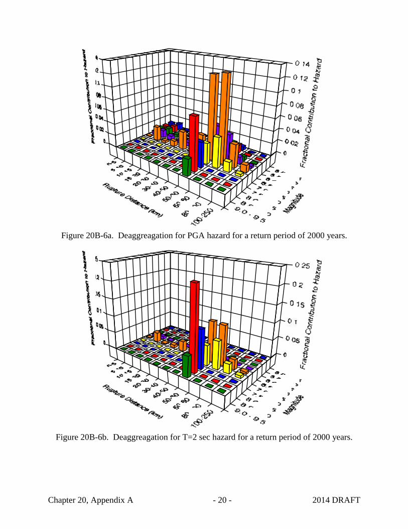
Chapter 20, Appendix A - 20 - 2014 DRAFT
Figure 20B-6a. Deaggreagation for PGA hazard for a return period of 2000 years.
Figure 20B-6b. Deaggreagation for T=2 sec hazard for a return period of 2000 years.

Chapter 20, Appendix A - 21 - 2014 DRAFT
Figure 20B-7. Return period dependence of the Mean M, R, epsilon from the deaggreagation for PGA and T=2 sec
5
5.5
6
6.5
7
7.5
8
8.5
100 1000 10000
Mea
n M
agni
tude
Return Period (yrs)
PGA
T=2 sec
01020304050607080
100 1000 10000
Mea
n D
ista
nce
(km
)
Return Period (yrs)
PGA
T=2 sec
0
0.5
1
1.5
2
2.5
3
100 1000 10000
Mea
n E
psilo
n
Return Period (yrs)
PGA
T=2 sec

Chapter 20, Appendix A - 22 - 2014 DRAFT
Figure 20B-8. Expected spectra for scenario earthquakes for the UHS at T=0.2 and T=2.0
sec.
0
0.1
0.2
0.3
0.4
0.5
0.6
0.7
0.8
0.9
1
0.01 0.1 1 10
Spec
tral A
ccel
erat
ion
(g)
Period (sec)
2000 Yr UHS
Juan de Fuca Scenario (T=0.2)
Cascadia Scenario T=2.0)

Chapter 20, Appendix A - 23 - 2014 DRAFT
Figure 20B-9. Example of broadening the expected spectra for scenario earthquakes into
a small set of design spectra.
0
0.2
0.4
0.6
0.8
1
1.2
0.01 0.1 1 10
Spe
ctra
l Acc
eler
atio
n (g
)
Period (sec)
2000 Yr UHS
Juan de Fuca Scenario (T=0.2)
Cascadia Scenario T=2.0)
Design Spectra 1
Design Spectra 2

Chapter 20, Appendix A - 24 - 2014 DRAFT
San Francisco Bay Area Example The second example is for a site located in a high seismic region. A site located in the east bay in Northern California is used as the second example. Again, a return period of 2000 years is used. Source Characterization
For this example, a simplified source characterization is used. Three fault sources are considered: the San Andreas, Hayward/Rodgers Creek, and Calaveras. The location of the site with respect to the faults is shown in Figure 20B-10. The parameters used for the sources are given in Table 20B-5. These are based on the USGS WG03 model. The objective of these examples is on the presentation of the hazard results, so a detailed description of the source models is not included here. In a complete hazard study, such detailed source descriptions should be included. Ground Motion Models
For the crustal sources, the five NGA models recently developed as part of the PEER/Lifelines program are used. These new ground motion models include Abrahamson and Silva (2007), Boore and Atkinson (2006), Campbell and Bozorgnia (2006), Chiou and Youngs (2006), and Idriss (2007). For the Idriss model, the rock site class is used. For the other four models, a VS30 of 600 m/s is used. These five models are given equal weight.

Chapter 20, Appendix A - 25 - 2014 DRAFT
Table 20B-5. Source parameters for fault sources Fault System Rupture Mean
Characteristic Magnitude
Recurrence Interval (yrs)
of Characteristic
Eqk
Style-of-Faulting
San Andreas SAS 7.03 (0.8) 6.84 (0.1) 7.22 (0.1)
1,140(0.8) 260 (0.1) 100,000 (0.1)
Strike-Slip
San Andreas SAP 7.15 (0.8) 6.95 (0.1) 7.32 (0.1)
670 (0.8) 160 (0.1) 100,000 (0.1)
Strike-Slip
San Andreas SAN 7.45 (0.8) 7.28 (0.1) 7.61 (0.1)
3,320 (0.8) 800(0.1) 100,000 (0.1)
Strike-slip
San Andreas SAO 7.29 (0.8) 7.12 (0.1) 7.44 (0.1)
3320 (0.8) 680 (0.1) 100,000 (0.1)
Strike-slip
San Andreas SAS+SAP 7.42 (0.8) 7.26 (0.1) 7.56 (0.1)
840 (0.8) 30,000 (0.1) 280 (0.1)
Strike-slip
San Andreas SAN+SAO 7.70 (0.8) 7.53 (0.1) 7.86 (0.1)
870 (0.8) 30,000 (0.1) 270 (0.1)
Strike-slip
San Andreas SAS+SAP+SAN 7.76 (0.8) 7.59 (0.1) 7.92 (0.1)
30,000 (0.8) 10,000 (0.1) 100,000 (0.1)
Strike-slip
San Andreas SAP+SAN+SAO 7.83 (0.8) 7.65 (0.1) 8.01 (0.1)
15,000 (0.8) 2700 (0.1) 100,000 (0.1)
Strike-slip
San Andreas SAS+SAP+SAN+SAO 7.90 (0.8) 7.72 (0.1) 8.10 (0.1)
620 (0.8) 10,000 (0.1) 200 (0.1)
Strike-slip
San Andreas Floating 6.9 (0.1) 410 (0.8) 7,500 (0.1) 100 (0.1)
Strike-slip
Hayward/RC HS 6.67 (0.8) 6.36 (0.1) 6.93 (0.1)
250 (0.8) 1350 (0.1) 80 (0.1)
Strike-slip
HN 6.49 (0.8) 6.18 (0.1) 6.78 (0.1)
230 (0.8) 1290 (0.1) 70 (0.1)
Strike-slip
HS+HN 6.91 (0.8) 6.68 (0.1) 7.12 (0.1)
340 (0.8) 1560 (0.1) 110 (0.1)
Strike-slip
RC 6.98 (0.8) 6.81 (0.1) 7.14 (0.1)
180 (0.8) 720 (0.1) 56 (0.1)
Strike-slip
HN+RC 7.11 (0.8) 6.94 (0.1) 7.28 (0.1)
1650 (0.8) 440 (0.1) 100,000 (0.1)
Strike-slip
HN+RS+RC 7.26 (0.8) 7.09 (0.1) 7.42 (0.1)
3,000(0.8) 30,000 (0.1) 900 (0.1)
Strike-slip
Floating 6.90 (1.0) 4270 (0.8) Strike-slip

Chapter 20, Appendix A - 26 - 2014 DRAFT
10,000 (0.1) 1860 (0.1)
Calaveras CS 5.79 (0.8) 5.0 (0.1) 6.14 (0.1)
125 (0.8) 40 (0.1) 100,000 (0.1)
Strike-slip
CC 6.23 (0.8) 5.75 (0.1) 6.68 (0.1)
200 (0.8) 750 (0.1) 85 (0.1)
Strike-slip
CS+CC 6.36 (0.8) 5.87 (0.1) 6.75 (0.1)
590 (0.8) 130 (0.1) 100,000 (0.1)
Strike-slip
CN 6.78 (0.8) 6.58 (0.1) 6.97 (0.1)
230 (0.8) 990 (0.1) 70 (0.1)
Strike-slip
CC+CN 6.90 (0.8) 6.68 (0.1) 7.11 (0.1)
10,000 (0.8) 820 (0.1) 100,000 (0.1)
Strike-slip
CS+CC+CN 6.93 (0.8) 6.72 (0.1) 7.14 (0.1)
1490 (0.8) 370 (0.1) 100,000 (0.1)
Strike-slip
Floating 6.20 (1.0)
390 (0.8) 1750 (0.1) 140 (0.1)
Strike-slip
CS+CC_floating 6.2 (1.0) 100 (0.8) 570 (0.1) 40 (0.1)
Strike-slip
Hazard Results
The basic hazard results are shown in Figures 20B-11a and -11b for PGA and T=1 sec, respectively. These figures also show how each source contributes to the hazard. Since the site is located close to a high activity fault, the hazard is dominated by the nearby Hayward fault at both short and long spectral periods. The sensitivity of the hazard to the attenuation relations is shown in Figures 20B-12a and -12b for PGA and T=1 sec, respectively. As the return period increases (lower annual probability), the difference due to the attenuation relation increases. This is due to the different values of the standard deviations. The epistemic uncertainty in the hazard is shown in Figures 20B-13a and -13b for PGA and T=1 sec, respectively. In this case, the range of the fractiles is dominated by the epistemic uncertainty in the subduction attenuation relations. The UHS for return periods of 500, 1000, 2000, and 5000 years is shown in Figure 20B-14. This figure also compares the Hayward MCE (M7.25, R=3.5 km) ground motions (median and 84th percentile) as used in deterministic analyses. At short spectral periods, the 84th percentile ground motion corresponds to a return period of about 700 years. This increases to a return period of 200 years at long spectral periods.

Chapter 20, Appendix A - 27 - 2014 DRAFT
The deaggregation for a return period of 2000 years is shown in Figures 20B-15a and -15b for PGA and T=1 sec, respectively. Figure 20B-15a shows that for PGA, the mode of the deaggreagation is M6.5-7.0 at a distance of 0-5 km. Figure 20B-15b shows that for T=1 sec, the mode of the deaggregation is still M6.5-7.0 at a distance of 0-5 km, but the contribution of larger magnitudes (M7.0-7.5) has increased. If the bin size were changed, the model may move to M7. This shows how simply using the mode can miss some changes in the controlling source. In addition to the mode, the deaggregation can be characterized by the mean magnitude, distance, and epsilon. These mean values are shown in Figure 20B-16 as a function of return period for PGA and T=1 sec. With this type of plot, the differences in the magnitude for PGA and T=2 sec is apparent. As is typical for sites close to active faults, the mean magnitude is not very sensitive to the return period. At short spectral periods, the mean distance decreases quickly to the closest distance (3.5 km in this case). The main increase in the ground motion at long return periods is due to the increase in epsilon shown in the lower frame. Expected Spectra for Scenario Earthquakes From the deaggregation, the following scenario earthquakes were selected: Source M Distance (km) To (sec) Hayward (SH) 6.75 4 km 0.2 Hayward (NS+SH) 7.0 5 km 1.0 The expected spectra are developed for these of these events. First, the median and standard deviation for the two scenarios listed above are computed using the five NGA ground motion models. The average of the median and the standard deviation for the two scenario earthquakes are listed in Tables 20B-7a and -7b. Next, the number of standard deviations needed to scale the median Sa to the UHS is determined. This value, εU, is shown in Table 20B-6. The expected epsilon values at the other spectral periods are then computed (fifth column in Tables 20B-7a and -7b). The expected spectra for the scenarios are compared to the UHS in Figure 20B-17. This figure shows that even if there is a single controlling source, the expected spectrum will still fall below the UHS at periods away from the reference period. This shows that it is not just the enveloping of earthquakes from different sources in the UHS, but also the enveloping of the variability at different spectral periods. A suite of these expected spectra will be enveloped by the UHS. The expected spectra are realistic ground motions for a future earthquake. To limit the number of scenarios considered, these expected spectra can be broadened so that they cover the UHS with a small number of scenarios. As an example, the two expected scenarios are broadened into two design spectra in Figure 20B-18. The engineer conducting the analysis of the structure needs to determine

Chapter 20, Appendix A - 28 - 2014 DRAFT
to what degree it is worth broadening the expected spectra to reduce the number of scenarios considered.
Table 20B-6. Computation of the epsilon needed to match the UHS.
Period (sec)
UHS 2000 Yr
(g) Median Sa(g) σ εU
0.2 2.56 0.904 0.619 1.68 1.0 0.97 0.313 0.660 1.72
Table 7a. Development for the expected spectrum for T=0.2 sec and a return period of
2000 years.
Period (Sec) c
(To=0.2) Median Sa(g) σ
Expected Spectrum
(g) 0.00 0.91 0.388 0.560 1.530 0.913
0.075 0.91 0.608 0.625 1.530 1.584 0.10 0.91 0.736 0.633 1.530 1.938 0.20 1.00 0.904 0.619 1.682 2.560 0.30 0.93 0.820 0.630 1.564 2.196 0.40 0.84 0.693 0.635 1.413 1.699 0.50 0.71 0.603 0.640 1.194 1.294 0.75 0.62 0.412 0.650 1.043 0.811 1.00 0.45 0.313 0.662 0.757 0.516 1.50 0.37 0.206 0.675 0.622 0.314 2.00 0.26 0.140 0.693 0.437 0.190 3.00 0.24 0.083 0.697 0.404 0.110
Table 7b. Development for the expected spectrum for T=1.0 sec and a return period of
2000 years.
Period (Sec) c
(To=2.0) Median Sa(g) σ
Expected Spectrum
(g) 0.00 0.68 0.374 0.554 1.167 0.745
0.075 0.54 0.587 0.620 0.927 1.086 0.10 0.5 0.703 0.626 0.858 1.267 0.20 0.48 0.876 0.613 0.824 1.505 0.30 0.63 0.801 0.625 1.081 1.620 0.40 0.71 0.677 0.630 1.218 1.502 0.50 0.77 0.600 0.636 1.321 1.404 0.75 0.92 0.410 0.650 1.579 1.149 1.00 1.00 0.322 0.660 1.716 0.974 1.50 0.87 0.213 0.675 1.493 0.565 2.00 0.81 0.150 0.691 1.390 0.368 3.00 0.77 0.090 0.696 1.321 0.208
ˆ ε
ˆ ε

Chapter 20, Appendix A - 29 - 2014 DRAFT
Figure 20B-10. Faults and sources considered in the example.
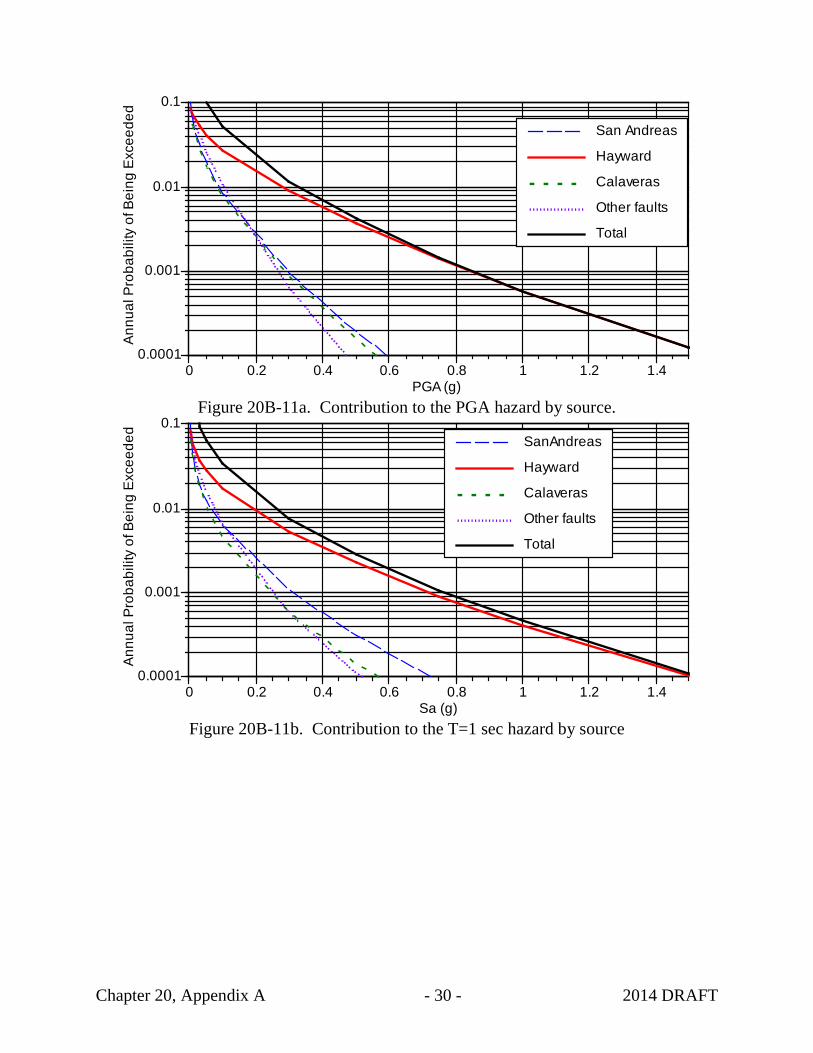
Chapter 20, Appendix A - 30 - 2014 DRAFT
Figure 20B-11a. Contribution to the PGA hazard by source.
Figure 20B-11b. Contribution to the T=1 sec hazard by source
0.0001
0.001
0.01
0.1
0 0.2 0.4 0.6 0.8 1 1.2 1.4
Ann
ual P
roba
bilit
y of
Bei
ng E
xcee
ded
PGA (g)
San Andreas
Hayward
Calaveras
Other faults
Total
0.0001
0.001
0.01
0.1
0 0.2 0.4 0.6 0.8 1 1.2 1.4
Ann
ual P
roba
bilit
y of
Bei
ng E
xcee
ded
Sa (g)
SanAndreas
Hayward
Calaveras
Other faults
Total

Chapter 20, Appendix A - 31 - 2014 DRAFT
Figure 20B-12a. Sensitivity of PGA hazard to attenuation relation.
Figure 20B-12b. Sensitivity of T=2 sec hazard to attenuation relation.
0.0001
0.001
0.01
0.1
0 0.5 1 1.5
Annu
al P
roba
bilit
y of
Bei
ng E
xcee
ded
Peak Acceleration (g)
Abrahamson & Silva
Chiou & Youngs
Boore & Atkinson
Campbell & Bozorgnia
Idriss
0.0001
0.001
0.01
0.1
0 0.5 1 1.5
Annu
al P
roba
bilit
y of
Bei
ng E
xcee
ded
Spectral Acceleration (g)
Abrahamson & Silva
Chiou & Youngs
Boore & Atkinson
Campbell & Bozorgnia
Idriss

Chapter 20, Appendix A - 32 - 2014 DRAFT
Figure 20B-13a. Uncertainty fractiles of the PGA hazard
Figure 20B-13b. Uncertainty fractiles of the T=2 sec hazard
0.0001
0.001
0.01
0.1
0 0.2 0.4 0.6 0.8 1 1.2 1.4 1.6 1.8 2
Prob
abili
ty o
f Bei
ng E
xcee
ded
Peak Acceleration (g)
5th
15th
50th
85th
95th
Mean
0.0001
0.001
0.01
0.1
0 0.2 0.4 0.6 0.8 1 1.2 1.4 1.6 1.8 2
Prob
abili
ty o
f Bei
ng E
xcee
ded
Spectral Acceleration (g)
5th
15th
50th
85th
95th
Mean

Chapter 20, Appendix A - 33 - 2014 DRAFT
Figure 20B-14. UHS and deterministic (MCE) spectra for the Hayward/Rodgers Creek source.
0
0.5
1
1.5
2
2.5
3
3.5
0.01 0.1 1 10
Spec
tral A
ccel
erat
ion
(g)
Period (sec)
500 Yr
1000 Yr
2000 Yr
5000 Yr
Hayward Median (M7.25)
Hayward 84th (M7.25)
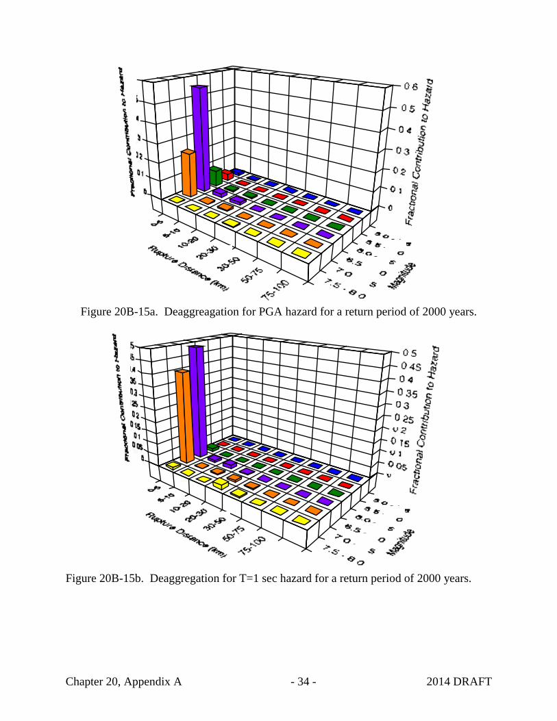
Chapter 20, Appendix A - 34 - 2014 DRAFT
Figure 20B-15a. Deaggreagation for PGA hazard for a return period of 2000 years.
Figure 20B-15b. Deaggregation for T=1 sec hazard for a return period of 2000 years.

Chapter 20, Appendix A - 35 - 2014 DRAFT
Figure 20B-16. Return period dependence of the Mean M, R, epsilon from the deaggreagation for PGA and T=1 sec
5
5.5
6
6.5
7
7.5
100 1000 10000
Mea
n M
agni
tude
Return Period (yrs)
PGA
T=1 sec
02
468
101214
100 1000 10000
Mea
n D
ista
nce
(km
)
Return Period (yrs)
PGA
T=1 sec
0
0.5
1
1.5
2
2.5
3
100 1000 10000
Mea
n E
psilo
n
Return Period (yrs)
PGA
T=1 sec

Chapter 20, Appendix A - 36 - 2014 DRAFT
Figure 20B-17 Expected spectra for scenario earthquakes for the UHS at T=0.2 and T=1.0 sec.
0
0.5
1
1.5
2
2.5
3
0.01 0.1 1 10
Spec
tral A
ccel
erat
ion
(g)
Period (sec)
2000 Yr UHS
Hayward (6.75)
Hayward (7.0)

Chapter 20, Appendix A - 37 - 2014 DRAFT
Figure 20B-18 Example of broadening the expected spectra for scenario earthquakes into a small set of design spectra.
0
0.5
1
1.5
2
2.5
3
0.01 0.1 1 10
2000 Yr UHS
Hayward (6.75)
Hayward (7.0)
Design Scenario 1
Design Scenario 2

Chapter 20, References - 1 - 2014 DRAFT
REFERENCES A primary reference is the Bureau of Reclamation and U.S. Army Corps of Engineers Best Practices, Chapter 6, Seismic Hazard Analysis (2/24/2009). This reference, last updated on September 6, 2012, can be found at the following website:
http://www.usbr.gov/ssle/damsafety/Risk/methodology.html It is not reprinted here. Abrahamson, N.A. (2000). “State of the practice of seismic hazard assessment.” Proceedings of GeoEng2000, Melbourne, Australia, vol.1, 659-685 Abrahamson, N. A. (2006). “Seismic Hazard Assessment: Problems with current practice and future developments.” First European Conference on Earthquake Engineering and Seismology, Geneva, Switzerland. Baker, J. W. (2008). An Introduction to Probabilistic Seismic Hazard Analysis (PSHA), Excerpt from a report originally written for the USNR. Baker, J. W. (2011). “Conditional Mean Spectrum: Tool for ground motion selection.” Journal of Structural Engineering, 137(3), 322-331. FEMA (2003). Federal Guidelines for Dam Safety: Glossary of Terms, Federal Emergency Management Agency, Washington D.C FERC (2006). Evaluation of Earthquake Ground Motions, prepared by I.M. Idriss and R.J. Archuleta, draft version 06.5. Federal Energy Regulatory Commission, Washington D.C Fraser, W. A., and Burns, R.G. (2004). “Evaluating the Conservatism of Deterministic Ground Motions using Probabilistic Seismic Hazard Analysis.” Association of Engineering Geologists, 2004 Annual Meeting, Dearborn, Michigan ICOLD (2010). Selecting Seismic Parameters for Large Dams, Bulletin 72, Committee on Seismic Aspects of Dam Design, ICOLD, Paris. Jack Benjamin & Associates, URS Corp., Geomatrix Consultants, Inc. and Shannon & Wilson, Inc. (2012). Final Report: Probabilistic Seismic Hazard Analyses Project for Mid-Columbia Dams, prepared for Public Utility Districts of Chelan, Douglas, and Grant Counties, February 2012.
Chapter 20, References - 2 - 2014 DRAFT
Luco, N., Ellingwood, B. R., Hamburger, R. O., Hooper, J. D., Kimball, J. K., and Kircher, C. A. (2007). “ Risk-Targeted versus Current Seismic Design Maps for the Coterminous United States.” SEAOC 2007 Convention Proceedings. Malhotra, P.K. (2006). “Seismic Risk and Design Loads.” Earthquake Spectra, Vol. 22, No. 1, pages 115-128, February 2006. McCann, M. W, Lord, D., Marshall, K., Mishalanie, D., Yow, G., and Christman, B. (2013). “Development of a Risk-Informed Approach to the Seismic Evaluation of Hydroprojects – Methodology” USSD Annual Conference, Phoenix, AZ Mejia, L, Gillon, M., Walker, J., and Newson, T. (2001). “Criteria for Developing Seismic Loads for the Safety Evaluation of Dams of Two New Zealand Owners” NZSOLD/ANCOLD 2001 Conference on Dams. McGuire, R.K. (1995). “Probabilistic seismic hazard analysis and design earthquakes: closing the loop.” Bulletin of Seismological Society of America 85(5), 1275-1284. PEER (2010). Technical Report for the PEER Ground Motion Database Web Application, Pacific Earthquake Engineering Research, Berkeley, California. Regan, P.J, and Boyer, D.D (2009). “Risk –Informed Decision Making in a Regulatory Context” ASDSO Annual Conference, Hollywood, FL, 43 pp. Regan, P.J, and Boyer, D.D (2008). “Beyond Black and White: Risk-Informed Decision Making in a Regulatory Environment.” USSD Annual Conference, Portland, OR, pp 269-278. Reiter, L. (1990). Earthquake hazard analysis: Issues and insights, Columbia University Press, New York. U.S. Department of Commerce (USDC) (2011). Selecting and Scaling Earthquake Ground Motions for Performing Response-History Analyses, NIST GCR 11-917-15, National Institute of Standards and Technology US Department of Interior, Bureau of Reclamation (2009). Risk Best Practices, Chapter 2, Seismic Hazard Analysis, February 24 US Department of Interior, Bureau of Reclamation and the U.S. Army Corps of Engineers (2012). Risk Best Practice, Chapter 6, Seismic Hazard Analysis, November 6

Chapter 20, References - 3 - 2014 DRAFT
US Department of Interior, US Geological Survey (USGS) (2008). Documentation for the 2008 Update of the United States National Seismic Hazard Maps, by M.D. Petersen et al. Open-File Report 2008-1128. US Department of Interior, USGS (2009). Implementation of the SSHAC Guidelines for Level 3 and 4 PSHAs—Experience Gained from Actual Applications, prepared by Thomas C. Hanks, Norm A. Abrahamson, David M. Boore, Kevin J. Coppersmith, and Nichole E. Knepprath. U.S. Geological Service US Nuclear Regulatory Commission (USNRC) (2012). Practical Implementation Guidelines for SSHAC Level 3 and 4 Hazard Studies, NUREG-2117, US Nuclear Regulatory Commission, Washington D.C USNRC (1997). Senior Seismic Hazard Analysis: Guidance on Uncertainty and Use of Experts, NUREG-6372, US Nuclear Regulatory Commission, Washington D.C USNRC (1997). Recommendations for Probabilistic Seismic Hazard Analysis: Guidance on Uncertainty and Use of Experts, prepared by Senior Seismic Hazard Analysis Committee (SSHAC) R. J. Budnitz (Chairman), G. Apostolakis, D. M. Boore, L. S. Cluff, K. J. Coppersmith, C. A. Cornell, P.A . Morris, NUREG/CR-6372, UCRL-ID- 122160 Vol. 1, U.S. Nuclear Regulatory Commission Wells, D., and Coppersmith, K. (1994). “New Empirical Relationships among Magnitude, Rupture Width, Rupture Area and Surface Displacement.” Bull. Seismol. Soc. Am. 98, no. 4, 1609-1632. Youngs, R., Arabasz, W.J., Anderson, R.E., Ramelli, A.R., Ake, J.P., Slemmons, D.B., McCalpin, J.P., Doser, D.I., Fridrich, C.J., Swan III, F.H., Rogers, A.M., Yount, J.C., Anderson, L.W., Smith, K.D., Bruhn, R.L., Knuepfer, P.L.K., Smith, R.B., dePolo, C.M., O’Leary, D.W., Coppersmith, K.J., Pezzopane, S.K., Schwatrz, D.P., Whitney, J.W., Olig, S.S., and Toro, G.R. (2003). “A Methodology for Probabilistic Fault Displacement Hazard Analysis (PFDHA).” Earthquake Spectra, Vol 19, Iss 1, February http://dx.doi.org/10.1193/1.1542891.
Youngs, R., and Coppersmith, K.J. (1985) “Implications of Fault Slip Rates and Earthquake Recurrence Models to Probabilistic Seismic Hazard Estimates”, Bull. Seismol. Soc. Am., Vol. 75, No. 4, 939-964, August.


