FFI RAPPORT

A COMPARISION OF MEASUREMENTS AND

PREDICTIONS OF HF GROUNDWAVE PROPAGATION

HVIDSTEN Knut Inge

FFI/RAPPORT-2005/01703

A COMPARISION OF MEASUREMENTS AND PREDICTIONS OF HF GROUNDWAVE PROPAGATION

HVIDSTEN Knut Inge

FFI/RAPPORT-2005/01703

FORSVARETS FORSKNINGSINSTITUTT Norwegian Defence Research Establishment P O Box 25, NO-2027 Kjeller, Norway

3

FORSVARETS FORSKNINGSINSTITUTT (FFI) UNCLASSIFIED Norwegian Defence Research Establishment _______________________________ P O BOX 25 SECURITY CLASSIFICATION OF THIS PAGE N0-2027 KJELLER, NORWAY (when data entered) REPORT DOCUMENTATION PAGE 1) PUBL/REPORT NUMBER 2) SECURITY CLASSIFICATION 3) NUMBER OF

FFI/RAPPORT-2005/01703 UNCLASSIFIED PAGES

1a) PROJECT REFERENCE 2a) DECLASSIFICATION/DOWNGRADING SCHEDULE 89 FFI II/822/912 - 4) TITLE

A COMPARISION OF MEASUREMENTS AND PREDICTIONS OF HF GROUNDWAVE PROPAGATION

5) NAMES OF AUTHOR(S) IN FULL (surname first)

HVIDSTEN Knut Inge

6) DISTRIBUTION STATEMENT

Approved for public release. Distribution unlimited. (Offentlig tilgjengelig)

7) INDEXING TERMS IN ENGLISH: IN NORWEGIAN:

a) ground wave a) jordbølge

b) HF b) HF

c) surface wave c) overflate-bølge

d) knife-edge loss d) kniv-egg tap

e) EM propagation e) EM bølgeutbredelse

THESAURUS REFERENCE:

8) ABSTRACT

The field-strength of HF groundwave was logged for 6 different locations in the south-eastern part of Norway. Results were compared to models that take terrain elevation and ground conductivity/permittivity as input parameters. Performance of models was analysed and on this basis, and a simple model was recommended. It was found that the terrain profile is important even for frequencies in the lower HF range for terrain typical of Norway. For land-based paths, ground electrical parameters are highly important, and further work on proper identification of these is recommended.

9) DATE AUTHORIZED BY POSITION

This page only 2005-04-10 Vidar S Andersen Director

ISBN 82-464-0958-1 UNCLASSIFIED

SECURITY CLASSIFICATION OF THIS PAGE (when data entered)

5

CONTENTS Page

1 INTRODUCTION 7

2 HF GROUNDWAVE PROPAGATION 8

2.1 Electrical parameters 8

2.2 Changes in electrical parameters 11

2.3 Formulating a model for HF ground-wave 14

2.4 Wave-tilt and attenuation method 16

2.5 Height-gain 17

3 IMPLEMENTED MODELS 19

3.1 Flat earth model 19

3.2 GRWAVE 20

3.3 Millington 20

3.4 Clearance angle 20

3.5 Bullington 21

3.6 Blomquist & Ladell 21

3.7 WAGSLAB 22

3.8 Functional testing 23

4 MEASUREMENT SETUP 27

4.1 Basic setup 27

4.2 Measurement equipment 28

4.3 Receiver sensitivity 29

4.4 Transmitter Effective Radiated Power measurements 31

4.5 Antenna diagrams and ground influence 33

4.6 Data logging 34

4.7 Sources of error 35

5 MATLAB PROCESSING 37

5.1 MATLAB environment 37

5.2 Estimating position/field-strength 38

6 MEASUREMENTS 40

6.1 Background 40

6.2 Locations 41

6.3 Noise 42

6

6.4 Spatial Fading 46

6.5 Measurements at each path 51 6.5.1 The Bjørkelangen path 51 6.5.2 Measurements at remaining paths 58 6.5.3 Characterising measurements using a wider range of models 63

7 CONCLUSION AND RECOMMODATIONS 66

References 67

APPENDIX

A ABBREVIATIONS AND ACRONYMS 70

B MAPS AND METEOROLOGICAL DATA 71

B.1 Digital elevation maps 71

B.2 N50 vector maps 71

B.3 Agriculture/forest productivity maps 71

B.4 Soil geology maps 71

B.5 Solid rock geology maps 71

C METEOROLOGY 72

D CALIBRATION DOCUMENTATION FROM NEMKO COMLAB 74

E CONVERTING SIGNAL VOLTAGE TO SIGNAL POWER CALIBRATION 75

F LIST OF EQUIPMENT 76

G SENSITIVITY TO CONDUCTIVITY AND PERMITTIVITY AT 0.3, 3 AND 30 MHZ 77

H MEASUREMENTS AND PREDICTIONS 78

7

A COMPARISION OF MEASUREMENTS AND PREDICTIONS OF HF GROUNDWAVE PROPAGATION

1 INTRODUCTION

Throughout the 20th century, electromagnetic (EM) groundwave propagation has been at the focus of researchers such as Sommerfeld (1), Norton (2) and Millington (3). A nice summary can be found in (4). The accurate prediction of groundwave field-strength/path-loss is crucial to different applications such as naval HF communications, HF radar and MF AM radio. Groundwave is usually considered the primary propagation mode (or secondary of importance) for earth-bound stations in the frequency range from tens of kHz (Low Frequency) to 30 MHz or more (into the VHF range) The aim of this work was to suggest a replacement or refinement of the groundwave propagation model used in the Norwegian forces joint frequency administration program (FEFAS). Special attention was given to groundwave propagation over rough land-paths thought to be representative of the terrain commonly found in inland Norway. A practical approach was chosen, performing measurements and comparing them with existing models. This research was funded by the Norwegian Defence Research Establishment (FFI). Chapter 2 contains a short summary of HF propagation basics and relevant parameters suitable for new readers, while Chapter 3 and 5 describe computer tools for modelling propagation and comparing measurements to predictions. Chapter 4 and 6 describe the setup and actual measurements conducted. Chapter 7 contain the findings and conclusions of this work The author would like to thank the following persons for good help with different parts of the project; Bjørn Solberg and Vivianne Jodalen for continual support and constructive critisism, Anders Johnsen and Martin Hassel Aaser for doing measurements as part of a bachelor thesis, Jostein Sander and Audun Simonsen for help with the field measurements (as well as Audun doing some MATLAB coding and Fortran compilation), Knut Stokke, Bodil Hvesser Farsund and Walther Åsen for input to this work, Ørnulf Kandola for help on GPS systems as well as Steinar Svalstad and Frode Tørres at Hærens Samband Utdanning og Kompetansesenter (HSBUKS) for the transmitter vehicle.

8

2 HF GROUNDWAVE PROPAGATION

This work considers only propagation in the HF frequency range (3 MHz to 30 MHz), and only groundwave propagation. Ionospheric propagation, best known for its capability of communication at great distances, is not considered. The theory behind groundwave propagation was previously considered in (5). Only a short summary essential for the understanding of the measurements will be given here. Earth-bound radio propagation is commonly simplified from 3 dimensions into a 2-D plane defined by a source (transmitting radio), receiver, and an angle normal to the ground. This is valid as long as the variation in the third axis is neglectable, or equivalently, that the energy spreads as a single point on a sphere of infinite power density from the transmitter to the receiver with no interaction outside the 2-D slice. Using geometrical optics from higher frequency prediction models, one would model the path as a set of horizontal reflectors and vertical absorbing knife edges. Due to the long wavelengths in the HF band (10-100m) one would expect less loss from obstacles. Also, since HF terminals are usually close to the ground in terms of wavelength, one would expect a strong phase-reversed ground-reflection that would effectively cancel the direct path signal and leave no signal at the receiver. Early experimenters were puzzled by the ability to transmit over large distances, even though the wavelengths were large, and antennas were situated on the ground. Zenneck (6) were the first to include a “surface wave” in the analysis of Maxwell’s equations for a vertically polarized plane wave travelling along the interface between air and an infinite plane of finite conductivity. Later, Sommerfeld (1) and Norton (2) provided different solutions to the wave equation that extended the idealised case to a vertical electric dipole located close to a spherical, conducting earth. The “surface wave” has been described as a “correction term” that bridge the gap between geometrical optics and Maxwell`s equations (7).

2.1 Electrical parameters

The surface wave can be seen as EM energy close to the air-earth interface, guided by diffraction to follow the curved earth. The horizontally polarized surface wave is heavily attenuated and usually not of interest, while the vertically polarized wave can travel great distances depending on the ground-losses.

Figure 2.1 Conceptual figure of energy-flow for surface wave, from (7)

9

Figure 2.1 visualizes this as the flow of energy traveling above the air/ground interface beyond some distance from the transmitter, with a continual loss of energy to the ground. The receivers at M1 and M2 then see an additional loss to the local ground preceding each. Important parameters for determining ground-losses are the electrical characteristics of the earth:

• Magnetic permeability, normally assumed to be equal to that of vacuum

μ = μ0 = 4*π*10-7 H/m

• Electric permittivity,

ε = εr*ε0

ε0 = 8.85*10-12 F/m

• Electric conductivity,

σ [S/m] εr and σ are functions of the ground type. Sea-water has a high conductivity and permittivity (in the region of 5 S/m and 80, respectively), explaining the good conditions found for groundwave communication at sea, while ground has a much lower set of values (from 10-5 to 2*10-1 and 3 to 60, respectively). The conductivity as well as permittivity of water is found to be a function of the degree of impurities (salt, ions) and temperature (8). While sea-water is highly conductive, fresh water shows a medium conductivity depending on purity, while distilled water and ice has very low conductivity (below 10-4 S/m in the HF range). Ground conductivity is primarily a function of the moisture content and differences between soil-types have been traced to differences in capability of storing moisture. Figure 2.2 shows a prediction of field strength by GRWAVE at 10 MHz and 10 km.

10

Figure 2.2 Field strength calculated for varying electrical conditions at 10 MHz, 10km

Figure 2.3 Field strength at 10 km for different frequencies and ground types

In the x- and y-axis, conductivity and permittivity are stepped through realistic values showing the sensitivity to both. Points are inserted at the approximate positions recommended in (8). For water the main concern is conductivity, as variations along the permittivity axis are small. The opposite applies for ground where permittivity is most important, especially at the lower frequencies. Further insight can be gained by inspecting Figure 2.3, where the points from Figure 2.2 are recorded for a number of frequencies inside and outside the HF band. Field strength decreases as frequency increases. Further, in the limit of zero frequency, the sensitivity to sea salinity decreases, as does the difference between best (sea water) and worst (very dry ground) conditions. As the frequency increases, the dependency on conductivity decreases until we

11

have a situation known from VHF, where permittivity is most important and the attenuation is relatively high. An empirical equation relating conductivity to permittivity is described in (9). A program modelling a smooth spherical, homogenous earth with a realistic atmosphere was made by Rotheram (10) and used as basis for the curves presented in (11), an example is provided in Figure 2.4. Within its validity (a single set of ground constants and no terrain obstacles) it allows flexibility in input parameters and good correspondence with measurements.

Figure 2.4 Example of ITU-R P.368-7 propagation curves for 10kHz-30MHz

2.2 Changes in electrical parameters

So far, we have considered antennas on top of a uniform conducting earth. In practice there are changes both horizontally and vertically, complicating the models and modelling. Vertical changes can happen when there is a thin layer of low conductivity/permittivity on top of a thick layer of better conductivity, such as ice on seawater or dry sand on moist clay. The analytic solution to such problems is to use the skin-depth, defined as the depth where the field strength is attenuated to 1/e times its value at the surface. From the figure in (8), we see that skin depth typically decreases with increasing frequency and with increasing conductivity/permittivity. For sea-water it is between 4 and 15 cm in the HF range. For other ground types except ice, it is between 100m and 2m. This means that for high frequencies and good ground, it may make sense to measure/model only the top layer, as the wave has little interaction with lower layers. For lower frequencies

12

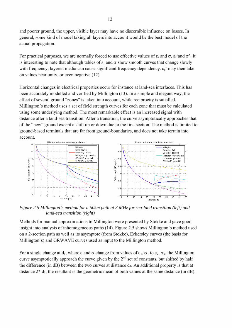
and poorer ground, the upper, visible layer may have no discernible influence on losses. In general, some kind of model taking all layers into account would be the best model of the actual propagation. For practical purposes, we are normally forced to use effective values of εr and σ, εr‘and σ’. It is interesting to note that although tables of εr and σ show smooth curves that change slowly with frequency, layered media can cause significant frequency dependency. εr‘ may then take on values near unity, or even negative (12). Horizontal changes in electrical properties occur for instance at land-sea interfaces. This has been accurately modelled and verified by Millington (13). In a simple and elegant way, the effect of several ground “zones” is taken into account, while reciprocity is satisfied. Millington’s method uses a set of field strength curves for each zone that must be calculated using some underlying method. The most remarkable effect is an increased signal with distance after a land-sea transition. After a transition, the curve asymptotically approaches that of the “new” ground except a shift up or down due to the first section. The method is limited to ground-based terminals that are far from ground-boundaries, and does not take terrain into account.

Figure 2.5 Millington`s method for a 50km path at 3 MHz for sea-land transition (left) and land-sea transition (right)

Methods for manual approximations to Millington were presented by Stokke and gave good insight into analysis of inhomogeneous paths (14). Figure 2.5 shows Millington`s method used on a 2-section path as well as its asymptote (from Stokke), Eckersley curves (the basis for Millington`s) and GRWAVE curves used as input to the Millington method. For a single change at d1, where ε and σ change from values of ε1, σ1 to ε2, σ2, the Millington curve asymptotically approach the curve given by the 2nd set of constants, but shifted by half the difference (in dB) between the two curves at distance d1. An additional property is that at distance 2* d1, the resultant is the geometric mean of both values at the same distance (in dB).

13

Figure 2.6 Millingtons method used for 50 km "wetground" at 3 MHz and inserted zones of:

top left: 4km sea water, bottom left: 40 km of sea water, top right: 4 km of "poor ground", bottom right: 40 km of "poor ground"

In Figure 2.6, we have plotted predictions for some extreme cases of inserted zones into a 50 km path of wet ground at 3 MHz. The upper row is for a 4 km insertion, while the lower is a 40 km insertion. The left column shows an insertion of very good ground (sea water), while the right column is the opposite, very dry ground. As can be seen from the figure, while a change in ground constants can cause a remarkable change “locally” (inside the inserted zone of differing properties), once past it, the field strength rapidly approach that of the global curve. The exception to this is an inserted zone that is sufficiently long and of different properties to give an appreciable shift upwards or downwards, typical of mixed sea-land paths. For the figure at bottom left, the inserted section of sea water cause an appreciable rise in levels even past the zone of sea water. By inspecting the “Millington approximation” in light blue, we see that the asymptote is some 10 dB over the field that would be predicted had there been no sea section. For the case of HF groundwave propagation over land, the picture at bottom right is more relevant. Here, we see that even a long section of quite different properties makes little to no difference once the receiver is out of that zone. This is a different way of formulating that the ground found at transmitter and receiver should matter most, used in parts of DETVAG-901: 1 A program developed by FOI for propagation modelling for a wide range of frequencies, including the HF band (15). Of special interest here because it uses the Blomquist & Ladell formula for integrating diffraction and smooth earth losses.

14

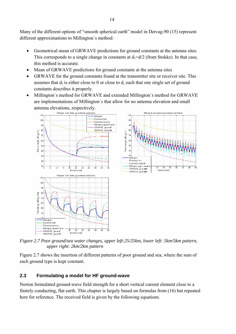
Many of the different options of “smooth spherical earth” model in Detvag-90 (15) represent different approximations to Millington`s method:

• Geometrical mean of GRWAVE predictions for ground constants at the antenna sites. This corresponds to a single change in constants at d1=d/2 (from Stokke). In that case, this method is accurate.

• Mean of GRWAVE predictions for ground constants at the antenna sites • GRWAVE for the ground constants found at the transmitter site or receiver site. This

assumes that d1 is either close to 0 or close to d, such that one single set of ground constants describes it properly.

• Millington`s method for GRWAVE and extended Millington`s method for GRWAVE are implementations of Millington`s that allow for no antenna elevation and small antenna elevations, respectively.

Figure 2.7 Poor ground/sea water changes, upper left:25/25km, lower left: 5km/5km pattern, upper right: 2km/2km pattern

Figure 2.7 shows the insertion of different patterns of poor ground and sea, where the sum of each ground type is kept constant.

2.3 Formulating a model for HF ground-wave

Norton formulated ground-wave field strength for a short vertical current element close to a finitely conducting, flat earth. This chapter is largely based on formulas from (16) but repeated here for reference. The received field is given by the following equations.

15

Figure 2.8 Geometry used in formulating Norton ground-wave (16)

1 2

2

1 2

2 21 2

1 2

2 4 22

2

1 1 2 21 2

222 2 2 2 2

2 2 2

1 130 cos cos

1(1 )(1 cos )

1 130 ( )cos( ) ( )cos( )

coscos( )(1 ) 1 cos 1 (1 cos )2 2

jkr jkrz v

jkrv

jkr jkrv

v

E j kIdl e R er r

R u u F er

E j kIdl sin e sin R er r

uR u u u

ρ

ψ ψ

ψ

ψ ψ ψ ψ

ψψ ψ ψ

− −

−

− −

⎡⎧ ⎫= + +⎨ ⎬⎢

⎩ ⎭⎣⎤

− − + ⎥⎦

⎡= − + −⎢

⎣

− − − − + 2

2

1 2

1

ψ andψ from figure

12

dipole momentplane-wave Fresnel vertical polarised reflection coefficientattenuation function

jkr

v

F er

j

k

IdlRF

πλ

− ⎤⎧ ⎫⎨ ⎬ ⎥⎩ ⎭ ⎦

= −

=

==

=

16

2 2 22 2

2

2

4

0

1 { ( )}

2 (1 cos )(1 )

1( )

1.8 10

w

v

r

MHz

F j we erfc j w

j kr u uwR

ujx

xf

π

ψ

εσ σ

ωε

−⎡ ⎤= −⎣ ⎦− −

=−

=−

= = ×

This formulation may be extended to a spherical earth, and several terms may be ignored or simplified for practical situations. For HF ground-wave propagation (where terminals usually are close to the ground in terms of wavelength due to the long wavelengths), the prime interest is usually the Ez term. It may be simplified by recognizing that the Fresnel reflection coefficient approach –1 in the limit of “low” terminals (gracing incidence), regardless of ground electrical parameters. Therefore, the first two terms of Ez tend to cancel, and we are left with

2 4 160 (1 ) jkrzE j kIdl u u F e

r−= − +

We can further simplify this expression to: 300| | | |z

mVE F Pr m

⎡ ⎤= ⎢ ⎥⎣ ⎦

This is assuming that the (1-u2+u4)-factor tend to one, P being total radiated power from a Hertzian-dipole current element in kW and r representing path length in km. F then is the “unknown” that is essential for predicting field strength at a point due to a known source.

2.4 Wave-tilt and attenuation method

The formulas presented in 2.3 can also be used to estimate the electrical characteristics of the ground. One such method is wave-tilt (12), in which the forward tilt angle of the predominantly vertically polarized wave front is measured in some way. This can be accomplished by rotating a wire antenna from vertical to horizontal orientation. By recording the angle of maximum, as well as ratio between maximum and minimum, the complex dielectric permittivity (containing both εr and σ) can be found.

17

Figure 2.9 Conceptual figure showing propagation and wavetilt, from(17)

Figure 2.9 illustrates wave-tilt appears as a downward tilt close to the ground. As the frequency is increased and/or ground parameters get worse, ground losses increase and the

wave-front is more tilted. One problem with the wave-tilt method is that the ratio zEEρ

can be

very large. This leads to difficulties in determining the precise ratio. The attenuation method is an alternative method of estimating ground parameters using Millingtons method in reverse (29). By “adjusting” ground parameters manually or using a computer program until a Millington prediction fits, estimates of ground parameters can be found. As the wave front at each point contains the history of every preceding point, the method has limited spatial resolution. If an abrupt transition in ground occurs, the receiver has to traverse some distance into the second ground type. This method assumes a smooth earth. In other words, it would be expected to deliver better results for lower frequencies than higher. A practical upper limit of 8-10 MHz is indicated in (29).

2.5 Height-gain

According to the Federal Standard 1037C, height gain is defined as: height gain: For a given propagation mode of an electromagnetic wave, the ratio of the field strength at a specified height to the field strength at the surface of the Earth.

ionosphere

Wavefront over ground Wavefront

over ideal conductor

18

For HF ground wave propagation, we typically see a strong, positive height-gain for realistic elevation. As the terminal is further elevated, the importance of surface wave is diminished, and we are left with a direct and reflected wave summation. This is reflected by the GRWAVE switching to a geometric propagation model once elevation exceeds a threshold.

19

3 IMPLEMENTED MODELS

To be able to compare measurements with predictions, various models were implemented either directly in MATLAB, or accessed externally through a MATLAB function. As the type and format of input variables and output predictions vary, they were all accessed through a MATLAB function called models. The rest of this chapter describes in some detail the implementation of each model.

Figure 3.1 Models implemented in MATLAB

Although the sub modules allowed predictions along a radial or terrain profile, only a single point was calculated, while an external loop swept models through the desired points. From a computation standpoint this is clearly inefficient. Some kind of 2-dimensional area coverage grid, interpolated to find exact values would clearly be better. However, this would cause additional implementation complexity, as well as the uncertainty of interpolation.

3.1 Flat earth model

A simple “baseline” model was desirable. The formulas presented in (16), derived from (2) were implemented for this purpose. Input parameters are:

• Conductivity • Permittivity • Wavelength • Distance

20

• Transmitter power • Frequency

In addition to predicting the vertical electrical field strength, a value for lossless ground is provided (assuming zero antenna elevation). This model is basically limited by the distance d=80/sqrt(FMHz) [km], where the flat-earth approximation fails.

3.2 GRWAVE

The FORTRAN program GRWAVE is available compiled for the windows platform from the ITU (18). A MATLAB function was implemented, giving access to relevant input parameters as well as re-formatting the output text file to a more convenient set of numeric vectors. GRWAVE is considered valid for any geometry and distance as long as the earth can be considered smooth, spherical and homogeneous.

3.3 Millington

The implementation of Millington’s method builds upon GRWAVE to provide multiple zones of electrical parameters for ground-based terminals. The distance between transmitter and receiver may be any value, but transitions in ground parameters may only occur at integer kilometer values. This is thought to be sufficient as long as the terminals are not placed close to a ground transition, in which Millington’s method is not suited. As Millington’s method use Eckersley’s method forwards and backwards, these are also provided in the function output. The asymptotic value described in (14) is provided as well.

3.4 Clearance angle

The use of clearance angle for HF groundwave was defined in previous papers (5) and (19). A correction to any smooth earth model (for instance GRWAVE) for rough terrain was obtained by evaluating the obstruction of horizon. Earth flattening is used because no correction is wanted in the limit of smooth earth; we are assuming that smooth earth models give correct predictions as terrain variation approach zero. The parameter linking “Clearance angle” to additional terrain loss was found experimentally in (5) to be close to 1 for profiles considered. This means an additional loss of 1 dB for every degree of horizon obstruction for both transmitter and receiver.

21

Figure 3.2 Comparing Clearance Angle losses to Bullington method for diffraction losses

(based on Fresnel).

When comparing CLA to diffraction losses predicted using Bullington diffraction, we note that CLA is frequency independent and that up until gracing angle (half-space), it is equal to zero.

3.5 Bullington

Bullington’s method for calculating diffraction losses closely resembles the “Clearance angle” method outlined above, while being more physically based. It is also easily implemented compared to more elaborate diffraction methods. It can be argued that error margins are a lot bigger when predicting HF groundwave propagation as compared to VHF or higher frequencies. Due to this, the improved accuracy of alternative multiple knife-edge methods may not be that important.

3.6 Blomquist & Ladell

The “Blomquist & Ladell” method is an empirical model to combine the losses from a smooth spherical earth with those of a multiple knife edge model. In the limit of low frequencies it degenerates to the smooth earth loss, while in the limit of high frequencies, it degenerates to knife edge loss. Both properties are physically sound. It also assures that the resultant loss is at least as large as either smooth earth or knife edge loss alone. In the 1974 paper (20), it is strictly recommended for frequencies above 30MHz, but in correspondence with Aerotech Telub it was suggested used for lower frequencies as well.

22

Ltot = Lfree - sqrt(FB2 + FEP

2) Lfree is the basic free space transmission loss F is a propagation factor, or the difference between free space loss and total loss FB is the smooth earth propagation factor FEP is the diffraction propagation factor All values are in dB

Figure 3.3 Combining smooth earth and knife edge loss from (20)

For our frequencies the loss calculated is close to that of the smooth earth model alone. Diffraction model losses are overpowered by smooth earth losses as the wavelength enters the HF range. For knife edge losses, the results from the Bullington diffraction model is used. Although Detvag90 use better diffraction models, in our scenario this would make neglectable differences for the wavelengths at hand.

3.7 WAGSLAB

FORTRAN code was retrieved from original WAGSLAB papers (21), extending on code and principles from WAGNER (28), and compiled for windows. The code allows for a large number of parameters to be set, and the MATLAB function wagslab3_wrap gives access to all inputs and outputs. However, only a limited subset will actually be used in this report. Essential parameters include:

• Distance • Frequency • Elevation • Up to 50 terrain profile points

23

• Up to 50 ground electrical characteristics zones with possibility for two vertical layers (slabs)

For cases where the input terrain profile was longer than the maximum of 50 points, special care had to be taken. First, dividing the profile into 50 equal length sections was tried, where each section got its value from the mean of original samples within that range. As this caused problems in the vicinity of receiver and transmitter, another method was found to give better results. Within each section, the elevation and position was selected as the profile point that gave highest diffraction losses in the Bullington prediction. This results in a “maximum envelope” kind of function that would likely give good results in a multi knife-edge method.

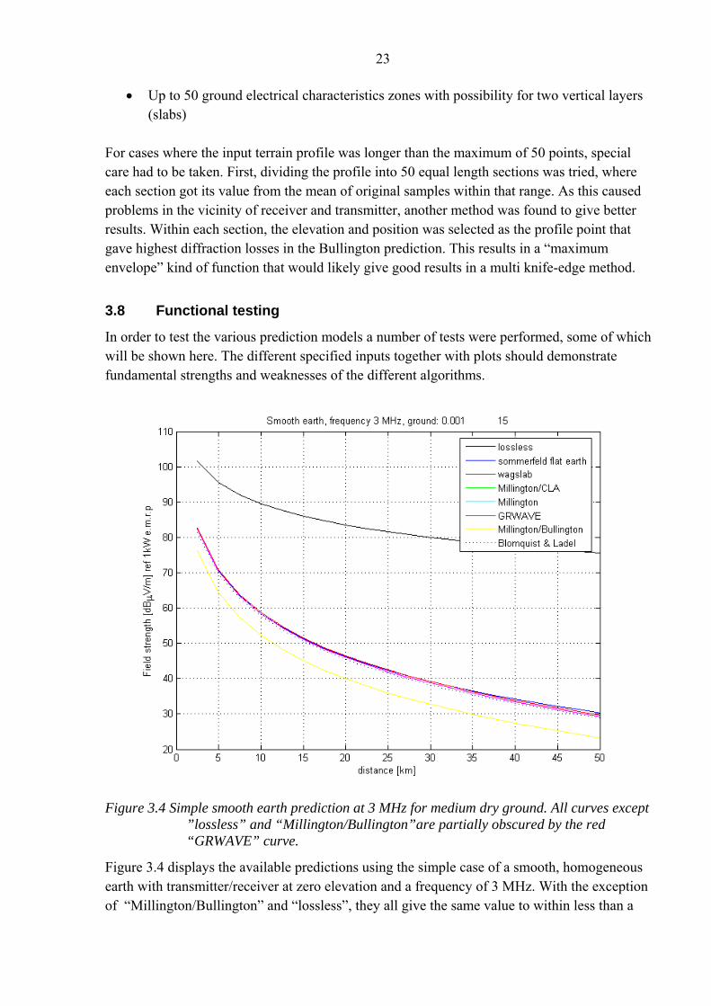
3.8 Functional testing

In order to test the various prediction models a number of tests were performed, some of which will be shown here. The different specified inputs together with plots should demonstrate fundamental strengths and weaknesses of the different algorithms.

Figure 3.4 Simple smooth earth prediction at 3 MHz for medium dry ground. All curves except

”lossless” and “Millington/Bullington”are partially obscured by the red “GRWAVE” curve.

Figure 3.4 displays the available predictions using the simple case of a smooth, homogeneous earth with transmitter/receiver at zero elevation and a frequency of 3 MHz. With the exception of “Millington/Bullington” and “lossless”, they all give the same value to within less than a

24

dB. In the case of “Millington/Bullington”, groundwave and diffraction losses are combined in a way that results in overly pessimistic predictions for a smooth/flat earth. As it is well known that ground wave losses are high over land at this frequency (11), it should come as no surprise that “lossless” is markedly different from other predictions.

Figure 3.5 1MHz, 150km, sea-water

In Figure 3.5, a completely different picture is seen when the frequency is lowered to 1 MHz and a long-distance sea-water path of 150 km is simulated. Field strength is close to the ideal, lossless case up to 50km. This corresponds well with theory, suggesting that flat-earth models (“lossless”, “sommerfeld flat earth”) are incorrect beyond 80 km for this case. Interestingly, the “Blomquist & Ladel” model, clearly used outside its original scope, is more or less identical to the “Millington/Bullington” method, as surface wave losses are small, leading to an increased relative influence of diffraction losses.

25

Figure 3.6 Combination of terrain profile featuring a triangular wedge as well as changes in

ground constants

Figure 3.7 Predictions for terrain profile depicted above

Figure 3.6 and Figure 3.7 respectively contains a more complex physical situation, and predictions using it. Strengths and weaknesses about the models can be learned from this figure. We see that “Sommerfeld flat earth” and “GRWAVE” are smooth. They behave as if no transitions occurred in ground constants and the wegde was not there. “Millington” and models extending Millington has a marked drop beyond 5km due to worse ground constants. So does the “wagslab” model. Diffraction-based models (“Millington/CLA”, “Millington/Bullington” and to a lesser extent “Blomquist & Ladel”) have a drop in field strength behind the wedge. But only “wagslab” has a discernible rise in field strength as the receiver is climbing up the “lit” side of the wedge. Actually, models based on the “Bullington”

26

diffraction also feature a similar signal gain, but due to the handling of “knife edge” for line of sight, it is miniscule.

27

4 MEASUREMENT SETUP

4.1 Basic setup

It was desirable to relate field strength to terrain position for a HF transmitter and receiver. To accomplish this, a mobile HF transmitter as well as receiver vehicle was used. Ideally, one would want a transmitter of known output power, well-defined directivity (preferably an omni-directional antenna diagram), and high stability in amplitude and frequency. Similarly, the receiver should have a calibrated sensitivity relating radio signal levels to field strength at the antenna as well as low internal noise. The need for mobile stations means constraints on grounding, physical size and power consumption, among other things. Practical considerations also lead to the use of field equipment instead of laboratory equipment in the transmitter and parts of the receiver. Four frequencies spread over the HF band were selected from a set of frequencies allowed by the Norwegian telecom authorities (Post -og Teletilsynet):

Table 4.1 Frequencies used for measurements

Frequency [MHz] 3.172 9.2875 16.041 24.7815 From now on, these frequencies will be referred to as 3, 9, 16 and 25 MHz unless otherwise specified. In hindsight it seems likely that a logarithmic rather than this near linear distribution of measurement frequencies would have provided more information about the channel for a given number of frequencies. This is evident in the “gap” between 3 and 9 MHz that will be shown later. Measurements of receiver and transmitter characteristics were carried out on a field/farmland, Jølsen gård near FFI, Kjeller. Care was taken to find a spot with minimal potential reflectors (power/telephone lines, buildings etc) and flat landscape with assumed small variation in ground constants. See Figure 4.1.

28

Figure 4.1 Examples of calibration measurement site

Some transmitter measurements mentioned in this chapter were done with a different receiver antenna, calibrated separately for earlier measurements (5). Care was taken so this should not be a source of error.

4.2 Measurement equipment

Figure 4.2 Measurement equipment

An important feature of the used setup (Figure 4.2) is an active receiver antenna of about 60 cm, allowing measurements to be conducted while the vehicle is in motion. To be able to relate

29

field strength to position, a GPS receiver was connected to the PC, logging positions at regular intervals. The transmitter is a standard equipped Siemens HF-3 mobile station with a 6 meter vertical monopole and with provisions to key CW transmission. It was possible to switch transmitter power between 1, 20, 100 and 400 Watt rated output power, and the receiver had a ~25 dB signal amplifier that could be inserted when needed. Both transmitter power and the use of receiver signal amplifier was calibrated relative to a common reference. This way, certain calibration measurements could be carried out at relatively small distances without overloading the receiver, while main measurements could be accomplished with optimal noise performance. As a general rule, 400W and receiver signal amplifier were the only setting used for main measurements to follow in later chapters2.

4.3 Receiver sensitivity

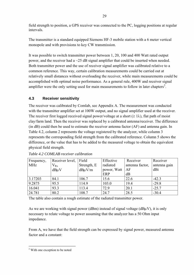
The receiver was calibrated by Comlab, see Appendix A. The measurement was conducted with the transmitter amplifier set at 100W output, and no signal amplifier used at the receiver. The receiver first logged received signal power/voltage at a short (≥ 1λ), flat path of moist clay/farm land. Then the receiver was replaced by a calibrated antenna/receiver. The difference (in dB) could then be used to estimate the receiver antenna factor (AF) and antenna gain. In Table 4.2, column 2 represents the voltage registered by the analyzer, while column 3 represents the corresponding field strength from the calibrated reference. Column 5 shows the difference, or the value that has to be added to the measured voltage to obtain the equivalent physical field strength.

Table 4.2 COMLAB receiver calibration

Frequency, MHz

Receiver level, VRx dBμV

Field Strength, E dBμV/m

Effective radiated power, Watt ERP

Receiver antenna factor, AF dB

Receiver antenna gain dBi

3.17203 84.1 106.7 15.6 22.6 -42.3 9.2875 95.5 114.9 103.0 19.4 -29.8 16.041 93.3 113.4 72.9 20.1 -25.7 24.781 80.2 108.7 24.7 28.5 -30.4 The table also contain a rough estimate of the radiated transmitter power. As we are working with signal power (dBm) instead of signal voltage (dBμV), it is only necessary to relate voltage to power assuming that the analyzer has a 50 Ohm input impedance. From A, we have that the field strength can be expressed by signal power, measured antenna factor and a constant: 2 With one exception to be noted

30

E = VRx,dBμV + AF = PRx dBm + kf [dBμV/m] Where : kf = 107 + AF is the value that we have to add to logged signal power. f, MHz PRx

dBm Field strength, E dBμV/m

’kf’, dB

3.17203 -22.9 106.7 129.6 9.2875 -11.5 114.9 126.47 16.041 -13.7 113.4 127.1 24.781 -26.8 108.7 135.5 After the calibration measurement, it was found that some changes were necessary to be able to measure at larger distances. In cases when the signal path gain is different from that of the calibration, kf is adjusted accordingly. For this purpose, the radiated transmitter output power were measured and related to that at 100W rated, and the gain of using signal amplifier in the receiver circuit were compared to using no amplifier.

Table 4.3 Receiver signal amplifier gain as a function of frequency

Frequency, MHz

AmpRx gain(dB)

3.17203 27.00 9.2875 27.33 16.041 26.67 24.781 26.84

Table 4.4 Power amplifier gain relative to that at "100W"

Switch [W] F [MHz] 1 20 100 400

3.17203 -25.67 -8.67 0 6

9.2875 -24.83 -8 0 5.17

16.041 -24.5 -9.17 0 4.83

24.781 -22.16 -9 0 7

Due to this, the transmitting frequency f at a power P when using the signal amplifier will be given by: E = PRx dBm + kf = PRx dBm + AF(f) + 107 – Pa(p,f) – Ps(f) [dBμV/m]

31

Where Pa and Ps can be found in Table 4.3 and

Table 4.4, AF is listed in Table 4.2 and PRx dBm is the measured signal to be read off the signal analyzer (log).

4.4 Transmitter Effective Radiated Power measurements

Basic antenna theory as well as COMLAB estimates indicates that a 6 m monopole is a difficult load at wavelengths up to 100 m. An antenna tuner can counter the load problem, however tuner losses increase as it has to counter the large antenna capacitance of a short monopole with an equally large inductance. Reading real radiated output power with a power meter is impossible, as there is no way to resolve the series connection of radiation resistance and ohmic losses in antenna and feeder cable. An error of some dB would shift the measured curves. Stokke (22) describes a concept for estimating the EMRP (Effective Monopole Radiated Power) using cymomotive force: c.m.f. = E*r Where E is field strength and r is distance. For a short monopole of P = 1kW on a perfectly conducting ground plane we have: c.m.f. = E*r = (300/r)*r = 300V Or a constant value that could be measured and used for EMRP estimation: EMRP = (c.m.f./300)^2 [kW] Due to finitely conducting ground, some decrease in c.m.f. with distance is expected. Also, changes in conductivity would cause variations. To get a good power estimate, Stokke suggests measuring along a radial from ~1λ (to avoid near-field effects) to a number of λs (15λ is mentioned), and fitting a line along the radial measurements into the transmitter. The value at 0 then should be used to estimate transmitter EMRP. In the remainder of this report, it is assumed that the losses in antenna tuner are not dependent on ground conditions. Due to this a single estimate of output power can be used for every location. One might argue that the transmitter tuner sees less radiation resistance and more capacitance for poor ground, and therefore introduce more non-ideal Ohmic losses. However, it is assumed that this effect is neglibible for the range of ground types and the precision considered here.

32

Figure 4.3 Cymomotive force and EMRP measurements. Note that a different, passive receiver

antenna was used, so calibrations in section 4.3 does not apply

Figure 4.3 shows measurements and calculations using cymomotive force to estimate output power. Both 9 and 16 MHz are reasonably close to rated power (-0.5 and +1dB, respectively). At 3 MHz and 24 MHz, however, the power is estimated at –6.4 and –13.1dB. The discrepancy at 3 MHz was expected due to the long wavelength. One possible reason for the error at higher frequencies may be that the antenna tuner is more efficient at capacitive (low frequency) than inductive (high frequency) loads.

33

4.5 Antenna diagrams and ground influence

Although single vertical radiators should have an omni-directional antenna diagram, the combination of antenna and vehicle might not. Some simple field measurements were carried out to investigate this, as well as effects of counterpoise and earth rod. For these measurements, the vehicle/counterpoise was rotated around the axis of the antenna, while received signal power was logged. As the path and every other parameter were left unchanged, any variation observed should be an estimate of the antenna diagram.

Figure 4.4 Receiver active antenna (left) and transmitter (right) measurements obtained by rotating the vehicle at 8 different angles. Normalised to 0 dB. Note different scales.

Figure 4.4 shows that the transmitter is circularly symmetric to within +/- 1dB for all frequencies considered. However the active receiver antenna has a 5-6 dB variation for the highest frequency. This was because of an asymmetric placement and insufficient grounding of the vehicle roof.

Figure 4.5 Counterpoise gain compared to no counterpoise(left) and passive receiver antenna (right) measurements obtained by rotating the counterpoise/vehicle respectively at 8 different angles. Normalised to 0dB(right)

34

Figure 4.5 shows that the counterpoise only has influence at 3 MHz, where it serves to increase output from 0.5 to 2 dB, especially along and opposite to the counterpoise. As this leads to a more asymmetric diagram and only a modest output improvement at the cost of more complex planning, no counterpoise was used in the further measurements. The passive receiver antenna showed an improved omni-directionality compared to the active one. Due to its length, it was not practical for continuous measurements while moving, and not used for further measurements. Measurements with and without transmitter earth-rod showed no difference at all, and it was used for all other measurements for safety reasons.

4.6 Data logging

Both analyzer and GPS logs are time stamped. The GPS logs each position with the corresponding time, typically every one or two seconds, while the analyzer software uses the local PC clock as a reference. A function in the GPS/NMEA logger allowed automatic adjustement of the PC clock, such that analyzer and GPS data have a common reference (GPS time). Start Logfile 07/08/04 12:26:58 ///////////////////////////////////// Spectrum Analyzer settings: ///////////////////////////////////// Aunits: DBM Cf: 9.28750E6 Rb: 1.00E2 Rl: -10.00 Sp: 0 St: 1.50E1 Vb: 1.00E2 Lg: 10 Start logging data ___________________ Time: 8270655 (binary data…) Time: 8285850 (binary data…) …

$GPGGA,125628.099,5959.4433,N,01149.3583,E,1,08,01.0,00240.9,M,36.2,M,,*67 $GPGSA,A,3,16,,24,01,10,27,17,,,08,13,,02.2,01.0,01.9*03 $GPGSV,3,1,11,16,21,036,34,24,38,243,36,01,12,084,32,10,36,297,38*7C $GPGSV,3,2,11,27,57,170,28,17,39,290,40,06,09,328,,04,17,206,*70 $GPGSV,3,3,11,08,30,194,29,13,60,092,32,33,07,207,*49 $GPRMC,125628.099,A,5959.4433,N,01149.3583,E,000.0,098.7,080704,001.4,E*6A $GPGGA,125629.099,5959.4433,N,01149.3583,E,1,08,01.0,00240.9,M,36.2,M,,*66 $GPGSA,A,3,16,,24,01,10,27,17,,,08,13,,02.2,01.0,01.9*03 $GPGSV,3,1,11,16,21,036,34,24,38,243,36,01,12,084,32,10,36,297,38*7C $GPGSV,3,2,11,27,57,170,28,17,39,290,40,06,09,328,,04,17,206,*70 $GPGSV,3,3,11,08,30,194,28,13,60,092,32,33,07,207,*48 $GPRMC,125629.099,A,5959.4433,N,01149.3583,E,000.0,098.7,080704,001.4,E*6B

Figure 4.6 Analyzer log file format(left)and logged standard NMEA format GPS data (right)

In Figure 4.6 , short examples of file formats used for logs are showed. To the left, header and two time slots of data are shown (actual binary containing exactly 601 samples not shown). The header contains information about analyzer settings and time (absolute time is polled from the computer clock), and every slot of data has a time-stamped offset in milliseconds. The

35

difference in time between slot[n] and slot[n+1] corresponds to sweeptime (St = 15 seconds here) and some additional delay to send the data. The GPS log is standard NMEA format, and contains a 6-line pattern repeating itself with information on position, time and satellites. A description/code for this format was found on the internet (23), and only one line was used, that prefixed by “$GPGGA”. As the example was slow for the amount of positions needed, specialised routines were written in MATLAB that could remove redundant information and add a user-supplied date (as only time of day is included in the GPS log). $--GGA,hhmmss.ss,llll.ll,a,yyyyy.yy,a,x,xx,x.x,x.x,M,x.x,M,x.x,xxxx*hh<CR><LF> % GGA - Global Positioning System Fix Data % Time, Position and fix related data fora GPS receiver. % 11 % 1 2 3 4 5 6 7 8 9 10 | 12 13 14 15 % | | | | | | | | | | | | | | | % $--GGA,hhmmss.ss,llll.ll,a,yyyyy.yy,a,x,xx,x.x,x.x,M,x.x,M,x.x,xxxx*hh<CR><LF> % % Field Number: % 1) Universal Time Coordinated (UTC) % 2) Latitude % 3) N or S (North or South) % 4) Longitude % 5) E or W (East or West) % 6) GPS Quality Indicator, % 0 - fix not available, % 1 - GPS fix, % 2 - Differential GPS fix % 7) Number of satellites in view, 00 - 12 % 8) Horizontal Dilution of precision % 9) Antenna Altitude above/below mean-sea-level (geoid) % 10) Units of antenna altitude, meters % 11) Geoidal separation, the difference between the WGS-84 earth % ellipsoid and mean-sea-level (geoid), "-" means mean-sea-level % below ellipsoid % 12) Units of geoidal separation, meters % 13) Age of differential GPS data, time in seconds since last SC104 % type 1 or 9 update, null field when DGPS is not used % 14) Differential reference station ID, 0000-1023 % 15) Checksum

Figure 4.7 NMEA/GGA format, from (23)

4.7 Sources of error

Several error sources exist that will limit the precision with which actual field strengths can be measured. The total radio signal to noise ratio (SNR) due to internal and external noise seen at the receiver means that there is a lower limit to signal levels that can be measured with confidence. Conversely, this means that the maximum distance from transmitter to receiver is limited. Typically, the internal noise will be more or less independent of time, frequency and space, while external noise can depend on time of day, location, and frequency. This is especially the case for single interferences (other radio transmitters) that should be avoided by monitoring the spectrum before measurements. Estimates of noise at single points were used to set a lower threshold so noise wouldn’t be mistaken for signals at very low signal levels. Systematic errors can be introduced by erroneous transmitter output power, antenna diagrams and receiver sensitivity measurements. These are especially unwanted as they are not averaged out and can lead to assumptions about the mean signal level that are wrong. Great care was taken in the calibration measurements.

36

Error in position can be caused by noisy GPS position estimates. The GPS was a low-cost unit with the following manufacturer specifications: 25 meter CEP (Circular Error Probable, 50% probability) 40m horizontal error at 95% probability. The receiver also reports support for differential GPS (dGPS) with an accuracy of 2m (CEP) using WAAS/EGNOS (Wide Area Augmentation System/European Geostationary Navigation Overlay System). However, the EGNOS system is only operational for testing purposes at present, and the logs show only sporadic identification of dGPS (24). Figure 4.8 illustrates the data available to MATLAB functions. These plots were analyzed manually to validate GPS data.

Figure 4.8 GPS data typical of measurements.X-axis is in the HH:MM format unless otherwise

noted. Upper from left to right:elevation [m], distance from a reference point (Tx) [m], radial velocity [m/s]. Mid left to right: path [lat, long], traversed distance [km], absolute radial velocity. Lower left to right:GPS fix, number of visible satellites

37

5 MATLAB PROCESSING

5.1 MATLAB environment

MATLAB was used as the primary tool for analyzing recorded data.

runme

stoy

noise_plot

metadata, setupdata, process_plot, …

import_logs

signal_plot

importmap2

processmap

ground_test

diffraction_test

gps log

analyzer log

setup

noisedata

signal_pos_dist

signal_time_dist

GISdata

maps models elevation_data

Figure 5.1 Functional overview of the MATLAB environment

Figure 5.1 shows a simplified view of the MATLAB analysis environment. The top-level function “runme” is executed to process information contained in a number of files, using functions and subfunctions to produce data and plots used in this report. Setup contains information about each measurement such as filenames, transmitter power, date etc. Analyzer log is the set of files recorded from analyzer during measurements. GPS log is the GPS log for the same measurement as the analyzer log. Maps are the set of raw maps mentioned elsewhere in this report. The type and number of maps could be changed with a small modification to the code.

38

Stoy and noise_plot are functions to analyze separate measurements of noise to produce plots as well as SNR estimates used for plotting field strengths Import_logs and signal_plot are functions for importing GPS and analyzer logs and outputting field strength as a function of time as well as a function of position/distance. Importmap2 is used to convert map files to a format suitable for MATLAB, as well as filtering redundant data to save memory. Processmap combine map information and prediction models (models) and compare the results to recorded field strengths to assess quality of predictions. Ground_test and diffraction_test do further testing and analysis of data.

5.2 Estimating position/field-strength One log file of estimates ř(n), of real position r(t), at discrete times ni (approx. 1 second intervals) is available. A similar log of analyzer signal power P(m) is sampled at approximately 1/40 sec intervals asynchronously with GPS. As time variations are of little interest, we want to eliminate time to obtain power as a function of position/distance.

Figure 5.2 Illustration of GPS sampling of path

Figure 5.2 illustrates the real (unknown) path r, along with GPS samples ř . It is assumed that short linear segments between GPS samples approximates the real path well. If we assume constant velocity between neighbor points 1ˆ ˆ( ), ( )i ir n r n + , we can estimate position at any intermediate time t = τ by interpolation:

1

1

ˆ ˆ( ) ( ( ), ( ), )linear interpolation

i i

i i

r I r n r nIn n

τ τ

τ

+

+

=−< <

%

*

* *

r(t)

ř (n)

*r(t=τ)

39

Figure 5.3 Illustration of projecting 2-d real path into 1-d approximation

We orient the x-axis of our coordinate system such that the transmitter is at origo, and the farthest receiver location is at the x-axis, some distance from origo. If the path is along a straight radii from the transmitter, projecting any point ( )r τ% onto the x axis should give neglible errors. This is equivalent to expressing ( )r τ% in polar coordinates and approximating the angle theta=0. Now it’s possible to estimate the distance from transmitter along a straight line at any time, and we can thus place each analyzer sample geographically. By interpolating analyzer output, one can estimate data points at regular intervals for further filtering and analysis of data.

Figure 5.4 Illustration of resampling distance estimate at regular intervals

It should be noted that this approach makes assumptions about the selected path, GPS error and the sampling rate of analyzer data.

*

* *

* distance

distance

* distance

* distance

* * * * * **

* * * * * * * *

40

6 MEASUREMENTS

6.1 Background

We wanted to test the hypothesis “terrain obstacles have a significant influence on HF ground wave propagation”. To do this, frequencies and measurement sites that would show the influence of terrain had to be used. As it is known that ground conductivity and permittivity are important variables, it would be beneficial to be able to isolate them. As much as we would like to do a large number of measurements at arbitrary points, practical considerations limit the number and positions of measurements. Both transmitter and receiver were located on vehicles, and thus were limited to roads. In sparsely populated areas of Norway with irregular terrain, this already poses a strict limitation. We wanted the paths to resemble a straight line (great circle) in the terrain, as this would ease manual analysis of diffraction effects, and “memory effects” of ground constants would be kept for the entire path. The use of roads may lead to some differences compared to that of a “typical” location. For instance, it is believed that roads typically are placed where it is most convenient, along valleys and outside peaks, not necessarily where there are optimal ground wave conditions. This may lead to measurements that are biased towards worse conditions than those hand-picked by experienced radio users. However, as long as the variation is sufficient and the background data describe it properly, it could lead to a better understanding of the propagation. Pavement or some phenomenon in the foundation of the road could cause systematic errors that are potentially worse. Countering this, most measurements are carried out on narrow gravel roads. Lamp posts and the power grid caused obvious abrupt changes in the signal level, visible in the car when doing measurements. Passing cars and trucks also seemed to cause minor and major variations. These were short and should be smoothed by averaging/filtering in time and space.

41

6.2 Locations

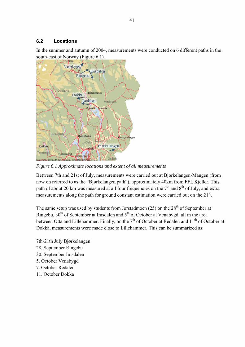
In the summer and autumn of 2004, measurements were conducted on 6 different paths in the south-east of Norway (Figure 6.1).

Figure 6.1 Approximate locations and extent of all measurements

Between 7th and 21st of July, measurements were carried out at Bjørkelangen-Mangen (from now on referred to as the “Bjørkelangen path”), approximately 40km from FFI, Kjeller. This path of about 20 km was measured at all four frequencies on the 7th and 8th of July, and extra measurements along the path for ground constant estimation were carried out on the 21st. The same setup was used by students from Jørstadmoen (25) on the 28th of September at Ringebu, 30th of September at Imsdalen and 5th of October at Venabygd, all in the area between Otta and Lillehammer. Finally, on the 7th of October at Redalen and 11th of October at Dokka, measurements were made close to Lillehammer. This can be summarized as: 7th-21th July Bjørkelangen 28. September Ringebu 30. September Imsdalen 5. October Venabygd 7. October Redalen 11. October Dokka

42

6.3 Noise

We wanted to estimate the noise in our measurements. This would give more confidentiality in the recorded data. It was also deemed necessary to investigate the spectrum just prior to measurement to avoid any interfering transmissions. We generally categorize noise into internal noise of the measurement setup (system dependent) and external noise that is either man-made or natural (not system dependent). We will concentrate on noise that can be analysed as white or near white spectrum regardless of physical origin, and disregarding interference. Curves of natural and man-made external noise are available in (26), and noise performance of the measurement equipment is typically available from the manufacturer. These could be used as a reference, but having actual measurements at the exact time and location gives better confidence in the results. Different types of measurements were done at each measurement site to estimate noise. Common to all is that only a single point in space and short period of time was measured, meaning that our estimate is accurate only within those limits, and may differ somewhat outside. The student measurements (site 1 to 5 in the tables) used the following analyzer setting:

• frequency span: 100 kHz, • Radio bandwidth 1000 Hz, • sweeptime 0.601s.

The Rx vehicle was close to the transmitter, and in some measurements, the Tx was switched on while logging, meaning that the spectrum of no signal/signal can be compared. In other measurements, the Tx was transmitting throughout the log. Below is an example log, Figure 6.2, where time is along the x-axis and a number of sweeps are carried out around the center frequency +/-(frequency span)/2. At sweep number 16, Tx starts transmitting, and a strong peak from its carrier frequency can be observed in the middle of each sweep.

43

Figure 6.2 Example Noise measurement log Figure 6.3 Example signal/noise spectrum

By averaging every sweep with and without this Tx carrier, we can get a picture of the statistics over a longer term as shown in Figure 6.3. We can see the obvious carrier at the center frequency, but we can also investigate any differences at its edges stemming from phase-noise or non-linear behaviour in the transmitter and receiver. Note that the number of blocks containing a transmitter tone (the 2nd half of Figure 6.2) as well as those that contain no such tone (pure noise, the first half of the same figure) is different at each site from 0 to a larger number, meaning that the accuracy is variable. The plotted “average noise level” in Figure 6.3 is an average (of dB-values) of the signal-less spectrum, and is considered an indicator of noise level for a relatively flat spectrum free of any obvious interferences. Note that this is the observed power in a given bandwidth of either 100 or 1000 Hz, while all signal measurements were carried out at 100 Hz bandwidth. We now have an estimate for noise signal power within a given bandwidth. What we need is the corresponding noise field strength within 100 Hz to match other measurements. Using formulas derived earlier, and assuming a white noise floor, we find: General formula for noise power within a bandwidth:

0

0noise

N kTP N B

==

Using “m” for measured values and “d” for desired values we express the desired noise power Pn,d within a desired bandwidth Bd using measured noise power Pn,m within bandwidth Bm:

44

, 0

0 ,

, 0

,

, 10 10

/

( / )10 log ( ) 10log ( )

n m m

n m m

n d d

n m d m

n m d m

P N BN P BP N B

P B BP B B

=

=

=

=

= + −

As we are interested in a bandwidth of 100 Hz we can further simplify:

, , 1010 log ( ) 20n d n m mP P B= − + From earlier calculations, we have that the E-field at the receiver can be found using measured antenna factor AF:

,[ / ] [ ] 107n dE dB V m P dBm AFμ = + +

Site F[MHz] 1 2 3 4 5 6 mean

3.172 18.8 16.6 17.7

9.2785 8.7 3.9 4.3 5.6

16.041 8.7 10.8 10.9 10.1

24.7815 29.8 25.8 27.7 30.6 24.5

Table 6.1 Estimated Field strength [dBμV/m]of noise including compensation for Rx Antenna Factor as a function of frequency [MHz] and Location in 100Hz bandwidths. Suitable for comparing with measurement data plots.

The rise in noise level in Figure 6.4 with frequency is not what one would expect from curves of natural noise. It is the result of compensating for non-uniform sensitivity as well as generally poor active antenna performance at 25 MHz.

45

Figure 6.4 Estimates of equivalent noise field strength within 100Hz bandwidth.

46

6.4 Spatial Fading

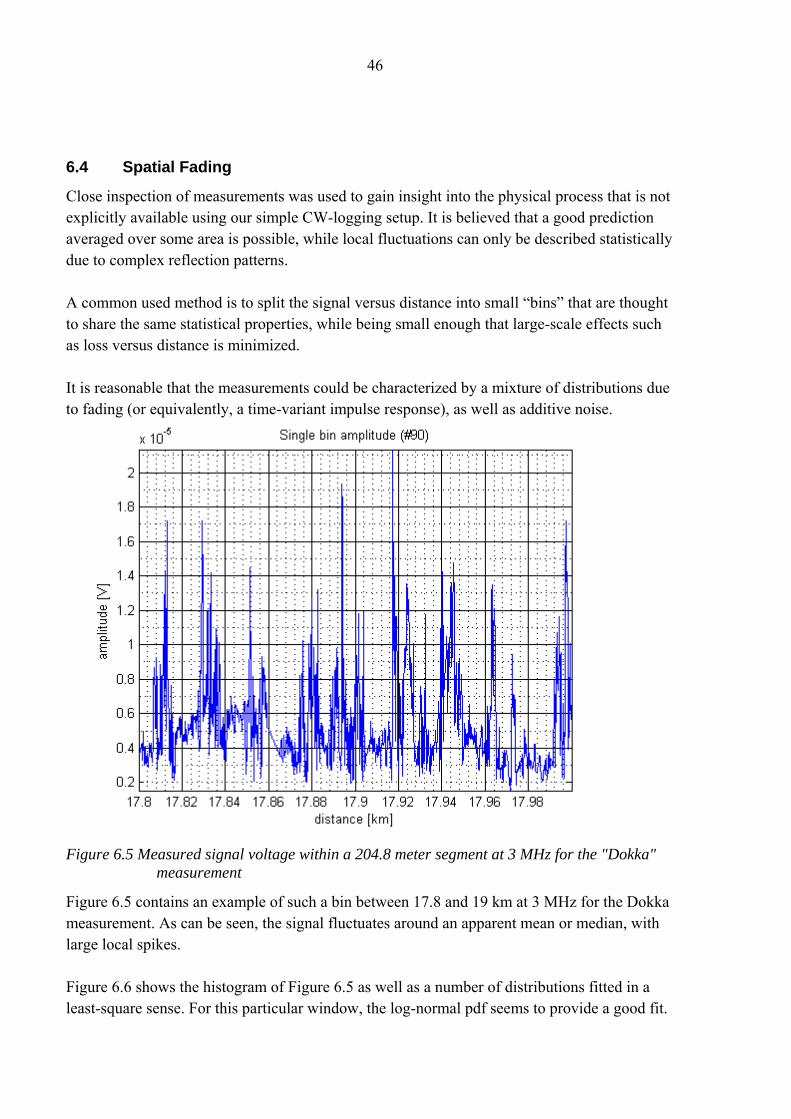
Close inspection of measurements was used to gain insight into the physical process that is not explicitly available using our simple CW-logging setup. It is believed that a good prediction averaged over some area is possible, while local fluctuations can only be described statistically due to complex reflection patterns. A common used method is to split the signal versus distance into small “bins” that are thought to share the same statistical properties, while being small enough that large-scale effects such as loss versus distance is minimized. It is reasonable that the measurements could be characterized by a mixture of distributions due to fading (or equivalently, a time-variant impulse response), as well as additive noise.

Figure 6.5 Measured signal voltage within a 204.8 meter segment at 3 MHz for the "Dokka"

measurement

Figure 6.5 contains an example of such a bin between 17.8 and 19 km at 3 MHz for the Dokka measurement. As can be seen, the signal fluctuates around an apparent mean or median, with large local spikes. Figure 6.6 shows the histogram of Figure 6.5 as well as a number of distributions fitted in a least-square sense. For this particular window, the log-normal pdf seems to provide a good fit.

47

Figure 6.6 Fitting common distributions to a 204.8 meter segment at 3 MHz for the "Dokka"

measurement

Figure 6.7 Fitting a polynome to measurements

48

For investigating statistics and frequency analysis of measurements, some kind of high-pass filtering could be beneficial. This is to remove large-area variation due to predictable distance-dependant losses, and possibly large-area fading to have a more rapidly varying residue consisting of fading and noise. A second-order polynome is fitted to measurements versus distance, using least squares to minimize the total error, see Figure 6.7 . The remaining signal can be observed in Figure 6.8 to be more “noise-like”, more or less flat, and with rapid variations. We can also observe that the signal is fluctuating more rapidly and with more high-frequency content for the last part, where the SNR is lower.

Figure 6.8 Residue after subtracting(in dB) polynome from measurements

In Figure 6.9, we have selected one of the residues in Figure 6.8 (both produce virtually identical results) for frequency analysis. The larger window contains windowed FFTs of the original signal taken at 204.8m bins (containing 2048 samples). Amplitude is colour-coded, where red corresponds to large amplitude and blue corresponds to a small amplitude. We are mainly interested in relative amplitude, so absolute references are not included. The y-axis contains logarithmic frequency from 0 (y=0) to fs/2 (top), where fs is the sampling rate. As the measurement is a function of distance, we are considering spatial frequency, or the number of cycles per meter. We can see that this is generally a low-pass function. In other words, there is more energy in slowly varying fluctuations than rapidly varying ones. This can also be seen from the window on the left, where each frequency has been summed across distance, to produce an averaged energy per frequency of the entire distance. The window on top shows the DC (zero-frequency) value of each bin, and we can see that it has been almost flattened.

49

Figure 6.9 Spectrogram for selected residue at 3 MHz. All values in dB (unknown ref).

We observe that the last part contains a wider “spectrum”, most probably due to lower SNR. We also observe a “cut-off” at a frequency of approximately 0.03 cycles/meter. This corresponds well to the Rayleigh multipath maximum frequency of 2/wavelength or 0.02 cycles/meter, indicated by a red line. This suggests that some fading mechanism is causing this variation. The actual probability density function is unknown, however.

Figure 6.10 Spectrogram for selected residue at 24.78 MHz

The measurement at 24.78 MHz was corrupted by noise from 6-8km onwards. By observing Figure 6.10 we can see that the same “maximum frequency” as was seen in the previous figure is evident in the first few km at a higher spatial frequency, corresponding to the higher carrier frequency.

50

Both plots have a drop of energy in the highest frequencies, above approximately 1 cycle/meter. This could be due to actual measurement samples being oversampled in the processing. Data are represented as sampled at 10 samples/meter, while actual data samplingrate vary down to a lower limit given by maximum receiver speed, some 3 samples/meter. The data have been linearly interpolated to produce the extra samples. This process should not introduce much high frequency content compared to white equipment noise. These plots are representative of their respective frequencies at other measurements. As a conclusion, it would seem that it is safe to filter raw measurement data at 2/wavelength to reduce noise without losing any measurement precision. Measurements at lower frequencies are more “oversampled” than higher frequencies, meaning that more samples can be averaged to reduce noise. The cause of fading can be any reflecting object close enough to the receiver, such as cars, power lines/lamp posts, buildings etc. No attempt is made at properly describing the PDF of measurements.

51

6.5 Measurements at each path

6.5.1 The Bjørkelangen path

Figure 6.11 Transmitter location

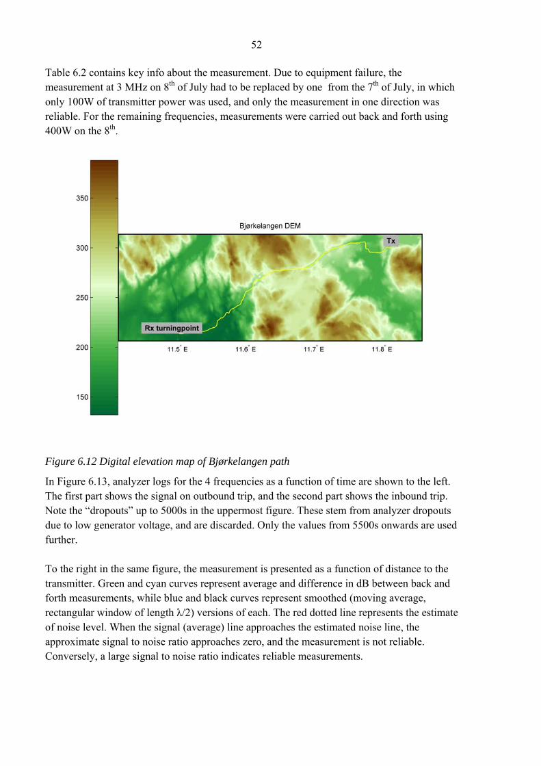
Measurements at Bjørkelangen on the 7th, 8th and 21st of July served as a test of equipment and procedures. As a result, more effort and time were spent on this dataset, and we will use these measurements as an introduction. All measurements can be found in appendix H. Figure 6.12 shows a bird’s-eye view of the terrain elevation on the site. The vertical bar to the left shows color-coding in meters. This is a relatively flat area with elevation ranging from 150 to 375 meters. The yellow line is constructed from the receiver vehicle GPS lat/lon logs, and represents the path that the receiver vehicle drove along. Grey text boxes “Tx” and “Rx turningpoint” represent the Tx location and the farthest point along the receiver path. As a rule, the receiver would start close to the transmitter, drive to “Rx turningpoint”, then return.

Table 6.2 Setupdata for Bjørkelangen measurement

Maximum distance 21.98km

Signal amplifier yes Tx position 59.9907N 11.8225E

Rx turningpoint 59.9265N 11.4490E frequency Start time

(day/month/hh:mm) Power amplifier setting

3.172 MHz 7/7/10:54 100W 9.2875 MHz 8/7/12:27 400W 16.041 MHz 8/7/13:42 400W 24.7815 MHz 8/7/15:05 400W

52

Table 6.2 contains key info about the measurement. Due to equipment failure, the measurement at 3 MHz on 8th of July had to be replaced by one from the 7th of July, in which only 100W of transmitter power was used, and only the measurement in one direction was reliable. For the remaining frequencies, measurements were carried out back and forth using 400W on the 8th.

Figure 6.12 Digital elevation map of Bjørkelangen path

In Figure 6.13, analyzer logs for the 4 frequencies as a function of time are shown to the left. The first part shows the signal on outbound trip, and the second part shows the inbound trip. Note the “dropouts” up to 5000s in the uppermost figure. These stem from analyzer dropouts due to low generator voltage, and are discarded. Only the values from 5500s onwards are used further. To the right in the same figure, the measurement is presented as a function of distance to the transmitter. Green and cyan curves represent average and difference in dB between back and forth measurements, while blue and black curves represent smoothed (moving average, rectangular window of length λ/2) versions of each. The red dotted line represents the estimate of noise level. When the signal (average) line approaches the estimated noise line, the approximate signal to noise ratio approaches zero, and the measurement is not reliable. Conversely, a large signal to noise ratio indicates reliable measurements.

53

The plots of difference can be seen as another test for reliability. A large difference indicates some sort of time variation on a time scale of minutes to an hour (the time difference between two runs). This could be due to noise, moving reflectors (cars, airplanes) or receiver antenna diagrams. High-frequency differences can be produced by errors in GPS position for the two runs compared, especially during deep fades when the signal derivative is large. By smoothing the error we get a visual impression of its low frequency components. Somewhat surprisingly, we see that the quality of measurements seems to increase markedly with lower frequency. Although 3 MHz was thought to propagate better than 24 MHz (less distance-dependant loss), both antenna length and natural noise floor curves was believed to counter this effect somewhat. The difference between instantaneous field strength and estimated noise floor (SNR) is at all times large for 3 MHz, decreasing with frequency until approaching zero (no discernible signal) from 10km onwards for the 25 MHz measurement. The difference between runs also increased with frequency (not visible at 3 MHz for this measurement, but the trend existed for all other measurements). This is perhaps more intuitive as fading phenomena should be more prominent at the higher frequency, and given a constant sampling-rate, the 3 MHz signal could be thought of as more highly over-sampled than those at higher frequencies.

54

Figure 6.13 Measured field strength vs time (left), field strength vs distance (right)

55

Figure 6.14 Measured field strengths for Bjørkelangen frequencies 3-25 MHz

Figure 6.14 shows the “smoothed average” curves for all frequencies simultaneously. The noise floor is indicated by a lighter color, seen below ~35dB for the purple line. In other words, the logged value is plotted, but indicated to be unreliable by the lighter color. For 25 MHz, all values from 10 km onwards are more or less flat, suggesting that we are measuring the noise floor and not a distance-dependent signal. Continuing the analysis, we want to make some kind of assumption that presents the data in a more manageable form. Here, we have chosen to use the GRWAVE prediction for “medium dry ground” from (8), and using the difference in dB, or residue for further analysis defined by:

,[ / ]err meas gr med dryE dB V m E Eμ −= −

Figure 6.15 shows the error using GRWAVE for the four frequencies (shifted downwards for visibility) in colors. In addition, Clearance-angle loss as well as Bullington diffraction losses are plotted in black for each frequency. As CLA is basically frequency independent (5), only the curve for 3 MHz is plotted. Bullington frequency-dependent diffraction loss is plotted in black and shifted equally to corresponding error plots.

56

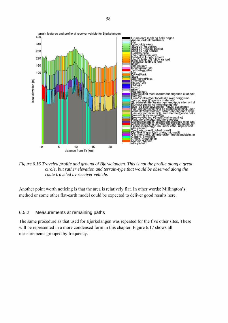
These curves are interesting as there seems to be a clear correlation between the shape of error residue and diffraction, even at 3 MHz. This would indicate that some diffraction model could indeed be used to improve smooth-earth prediction through-out the HF band. On the other hand, each measured curve has a “constant” shift that is individual for each frequency and each location. This is to be expected as the electrical characteristics vary both in frequency and space. It could be argued that the observed variation is due to local (on the receiver-side) variations in ground characteristics that coincidentally correlate well with calculated diffraction losses, or that there is some general physical correlation between “good/bad electrical land” and “low/high diffraction loss”, for instance steep, dry terrain compared to flat, wet terrain. The first case would seem unlikely, and easily negated by measuring several sites. The second case may be possible, but for practical purposes the actual physical reason may be less important than the actual improvement in prediction. The curves show a section from 16 km onwards of higher signal strength that increase with lower frequency that can only be partially explained by moving out of the obstruction shadow. It is believed that this is related to moving out of a forested area and into agricultural land. See Figure 6.16 for a representation of local elevation as well as ground type from three digital map sources stacked on top of each other in the figure.

57

Figure 6.15 Bjørkelangen residual error after subtracting GRWAVE prediction from

measurement using "medium dry ground"

Note that this is for the path traveled by the receiver, and not a great circle from point to point. This means that it is less relevant for analysing diffraction losses. Rather, it can be used to reveal zones of good or bad ground constants. The legend uses actual description from map files in Norwegian, and some descriptions are cut due to their length. For the Bjørkelangen path it would seem likely that signal levels would improve from 16 km onwards, given the luxury of hindsight and this map data. This is because agricultural land is known to have very beneficial conditions for groundwave propagation.

58

Figure 6.16 Traveled profile and ground of Bjørkelangen. This is not the profile along a great

circle, but rather elevation and terrain-type that would be observed along the route traveled by receiver vehicle.

Another point worth noticing is that the area is relatively flat. In other words: Millington’s method or some other flat-earth model could be expected to deliver good results here.

6.5.2 Measurements at remaining paths

The same procedure as that used for Bjørkelangen was repeated for the five other sites. These will be represented in a more condensed form in this chapter. Figure 6.17 shows all measurements grouped by frequency.

59

Figure 6.17 All measurements grouped into frequency, logarithmic distance axis. Color-coding is identical for each frequency. The first 6 plots are regular measurements, plots #7-8 are special short measurements for estimating ground parameters at Bjørkelangen, “Cymomotive force measure” stems from Tx power calibration and “sea”, “wet”, “dry” and “ice” are GRWAVE calculations for the ITU-T ground-types indicated. “ice” curves overlap “dry” curves for the given parameters.

We observe that the “cymomotive force measurement” approach the “sea” plot in the limit of zero distance for all frequencies. This is to be expected as we have calibrated the transmitter power to approach a 1kW monopole transmitter situated on a loss-less ground. As the distance increases, all measurements fall off (at different rates) from the near-ideal case that appears over sea. Field strengths seem to generally fall between “wet land” and “dry land”, validating both measurement methodology as well as calibration procedures. It seems that measurements at 3 and 25 MHz are better confined within those limits than those at 9 and 16 MHz for unknown reasons. It would make sense if signal levels were steadily falling with frequency as terrain roughness could no longer be ignored (GRWAVE does not take terrain roughness into consideration).

60

The plots are too dense to single out any measurements, but we can make some general considerations. The “thickness” indicates the variation from site to site. As long as the vertical spread is several tens of dB, we can safely assume that the potential of more precise prediction is considerable. As measurements are carried out at similar locations (inland south-east of Norway), a frequency planner may use the same ground parameters for all paths manually entered into for instance GRWAVE since conductivity/permittivity maps of Norway are rather coarse. The horizontal spread then indicates that for a given SNR, the real range could vary with a factor of 10, while a good prediction hopefully would lie somewhere between those extremes. We can also observe that one single measurement may “jump” from very good conditions to very bad conditions as a function of distance. In other words, there seems to be no single parameter as in GRWAVE, characterizing each location that can be used for improving predictions.

Figure 6.18 Relationship between CLA and prediction error

Figure 6.18 shows the residue, Eerr versus Clearance angle loss for one single location, Dokka. Lower frequencies are partially obscured by higher ones. Ideally, we should have that Eerr equals CLA. Although a lot of “noise” is present, there seems to be a trend going from lower

61

left to upper right. In other words, for locations where the smooth earth prediction is overly optimistic, giving a large negative error, there tends to be a large predicted diffraction loss. This can be more clearly seen to the right in the same figure, in which 1st, 2nd and 3rd order polynomes have been fitted, minimizing the squared error. Here, we can clearly see the trend mentioned.

Figure 6.19 Polynome fits to all 6 measurements

Figure 6.19 shows the mean of fitted polynomes for all 6 measurements. Here we can clearly see that the frequency independance of CLA is a simplified model. As the frequency increase, the (idealized) linear function connecting prediction error to diffraction losses gets steeper, indicating that obstruction losses increase with frequency. Figure 6.20 shows the rms-error defined as:

62

2,

1

1 ( ( ) ) , whereN

rms err err mean err meas predi

E E i E E E EN =

= − = −∑

for measured and predicted values Emeas and Epred. In this plot, error is calculated for each sample along the measured path, and a rms-value is obtained by squaring each value and taking the root of mean of those values.

Figure 6.20 RMS error using GRWAVE and using GRWAVE combined with Bullington

diffraction

Blue and green represent error using only GRWAVE smooth earth and medium dry ground. The sum of rms-error across frequencies range from ~30dB (Bjørkelangen) to ~65dB (Redalen-Lia), while the sum of mean rms error for all frequencies is somewhat more than 50 dB using this method. Red and yellow represent the rms error when a combination of GRWAVE and Bullington diffraction loss is used. As can be seen, summed mean rms error for all sites is in the range of 25 dB, or 25 dB less than using GRWAVE only. The conclusion so far is that there is a significant correlation between the prediction error using accepted smooth earth models and even very simple diffraction models. We have also shown that this correlation can be exploited to reduce the expected error. We will now delve deeper into models presented in earlier chapters to further analyse measurements.

63

6.5.3 Characterising measurements using a wider range of models

Chapter 6.5.2 contained a characterization of measurements and basic models in a statistical sense, indicating that there is reason to include terrain elevation and diffraction effects when predicting HF groundwave propagation, even at the lower region of the HF spectrum. This chapter will use a wider array of models and discuss specific phenomena encountered at different locations.

Figure 6.21 Measurement and predictions for Bjørkelangen, 3 MHz

Figure 6.21 and Figure 6.22 display the measurements presented in chapter 6.5.1 along with predictions from chapter 3 for 3 MHz and 16 MHz, respectively. Additionally, a naive model assuming only diffraction losses and loss-free ground (Lfree – bullington diffraction) is shown to be unrealistically optimistic. No assumptions are made to the influence of changes in ground constants; medium dry ground is used for the entire path. Comparing the two plots, we see that:

• At 3 MHz, the improved field strength beyond 15 km can not be explained by terrain-type effects

• At 16 MHz, the variations in the measurement seems to be sufficiently modeled by terrain dependence alone, although effective terrain constants are probably somewhat optimistic.

64

The “B&L” model suppress dependency on diffraction to the point where we are approaching a smooth earth model in those two examples. At 16 MHz, wagslab and “clearance angle” or “Millington - bullington” seems to make a better fit.

Figure 6.22 Measurement and predictions for Bjørkelangen, 16 MHz

These two examples are consistent with the idea that smooth earth ground-losses are most important at low frequencies, while the relative importance of diffraction losses increase with frequency. Figure 6.23 shows a clear correlation between diffraction-related losses and variation in received field strength. The ground parameters used (medium dry ground) may be somewhat optimistic. Using very dry ground, for instance, would shift all prediction curves down somewhat. However, it seems that the “B&L”-model suppress variation due to the section of better conditions between 7 and 15 km.

65

Figure 6.23 Measurement and predictions for Imsdalen, 3 MHz

66

7 CONCLUSION AND RECOMMODATIONS

This research has indicated that improved prediction is possible for HF groundwave propagation by including diffraction-type effects as well as changes in ground constants, even in the lower part of the HF band. The WAGSLAB model gives very good prediction when it is stable. However, problems occur for large distances combined with high frequencies. This problem is difficult to reveal other than using manual analysis of curves. A simple, stable model was suggested that can improve predictions compared to a smooth-earth model for the limited case of ground-based terminals, this improved model would be at neglible computation cost. A serious limitation to any prediction will be the availability of maps of ground conductivity/relative permeability. Using available agriculture vector maps was investigated, although this is an area of further research. For practical field use, it is impractical to measure directly those constants. Further research and improvement of existing conductivity/permittivity maps would provide benefit for theoretical as well as practical applications. It is believed that more insight could be gained by using more specialized measurement equipment. Direct measurement of path impulse response through some larger bandwidth transmitter/receiver could reveal the physical mechanism behind fading and its sources. A true mobile (back pack) receiver could be used for obtaining 2d area-coverage.

67

References (1) A. N. Sommerfeld (1909): Propagation of Waves in Wireless Telegraphy, Ann. Phys.

(Leipzig) 28, 665-737. (2) K. A. Norton (1936): "The Propagation of Radio Waves over the Surface of the Earth

and in the Upper Atmosphere", Proceedings of the IRE 24, 1367-1387. (3) G. Millington (1949): "Groundwave Propagation Over an Inhomogeneous Smooth

Earth", Proceedings of the IEE Pt. III, 53-64. (4) J. R. Wait (1998): The Ancient and Modern History of EM Ground-Wave Propagation,

IEEE Antennas and Propagation Magazine 40, 5, 7-24. (5) B. Hvesser, O. Grønnerud, J. Sander (2004): TERRENGETS PÅVIRKNING AV

JORDBØLGEN PÅ HF - måleresultater og analyse, FFI/RAPPORT-2004/01135, UNCLASSIFIED.

(6) J. Zenneck (1907): "Propagation of Plane EM Waves Along a Plane Conducting

Surface", Ann. Physics 23, 846-866. (7) Å. Blomquist (1968): RADIOVÅGORS UTBREDNING - JORDYTANS

INNVERKAN, Försvarets forskningsanstalt (FOA), Stockholm, 6-17. (8) Recommendation ITU-R P.527-3 "Electrical characteristics of the surface of the earth"

(1978-1982-1990-1992). (9) Recommendation ITU-R P.879-1 "Methods for estimating effective electrical

characteristics of the surface of the Earth" (1986). (10) S. Rotheram (1981): Ground Wave Propagation, Proceedings of the IEE 128, Pt. F, 275-

295. (11) Recommendation ITU-R P.368-7 "Ground-wave propagation curves for frequencies

between 10 kHz and 30 MHz" (1992). (12) R. J. King (1976): Wave-Tilt Measurements, IEEE Transactions on Antennas and

Propagation, 115-119. (13) G. Millington, G. A. Isted (1950): "Ground-wave propagation over an inhomogeneous

Earth. Part 2 Experimental evidence and practical implications", IEE Proceedings 97, 209-222.

(14) K.N. Stokke (1975): Some graphical considerations on Millington’s method for

calculating field strength over inhomogeneous earth, telecommunication journal 42, III. (15) B. Asp, G. Eriksson, P. Holm (1997): Detvag-90 - Final Report, FOA Defence Research

Establishment, Linkøping, 28.

68

(16) M. P. M. Hall, L. W. Barclay, M. T. Hewitt (1996): Propagation of Radiowaves, The Institution of Electrical Engineers, London, 307-321.

(17) Knut N. Stokke (1977): Resultater fra LF/MF-konferansen, Telektronikk, 4, 309. (18) ITU (2005): [http://www.itu.int/ITU-R/software/study-

groups/rsg3/databanks/troposph/index.html]. (19) K. I. Hvidsten, B. H. Farsund (2004): The influence of mountainous and irregular terrain

on HF ground wave propagation, proc., Nordic Shortwave Conference, Fårø, 10-12.aug. (20) Å. Blomquist, L. Ladell (1973): Prediction and Calculation of Transmission Loss in

Different Types of Terrain, FOA, Stockholm. (21) D.A. Hill (1982): HF ground wave propagation over forested and built-up terrain, NTIA

Technical Reports 82-114, Boulder. (22) K.N. Stokke (1984): Ground conductivity measurements, telecommunication journal 51,

XI. (23) (2005): http://www.plan.aau.dk/~pce/. (24) (2005): European space agency, www.esa.int. (25) A. Johnsen M. H. Aaser (2004): Modellering av Radiobølgeutbredelse for HF,

Hovedprosjektoppgave Hærens Ingeniørhøyskole/Jørstadmoen. (26) Recommendation ITU-R P.372-7 (2001). (27) Norwegian Meteorological Institute (2005): www.met.no. (28) R.H. Ott (1971): A new method for predicting HF ground wave attenuation over

inhomogeneous irregular terrain, OT/ITS RR 7 , Boulder. (29) K. N. Stokke (1984): Ground conductivity measurements, telecommunication journal 51,

Xi, 611-613.

69

Bibliography not referred to in the text J. C. Schelleng, C. R. Burrows and E. B. Ferrell (1933): Ultra-short-wave Propagation, proceedings of the IRE 21, 3. P. Holm (1993): DETVAG-90 Användning av markvågsprogrammet GRWAVE i vågutbredningsmodellen DETVAG, FOA rapport, Linköping K. Bullington (1977): Radio Propagation at Frequencies Above 30 Megacycles, proceedings of the IRE – Waves and Electrons Section 1947 pp. 1122-1136. L. Sevgi, F. Akleman, L. B. Felsen (2002): Groundwave Propagation Modelling: Problem-Matched Analytical Formulations and Direct Numerical Techniques, IEEE Antennas and Propagation Magazine 44, 1, 55-75.

70

APPENDIX

A ABBREVIATIONS AND ACRONYMS

AF – Antenna Factor AM – Amplitude Modulation CEP - Circular Error Probability CLA – Clearance Angle dB – decibel dBm – dB over one milliwatt dBμV – dB over one micro volt dGPS – Differential GPS EGNOS - European Geostationary Navigation Overlay EIRP - Effective Isotropic Radiated Power EM – Electro-magnetic EMRP - Effective Monopole Radiated Power ERP - Effective Radiated Power GPS – Global Positioning System HF – High Frequency ITU – the International Telecommunications Union Lat - Lattitude LF – Low Frequency Lon - Longitude MF – Medium Frequency mm - millimeter NMEA - National Marine Electronics Association PC – Personal Computer PDF – Probability density function Rms – Root-Mean-Square Rx – (radio) Receiver S/A - Selective Availability SNR – Signal to Noise Ratio Tx – (radio) Transmitter VHF – Very High Frequency WAAS - Wide Area Augmentation System/ System

71

B MAPS AND METEOROLOGICAL DATA

Sources of map data and a short description of map format

B.1 Digital elevation maps

Forsvarets militærgeografiske tjeneste (Norwegian Military Geographic Service) Dted2 Norge Approximately 30 meter resolution

B.2 N50 vector maps

Forsvarets militærgeografiske tjeneste (Norwegian Military Geographic Service) UTM32, WGS84 shape-files

B.3 Agriculture/forest productivity maps

NIJOS, Norsk institutt for jord- og skogkartlegging (Norwegian Institute of Land Inventory) www.nijos.no

B.4 Soil geology maps

NGU, Norges Geologiske Undersøkelse www.ngu.no shape-format, wgs84 Oslo/Akershus (N50) Hedmark (N250) Oppland (N250)

B.5 Solid rock geology maps

NGU, Norges Geologiske Undersøkelse

72

C METEOROLOGY

Recorded meteorological data are available from (27). Temperatures and precipitation for the relevant months in 2004 are presented here for the closest stations, Blindern in Oslo and Haugedalen in Rena. No attempt at modelling the complex relationship between precipitation, ground/geology, temperature and ground moisture content is carried out. However, as it has been indicated that the last 7 days of rain seem to be most important for our purpose, inspecting the graphs may give some background into evaluating the measurements. Figure C.1 and C.2 show meteorological data for the two meteorological stations, with measurement dates marked with blue arrows/text. The Bjørkelangen measurement was carried out at temperatures of approximately 10 degrees above the other measurements. While measuring in Dokka, the daily average was close to zero, but during the day (when measurements were taken), it was up to 7.5 degrees. (Copyright The Norwegian meteorological institute, www.met.no)

Figure C.1 Daily average temperature (Copyright The Norwegian meteorological institute,

www.met.no)

73

It is seen in Figure C.2 that the last measurements of Bjørkelangen as well as Venabygd and Redalen were carried out at or within two days of rainfall of 15.3 and 25.9 mm/day respectively. Less precipitation is observed preceding the other measurements.

Figure C.2 Daily precipitation (Copyright The Norwegian meteorological institute, www.met.no)

74

D CALIBRATION DOCUMENTATION FROM NEMKO COMLAB

NEMKO COMLAB AS Prosjekt 04/722/FFI Målingene ble foretatt ved Gjølsen gård på Romerike. Målestrekning var 100 m uten hindringer i avstand 500 m fra målestrekningen. Bakken er åkerland med fuktig leirjord. Senderen var montert på egen bil med piskantenne på 5 m påmontert biltaket. Mottakerantenna var aktiv pisk på ca 60 cm montert på biltaket på mottakerbilen. Dessuten var det montert egen mottakerforsterker. Målingene ble foretatt på kabel ut fra mottakerforsterkeren. Måleresultater med 100 W setting på forsterker på sendesiden. Frekvens, MHz

Mottakernivå, VRx dBμV

Feltstyrke, E dBμV/m

Beregnet utstrålt effekt, Watt EIRP

Mottaker antennefaktor, AF dB

Mottaker antennegain dBi

3,17203 84,1 106,7 15,6 22,6 -42,3 9,2875 95,5 114,9 103,0 19,4 -29,8 16,041 93,3 113,4 72,9 20,1 -25,7 24,781 80,2 108,7 24,7 28,5 -30,4 Antennefaktor er definert som: E (dBμV/m) = VRx (dBμV) + AF (dB) Utstrålt effekt P (EIRP) beregnes ut fra mottatt feltstyrke E: E = (30xP)1/2/m Hvor m er måledistansen i m, P ustrålt effket (isotropisk) i Watt og E feltstyrke i V/m. Mottakergain G (dBi, isotropisk gain) er definert som AF = -29,77 + 20log(MHz) – G (dBi) Instrumenter: Loop antenne R&S HFH 2-Z2 Målemottaker R&S ESH 2 Spektrumanalysator hp 8562B (FFI) Nemko Comlab AS 6.07.2004 Egil Hauger

75

E CONVERTING SIGNAL VOLTAGE TO SIGNAL POWER CALIBRATION

Using: VRx (dB) = 20*log10{ VRx, V

/ VRef, V} VRx (V) = 10-6 * 10^{ VRx,dBμV/20} Using Ohms law we have that: P (dBm) = 10*log10{[ VV

2/Z]/PRef,W} PRx (dBm) = 10*log10{[ VRx, V

2/Z]/10-3} Assume Z = 50 Ohm and solve for PRx (dBm) : PRx (dBm) = 10*log10{[[10-6 * 10^{ VRx,dBμV /20}]2/Z]/10-3} = 10*log10{10-9 * 10^{VRx,dBμV/10}/Z} = VRx,dBμV + 10*log10{10-9/Z} = VRx,dBμV - 107 So the field strength can be expressed by signal power, measured antenna factor and a constant: E = VRx,dBμV + AF = PRx dBm + 107 + AF [dBμV/m] Where kf = 107 + AF is the value that we have to add to logged signal power.

76

F LIST OF EQUIPMENT Mercedes Benz Geländewagen containing:

• HAiCOM HI-204E GPS receiver • DUK antennen AAD 2/2 Active antenna unit (Power and selector) • DUK antennen STA 5 A Active aerial with amplifier (monopole) • Hewlett Packard 8562B Analyzer • Industrial PC

Siemens HF-3 mobile station containing:

• Siemens CHX200 RX/TX radio • Siemens antenna tuner • Siemens CHX200 PA400 Power amplifier • 6 m vertical monopole

77

G SENSITIVITY TO CONDUCTIVITY AND PERMITTIVITY AT 0.3, 3 AND 30 MHZ

10 km 100 km

0.3 MHz

3

MHz

30 MHz

Figure G.1 GRWAVE prediction for conductivities and permittivities at 10 and 100 km, 0.3, 3 and 30 MHz. ITU-values are inserted as circles

78

H MEASUREMENTS AND PREDICTIONS

79

80

81

82

83

84

85

86

87

88

89