71
FFTs in Graphics and Vision Invariance of Shape Descriptors 1

FFTs in Graphics and Vision
Invariance of Shape Descriptors
1

Outline
• Math Overview Translation and Rotation Invariance
The 0th Order Frequency Component
• Shape Descriptors
• Invariance
2

Translation Invariance
Given a function 𝑓 in 2D, we obtain a translation
invariant representation of the function by storing
the magnitudes of the frequency components:
𝑓 𝑥, 𝑦 =
𝑙,𝑚=−∞
∞
𝑓 𝑙, 𝑚𝑒𝑖 𝑙𝑥+𝑚𝑦
2𝜋
⇓ 𝑓(𝑙, 𝑚) 𝑙, 𝑚 ∈ ℤ
3

Rotation Invariance (Circle)
Given a function 𝑓 𝜃 on a circle, we obtain a
rotation invariant representation by storing the
magnitudes of the frequency components:
𝑓 𝜃 =
𝑙=−∞
∞
𝑓 𝑙𝑒𝑖𝑙𝜃
2𝜋
⇓ 𝑓(𝑙) 𝑙 ∈ ℤ
4

Rotation Invariance (2D)
Given a function 𝑓(𝑥, 𝑦) in 2D, we obtain a
rotation invariant representation of 𝑓 by: Expressing 𝑓 in polar coordinates:
𝑓𝑟 𝜃 = 𝑓(𝑟 ⋅ cos 𝜃 , 𝑟 ⋅ sin 𝜃)
Radius
Angle
5
𝑓𝑟1𝜃 𝑓𝑟2
𝜃

Rotation Invariance (2D)
Given a function 𝑓(𝑥, 𝑦) in 2D, we obtain a
rotation invariant representation of 𝑓 by: Expressing 𝑓 in polar coordinates:
𝑓𝑟 𝜃 = 𝑓(𝑟 ⋅ cos 𝜃 , 𝑟 ⋅ sin 𝜃)
Expressing each radial restriction in terms of its
Fourier decomposition:
𝑓𝑟 𝜃 =
𝑙=−∞
∞
𝑓𝑟 𝑙𝑒𝑖𝑙𝜃
2𝜋
Storing the magnitude of the frequency
components of the different radial restrictions: 𝑓𝑟(𝑙) ⋅ 2𝜋𝑟 𝑙 ∈ ℤ, 𝑟 ∈ [0,1]
6
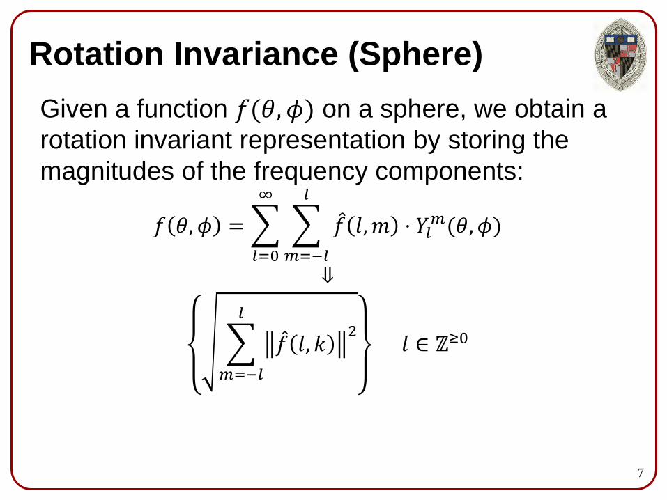
Rotation Invariance (Sphere)
Given a function 𝑓(𝜃, 𝜙) on a sphere, we obtain a
rotation invariant representation by storing the
magnitudes of the frequency components:
𝑓 𝜃, 𝜙 =
𝑙=0
∞
𝑚=−𝑙
𝑙
𝑓 𝑙, 𝑚 ⋅ 𝑌𝑙𝑚(𝜃, 𝜙)
⇓
𝑚=−𝑙
𝑙
𝑓 𝑙, 𝑘2
𝑙 ∈ ℤ≥0
7

Rotation Invariance (3D)
Given a function 𝑓(𝑥, 𝑦, 𝑧) in 3D, we obtain a
rotation invariant representation of 𝑓 by: Expressing 𝑓 in spherical coordinates:
𝑓𝑟 𝜃, 𝜙 = 𝑓(𝑟 ⋅ cos 𝜃 ⋅ sin 𝜙 , 𝑟 ⋅ cos 𝜙 , 𝑟 ⋅ sin 𝜃 ⋅ sin 𝜙)
8

Rotation Invariance (3D)
Given a function 𝑓(𝑥, 𝑦, 𝑧) in 3D, we obtain a
rotation invariant representation of 𝑓 by: Expressing 𝑓 in spherical coordinates:
𝑓𝑟 𝜃, 𝜙 = 𝑓(𝑟 ⋅ cos 𝜃 ⋅ sin 𝜙 , 𝑟 ⋅ cos 𝜙 , 𝑟 ⋅ sin 𝜃 ⋅ sin 𝜙)
Expressing each radial restriction in terms of its
spherical harmonic decomposition:
𝑓𝑟 𝜃, 𝜙 =
𝑙=0
∞
𝑚=−𝑙
𝑙
𝑓𝑟 𝑙, 𝑚 ⋅ 𝑌𝑙𝑚 𝜃, 𝜙
Storing the size of the frequency components
coefficients of the different radial restrictions:
𝑚=−𝑙
𝑙
𝑓𝑟 𝑙, 𝑚2
⋅ 4𝜋𝑟2 𝑙 ∈ ℤ≥0, 𝑟 ∈ [0,1]
9

The 0th Order Frequency Component
Given a function on the circle 𝑓 𝜃 , we can
express the function in terms of its Fourier
decomposition:
𝑓 𝜃 =
𝑙=−∞
∞
𝑓 𝑙𝑒𝑖𝑙𝜃
2𝜋
What is the meaning of the 0th order frequency
component?
10

The 0th Order Frequency Component
The 𝑙th frequency is the dot product of the function
with the 𝑙th complex exponential:
𝑓 𝑙 = 𝑓 𝜃 ,𝑒𝑖𝑙𝜃
2𝜋=
0
2𝜋
𝑓 𝜃 ⋅𝑒−𝑖𝑙𝜃
2𝜋𝑑𝜃
So the 0th frequency component is:
𝑓 0 =1
2𝜋
0
2𝜋
𝑓 𝜃 𝑑𝜃
11
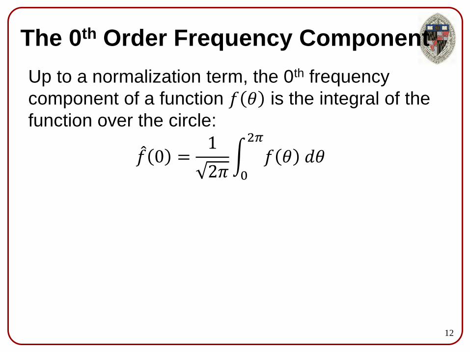
The 0th Order Frequency Component
Up to a normalization term, the 0th frequency
component of a function 𝑓 𝜃 is the integral of the
function over the circle:
𝑓 0 =1
2𝜋
0
2𝜋
𝑓 𝜃 𝑑𝜃
12

The 0th Order Frequency Component
Given a function on the sphere 𝑓 𝜃, 𝜙 , we can
express the function in terms of its spherical
harmonic decomposition:
𝑓 𝜃, 𝜙 =
𝑙=0
∞
𝑚=−𝑙
𝑙
𝑓 𝑙, 𝑚 ⋅ 𝑌𝑙𝑚(𝜃, 𝜙)
What is the meaning of the 0th order frequency
component?
13

The 0th Order Frequency Component
The (𝑙, 𝑚)th frequency component is computed by
taking the dot product of the function with the
(𝑙, 𝑚)th spherical harmonic: 𝑓 𝑙, 𝑚 = ⟨𝑓 𝜃, 𝜙 , 𝑌𝑙
𝑚(𝜃, 𝜙)
So the 0th frequency component is:
𝑓 0,0 =1
4𝜋
𝑝 =1
𝑓 𝑝 𝑑𝑝
14

The 0th Order Frequency Component
Up to a normalization term, the 0th frequency
component of a function 𝑓 𝜃, 𝜙 is the integral of
the function over the sphere:
𝑓 0,0 =1
4𝜋
𝑝 =1
𝑓 𝑝 𝑑𝑝
15

The 0th Order Frequency Component
Note:
In the case that the function 𝑓 is positive the 0th
frequency coefficient will also be positive: 𝑓(0) = 𝑓 0
𝑓(0,0) = 𝑓 0,0
16

Outline
• Math Overview
• Shape Descriptors Shape Histograms (Ankerst et al.)
Shape Distributions (Osada et al.)
Extended Gaussian Images (Horn)
• Invariance
17
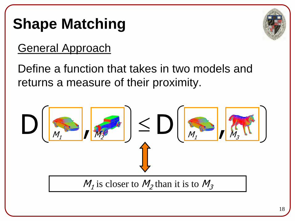
Shape Matching
General Approach
Define a function that takes in two models and
returns a measure of their proximity.
D , D ,M1 M1 M3M2
M1 is closer to M2 than it is to M3
18

Shape Descriptors
Challenge
It is difficult to match shapes directly: Different triangulations of the same shape
Different shapes have different genus
The same shape may be in different poses
Etc.
19

Shape Descriptors
Solution
Represent shapes by a structured abstraction that
represents every shape in the same domain.
Descriptors
3D ModelsD ,
D ,20

Outline
•Math Overview
• Shape Descriptors Shape Histograms (Ankerst et al.)
Shape Distributions (Osada et al.)
Extended Gaussian Images (Horn)
• Invariance
21

Shape Histograms
Approach
• Decompose space into concentric shells
• Store how much of the shape falls into each of
the shells
22

Shape Histograms
Properties
• Each shape is represented by 1D array of
values.
• The representation is invariant to rotation
23

Outline
• Math Overview
• Shape Descriptors Shape Histograms (Ankerst et al.)
Shape Distributions (Osada et al.)
Extended Gaussian Images (Horn)
• Invariance
24

D2 Shape Distributions
Approach
Avoid the whole problem of tesselation, genus,
etc. by building the shape descriptor from random
samples from the surface of the model:
Triangulated Model Point Set
25

D2 Shape Distributions
Key Idea
Use the fact that the distance between pairs of
points on the model does not change if the model
is translated and/or rotated.
𝑝2
𝑝1𝑇 𝑝1
𝑇(𝑝2)
26
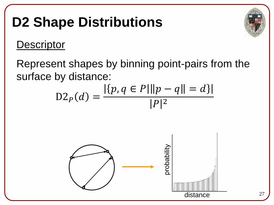
D2 Shape Distributions
Descriptor
Represent shapes by binning point-pairs from the
surface by distance:
D2𝑃 𝑑 =𝑝, 𝑞 ∈ 𝑃 𝑝 − 𝑞 = 𝑑
𝑃 2
distance 27

D2 Shape Distributions
Properties
• Each shape is represented by 1D array of
values.
• The representation is invariant to translations
and rotations
28

Outline
• Math Overview
• Shape Descriptors Shape Histograms (Ankerst et al.)
Shape Distributions (Osada et al.)
Extended Gaussian Images (Horn)
• Invariance
29

Extended Gaussian Images
Approach
Use the fact that every point on the surface has a
position and a normal.
Triangulated Model Oriented Point Set
30

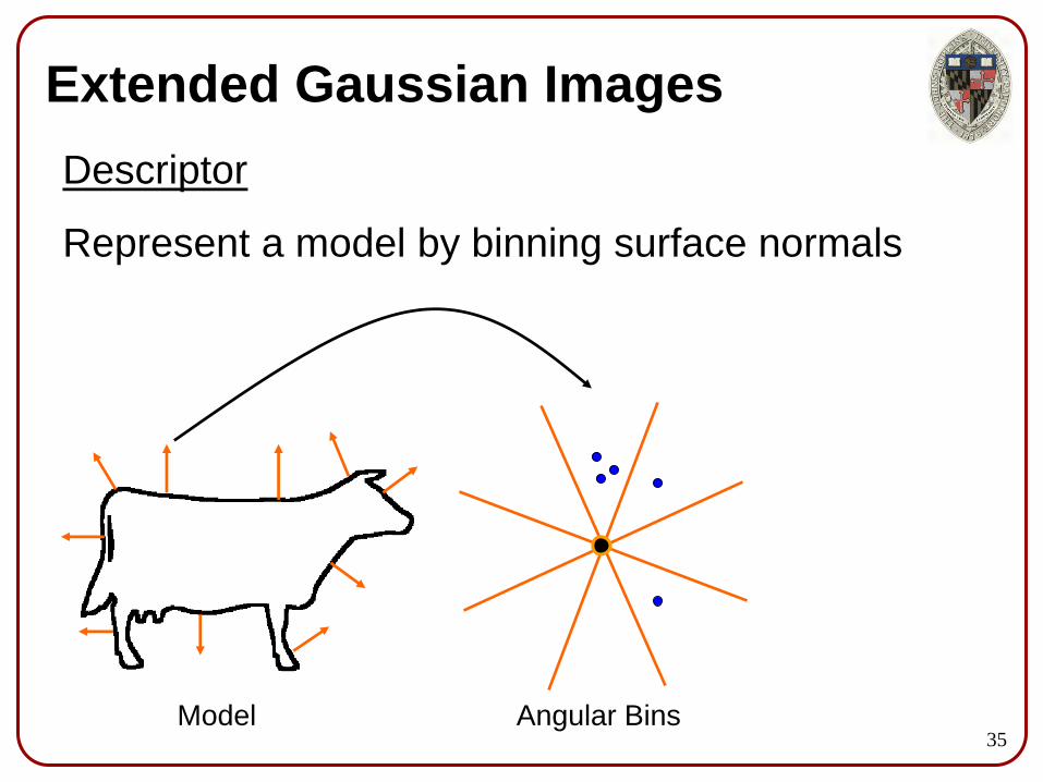
Extended Gaussian Images
Descriptor
Represent a model by binning surface normals
Model Angular Bins31

Extended Gaussian Images
Descriptor
Represent a model by binning surface normals
Model Angular Bins32

Extended Gaussian Images
Descriptor
Represent a model by binning surface normals
Model Angular Bins33

Extended Gaussian Images
Descriptor
Represent a model by binning surface normals
Model Angular Bins34
Extended Gaussian Images
Descriptor
Represent a model by binning surface normals
Model Angular Bins35

Extended Gaussian Images
Descriptor
Represent a model by binning surface normals
Model EGI36

Extended Gaussian Images
Properties
• A 2D curve / 3D surface is represented by a
histogram over a circle / sphere.
• The representation is invariant to translations.
37

Outline
• Math Overview
• Shape Descriptors
• Invariance
38

Normalization vs. Invariance
We say that a shape representation is normalized
with respect to translation / rotation if the shape is
placed into a canonical pose.
39

Normalization vs. Invariance
We say that a shape representation is normalized
with respect to translation / rotation if the shape is
placed into a canonical pose.
Example:
We can normalize for translation by moving the
surface so that the center of mass is at the origin.
40

Normalization vs. Invariance
We say that a shape representation is invariant
with respect to translation / rotation if the
representation discards information that depends
on translation / rotation.
41

Invariance
We have seen a general method for making
functions invariant to translation and rotation.
42

Invariance
Translation:
Compute the Fourier decomposition and store
just the magnitudes of the Fourier coefficients.
Cartesian Coordinates
𝑓 𝑥, 𝑦, 𝑧 =
𝑙,𝑚,𝑛
𝑓𝑙,𝑚,𝑛 ⋅𝑒𝑖 𝑙𝑥+𝑚𝑦+𝑧𝑛
2𝜋 1.5
𝑓𝑙,𝑚,𝑛 𝑙,𝑚,𝑛
Translation Invariant Representation𝑧𝑥
𝑦
43
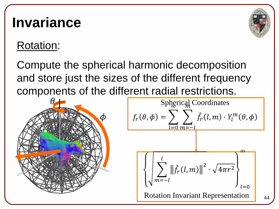
Invariance
Rotation:
Compute the spherical harmonic decomposition
and store just the sizes of the different frequency
components of the different radial restrictions.Spherical Coordinates
𝑓𝑟 𝜃, 𝜙 =
𝑙=0
∞
𝑚=−𝑙
𝑚
𝑓𝑟 𝑙, 𝑚 ⋅ 𝑌𝑙𝑚 𝜃, 𝜙
𝑚=−𝑙
𝑙
𝑓𝑟 𝑙, 𝑚2
⋅ 4𝜋𝑟2
𝑙=0
∞
Rotation Invariant Representation
r
𝜃
𝜙
44

Overblown Claim
All methods that represent 3D shapes in either a
translation-invariant or rotation-invariant method
implicitly use these invariance approaches.
45

Goal
Given the three shape descriptors: Shape Histograms
Shape Distributions
Extended Gaussian Images
• How does the descriptor obtain its invariance?
• How can the descriptiveness of the descriptor
be improved while maintaining invariance?
46

Shape Histograms
This shape descriptor represents a 3D shape by a
1D histogram.
It is obtained by binning points by their distance
from the center and is rotation invariant.
47

Shape Histograms
The shape histogram starts by representing the
surface by a 3D function, obtained by rasterizing
the boundary into a voxel grid: A voxel has value 1 if intersects the boundary
A voxel has value 0 otherwise.
ModelRasterization
48

Shape Histograms
The shape histogram can then be obtained by
setting the value of the bin corresponding to
radius 𝑟 equal to the “size” of the rasterization
restricted to the sphere of radius 𝑟:
ShapeHistogram 𝑟 = 𝑝 =𝑟
Raster 𝑝 𝑑𝑝
49

Shape Histograms
We can express the rasterization in spherical
coordinates:𝑅 𝑟, 𝜃, 𝜙 = Raster(𝑟 ⋅ cos 𝜃 ⋅ sin 𝜙 , 𝑟 ⋅ cos 𝜙 , 𝑟 ⋅ sin 𝜃 ⋅ sin 𝜙)
Then, for each radius, we get a spherical function:
𝑅𝑟 𝜃, 𝜙 = 𝑅(𝑟, 𝜃, 𝜙)
Which we can express as:
𝑅𝑟 𝜃, 𝜙 =
𝑙=0
∞
𝑚=−𝑙
𝑙
𝑅𝑟 𝑙, 𝑚 ⋅ 𝑌𝑙𝑚(𝜃, 𝜙)
50
Shape Histograms
In this formulation, the value of the shape
histogram at a radius of 𝑟 is the value of the 0th
spherical harmonic coefficient:*
ShapeHistogram 𝑟 = 𝑅𝑟 0,0 ⋅ 4𝜋𝑟2
*The scale factor of 4𝜋𝑟2 accounts for the fact
that the area of the sphere of radius 𝑟 is 4𝜋𝑟2.
51

Shape Histograms
So the shape histogram obtains its rotation
invariance by storing the (size of the) 0th order
frequency component:
ShapeHistogram 𝑟 = 𝑅𝑟 0,0 ⋅ 4𝜋𝑟2
Extension:
We can obtain a more descriptive representation,
without giving up rotation invariance, by storing
the size of every frequency component:
EShapeHistogram 𝑟, 𝑙 =
𝑚=−𝑙
𝑙
𝑅𝑟 𝑙, 𝑚2
⋅ 4𝜋𝑟2
52

D2 Shape Distribution
This shape descriptor represents a 3D shape by a
1D histogram.
It is obtained by binning point-pairs by their
distance, and is both translation and rotation
invariant.
D2 Distribution
3D Model
𝑝
𝑞
Distance
53

D2 Shape Distribution
Let’s consider the rotation invariance first.
54

D2 Shape Distribution
One way to think of the D2 shape descriptor is by
binning the difference vector between pairs of
points on the surface:
3D Model
𝑞
𝑝
Binned Difference Vectors 55

D2 Shape Distribution
One way to think of the D2 shape descriptor is by
binning the difference vector between pairs of
points on the surface.
Then the shape distribution can be obtained by
computing the Shape Histogram of the binning:
3D Model Binned Difference VectorsDistance 56

D2 Shape Distribution
As with the Shape Histogram, the D2 Shape
Distribution can be realized by storing 0th order
frequency components of the spherical harmonic
decomposition.
Extension:
As with the Shape Histogram the representation
can be made more descriptive, without sacrificing
rotation invariance, by storing the size of every
frequency component.
57
D2 Shape Distribution
This accounts for the rotation invariance of the D2
Shape Distribution.
What makes it translation invariant?
58

D2 Shape Distribution
The Shape Distribution is computed from the
binning of point-pair differences. How is this
function computed?
3D Model
𝑞
𝑝
Binned Difference Vectors 59

D2 Shape Distribution
A point 𝑞 on the surface will contribute to bin 𝑣 if
the point 𝑞 − 𝑣 is also on the surface.
3D Model
𝑞
𝑝
Binned Difference Vectors
𝑣 = 𝑞 − 𝑝
60

D2 Shape Distribution
Once again, we consider the rasterization of the
surface into a regular voxel grid.
ModelRasterization
61

D2 Shape Distribution
A point 𝑞 on the surface will contribute to bin 𝑣 if
the point 𝑞 − 𝑣 is also on the surface.
⇓Raster 𝑞 − 𝑣 = 1
⇓
DBin 𝑣 = 𝑞∈Surface
Raster 𝑞 − 𝑣 𝑑𝑞
62
D2 Shape Distribution
For an arbitrary point in space, 𝑞, the point will
only contribute to bin 𝑣 if both 𝑞 and 𝑞 − 𝑣 are on
the surface.
That, is 𝑞 will contribute to bin 𝑣 if and only if:
Raster 𝑞 ⋅ Raster 𝑞 − 𝑣 = 1⇓
DBin 𝑣 = 𝑞∈ℝ3
Raster 𝑞 ⋅ Raster 𝑞 − 𝑣 𝑑𝑞
63

D2 Shape Distribution
Thus the binning function is just the cross-
correlation of the rasterization with itself:
DBin 𝑣 = 𝑞∈ℝ3
Raster 𝑞 ⋅ Raster 𝑞 − 𝑣 𝑑𝑞
= Raster ⋆ Raster 𝑣
64

D2 Shape Distribution
But the Fourier decomposition of the cross-
correlation of 𝑓 with 𝑔 is obtained by multiplying
the Fourier coefficients of 𝑓 by the conjugates of
the Fourier coefficients of 𝑔:
𝑓 ⋆ 𝑔 𝜃 =
𝑙=−∞
∞
𝑓 𝑙 ⋅ 𝑔 𝑙 ⋅ 𝑒𝑖𝑙𝜃
When 𝑓 = 𝑔, this gives:
𝑓 ⋆ 𝑔 𝜃 =
𝑙=−∞
∞
𝑓 𝑙2
⋅ 𝑒𝑖𝑙𝜃
65

D2 Shape Distribution
Thus, the binning function implicitly converts the
rasterization function into a function whose
Fourier coefficients are the square norms of the
Fourier coefficients of the rasterization.
Which is what we do to make a function
translation invariant.
66

Extended Gaussian Image
This spherical shape descriptor represents a 3D
shape by a histogram on the sphere.
It is obtained by binning points by their normal
direction, and is translation invariant.
Model EGI67

Extended Gaussian Image
To obtain the EGI representation, we can think of
points on the model as living in a 5D space: The first 3 dimensions are indexed by the position.
The last 2 are indexed by the normal direction.
68

Extended Gaussian Image
To obtain the EGI representation, we can think of
points on the model as living in a 5D space.
If we fix the normal angle, we get a 3D slice of the
5D space, corresponding to all the points on the
surface with the same normal:
- 69

Extended Gaussian Image
For each normal 𝑛, the EGI stores the “size” of
the points in the normal slice corresponding to 𝑛.
This is just the 0th order frequency component of
the rasterization of the points on the model with
normal 𝑛.
- 70

Extended Gaussian Image
For each normal 𝑛, the EGI stores the “size” of
the points in the normal slice corresponding to 𝑛.
This is just the 0th order frequency component of
the rasterization of the points on the model with
normal 𝑛.
Extension:
We can get a more discriminating descriptor,
without giving up translation invariance, by storing
the size of every frequency component.71


![THE The JOHNS HOPKINS CLUB Events JOHNS HOPKINS … [4].pdf · Club Herald July / August 2015 Events THE The JOHNS HOPKINS CLUB JOHNS HOPKINS UNIVERSITY 3400 North Charles Street,](https://static.documents.pub/doc/80x56/5fae1ad08ad8816d2e1aaabe/the-the-johns-hopkins-club-events-johns-hopkins-4pdf-club-herald-july-august.jpg)


