JOURNAL OF LIGHTWAVE TECHNOLOGY, VOL. 15, NO. 8, AUGUST 1997 1277

Fiber Grating SpectraTuran Erdogan,Member, IEEE

(Invited Paper)

Abstract— In this paper, we describe the spectral charac-teristics that can be achieved in fiber reflection (Bragg) andtransmission gratings. Both principles for understanding andtools for designing fiber gratings are emphasized. Examples aregiven to illustrate the wide variety of optical properties thatare possible in fiber gratings. The types of gratings consideredinclude uniform, apodized, chirped, discrete phase-shifted, andsuperstructure gratings; short-period and long-period gratings;symmetric and tilted gratings; and cladding-mode and radiation-mode coupling gratings.

Index Terms—Distributed feedback devices, gratings, opticalfibers, optical fiber communication, optical fiber devices, opticalfiber filters.

I. INTRODUCTION

T HE fiber phase grating written by ultraviolet light intothe core of an optical fiber has developed into a critical

component for many applications in fiber-optic communicationand sensor systems. These are described in detail in this issue,in numerous previous papers, and in several excellent reviewarticles [1]–[6]. Advantages of fiber gratings over competingtechnologies include all-fiber geometry, low insertion loss,high return loss or extinction, and potentially low cost. But themost distinguishing feature of fiber gratings is the flexibilitythey offer for achieving desired spectral characteristics. Nu-merous physical parameters can be varied, including: inducedindex change, length, apodization, period chirp, fringe tilt, andwhether the grating supports counterpropagating or coprop-agating coupling at a desired wavelength. By varying theseparameters, gratings can be made with normalized bandwidths( ) between 0.1 and 104, extremely sharp spectralfeatures, and tailorable dispersive characteristics.

In this paper, we focus on the optical properties of fiberphase gratings, in order to provide the reader with both intu-ition for understanding and tools for designing fiber gratingsand related devices. Though many of the concepts developedbelow are dispersed elsewhere in the literature, it is hoped thatby drawing these together and putting them specifically in thecontext of fiber gratings, the unfamiliar reader will benefit froma concise starting point while the experienced reader will gaina clearer understanding of optical characteristics achievablein fiber-grating components. The discussion below is limitedto the linear optical properties of fiber gratings. Although a

Manuscript received April 8, 1997; revised April 24, 1997. This work wassupported by the National Science Foundation (award ECS-9 502 670) and theAlfred P. Sloan Foundation.

The author is with The Institute of Optics, University of Rochester,Rochester, NY 14627 USA.

Publisher Item Identifier S 0733-8724(97)05942-2.

Fig. 1. Effective index parameterb and core confinement factor� versusnormalized frequencyV for the LP01 mode of a step index fiber.

number of interesting nonlinear-optical properties have beenreported recently (see [7] for an excellent review), these areoutside the scope of this article. However, the description oflinear properties of fiber gratings below is fundamental forunderstanding these nonlinear properties.

Fiber phase gratings are produced by exposing an opticalfiber to a spatially varying pattern of ultraviolet intensity. Herewe assume for simplicity that what results is a perturbation tothe effective refractive index of the guided mode(s) ofinterest, described by

(1)

where is the “dc” index change spatially averaged overa grating period, is the fringe visibility of the index change,

is the nominal period, and describes grating chirp. Ifthe fiber has a step-index profile and an induced index change

is created uniformly across the core, then we findthat where is the core power confinementfactor for the mode of interest. For example, Fig. 1 showsthe confinement factor and the effective index parameterfor the LP01 mode. For LP modes, is a solution to thedispersion relation [8]

(2)

where is the azimuthal order of the mode andis a normalized frequency, with

0733–8724/97$10.00 1997 IEEE

1278 JOURNAL OF LIGHTWAVE TECHNOLOGY, VOL. 15, NO. 8, AUGUST 1997

(a) (d)

(b) (e)

(c) (f)

Fig. 2. Common types of fiber gratings as classified by variation of theinduced index change along the fiber axis, including (a) uniform withpositive-only index change, (b) Gaussian-apodized, (c) raised-cosine-apodizedwith zero-dc index change, (d) chirped, (e) discrete phase shift (of�), and(f) superstructure.

the core radius, the core index and the claddingindex. The effective index is related to through

. Once and are known, canbe determined from

(3)

The optical properties of a fiber grating are essentiallydetermined by the variation of the induced index change

along the fiber axis . Fig. 2 illustrates some commonvariations that are discussed in this paper. The terminologyused to describe these is given in the figure caption. Forillustrative purposes the size of the grating period relative tothe grating length has been greatly exaggerated.

The remainder of this paper is organized as follows. InSection II, we examine the optical properties of uniform fibergratings when coupling occurs between only two modes,since this case yields simple solutions for the reflection andtransmission. The coupled-mode theory that is a vital tool forunderstanding gratings is introduced in this section, and somebasic design rules-of-thumb applicable to all fiber gratingsare established. In Section III, the analysis is extended toinclude two-mode coupling in nonuniform gratings, includingapodized, chirped, phase-shifted, and superstructure gratings.Numerical techniques for analyzing these are discussed, andexamples are provided. In Section IV, we briefly consider theeffects of grating tilt, or blazing, on the optical propertiesof Bragg gratings. Then, in Section V, we discuss the opti-cal properties that result from coupling to a multiplicity ofcladding modes, and in Section VI coupling to the continuumof radiation modes is considered. Finally, concluding remarksare given in Section VII.

Fig. 3. The diffraction of a light wave by a grating.

II. TWO-MODE COUPLING IN UNIFORM GRATINGS

A. Resonant Wavelength for Grating Diffraction

In Section II, we focus on the simple case of couplingbetween two fiber modes by a uniform grating. Before wedevelop the quantitative analysis using coupled-mode theory,it is helpful to consider a qualitative picture of the basicinteractions of interest. A fiber grating is simply an opticaldiffraction grating, and thus its effect upon a light waveincident on the grating at an angle can be described bythe familiar grating equation [9]

(4)

where is the angle of the diffracted wave and the integerdetermines the diffraction order (see Fig. 3). This equation

predicts only the directions into which constructive interfer-ence occurs, but it is nevertheless capable of determining thewavelength at which a fiber grating most efficiently coupleslight between two modes.

Fiber gratings can be broadly classified into two types:Bragg gratings(also calledreflection and short-periodgrat-ings), in which coupling occurs between modes traveling inopposite directions; andtransmission gratings(also calledlong-periodgratings), in which the coupling is between modestraveling in the same direction. Fig. 4(a) illustrates reflectionby a Bragg grating of a mode with a bounce angle ofinto thesame mode traveling in the opposite direction with a bounceangle of . Since the mode propagation constantis simply where , we mayrewrite (4) for guided modes as

(5)

For first-order diffraction, which usually dominates in a fibergrating, . This condition is illustrated on the axisshown below the fiber. The solid circles represent bound coremodes ( , the open circles represent claddingmodes ( ), and the hatched regions representthe continuum of radiation modes. Negativevalues describemodes that propagate in the direction. By using (5) andrecognizing , we find that the resonant wavelength forreflection of a mode of index into a mode of index

is

(6)

ERDOGAN: FIBER GRATING SPECTRA 1279

(a)

(b)

Fig. 4. Ray-optic illustration of (a) core-mode Bragg reflection by a fiberBragg grating and (b) cladding-mode coupling by a fiber transmission grating.The � axes below each diagram demonstrate the grating condition in (5) form = �1.

If the two modes are identical, we get the familiar result forBragg reflection: .

Diffraction by a transmission grating of a mode with abounce angle of into a co-propagating mode with a bounceangle of is illustrated in Fig. 4(b). In this illustration thefirst mode is a core mode while the second is a cladding mode.Since here , (5) predicts the resonant wavelength for atransmission grating as

(7)

For copropagating coupling at a given wavelength, evidentlya much longer grating period is required than for counter-propagating coupling.

B. Coupled-Mode Theory

Coupled-mode theory is a good tool for obtaining quantita-tive information about the diffraction efficiency and spectraldependence of fiber gratings. While other techniques areavailable, here we consider only coupled-mode theory sinceit is straightforward, it is intuitive, and it accurately models

the optical properties of most fiber gratings of interest. Wedo not provide a derivation of coupled-mode theory, as this isdetailed in numerous articles and texts [10], [11]. Our notationfollows most closely that of Kogelnik [11]. In the ideal-modeapproximation to coupled-mode theory, we assume that thetransverse component of the electric field can be written as asuperposition of the ideal modes labeled(i.e., the modes inan ideal waveguide with no grating perturbation), such that

(8)

where and are slowly varying amplitudes of theth mode traveling in the and directions, respectively.

The transverse mode fields might describe the bound-core or radiation LP modes, as given in [8], or they mightdescribe cladding modes. While the modes are orthogonal inan ideal waveguide and hence, do not exchange energy, thepresence of a dielectric perturbation causes the modes to becoupled such that the amplitudes and of the th modeevolve along the axis according to

(9)

(10)

In (9) and (10), is the transverse coupling coefficientbetween modes and given by

(11)

where is the perturbation to the permittivity, approximatelywhen . The longitudinal coefficient

is analogous to , but generallyfor fiber modes, and thus this coefficient is usually

neglected.In most fiber gratings the induced index change

is approximately uniform across the core and nonexistentoutside the core. We can thus describe the core index byan expression similar to (1), but with replaced by

. If we define two new coefficients

(12)

(13)

where is a “dc” (period-averaged) coupling coefficient andis an “AC” coupling coefficient, then the general coupling

1280 JOURNAL OF LIGHTWAVE TECHNOLOGY, VOL. 15, NO. 8, AUGUST 1997

coefficient can be written

(14)

Equations (9)–(14) are the coupled-mode equations that weuse to describe fiber-grating spectra below.

C. Bragg Gratings

Near the wavelength for which reflection of a mode ofamplitude into an identical counter-propagating mode ofamplitude is the dominant interaction in a Bragg grating,(9) and (10) may be simplified by retaining only terms thatinvolve the amplitudes of the particular mode, and then makingthe “synchronous approximation” [11]. The latter amounts toneglecting terms on the right-hand sides of the differentialequations that contain a rapidly oscillating dependence,since these contribute little to the growth and decay of theamplitudes. The resulting equations can be written

(15)

(16)

where the amplitudes and areand . In these equations

is the “AC” coupling coefficient from (13) and is a general“dc” self-coupling coefficient defined as

(17)

The detuning , which is independent of for all gratings, isdefined to be

(18)

where is the “design wavelength” for Braggscattering by an infinitesimally weak grating witha period . Note when we find , the Braggcondition predicted by the qualitative grating picture above.The “dc” coupling coefficient is defined in (12). Absorptionloss in the grating can be described by a complex coefficient

, where the power loss coefficient is Im . Lightnot reflected by the grating experiences a transmission lossof dB/cm. Finally, the derivativedescribes possible chirp of the grating period, where isdefined through (1) or (14).

For a single-mode Bragg reflection grating, we find thefollowing simple relations:

(19)

(20)

If the grating is uniform along , then is a constant and, and thus , and are constants. Thus, (15) and

Fig. 5. Reflection spectra versus normalized wavelength for Bragg reflectionin uniform gratings with�L = 2 (dashed line) and�L = 8 (solid line).

(16) are coupled first-order ordinary differential equations withconstant coefficients, for which closed-form solutions can befound when appropriate boundary conditions are specified. Thereflectivity of a uniform fiber grating of length can be foundby assuming a forward-going wave incident from[say ) ] and requiring that no backward-goingwave exists for [i.e., ]. The amplitudeand power reflection coefficients and

, respectively, can then be shown to be [10], [11]

(21)

and

(22)

A number of interesting features of fiber Bragg gratingscan be seen from these results. Typical examples of the powerreflectivity for uniform gratings with andare shown in Fig. 5, plotted versus the normalized wavelength

(23)

where is the total number of grating periods ,here chosen to be , and is the wavelengthat which maximum reflectivity occurs. If were largeror smaller, the reflection bandwidth would be narrower orbroader, respectively, for a given value of . From (22),we find the maximum reflectivity for a Bragg grating is

(24)

and it occurs when , or at the wavelength

(25)

ERDOGAN: FIBER GRATING SPECTRA 1281

The points on these plots denoted by open circles indicate the“band edges,” or the points at the edges of the “band gap”;defined such that . Inside the band gap, the amplitudes

and grow and decay exponentially along; outsidethe band gap they evolve sinusoidally. The reflectivity at theband edges is

(26)

and the band edges occur at the wavelengths

(27)

From (27) the normalized bandwidth of a Bragg grating asmeasured at the band edges is simply

(28)

where is simply the “AC” part of the induced indexchange.

A more readily measurable bandwidth for a uniform Bragggrating is that between the first zeros on either side of themaximum reflectivity. Looking at the excursion of from

that causes the numerator in (22) to go to zero, we find

(29)

In the “weak-grating limit,” for which is very small,we find

(30)

the bandwidth of weak gratings is said to be “length-limited.”However, in the “strong-grating limit,” we find

(31)

In strong gratings, the light does not penetrate the full length ofthe grating, and thus the bandwidth is independent of lengthand directly proportional to the induced index change. Forstrong gratings the bandwidth is similar whether measured atthe band edges, at the first zeros, or as the full-width-at-half-maximum (FWHM).

To compare the theory to an experimental measurement,Fig. 6 shows the measured (dots) and calculated (line) re-flection from a 1.0-mm-long uniform grating with a designwavelength of 1558 nm and an induced index change of

, thus yielding .Recently, there is growing interest in the dispersive proper-

ties of fiber Bragg gratings for applications such as dispersioncompensation, pulse shaping, and fiber and semiconductorlaser components. Although many of these rely on the abilityto tailor the dispersion in the nonuniform gratings discussed inSection III, here we introduce the basis for determining delayand dispersion from the known (complex) reflectivity of aBragg grating. The group delay and dispersion of the reflectedlight can be determined from the phase of the amplitude

Fig. 6. Measured (dots) and calculated (line) reflection spectra for Braggreflection in a 1-mm-long uniform grating with�L = 1:64.

reflection coefficient in (21). If we denote ,then at a local frequency we may expand in a Taylorseries about . Since the first derivative is directlyproportional to the frequency, this quantity can be identifiedas a time delay. Thus, the delay timefor light reflected offof a grating is

(32)

is usually given in units of picoseconds. Fig. 7 shows thedelay calculated for the two example gratings from Fig. 5.Here the grating length is cm, the Design wavelength is

nm, , and the fringe visibility is .For the weaker grating in Fig. 7(a), , whilefor the stronger grating in Fig. 7(b), . We seethat for unchirped uniform gratings both the reflectivity andthe delay are symmetric about the wavelength .

Since the dispersion (in ps/nm) is the rate of change ofdelay with wavelength, we find

(33)

In a uniform grating, the dispersion is zero near , and onlybecomes appreciable near the band edges and side lobes of thereflection spectrum, where it tends to vary rapidly with wave-length. Qualitatively, this behavior of the delay and dispersion(along with numerous other characteristics of fiber gratings)can be nicely explained by an “effective medium picture”developed by Sipeet al. [12]. For wavelengths outside thebandgap, the boundaries of the uniform grating (at )act like abrupt interfaces, thus forming a Fabry–Perot-likecavity. The nulls in the reflection spectrum are analogous toFabry–Perot resonances—at these frequencies light is trappedinside the cavity for many round-trips, thus experiencingenhanced delay.

1282 JOURNAL OF LIGHTWAVE TECHNOLOGY, VOL. 15, NO. 8, AUGUST 1997

(a)

(b)

Fig. 7. Calculated reflection spectra (dotted line) and group delay (solid line) for uniform Bragg gratings with (a)�L = 2 and (b)�L = 8.

D. Transmission Gratings

Near the wavelength at which a mode “1” of amplitudeis strongly coupled to a co-propagating mode “2” with

amplitude , (9) and (10) may be simplified by retainingonly terms that involve the amplitudes of these two modes,and then making the usual synchronous approximation. Theresulting equations can be written

(34)

(35)

where the new amplitudes and areand

,and where and are “dc” coupling coefficients definedin (12). In (34) and (35), is the “ac”cross-coupling coefficient from (13) and is a general “dc”self-coupling coefficient defined as

(36)

ERDOGAN: FIBER GRATING SPECTRA 1283

Fig. 8. Calculated cross transmissiont� through uniform transmission gratings with�L = �=2 (dashed line) and�L = 3�=2 (solid line).

Here the detuning, which is assumed to be constant along, is

(37)

where is the Design wavelength for an infinites-imally weak grating. As for Bragg gratings, correspondsto the grating condition predicted by the qualitative picture ofgrating diffraction, or .

For a uniform grating and are constants. Unlike forthe case of Bragg reflection of a single mode, here thecoupling coefficient generally can not be written simplyas in (20). For coupling between two different modes inboth Bragg and transmission gratings the overlap integrals(12) and (13) must be evaluated numerically. (For untiltedgratings closed-form expressions exist, but these still requirenumerical evaluation of Bessel functions.) Like the analogousBragg-grating equations, (34) and (35) are coupled first-orderordinary differential equations with constant coefficients. Thus,closed-form solutions can be found when appropriate initialconditions are specified. The transmission can be found byassuming only one mode is incident from [say

and ]. The powerbar and cross trans-mission, and ,respectively, can be shown to be [10]

(38)

(39)

Typical examples of the cross transmission for twouniform gratings of length with (dashed line),

(solid line), and are shown inFig. 8, plotted versus the normalized wavelength defined in(23). Here the total number of grating periods is . If

were larger or smaller, the bandwidth would be narrower orbroader, respectively, for a given value of . The maximumcross transmission (which occurs when ) is

(40)

and it occurs at the wavelength

(41)

For coupling between a core mode “1” and a cladding mode“2” [see Fig. 4(b)] with an induced index change in the coreonly, from (19), and we find that (sincethe core confinement factor for the cladding mode is small).Therefore, we can approximate (41) as

(42)

where we have assumed that , the induced change in thecore-mode effective index, is much smaller than . Com-paring (42) to (25), we see that the wavelength of maximumcoupling in a long-period cladding-mode coupler grating shifts(toward longer wavelengths) as the grating is being written

times more rapidly than the shift that occurs in aBragg grating.

A useful measure of the bandwidth of a transmission gratingis the separation between the first zeros on either side of thespectral peak. Looking at the excursion offrom that

1284 JOURNAL OF LIGHTWAVE TECHNOLOGY, VOL. 15, NO. 8, AUGUST 1997

Fig. 9. Measured (dotted line) and calculated (solid line) bar transmissiont=

through a uniform cladding-mode transmission grating.

causes the numerator in (39) to go to zero, we find

(43)

for a grating in which at most one complete exchange of powerbetween the two modes occurs ( ). For very weakgratings the normalized bandwidth is simply ,just as for weak Bragg gratings. For strongly overcoupledgratings where , the sidelobes become significantlymore pronounced and hence, a better measure of the bandwidthis the FWHM of the envelope traced by the peaks of thesidelobes. Looking at the first factor in the expression forin (39), we find

(44)

Since sidelobes are usually undesirable, most transmissiongratings are designed such that where for thestrongest gratings (large cross transmission) .

To compare the theory to an experimental measurement,Fig. 9 shows the measured (dots) and calculated (line) bartransmission for a relatively weak grating that couplesthe LP core mode to the lowest-order cladding mode ina standard dispersion-shifted fiber ( ). Thegrating is 50 mm long and has a coupling-length product of

.Whereas, the bandwidth estimates above are generally ac-

curate for practical Bragg gratings, the estimates (43) and(44) for transmission gratings can be poor if the effective-index dispersion is large near the resonant wavelength. Theestimates assume is independent of wavelength. Butif, for example, over an appreciable span ofwavelengths, then from (37) the detuningcould remain smalland thus allow strong coupling over the entire span, giving rise

to a much broader grating! Dispersion is more of a concernfor transmission gratings mainly because these tend to havebroader bandwidths than Bragg gratings even in the absenceof dispersion.

While the results in this section apply rigorously only tocoupling between two modes by a uniform grating, many ofthese “rules-of-thumb”; prove to be excellent approximationseven for nonuniform gratings.

III. T WO-MODE COUPLING IN NONUNIFORM GRATINGS

In this section, we investigate the properties of nonuniformgratings in which the coupling occurs predominantly betweentwo modes. We consider approaches to modeling both Braggand transmission gratings and look at examples of severaltypes of nonuniformity.

Most fiber gratings designed for practical applications arenot uniform gratings. Often the main reason for choosinga nonuniform design is to reduce the undesirable sidelobesprevalent in uniform-grating spectra; but there are many otherreasons to adjust the optical properties of fiber gratings bytailoring the grating parameters along the fiber axis. It has beenknown for some time that apodizing the coupling strength ofa waveguide grating can produce a reflection spectrum thatmore closely approximates the often-desired “top-hat” shape[13]–[15]. Sharp, well-defined filter shapes are rapidly becom-ing critical characteristics for passive components in densewavelength-division multiplexed (DWDM) communicationssystems. Chirping the period of a grating enables the dispersiveproperties of the scattered light to be tailored [13]. Chirpedfiber gratings are useful for dispersion compensation [16], forcontrolling and shaping short pulses in fiber lasers [17], and forcreating stable continuous-wave (cw) and tunable mode-lockedexternal-cavity semiconductor lasers [18], [19]. Sometimesit is desirable to create discrete, localized phase shifts in

ERDOGAN: FIBER GRATING SPECTRA 1285

an otherwise periodic grating. Discrete phase shifts can beused to open an extremely narrow transmission resonancein a reflection grating or to tailor the passive filter shape.Perhaps the most well-known application of discrete phaseshifts is the use of a “quarter-wave” or phase shift in thecenter of a distributed-feedback laser to break the thresholdcondition degeneracy for the two lowest-order laser modes,thus favoring single-mode lasing [20], [21]. Recently interesthas grown in gratings with periodic superstructure, in whichthe coupling strength, “dc” index change, or grating periodis varied periodically with a period much larger than thenominal grating period . Such “sampled” gratings have beenproposed and demonstrated for a number of applications [22],including use as a wavelength reference standard for DWDMsystems [23]. Understanding effects of discrete phase shiftsand superstructure has become critical recently with the adventof meter-long Bragg gratings for dispersion compensationproduced by stitching together exposure regions formed withmultiple phase masks [24], [25].

We consider two standard approaches for calculating thereflection and transmission spectra that result from two-modecoupling in nonuniform gratings. The first is direct numericalintegration of the coupled-mode equations. This approach hasseveral advantages, but it is rarely the fastest method. Thesecond approach is a piecewise-uniform approach, in whichthe grating is divided into a number of uniform pieces. Theclosed-form solutions for each uniform piece are combined bymultiplying matrixes associated with the pieces. This methodis simple to implement, almost always sufficiently accurate,and generally the fastest. Other approaches are also possible,such as treating each grating half-period like a layer in athin-film stack (Rouard’s Method) [26]. Like the piecewise-uniform approach, this method amounts to multiplying a stringof matrixes; but because the number of matrixes scales withthe number of grating periods, this approach can becomeintractable for fiber gratings that are centimeters long with105 periods or more.

The direct-integration approach to solving the coupled-modeequations is straightforward. The equations have been givenabove: (15) and (16) apply to Bragg gratings and (34) and(35) are used for transmission gratings. Likewise the boundaryconditions have been described above. For a Bragg grating oflength , one generally takes and ,and then integrates backward from to ,thus obtaining and . Since the transmissiongrating problem is an initial-value problem, the numericalintegration is done in the forward direction fromto , starting with the initial conditionsand , for example. Typically, adaptive-stepsizeRunge–Kutta numerical integration works well.

For modeling apodized gratings by direct numerical inte-gration, we simply use the-dependent quantities and

in the coupled-mode equations, which give rise to athat also depends on. For some apodized grating shapes,

we need to truncate the apodization function. For example,fiber gratings are frequently written by a Gaussian laser beam,

and thus have an approximately Gaussian profile of the form

FWHM(45)

where is the peak value of the “dc” effective indexchange and FWHM is the full-width-at-half-maximum of thegrating profile. Typically (45) is truncated at several timesthe FWHM, i.e., we choose FWHM. Another commonprofile is the “raised-cosine” shape

FWHM(46)

This profile is truncated at FWHM, where it is identicallyzero. Many other apodized profiles are of interest as well, suchas the “flat-top raised-cosine.”

Chirped gratings can be modeled using the direct integrationtechnique by simply including a nonzero-dependent phaseterm in the self-coupling coefficient definedin (17) and (36). In terms of more readily understandableparameters, the phase term for a linear chirp is

(47)

where the “chirp” is a measure of the rate of changeof the design wavelength with position in the grating, usuallygiven in units of nanometers/centimeters. Linear chirp can alsobe specified in terms of a dimensionless “chirp parameter”[13], given by

FWHM

FWHM(48)

is a measure of the fractional change in the grating periodover the whole length of the grating. It is important torecognize that because chirp is simply incorporated into thecoupled-mode equations as a-dependent term in the self-coupling coefficient , its effect is identical to that of a“dc” index variation with the same dependence. Thisequivalence has been used to modify dispersion of gratingswithout actually varying the grating period [15].

Incorporating discrete phase shifts and superstructure intothe direct-integration approach is straightforward. For exam-ple, as the integration proceeds along, each time a discretephase shift is encountered a new constant phase shift is addedin the expressions (1) or (14). In the coupled-mode equations(15) and (16), we thus multiply the current value ofby

where is the shift in grating phase. Superstructureis implemented through the dependence in and .For example, for sampled gratings we simply set in thenongrating regions.

The often-preferred piecewise-uniform approach to model-ing nonuniform gratings is based on identifying 22 matricesfor each uniform section of the grating, and then multiplyingall of these together to obtain a single 2 2 matrix thatdescribes the whole grating [27]. We divide the grating into

uniform sections and define and to be the fieldamplitudes after traversing the section. Thus for Bragg

1286 JOURNAL OF LIGHTWAVE TECHNOLOGY, VOL. 15, NO. 8, AUGUST 1997

gratings we start with andand calculate and , while

for transmission gratings we start withand and calculate and

. The propagation through each uniform sectionis described by a matrix defined such that

(49)

For Bragg gratings the matrix is given by (50) shown at thebottom of the page where is the length of theth uniformsection, the coupling coefficientsand are the local valuesin the th section, and

(51)

Note is imaginary at wavelengths for which . Fortransmission gratings the matrix is shown in (52) at thebottom of the page where in this case

(53)

Once all of the matrices for the individual sections are known,we find the output amplitudes from

(54)

The number of sections needed for the piecewise-uniformcalculation is determined by the required accuracy. For mostapodized and chirped gratings sections is sufficient.For quasiuniform gratings like discrete-phase-shifted and sam-pled gratings, is simply determined by the number of actualuniform sections in the grating. may not be made arbitrarilylarge, since the coupled-mode-theory approximations that leadto (15), (16), (34), and (35) are not valid when a uniformgrating section is only a few grating periods long [27]. Thus,we require , which means we must maintain

(55)

To implement the piecewise-uniform method for apodizedand chirped gratings, we simply assign constant values,and to each uniform section, where these might bethe -dependent values of , and evaluated

at the center of each section. For phase-shifted and sampledgratings, we insert a phase-shift matrix between the factors

and in the product in (54) for a phase shift after theth section. For Bragg gratings the phase-shift matrix is of the

form

(56)

and for transmission gratings , since we propa-gate the field amplitudes in the direction for Bragg gratingsbut the direction for transmission gratings. Here, is theshift in the phase of the grating itself for discrete phase shifts,and for sampled gratings [see Fig. 2(f)]

(57)

where is the separation between two grating sections.Having described two basic approaches for calculating

reflection and transmission spectra through nonuniform grat-ings, we now give several examples that demonstrate theeffects of apodization, chirp, phase shifts, and superstructureon the optical properties of fiber gratings. For most of theexamples in the remainder of this section the piecewise-uniform method was used because of its speed, but the resultsare indistinguishable from those obtained by direct integration.

To demonstrate the effects of apodization, Fig. 10 showsthe reflection and group delay versus wavelength for gratingssimilar to those described in Fig. 7, only here the gratings havea Gaussian profile as illustrated in Fig. 2(b) and describedby (45). The maximum index change values and theFWHM cm for the gratings in Fig. 10(a) and (b) arethe same as the uniform index change values and the lengthof the uniform gratings in Fig. 7(a) and (b), respectively. Wesee that the spectra are similar, except there are no sidelobeson the long-wavelength side and very different sidelobes onthe short-wavelength side of the Gaussian spectra. The short-wavelength structure is caused by the nonuniform “dc” indexchange and has been described in detail elsewhere [12], [28].Short wavelengths lie inside the local band gap ( )associated with the wings of the grating and thus are stronglyreflected there, but lie outside the local band gap near thecenter of the grating where they are only weakly reflected; thewings of the grating thus act like a Fabry–Perot cavity at short

(50)

(52)

ERDOGAN: FIBER GRATING SPECTRA 1287

(a)

(b)

Fig. 10. Reflection and group delay versus wavelength for Gaussian gratingssimilar to the uniform gratings in Fig. 7: (a)�FWHM = 2 and (b)�FWHM = 8.

wavelengths. Note that the difference in nonresonant delay (atwavelengths far from the Bragg resonance) between Figs. 7and 10 is not significant. Therelative delay is more relevantthan the absolute delay, which is sensitive to the identificationof time zero (or in this case).

In Fig. 11(a) the reflection spectra for several nonuniformgratings are plotted, where for each the “dc” index changeis assumed to be zero ( ), as illustrated in Fig. 2(c).In the models described above the “dc” index change is setto a small value ( ) while the “ac” index changeis maintained at the desired value, here ,by assuming a large fringe visibility . The gratingprofiles include a Gaussian, a raised-cosine, and a flat-topraised-cosine (in which the length of the uniform regionis twice the FWHM of the cosine region) with the totalFWHM mm for each. The Gaussian and raised-cosinegratings are indistinguishable on this plot. Note that theside lobes on the short-wavelength side of the Gaussian andraised-cosine spectra (see Fig. 10) have been eliminated bymaking the “dc” index change uniform, and the spectra are

(a)

(b)

(c)

Fig. 11. Calculated reflectivity of uniform and nonuniform gratings with“ac” index change of 1� 10�3, zero “dc” index change, and FWHM= 10

mm. (a) Gaussian (dotted line), raised-cosine (solid line), and flat-topraised-cosine (dashed line), (b) uniform grating, and (c) expanded viewof filter edge in dB.

1288 JOURNAL OF LIGHTWAVE TECHNOLOGY, VOL. 15, NO. 8, AUGUST 1997

Fig. 12. Calculated reflectivity of a raised-cosine grating with (solid line)and without (dotted line) a� phase shift in the phase of the grating at thecenter.

symmetric about . For comparison Fig. 11(b) shows a10-mm-long uniform grating with zero “dc” index change.To investigate how well the apodized gratings approximatea “top-hat” spectrum, Fig. 11(c) shows a close-up view of thefilter edges on a logarithmic scale. The (minimal) differencesbetween the Gaussian and raised-cosine gratings are evidenthere; although the inherently truncated raised-cosine doesexhibit side lobes, they are below50 dB.

An example of gratings with (solid line) and without (dottedline) a discrete phase shift are shown in Fig. 12. The gratingshave a raised-cosine shape with FWHM mm, maximum“ac” index change , and no “dc” indexchange ( ). The phase shift of the grating phaseat the center opens a narrow transmission resonance at thedesign wavelength, but also broadens the reflection spectrumand diminishes .

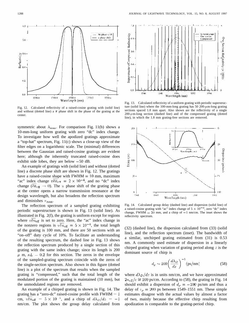
The reflection spectrum of a sampled grating exhibitingperiodic superstructure is shown in Fig. 13 (solid line). Asillustrated in Fig. 2(f), the grating is uniform except for regionswhere is set to zero. Here, the “ac” index change inthe nonzero regions is , the total lengthof the grating is 100 mm, and there are 50 sections with an“on–off” duty cycle of 10%. To facilitate an understandingof the resulting spectrum, the dashed line in Fig. 13 showsthe reflection spectrum produced by a single section of thisgrating with the same index change; since its length is 200

m, for this section. The zeros in the envelopeof the sampled-grating spectrum coincide with the zeros ofthe single-section spectrum. Also shown in this figure (dottedline) is a plot of the spectrum that results when the sampledgrating is “compressed,” such that the total length of themodulated portion of the grating is maintained (10 mm), butthe unmodulated regions are removed.

An example of a chirped grating is shown in Fig. 14. Thegrating has a “zero-dc” raised-cosine profile with FWHMcm, , and a chirp ofnm/cm. The plot shows the group delay calculated from

Fig. 13. Calculated reflectivity of a uniform grating with periodic superstruc-ture (solid line) where the 100-mm-long grating has 50 200-�m-long gratingsections spaced 1.8 mm apart. Also shown are the reflectivity of a single200-�m-long section (dashed line) and of the compressed grating (dottedline), in which the 1.8 mm grating-free sections are removed.

Fig. 14. Calculated group delay (dashed line) and dispersion (solid line) ofa raised-cosine grating with “ac” index change of 5� 10�4, zero “dc” indexchange, FWHM= 10 mm, and a chirp of�1 nm/cm. The inset shows thereflectivity spectrum.

(32) (dashed line), the dispersion calculated from (33) (solidline), and the reflection spectrum (inset). The bandwidth ofa similar, unchirped grating estimated from (31) is 0.53nm. A commonly used estimate of dispersion in a linearlychirped grating when variation of grating period alongis thedominant source of chirp is

ps nm (58)

where is in units nm/cm, and we have approximatedps/cm. According to (58), the grating in Fig. 14

should exhibit a dispersion of ps/nm and thus adelay of ps between 1549–1551 nm. These simpleestimates disagree with the actual values by almost a factorof two, mainly because the effective chirp resulting fromapodization is comparable to the grating-period chirp.

ERDOGAN: FIBER GRATING SPECTRA 1289

Fig. 15. Calculated bar transmissiont= through a uniform grating (solidline), a Gaussian grating (dashed line), and a chirped Gaussian grating (dottedline) with grating parameters given in the text.

Several examples of bar-transmission spectra throughnonuniform transmission gratings are shown in Fig. 15. Thesolid line shows transmission through a uniform grating witha coupling-length product of , “zero-dc” indexchange ( ), an effective-index difference of

, and a length of 10 cm. The dashed line representsthe transmission through a similar grating but with a Gaussianprofile where the coupling-length product has been slightlyreduced to FWHM to maintain maximum coupling.Note the reduction of the side lobes, just as occurs for Bragggratings. Although no example is shown, if the “dc” indexchange were nonzero, as shown in Fig. 2(b), the Gaussiangrating spectrum would exhibit “Fabry–Perot” structure on theshort-wavelength side of the spectrum similar to that shownin Fig. 10. The dotted line in Fig. 15 is the transmissionspectrum obtained for a similar Gaussian grating with a linearchirp of nm/cm and FWHM .Fig. 16 shows the spectrum of the group delay and dispersionassociated with this grating; the cross transmission is shownin the inset. Although the dispersion is relatively small for thisexample, note how linear the delay is over the full bandwidthof the grating.

IV. TILTED GRATINGS

Another parameter the designer of fiber gratings has at hisdisposal is the tilt of the grating fringes in the core of the fiber[29], [30]. The main effect of grating tilt in a single-modeBragg grating is to effectively reduce the fringe visibilitydefined in (1), (13), and (14). However, grating tilt can alsodramatically affect the coupling to radiation modes, whichwe discuss briefly in Section VI, as well as enable otherwiseunallowed coupling between discrete bound modes of fiber.The latter interaction has been demonstrated in both Bragg[31] and transmission gratings [32] that couple the LP01 modeto the LP11 mode of a dual-mode fiber.

To see how grating tilt affects single-mode Bragg reflectionin a fiber grating, suppose that the induced index change in the

Fig. 16. Group delay and dispersion for the cross amplitude of light trans-mitted through the chirped Gaussian grating described in Fig. 15. Crosstransmissiont� is shown in the inset.

Fig. 17. Diagram of the parameters associated with a tilted phase grating inthe core of an optical fiber.

core of the fiber is rotated by an angle, such that it is

(59)

where the -axis, shown in Fig. 17, is defined to be. The grating period along the(fiber) axis,

which determines the resonant wavelengths for coupling, isthus . For the slowly varying functionsand , we take ; i.e., we simply take theprojection of these functions onto the fiber axis. The generalcoupling coefficient in (14) then becomes

(60)

where we recognize that the subscriptsand describe thesame mode, except when one is associated with the forward-going mode ( ) the other describes the backward-going mode( ). The self and cross coupling coefficients now become

(61)

and

(62)

1290 JOURNAL OF LIGHTWAVE TECHNOLOGY, VOL. 15, NO. 8, AUGUST 1997

Fig. 18. Plot of the normalized effective fringe visibility associated withsingle-mode Bragg reflection in a tilted grating in the core of a fiber withparameters described in the text.

Notice that . Except for scaling of the slowlyvarying functions, the effects of tilt can be lumped into an“effective fringe visibility” , defined such that

(63)

Therefore, we may write

(64)

in direct analogy to (13). This important result states that theeffect of grating tilt on single-mode Bragg reflection is simplyto reduce the effective fringe visibility by an amount given in(63). As an example, Fig. 18 shows a plot of the normalizedeffective fringe visibility as a function of tilt angle for theLP01 mode in a fiber with a cladding index of 1.44, a core-cladding , a core radius of m, and ata wavelength of 1550 nm.

The Bragg reflection spectrum for a tilted grating can stillbe calculated from (15) and (16) where now .Fig. 19 shows reflection spectra over a range of tilt anglesfor a Gaussian grating with a FWHM mm, a maximumindex change of , and zero-tilt visibility

. Because tilt affects Bragg reflection by effectivelyreducing the fringe visibility, this plot also demonstrates howthe reflection spectrum of a Gaussian grating changes as thevisibility is reduced (here by keeping the “dc” index changeconstant). Proper use of tilt for reducing the effective visibilityand hence, Bragg reflection can be practically useful in caseswhere large radiation or other bound mode coupling is desiredbut Bragg reflection is undesirable [31].

Fig. 19. Calculated reflectivity spectrum over a range of grating tilt anglesfor a Gaussian grating.

V. COUPLING TO CLADDING MODES

There are numerous applications of fiber gratings that in-volve coupling of light into and out of the core mode(s) ofa fiber. Fig. 20 shows measured spectra of the transmissionof an LP core mode through an untilted Gaussian fibergrating that is 5 mm long and has a maximum index changeof . In Fig. 20(a) the bare (uncoated)section of fiber that contains the grating is immersed inindex-matching fluid to simulate an infinite cladding. Whatresults is a smooth transmission profile for nmdemonstrating loss due to coupling of the core mode to thecontinuum of radiation modes. Radiation mode coupling isbriefly discussed in Section VI and is described in detailin [28] and [29]. In Fig. 20(b), the fiber is immersed inglycerin, which has a refractive index greater than the claddingindex. The transmission spectrum now exhibits fringes that arecaused by Fabry–Perot-like interference resulting from partialreflection of the radiation modes off of the cladding–glycerininterface. In Fig. 20(c) the bare fiber is surrounded by air;for the wavelengths shown in this plot, the LP01 core modecouples into distinct backward-going cladding modes with awell-defined resonance peak for each mode. Here we brieflyexamine this last type of interaction. A more detailed descrip-tion can be found in [33].

Fig. 4(b) illustrates coupling of a core mode to a claddingmode from a ray point-of-view, where cladding modes arebound modes of the total fiber with (assumingthe fiber is surrounded by air). It is shown above that thegrating period required for co-propagating coupling between acore mode of index and a cladding mode of index is

. In analogous fashion, counter-propagatingmodes [ in Fig. 4(b)] can be coupled by a grating witha much shorter period .

Using the coupled-mode theory outlined above, the equa-tions that describe coupling among the LP01 core mode andthe (exact) cladding modes of order 1by a reflection grating

ERDOGAN: FIBER GRATING SPECTRA 1291

(a)

(b)

(c)

Fig. 20. Measured transmission through a Bragg grating where (a) theuncoated fiber is immersed in index-matching liquid to simulate an infinitecladding, (b) the fiber is immersed in glycerin, and (c) the bare fiber issurrounded by air and thus supports cladding modes.

are [33]

––

––

––

(65)

––

–– (66)

where the detuning is

–– (67)

Here, –– is the self-coupling coefficient for the LP01

mode given by (19), –– is the cross-coupling coefficient

defined through (12) and (13), and we have neglected termsthat involve self and cross coupling between cladding modessince the associated coupling coefficients are very small, or

––

––

––

–– . In (65) and (66), we

have also not included Bragg reflection of the LP01 core mode,making these equations valid only at wavelengths far awayfrom this Bragg resonance.

(a)

(b)

Fig. 21. (a) Measured and (b) calculated transmission through a strongGaussian Bragg grating, showing both core-mode Bragg reflection intocladding modes.

The common synchronous approximation was used in ob-taining (65) and (66), but unlike (15) and (16) the resultingequations contain coefficients that oscillate rapidly along.This is because there are now multiple values of, whichare not easily removed by defining and as we did for(15) and (16). However, if the cladding mode resonances donot overlap, then we may calculate each resonance separately,retaining only the core mode and the appropriate claddingmode for the resonance. In that case, the problem reduces tosimple two-mode coupling, as described in detail in Sections IIand III.

As an example of cladding-mode coupling in a Bragggrating, Fig. 21 shows the measured (a) and calculated (b)transmission spectrum through a Gaussian grating written inhydrogen-loaded [34] Corning Flexcore fiber. The gratinglength is FWHM mm, the index change is

, and the visibility is approximately . Thelarge transmission dip at 1541 nm is the Bragg reflection reso-nance, while the remaining dips are cladding mode resonances.Here the resonances overlap substantially over most of thewavelength range shown in the plot. As a result, an accuratecalculation could be obtained only by including multiple (butnot necessarily all) cladding modes in (65) and (66) at eachwavelength. The resolution in the experimental measurementis 0.1 nm.

The equations that describe coupling among the LP01 coremode and the cladding modes of order 1by a transmission

1292 JOURNAL OF LIGHTWAVE TECHNOLOGY, VOL. 15, NO. 8, AUGUST 1997

(a)

(b)

Fig. 22. Calculated transmission spectra through (a) a relatively weak and(b) a stronger transmission grating, each designed to couple the LP01 coremode to the� = 7 cladding mode at 1550 nm. Solid lines represent a uniformgrating while the dashed line represents a Gaussian grating.

grating are [33]

––

––

––

(68)

––

–– (69)

–– (70)

In arriving at (68) and (69), approximations were appliedsimilar to those made for (65) and (66). Fig. 22 shows calcu-lated examples of cladding-mode coupling in a transmissiongrating. Fig. 22(a) shows the transmission for a relatively weakgrating with a length (FWHM) of 25 mm, a maximum indexchange of , and a uniform (solid line) orGaussian (dashed line) profile. The four main dips seen inthese spectra correspond to coupling to the , , ,

, and cladding modes. Fig. 22(b) shows the transmissionfor a stronger, uniform grating with an induced index changeof 1 10 3. In each case the grating period is adjusted toachieve coupling at 1550 nm between the LP01 core mode andthe cladding mode. That is, the gratings in Fig. 22(a)and (b) have periods of m and m,respectively.

In the above discussion we consider only thecladdingmodes with azimuthal order . In an untilted gratingcoupling may occur only between modes of the same az-imuthal symmetry (as shared by the LP01 HE11 modeand the exact HE/EH cladding modes). In a typical 125-

m diameter fiber there are several hundred claddingmodes at IR communications wavelengths. In a tilted grating,in which coupling to an enormous number of higher azimuthal-order cladding modes is allowed, the resonances are so denselyspaced that they are generally not well resolvable.

VI. RADIATION -MODE COUPLING

Although numerous applications are possible for fiber grat-ings as waveguide-grating couplers that couple free-spacebeams into and out of bound fiber modes, surprisingly littlework has been reported in this area. However, the effect ofradiation-mode coupling as a loss mechanism on core-modetransmission has been studied [28], [29]. We do not describethis situation in detail, but merely introduce the reader tothe main concepts in order to put radiation-mode couplingin context with the interactions discussed above.

Fig. 23 illustrates the coupling of an LP01 core mode to thecontinuum of backward propagating radiation modes from aray point of view. The coupling strength to these high-order(small- ) modes is quite small unless the grating is suitablyblazed. But as Fig. 20(a) illustrates, if the fiber is immersed inan index matching fluid or recoated with a high-index polymer,bound cladding modes cease to exist and substantial couplingto low-order ( ) radiation modes can occur near theBragg reflection resonance even in untilted gratings. A usefulquantity to be aware of is the wavelength at which trueradiation-mode (not cladding-mode) coupling “cuts” on and/oroff. Assuming the core confinement factor for the radiationmodes is much smaller than that of the bound mode of interest,then we find

(71)

where for the case of an infinitely clad fiber with index[see Fig. 20(a)], or when the fiber is surrounded by

air such that bound cladding modes may propagate. The “”sign in the first factor applies to reflection, while the “” signcorresponds to forward coupling. The second factor describesthe shift of with increasing “dc” index change.

Consider the coupling of an LP01 core mode to backward-propagating radiation modes labeled LP, where the discreteindex identifies the polarization and azimuthal order, while

the continuous label denotes thetransverse wavenumber of the radiation mode (is theusual axial propagation constant). Here we assume the fiberhas a cladding of index and with an infinite radius. Thecoupled-mode equations for this case are then

––

––

–– (72)

––

–– (73)

ERDOGAN: FIBER GRATING SPECTRA 1293

Fig. 23. Ray-optic illustration of core-mode coupling to abackward-traveling radiation mode by a Bragg grating. The� axesbelow the diagram demonstrates the grating condition in (5) form� 1.

where

–– (74)

and where is the amplitude of the core mode, are theamplitudes of the (continuous spectrum of) radiation modes,and the usual summation now includes an integral in (72).Also, –

– is the LP self-coupling coefficient given by(19), and –

––– is the cross-coupling coefficient

defined through (12) and (13). By applying essentially a “firstBorn approximation” to the core-mode amplitude, we canobtain an approximate expression for from (73). Afterinserting this result into (72) and performing the integral over

, it can be shown [28], [29] that the core mode amplitudeapproximately obeys an equation of the form

––

–– (75)

where the term in square brackets is evaluated at. Since this term is real, clearly it gives rise to

exponential loss in the amplitude of the core mode. Noticethe loss coefficient is proportional to the square of the cross-coupling coefficient, and hence, to the square of the inducedindex change.

Although the analysis given here is simplified, it is possibleto predict the radiation-mode coupling loss spectrum evenwhen the grating is tilted following a similar developmentto that in Section IV. As might be expected, as the tiltangle is increased (the grating is blazed), light can be cou-pled more efficiently at smaller angles . But increasinglymany radiation-mode azimuthal orders must be included inthe summation in (75) to accurately model radiation modespropagating more normal to the fiber axis. As an example ofsome typical transmission spectra, Fig. 24 shows a calculationof the loss in transmission through the same Gaussian gratingdescribed in Fig. 19, only here . Spectraare shown for a range of tilt angles between 0 –45, wherethe grating period along the fiber axis is kept constant. TheLP01 mode incident on the grating is assumed to be polarizedperpendicular to both the and axes (see Fig. 17). The

Fig. 24. Calculated loss in transmission through a Gaussian grating in a fiberwith an infinite cladding over a range of grating tilt angles.

peak at the longest wavelength results from Bragg reflection,whereas the loss at other wavelengths is due to radiation-modecoupling. As expected, the efficiency for coupling to smallerand smaller angles (which occurs at shorter wavelengths)improves as the grating is increasingly blazed.

VII. CONCLUSIONS

We have presented principles and tools for understanding thespectra exhibited by fiber Bragg and transmission gratings. Itis hoped that the reader less familiar with these exciting com-ponents now has a base with which to understand the currentand potential applications of fiber gratings, and that the moreexperienced reader has benefited from a concise description ofmultiple fiber-grating phenomena with a uniform notation.

An important principle to take away from Section II is thatthe simple closed-form expressions for optical properties ofuniform fiber gratings are frequently excellent approximationsfor nonuniform gratings as well. This section also uncoverssome of the basic similarities and differences between Bragggratings and transmission gratings. One important differenceis that as a Bragg grating is made increasingly stronger (byenlarging ), the maximum reflectivity and bandwidthsimply increase; in contrast, to obtain a strong resonance in atransmission grating requires hitting a “target” (usually

) to avoid over-coupling.By examining nonuniform gratings in Section III, we found

that it is critical to take into account both apodization andchirp of the grating period when the dispersive characteristicsof fiber gratings are important. We also saw that it is almostalways advantageous to minimize the “dc” apodization, unlessit is intentionally utilized for tailoring dispersion, for example.In Section IV, we found that tilted gratings enable couplingbetween modes that have dissimilar azimuthal symmetry, andthat the effect of tilt on single-mode Bragg reflection can beregarded simply as a reduction in the effective fringe visibilityof the phase grating. Finally, in Sections V and VI, we brieflyexplored coupling from a core mode to cladding and radiationmodes. Although long-period cladding-mode coupling gratingshave recently seen rapid development [35], there appears tobe relatively little investigation into the apparently abundantpossibilities for applications based on exchange of light in thecore of a single-mode fiber with the readily accessible claddingand radiation modes.

1294 JOURNAL OF LIGHTWAVE TECHNOLOGY, VOL. 15, NO. 8, AUGUST 1997

ACKNOWLEDGMENT

The author would like to thank the Editors of this SpecialSection for the invitation to present this paper and the refereesfor their helpful comments.

REFERENCES

[1] K. O. Hill, B. Malo, F. Bilodeau, and D. C. Johnson, “Photosensitivityin optical fibers,”Annu. Rev. Mater. Sci.,vol. 23, pp. 125–157, 1993.

[2] W. W. Morey, G. A. Ball, and G. Meltz, “Photoinduced Bragg gratingsin optical fibers,”Opt. Photon. News,vol. 5, pp. 8–14, 1994.

[3] R. J. Campbell and R. Kashyap, “The properties and applications ofphotosensitive germanosilicate fiber,”Int. J. Optoelectron.,vol. 9, pp.33–57, 1994.

[4] P. St. J. Russell, J.-L. Archambault, and L. Reekie, “Fiber gratings,”Phys. World,pp. 41–46, Oct. 1993.

[5] I. Bennion, J. A. R. Williams, L. Zhang, K. Sugden, and N. J. Doran,“UV-written in-fiber Bragg gratings,”Opt. Quantum Electron.,vol. 28,pp. 93–135, 1996.

[6] Invited Papers,J. Lightwave Technol., this issue.[7] C. M. de Sterke, N. G. R. Broderick, B. J. Eggleton, and M. J.

Steel, “Nonlinear optics in fiber gratings,”Opt. Fiber Tech.,vol. 2, pp.253–268, 1996.

[8] D. Marcuse, Theory of Dielectric Optical Waveguides.New York:Academic, 1991, ch. 2.

[9] M. Born and E. Wolf, Principles of Optics. New York: Pergamon,1987, sec. 8.6.1, eq. (8).

[10] A. Yariv, “Coupled-mode theory for guided-wave optics,”IEEE J.Quantum Electron.,vol. QE-9, pp. 919–933, 1973.

[11] H. Kogelnik, “Theory of optical waveguides,” inGuided-Wave Opto-electronics,T. Tamir, Ed. New York: Springer-Verlag, 1990.

[12] J. E. Sipe, L. Poladian, and C. M. de Sterke, “Propagation throughnonuniform grating structures,”J. Opt. Soc. Amer. A,vol. 11, pp.1307–1320, 1994.

[13] H. Kogelnik, “Filter response of nonuniform almost-periodic structures,”Bell Sys. Tech. J.,vol. 55, pp. 109–126, 1976.

[14] K. O. Hill, “Aperiodic distributed-parameter waveguides for integratedoptics,” Appl. Opt.,vol. 13, pp. 1853–1856, 1974.

[15] B. Malo, S. Theriault, D. C. Johnson, F. Bilodeau, J. Albert, and K. O.Hill, “Apodised in-fiber Bragg grating reflectors photoimprinted usinga phase mask,”Electron. Lett.,vol. 31, pp. 223–225, 1995.

[16] F. Ouellette, “Dispersion cancellation using linearly chirped Bragggrating filters in optical waveguides,”Opt. Lett.,vol. 12, pp. 847–849,1987.

[17] M. E. Fermann, K. Sugden, and I. Bennion, “High-power soliton fiberlaser based on pulse width control with chirped fiber Bragg gratings,”Opt. Lett.,vol. 20, pp. 172–174, 1995.

[18] P. A. Morton, V. Mizrahi, T. Tanbun-Ek, R. A. Logan, P. J. Lemaire,H. M. Presby, T. Erdogan, S. L. Woodward, J. E. Sipe, M. R. Phillips,A. M. Sergent, and K. W. Wecht, “Stable single mode hybrid laserwith high power and narrow linewidth,”Appl. Phys. Lett.,vol. 64, pp.2634–2636, 1994.

[19] P. A. Morton, V. Mizrahi, P. A. Andrekson, T. Tanbun-Ek, R. A. Logan,P. Lemaire, D. L. Coblentz, A. M. Sergent, K. W. Wecht, and P. F.Sciortino, Jr., “Mode-locked hybrid soliton pulse source with extremelywide operating frequency range,”IEEE. Photon. Technol. Lett.,vol. 5,pp. 28–31, 1993.

[20] H. A. Haus and C. V. Shank, “Antisymmetric taper of distributed-feedback lasers,”IEEE J. Quantum Electron.,vol. QE-12, pp. 532–539,1976.

[21] W. H. Loh and R. I. Laming, “1.55�m phase-shifted distributedfeedback fiber laser,”Electron. Lett.,vol. 31, pp. 1440–1442, 1995.

[22] B. J. Eggleton, P. A. Krug, L. Poladian, and F. Ouellette, “Long periodicsuperstructure Bragg gratings in optical fibers,”Electron. Lett.,vol. 30,pp. 1620–1622, 1994.

[23] J. Martin, M. Tetu, C. Latrasse, A. Bellemare, and M. A. Duguay,“Use of a sampled Bragg grating as an in-fiber optical resonator forthe realization of a referencing optical frequency scale for WDMcommunications,” inOptical Fiber Communications Conf.,Dallas, TX,Feb. 16–21, 1997, paper ThJ5.

[24] R. Kashyap, H.-G. Froehlich, A. Swanton, and D. J. Armes, “1.3 mlong super-step-chirped fiber Bragg grating with a continuous delay of13.5 ns and bandwidth 10 nm for broadband dispersion compensation,”Electron. Lett.,vol. 32, pp. 1807–1809, 1996.

[25] L. Dong, M. J. Cole, M. Durkin, M. Ibsen, and R. I. Laming, “40Gbit/s 1.55�m transmission over 109 km of nondispersion shifted fiberwith long continuously chirped fiber gratings,” inOptic. Fiber Commun.Conf., Dallas, TX, Feb. 16–21, 1997, paper PD6.

[26] L. A. Weller-Brophy, “Analysis of waveguide gratings: Application ofRouard’s method,”J. Opt. Soc. Amer. A,vol. 2, pp. 863–871, 1985.

[27] M. Yamada and K. Sakuda, “Analysis of almost-periodic distributedfeedback slab waveguides via a fundamental matrix approach,”Appl.Opt., vol. 26, pp. 3474–3478, 1987.

[28] V. Mizrahi and J. E. Sipe, “Optical properties of photosensitive fiberphase gratings,”J. Lightwave Technol.,vol. 11, pp. 1513–1517, 1993.

[29] T. Erdogan and J. E. Sipe, “Tilted fiber phase gratings,”J. Opt. Soc.Amer. A,vol. 13, pp. 296–313, 1996.

[30] R. Kashyap, R. Wyatt, and R. J. Campbell, “Wideband gain flattenederbium fiber amplifier using a photosensitive fiber blazed grating,”Electron. Lett.,vol. 29, pp. 154–156, 1993.

[31] T. A. Strasser, J. R. Pedrazzani, and M. J. Andrejco, “Reflective modeconversion with UV-induced phase gratings in two-mode fiber,” inOptic. Fiber Commun. Conf.,Dallas, TX, Feb. 16–21, 1997, paper FB3.

[32] K. O. Hill, B. Malo, K. A. Vineberg, F. Bilodeau, D. C. Johnson, and I.Skinner, “Efficient mode conversion in telecommunication fiber usingexternally written gratings,”Electron. Lett.,vol. 26, pp. 1270–1272,1990.

[33] T. Erdogan, “Cladding-mode resonances in short and long period fibergrating filters,”J. Opt. Soc. Amer. A,vol. 14, no. 8, Aug. 1997.

[34] P. J. Lemaire, R. M. Atkins, V. Mizrahi, K. L. Walker, K. S. Kranz, andW. A. Reed, “High pressure H2 loading as a technique for achievingultrahigh UV photosensitivity and thermal sensitivity in GeO2 dopedoptical fibers,”Electron. Lett.,vol. 29, pp. 1191–1193, 1993.

[35] A. M. Vengsarkar, P. J. Lemaire, J. B. Judkins, V. Bhatia, T. Erdogan,and J. E. Sipe, “Long-period fiber gratings as band-rejection filters,”J.Lightwave Technol.,vol. 14, pp. 58–65, 1996.

Turan Erdogan (S’90–M’92) received the B.S. de-grees in physics and electrical engineering from theMassachusetts Institute of Technology, Cambridge,in 1987, and the Ph.D. degree from The Institute ofOptics at the University of Rochester, Rochester,NY, in 1992. His doctoral research focused onnovel approaches to surface-emitting semiconductorlasers, including concentric-circle-grating surface-emitting lasers, and optical physics of diffractiongratings and cavities.

Until 1994, he was with AT&T Bell Laboratoriesin Murray Hill, NJ, where he conducted research and development of fibergrating-based devices for advanced optical communications systems. In 1994,he joined the Faculty of The Institute of Optics, Rochester, NY, as an AssistantProfessor, where he continues to conduct research on fiber and semiconductordevices, including fiber gratings.

Dr. Erdogan is an Alfred P. Sloan Research Fellow, a recipient of an NSFFaculty Early Career Development (CAREER) Award, and winner of the 1995Adolph Lomb Medal of the Optical Society of America.