FIELD EXPERIMENTAL STUDY OF THE SMAGORINSKY MODEL AND APPLICATION TO LARGE EDDY SIMULATION by Jan Kleissl A dissertation submitted to The Johns Hopkins University in conformity with the requirements for the degree of Doctor of Philosophy in Environmental Engineering Baltimore, Maryland January 2004 c Copyright by Jan Kleissl 2004
Transcript
FIELD EXPERIMENTAL STUDY OF
THE SMAGORINSKY MODEL AND
APPLICATION TO LARGE EDDY
SIMULATION
by
Jan Kleissl
A dissertation submitted to The Johns Hopkins University in
conformity with the requirements for the degree of
term in the rotational form (Orszag and Pao 1974). Finally, the viscous term is neglected which
can be justified in these high Reynolds number flows. Now Eq. 1.8 becomes
∂tui + uj (∂j ui − ∂iuj) = −∂ip∗ + fi − gθ′
θ0δi3 − ∂jτ
dij (1.11)
For more details on the derivation see Galperin and Orszag (1993). In LES, one must model
the SGS stresses τdij , which are three-dimensional, time-dependent, turbulent fields with stochastic
character and display a number of interesting statistical properties (for a review, see Meneveau and
Katz 2000). Different models for τij will be discussed in the next chapter.
1.3 Eddy viscosity subgrid-scale models and energy dissipation
The realism of the SGS model is essential for the ability of LES to provide realistic turbulent fields
in the ABL, especially in regions close to the lower boundary. There the local integral scale is on
the order of the distance from the boundary, z, and thus ∆/z > 1. Hence, the SGS model must
represent the momentum fluxes carried by most of the eddies, even the large, energy-containing
ones. The most commonly employed parameterization for the SGS stress is the Smagorinsky model
(Smagorinsky 1963):
τSmagij − 1
3τkkδij = −2νT Sij , νT = (cs∆)
2∣∣∣S
∣∣∣ . (1.12)
Sij = 0.5 (∂ui/∂xj + ∂uj/∂xi) is the strain rate tensor and∣∣∣S
∣∣∣ =√
2SijSij is its magnitude, νT is
the eddy viscosity, and cs is the Smagorinsky coefficient, which in traditional LES is prescribed based
on phenomenological theories of turbulence or adjusted empirically. The product of Smagorinsky
6
coefficient and filter scale is a mixing-length often denoted by l = ∆cs. For a recent review of the
Smagorinsky model and other SGS models see Meneveau and Katz (2000). As also discussed in
this review, the magnitude of cs determines the effectiveness with which kinetic energy is dissipated
out of the resolved velocity field during LES. The mean rate of kinetic energy transfer from the
resolved to the subgrid range of scales (the so-called SGS dissipation) is given by
〈Πmeas〉 = −〈τijSij〉, (1.13)
where 〈〉 denotes ensemble or time averaging, depending on the context. The rate that results from
replacing τij with the Smagorinsky model is given by
〈ΠSmag〉 = 2 (cs∆)2 〈
∣∣∣S∣∣∣ SijSij〉. (1.14)
By requiring that 〈Πmeas〉 = ǫ = 〈ΠSmag〉 (where ǫ is the molecular dissipation rate), Lilly (1967)
analytically derives a value of cs of approximately 0.16 - 0.20 (the exact value depends on the filter
shape and the Kolmogorov constant). His main assumption is the application of a filter operation
at a scale ∆ that falls within an idealized inertial subrange of turbulence with energy spectrum
E(k) = αǫ2/3k−5/3 to evaluate 〈∣∣∣S
∣∣∣ SijSij〉. This derived value of cs exceeds significantly what LES
calculations require to yield realistic results, especially close to the ground (Deardorff 1970; Moin
and Kim 1982; Mason and Thomson 1992; Sullivan et al. 1994). As is widely recognized, near the
ground ∆ approaches or exceeds energy containing scales and hence the basic assumption of Lilly
(1967) breaks down.
Wall-blocking effects are known to cause a reduction in the coefficient when approaching the
ground. Mason (1994) proposes to match the basic mixing length of the Smagorinsky model in
the interior of the ABL, l0 = c0∆, with rough-surface expressions for the eddy viscosity νT =
7
κ2 (z + z0)2∂〈u〉/∂z near the ground. Mason’s (1994) modified mixing length l reads:
l =
(1
[κ(z + z0)]n +
1
ln0
)−1/n
. (1.15)
Thermal stratification also influences the SGS energy spectrum of turbulence, which in turn
violates Lilly’s assumption of a long inertial subrange in deriving cs. In particular, the coefficient
has to be decreased in stably stratified conditions. This trend is reflected in Deardorff’s (1980)
empirical model, as well as in the model of Brown et al. (1994), who derive a stability-dependent
model from the SGS energy equation assuming a state of local equilibrium. Canuto and Cheng
(1997) employ a two-point closure to construct the SGS energy spectrum under the influence of
shear and buoyancy. From the SGS energy spectrum they derive an analytical expression for the
reduction of cs under shear and buoyancy. Like stratification, the presence of mean shear also
requires decreasing the Smagorinsky coefficient.
Similarly to the filtered momentum equations, the filtered scalar transport equations (e.g. heat
equation) in LES include an additional term, the SGS scalar flux. The SGS heat flux is defined
according to
qi = θui − θui, (1.16)
where θ is the temperature field. In the Smagorinsky, or eddy-diffusivity model, qi is parameterized
as
qSmagi = −Pr−1
T c2s∆
2∣∣∣S
∣∣∣ ∂θ′
∂xi, (1.17)
where PrT is the turbulent SGS Prandtl number, and θ is the filtered temperature field. The prime
indicates fluctuating quantities around the average (θ = 〈θ〉 + θ′). The mean SGS dissipation of
scalar variance 〈χmeas〉 is usually defined as
〈χmeas〉 = −〈qi∂θ′
∂xi〉. (1.18)
8
Lilly’s analysis applied to a scalar variance spectrum in isotropic, neutral turbulence led to an
estimate of the Prandtl number of about 0.5 for the Smagorinsky model (Mason 1994). Laboratory
experimental investigations in the wake of a heated cylinder (Kang and Meneveau 2002) resulted
in PrT ≈ 0.3. As part of the present study we will also examine how Pr−1T c2
s (and PrT ) depend on
distance to the ground, flow stability, and averaging time-scale.
It is worthwhile to delineate that in this dissertation we restrict our attention to the basic
structure of the eddy-viscosity Smagorinsky closure. This closure is based on the assumption
that the SGS stresses and fluxes are aligned to the gradients of velocity and temperature. The
drawbacks of this assumption have already been documented extensively in the literature: As
reviewed in Meneveau and Katz (2000) and Tao et al. (2002) in the context of experimental
studies in laboratory turbulence, the alignment hypothesis is not accurate. In the context of ABL
turbulence, Higgins et al. (2003, 2004) confirm this limitation and show that addition of a so-called
tensor eddy-diffusion model improves the alignment trends. Moreover, near the ground, Tong et
al. (1999) show that the streamwise accelerations inherent in the eddy-viscosity closures cause
unphysical couplings with the resolved velocity field. Moreover, Mason and Thomson (1992) argue
that the SGS models must represent stochastic fluctuations of the unresolved stresses. Even with
these limitations, the deterministic eddy-viscosity closure is still the most-often used in practical
applications, providing continued interest in the dependence of cs on physical flow parameters as
studied here.
1.4 Experiments for the evaluation of subgrid-scale quantities
In order to determine subgrid-scale (SGS) quantities such as τij , Sij , and cs in field experiments,
velocity fields need to be filtered in three dimensions in space (Eq. 1.3). Theoretical and compu-
tational analysis has shown that 2d filtering is a good approximation to 3d filtering. Tong et al.
(1998) estimate that near the surface 2d filtering “removes wavenumber modes that contribute to
more than 85% of variance of the SGS fluctuations”. They demonstrate from high resolution LES
9
data that 2d and 3d filtered fields are indistinguishable. From DNS data of turbulent channel flow,
Murray et al. 1996 obtain a criterion of y+ > 10 for the equivalence of 2d and 3d filtering. Specifi-
cally designed field experiments with horizontal arrays of high frequency sensors in the atmospheric
boundary layer enable the SGS physics to be studied from variables filtered in 2d horizontal planes
using Taylor’s hypothesis. In the vertical direction, typically only two heights are sampled. This
resolution is not sufficient for filtering. As reviewed in Meneveau & Katz (2000), there also exist
measurement techniques that do not require Taylor’s hypothesis. Particle Image Velocimetry (PIV)
has been used in engineering flows. In atmospheric sciences radar and LIDAR (light detection and
ranging) are being developed to get 3d information on the flow. These techniques still face many
drawbacks and do not permit the necessary high resolution for turbulence measurements (ideally
∼ 3 × 10³ Hz ∼ Uc/η, where Uc is the turbulence convection velocity). In experiments analyzed
in this thesis, 3d sonic anemometers are deployed, which are able to measure all three components
of the velocity vector and the potential temperature. The sampling rate is up to 60 Hz, which is
sufficient to resolve the energy containing scales and significant portions of the inertial range.
In the context of LES of the atmospheric boundary layer, a number of field studies have aimed
at measuring qi and τij from field data and at analyzing the results to improve SGS modelling. A
study using data from a single 3d-sonic anemometer (Porte-Agel et al. 1998) restricted the analysis
to 1d filtering (time-filtering and interpreting the results as spatial filtering in the x1 = x direction
using Taylor’s hypothesis). Tong et al. (1998) proposed deploying a horizontal array of sensors
and examined filtering issues using LES data. Their results showed that filtering in two horizontal
directions was required for quantitatively more accurate results. Experimental results from one
horizontal array of sensors using 2d filtering were reported in Tong et al. (1999), and Porte-Agel et
al. (2000a). The latter paper showed that while filter dimensionality did not have a strong effect
on the previously reported trends based on 1d filtering, atmospheric stability had strong effects on
the results. Limiting the setup of Porte-Agel et al. (2000a) was the inability to compute vertical
derivatives. This issue was addressed by using two vertically displaced horizontal arrays as proposed
in Tong et al. (1999), and also in the Davis 1999 experiment (Porte-Agel et al. 2001a). As described
10
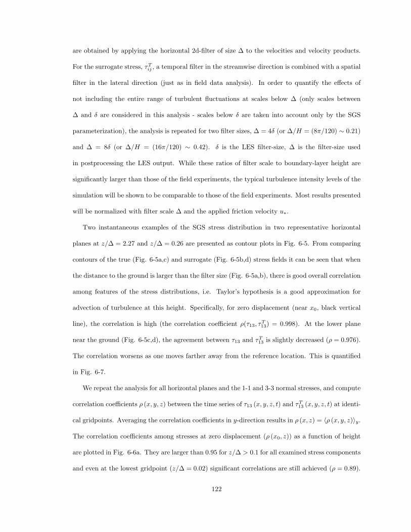
Figure 1-1: Photograph of the setup of array 1 during the HATS experiment near Kettlemen City,CA. Photo courtesy of Tom Horst, NCAR.
in chapter 2.2, a similar setup is used in the Horizontal Array Turbulence Study (HATS, Fig. 1-1)
now including two more anemometers, and including more data under stable stratification, due to
prevailing wind conditions at night.
In order to become familiar with measured physical quantities and scales of motion in these
experiments it is instructive to look at the data in horizontal planes (Fig. 1-2 for the HATS
experiment). In the x direction there are nine data points (nine sonics) for the lower height (zd =
3.45 m). The time series of all sonics are plotted in the y direction. A correlation between u3 and
θ is observed. In this unstable situation (daytime) hot air from the ground is transported upwards,
while colder air from above is mixed down to the ground. In addition there is an anti-correlation
between u1 and u3, which follows from mass continuity. From this type of data the SGS stresses and
their model predictions can be obtained experimentally by filtering the signals and by appropriate
post-processing, in order to address the research questions outlined in the section below.
11
Figure 1-2: Horizontal contour plots of streamwise velocity, vertical velocity, and temperature atzd = 3.45 m on September 6, 2000, 1603h PST in Kettlemen City, CA.
1.5 Research Questions
This dissertation addresses research questions related to SGS modeling in LES. In particular, the
Smagorinsky coefficient is measured from atmospheric field data and a priori and a posteriori tests of
dynamic SGS models are performed. An a priori test “uses experimental or DNS data to measure
directly the accuracy of a modeling assumption, for example, the relation for the residual-stress
tensor (...) given by the Smagorinsky model” (Pope 2000, p. 601). In a posteriori tests, “the model
is used to perform a calculation for a turbulent flow, and the accuracy of calculated statistics (e.g.
〈U〉 (...)) is assessed, again by reference to experimental or DNS data. It is natural and appropriate
to perform a priori tests to assess directly the validity and accuracy of approximations being made.
12
However, for the LES approach to be useful, it is success in a posteriori tests that is needed.” (Pope
2000, p.601). Through this research the following questions are addressed:
• Can SGS model coefficients be measured accurately from field measurements with horizontal
arrays of sonic anemometers in the atmospheric surface layer?
• Which turbulence length scales does cs depend on? Investigators have proposed that cs
decreases in stable conditions and near the surface (Deardorff 1980, Brown et al. 1994,
Canuto and Cheng 1997). Can these trends be confirmed and quantified from the field data?
• Do dynamic SGS models predict the correct cs under different flow conditions when tested
a priori in field experiments? It is known that the scale-invariance assumption in the classic
dynamic SGS model (Germano et al. 1991) causes an underprediction of cs near the wall.
Does the scale-dependent dynamic model (Porte-Agel et al. 2000b) improve the prediction?
• Is the prediction for cs of dynamic SGS models in LES similar to the results from the field
experiment? Do these SGS models improve turbulence properties such as non-dimensional
velocity gradients a posteriori?
• How does the coefficient of the eddy viscosity model for the SGS heat flux depend on turbu-
lence length scales?
1.6 Outline of the thesis
This thesis is organized as follows: Chapter 2 is dedicated to measuring and characterizing cs from
the field data. In chapter 2.2, the field experiment and the data set used in the present study
are described. Chapters 2.3 - 2.7 describe the results on the magnitude of the measured cs as
a function of atmospheric stability, distance to the ground, and local strain-rate magnitude. A
similar analysis for the SGS heat flux is also presented. In chapter 3 it is determined whether
the scale-invariant dynamic model and the scale-dependent dynamic model can predict the correct
cs under different stability conditions and heights. Chapter 4 presents the application of these
13
dynamic models to Large Eddy Simulation of atmospheric flow forced by a diurnal cycle of surface
heat flux. A summary and conclusions are presented in chapter 5.
14
Chapter 2
Magnitude and Variability of subgrid-scale
eddy-diffusion coefficients in the atmospheric
surface layer
2.1 Introduction
In this chapter we process data from field experiments using the horizontal array technique presented
briefly in chapter 1.4 to measure cs under flow conditions prevalent in the atmospheric surface
layer. In order to measure cs under flow conditions that are more general than the isotropic
conditions of Lilly’s (1967) original derivation, his theoretical approach can be applied to analysis
of experimental data by setting the dissipation from the Smagorinsky model equal to the real
measured SGS dissipation, i.e. by setting 〈Πmeas〉 = 〈ΠSmag〉. An empirically measurable SGS
dissipation-based Smagorinsky coefficient can thus be defined as follows:
c2s = − 〈τijSij〉
〈2∆2∣∣∣S
∣∣∣ SijSij〉. (2.1)
This approach was pioneered by Clark et al. (1979) for the analysis of data from Direct Numerical
Simulations (DNS). As reviewed in Meneveau and Katz (2000), since then many studies have used
15
this criterion to compute cs.
In this chapter we aim at deriving, from the field data, empirical relationships for cs as a function
of relevant parameters such as distance to the ground, strength of thermal stratification, and strain-
rate magnitude. The distance to the ground, z, can be normalized with the filter scale, ∆, yielding
the parameter ∆/z. Stratification can be characterized using the Obukhov length L, defined in Eq.
1.1. The dimensionless parameter comparing the filter scale to L is ∆/L. The local strain-rate will
be quantified by∣∣∣S
∣∣∣, the magnitude of the strain-rate tensor already defined in Eq. 1.12. It can be
normalized with a velocity scale and a length scale. The proper choice of velocity and length scales
depends on whether ∆ falls inside or outside the inertial range.
In addition to the dependence of cs on these parameters, the great variability of turbulence
dynamics in general, and of atmospheric dynamics in particular, raises the issue of how the averaging
procedures needed in evaluating terms in Eq. 2.1 should be performed, and how meaningful the
results are. Variability in cs is caused by the inherent intermittency of turbulence, and of ABL
flow patterns in particular. It is well known that the SGS dissipation Πmeas in turbulence is
highly intermittent. This was already shown for isotropic turbulence using DNS by Cerutti and
Meneveau (1998) and for the ABL in the context of the SGS dissipation of scalar variance by
previous experiments described in Porte-Agel et al. (2000a, 2001a, 2001b). To examine the effects
of intermittency upon eddy-viscosity coefficients, the averages in the numerator and denominator
of Eq. 2.1 can be computed over different time scales Tc. Then cs is no longer a single value but
fluctuates from one time-period (of length Tc) to another. We wish to examine how this variability
is affected by varying Tc under different flow conditions. Moreover, in LES using the Lagrangian
dynamic model (Meneveau et al. 1996), one needs to prescribe a time scale. This time scale is
used in that model to set the duration of averaging over the history of turbulence following fluid
trajectories.
The scalar eddy-diffusion coefficient can be determined from experimental data using the crite-
rion that the mean modelled SGS dissipation of scalar variance 〈χmod〉 = −〈qSmagi ∂θ′/∂xi〉 matches
16
the mean measured SGS dissipation of scalar variance 〈χmeas〉:
Pr−1T c2
s =−
⟨qi
∂θ′
∂xi
⟩
⟨∆2
∣∣∣S∣∣∣ ∂θ′
∂xi
∂θ′
∂xi
⟩ . (2.2)
The Prandtl number can be obtained by dividing the result for c2s from Eq. 2.1 by Pr−1
T c2S .
It is important to note that in this work the coefficient is measured based on the condition of SGS
energy and scalar variance dissipation equivalence (Eqs. 2.1 and 2.2). While it is often argued that
this is the most important condition (Meneveau and Katz 2000), we recall that accurate prediction
of SGS dissipation is only one of many possible conditions with which an SGS model should comply.
As enumerated in Meneveau (1994) and Pope (2000, p. 603) several other statistics are of interest,
such as dissipation of enstrophy, or wave-number dependent spectral transfer leading to spectral
eddy-viscosity (Cerutti et al. 2000). In fact, in the context of near-surface ABL flows where the SGS
stress carries a significant fraction of the total vertical fluxes of momentum, an additional condition
could be that the modelled SGS shear-stress equals the real one. An alternative definition of the
Smagorinsky coefficient, named cmoms , which satisfies the condition of equivalence of vertical fluxes
of momentum would read
(cmoms )2 = − 〈τ13〉
〈2∆2∣∣∣S
∣∣∣ S13〉, (2.3)
where x1 = x and x3 = z are streamwise and vertical directions, respectively. How to combine this
condition with the energy-based condition of Eq. 2.1, and how to address the problem that Eq.
2.3 becomes ill-posed when ∆/z ≪ 1 (there the numerator and denominator of Eq. 2.3 become
negligible), are questions that require significant attention beyond the scope of the present study.
2.2 The HATS (Horizontal Array Turbulence Study) data set
The Horizontal Array Turbulence Study (HATS) was conducted in the San Joaquin Valley from 31
August 2000 until 1 October 2000. The field site was selected because of its homogeneous surface
conditions with predictable wind directions. It was located 5.6 km ENE of Kettleman City at the
Table 2.1: Array properties for the HATS experiment. “d”: double filtered array, “s”: single filteredarray, d0: displacement height, ∆: filter size, zs: height AGL of “s” array, zd: height AGL of “d”array (see Fig. 1-1). The last three columns specify the type of filter used in x- and y-direction(trapezoidal is abbreviated by trapez.). The number following the filter type specifies the numberof instruments over which the spatial average is computed. Note that for the remainder of the thesisthe data for arrays 3 and 4 are merged, since their z/∆ values are similar.
south-east corner of an area of unplanted farmland. Homogeneous surface conditions ranged at
least 2 km in the upwind (northwest) direction. Vegetation consisted of crop stubble and weeds
for which the aerodynamic displacement height d0 = 32 cm and roughness length z0 = 2 cm
were calculated from near-neutral wind profiles. As outlined in the introduction the goal of the
experiment was the examination of SGS quantities for a wide range of stabilities ∆/L and array
geometries ∆/z. The requirement of computing derivatives in all directions necessitated a setup of
3d sonic anemometers in two parallel horizontal arrays, which are separated in the vertical direction
and centered in the lateral direction (see Fig. 1-1). Variation in ∆/z was achieved by selecting
four arrays with different geometrical arrangements (see table 2.1), each of which was in the field
for 6-9 days with continuous sampling in order to record data for a wide range of stabilities ∆/L.
A total of 14 Campbell Scientific three-component sonic anemometer-thermometers (CSAT3) was
partitioned into one array with 9 sonics and another array with 5 instruments. The former allows
for computation of double filtered quantities and is named the subscript “d”-array, while the latter
is referred to as subscript “s”-array as in single-filtered. An additional 2 sonics were mounted on a
reference tower to examine flow obstruction. For additional information see Horst et al. (2004).
18
All 16 sonics were calibrated before and after the experiment in the NCAR wind tunnel and
differences in the slope of regressions for the 16 sonics were in a range on the order of two percent
(Horst et al. 2004). The standard deviation of the slope of the regressions was less than 0.5%.
All sonics met the specification of the manufacturer of an intercept of less than 4 cm s−1, only
one had an offset of 6 cm s−1 after the experiment. Other errors stem from the alignment of the
sonic anemometers. Errors in the alignment of the x-y-plane of the sonic anemometers parallel to
the surface can be corrected for in post-processing assuming that the mean wind vector is parallel
to the local surface. This tilt was found to be less than 2o. The x-axis of all sonics should be
parallel to each other and perpendicular to the x-z-array-plane. The error in this alignment was
measured on-site with a theodolite. After correcting the data with the theodolite measurements
intercomparisons of horizontal wind-components of the instruments still showed offsets of up to 6
cm s−1 and residual wind direction biases of up to 2o. This paragraph summarizes the descriptions
in Horst et al. (2004), where a more detailed data quality analysis is presented.
The temperature measurements were uncalibrated. However, the present analysis does not
involve any vertical gradients of mean temperature, but only gradients of temperature fluctuations.
By subtracting the mean temperature 〈θ〉l, l = 1, ..., 16 of a particular time segment from each
instrument’s measurement θl(t), l = 1, ..., 16 any offset in the signals is eliminated. The remaining
error is the “noise equivalent temperature”, defined as the standard deviation of instantaneous
measurements made of a constant signal. The noise equivalent temperature is specified by the
manufacturer as 0.026 K.
The arrays were oriented in a way that southeastward winds (315o) were perpendicular to
the arrays and caused the least inter-instrumental flow obstruction. For our analysis all time
periods with an angle of the downstream pointing array-normal and 6.8-min-averaged wind vector
of −30o < α < 30o are considered. Excluding all data violating this criterion leaves us with the
amount of data specified in the second column of table 2.1. During data processing, the array is
rotated to a position perpendicular to the prevailing wind using Taylor’s hypothesis. The center of
rotation is for both arrays the center sonic (same y coordinate). The new (rotated) velocity for a
19
sonic with distance δy from the center sonic for given mean horizontal velocity vector 〈u〉 and angle
of average wind vector with the array normal α is unewi (x, y, z, t) = ui (x, y, z, t − δy sin α/〈u〉). This
rotation results in a decrease of the effective filter size to ∆eff = ∆cos α. For the remainder of the
thesis all statements involving filter size refer to the effective filter size. Sonic anemometer signals
were sampled at a data acquisition frequency of 20 Hz.
Filtered quantities which were defined as a continuum in Eq. 1.3 have to be computed using
discrete filters as specified in table 2.1. Many LES codes use a 2d-spectral cutoff filter in horizontal
planes. However, this filter is not suited for our analysis, because its slow x−1 decay in physical
space aggravates its approximation with O(5) sensors. Moreover the spatial cutoff filter produces a
spatially non-local impact when filtering spatially localized phenomena (“ringing”). Thus we choose
to use spatially localized filters, which can be well represented by the experimental arrangement. In
the lateral (y) direction trapezoidal filter functions are used with the exception of array 4, for which
a top-hat filter is used for the “d” array in order to match the filter sizes of “s” and “d” arrays. For
increased smoothness Gaussian filter functions are applied in the streamwise (x) direction where a
higher resolution is available due to the 20 Hz sampling that corresponds to a sampling distance of
about 0.12 m, using Taylor’s hypothesis. Filtering is done in wave space using the Fourier transform
of the Gaussian filter function G∆ = exp[−
(k21∆
2/24)]
, where k1 is the wavenumber. Cerutti and
Meneveau (2000) confirmed the feasibility of a box filter for spatially averaging a finite number of
sensors; Porte-Agel et al. (2001a) concluded that their results for cs were not strongly affected by
the choice of streamwise filter function.
Gradients are calculated in all directions using finite differences (FD). For gradients in the
vertical direction (x3 = z) a first order one-sided FD over a distance (zs − zd) is imposed by the
geometry (∂u/∂z|zd= (zs−zd)
−1 [u(zs) − u(zd)]). In the horizontal directions a 4th-order centered
for the y-direction. δy is the lateral spacing of the sonic anemometers. Eq. 2.4 with δx = δy
is used in the streamwise direction for computing spatial derivatives from time derivatives using
Taylor’s hypothesis. Since the accuracy of spatial gradients is important for the analysis of modelled
quantities and coefficients (e.g. Eqs. 2.1 and 2.2), they are examined in more detail in the Appendix
A. The error associated with the use of Taylor’s hypothesis in this specific context is quantified in
Appendix C.
2.3 Dependence of cs on stability and height
In order to study the effect of stability and height on the Smagorinsky coefficient, the HATS data
are divided into segments of length TL (we mostly use TL = 6.8 min long segments containing 213
points), that are classified in terms of Obukhov length L (Eq. 1.1), and height ∆/z. To illustrate
the total amount of data, the cumulative duration of all segments in each ∆/L bin and ∆/z bin is
shown in Fig. 2-1. As can be seen, more data are available in the near-neutral bins while less data
are available in the more stable bins. There are ∼ 40 hours of useful data for each array, which
implies that there is more data available for the ∆/z < 0.7 case, because data from arrays 3 and 4
are combined in this bin. As outlined in chapter 2.1, in this thesis various averaging time scales Tc
will be used to compute cs from Eq. 2.1.
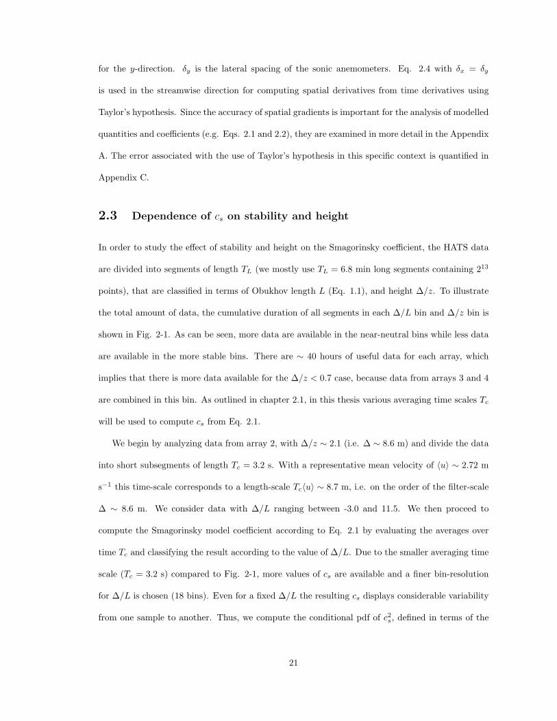
We begin by analyzing data from array 2, with ∆/z ∼ 2.1 (i.e. ∆ ∼ 8.6 m) and divide the data
into short subsegments of length Tc = 3.2 s. With a representative mean velocity of 〈u〉 ∼ 2.72 m
s−1 this time-scale corresponds to a length-scale Tc〈u〉 ∼ 8.7 m, i.e. on the order of the filter-scale
∆ ∼ 8.6 m. We consider data with ∆/L ranging between -3.0 and 11.5. We then proceed to
compute the Smagorinsky model coefficient according to Eq. 2.1 by evaluating the averages over
time Tc and classifying the result according to the value of ∆/L. Due to the smaller averaging time
scale (Tc = 3.2 s) compared to Fig. 2-1, more values of cs are available and a finer bin-resolution
for ∆/L is chosen (18 bins). Even for a fixed ∆/L the resulting cs displays considerable variability
from one sample to another. Thus, we compute the conditional pdf of c2s, defined in terms of the
21
Figure 2-1: Cumulative time of available data in each data bin. All 6.8 min data segments whoseaverage horizontal wind vector is less than 30o off the array-normal are binned according to their∆/L and ∆/z value. The height range (∆/z) is partitioned into 3 bins: array 1 (∆/z ∼ 4.3), array 2(∆/z ∼ 2.1) and arrays 3 and 4, which are combined (∆/z < 0.7). The stability range (∆/L) is par-titioned into 8 bins, whose end-points are given by the list [−2.0,−0.5, 0, 0.5, 1.0, 2.0, 4.0, 7.0, 10.0].
joint pdf P(c2s,∆/L
)according to
P
(c2s|
∆
L
)=
P(c2s,
∆L
)
P(
∆L
) , (2.5)
where P (∆/L) is the fraction of data contained in each ∆/L bin. In this fashion the dependence on
∆/L is isolated, independent of the amount of data in different stability bins in our data set (there
are much more near-neutral data than stably stratified data which biases the joint pdf P(c2s,∆/L
)
towards low values of ∆/L). To construct the pdf the range of c2s (−0.02 < c2
s < 0.04) is divided
into 120 bins. The resulting conditional pdf of the coefficient is shown using color contours in Fig.
2-2a for the c2s- and ∆/L-range where sufficient data are available. Repeating the procedure for a
longer averaging time Tc = 102.4 s, corresponding to about 32∆/〈u〉, we obtain the conditional pdf
shown in Fig. 2-2b.
22
Figure 2-2: Contour plots of conditional pdf of c2s, P
(c2s|∆/L
). The contours are spaced logarith-
mically. In (a) the averaging time to compute c2s is Tc = 3.2 s ∼ 1.0∆/〈u〉, whereas in (b) it is
Tc = 102.4 s ∼ 32∆/〈u〉. Results are from array 2 with ∆/z ∼ 2.1. The solid line is an empirical fitdescribed in Eq. 2.7. The dashed line shows c2
s = 0.
23
Fig. 2-2a shows that the most likely value of c2s depends strongly on stability. Specifically,
c2s decreases from values fluctuating around ∼ 0.015 in neutral conditions to smaller values for
increasing ∆/L. c2s is particularly sensitive to stability in the slightly stable region 0 < ∆/L < 0.5.
For unstable conditions, there is a large spread in c2s values around its conditional mean value,
whereas for very stable conditions all c2s fall within a narrower range. For unstable conditions
there is a significant amount of negative c2s. These events are called backscatter events, because
the resulting negative eddy viscosity causes an energy transfer from the SGS to the resolved scales
during the time period Tc. When the averaging time Tc for the computation of c2s is increased (Fig.
2-2b), the spread in c2s decreases significantly for near neutral conditions, while the pdf in stable
regions is almost unchanged. The most likely value for c2s is very similar to Fig. 2-2a. Moreover,
there are fewer events of negative c2s.
The mean and the variability of c2s around the most likely, or average, value and the statistics
of backscatter events will be addressed in more detail in chapter 2.5. Next, we include the effects
of distance to the ground (by considering results from different arrays).
Fig. 2-3 shows results for cs from averaging over segments of length Tc = TL = 13.7 min
∼ 283∆〈u〉 for the 4 different arrays. The data for arrays 3 and 4 are combined since they correspond
to similar values of ∆/z. As is visible, even after averaging over times corresponding to 283 filter
length-scales, there is significant variability. Nevertheless, it is seen that for all stabilities, the cs
values for large ∆/z tend to fall below those for low ∆/z, a trend that is consistent with previous
results (Mason 1994; Porte-Agel et al. 2000b, 2001b). No time segments of length Tc = 13.7 min
yielded a negative coefficient after averaging. In order to identify more clearly the trends with ∆/L
and ∆/z, averages are performed over the entire data available.
Fig. 2-4 shows results for cs from averaging SGS energy dissipations over all segments within
each ∆/L-bin of Fig. 2-1. Thus, these results correspond to using Tc equal to the times indicated in
Fig. 2-1 in each case. A very clear dependence of the coefficient on ∆/L and ∆/z can be identified.
Considering the heterogeneity of the data within one bin in respect to wind angle, turbulence
intensity, mean velocity, etc. it is reassuring that such clear trends emerge from the data. From its
24
−2 0 2 4 6 8 100
0.02
0.04
0.06
0.08
0.1
0.12
0.14
0.16
c s
∆/L
∆/z < 0.7∆/z ~ 2.1∆/z ~ 4.3
Figure 2-3: Smagorinsky coefficient cs as a function of ∆/L for an averaging time of Tc = 13.7 min ∼283∆〈u〉 for 3 different values of ∆/z. The symbols represent experimental results, the lines areempirical fits described in Eq. 2.7.
neutral value, cs decreases strongly under stable atmospheric conditions. Moreover, a larger ∆/z
leads to a decrease in the model coefficient, consistent with the use of damping functions for cs
close to the wall (see e.g. Mason and Thomson 1992), where z becomes equal to or smaller than ∆.
Based on the data in Fig. 2-4, a functional dependence of cs on both ∆/L and ∆/z is constructed.
To establish a functional dependence of cs on ∆/z, Eq. 1.15 for near-neutral stratification is written
as
cs = c0
[1 +
(c0
κ
∆
z
)n]−1/n
(2.6)
In addition, for stable stratification cs has to be decreased compared to its value in neutral condi-
tions. Considering the trends shown in Fig. 2-5a (which corresponds to Fig. 2-4 for ∆/L > 0 but
plotted in log-log coordinates to identify possible power-law scaling) we conclude that cs decreases
as cs ∼ (∆/L)−1 in very stable conditions for fixed ∆/z. In other words, the length-scale l = cs∆
scales as L in stably stratified conditions. This is consistent with results presented in Sullivan et al.
(2003) who show that l scales with the peak in the spectrum of vertical velocity. That length-scale
Figure 2-4: Smagorinsky coefficient cs as a function of ∆/L and ∆/z. Data segments of lengthTL = 6.8 min are classified according to their ∆/L values, for each of the 4 arrays. Eq. 2.1 is appliedto obtain cs using time averages of numerator and denominator over all segments. Depending onthe availability of data in each ∆/L-bin, the averaging time ranges from Tc = 0.8 hr to Tc = 22.9hr. The symbols represent these experimental results, the lines are empirical fits described in Eq.2.7. To test the fit for a different ∆/z value, cs is recomputed for a larger filter size ∆/z ∼ 8.6 usingdata from array 1 (downward facing triangles). Results obtained by Porte-Agel et al. (2001b) areincluded as open symbols.
is known to scale with L (Nieuwstadt 1984).
Thus a correction factor appropriate for the stable range is(1 + c0
α∆L
)−1, where α = O(c0) is a
model parameter. For large ∆/L this converges to (α/c0) (∆/L)−1
, whereas for small (but positive)
∆/L it approaches 1. Combining this expression with Eq. 2.6, and introducing the Ramp function
R(x) (R(x) = x if x > 0 and R(x) = 0 if x < 0) to avoid difficulties in the unstable range where
L < 0, we propose an expression of the form:
cs = c0
[1 +
c0
αR(
∆
L)
]−1 [1 +
(c0
κ
∆
z
)n]−1/n
. (2.7)
To further examine the validity of the proposed expression we consider the simultaneous limit of
large ∆/L and large ∆/z. For this limit (and n ≥ 1, say) Eq. 2.7 reduces to cs ∼ (∆/L)−1
(∆/z)−1
.
26
10−1
100
101
10−2
10−1
c s
∆/L
∆/z ~ 2.1c
s~(∆/L)−1
a)
10−2
10−1
100
101
102
10−2
10−1
c s
∆/L*∆/z
∆/z < 0.7∆/z ~ 2.1∆/z ~ 4.3c
s~∆−2
b)
Figure 2-5: (a) Same as Fig. 2-4 for ∆/L > 0 but plotted in log-log coordinates to identify possiblepower-law scaling. The dashed line shows a (∆/L)−1 scaling. (b) Smagorinsky coefficient cs as afunction of ∆/L × ∆/z for an averaging time of Tc = 13.7 min ∼ 283∆〈u〉. The symbols represent
experimental results, the dashed line shows a cs ∼(∆2
)−1scaling.
27
To test this asymptotic trend, in Fig. 2-5b cs is plotted vs. ∆/z × ∆/L for all arrays. Indeed, for
large ∆/L and large ∆/z cs follows closely the line cs ∼(∆2/ (Lz)
)−1justifying the proposed fit
in Eq. 2.7. This suggests that for ∆ ≫ L and ∆ ≫ z the value of cs is determined by the product
of the two length scales L and z rather than by the smaller of the two.
To fit the parameters of Eq. 2.7 to the data in Fig. 2-4 we set n = 3 and fit c0 and α using
multidimensional unconstrained nonlinear optimization from MATLAB. Mason and Brown (1999)
suggest n = 2, but the small differences between the cs of different arrays in neutral and unstable
conditions are indication of a slower decrease of cs with ∆/z, which requires a larger n. From the
optimization with n = 3, we obtain c0 = 0.1347, and α = 0.1289. Since the difference between c0
and α is within the range of experimental uncertainty, we assume α = c0 = 0.135. The resulting
equation is used for the fits in Fig. 2-4 as well as in the preceding Figs. 2-2 and 2-3.
The proposed fit is tested by comparison with a different set of data, namely from array 1 in
which a box filter is applied on 4 adjacent sonics in the “s”-array and the corresponding sonics
in the “d”-array. This results in a filter scale of ∆ = 26.8 m and a value of ∆/z = 8.6. Using a
one-sided derivative in the y-direction and a centered derivative in the x-direction, the quantities
needed to compute c2s from Eq. 2.1 are obtained and the results are shown in Fig. 2-4 as downward
facing triangles. We conclude that the proposed model fits these test-data quite well.
As a further test of the proposed fit, Fig. 2-6 compares the measured cs for an averaging time
Tc = TL = 13.7 min with the value obtained from Eq. 2.7. It can be concluded that the empirical fit
represents the mean trends in the data also for the shorter (compared to Fig. 2-4) averaging time.
However, for unstable conditions (large cs) deviations between the modelled and the measured cs
occur due to the large variability of the measured cs, whereas the model fit yields a constant value
of cs for any given value of ∆/z. Also, for arrays 3 and 4 (∆/z < 0.7) the scatter in the data is
larger than for arrays 1 and 2. This might be caused by the difference in setup geometry of array
3. There, the single filtered array is below the double filtered array (see table 2.1), which influences
and possibly overestimates vertical derivatives compared to the other setups. For array 4, different
filter types in the lateral direction are used for the single and double filtered arrays, as indicated in
Figure 2-6: Scatter plot of measured vs. modelled results for the Smagorinsky coefficient cs foran averaging time of Tc = 13.7 min. The symbols represent experimental results, the line markscmeass = cmod
s . The expression used to compute cmods is described in Eq. 2.7. Results obtained by
Porte-Agel et al. (2001b) are included as filled symbols.
table 2.1.
Analysis by other investigators has revealed similar results. Deardorff (1971) and Piomelli et al.
(1988) both found cs ≈ 0.1 for small ∆/z. Porte-Agel et al. (2001a) found cs ≈ 0.08 which is about
35% smaller than ours, but the tendency of an increase of the coefficient with ∆/z is the same.
The proposed expression in Eq. 2.7 can be easily used in LES, since ∆/L and ∆/z are known
parameters that are imposed in the simulations a priori by the choice of mesh-spacing, wall shear
stress and heat flux at the boundary. If the dependence on stratification is to be expressed as
a function of Richardson number, relationships between Ri and L/z can be used such as those
appearing in Businger et al. (1971). However, most of the recent work dealing with stability of the
lower atmosphere has tended to be in terms of L (Brutsaert 1982).
Finally, we report the coefficient values that are obtained from matching momentum flux instead
of dissipation, according to Eq. 2.3. Fig. 2-7 shows the coefficients so determined for various ∆/z
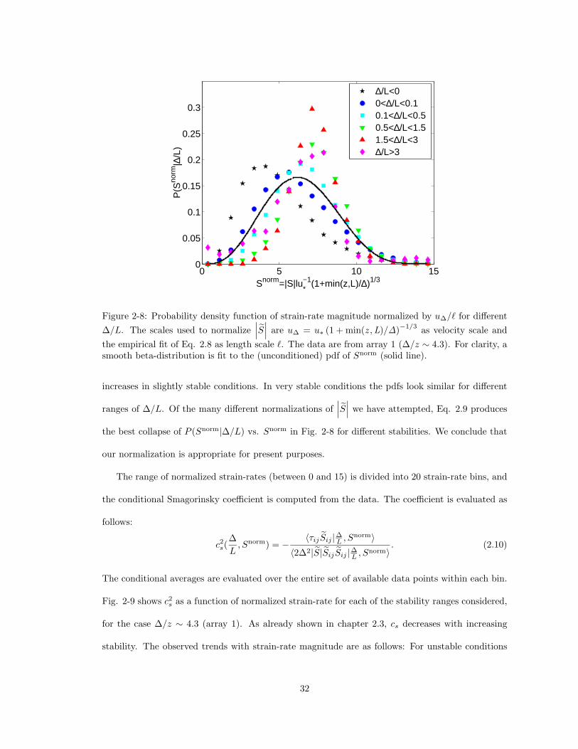
Figure 2-8: Probability density function of strain-rate magnitude normalized by u∆/ℓ for different
∆/L. The scales used to normalize∣∣∣S
∣∣∣ are u∆ = u∗ (1 + min(z ,L)/∆)−1/3
as velocity scale and
the empirical fit of Eq. 2.8 as length scale ℓ. The data are from array 1 (∆/z ∼ 4.3). For clarity, asmooth beta-distribution is fit to the (unconditioned) pdf of Snorm (solid line).
increases in slightly stable conditions. In very stable conditions the pdfs look similar for different
ranges of ∆/L. Of the many different normalizations of∣∣∣S
∣∣∣ we have attempted, Eq. 2.9 produces
the best collapse of P (Snorm|∆/L) vs. Snorm in Fig. 2-8 for different stabilities. We conclude that
our normalization is appropriate for present purposes.
The range of normalized strain-rates (between 0 and 15) is divided into 20 strain-rate bins, and
the conditional Smagorinsky coefficient is computed from the data. The coefficient is evaluated as
follows:
c2s(
∆
L, Snorm) = − 〈τijSij |∆L , Snorm〉
〈2∆2|S|SijSij |∆L , Snorm〉. (2.10)
The conditional averages are evaluated over the entire set of available data points within each bin.
Fig. 2-9 shows c2s as a function of normalized strain-rate for each of the stability ranges considered,
for the case ∆/z ∼ 4.3 (array 1). As already shown in chapter 2.3, cs decreases with increasing
stability. The observed trends with strain-rate magnitude are as follows: For unstable conditions
∣∣∣ ℓ/u∆ for different ∆/L. The scales used to normalize∣∣∣S
∣∣∣ are u∆ = u∗ (1 + min(z ,L)/∆)−1/3
as a velocity scale and the empirical fit of Eq. 2.8 as a length scale ℓ. The data are from array 1(∆/z ∼ 4.3).
(∆/L < 0) c2s decreases with strain-rate magnitude but only by a factor of about 2: values decrease
from c2s ∼ 0.02 at low Snorm to c2
s ∼ 0.01 at high Snorm. We remark that trends for Snorm < 2
are rather inconclusive and appear noisy, probably due to the small amount of data available in
these bins. In stable stratification (except for the case ∆/L > 3 which shows negligibly small
coefficients from which no trend with strain-rate can be discerned), the coefficient decreases quite
significantly with increasing local strain-rate magnitude. Typically the coefficient decreases about
five-fold between Snorm = 2 and Snorm = 10.
In order to isolate the effect of strain-rate magnitude, the conditional c2s values are normalized
by c2s(∆/L), the Smagorinsky coefficient conditioned on ∆/L for each array obtained by summing
over all strain-rate bins. Fig. 2-10 compares these normalized c2s for all three arrays, by considering
different stability ranges. Figure 2-10a is for unstable cases, 2-10b is for slightly stable cases, and
2-10c is for very stable cases. For large strain-rate magnitudes, a scaling of c2s ∼ (Snorm)
−1can
be identified for 1.5 < ∆/L < 3 in Fig. 2-10c. This slope becomes smaller in magnitude when
33
∆/L approaches zero (Fig. 2-10b) and c2s is found to be almost constant in unstable atmospheric
conditions (Fig. 2-10a). These trends are similar for all ∆/z-values (arrays). In terms of normalized
strain-rate magnitude, two regimes are identified. For large strain-rate magnitudes, c2s decreases
with Snorm. The other regime concerns small strain-rate magnitudes and shows an almost constant
Smagorinsky coefficient. The transition between these two regimes occurs at values of Snorm that
depend on ∆/L and ∆/z. The smaller ∆/L and the smaller ∆/z, the smaller the transition value
of Snorm. Fig. 2-10b exemplifies this statement. For ∆/z < 0.7 the transition region starts at
Snorm ∼ 4, for ∆/z ∼ 2.1 the value is Snorm ∼ 3 and for ∆/z ∼ 4.3 we find Snorm ∼ 2.
The implications for the Smagorinsky model are as follows. We conclude that the deeper ∆
is in the inertial range (∆ ≪ min(z ,L)) the more c2s is constant with Snorm implying that the
Smagorinsky scaling is valid. This becomes especially clear for the unstable to neutral data, for
which the weak dependence of c2s upon local strain-rate magnitude for all arrays provides support
for the basic scaling of the Smagorinsky model. However, the data for the stable cases show that
the Smagorinsky scaling is erroneous under conditions of stable stratification. As a consequence,
one may conclude that to properly scale the eddy-viscosity one must not only change the basic
length-scale (i.e. using ℓ as opposed to ∆) but also the velocity scale. More specifically, results
suggest that at large Snorm and ∆/L, the coefficient of Eq. 2.7 should be multiplied by a factor
[1 + β(∆/L)Snorm]−1
where β(∆/L) is some function that describes at what Snorm the transition
to a (Snorm)−1 scaling occurs. In the limit of large Snorm, the eddy viscosity would then scale
as c20ℓ
2(Snorm)−1∣∣∣S
∣∣∣ ∼ c20ℓu∆ with u∆ = u∗ (at large ∆/L), instead of c2
0ℓ2∣∣∣S
∣∣∣. The reasonable
collapse in our analysis suggests that the velocity scale u∆ may be more generally appropriate than
the conventional choice of ℓ∣∣∣S
∣∣∣. Finally, we recall that one has to differentiate between the scaling
with local strain-rate as it is examined here and the dependence on global shear as examined in
Hunt et al. (1988) and Canuto and Cheng (1997). In this thesis we consider the dependence on
global shear in the case of near-wall ABL to be already subsumed by the dependence upon ∆/z
that was considered in chapter 2.3.
34
100
101
10−1
100
101
Snorm=|S|lu*−1(1+min(z,L)/∆)1/3
c s2 (∆/
L,∆/
z,S
norm
) / c
s2 (∆/
L,∆/
z)∆/z~4.3∆/z~2.1∆/z~0.7
a)
∆/L<0
100
101
10−1
100
101
Snorm=|S|lu*−1(1+min(z,L)/∆)1/3
c s2 (∆/
L,∆/
z,S
norm
) / c
s2 (∆/
L,∆/
z)
∆/z~4.3∆/z~2.1∆/z~0.7
b)
0.1<∆/L<0.5
100
101
10−1
100
101
Snorm=|S|lu*−1(1+min(z,L)/∆)1/3
c s2 (∆/
L,∆/
z,S
norm
) / c
s2 (∆/
L,∆/
z)
∆/z~4.3∆/z~2.1∆/z~0.7
c)
1.5<∆/L<3
Figure 2-10: Log-log plots of Smagorinsky coefficient c2s conditioned on normalized strain-rate
magnitude Snorm for different stabilities ∆/L and arrays. (a) unstable: ∆/L < 0, (b) slightlystable: 0.1 < ∆/L < 0.5, (c) very stable: 1.5 < ∆/L < 3. In (b,c) the dashed line has a slope of -1,and shows an inverse power-law behavior.
35
2.5 Variability of cs
In this section we address the question ”how variable is cs?”. Results shown in chapter 2.3, specif-
ically Figs. 2-2a and b, suggest that while the most likely value of c2s does not change significantly
with averaging time Tc, the variability of the coefficient decreases for increasing Tc, at least for
the near-neutral and unstable cases. To quantify the dependence of the statistics of cs on Tc and
stability, pdfs of cs are computed for different values of ∆/L and Tc. Two stability bins are se-
lected for the analysis. The first bin contains unstable atmospheric conditions characterized by
−2.0 < ∆/L < 0.0. The second bin groups data under very stable conditions. Since there are less
overall data available for large ∆/L, in order to obtain reasonably well-converged pdfs, we choose
a wide bin of stabilities, namely 1.5 < ∆/L < 5.5. Five different values of Tc are selected, ranging
from Tc = 3.2 s to Tc = 205 s. Fig. 2-11a shows the resulting pdfs for the unstable data, while the
very stable data are presented in Fig. 2-11b. Backscatter events are excluded from the analysis to
focus on cs > 0. The probability P (c2s < 0) is less than 0.2 (as will be shown later in Fig. 2-13).
Fig. 2-11a shows that the spread in the pdf of cs increases for decreasing Tc for unstable
atmospheric stability. Reassuringly, however, the most likely value of cs and the median (as shown
in Fig. 2-12a) do not depend on Tc. For stable conditions (Fig. 2-11b), the most likely value
and the median (Fig. 2-12a) of cs are constant with Tc and smaller than for unstable conditions,
in agreement with the findings in chapter 2.3. The fact that the medians of cs are independent
of Tc for stable and unstable conditions is encouraging for LES with dynamic SGS models which,
as discussed in the introduction, often use some kind of averaging procedures, either in space (e.g.
horizontal planes) or time (e.g. the Lagrangian dynamic model (Meneveau et al. 1996)) to compute
the coefficient. Our results suggest that correct median coefficients can be obtained even for fairly
short averaging time-scales. Rather surprisingly, however, in the case of stable conditions it appears
that the spread in the pdf does not decrease for increasing Tc.
Fig. 2-12b presents a quantification of the width of the pdfs as a function of Tc. Instead of
computing the rms value (which tends to be biased due to some outliers in the distribution), we
36
0 0.05 0.1 0.15 0.2 0.25
10−1
100
101
cs
P(c
s)
Tc= 3.2s
Tc= 6.4s
Tc=12.8s
Tc=51.2s
Tc= 205s
a)
0 0.01 0.02 0.03 0.04 0.05 0.06
10−1
100
101
cs
P(c
s)
Tc= 3.2s
Tc= 6.4s
Tc=12.8s
Tc=51.2s
Tc= 205s
b)
Figure 2-11: Pdf of Smagorinsky coefficient cs for different averaging times Tc (see legend) for (a)unstable atmospheric stability conditions (−2.0 < ∆/L < 0.0) and (b) very stable atmosphericstability conditions (1.5 < ∆/L < 5.5). The advection time through one filter scale is roughly∆/〈u〉 = 5.4 s. The data are from array 1 (∆/z ∼ 4.3).
37
quantify the spread of the pdfs with quartiles. The figure shows the difference between the third
and first quartile of the distribution, normalized by the second quartile (thus giving a dimensionless
measure of the variability that is not strongly affected by atypical outliers). The relative width of
the pdf for the stable bin does not decrease as Tc is increased. This result shows strong variability
of the real and/or modelled SGS dissipation (in the numerator and denominator of Eq. 2.1) under
stable atmospheric conditions indicating that fluctuations occur over very long time-scales. This
may be related to the strong intermittency in stable atmospheric conditions.
The fraction of segments of length Tc that display average backscatter (with negative c2s over
the time Tc) that were neglected in the preceding analysis of chapter 2.5 is shown in Fig. 2-13 as a
function of Tc. As expected, the fraction diminishes with increasing Tc because backscatter events
tend to be cancelled by forward-scatter events within the time-interval Tc, yielding a positive c2s on
average. Consistent with Sullivan et al. (2003) we find that the fraction of time with backscatter
events increases with z/∆ (not shown). Sullivan et al. (2003) report a ratio of backscattered energy
to total transferred energy of 0.2 for this array configuration.
2.6 Results for coefficients in scalar models
As introduced in Eq. 2.2, the coefficient for the Smagorinsky model for the SGS heat flux Pr−1T c2
s
can be computed by matching SGS dissipations of scalar variance. Similar to Fig. 2-2b, in Fig.
2-14a the conditional pdf of Pr−1T c2
s is presented. The data are from array 2 with averaging time
Tc = 102.4 s. Similar to Fig. 2-2b, the coefficient decreases under stable conditions, and shows
more variability in unstable conditions.
By dividing c2s by Pr−1
T c2s for each data segment, the Prandtl number is obtained and plotted
in Fig. 2-14b. Most values of PrT lie between 0 and 1 independent of stability. For unstable to
neutral conditions the most likely value of PrT increases from PrT ∼ 0.3 to PrT ∼ 0.8, and over the
stable range a clear tendency is not apparent. The spread in the conditional pdf does not change
significantly with stability. In the following the dependencies of Pr−1T c2
s and PrT are examined in
38
10−1
100
101
102
0
0.02
0.04
0.06
0.08
0.1
0.12
Tc [s]
q2 (cs)
unstablevery stable
a)
10−1
100
101
102
0.1
0.2
0.3
0.4
0.5
0.6
0.7
0.8
0.9
1
Tc [s]
(q3 (c
s)−q1 (c
s))/q
2 (cs)
unstablevery stable
b)
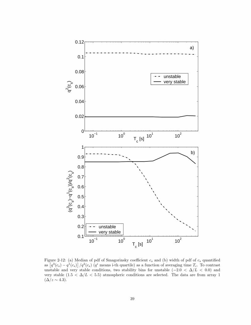
Figure 2-12: (a) Median of pdf of Smagorinsky coefficient cs and (b) width of pdf of cs quantifiedas
[q3(cs) − q1(cs)
]/q2(cs) (qi means i-th quartile) as a function of averaging time Tc. To contrast
unstable and very stable conditions, two stability bins for unstable (−2.0 < ∆/L < 0.0) andvery stable (1.5 < ∆/L < 5.5) atmospheric conditions are selected. The data are from array 1(∆/z ∼ 4.3).
39
10−1
100
101
102
0
0.02
0.04
0.06
0.08
0.1
0.12
0.14
0.16
0.18
Tc [s]
frac
tion
of ti
me
with
bac
ksca
tter
unstablevery stable
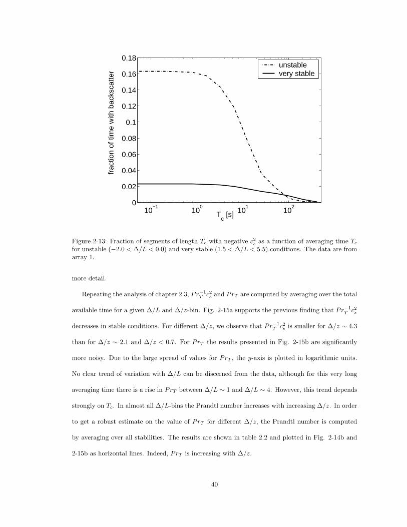
Figure 2-13: Fraction of segments of length Tc with negative c2s as a function of averaging time Tc
for unstable (−2.0 < ∆/L < 0.0) and very stable (1.5 < ∆/L < 5.5) conditions. The data are fromarray 1.
more detail.
Repeating the analysis of chapter 2.3, Pr−1T c2
s and PrT are computed by averaging over the total
available time for a given ∆/L and ∆/z-bin. Fig. 2-15a supports the previous finding that Pr−1T c2
s
decreases in stable conditions. For different ∆/z, we observe that Pr−1T c2
s is smaller for ∆/z ∼ 4.3
than for ∆/z ∼ 2.1 and ∆/z < 0.7. For PrT the results presented in Fig. 2-15b are significantly
more noisy. Due to the large spread of values for PrT , the y-axis is plotted in logarithmic units.
No clear trend of variation with ∆/L can be discerned from the data, although for this very long
averaging time there is a rise in PrT between ∆/L ∼ 1 and ∆/L ∼ 4. However, this trend depends
strongly on Tc. In almost all ∆/L-bins the Prandtl number increases with increasing ∆/z. In order
to get a robust estimate on the value of PrT for different ∆/z, the Prandtl number is computed
by averaging over all stabilities. The results are shown in table 2.2 and plotted in Fig. 2-14b and
2-15b as horizontal lines. Indeed, PrT is increasing with ∆/z.
40
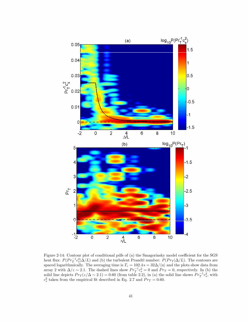
Figure 2-14: Contour plot of conditional pdfs of (a) the Smagorinsky model coefficient for the SGSheat flux: P (Pr−1
T c2s|∆/L) and (b) the turbulent Prandtl number: P (PrT |∆/L). The contours are
spaced logarithmically. The averaging time is Tc = 102.4 s = 32∆/〈u〉 and the plots show data fromarray 2 with ∆/z ∼ 2.1. The dashed lines show Pr−1
T c2s = 0 and PrT = 0, respectively. In (b) the
solid line depicts PrT (z/∆ ∼ 2.1) = 0.60 (from table 2.2), in (a) the solid line shows Pr−1T c2
s, withc2s taken from the empirical fit described in Eq. 2.7 and PrT = 0.60.
Figure 2-15: Smagorinsky model coefficients (a) Pr−1T c2
s and (b) PrT as a function of ∆/L fordifferent ∆/z. Note that the y-axis in (b) is in logarithmic units. TL = 6.8 min data segmentsare classified according to their ∆/L values, for each of the 4 arrays. For each ∆/L value, Eq. 2.2is applied to obtain Pr−1
T c2s using time averages of numerator and denominator over all segments.
PrT is computed by dividing c2s computed from Eq. 2.1 by Pr−1
T c2s. Depending on the availability
of data in each ∆/L-bin, the averaging time ranges from Tc = 0.8 hr to Tc = 22.9 hr. The lines areempirical fits. The fits are constructed from Eq. 2.7 (for c2
s) and from table 2.2 for PrT . Resultsobtained by Porte-Agel et al. (2001b) are included as open symbols.
42
∆/z ∼ 4.3 ∆/z ∼ 2.1 ∆/z < 0.7
PrT 0.67 0.60 0.49
Table 2.2: Prandtl number PrT conditioned on ∆/z computed from Eqs. 2.1 and 2.2 assumingthat PrT is not a function of stability. The averaging time is the total time available for each array(Tc > 35 hours).
In order to quantify the variability of PrT , the analysis of chapter 2.5 is repeated. All data
segments with −2.0 < ∆/L < 0.0 (unstable bin) and 1.5 < ∆/L > 5.5 (stable bin) are selected
and PrT (∆/L) is computed with varying averaging times Tc. Then the quartiles of the resulting
probability distribution of PrT are obtained and the median q2 is plotted in Fig. 2-16a. In contrast
to our findings concerning cs, the median of the Prandtl number is not constant, but increases
with Tc. This explains the difference between Fig. 2-15b and 2-14b, in which PrT computed from
averages over several hours in Fig. 2-15b was significantly larger than PrT computed from 102.4 s
averages in Fig. 2-14b. The increase with averaging time appears to level off for Tc > 102 s. For
all Tc, the median for very stable conditions is larger than the median for unstable conditions, but
they seem to converge for large Tc. A similar behavior (but with different magnitudes of Prandtl
numbers) is observed for the other arrays. The dependence of the median of PrT on the averaging
time and the large scatter in Fig. 2-14b complicate the development of empirical expressions for
PrT and Pr−1T c2
s. Thus we only present definitive results on the dependence of PrT upon ∆/z (as
shown in table 2.2), and refrain from attempting to fit the ∆/L dependence.
In comparing with prior results, we can remark that for small ∆/z, Mason and Derbyshire
(1990), Moin et al. (1991), and Porte-Agel et al. (2001a) found PrT ∼ 0.4, which is within the
range of uncertainty around our value of PrT (∆/z < 0.7) = 0.49. For large ∆/z, Porte-Agel et al.
(2001a) examined two 30 min segments whose ∆/z roughly correspond to the values for our arrays
1 and 2. For the setup similar to our array 2 they obtain PrT ∼ 0.5 for ∆/L = −0.26, their analysis
of the setup similar to our array 1 results in PrT ∼ 0.6 for ∆/L = −1.18. Our results from table
2.2 suggest PrT = 0.60 and PrT = 0.67, which is qualitatively consistent and within the range of
43
10−1
100
101
102
0
0.2
0.4
0.6
0.8
1
Tc [s]
q2 (Pr T
)
unstablevery stable
a)
10−1
100
101
102
0
0.2
0.4
0.6
0.8
1
1.2
1.4
1.6
1.8
Tc [s]
(q3 (P
r T)−
q1 (Pr T
))/q
2 (Pr T
)
unstablevery stable
b)
Figure 2-16: (a) Median of pdf of Prandtl number q2(PrT ) and (b) width of pdf of PrT quantifiedas
[q3(PrT ) − q1(PrT )
]/q2(PrT ) (qi means i-th quartile) as a function of averaging time Tc. To
contrast unstable and very stable conditions, two stability bins for unstable (−2.0 < ∆/L < 0.0)and very stable (1.5 < ∆/L < 5.5) atmospheric conditions are selected. The data are from array 1(∆/z ∼ 4.3).
44
experimental uncertainty.
The spread of the pdf of PrT is shown in Fig. 2-16b as a function of Tc. For unstable atmospheric
stability conditions, (q3−q1)/q2 decreases from a value of 1.7 to 0.3 for Tc ranging from Tc = 0.05 s
to 6.8 min. For very stable conditions the variability is constant between 0.3 and 0.6 for the entire
range of Tc. This is in agreement to findings for the variability of cs in chapter 2.5. Possibly due to
the intermittency in stable conditions the variability does not decrease for larger averaging times,
while in unstable conditions the variability decreases significantly. The results for arrays 1, 3 and
4 are very similar.
2.7 Conclusions
Parameters of the Smagorinsky model for the SGS shear stress and the SGS heat flux have been
studied based on a statistical analysis of a large data set (157 hours) of ABL turbulence. Model
coefficients have been measured based on the condition of equivalence between real and modelled
SGS dissipation of kinetic energy and scalar variance. Several trends have been identified. Consis-
tent with prior results in the literature, near the ground it is found that cs depends on the ratio
of filter length and height above the ground, ∆/z, and decreases as ∆/z is increased. Moreover,
cs depends strongly on atmospheric stability as parameterized by the length-scale ratio ∆/L. The
previously postulated decrease of cs in stable stratification and shear (Deardorff 1980; Canuto and
Cheng 1997) is quantified from the data and an empirical formula (Eq. 2.7) for cs is proposed.
By varying the time Tc over which the SGS energy dissipations are averaged, we find that the
variability in cs decreases with increasing Tc for unstable to neutral conditions, whereas in very
stable conditions the variability in cs is independent of averaging time. The fact that in either case
the median of cs is independent of averaging time confirms the robustness of the results. It also
supports the assumption inherent in the Lagrangian dynamic SGS models that coefficients can be
obtained from data by averaging over time-scales that are not overly long.
The dependence of cs on local strain-rate magnitude has also been studied here. Since the
45
Smagorinsky model already assumes proportionality of the eddy viscosity νT to strain-rate magni-
tude∣∣∣S
∣∣∣, cs should be independent of strain-rate magnitude. The data suggest that this is correct
for unstable to neutral conditions or for small strain-rate magnitudes. However, in stable condi-
tions and for large strain-rate magnitudes, cs decreases with strain-rate magnitude. In very stable
conditions the data are consistent with a c2s ∼
∣∣∣S∣∣∣−1
scaling. The transition value of the strain-rate
magnitude between these two regimes is found to depend on stability and ∆/z. This result shows
that the usual velocity scale, ℓ∣∣∣S
∣∣∣, is inappropriate under stable conditions, even when correcting
the length-scale from ∆ to L (i.e. using ℓ). Instead, the friction velocity provides a better scale
for prescribing the eddy-viscosity when the turbulence is limited by stable stratification, but one
still has to account for the fact that the velocity scale has to be smaller than u∗ when ∆ is in the
inertial range.
A similar analysis is carried out for the coefficient of the SGS heat flux Pr−1T c2
s and the derived
turbulent Prandtl number PrT . The strong decrease of Pr−1T c2
s in stable conditions comes mostly
from the strong dependence of c2s on stability, while we observe that PrT depends only weakly on
stability. A robust increase of PrT with increasing ∆/z, going from PrT ∼ 0.49 for ∆/z < 0.7,
to PrT ∼ 0.67 for ∆/z ∼ 4.3, is observed. The observed dependence of the median of PrT on
the averaging time Tc and general variability of the results precludes us from stating unambiguous
conclusions on the dependence of PrT on stability. Results for the SGS heat flux models show more
scatter than those for the SGS stress models, most likely because of larger experimental uncertainty
in the temperature gradients than in the velocity gradients. In general, the coefficient of the SGS
heat flux model Pr−1T c2
s behaves very similarly to c2s. Thus for the remainder of this thesis we
concentrate on the coefficient in the momentum equations.
Finally the basic flaws of the eddy viscosity models need to be pointed out. Even perfect knowl-
edge of the coefficient does not result in correct prediction of both energy transfer from the resolved
scales to the subgrid-scales and the momentum fluxes associated with the SGS stress. Moreover, the
basic proportionality assumption of the Smagorinsky model τij ∝ ∆2|S|Sij is contradicted by ten-
sorial misalignment between SGS stress and strain-rate (Tao et al. 2002), independent of the value
46
of cs. Even with these limitations, the eddy-viscosity closure is still the most-often used in practical
applications, providing continued interest in the dependence of cs on physical flow parameters as
studied here.
47
Chapter 3
Predictions from dynamic SGS models and
comparisons with measured Smagorinsky
coefficients
3.1 Dynamic SGS models
In the simplest SGS model the SGS stress defined in Eq. 1.9 can be expressed in terms of velocity
gradients by the Smagorinsky model (Eq. 1.12, Smagorinsky 1963). Once the basic eddy-viscosity
closure is accepted, the most crucial remaining parameter to choose is the Smagorinsky coefficient
c(∆)s . In traditional LES of atmospheric boundary layers, c
(∆)s is deduced from phenomenological
theories of turbulence (Lilly 1967, Mason 1994).
Along a fundamentally different line of thinking, Germano et al. (1991) proposed the “dynamic
model”. Instead of prescribing a priori a model for c(∆)s as a function of flow parameters, this
approach is based upon the idea of analyzing the statistics of the simulated large-scale field (during
LES) to determine the unknown model coefficient. The dynamic model is based on the Germano
identity (Germano 1992),
Lij ≡ uiuj − uiuj = Tα∆ij − τ∆
ij . (3.1)
48
Above, Lij is the resolved stress tensor and T α∆ij = uiuj − uiuj is the stress at a test-filter scale
α∆ (an overline (..) denotes test filtering at a scale α∆). In simulations, α is typically chosen to
be α = 2. If one applies this dynamic procedure by replacing T α∆ij and τ∆
ij by their prediction from
the basic Smagorinsky model the result is:
Lij −1
3δijLkk =
(c(∆)s
)2
Mij , where Mij = 2∆2
∣∣∣S∣∣∣ Sij −
(αc
(α∆)s
)2
(c(∆)s
)2
∣∣∣S∣∣∣ Sij
. (3.2)
To proceed, the crucial assumption in the standard dynamic model (Germano et al. 1991) is
scale invariance of the coefficient, namely
c(∆)s = c(α∆)
s . (3.3)
This step allows the only remaining unknown parameter in Eq. 3.2, c(∆)s , to be obtained. The
overdetermined system of equations can be solved by minimizing the square error averaged over
all independent tensor components (Lilly 1992), and some spatial domain (Ghosal et al. 1995) or
temporal domain (Meneveau et al. 1996). The result is:
(c(∆)s
)2
=〈LijMij〉〈MijMij〉
. (3.4)
Here the symbol 〈..〉 denotes ensemble, time or spatial averaging, depending on the context. The
dynamic model has been successfully applied to a variety of engineering flows (see Meneveau &
Katz 2000 and Piomelli 1999 for reviews). In general, it provides realistic predictions of c(∆)s when
the flow field is sufficiently resolved, i.e. the test-filter scale α∆ is smaller than the local integral
scale of turbulence.
In the context of ABL turbulence the dynamic Smagorinsky model has been implemented in an
LES by Porte-Agel et al. (2000b). They examined the scale-invariance hypothesis and the dynamic
49
model with LES of a neutral ABL. They found that near the wall streamwise energy spectra decay
too slowly, indicating that the dynamically determined coefficient is too small. In addition, by
running four simulations at different resolutions they demonstrated a clear scale-dependence of
the Smagorinsky coefficient (c(∆)s 6= c
(α∆)s ), which violates the scale-invariance assumption of the
dynamic model (Eq. 3.3). As a consequence Porte-Agel et al. (2000b) proposed a scale-dependent
dynamic model. In addition to a test-filter at α∆, a test-filter at α2∆ (denoted by a hat below)
delivers another equation similar to Eq. 3.2:
Qij −1
3δijQkk =
(c(∆)s
)2
Nij , where Qij = uiuj − uiuj (3.5)
Nij = 2∆2
∣∣∣S∣∣∣ Sij −
(α2c
(α2∆)s
)2
(c(∆)s
)2
∣∣∣∣S
∣∣∣∣Sij
. (3.6)
With this additional equation the scale-invariance assumption can be relaxed. A new parameter,
β, is defined according to
β =
(c(α∆)s
)2
(c(∆)s
)2 . (3.7)
Under the assumption that β is constant independent of ∆, which is equivalent to assuming a
power-law behavior c(∆)s ∼ ∆Φ, the two equations 3.2 and 3.6 can be solved for the two unknowns
c(∆)s and β (Porte-Agel et al. 2000b). The solution procedure for β is detailed in Appendix B.
Porte-Agel et al. (2000b) applied the scale-dependent dynamic SGS model to an LES of a neutral
boundary layer and obtained realistic results for mean velocity gradients and streamwise energy
spectra.
The objective of the present study is to examine field data at various length scales and determine
whether the dynamic model yields realistic predictions of the coefficient c(∆)s and its dependencies
upon distance to the ground and atmospheric stability. Both the scale-invariant (Germano et al.
1991) and the more elaborate scale-dependent form (Porte-Agel et al. 2000b) of the dynamic model
will be examined. The current chapter uses the field data presented in chapter 2.2 but processed at
a different set of length scales to perform the various filtering operations required for the dynamic
50
models. We also investigate how the averaging time scale influences the results. As indicated in
Eq. 3.4 the dynamic model requires averaging of data. Knowledge of an appropriate averaging
time scale is relevant for the Lagrangian SGS model (Meneveau et al. 1996) which determines the
model coefficient by accumulating weighted averages over fluid path lines. However, due to the
experimental conditions, only Eulerian averaging can be used in this study.
The present chapter is organized as follows: In chapter 3.2, we describe the field experiment and
the data processing techniques. Chapter 3.2 also contains a brief review of the results in chapter
2.3: measured distributions of c(∆)s as a function of height and stratification. In chapter 3.3 the
ability of the scale-invariant dynamic and scale-dependent dynamic SGS models to reproduce the
behavior of c(∆)s is studied. Conclusions are presented in chapter 3.4.
3.2 Data set and processing
3.2.1 The HATS data set for dynamic models
The HATS experiment was described in detail in chapter 2.2 and Horst et al. (2004). In chapter
2.3, the dependence of c(∆)s on different relevant length scales was examined: height above ground,
z, filter scale ∆, and the Obukhov length L (Eq. 1.1).
Out of a total of four field setups with different geometrical arrangements, only two had sensor
arrangements so that they can be used to dynamically determine Smagorinsky coefficients. These
setups are presented in Table 3.1.
Figure 3-1 shows a schematic of the instrument setup for arrays 1 and 2. To compute SGS
quantities, the velocity fields have to be spatially filtered in two dimensions at a scale ∆. Since
the velocities will also be filtered at two larger scales, α∆ and α2∆, ∆ is chosen to be smaller
than the values used in chapter 2. Here we use ∆ = 2δy where δy is the lateral spacing of the
sonic anemometers. Discrete versions of a trapezoidal filter function are applied in the lateral (y)
direction and a smoother Gaussian filter is used in the streamwise (x) direction. For details see
chapter 2.2.
51
Array Data zd − d0 zs − d0 δy ∆ ∆zd−d0
〈ud〉
# [h] [m] [m] [m] [m] [-] [m s−1]
1 46.0 3.13 6.58 3.35 6.70 2.1 2.46
2 38.7 4.01 8.34 2.17 4.34 1.1 2.72
Table 3.1: Array properties for the HATS experiment. “d”: double filtered array, “s”: single filteredarray, d0: displacement height, δy: lateral instrument spacing, ∆: filter size.
Gradients are calculated with finite differences (FD). In the vertical direction (x3 = z), the
setup necessitates a first order one-sided FD ∂u/∂z|zd= (zs − zd)
−1 [u(zs) − u(zd)]. In the hori-
zontal directions, a 2nd-order centered FD scheme is used, e.g. for the y-direction: ∂ui/∂y|y0=
(2δy)−1
[ui(y0 + δy) − ui(y0 − δy)]. Assuming Taylor’s hypothesis, the same formula with δx = δy
is used in the streamwise direction to compute ∂ui/∂x.
In order to depict the available data as a function of stability and array, in chapter 2 the data
was divided into segments of length 6.8 min. These segments were classified according to stability,
parameterized as Obukhov length L non-dimensionalized by the filter size ∆. The distribution of
data by stability can be seen in Fig. 2-1, for various heights (parameterized as ∆/z). In the present
chapter we use the same procedure and data classification. In the following, the procedures to
compute the model coefficient as a function of the parameters will be described in more detail.
3.2.2 Empirically determined Smagorinsky coefficient: procedures and
results
The “real” value of c(∆)s for LES is determined from the field data by matching mean measured
and modeled SGS dissipations Π∆ (Eq. 2.1). In this case we use our time series of some particular
length, a time scale Tc. In chapter 2.3 we analyzed the behavior of c(∆,emp)s from HATS data as a
function of parameters ∆/z and ∆/L. A fit to the data for cs as a function of ∆/L and ∆/z was
proposed in Eq. 2.7.
52
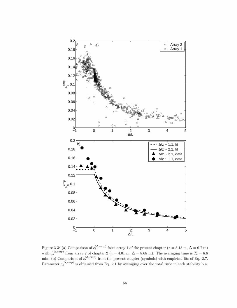
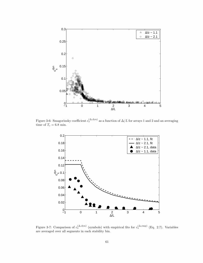
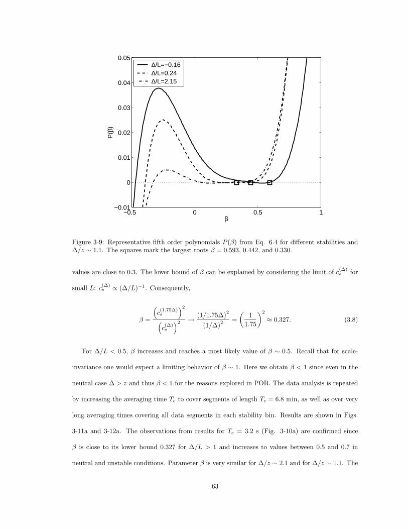
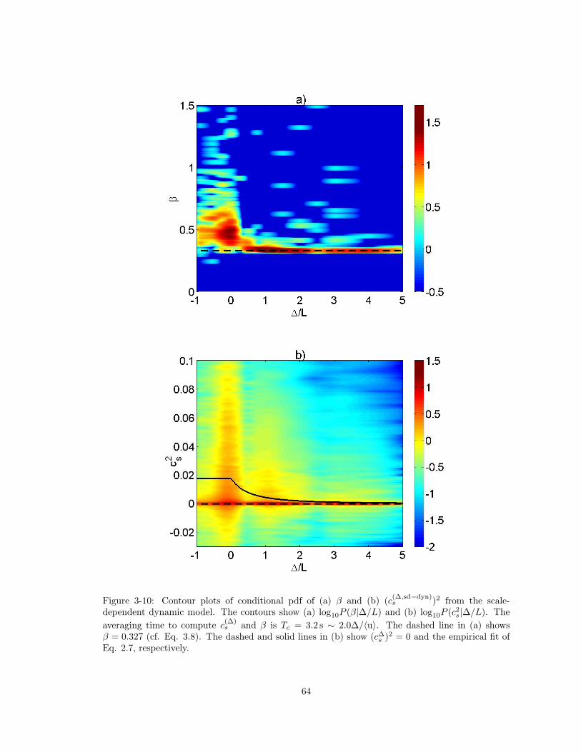
Figure 3-1: Experimental setup of HATS. 3D sonic anemometers are displayed as circles. Thereference number of the instrument is to the upper left and the measured or computed variable atthis location is to the right. (a) unfiltered variables. Sample lateral filter weights for a scale ∆ aremarked in grey below locations 1 - 2, and 9 - 11. (b) variables filtered at scale ∆. Sample lateralfilter weights are displayed below locations 7, 9 and 11, which are hatched. (c) variables filtered atscale 1.75∆.
In the present chapter, the filter size is only half of that in chapter 2. Figure 3-1a provides a
sketch of the filtering procedures in the transverse (y or x2) direction. A three-point trapezoidal
filter with weights [0.25, 0.5, 0.25] is used in the lower array and a two-point filter with weights
[0.5, 0.5] is used in the upper array. In the streamwise direction, the Gaussian filter is used as
described in the preceding section. Thus filtered velocities ui, and SGS stresses τij , at a scale
∆ = 2δy are available at locations 7 - 13 and between locations 1 - 5 (Fig. 3-1b). As a result, the
filtered strain rate tensors can be obtained at locations 9 and 11, using 2nd order centered FD in the
horizontal and 1st order one-sided FD in the vertical directions, respectively. Since τij is available
at these locations as well, the Smagorinsky coefficients c(∆,emp)s are evaluated at locations 9 and 11.
The results from these two locations are essentially identical and only results from location 9 are
presented.
53
A first question to address is whether the data analyzed at scale ∆ = 2δy provide results that are
consistent with those of chapter 2 that were obtained at a larger scale, using more sensors from each
array. To compare the current results with chapter 2, data from array 2 (∆/z ∼ 1.1) is divided into
stability bins from ∆/L = −1 to ∆/L = 5 and further divided into subsegments of length Tc = 3.2
s. This corresponds roughly to a length scale Tc〈u〉 ∼ 8.7 m which is on the order of twice the filter
scale ∆ ∼ 4.3 m. The empirically determined Smagorinsky model coefficient c(∆,emp)s is obtained
by evaluating the averages in Eq. 2.1 over time Tc. In order to isolate the dependence on ∆/L,
we compute the conditional pdf of (c∆,emps )2, P
(c2s|∆L
)= P
(c2s,
∆L
)/P
(∆L
), where P (∆/L) is the
fraction of data contained in each ∆/L bin. The (c∆s )2 range (−0.03 < (c∆
s )2 < 0.1) is divided
into 260 bins. Figure 3-2 shows the conditional pdf of (c∆,emps )2 using color contours. The figure
confirms the results of chapter 2: c(∆,emp)s decreases in stable conditions and its pdf shows a large
spread in unstable conditions with a considerable number of negative values. The most likely value
of c(∆,emp)s corresponds well to the empirical fit of chapter 2. Liu et al. (1995) obtained the eddy
viscosity field without averaging and also found a highly variable eddy viscosity field with negative
values, which causes numerical instabilities in LES.
The comparison with chapter 2 is repeated using a larger averaging time scale Tc. Fig. 3-3a
shows a direct comparison of data from array 1 (∆/z ∼ 2.1) of the present chapter with data from a
better resolved filter but same ∆/z from array 2 of chapter 2 for an averaging time scale of Tc = 6.8
min. The results agree very well, even though they are obtained from two different arrays. The
agreement confirms that the curves collapse for a given ∆/z, independent of the dimensional values
of ∆ or z. Finally, in Fig. 3-3b we perform a comparison based on the global time averages of
SGS dissipations. Here we average the terms in Eq. 2.1 over all data available in each ∆/L bin,
obtaining a single measured value of c(∆,emp)s in each bin. The coefficients are very close to the lines
which are the predictions from the fit of chapter 2. Only in unstable conditions are the predictions
about ∼ 10% too small. Besides confirming the collapse of the data, this comparison shows that
despite the coarse filter resolution in the lateral direction (using only two or three sensors) the
resulting measured coefficients agree with the results of using finer lateral resolutions.
54
Figure 3-2: Contour plots of conditional pdf of (c∆,emps )2, P
(c2s|∆/L
), for array 2 (∆/z ∼ 1.1). The
contours show log10P (c2s|∆/L). The averaging time to compute c
(∆)s is Tc = 3.2 s ∼ 2.0∆/〈u〉. The
solid line is the empirical fit of Eq. 2.7. The dashed line shows (c∆s )2 = 0.
To provide a systematic description of the effects of averaging time Tc upon the statistics of
c(∆,emp)s , the main aspects of the pdf of c
(∆,emp)s are documented as a function of Tc. Fig. 3-4
displays the median of c(∆,emp)s as a function of Tc for different stabilities. As reported in chapter
2, the median of c(∆,emp)s is constant with averaging time and much smaller in stable conditions
than in unstable and neutral conditions. In unstable conditions the median increases slightly with
averaging time. A measure of the spread of the pdf is documented in terms of the difference between
third and first quartile normalized by the second quartile. As expected, this measure decreases with
increasing Tc, in neutral and unstable conditions. As reported in chapter 2, the decrease is weaker
in stable conditions, which can be attributed to larger intermittency in stable conditions.
Figure 3-3: (a) Comparison of c(∆,emp)s from array 1 of the present chapter (z = 3.13 m, ∆ = 6.7 m)
with c(∆,emp)s from array 2 of chapter 2 (z = 4.01 m, ∆ = 8.68 m). The averaging time is Tc = 6.8
min. (b) Comparison of c(∆,emp)s from the present chapter (symbols) with empirical fits of Eq. 2.7.
Parameter c(∆,emp)s is obtained from Eq. 2.1 by averaging over the total time in each stability bin.
56
10−3
10−2
10−1
100
101
102
103
10−3
10−2
10−1
100
101
102
Tc [s]
med
ian(
c s2 ),[q
3 (cs2 )−
q1 (cs2 )]
/q2 (c
s2 )
q2 unstable(q3−q1)/q2 un.q2 neutral(q3−q1)/q2 n.q2 stable(q3−q1)/q2 st.
Figure 3-4: Median q2 and spread(q3 − q1
)/q2 of the (c∆,emp
s )2 distribution as a function ofaveraging time scale Tc for different stabilities: unstable (−0.5 < ∆/L < −0.25), near neutral(0 < ∆/L < 0.25), and stable (2 < ∆/L < 2.5). The data are from array 2.
3.2.3 Scale-invariant dynamic Model: procedures
In order to obtain the dynamic model coefficient from Eq. 3.4, filtered strain-rate tensors and
velocity vectors at a scale ∆ have to be filtered at α∆ to evaluate Lij and Mij . Usually α = 2, but
the limited maximum filter width in the lateral direction requires us to use α = 1.75 in the present
study. As shown in Germano et al. (1991), the sensitivity of the dynamic coefficient to α is not
expected to be important. Figure 3-1b shows that Sij at a scale ∆ can be obtained at locations 7, 9,
11, and 13. At locations 9 and 11 Sij is computed from centered horizontal FD and one-sided vertical
FD. At locations 7 and 13, the horizontal and the vertical FD are one-sided. A filter of size 1.75∆ is
applied on ui, Sij ,∣∣∣S
∣∣∣, and∣∣∣S
∣∣∣ Sij . The filter weight wi associated with a variable (already filtered
at scale ∆) at location yi, used to compute a test-filtered variable at location yα∆ is evaluated as
follows: w∗i = |[yi − ∆/2, yi + ∆/2] ∩ [yα∆ − α∆/2, yα∆ + α∆/2]|, where [yi − ∆/2, yi + ∆/2] is
the segment of length ∆ surrounding the point yi, and [yα∆ − α∆/2, yα∆ + α∆/2] is the segment of
57
length α∆ surrounding the point yα∆. Variables yi and yα∆ are the y coordinates of the instrument
at location i and the test-filtered variable, respectively. Weights w∗i are normalized so that they sum
up to 1: wi = w∗i /
∑i w∗
i . This procedure gives weights of wi = [0.214, 0.571, 0.214] for locations
i=[7, 9, 11] and i=[9, 11, 13]. Using the test-filtered variables, the time series of LijMij and MijMij
are computed at locations 9 and 11, averaged over a time scale Tc, and divided to obtain c(∆,dyn)s
using Eq. 3.4.
3.2.4 Scale-dependent dynamic Model: procedures
The scale-dependent dynamic coefficient is obtained similarly to procedures described in section
3.2.3. The filtered strain rate tensors and filtered velocity vectors of Fig. 3-1b are now, however,
filtered at α2∆ = 1.752∆. The same weighting scheme as in chapter 3.2.3 produces weights of
wi = [0.18, 0.32, 0.32, 0.18] for strain-rate tensors at locations [7, 9, 11, 13]. The resulting∣∣∣S
∣∣∣ Sij ,
and
∣∣∣∣S
∣∣∣∣Sij are used to compute Nij , while uiuj , and ui are used to compute Qij .
It is important to note that Nij is a function of β. Parameter β is computed using procedures
identical to those in Porte-Agel et al. (2000b, hereafter POR). Six coefficients of a fifth order
polynomial in β are obtained from averaging products of strain rates and resolved stresses over Tc,
as described in Appendix B (Eqs. 6.4-6.12). Then the roots of the polynomial in β are determined
by the “roots” function in MATLAB (The Mathworks Inc.). As argued in POR, only the largest
real root is physically meaningful. A time series of Qij and Nij is obtained from Eq. 3.6 using
the β value which was derived from quantities averaged over Tc. Finally, the scale-dependent
dynamic procedure yields the coefficient at a scale ∆ as (c(∆,sd−dyn)s )2 = 〈QijNij〉/〈NijNij〉 or
(c(∆,sd−dyn)s )2 = 〈LijMij〉/〈MijMij〉.
58
3.3 Smagorinsky coefficients determined from dynamic SGS models
3.3.1 Scale-invariant dynamic model: results
To begin, the scale-invariant, dynamically determined Smagorinsky model coefficient c(∆,dyn)s is
obtained according to chapter 3.2.3 by evaluating the averages over time Tc = 3.2 s for array 2.
Figure 3-5 shows the pdf of (c(∆,dyn)s )2 conditioned on ∆/L using color contours. It is apparent
that the most likely value of (c(∆,dyn)s )2 depends on stability. It is very close to zero for ∆/L > 1
and increases strongly in near neutral conditions (∆/L ∼ 0). In neutral and unstable conditions,
the spread in the pdf is large with a considerable number of negative values. These trends are
consistent with those of the empirical coefficient reported in chapter 3.2.2. However, comparing
the color contours with the line from the fit in Eq. 2.7 and with the conditional pdf of c(∆,emp)s in
Fig. 3-2, it can be seen that the dynamically determined coefficients are too small, especially in
conditions of stable stratification (∆/L > 0).
Figure 3-6 shows the empirically and dynamically determined coefficient for a longer averaging
time Tc = 6.8 min and for arrays 1 and 2. At this averaging scale too, the results confirm that
the dynamic model predicts a coefficient which is significantly smaller than c(∆,emp)s . Finally, the
same results are obtained when performing the averages over all available data as shown in Fig.
3-7, where one value of c(∆,dyn)s is plotted for each ∆/L-bin.
The dynamic procedure predicts the correct basic trends of the coefficient with stability (∆/L)
and height (∆/z), but the magnitudes of the coefficients are too small by significant factors. In
unstable and neutral conditions, factors range from 2-5. In very stable conditions this factor is as
large as an order of magnitude or more. Thus the energy transfer (Π∆) from resolved scales to SGS
is too small, and in LES using such a model one would expect a high-wavenumber pile-up of energy
in the spectra near the wall. This weakness of the dynamic model was already observed in LES
of the ABL in neutral conditions (POR), and present results suggest that this weakness would be
acerbated in conditions of stable stratification.
The variability of c(∆,dyn)s is examined in Fig. 3-8 by plotting the quartiles of the (c∆,dyn
s )2
59
Figure 3-5: Contour plots of the pdf of (c∆,dyns )2 conditioned on ∆/L for array 2 (∆/z ∼ 1.1). The
contours show log10P (c2s|∆/L). The averaging time to compute c
(∆)s is Tc = 3.2 s ∼ 2.0∆/〈u〉. The
solid line is the empirical fit of Eq. 2.7. The dashed line shows (c∆s )2 = 0.
distribution for different averaging times Tc. The median of c(∆,dyn)s is very similar for Tc ranging
from 0.05 s (no averaging) to hours. The relative spread of the pdf decreases with averaging time
which agrees with results from chapter 2 and Fig. 3-4 for c(∆,emp)s .
In summary, the results for c(∆,dyn)s consistently show that the dynamic procedure under-predicts
the Smagorinsky coefficient when ∆ is close to, or exceeds L, or z, or both. This deficiency is not
surprising. As suggested by the very same empirical fit through the available data for c(∆,emp)s
(Eq. 2.7), for any fixed value of z or L the coefficient is dependent upon ∆ unless ∆ << L and
∆ << z. Thus, the expected behavior of the coefficient contradicts the basic assumption of scale-
invariance underlying the dynamic model. This was already noted in POR for the neutral case but
∆ > z. The scale-dependent dynamic model described in chapter 3.2.4 addresses this problem. In
the following section we analyze the data to study whether the scale-dependent model yields more
realistic predictions of the coefficient compared to the standard dynamic model.
60
−1 0 1 2 3 4 50
0.05
0.1
0.15
0.2
0.25
0.3
∆/L
c sdyn
∆/z ~ 1.1∆/z ~ 2.1
Figure 3-6: Smagorinsky coefficient c(∆,dyn)s as a function of ∆/L for arrays 1 and 2 and an averaging
Figure 3-7: Comparison of c(∆,dyn)s (symbols) with empirical fits for c
(∆,emp)s (Eq. 2.7). Variables
are averaged over all segments in each stability bin.
61
10−3
10−2
10−1
100
101
102
103
10−5
10−4
10−3
10−2
10−1
100
101
Tc [s]
med
ian(
c s2 ),[q
3 (cs2 )−
q1 (cs2 )]
/q2 (c
s2 )
q2 unstable(q3−q1)/q2 un.q2 neutral(q3−q1)/q2 n.q2 stable(q3−q1)/q2 st.
Figure 3-8: Median q2 and spread(q3 − q1
)/q2 of the (c∆,dyn
s )2 distribution as a function ofaveraging time scale Tc for different stabilities: unstable (−0.5 < ∆/L < −0.25), near neutral(0 < ∆/L < 0.25), and stable (2 < ∆/L < 2.5). The data are from array 2.
3.3.2 Scale-dependent dynamic model: results
Analysis for the scale-dependent dynamic model first requires computation of the parameter de-
scribing scale-dependence of the Smagorinsky coefficient, β = (cα∆s )2/(c∆
s )2. Again, data from array
2 (∆/z ∼ 1.1) are divided into bins of different stabilities ranging from ∆/L = −1 to ∆/L = 5,
and divided into subsegments of length Tc. Parameter β is obtained according to chapter 3.2.4.
Specifically, we use Eqs. 6.4-6.12. Averages such as⟨∣∣∣S
∣∣∣ SijLij
⟩or
⟨∣∣∣∣S
∣∣∣∣2 Sij
Sij
⟩are evaluated
over a time scale Tc. Figure 3-9 shows a few representative polynomials P (β) for the case Tc = 6.8
min, for three values of ∆/L. The largest root is the value of β that solves the condition of Eq. 6.3
and 6.4 (POR).
Parameter β is computed for the short duration averaging time of Tc = 3.2, and β is obtained in
each segment. The conditional pdf of β is presented in Fig. 3-10a, where the β range (0 < β < 1.5)
is divided into 150 bins. Note that β also depends on stability. In very stable conditions most β
62
−0.5 0 0.5 1−0.01
0
0.01
0.02
0.03
0.04
0.05
β
P(β
)
∆/L=−0.16∆/L=0.24∆/L=2.15
Figure 3-9: Representative fifth order polynomials P (β) from Eq. 6.4 for different stabilities and∆/z ∼ 1.1. The squares mark the largest roots β = 0.593, 0.442, and 0.330.
values are close to 0.3. The lower bound of β can be explained by considering the limit of c(∆)s for
small L: c(∆)s ∝ (∆/L)−1. Consequently,
β =
(c(1.75∆)s
)2
(c(∆)s
)2 → (1/1.75∆)2
(1/∆)2 =
(1
1.75
)2
≈ 0.327. (3.8)
For ∆/L < 0.5, β increases and reaches a most likely value of β ∼ 0.5. Recall that for scale-
invariance one would expect a limiting behavior of β ∼ 1. Here we obtain β < 1 since even in the
neutral case ∆ > z and thus β < 1 for the reasons explored in POR. The data analysis is repeated
by increasing the averaging time Tc to cover segments of length Tc = 6.8 min, as well as over very
long averaging times covering all data segments in each stability bin. Results are shown in Figs.
3-11a and 3-12a. The observations from results for Tc = 3.2 s (Fig. 3-10a) are confirmed since
β is close to its lower bound 0.327 for ∆/L > 1 and increases to values between 0.5 and 0.7 in
neutral and unstable conditions. Parameter β is very similar for ∆/z ∼ 2.1 and for ∆/z ∼ 1.1. The
63
Figure 3-10: Contour plots of conditional pdf of (a) β and (b) (c(∆,sd−dyn)s )2 from the scale-
dependent dynamic model. The contours show (a) log10P (β|∆/L) and (b) log10P (c2s|∆/L). The
averaging time to compute c(∆)s and β is Tc = 3.2 s ∼ 2.0∆/〈u〉. The dashed line in (a) shows
β = 0.327 (cf. Eq. 3.8). The dashed and solid lines in (b) show (c∆s )2 = 0 and the empirical fit of
Eq. 2.7, respectively.
64
magnitude of β in the present analysis compares well with Fig. 10 in POR. They obtain a significant
increase from β ∼ 0.5 at ∆/z = 2 to β ∼ 0.65 at ∆/z = 1.1 in neutral conditions (∆/L = 0), quite
consistent with present field measurement results. The limit of large z/∆ (∆ << z), where the
turbulence is better resolved, cannot be verified with the HATS data for which ∆ is comparable
or larger than z. Figure 3-13 shows that the median of β is constant with averaging time and the
variability decreases with Tc.
The model coefficient, c(∆,sd−dyn)s , predicted from the scale-dependent dynamic model, is ob-
tained by replacing the measured β value in the expression for Nij (see chapter 3.2.4). The analysis
is performed again using several averaging times Tc = 3.2 sec, Tc = 6.8 min, as well as a large Tc
encompassing all available data in each bin. As before, results for Tc = 3.2 s are presented in terms
of a conditional pdf for c(∆,sd−dyn)s , for the case ∆/z ∼ 1.1, and −1 < ∆/L < 5 in Fig. 3-10b. The
general trend in the relationship with stability is similar to that observed for c(∆,dyn)s in Fig. 3-5,
but the spread in the pdf is considerably larger. The most likely value of the coefficient seems to
be larger (and hence more accurate) than the scale-invariant dynamic model coefficient. However,
the large variability in c(∆,sd−dyn)s prevents us from stating this as a definitive conclusion at this
short averaging time scale.
Results from the intermediate time scale Tc = 6.8 min, in which β computed at that time scale
is used, are shown in Fig. 3-11b. Results clearly show that the scale dependent dynamic model
predicts c(∆,emp)s quite well in unstable and neutral conditions. In stable conditions, the prediction
is still improved compared to the dynamic model (Fig. 3-6), but significant scatter persists. Finally,
we present results using the longest Tc, by averaging over the entire data set in each stability bin.
Results are shown in Fig. 3-12b. As can be seen c(∆,sd−dyn)s obtained from long-time averaging
predicts c(∆,emp)s and its dependence on stability and height quite accurately.
The variability of c(∆,sd−dyn)s is examined in Fig. 3-13b. The variability is larger than for c
(∆,emp)s
and c(∆,dyn)s and for all stability bins more than 25% of the recorded (c∆,sd−dyn
s )2 are negative. The
variability reduces subsequently for Tc > 3.2 s. Also, in unstable conditions the median increases
significantly with averaging time for Tc > 3.2 s. If a reasonable criterion is introduced which
65
−1 0 1 2 3 4 50
0.5
1
1.5
∆/L
β
∆/z ~ 1.1∆/z ~ 2.1
a)
−1 0 1 2 3 4 50
0.05
0.1
0.15
0.2
0.25
0.3
∆/L
c ssd−
dyn
∆/z ~ 1.1∆/z ~ 2.1
b)
Figure 3-11: (a) β and (b) c(∆,sd−dyn)s as a function of ∆/L for arrays 1 and 2. The averaging time
is Tc = 6.8 min.
66
−1 0 1 2 3 4 50
0.1
0.2
0.3
0.4
0.5
0.6
0.7
0.8
0.9
1
∆/L
β
∆/z ~ 1.1∆/z ~ 2.1
a)
−1 0 1 2 3 4 50
0.02
0.04
0.06
0.08
0.1
0.12
0.14
0.16
0.18
0.2
∆/L
c ssd−
dyn
∆/z~1.1,fit∆/z~2.1,fit∆/z~2.1,data∆/z~1.1,data
b)
Figure 3-12: (a) Scale-dependence parameter β for array 1 (∆/z ∼ 2.1) and array 2 (∆/z ∼ 1.1).
(b) Comparison of c(∆,sd−dyn)s (symbols) with empirical fits for c
(∆,emp)s (Eq. 2.7). Variables are
averaged over all segments in each stability bin.
67
10−3
10−2
10−1
100
101
102
103
10−2
10−1
100
Tc [s]
med
ian(
β),[q
3 (β)−
q1 (β)]
/q2 (β
)
q2 unstable(q3−q1)/q2 un.q2 neutral(q3−q1)/q2 n.q2 stable(q3−q1)/q2 st.
10−3
10−2
10−1
100
101
102
103
10−3
10−2
10−1
100
101
102
Tc [s]
med
ian(
c s2 ),[q
3 (cs2 )−
q1 (cs2 )]
/q2 (c
s2 )
q2 unstable(q3−q1)/q2 un.q2 neutral(q3−q1)/q2 n.q2 stable(q3−q1)/q2 st.
Figure 3-13: Median q2 and spread(q3 − q1
)/q2 of the (a) β and (b) (c∆,sd−dyn
s )2 distributions asa function of averaging time scale Tc for different stabilities: unstable (−0.5 < ∆/L < −0.25), nearneutral (0 < ∆/L < 0.25), and stable (2 < ∆/L < 2.5). The data are from array 2.
68
requires the median of c(∆,sd−dyn)s to differ less than 10% from the median of c
(∆,emp)s , then Fig.
3-13b suggests that the Eulerian averaging time scale Tc should correspond to at least 12.8 s, or
about eight filter scales (8 ≈ 12.8〈u〉/∆).
To confirm that we have obtained results that are unique to turbulence signals under the present
physical conditions and do not occur for any time series of random numbers, the procedure to
compute dynamic and scale-dependent dynamic coefficients is tested with a time series of random
velocity vectors. We generate random velocity fluctuations by distributing 3d vectors whose length
is sampled from a uniform distribution in [0, 1] m s−1, and whose direction is uniformly distributed
over a sphere. Both white-noise and colored-noise signals (with a -5/3 energy spectrum for each
velocity component) are used. The resulting c(∆,emp)s , c
(∆,dyn)s , c
(∆,sd−dyn)s feature symmetric pdfs
with a strong peak at (c(∆)s )2 = 0, i.e. as expected random signals do not have the correlations
between Lij and Mij associated with net energy flux to smaller scales and a non-zero value of the
coefficient. The resulting pdf for β is positively skewed, increasing for β > 0.327 and but reaching
a peak at β ∼ 0.45. This is significantly different from the results of the present chapter, where e.g.
the peak in P (β|∆/L) for stable conditions in Fig. 3-10a is narrow and much closer to 0.327.
3.4 Conclusions
Predictions of the scale-invariant dynamic SGS model (Germano et al. 1991) and the scale-
dependent dynamic SGS model (Porte-Agel et al. 2000b) for the Smagorinsky coefficient c(∆)s
have been tested a priori with a large data set from two horizontal arrays of fourteen 3D-sonic
anemometers in the atmospheric surface layer. Figures 3-14a and 3-14b summarize the results by
comparing the empirically determined c(∆,emp)s with predictions from scale-invariant dynamic and
scale-dependent dynamic models, for both values of ∆/z considered. Clearly, the scale-invariance
assumption of the dynamic model breaks down when the filter size is large (∆ > z or ∆ > L),
resulting in coefficients that are too small. In LES of the ABL this is expected to lead to unrealistic
velocity profiles near the surface and a pile-up of energy reflected in flat velocity spectra.
69
−1 0 1 2 3 4 50
0.02
0.04
0.06
0.08
0.1
0.12
0.14
0.16
0.18
0.2
∆/L
c s
empdynsd−dyn
a)
−1 0 1 2 3 4 50
0.02
0.04
0.06
0.08
0.1
0.12
0.14
0.16
0.18
0.2
∆/L
c s
empdynsd−dyn
b)
Figure 3-14: Smagorinsky coefficient c(∆)s as a function of ∆/L for different SGS models. Variables
are averaged over all segments in each stability bin. (a) array 1, ∆/z ∼ 2.1 (b) array 2, ∆/z ∼ 1.1.
70
The scale-dependent dynamic model accounts for scale-dependence of the coefficient. As a
result the predicted coefficient is close to the real measured value. Note that despite the success of
the scale-dependent dynamic model in predicting the coefficient which produces the correct SGS
dissipation, it is reiterated that even “perfect” prediction of the coefficient does not necessarily
result in correct prediction of the SGS stress tensor, for reasons discussed in the introduction.
The data suggest that the Eulerian averaging time scale of the scale-dependent dynamic model
should be at least ∼ 8 times the time scale associated with the filter scale. Such a time scale is
somewhat larger than averaging time scales usually employed in the Lagrangian dynamic model
(Meneveau et al 1996). However, due to the fundamental differences between Lagrangian and
Eulerian averaging the applicability of the result to Lagrangian averaging is uncertain and remains
to be explored in simulations.
71
Chapter 4
Dynamic subgrid-scale models in Large Eddy
Simulation
4.1 Introduction
A Large Eddy Simulation (LES) with dynamic SGS models is performed in order to study the ac-
curacy of the predicted mean flow velocities, and compare the predictions of cs with those measured
in the field. Specifically, the prediction of the coefficient from the dynamic procedure introduced
in chapter 3.2 applied in LES is compared to a priori tests from the HATS experiment.
In that way the applicability of a priori results in field experiments to a posteriori settings in
LES can be studied. As in chapter 3, both the scale-invariant and scale-dependent dynamic models
will be examined. The main difference between the experimental analysis and the simulations is
the type of averaging employed to measure the coefficients: In the a priori analysis of chapter 3,
Eulerian time averaging over times Tc was performed. In the simulations, we use time averaging
along fluid pathlines (Lagrangian averaging). Lagrangian averaging is required for the general
applicability of dynamic models to flows in complex geometries which do not possess directions of
statistical homogeneity.
In chapters 2 and 3, stability parameter ∆/L accurately characterized the experimental data
from the lowest 10 m in the ABL. The Obukhov length L is a surface layer length scale and the
72
surface layer (z < 10 m at night, z < 100 m during the day) quickly responds to changes in surface
boundary conditions (heat flux and friction velocity). This assumption is confirmed by the good
collapse of measurements of cs with ∆/L in the HATS experiment. The LES domain, however,
extends beyond the surface layer and spans the entire height of the ABL (∼ 2 km). There, ∆/L
is not expected to be an appropriate length scale. The Richardson number, on the other hand, is
expected to be a parameter that may be applicable throughout the ABL. Hence, before showing
the simulations and results, we begin by recasting the HATS measured results in terms of the
Richardson number, in addition to the Obukhov length L used before.
4.2 HATS results in terms of Richardson number
The Richardson number is a stability parameter measuring the ratio of buoyant to mechanical
production of turbulent kinetic energy. Flux and gradient Richardson numbers are defined as
Rif =〈w′θ′〉 g
〈θ〉
〈u′w′〉∂〈u〉∂z + 〈v′w′〉∂〈v〉
∂z
, (4.1)
Rig =
∂〈θ〉∂z
g〈θ〉(
∂〈u〉∂z
)2
+(
∂〈v〉∂z
)2 , (4.2)
respectively. Dynamic stability criteria state that laminar flows become turbulent for Rig < 0.25
and turbulent flows become laminar for Rig > 1.0 (Stull 1997). Unstable flows are characterized
by Rif < 0 and Rig < 0. In LES, the Richardson number has often been used to parameterize cs
as a function of stability in simulations. For instance, Lilly (1962) parameterizes the eddy viscosity
as νT = λ2r
∣∣∣S∣∣∣ (1 − Ripf ) where λr is a characteristic subgrid length scale and Ripf is the pointwise
flux Richardson number (without the averaging operation of Eq. 4.1). Lilly (1962) proposed this
model with λr = λ, where λ is the “basic mixing length”, i.e. the height-dependent mixing length
in neutral conditions. This approach only considers the direct influence of buoyancy on the energy
production and it was intended for unstable conditions only. In our notation Lilly’s model implies
that λ = cs(∆/z,Ripf = 0)∆ and thus cs(∆/z,Ripf ) = c0
[1 +
(c0
κ∆z
)n]−1/n
(1 − Ripf )0.5. Brown
73
et al. (1994, hereafter BDM) also account for the influence of buoyancy on the length scales by
making λr dependent on Ripg.
νT = λ2∣∣∣S
∣∣∣ fm(Ripg) (4.3)
From field experimental data in the surface layer, they propose a functional dependence of the
length scale on stability by expressing the function fm in Eq. 4.3 as
fm = (1 − 16Ripg)0.5 for Ripg < 0 (4.4)
fm =(1 − Ripg/Ricg
)4for 0 < Ripg < Ricg (4.5)
fm = 0 for Ripg > Ricg. (4.6)
Since λ2fm(Ripg) = c2s(∆/z,Ripg)∆
2, we can write BDM’s model as
cs(∆/z,Ripg) = c0
[1 +
(c0
κ
∆
z
)n]−1/n [fm(Ripg)
]0.5. (4.7)
To compare with this model, the HATS data is plotted against Rig in (Fig. 4-1). HATS data
from array 1 (upper plots) and array 2 (lower plots) for two different filter size ∆ = 2δ and ∆ = 4δ
are presented and compared to the proposed model by BDM and the fit of chapter 2 (Eq. 2.7).
For this purpose, empirical relationships by Businger et al. (1971) have been used to express L as
a function of Rig:
Rig = z/L when L < 0 (4.8)
Rig =z
L
0.74 + 4.7z/L
(1 + 4.7z/L)2 when L > 0. (4.9)
Since Eq. 2.7 has been fit to the very same data, the good agreement between data and fit in Fig.
4-1 only supports the validity of the empirical conversion relationships (Eqs. 4.8 and 4.9). In Fig.
4-1 it can be observed, that when Rig is larger than the critical Richardson number (Ricg ∼ 0.25),
c2s is close to 0. For 0 < Rig < Ricg, c2
s increases dramatically. The model of Eq. 2.7 (which has
74
−1 −0.5 0 0.50
0.05
0.1
0.15
c s
∆/z=2.0701
HATSBrown 94Kleissl 03R
c=0.25
−1 −0.5 0 0.50
0.05
0.1
0.15
∆/z=1.0415
Rig
−1 −0.5 0 0.50
0.05
0.1
0.15c s
∆/z=4.1403
−1 −0.5 0 0.50
0.05
0.1
0.15
Rig
∆/z=2.0829
c s
Figure 4-1: Results from the HATS experiment as a function of gradient Richardson number.Proposed expressions for cs by Brown et al. (1994) and Kleissl et al. (2003) are also shown.
been fit to the very same data) agrees very well with the data in stable conditions (Rig > 0). Thus
it can be used to represent the HATS data in comparisons with results from LES in chapters that
follow. BDM’s model also fits the data well, but underpredicts c2s for ∆/z ∼ 1. Clearly, BDM
strongly overpredict c2s under unstable conditions (Rig < 0).
The rest of this chapter is organized as follows: The LES code is described in chapter 4.3. In
chapter 4.4 the Lagrangian dynamic model and different procedures for averaging the numerators
and denominators needed to calculate the dynamic coefficient in the simulation are presented. Two
test cases in stable and unstable conditions are analyzed in chapter 4.5. A simulation with a heat
flux and geostrophic wind forcing corresponding to a diurnal cycle is presented in chapter 4.6.
75
Predictions for cs from the simulation are compared to HATS results in chapter 4.7. Conclusions
follow in chapter 4.8.
4.3 Numerical simulations
The boundary conditions for the simulation are selected to resemble as much as possible the mea-
sured conditions during HATS on September 6, 2000. This day is selected because it includes typical
features that are representative to the entire data set. Various meteorological variables measured
in the field are presented in Fig. 4-2 as a time series of 5 minute averages. A typical diurnal heat
flux variation is observed with a maximum 〈w′θ′〉s of 0.3 K m s−1 and a minimum of 0.03 K m
s−1. As can be seen, wind speeds at a height z = 3.45 m are significantly lower at nighttime than
at daytime. The weak winds lead to low friction velocity u∗, which in turn creates a very stably
stratified boundary layer (e.g. ∆/L up to 10).
A 64 x 64 x 64 grid staggered in the vertical, and spanning a domain of 6283 m x 6283 m x
2000 m is simulated. The filtered Navier-Stokes equations are integrated over time based on the
numerical approach described in Albertson and Parlange (1999, 2000).
Variable θ′ = θ − 〈θ〉 describes temperature fluctuations and qj is the SGS heat flux
qi = −Pr−1T c2
s∆2∣∣∣S
∣∣∣ ∂θ
∂xi, (4.13)
where PrT is the turbulent SGS Prandtl number, which is set to PrT = 0.4. The Coriolis parameter
f = sin Φ × 1.45 × 10⁻⁴s−1 is imposed, using Φ ∼ 36o N for the latitude of the HATS array. The
velocity field is forced by a geostrophic wind velocity (ug, vg) (Eq. 4.12).
76
18 24 6 1218027036090
180
win
d di
rect
ion
time [h]
18 24 6 120
3
6
(u2 +
v2 )1/2
18 24 6 12−1000
0
1000
L [m
]
18 24 6 12
0
5
10
∆/L
18 24 6 120
0.3
0.6
u * [m s
−1 ]
18 24 6 120
0.10.20.3
<w
′ tc′
> [K
m s
−1 ]
Figure 4-2: Observed meteorological conditions on 9/6/2000 in Kettlemen City, CA. The mea-surement height is z = 3.45 m. The time is PST (Pacific Standard Time). The wind directionperpendicular to the array is marked by a solid line, deviations of ±30o are marked by dashed lines.
77
The horizontal boundary conditions are periodic and the vertical boundary conditions are zero
vertical velocity and imposed stress at the bottom and no-stress at the top. The surface shear
stresses are prescribed using the Monin-Obukhov similarity law:
τ13 = −(
κ
ln z/zo − ψm
)2 (u
2+ v
2)0.5
u (4.14)
τ23 = −(
κ
ln z/zo − ψm
)2 (u
2+ v
2)0.5
v, (4.15)
where () represents a local average from filtering the velocity field at 2∆. The roughness length
at the surface is set to zo = 0.02 m, equivalent to the value determined from the HATS data,
and κ = 0.4. The flux-profile functions in unstable conditions are given by Dyer (1974) with the
correction by Hogstrom (1987). In stable conditions we use the formulation by Cheng and Brutsaert
(2004, personal communication):
φm = (1 − 15.2z/L)−1/4 when L < 0 (4.16)
φm = 1 + 6.1z/L + (z/L)2.5
(1 + (z/L)2.5
)−1+1/2.5
z/L + (1 + (z/L)2.5)1/2.5
when L > 0 (4.17)
The ψm functions are determined as
ψm(z/L) =
∫ z/L
zo/L
[1 − φm(x)] dx/x (4.18)
A sponge at the four levels below the top is applied to dissipate energy of gravity waves before
they reach the upper boundary of the domain (Nieuwstadt et al. 1993). Pseudospectral treatment
is used in horizontal planes and second-order finite finite differencing is implemented in the verti-
cal direction. The second order accurate Adam-Bashforth scheme is used for time-advancement.
Nonlinear convective terms and the SGS stress are dealiased using the 3/2 rule (Orszag 1970). The
simulations are forced with prescribed geostrophic velocity (ug, vg) and surface heat flux 〈w′θ′〉s.
Figure 4-3 shows the initial mean temperature and mean velocity profile of the simulations. A
78
300 305 3100
200
400
600
800
1000
1200
1400
1600
1800
2000
θ [K]
z [m
]
6 7 8 90
200
400
600
800
1000
1200
1400
1600
1800
2000
u [m s−1]
Figure 4-3: Initial mean temperature and mean velocity profile of the simulation.
stably stratified layer with a large temperature gradient 〈∂θ/∂z〉 = 0.012 K m−1 is created at the
top to limit the growth of the boundary layer in daytime. The boundary layer height zi is used as
a characteristic length scale.
4.4 The Lagrangian dynamic SGS model
First we consider the scale-invariant model with cα∆s = c∆
s . As reviewed in chapter 1.3, the
Smagorinsky coefficient c2s in LES needs to be averaged over homogeneous areas or over time in
order to prevent negative eddy viscosities that lead to numerical instabilities. Typically in channel
flow, or ABL flow, c2s is computed from quantities averaged over horizontal planes. However, over
heterogeneous surfaces, spatial averaging over large planes is not appropriate, whereas time aver-
aging in a Lagrangian sense can be physically motivated (Meneveau et al. 1996). The Lagrangian
dynamic model is based on Germano’s identity (Eq. 3.1) which upon replacing the stresses with
79
the Smagorinsky model expression yields
Lij =(c(∆)s
)2
Mij . (4.19)
To determine the ideal value of cs (cs has to match five independent tensor components), Lilly
(1992) defines an error function
ǫ = Lij −(c(∆)s
)2
Mij . (4.20)
In the traditional formulation, the square error is minimized by averaging over horizontal planes
(Eq. 3.4). Here, the coefficient c(∆)s is obtained by minimizing the weighted time average of the
where x(t′) are the positions of the fluid elements at time t′, and W (t) is a weighting function. The
minimum of E occurs when
(c(∆)s
)2
=ILM
IMM, (4.22)
where ILM and IMM are defined as
ILM =
∫ t
−∞
LijMij (x(t′), t′)W (t − t′)dt′ (4.23)
IMM =
∫ t
−∞
MijMij (x(t′), t′)W (t − t′)dt′. (4.24)
When the weighting function W (t) is chosen to be an exponentially decreasing function, IMM and
ILM are the solutions to two relaxation transport equations which can be easily implemented in
LES. These transport equations read:
∂ILM
∂t+ u · ∇ILM =
1
T(LijMij − ILM ) (4.25)
80
∂IMM
∂t+ u · ∇IMM =
1
T(MijMij − IMM ) (4.26)
The model uses W (t − t′) = T−1 exp [(t − t′)/T ], where the time scale T is chosen based on
several criteria (see Meneveau et al. 1996) according to
T = 1.5∆ (ILMIMM )−1/8
. (4.27)
Among others, this choice ensures that in regions where LijMij is negative (and would produce
negative coefficients without averaging), the time-scale increases inhibiting the average ILM from
ever becoming negative. For further details see Bou-Zeid et al. (2004) and Meneveau et al. (1996).
4.4.1 Inclusion of scale-dependence in the Lagrangian dynamic SGS model
The Lagrangian SGS model described above relies on scale-invariance of the Smagorinsky coefficient.
This was proven to be an incorrect assumption in conditions of small turbulence integral scales (see
chapter 3 and POR). A dynamic scale-dependent version of the Lagrangian SGS model is currently
under development (Bou-Zeid et al. 2004 - personal communication), but not yet operational at
the time of writing of this thesis. As a pragmatic compromise, following the approach of Bou-Zeid
et al. (2004), in this work we employ a non-dynamic procedure to account for scale-dependence.
Instead of computing parameter β = c2s(2∆)/c2
s(∆) dynamically from the resolved scales as outlined
in chapter 3, an empirical expression is used for β, as obtained from our field experimental data.
Specifically, from the fit in Eq. 2.7 a functional form of β is derived as follows:
β =
[1 + R(∆/L)
1 + R(2∆/L)
]2[
1 +(
c0
κ∆z
)3
1 +(
c0
κ2∆z
)3
]2/3
, (4.28)
where R(x) is the ramp function.
In summary, in the present simulations the Lagrangian scale-dependent dynamic SGS model
with the prescribed (non-dynamic) β of Eq. 4.28 is used. Parameter cs is computed from Eq. 4.22.
81
4.4.2 Effects of time-averaging on the coefficient
To illustrate some features of the different averaging procedures, the averages over LijMij and
MijMij are computed in two different ways. Using the Lagrangian formalism (Eq. 4.22), LijMij
and MijMij are accumulated along fluid pathlines and named ILM and IMM . Alternatively, c2s is
computed from the same subroutine by averaging LijMij and MijMij over horizontal planes. The
comparison between these two averaging procedures is made in the context of stable and unstable
flow over a homogeneous surface. Figure 4-4 compares the c2s determined from plane averaging
(c2s = 〈LijMij〉x,y/〈MijMij〉x,y) and Lagrangian averaging (c2
s = 〈ILM 〉x,y/〈IMM 〉x,y) in stable
and unstable conditions. The time-series of c2s shows that in unstable conditions plane-averaging
yields a slightly smaller coefficient than Lagrangian averaging and, as expected, the coefficient
determined from Lagrangian averaging fluctuates less. In stable conditions the two methods give
close results with plane-averaging giving a slightly larger coefficient.
To understand these differences, in Fig. 4-5 and Fig. 4-6 contour plots of LijMij , MijMij , ILM ,
and IMM are presented together with the horizontal and vertical velocity fields in one horizontal
plane at t = 0.5 h in the simulations. The plane-averaged mean of the quantity under consideration
is indicated in the title of each subplot. In unstable conditions (Fig. 4-5) large values of all quantities
predominantly occur where vertical buoyant updrafts occur. While ILM is rarely negative, large
negative values of LijMij are observed next to large positive values. The areas of negative LijMij
reduce the plane-average significantly (here 〈LijMij〉x,y < 0.5〈ILM 〉x,y), while the spatial means of
MijMij and IMM are on the same order. Conversely, the Lagrangian SGS model is structured to
not yield negative values for ILM . This is achieved by increasing the Lagrangian averaging time
scale in such conditions (see Eq. 4.27) . In stable conditions (Fig. 4-6) it is hard to identify any large
structures in the velocity fields. Negative LijMij again decrease the plane-average to less than one-
half of the plane-average of ILM . However, 〈MijMij〉 is also less than one half of 〈IMM 〉 such that
the resulting c2s is of the same magnitude. Overall the Lagrangian averaging seems to be beneficial
since the coefficient can adjust to structures in the flow, gives a smoother field of coefficients, and
82
avoids the occurrence of negative values of ILM . We remark that strong backscattering degrades the
performance of plane averaging in unstable conditions. (For lower resolutions (323) and unstable
conditions it was even observed that negative LijMij dominated the plane-average. In that case
(when the plane-averaged dynamic formulation for cs is used) cs became negative and had to be
artificially clipped to zero in the entire plane to avoid numerical instabilities.) Thus, Lagrangian
time averaging displays important advantages compared to planar averaging.
4.5 Unstable and stable test cases
We recall (see Bou-Zeid et al. 2004) that the LES model using the Lagrangian scale-dependent
dynamic model with prescribed β gives excellent results in neutral conditions. Non-dimensional
velocity gradients and velocity energy spectra confirm well known experimental results such as the
k−5/3 slope in the inertial range and Φm = κzu−1∗ ∂u/∂z = 1 in the surface layer.
To study the effects of stability, and to quantify the effects of using β = 1 (scale-invariant
approach) or β 6= 1 (scale-dependent approach), in this section we compare simulations in unstable
and stable conditions with constant heat fluxes and Coriolis forcing. Subsequently in the following
sections, a prescribed surface heat flux that forces a daily boundary layer cycle is studied.
Results from a 643, 1 hour simulation with 〈w′θ′〉s = 0.1 K m s−1 and (ug, vg) = (10, 0) m s−1
are shown in Fig. 4-7. The stability parameter L is about -60 m during the time span, characteristic
of very unstable conditions. Two variations in the SGS model, described in the previous chapter,
are considered. In the first, the scale-invariance assumption uses β = 1. In the second β 6= 1, and
the fit from experimental data (Eq. 4.28) is employed.
In Fig. 4-7a it can be seen that the prescribed β decreases close to the surface for the latter
option. This in turn causes an increase in c2s (Fig. 4-7b) close to the surface as compared to the
β = 1 option. Above ∼ 1000 m, c2s decreases and reaches a value of c2
s ∼ 0.002 in the stable region
above the capping inversion. The height of the capping inversion zi is often defined as the location
of maximum negative heat flux (Fig. 4-7c). It occurs at zi ∼ 1200 m for β = 1 and zi ∼ 1170 m
83
0 0.2 0.4 0.6 0.8 10
0.02
0.04
0.06
0.08
0.1
0.12
0.14
0.16
time [h]
c s
<F LM(x,y)/F MM(x,y)>x,y
<LM>x,y
/<MM>x,y
<F LM>x,y
/<F MM>x,y
0 0.2 0.4 0.6 0.8 10
0.01
0.02
0.03
0.04
0.05
0.06
0.07
time [h]
c s
<F LM(x,y)/F MM(x,y)>x,y
<LM>x,y
/<MM>x,y
<F LM>x,y
/<F MM>x,y
Figure 4-4: Time series of plane averaged and Lagrangian averaged cs from LES. (a) unstableconditions, z = 603 m ∼ 0.5zi; (b) stable conditions, z = 95 m.
84
Figure 4-5: Horizontal slice of quantities used for calculating Smagorinsky coefficients at z = 603m ∼ 0.5zi in LES of an unstable boundary layer with 〈w′θ′〉s = 0.1 K m s−1.
85
Figure 4-6: Horizontal slice of quantities used for calculating Smagorinsky coefficients at z = 95 min LES of a stable boundary layer with 〈w′θ′〉s = 0.005 K m s−1
86
for β 6= 1. Above the inversion height, the stresses and variances are close to zero. The shear stress
(Fig. 4-7d) increases linearly with proximity to the ground and it is slightly smaller for β 6= 1.
The velocity variances are also smaller for β 6= 1, especially near z = 0 (Fig. 4-7e). Ideally, the
non-dimensional velocity gradient (Fig. 4-7f) should follow empirical functions (Eq. 4.16) in the
surface layer (z < 100 to 200 m). Indeed, the agreement is good up to z ∼ 200 m, except for a
region of small Φm around z ∼ 50 m.
While the unstable boundary layer grows steadily into the inversion region, the stable boundary
layer is shallow and largely unaffected by the inversion region. Therefore, in Figs. 4-8(a-f) only the
lower half of the simulation domain is presented. To reach stationary conditions, the simulation
with 〈w′θ′〉s = − 0.005 K m s−1 had to be spun-up for 1 hour and averages of the hour thereafter are
shown. The Obukhov length is L ∼ 500 m, characterizing weakly to moderately stable conditions.
Again, in the scale-dependent version, β decreases near the surface (Fig. 4-8a). In stable conditions
β is also reduced at greater heights. However, the decreased β causes c2s to increase only up to
a height of z ∼ 400 m (Fig. 4-8b). Heat fluxes (Fig. 4-8c), stresses (Fig. 4-8d), and variances
(Fig. 4-8e) decrease to zero at z ∼ 600 m, indicating the height of the stable boundary layer. The
magnitudes of stresses and variances are much smaller than in unstable conditions and the variances
are smaller for β 6= 1. In comparison to the empirical results for Φm (Fig. 4-8f, dotted line), a
deviation similar to what was observed in unstable conditions exists at z ∼ 50 m. There, Φm is too
small in the simulation. It increases parallel to the empirical line at larger heights.
We conclude that the LES with the Lagrangian scale-dependent dynamic SGS model captures
the main features of stable and unstable boundary layers. The improvement of the scale-dependent
model in comparison to a scale-invariant model is hard to quantify in the unstable case, where both
predict essentially similar mean velocity gradients Φm. In stable conditions scale-dependence of cs
slightly improves the results.
87
0 0.01 0.02 0.030
500
1000
1500
2000
cs20 0.5 1 1.5
0
500
1000
1500
2000
β
heig
ht [m
]β=1β≠ 1
0 0.05 0.10
500
1000
1500
2000
<w′θ′> [m/s K]
a) c) b)
0 0.1 0.20
500
1000
1500
2000
<u′ w′> [m2 s−2]
heig
ht [m
]
β=1β≠ 1
0 0.5 1 1.50
500
1000
1500
2000
σ2 u,w [m2 s−2]
uw
0 0.5 10
100
200
300
400
500
Φm
d) f) e)
Figure 4-7: Profiles of quantities averaged over 30 min during LES with 〈w′θ′〉s = 0.1 K m s−1. (a)
(d) total resulting horizontal shear stress[(〈u′w′〉 + τ13)
2+ (〈v′w′〉 + τ23)
2]0.5
, (e) resolved velocity
variances σ2(u) and σ2(w). (f) non-dimensional velocity gradient Φm = κzu−1∗ ∂u/∂z = 1 and
empirical functions (Eq. 4.17) for β = 1 and β 6= 1 as dotted line and dots, respectively.
89
4.6 Simulation of the diurnal cycle of the ABL
Here our goal is to simulate a diurnal cycle and compare with the diurnal cycle of the HATS data
(see Fig. 4-2). In order to generate a realistic turbulent flow field, the simulation initialized as in
Fig. 4-3 is spun-up for one hour with a constant heat flux of 〈w′θ′〉s = 0.1 K m s−1 and a geostrophic
velocity of ug = 8 m s−1. Then the simulation is run for 24 h with time-dependent surface heat flux
and geostrophic velocity boundary conditions shown in figure 4-9a,b. The simulation is forced to
follow a ground heat flux which resembles the daily cycle of 9/6/2000 during HATS. The minimum
is 〈w′θ′〉s = −0.005 K m s−1. The velocity field is forced with a geostrophic velocity. In order to
replicate weaker winds at night, the geostrophic velocity ug is decreased at night time. Time series
of simulated variables at the first grid point (z = 15.9 m) are presented in figure 4-9c,d,e,f. Note
that some of the variables in the simulation differ quantitatively from the field experiment although
qualitative trends are maintained. The priority in the simulation was to create a range of stability
conditions similar to the experiment rather than exactly reproduce the measured day and night
boundary layer properties. In fact, reproduction would be an impossible task since the initial and
boundary conditions throughout the simulation domain are not known from the field measurements
at the surface (e.g. inversion height and strength, geostrophic velocity).
The main difference between HATS and the simulation is that the range of stable conditions is
smaller in the simulation. It was found that the most negative (most stable) heat flux which could
be sustained in a simulation is limited. When the simulated flow field becomes too stable, anomalies
(such as unphysical oscillatory behavior and instabilities) were observed with simultaneous sudden
drops in u∗, L, and ψm. As an example of such behavior, in Fig. 4-10 we show the results using
a lower imposed heat flux (min(〈w′θ′〉s) = −0.01 K m s−1). (This run was for β = 1, but similar
results are obtained for β 6= 1). A physical reason might be laminarization of the simulated flow
or a decrease of the integral scale of turbulence significantly below the grid size, i.e. no turbulence
was resolved. The problem might also stem from the empirical flux-profile functions which are not
well established for very stable conditions (Mahrt 1998, Poulos and Burns 2003). Thus the most
90
18 24 6 120
30
60
u2 +v2 +
w2 [m
s s−
2 ]
time [h]
18 24 6 120
0.3
0.6
u * [m s
−1 ]
18 24 6 120
0.1
0.2
0.3
<w
′ θ′>
s [K m
s−
1 ]
18 24 6 120
5
10
u g [m s
−1 ]
18 24 6 12−1
0
1
L [k
m]
18 24 6 12
−4
−2
0
∆/L
Figure 4-9: Forcing variables and output results for the simulation with β 6= 1 in LST (localstandard time). The minimum of 〈w′θ′〉s is -0.005 K m s−1.
91
stable conditions in our simulation are only moderately stable with L ∼ 128 m, ∆/L ∼ 0.77, and
z/L ∼ 0.12 at the first grid point.
Time series of profiles of different variables in the simulation are shown in Fig. 4-11. Typical
inertial oscillations of the geostrophic velocity are observed. The forcing at the top requires ∼ 1
h to affect the boundary layer, because the strong capping inversion limits vertical exchange of
momentum. A weak low-level jet is observed at ∼ 400 m between 0200 h and 0730 h. The
horizontal velocity close to the surface decreases significantly when the surface cooling starts at
1800 h. During the simulated daytime (0700 h-1600 h), the horizontal velocity is almost constant
with height in the mixed layer. A cold nocturnal boundary layer can be seen in the temperature
profiles starting at 2100 h and reaching up to ∼ 400 m at 0700 h. From the profiles of temperature
and resolved and subgrid resulting horizontal shear stress the breakdown and growth of the daytime
boundary layer can be seen in more detail. From the shallow nocturnal boundary layer (z ∼ 400
m), the daytime convective layer grows up to the inversion height within less than 1 hour after
sunrise. This phase of rapid growth is called free encroachment (Sorbjan 1997). Then the growth
of the ABL height is slowed by the stable inversion and penetrative convection dominates. The
shear stress shows more variations in time in the daytime boundary layer than the turbulent kinetic
energy. The simulation done with β = 1 (the scale-invariant SGS model) yields very similar results
to Fig. 4-11. This is expected since scale-dependence will most strongly influence near-surface
properties of the flow, while the bulk ABL parameters are largely unaffected.
Figure 4-12 shows instantaneous vertical slices of the lower boundary layer during the evening
transition period. In unstable conditions (t = 1700 h) large thermal plumes can be seen which
introduce strong variations in temperature and vertical velocity. The turbulent structures decrease
in size in neutral conditions upon sunset (t = 1730 h) and become very small and vertically elongated
in weakly stable conditions (t = 1800 h), 30 min after solar heating ceased. The temperature field
is then well mixed, but some large structures can still be observed at larger heights (z > 300 m).
92
18 24 6 120
30
60
u2 +v2 +
w2 [m
s s−
2 ]
time [h]
18 24 6 120
0.3
0.6
u * [m s
−1 ]
18 24 6 120
0.1
0.2
0.3
<w
′ θ′>
s [K m
s−
1 ]
18 24 6 120
5
10
u g [m s
−1 ]
18 24 6 12−1
0
1
L [k
m]
18 24 6 12−10
0102030
∆/L
Figure 4-10: Forcing variables and output results for a 323 simulation with β = 1 in LST (localstandard time). The minimum of 〈w′θ′〉s is -0.01 K m s−1.
93
Figure 4-11: Daily evolution of resulting horizontal velocity, temperature, turbulent kinetic energy,total vertical heat flux (〈w′θ′〉+ q3), and total (resolved + subgrid) resulting horizontal shear stress(〈u′w′〉2 + 〈v′w′〉2
)0.5+
(〈τ13〉2 + 〈τ23〉2
)0.5averaged over x and y for the simulation with β 6= 1.
94
Figure 4-12: Vertical slices of w and θ during the evening transition period between 1700 h and1800 h in the simulation with β 6= 1 . The time from the start of the simulation at 1600 h and thecurrent value of the heat flux are given in the titles.
95
4.7 Smagorinsky coefficient as a function of ∆/L and Rig
A plot of the evolution of c2s(z) from the simulation with β 6= 1 as a function of time and height
is shown in figure 4-13a. As observed in the experiment, the coefficient decreases after sunset (∼
1730h) and remains very low during stable conditions at night. Conversely, cs increases in unstable
daytime conditions. Above the daytime boundary layer, the stable capping inversions produces a
smaller cs. Fig. 4-14 focuses on the evening and morning transitions. During the evening transition,
large c2s persist at mid-ABL heights (∼ 600 m) until ∼ 45 min after stable conditions set in at the
surface. This indicates that mixed layer turbulence prevails at upper heights in the first hours of
the night.
During the morning transition, the first strong increase in cs occurs ∼ 30 min after sunrise
(∼ 0630 h) at z ∼ 100 m. With the rapidly increasing ABL height, cs also quickly increases
at greater heights. Comparing to the simulation with β = 1 (Figs. 4-13b and 4-14c,d) it is
observed that during daytime, the scale-dependent cs is only slightly larger than the scale-invariant
cs at z > 200 m, but that close to the surface the differences become greater. At nighttime the
scale-dependent coefficient is larger at distances up to z = 700 m. This persists until very stable
conditions set in at after 2100 h. While cs during the morning transition is similarly predicted by
the two approaches, the evening transition from large cs to small cs is prolonged when using the
scale-dependent formulation.
In Fig. 4-15 time series of c2s (a) and Rig (b) are plotted for three heights together with ∆/L.
In Figs. 4-16 the same is plotted for β 6= 1. As observed in Fig. 4-13 the coefficient decreases
rapidly after sunset, stays low during the night and increases dramatically upon sunrise. The
scale-dependent model produces a larger cs and the coefficient is more stability dependent in stable
conditions. In unstable conditions the scale-dependent coefficient depends less on the strength of
instability, while the scale invariant cs decreases with decreasing ∆/L. Next, the LES results are
compared to the HATS data fit (Eq. 2.7) in Figs. 4-15c,d,e,f and 4-16c,d,e,f. While the LES
predictions capture the decrease of cs in stable conditions qualitatively, cs from the scale-invariant
96
Figure 4-13: Daily evolution of c2s(z) averaged over x and y. (a) β 6= 1, (b) β = 1.
model is too small (4-15c,d,e,f). The coefficient computed from the scale-dependent procedure is
closer to the value from field measurements. In stable conditions the scale-dependent cs decreases
more rapidly with stability than the scale-invariant cs. In unstable conditions the scale-dependent
cs reaches a plateau for ∆/L < −1, which is quite realistic, while the scale-invariant cs continues
to increase with growing unstable atmospheric conditions.
The other important observation from Figs. 4-15 and 4-16 is a delay in the response to changing
surface conditions at larger heights (smaller ∆/z). In Figs. 4-15c and 4-16c ∆/L collapses the data
for z = 15 m (∆/z = 6.19) reasonably well. At greater heights, however, two different values are
obtained for cs in unstable conditions depending on time of the day (Figs. 4-15d,e,f and 4-16d,e,f).
This behavior is called hysteresis. If one considers an example of early morning and late afternoon
conditions, the hysteresis becomes more intuitive. In the early morning the instability increases
97
Figure 4-14: c2s(z) during the evening and morning transition averaged over x and y. (a), (b) β 6= 1;
(c), (d) β = 1.
rapidly with time. Since it takes some time for the turbulence at a larger height to adjust to the
new conditions at the surface, the stability conditions at greater heights are less unstable than those
close to the surface. This difference is extreme when a gridpoint at a greater height is still outside
of the turbulent boundary layer and thus dynamically disconnected from the unstable regime near
the surface. This can be observed in Figs. 4-15b and 4-16b, where ∆/L at the surface decreases
earlier than Rig decreases, and earlier than cs increases at ∆/z ≤ 1.0308. Conversely, in the late
afternoon the stability conditions become slowly less unstable (decaying turbulence), and thus the
turbulence has more time to adjust to changing surface conditions. It is expected that a change in
surface conditions needs several large eddy turnover times (∼ 100m/u∗ ∼ 400 s) to effect the entire
surface layer.
Thus, the observed hysteresis behavior indicates that the surface layer length scale L is not a
good stability parameter for larger heights, above the surface layer, especially during the morning
transition. Another parameter such as the Richardson number might be more appropriate. Whether
the Richardson number is a universal parameter will be studied later. Note that in HATS the
98
measurements were taken closer to the surface (z ∼ 5 m) and no hysteresis for cs(∆/L) was
observed.
Next, the predicted values of cs in the surface layer are examined by comparing cs from the
simulation to values from the field experiment. In Fig. 4-17 the predictions for the coefficient from
the simulations (cLESs ) are compared to the measured coefficients from HATS described in chapter
2 (cemps ) and the predicted dynamic coefficients from HATS in chapter 3 (cdyn
s , csd−dyns ).
In very unstable conditions (Fig. 4-17a, ∆/L ∼ −4), there is insufficient field experimental data
available to allow comparison with LES results. Still, we observe that cs is larger than in neutral
conditions (Fig. 4-17b). Also, the scale-invariant dynamic model computes a coefficient which is
smaller than the coefficient from the scale-dependent dynamic model. The difference between the
SGS models with β = 1 and β 6= 1 vanishes for z/∆ > 3.
At times when the near-ground is near neutral conditions, the hysteresis behavior of the coeffi-
cient in Figs. 4-15 and 4-16 has to be taken into account when plotting the results. Consequently in
Fig. 4-17 for ∆/L ∼ 0 (b) and ∆/L ∼ 0.25 (c), two datasets are plotted for each of the two β cases:
The larger values are recorded during the evening transition. The smaller values occur during the
morning transition, when - as outlined earlier - ∆/L is not an appropriate scaling parameter. In
neutral conditions (∆/L ∼ 0) the data from HATS and from LES agree well for the scale-invariant
case, cdyns although, as noted before, the values fall significantly below the real, measured coefficient
cemps . The predictions of the scale-dependent dynamic SGS model agree well with measured values
near the surface, but simulation results csd−dyns fall below cemp
s (circles) at greater heights, even
during the evening transition.
In weakly stable conditions (Fig. 4-17c, ∆/L ∼ 0.25) β is always less than one in the scale-
dependent version of the SGS model. Thus csd−dyns is larger than cdyn
s at all heights during the
evening transition. The scale-dependent coefficient converges to cs ∼ 0.1 and the scale-invariant
coefficient approaches cs ∼ 0.08 for z/∆ > 2.5. Field experiment and simulation results agree well,
except for large z/∆. In the most stable conditions in the simulation (Fig. 4-17d, ∆/L ∼ 0.75), the
scale-dependent formulation shows little difference to the scale-invariant version close to surface,
99
18 21 24 3 6 9 12 150
0.05
0.1
0.15
c s
∆/z=6.185∆/z=1.0308∆/z=0.44179
18 21 24 3 6 9 12 15−10
−5
0
Ri g, ∆
/L
∆/LRi
g,∆/z=6.185
Rig,∆/z=1.0308
Rig,∆/z=0.44179
a)
b)
−4 −2 00
0.05
0.1
0.15
c s
∆/z=6.185
−4 −2 00
0.05
0.1
0.15
∆/z=1.0308
−4 −2 00
0.05
0.1
0.15
c s
∆/L
∆/z=0.44179
−4 −2 00
0.05
0.1
0.15
∆/L
∆/z=0.20617
c)
f) e)
d)
Figure 4-15: Results for the simulation with β = 1: (a,b) Time series of c2s, ∆/L, and Rig for three
heights. (c,d,e,f) c2s as a function of ∆/L for four heights. The circle with the arrow in (f) indicates
the clockwise time sequence of the hysteresis.
100
18 21 24 3 6 9 12 150
0.05
0.1
0.15
c s∆/z=6.185∆/z=1.0308∆/z=0.44179
18 21 24 3 6 9 12 15−10
−5
0
Ri g, ∆
/L
∆/LRi
g,∆/z=6.185
Rig,∆/z=1.0308
Rig,∆/z=0.44179
a)
b)
−4 −2 00
0.05
0.1
0.15
c s
∆/z=6.185
−4 −2 00
0.05
0.1
0.15
∆/z=1.0308
−4 −2 00
0.05
0.1
0.15
c s
∆/L
∆/z=0.44179
−4 −2 00
0.05
0.1
0.15
∆/L
∆/z=0.20617
c)
f) e)
d)
Figure 4-16: Results for the simulation with β 6= 1: (a,b) Time series of c2s, ∆/L, and Rig for three
heights. (c,d,e,f) c2s as a function of ∆/L for four heights. The circle with the arrow in (f) indicates
the clockwise time sequence of the hysteresis.
101
0 0.05 0.1 0.150
1
2
3
4
z/∆
LES csdyn,am
LES csdyn,pm
LES cssddyn,am
LES cssddyn,pm
HATS csemp~c
ssddyn
HATS csdyn
0 0.05 0.1 0.150
1
2
3
4
0 0.05 0.1 0.150
1
2
3
4
z/∆
cs
0 0.05 0.1 0.150
1
2
3
4
cs
c)
a) b)
d)
∆/L ~ 0.25
∆/L ~ −4 ∆/L ~ 0
∆/L ~ 0.75
Figure 4-17: Smagorinsky coefficient cs during different stability conditions from HATS and fromLES. (a) ∆/L ∼ −4, (b) ∆/L ∼ 0, (c) ∆/L ∼ 0.25, and (d) ∆/L ∼ 0.75. Due to hysteresis, twocurves for each LES are plotted for ∆/L ∼ 0 and ∆/L ∼ 0.25: “am” for the morning transition,and “pm” for the evening transition.
but they converge to different values for z/∆ > 2. LES prediction follow the same qualitative
trends as the a priori results from HATS; quantitatively they are larger than cdyns from HATS, but
smaller than the empirically determined HATS value, cemps .
Since in LES the scale-dependent dynamic model shows improved results compared to the scale-
invariant model, for the remainder of this chapter we will focus on results from the scale-dependent
SGS model. Also, since it was shown that L is not a good parameterization for stability conditions
at heights above the surface layer, we examine the dependence of cs on the Richardson umber.
The evolution of Rif and Rig (introduced in Eqs. 4.1 and 4.2) during the simulation is presented
in figure 4-18. In stable conditions the Richardson numbers are greater than zero. The growth
102
of the stable boundary layer through the night up to ∼ 700 m can be seen. During daytime Rig
and Rif are smaller than zero and decrease with height close to the surface. Above z ∼ 400 m
the vertical velocity gradients in the mixed layer become very small. Thus Rif shows very strong
oscillations between positive and negative values while Rig exhibits large positive values above this
height. In Fig. 4-19 cs is plotted as a function of Rig rather than ∆/L, for various heights above
the ground. It can be immediately observed that the hysteresis effect is reduced, especially at
greater heights (smaller ∆/z). We also note that during the simulation cs does not become zero
when Rig > Ric = 0.25, as can be seen in Fig. 4-19. This differs from the HATS data which
yields cs ∼ 0 for Rig > 0.25. We also observe that the model of BDM overpredicts cs in unstable
conditions, while the fit from HATS captures the LES data for the evening transition well, except
for an underprediction for ∆/z = 6.185.
The continued presence of a hysteresis effect in the scale-dependent model strongly suggest that
neither ∆/L nor Rig appear to be appropriate stability parameters to parameterize cs uniquely
throughout the boundary layer, including heights above the surface layer. In the surface layer, Rig
collapses the data better than ∆/L but there are still hysteresis effects for cs during the morning
and evening transitions.
4.8 Conclusions
We conclude that Lagrangian dynamic SGS models in LES of ABL flow of varying stability are
able to predict trends of the Smagorinsky coefficient cs that agree well with the trends measured
a priori in the HATS experiment of chapters 2 and 3. When the surface is approached, or in
stable conditions, cs decreases. The scale invariant dynamic procedure (Germano et al. 1991)
underpredicts the field experimental value of cs. cs predicted from the scale-dependent dynamic
model (Porte-Agel et al. 2000b) agrees better with field experimental measurements of cs in different
atmospheric stabilities. However, cs increases faster with z/∆ in the field measurements than in
LES. We also observe that cs (and also the mixing length) is reduced in the stable region above the
103
Figure 4-18: Daily evolution of Rif (z) and Rig(z) averaged over x and y in the simulation withβ 6= 1.
inversion layer.
We have also shown that cs obtained dynamically are different during the morning and evening
transitions, and that they are not unique functions of L, or Ri (although the latter provides a
slightly better agreement). Hence, explicit parameterizations of cs as a function of such parameters
appear to be impossible unless other parameters are included that can somehow distinguish between
morning and evening transitions (for instance). Instead, the dynamic model does not require such
expressions (except for the expression for β in the currently used version of the Lagrangian model -
but recall that a fully dynamic version is being developed). The dynamic model therefore appears
to be an approach of great promise, as compared to parameterizations with prescribed dependencies
on flow parameters.
Finally, insofar as the conclusions from the LES and the field experimental study are qualitatively
quite similar, results in this chapter confirm the applicability of a priori studies to gain insights
into development and testing of SGS parameterizations for LES.
104
−3 −2 −1 0 10
0.05
0.1
0.15
c s
∆/z=6.185Brown 94Kleissl 03
−3 −2 −1 0 10
0.05
0.1
0.15
∆/z=3.0925Brown 94Kleissl 03
−3 −2 −1 0 10
0.05
0.1
0.15
c s
∆/z=1.5463Brown 94Kleissl 03
−3 −2 −1 0 10
0.05
0.1
0.15
∆/z=1.0308Brown 94Kleissl 03
−3 −2 −1 0 10
0.05
0.1
0.15
c s
Rig
∆/z=0.44179Brown 94Kleissl 03
−3 −2 −1 0 10
0.05
0.1
0.15
Rig
∆/z=0.20617Brown 94Kleissl 03
Figure 4-19: cs as a function of Rig for six heights in the simulation with β 6= 1. The circle withthe arrow indicates the clockwise time sequence of the hysteresis.
105
Chapter 5
Summary and conclusions
LES is an important tool for the study of the turbulent transport of momentum and scalar quantities
(e.g. heat, water vapor, pollutants) in the atmospheric boundary layer. ABL simulations using the
Smagorinsky model require specification of the model coefficient cs. When the cs derived from
theoretical arguments in isotropic turbulence is used in a simulation, significant overprediction of
SGS dissipation occurs when the turbulence length scales z or L are small compared to the filter
or grid-scale ∆.
The HATS experiment was described in chapter 2 in which cs was measured under a variety of
flow conditions in the atmospheric surface layer. The experimental data was processed in chapter
3 further so as to derive predictions from dynamic SGS models for cs. In chapter 4, a simulation of
flow over a homogeneous surface with a prescribed diurnal surface heat flux was used to compare
experimental measurements of cs to predictions from a numerical simulation.
The main conclusions from chapter 2 are listed below:
• The Smagorinsky coefficient is measured as cs ∼ 0.14 in near-isotropic conditions high above
the ground. cs decreases when the integral scale of turbulence decreases, such as in stable con-
ditions (small L) or near the ground (small z). The proper parameter to non-dimensionalize
these length scales is ∆. If L and z are small, then cs decreases with (∆/L × ∆/z)−1
.
106
• In order to represent the measured data an empirical fit is proposed in Eq. 2.7.
• The median of cs is independent of time scale Tc over which the dissipations are averaged.
However, the variability of cs decreases with increasing Tc in unstable conditions, while it
remains constant in stable conditions.
• When the dependence of cs on the strain rate magnitude∣∣∣S
∣∣∣ is examined, the assumption
inherent in the Smagorinsky model is found to hold in neutral and unstable conditions, but
cs decreases for large∣∣∣S
∣∣∣ in stable conditions. Consequently, in stable conditions the velocity
scale in the mixing length model ℓ∣∣∣S
∣∣∣ may have to be replaced by the friction velocity. This
observation has, so far, not been explored further, since it would involve significant changes
in the structure of the model.
• The Prandtl number PrT depends only weakly on stability. A robust decrease of PrT with
decreasing ∆/z is observed.
In chapter 3 the scale-invariant and scale-dependent versions of the dynamic model are studied.
• It becomes clear that the scale-invariant dynamic model (Germano et al. 1991) underpredicts
the Smagorinsky coefficient, especially in very stable conditions.
• The scale-dependent dynamic model (Porte-Agel et al. 2000b) predicts cs correctly, when the
time scale Tc times the mean velocity is greater than 8 filter scales.
Chapter 4 of this thesis yields the following results:
• LES with the Lagrangian scale-dependent dynamic SGS model gives good results for moderate
levels of stability, ∆/L < 1, only. For more stable conditions, simulations displayed unphysical
instabilities even if physically realistic values of the Smagorinsky coefficient were being used.
These observations suggest that for stable flows the basic structure of the model might have
to be changed. More field experimental and computational evidence is needed on how to
parameterize surface fluxes from velocity and temperature gradients under these conditions.
107
• The stability parameter ∆/L becomes less useful to characterize the behavior of cs as a
function of stratification with increasing distance from the surface. The gradient Richardson
number Rig seems to be advantageous since its application is not restricted to the surface
layer. To compare with the results from the simulation, the fits for cs from HATS are recast
in terms of Rig.
• The simulation with the Lagrangian dynamic models yields a smooth and stable field of
Smagorinsky coefficients. Qualitatively, cs predicted from the resolved scales in the simula-
tion behaves very similarly to the cs measured from all scales in the experiment. cs decreases
in stable conditions and close to the wall. The scale-invariant dynamic model in LES under-
predicts the measured value of cs from the field experiment by about the same magnitude as
the dynamic model in HATS.
• The scale-dependent dynamic model in LES causes an increase in cs compared to the scale-
invariant model. The resulting cs is similar to the coefficient measured in HATS, but cs does
not increase with height as strongly as in the field study. From the wide range of unstable
conditions in the simulation it can be concluded that cs increases in weakly unstable conditions
beyond its neutral value and levels off for ∆/L > 1.
• The good agreement between cs determined from simulation and experiment confirms the
applicability of a priori tests from field experiments to numerical simulations with LES.
• The observations of hysteresis behavior when using either L or Ri to parameterize the effects of
stability upon cs suggest that such explicit parameterizations may be impossible unless many
other parameters are included that can somehow distinguish between different conditions
(such as morning and evening transitions). This provides strong support for the dynamic
model which does not require specifying such explicit dependencies.
108
5.1 Suggestions for future work
Although this dissertation has provided significant evidence from field experiments for the good
performance of scale-dependent dynamic SGS models compared to scale-invariant dynamic SGS
models, a fully dynamic version of the model (in which β and PrT are determined dynamically)
has yet to be implemented and tested in LES. Of special interest will be the performance of a fully
dynamic model in very stable conditions, where the current version of the model showed oscillations
in L and u∗.
In order to determine all parameters dynamically during the simulation, a dynamic SGS model
for the SGS heat flux needs to be implemented. Such a model determines the turbulent Prandtl
number depending on the flow conditions and has been proposed by Moin et al. (1991). The
procedure is based on Germano’s procedure for the momentum equations. The procedure by Moin
et al. (1991) using the least-square estimation of PrT similar to that conducted by Lilly (1992),
has been coded in a fortran subroutine but has not yet been sufficiently tested. A Lagrangian
implementation is desirable and might even give a smoother field of PrT with less unphysical
negative values.
From the HATS experiment predominantly stable and very stable conditions were analyzed,
since during daytime the wind changed to less favorable directions. Other data sets (e.g. Davis
1999 in Porte-Agel et al. 2001b and Utah 2002 in Higgins et al. 2002) could be explored further to
clarify the dependence of cs on ∆/L in very unstable conditions. In the simulations presented in
this thesis cs increased between −1 < ∆/L < 0 (see Fig. 4-16c,d,e,f). However, since Lagrangian
averaging is not possible in field experiments, the abundance of backscatter events might reduce cs
computed from Eulerian averaging as shown in chapter 4.3.
There exist a great amount of possible applications of the Lagrangian scale-dependent dynamic
procedure in LES of the ABL. In the literature on numerical simulations of atmospheric flows,
the dynamic procedure has not been used (except for Porte-Agel et al. 2000b). In ABL research,
LES is typically still used to study steady state problems with periodic, homogeneous boundary
109
conditions, not much different from the early work of Deardorff in 1970. The time is ripe to use
new dynamic SGS models to study daily evolution of the ABL, evening and morning transition,
heterogeneous surfaces, and many other real world phenomena.
110
Appendix A: Test of filtered velocity gradient accuracy
In order to assess the data accuracy, in addition to the tests described in Horst et al. (2004), one
can check how closely the measured filtered velocity gradients obey the divergence-free condition,
∂u
∂x+
∂v
∂y+
∂w
∂z= 0. (6.1)
Since the equality cannot hold exactly, we must compare the magnitude of the divergence with
typical velocity gradient magnitudes. Similar to Zhang et al. (1997) we examine the dimensionless
parameter η defined according to:
η =
(∂u∂x + ∂v
∂y + ∂w∂z
)2
(∂u∂x
)2+
(∂v∂y
)2
+(
∂w∂z
)2. (6.2)
This divergence-parameter η vanishes if the divergence-free condition is obeyed exactly. More-
over, for random data where the individual gradient terms are uncorrelated, η = 1. η is bound by
0 < η < 3. For our data, η varies from one data sample to another and so no unique value of η
exists. Instead, as in Zhang et al. (1997) we measure the probability density function (pdf) of η
and thus document the frequency of occurrence of different values of η. η is computed for the four
different arrays over the entire data set and pdfs are plotted in Fig. 6-1. Clearly η = 0 (satisfaction
of continuity) is the most likely value. Between 50% (for array 1) and 65% (for array 4) of the
data are between 0 < η < 0.5. Comparing the pdfs with each other one can state that accuracy
of gradients decreases with increasing ∆/z. No conclusions can be made about relative errors of
x-, y- or z-gradients, but we expect the largest contribution to the error to be from the first-order
one-sided derivatives in the z-direction. The level of error in evaluating derivatives apparent from
this test can be considered reasonable (although it is not small).
111
0 0.5 1 1.5 20
1
2
3
4
5
η
P(η
)
array 1array 2array 3array 4
Figure 6-1: Probability density distribution of divergence parameter η (Eq. 6.2) for the four HATSarrays with different values of ∆/z. η = 0 for perfect data (satisfying mass continuity), η = 1 forpseudorandom data, and η is bound by η ≤ 3. All data specified in column 2 of table 2.1 are usedfor the pdf (over 2.5 × 10⁶ data points per array).
Appendix B: Evaluation of β
From chapter 3.1 it is known that (c(∆)s )2 = 〈LijMij〉/〈MijMij〉 = 〈QijNij〉/〈NijNij〉. This equality
can be rewritten as
〈LijMij〉 〈NijNij〉 − 〈QijNij〉 〈MijMij〉 = 0, (6.3)
which has two unknowns, β = (c(α∆)s )2/(c
(∆)s )2 and θ = (c
(α2∆)s )2/(c
(∆)s )2. As shown in POR, one
unknown can be eliminated by assuming a basic functional form of the scale dependence of the
coefficient. A power law assumption (c(α∆)s )2 = (c
(∆)s )2αφ yields θ = β2. After substituting, Eq.
6.3 can be written as a fifth order polynomial in β:
P (β) ≡ A0 + A1β + A2β2 + A3β
3 + A4β4 + A5β
5 = 0. (6.4)
112
Above,
A0 = b2c1 − b1c2, A1 = a1c2 − b2e1 (6.5)
A2 = b2d1 + b1e2 − a2c1, A3 = a2e1 − a1e2 (6.6)
A4 = −a2d1 − b1d2, A5 = a1d2, (6.7)
where
a1 = −2α2∆2⟨∣∣∣S
∣∣∣ SijLij
⟩a2 = −2α4∆2
⟨∣∣∣∣S
∣∣∣∣SijQij
⟩(6.8)
b1 = −2∆2
⟨∣∣∣S∣∣∣ SijLij
⟩b2 = −2∆2
⟨∣∣∣S∣∣∣ SijQij
⟩(6.9)
c1 = 4∆4
⟨∣∣∣S∣∣∣ S
ij
∣∣∣S∣∣∣ S
ij
⟩c2 = 4∆4
⟨∣∣∣S∣∣∣ Sij
∣∣∣S∣∣∣ Sij
⟩(6.10)
d1 = 4α4∆4
⟨∣∣∣S∣∣∣2
SijSij
⟩d2 = 4α8∆4
⟨∣∣∣∣S
∣∣∣∣2 Sij
Sij
⟩(6.11)
e1 = 8α2∆4
⟨∣∣∣S∣∣∣ Sij
∣∣∣S∣∣∣ Sij
⟩e2 = 8α4∆4
⟨∣∣∣∣S
∣∣∣∣Sij
∣∣∣S∣∣∣ Sij
⟩. (6.12)
Appendix C: Taylor’s hypothesis
Taylor’s hypothesis (∂/∂x = −〈Uc〉∂/∂t) assumes that frozen turbulence is advected by a convection
velocity Uc past a sensor. Taylor’s hypothesis (Taylor, 1938) has often been used in turbulence
research to convert a time series at a fixed point in space to a spatial signal at a fixed instant in
time. The latter is desirable, because we want spatial information about the scales of motion in the
boundary layer, but difficult to achieve with traditional measurement techniques, i.e. point sensors.
For this purpose, Taylor (1938) introduced the hypothesis of frozen turbulence. This hypothesis
states that eddies are only advected by the flow but do not evolve dynamically. The mathematical
formulation of Taylor’s hypothesis for any variable Φ is:
∂Φ
∂t= −u1
∂Φ
∂x1− u2
∂Φ
∂x2− u3
∂Φ
∂x3. (6.13)
113
Wyngaard and Clifford (1977) expressed the relation in terms of wavenumber κ, frequency f and
the magnitude of the convection velocity, Uc: κ = f/Uc. Conditions for the acceptable error when
applying Taylor’s hypothesis have usually been expressed in terms of the turbulence intensity.
TI = σu/〈u〉, (6.14)
i.e. standard deviation of the velocity divided by its mean. TI decreases with height and is generally
larger in convective (unstable) conditions, where buoyancy induced turbulence enhances turbulence
created by mechanical wind shear. Willis and Deardorff (1976) suggested TI < 0.5 as a necessary
condition for Taylor’s hypothesis to hold.
A lot of work has already been dedicated to quantifying the validity of Taylor’s hypothesis in
turbulence research. Most of the work has concentrated on the impact on energy spectra. For in-
stance, Lumley (1965) showed that for the high frequency part of the energy spectrum, conversion
from time spectra to space spectra is problematic because of convection velocity fluctuations. Based
on this insight and a few assumptions, Lumley (1965) constructed a model for the effect of a fluc-
tuating convection velocity on the one-dimensional streamwise spectrum. Wyngaard and Clifford
(1977) tested Lumley’s (1965) assumptions with an alternate approximation. Comparing Lumley’s
model to a model with Gaussian convection velocity fluctuations and looking at spectral moments
they found good agreement between spatial and temporal spectra at⟨u′2
⟩/〈u〉2 ≤ 0.1 (u′ are the
fluctuations of the streamwise velocity). Extending Lumley’s model to anisotropic turbulence and
considering several cases for atmospheric stability situations Wyngaard concluded that the spectral
error increases with wavenumber, because at large wavenumbers energy from faster moving lower k
eddies is aliased into the measured spectrum. Convection velocity fluctuations can thus introduce
local anisotropy.
In the context of measurements of SGS stresses, the accuracy of Taylor’s hypothesis has been
considered first by Murray et al. (1996) using direct numerical simulations (DNS) of low Reynolds
number channel flow. They found that one-dimensional temporal filtering can introduce significant
114
errors in SGS variables compared to 1D spatial filtering in the streamwise direction in channel flow.
They also concluded that due to the anisotropy of the structures present near the wall (blocked
eddies) 1D spatial filtering in the streamwise direction compares well with 2D spatial filtering only
above y+ ∼ 50. Due to the strong viscous effects in the DNS, Murray et al.’s results are not directly
applicable to the high-Reynolds number case of ABL.
Tong et al. (1998) used LES of a moderately convective boundary layer in order to evaluate filter
performance for field data. They used a spectral cutoff filter with two cutoff wavenumbers kcz = 1.68
and kcz = 0.84, representing 1/5 and 1/10 of the LES cutoff wavenumber, respectively. Using the
equivalence kc = π/∆, these scales correspond to z/∆ = 0.53 and z/∆ = 0.27, respectively.
The data were taken from the 10th vertical grid point (height: 39 m). The results show high
correlations for the true and surrogate velocities (ρ(u, uT ) ∼ 0.9 for both heights) but significantly
lower correlations for the true and surrogate SGS stresses (ρ(τ13, τT13) ∼ 0.7 for z/∆ = 0.53)
(Surrogate quantities are computed using Taylor’s hypothesis). According to the authors this
is due to the low correlation coefficient for time vs. streamwise filtering of the velocity product
u1u3. Further analysis suggested that the aliasing of energy contained in wavenumbers slightly
higher than the cutoff wavenumber into the resolved scales is responsible for the weaker correlation,
because the stress spectra increase at the cutoff wavenumber, while the velocity spectra decrease. In
section C.1 we examine the validity of Taylor’s hypothesis using pairs of sonic anemometers on two
towers displaced in the streamwise direction. These data can be used to find the eddy convection
velocity from unfiltered field measurements. This is of particular importance to the HATS analysis
in chapters 2 and 3 since there it is assumed that the convection velocity of turbulence is equal to
the mean velocity. If this were not the case then the actual filter size in the streamwise direction
∆x = Uc∆y/〈u1〉 would be different from the filter size in the crosstream direction. Thus filtered
variables could be contaminated with unresolved motions or could contain only a fraction of the
resolved motions, depending on ratio of convection velocity to mean velocity.
However, since these single sonic anemometer data cannot be filtered in the lateral direction,
they are not suitable for addressing the validity of Taylor’s hypothesis in the specific context of
115
determining filtered turbulence statistics and SGS stresses. Thus, in section C.2 we employ nu-
merical simulation results from LES using spatial and temporal filtering at a scale larger than the
simulation grid size. Specifically, we compare filtered velocities and SGS stresses determined from
purely spatial horizontal filtering, with the SGS stresses obtained from a combination of time fil-
tering (that corresponds to streamwise filtering using Taylor’s hypothesis) and spatial filtering in
the lateral direction. Henceforth, a superscript “T” will denote quantities with streamwise filtering
evaluated using Taylor’s hypothesis.
C.1 Eddy convection velocity from spatial cross-correlations
Spatial cross-correlation of velocity signals is a useful tool for examining the validity of Taylor’s
hypothesis and for determining the eddy convection velocity (Powell and Elderkin, 1974). As illus-
trated in Hinze (1975, p. 422), Taylor’s hypothesis suggests a peak in the spatial cross-correlation
at a time lag dt = dx/〈u1〉, where dx is the distance at which the spatial cross-correlation is eval-
uated and 〈u1〉 is the mean streamwise velocity. If Taylor’s hypothesis holds exactly, the value of
the correlation function 〈u′i(x0, t0)u
′i(x0 + dx, t0 + dt)〉/〈u′2
i 〉 at the peak should be equal to 1.
Fig. 6-2 shows representative results of spatial cross-correlation as a function of time lag,
obtained from two sonics separated in the streamwise direction. Two curves are shown for the two
different heights where measurements were taken. A third curve shows results from LES (described
in the next section). To a first approximation, the figure shows that the peak correlation indeed
occurs near dt ≈ dx/〈u1〉, with increasing correlation peaks at larger heights. More precisely,
the peak in cross-correlation occurs left of the vertical line at dt〈u1〉/dx = 1. Defining the “eddy
convection velocity” Uc as the velocity implied by the peak correlation time dtmax (Uc = dx/dtmax),
the results in Fig. 6-2 show that Uc is slightly higher than the mean velocity.
For statistically more meaningful results, the eddy convection velocity and peak cross-correlation
value are measured as in Fig. 6-2 for 47 records of 27 minute periods of data for near-neutral
stability.
Ideally, for the two towers to measure a correlation of the same flow structures, the horizontal
116
10−1
100
0
0.1
0.2
0.3
0.4
0.5
0.6
0.7
0.8
0.9
1
⟨ ui′(x
0,t 0),u i′(x
0+dx
,t 0+dt
)⟩/⟨
u i′2 ⟩
dt′=dt⟨ u1 ⟩ /dx
eff
Figure 6-2: Cross-correlation function 〈u′1(x0, t0)u
′1(x0 + dx, t0 + dt)〉/〈u′2
i 〉 vs. normalized timelagdt′ = dt〈u1〉/dxeff . Data are from a representative 27 minute period, with data sampled at 20Hz. —-: sonic anemometers at z − d0 = 4.01 m, dx = 17.3 m, 〈u1〉 = 5.50 m s−1; -.-.-: sonicanemometers at z − d0 = 8.34 m, dx = 17.3 m; 〈u1〉 = 6.41 m s−1; .....: from LES using resolvedvelocity at 2 neighboring gridpoints at z = 4.20 m, z/H = 0.004, dx = 52.4 m, and 〈u1〉 = 1.66 ms−1. Taylor’s hypothesis suggests that the peak occurs at dt′ = 1 (vertical line).
velocity should be parallel to a line spanned by the two towers. In order to correct for deviations
of mean wind-direction from this line, instead of their actual displacement dx we compute the
effective distance dxeff using dxeff = dx cos(α) (where α is the angle of the mean velocity during
each 27-minute period). Further investigation reveals that the peak correlation does not change
considerably for an angle −15o < α < 15o, i.e. data in this α-range can be considered for the
analysis given that dxeff is used to obtain Uc.
Also evaluated for each segment of data is the turbulence intensity (Eq. 6.14). Fig. 6-3
shows the measured convection velocities plotted vs. turbulence intensity. No apparent trend of
eddy convection speed with TI can be observed. From these results we compute for each velocity
component and sampling height the median and the quartiles of the ratio of eddy convection velocity
117
and mean streamwise velocity
Ri =Uc
〈u1〉(6.15)
(in order to give a sense of the spread around the mean value from one 27 minutes sample to
another). The average peak in the correlation function is also computed for each case. The results
are summarized in table 6.1.
0.1 0.15 0.2 0.25 0.30.8
0.85
0.9
0.95
1
1.05
1.1
1.15
1.2
1.25
1.3
TI
u c/<u>
ul
vl
wl
uu
vu
wu
Figure 6-3: Ratio of eddy convection velocity and mean streamwise velocity Ri = Uc/〈u1〉 vs.turbulence intensity u′
1/〈u1〉. Uc is obtained from maxima of spatial cross-correlations of velocityvector components u, v, and w. A subscript “l” labels data from sonics at lower height (z−d0 = 4.01m), likewise “u” means upper height (z − d0 = 8.34 m)
Significant differences for relative convection velocities of different velocity components are ob-
served (R1 > R3 > R2, in agreement with Powell and Elderkin, 1974). The spread around these
values (say mean of∣∣∣Rq3
i − Rq1i
∣∣∣ /2) is about 0.04. The maximum of spatial cross-correlation ρmaxi
is dependent on velocity component (ρmax1 > ρmax
2 >> ρmax3 ) and increases with height.
A general conservative estimate for the error in using the mean velocity as turbulence convection
velocity is taken to be the third quartile of the convection velocities of all velocity components at
118
i 1 2 3 1 2 3
height [m] 4.01 4.01 4.01 8.34 8.34 8.34
Rq1i 1.06 0.97 0.98 1.06 0.94 1.01
Rmedi 1.10 1.03 1.03 1.11 0.98 1.03
Rq3i 1.22 1.04 1.09 1.16 1.00 1.08
ρmaxi 0.60 0.56 0.14 0.74 0.69 0.31
Table 6.1: First quartile Rq1i , median Rmed
i , third quartile Rq3i of the ratio of eddy convection
velocity and streamwise velocity Ri, and mean of the maxima of spatial cross-correlation ρmaxi =
max〈u′i(x0, t0)u
′i(x0+dx, t0+dt)〉/〈u′2
i 〉 (no summation over i) determined at the peak of the spatialcross-correlation of ui velocities.
both heights, Rq3 = 1.1. Among others, these differences affect our estimate of the filter size
in the streamwise direction, which is based on Taylor’s hypothesis. Roughly speaking, we may
conclude that the effective streamwise filter scale in our data analysis is up to 10% smaller than
the cross-stream filter scale.
It can also be concluded that the validity of Taylor’s hypothesis depends significantly on which
quantity is being considered. Results for different velocity components differ from each other, and
differences also occur among filtered or unfiltered quantities. Thus to examine Taylor’s hypothesis
with regard to 2-d spatially filtered quantities (e.g. SGS stresses) we examine simulation results
which can mimic spatial filtering of crosswind arrays of sensors.
C.2 Taylor’s hypothesis for subgrid-scale stresses
C.2.1 LES of a neutral boundary layer
The LES is based on the numerical approach described in Albertson & Parlange (1999) and extended
in Albertson & Parlange (2000) which uses pseudospectral treatment in horizontal planes (periodic
boundary conditions) and second-order finite differencing in the vertical direction.
A neutral ABL is simulated on a N3 = 1203 grid, which is staggered in the vertical direction. In
119
the output, the vertical velocity is linearly interpolated from the staggered grid nodes for vertical
velocities to the horizontal velocity nodes. Nonlinear convective terms and SGS stress are dealiased
using the 3/2 rule (Orszag 1970). The flow is driven by a constant pressure gradient in the stream-
wise direction, implying a prescribed friction velocity u∗. The domain size is H × 2πH × 2πH,
with grid-size δ = (2πH/N). The top bounday at z = H is a stress-free boundary. At the ground
(z = 0) a traditional log-layer boundary condition is used in which the wall shear stress is prescribed
(Moeng, 1984). The roughness parameter on the ground is chosen to be z0/H = 10−4.
As a subgrid-scale parameterization for scales smaller than δ we use the scale-dependent dynamic
model (Porte-Agel et al., 2000b), which determines the Smagorinsky coefficient self-consistently
from the resolved scales in the simulation. The model thus adjusts to local conditions, without
assuming that the coefficient is scale invariant. For further details about the model, see Porte-Agel
et al. (2000b). In this appendix we use the plane-averaged results, as opposed to the more advanced
Lagrangian approach of chapter 4.
Fig. 6-4 documents basic features of the simulation, showing that the dynamic coefficient cs
yields an approximately constant value in the more isotropic turbulence region away from the
ground, whereas it decreases close to the wall. Moreover, the dimensionless velocity gradient Φ = 1
remains near unity (Monin-Obukhov scaling) near the ground, while the energy spectra show the
expected k−1 and k−5/3 slopes for large scales and the inertial range, respectively. The mean
velocity at the top of the simulation domain is 〈u1(z = H)〉/u∗ = 21.94.
For the analysis of Taylor’s hypothesis, velocity vectors ui(x, y, z, t) at each height z are stored
every t = 1.6 × 10⁻⁴H/u∗ for a total duration of 0.08H/u∗ (500 samples over about 0.3 domain
crossing times at the mean velocity at the top of the domain). In order to obtain a “temporal”
field invoking Taylor’s hypothesis, we first choose a reference plane at a fixed streamwise distance,
x0. We use x0/H = π, i.e. a vertical plane transverse to the mean flow at the center of the domain
(corresponding to horizontal gridpoint no. N/2 = 60). A horizontal line aligned in the y-direction
on this plane mimics a horizontal array of sensors placed in the cross-stream direction at height z.
The velocities ui(x0, y, z, t) (with t − t0 ∈ [−0.88H/u∗,+0.88H/u∗]) provide a time series which is
120
0 0.5 1.0 1.5 2.0
0
0.2
0.4
0.6
z/H
Φ
0 0.05 0.10 0.150
2
4
6
8
z/δ
cs 10
−210
010
−2
10−1
100
101
102
k1z
Eu(z
)u*−
2 z−1
a) b)
k−1
k−5/3 z/H=0.458
z/H=0.004
Figure 6-4: (a) Smagorinsky coefficient cs obtained from the scale-dependent dynamic model inLES (dots and solid line, bottom scale), and nondimensional velocity gradient Φ = ∂u
∂zκzu∗
(dots anddashed line, top axis) as a function of height z, normalized by simulation domain height H (leftaxis) or filter size δ (right scale). (b) Energy spectrum of streamwise velocity vs. wavenumber κ forheights (from top to bottom) z/H = 0.004, 0.021, 0.038, 0.063, 0.105, 0.156, 0.248, 0.332, 0.458. Thedashed lines show Eu ∝ k−1 and Eu ∝ k−5/3.
used to obtain a new “spatial” signal uTi (x, y, z, t0) ≡ ui(x0, y, z, t) (with x = x0 −Uc(t− t0), using
Taylor’s hypothesis). As the convection velocity Uc we choose the mean velocity of the spatial field,
averaged over the x-direction over the entire domain, Uc(y, z, t) = 〈u1(x, y, z, t)〉x. Thus, along each
x-direction, the spatial velocity field ui(x, y, z, t0) is compared to the velocity field from the Taylor’s
hypothesis signal uTi (x0 − Uc(t − t0), y, z, t0).
C.2.2 SGS stresses at zero displacement
We extend the analysis of Tong et al. (1998) to a wider range of the height parameter z/∆, thus
also considering the effects of increasing isotropy of turbulence and decreasing turbulence intensity
with height. Moreover, we use filters that mimic closely those used in the analysis of field data.
Specifically, we use a Gaussian filter in the streamwise direction, and a box filter in the lateral
direction.
The SGS stresses τij(x, y, z, t0) = uiuj − uiuj and τTij (x0 − Uc(t − t0), y, z, t0) = uT
i uTj − uT
i uTj
121
are obtained by applying the horizontal 2d-filter of size ∆ to the velocities and velocity products.
For the surrogate stress, τTij , a temporal filter in the streamwise direction is combined with a spatial
filter in the lateral direction (just as in field data analysis). In order to quantify the effects of
not including the entire range of turbulent fluctuations at scales below ∆ (only scales between
∆ and δ are considered in this analysis - scales below δ are taken into account only by the SGS
parameterization), the analysis is repeated for two filter sizes, ∆ = 4δ (or ∆/H = (8π/120) ∼ 0.21)
and ∆ = 8δ (or ∆/H = (16π/120) ∼ 0.42). δ is the LES filter-size, ∆ is the filter-size used
in postprocessing the LES output. While these ratios of filter scale to boundary-layer height are
significantly larger than those of the field experiments, the typical turbulence intensity levels of the
simulation will be shown to be comparable to those of the field experiments. Most results presented
will be normalized with filter scale ∆ and the applied friction velocity u∗.
Two instantaneous examples of the SGS stress distribution in two representative horizontal
planes at z/∆ = 2.27 and z/∆ = 0.26 are presented as contour plots in Fig. 6-5. From comparing
contours of the true (Fig. 6-5a,c) and surrogate (Fig. 6-5b,d) stress fields it can be seen that when
the distance to the ground is larger than the filter size (Fig. 6-5a,b), there is good overall correlation
among features of the stress distributions, i.e. Taylor’s hypothesis is a good approximation for
advection of turbulence at this height. Specifically, for zero displacement (near x0, black vertical
line), the correlation is high (the correlation coefficient ρ(τ13, τT13) = 0.998). At the lower plane
near the ground (Fig. 6-5c,d), the agreement between τ13 and τT13 is slightly decreased (ρ = 0.976).
The correlation worsens as one moves farther away from the reference location. This is quantified
in Fig. 6-7.
We repeat the analysis for all horizontal planes and the 1-1 and 3-3 normal stresses, and compute
correlation coefficients ρ (x, y, z) between the time series of τ13 (x, y, z, t) and τT13 (x, y, z, t) at identi-
cal gridpoints. Averaging the correlation coefficients in y-direction results in ρ (x, z) = 〈ρ (x, y, z)〉y.
The correlation coefficients among stresses at zero displacement (ρ (x0, z)) as a function of height
are plotted in Fig. 6-6a. They are larger than 0.95 for z/∆ > 0.1 for all examined stress components
and even at the lowest gridpoint (z/∆ = 0.02) significant correlations are still achieved (ρ = 0.89).
122
Figure 6-5: SGS stress contours of (a,c) real stress τ13(x, y, zk, t0) and (b,d) surrogate stress (withTaylor’s hypothesis) τT
13(x, y, zk, t0) in horizontal planes at height (a,b) zk/∆ = 2.27 and (c,d)zk/∆ = 0.26 from the simulation filtered with ∆ = 4δ. The “measurement array” at x0 is markedwith a black vertical line. Stress contours are normalized with u2
∗.
Since there are no significant differences among the results for ∆/δ = 8 and ∆/δ = 4, we conclude
that the range of scales between δ and ∆ used to measure the SGS stresses from the present sim-
ulations is sufficiently large. Also, the correlation coefficients for τ13 are slightly lower than those
for the 1-1 and 3-3 components. Since the 1-3 component is of greatest interest in determining the
momentum flux, for the remainder of the analysis we concentrate on the 1-3 component of the SGS
stress and consider this a conservative estimate for correlations of the 1-1 and 3-3 components.
Examining the terms contributing to τ13 it turns out that the correlation for the filtered stream-
wise velocity u1 is largest (ρ > 0.995 for all z/∆). High correlation is also observed for the filtered
vertical velocity u3 (ρ > 0.95) for all z/∆. The correlation for the filtered velocity product u1u3
123
is similar but slightly higher than the one for the u3-velocity. These values are larger than those
presented in Tong et al. (1998). The main reason is that their 2d-spectral filter function is less
smooth in physical space than our combination of box and Gaussian filters. Using a 2-d spectral
filter for our analysis, we obtain similar results as Tong et al. (1998).
While the present analysis coincides with the field measurements in terms of z/∆, it does not
cover the same range in terms of z/H (field experiments involve much lower z/H). Hence, it is of
interest to compare the correlations in terms of turbulence intensity, which are more comparable
between the simulation and field experiment. Although it has been shown before (Fig. 6-3) that
turbulence intensity does not influence the ratio of convection velocity and mean streamwise velocity,
it has been considered a crucial parameter for the validity of Taylor’s hypothesis in (unfiltered)
turbulence by various investigators (Wyngaard and Clifford 1977, Willis and Deardorff 1976). The
correlation coefficients are plotted versus turbulence intensity in Fig. 6-6b. In the simulation, the
turbulence intensity is computed from the rms velocity of the resolved velocity, which in the field
should be compared to the turbulence intensity of the filtered velocity. Over all data segments of
near-neutral field experiments, the mean turbulence intensity was 0.137 with a standard deviation
of about 0.051, i.e. most of the data fall within the two horizontal lines at 0.086 < TI < 0.188
(filtered turbulence intensity). In this range the correlation coefficient is larger than 0.95, which
also supports Taylor’s hypothesis.
The correlation coefficient alone does not provide complete information about the level of agree-
ment between two variables. In order to assure that also the magnitude of the stresses is similar,
the normalized square error, defined as E(x, z) =⟨〈(τ13 − τT
13)2〉t/〈τ2
13〉t⟩
yand the normalized rms
error√E are computed. The symbol 〈.〉 denotes averaging. These errors are E ≈ 0.06 (
√E ≈ 0.24)
at the smallest z/∆ and decreasing to E < 0.02 (√E < 0.14) for z/∆ > 0.1.
124
0.8 0.85 0.9 0.95 10
0.5
1
1.5
2
ρ(τij,τ
ijT)
z/∆
τ13
∆=4δτ
13 ∆=8δ
τ11
∆=4δτ
33 ∆=4δ
0.8 0.85 0.9 0.95 10
0.05
0.1
0.15
0.2
0.25
ρ(τ13
,τ13T )
TI=
u 1′/⟨ u
1⟩
a) b)
Figure 6-6: a) Profiles of the correlation coefficient ρ(τij , τTij ) as a function of normalized height z/∆.
z/∆ values for the four arrays in the field experiment are shown as horizontal lines. b) ρ(τij , τTij ) as
a function of turbulence intensity. Typical values for turbulence intensity of 2-d filtered velocitiesin the field experiment fall between the two horizontal lines at TI = 0.086 and TI = 0.188.
C.2.3 Correlation functions between τij and τTij at different displacements in the stream-
wise direction
Next, we examine the accuracy of Taylor’s hypothesis when it is used to interpret a temporal signal
of measured SGS stress as a streamwise spatial signal. This type of use of Taylor’s hypothesis
is important when calculating spatial auto-correlation functions or spectra of SGS stress signals.
Specifically, we pose the question whether frequency spectra of SGS stresses can be treated as
wavenumber spectra at wavenumbers below π/∆. Fig. 6-7 shows the correlations of true and
surrogate SGS stress as a function of their displacement (x−x0)/∆ from the measurement location
x0, for different z/∆.
The correlation value at (x − x0)/∆ = 0 (zero displacement) was already discussed above. In
Fig. 6-7 it is seen that the correlation decreases with increasing distance from the measurement
location, while it increases with increasing z/∆. An important question is up to which horizontal
distance (or time) one may consider Taylor’s hypothesis valid. This question can be addressed
125
0 2 4 6 8 100
0.1
0.2
0.3
0.4
0.5
0.6
0.7
0.8
0.9
1
x/∆
ρ(τ 13
,τ13T
)
z/∆=0.020.140.300.581.061.98
Figure 6-7: Correlation function between τ13(x − x0, y, z, t) and τT13(x − x0, y, z, t) as a function of
normalized displacement (x − x0)/∆ for different heights z/∆ (see legend). ∆ = 4δ.
by finding the distance at which the correlation coefficient falls below a chosen threshold. This
distance is a multiple of the filter size, and is an increasing function of z/∆. For instance, if we
set a threshold of ρ = 0.7 to consider Taylor’s hypothesis as approximately valid, from Fig. 6-7 we
can deduce that the hypothesis holds up to distances equal to about 4∆ when z > ∆, but that for
smaller z/∆ (e.g. z/∆ = 0.3) the assumption is reasonable only for displacements of about 1.3∆.
C.3 Conclusions
In summary, the validity of Taylor’s hypothesis for the analysis of field measurement data, which
aims at evaluating the SGS stresses and fluxes in ABL, was examined from measurements at two
towers displaced in streamwise direction and LES-generated fields. Both the correlations at zero
displacement and at finite distances from the measurement point were considered. At zero displace-
ment the correlation between the SGS stress component τ13 and τT13 above z/∆ = 0.25 is sufficiently
large (> 0.97) to justify the assumption. However, if we take the correlation at displaced points
into account, we have to limit the displacement at different z/∆ to x ∼ r∆, where r is O(1) for
126
z < ∆ and increases above unity for larger distances from the ground. Field-experimental data from
sensors displaced in the streamwise direction led to the conclusion that the eddy convection velocity
Uc is up to 20% larger than the mean streamwise velocity, which leads to a decrease in effective
streamwise filter size. The value at the maximum in spatial cross-correlation, which indicates the
validity of Taylor’s hypothesis, depends strongly on the velocity component of interest. Present
results apply to neutral stability. For convective conditions, in which the resolved turbulence in-
tensity increases, one expects the accuracy of Taylor’s hypothesis to degrade (Powell and Elderkin,
1974).
127
Bibliography
[1] J. D. Albertson and M. B. Parlange. Surface length-scales and shear stress: implications for
land-atmosphere interaction over complex terrain. Water Resour. Res., 35:2121–2132, 1999.
[2] J. D. Albertson and M. B. Parlange. Natural integration of scalar fluxes from complex terrain.
Adv. Water Resour., 23:239–252, 2000.
[3] A. Andren, A. R. Brown, J. Graf, P. J. Mason, C.-H. Moeng, F. T. M. Nieuwstadt, and
U. Schumann. Large-eddy simulation of a neutrally stratified boundary layer: A comparison
of four computer codes. Quart. J. Roy. Meteor. Soc., 120:1457–1484, 1994.
[4] E. Bou-Zeid, C. Meneveau, and M. B. Parlange. Large eddy simulation of neutral atmo-
spheric boundary layer flow over heterogeneous surfaces: Blending height and effective surface
roughness. submitted to Water Resour. Res, 2004.
[5] A. R. Brown, P. J. Mason, and S. H. Derbyshire. Large-eddy simulation of stable atmo-
spheric boundary layers with a revised stochastic subgrid model. Quart. J. Roy. Meteor. Soc.,
120:1485–1512, 1994.
[6] W. Brutsaert. Evaporation into the atmosphere: theory, history and applications. D. Reidel,
Norwell Mass., 1982.
[7] J. A. Businger, J. C. Wyngaard, Y. Izumi, and E. F. Bradley. Flux-profile relationships in the
atmospheric boundary layer. J. Atmos. Sci., 28:181–189, 1971.
128
[8] V. M. Canuto and Y. Cheng. Determination of the Smagorinsky-Lilly constant cs. Phys.
Fluids, 7:1368–1378, 1997.
[9] D. Carati, G.S. Winckelmans, and H. Jeanmart. On the modelling of the subgrid-scale and
filtered-scale stress tensors in large-eddy simulation. J. Fluid Mech., 441:119–138, 2001.
[10] S. Cerutti and C. Meneveau. Intermittency and relative scaling of the subgrid dissipation rate
in turbulence. Phys. Fluids, 10:928–937, 1998.
[11] S. Cerutti and C. Meneveau. Statistics of filtered velocity in grid and wake turbulence. Phys.
Fluids, 12:1143–1165, 1999.
[12] S. Cerutti, C. Meneveau, and O. M. Knio. Spectral and hyper eddy viscosity in high-reynolds-
number turbulence. J. Fluid Mech., 421:307–338, 2000.
[13] R. A. Clark, J. H. Ferziger, and W. C. Reynolds. Evaluation of subgrid models using an
accurately simulated turbulent flow. J. Fluid Mech., 91:1–16, 1979.
[14] J. W. Deardorff. A numerical study of three-dimensional turbulent channel flow at large
reynolds numbers. J. Fluid Mech., 41:453–480, 1970.
[15] J. W. Deardorff. On the magnitude of the subgrid-scale eddy coefficient. J. Comput. Phys.,
7:120–133, 1971.
[16] J. W. Deardorff. Stratocumulus-capped mixed layers derived from a three dimensional model.
Bound.-Layer Meteor., 18:495–527, 1980.
[17] A. J. Dyer. A review of flux-profile relationships. Bound.-Layer Meteor., 7:363–374, 1974.
[18] B. Galperin and S. A. Orszag Editors. Large Eddy Simulation of complex engineering and