Graduate Theses, Dissertations, and Problem Reports

2005

Field measurement of ideal saturation flow rate from the highway Field measurement of ideal saturation flow rate from the highway

capacity manual capacity manual

Bruce M. Dunlap West Virginia University

Follow this and additional works at: https://researchrepository.wvu.edu/etd

Recommended Citation Recommended Citation Dunlap, Bruce M., "Field measurement of ideal saturation flow rate from the highway capacity manual" (2005). Graduate Theses, Dissertations, and Problem Reports. 1626. https://researchrepository.wvu.edu/etd/1626

This Thesis is protected by copyright and/or related rights. It has been brought to you by the The Research Repository @ WVU with permission from the rights-holder(s). You are free to use this Thesis in any way that is permitted by the copyright and related rights legislation that applies to your use. For other uses you must obtain permission from the rights-holder(s) directly, unless additional rights are indicated by a Creative Commons license in the record and/ or on the work itself. This Thesis has been accepted for inclusion in WVU Graduate Theses, Dissertations, and Problem Reports collection by an authorized administrator of The Research Repository @ WVU. For more information, please contact researchrepository@mail.wvu.edu.

Field Measurement of Ideal Saturation Flow Rate from the

Highway Capacity Manual

By

Bruce M. Dunlap

Thesis submitted to the College of Engineering and Mineral Resources

at West Virginia University in partial fulfillment of the requirements

for the degree of

Master of Science in

Civil Engineering

Dr. Lloyd James French, III, Ph.D., P.E. (Chair) Dr. Ronald W. Eck, Ph.D., P.E. Dr. David R. Martinelli, Ph.D.

Department of Civil Engineering

Morgantown, West Virginia 2005

Keywords: Ideal Saturation Flow Rate, Highway Capacity Manual Copyright 2005 Bruce M. Dunlap

Abstract

Field Measurement

of Ideal Saturation Flow Rate from the Highway Capacity Manual

Bruce M. Dunlap

In all signalized intersection analyses performed with Highway Capacity Manual

(HCM), the Pennsylvania Department of Transportation (PENNDOT) District 12-0 uses

an ideal saturation flow rate of 1800 pcphgpl, which is less than the default value of 1900

pcphgpl provided by HCM. This is to account for the less aggressive characteristics of

the local drivers. The purpose of this study is to field measure a sample of saturation flow

rates, from which ideal saturation flow rates can be computed, in District 12-0 to

determine the appropriateness of the lower ideal saturation flow rate. This study will

scientifically test this hypothesis, along with measuring variations over the four-county

District area, and variations during different weather conditions. Furthermore, it may be

possible to provide anecdotal insight into potential shortcomings in the HCM saturation

flow rate model, or the adjustment factors used therein.

In conclusion the use of an 1800pcphgpl saturation flow rate was warranted when

used district-wide, however a more localized usage of varying saturation flow rates

would be recommended. In addition the HCM correction factors proved to be sufficient

with the exception of the lane width correction factor which was determined to be

inconclusive. Furthermore the rain study did show tendencies but was over all

inconclusive.

iii

Acknowledgements

The author would like to express his thanks to the many people who provided

guidance and support in completing this thesis. Many thanks to Dr. Jim French, graduate

advisor and committee chairperson, for guidance and assistance in the preparation of this

thesis. Furthermore, for both their participation on the committee and guidance in the

revision process, the author would like to thank Dr. Ronald Eck and Dr. David Martinelli.

Finally much gratitude is extended to the Pennsylvania Department of Transportation

District 12-0 for needed information provided in the areas of data collection.

iv

Table of Contents

Title Page--------------------------------------------------------------------------------------------i

Abstract---------------------------------------------------------------------------------------------ii

Acknowledgements ------------------------------------------------------------------------------ iii

Table of Contents -------------------------------------------------------------------------------- iv

List of Figures ----------------------------------------------------------------------------------- vii

List of Tables ------------------------------------------------------------------------------------ vii

CHAPTER 1 � INTRODUCTION ------------------------------------------------------------ 1

1.0 Introduction --------------------------------------------------------------------------------- 1

1.1 Problem Statement-------------------------------------------------------------------------- 4 1.2 Project Objectives -------------------------------------------------------------------------- 5

1.3 Organization of the Report ---------------------------------------------------------------- 6

CHAPTER 2 � LITERATURE REVIEW---------------------------------------------------- 7

2.0 Introduction --------------------------------------------------------------------------------- 7 2.1 HCM Saturation Flow Rate Model Structure and Methodology ---------------------- 7

2.2 HCM-Prescribed Methodology for Field Collecting Saturation Flow Rate Data- 15 2.3 Other Related Saturation Flow Rate Literature--------------------------------------- 17

2.4 Literature Related to Statistical Procedures------------------------------------------- 18 2.5 Concluding Remarks --------------------------------------------------------------------- 20

Chapter 3 - Methodology---------------------------------------------------------------------- 21

3.0 Introduction ------------------------------------------------------------------------------- 21

3.1 Data Collection --------------------------------------------------------------------------- 21 3.2 Data Reduction---------------------------------------------------------------------------- 28

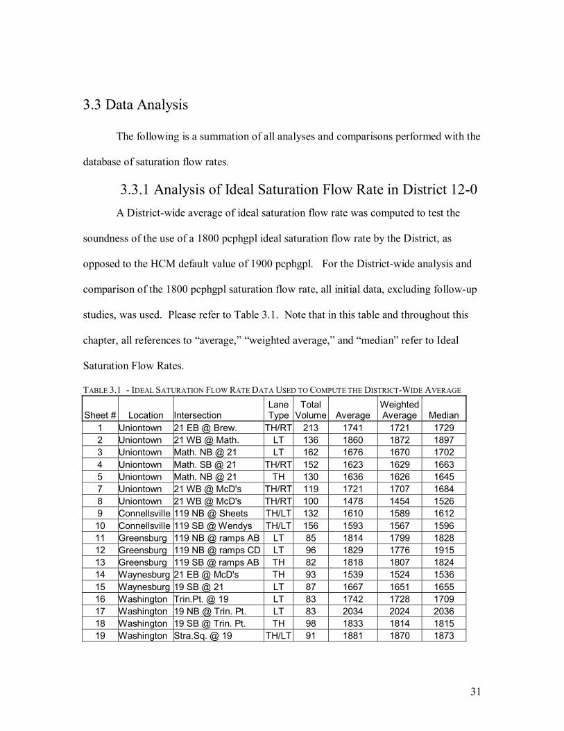
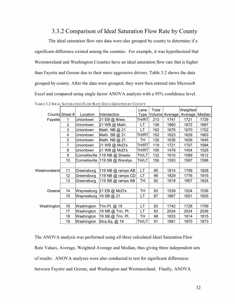
3.3 Data Analysis------------------------------------------------------------------------------ 31 3.3.1 Analysis of Ideal Saturation Flow Rate in District 12-0 ------------------------ 31 3.3.2 Comparison of Ideal Saturation Flow Rate by County -------------------------- 32

v

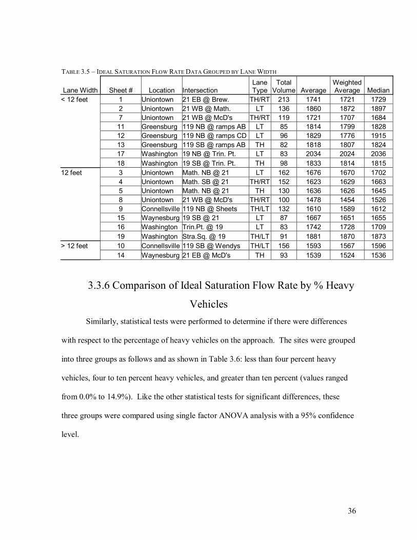
3.3.3 Comparison of Ideal Saturation Flow Rate by Lane Type ---------------------- 33 3.3.4 Comparison of Ideal Saturation Flow Rate by Approach Grade --------------- 34 3.3.5 Comparison of Ideal Saturation Flow Rate by Lane Width--------------------- 35 3.3.6 Comparison of Ideal Saturation Flow Rate by % Heavy Vehicles------------- 36 3.3.7 Comparison of Ideal Saturation Flow Rate between Rain and Dry Atmospheric Conditions----------------------------------------------------------------------------------- 37 3.3.8 Comparison of Ideal Saturation Flow Rate by Time of Day-------------------- 38

Chapter 4 - Results ----------------------------------------------------------------------------- 39

4.0 Introduction ------------------------------------------------------------------------------- 39 4.1 District -Wide Assumed Ideal Saturation Flow Rate of 1800pcphgpl -------------- 39

4.2 Ideal Saturation Flow Rate by County ------------------------------------------------- 40 4.3 Ideal Saturation Flow Rate by Lane Type.--------------------------------------------- 43

4.4 Ideal Saturation Flow Rate by Grade.-------------------------------------------------- 44 4.5 Saturation Flow Rate by Lane Width. -------------------------------------------------- 44

4.6 Ideal Saturation Flow Rate by the Percentage of Heavy Vehicles. ----------------- 46 4.7 Ideal Saturation Flow Rate for Rain vs. Dry ------------------------------------------ 47

4.8 Ideal Saturation Flow Rate by Time of day-------------------------------------------- 49 4.9 Conclusions and Recommendations ---------------------------------------------------- 50

Chapter 5 � Conclusions----------------------------------------------------------------------- 53

5.0 Conclusions-------------------------------------------------------------------------------- 53

5.1 Limitations of the Research and Recommendations for Further Research--------- 55

References---------------------------------------------------------------------------------------- 57

Appendix I --------------------------------------------------------------------------------------- 58

(Correction Factor Default Values) --------------------------------------------------------- 58

Appendix II -------------------------------------------------------------------------------------- 63

(Data reduction Summary Sheets)----------------------------------------------------------- 63

Appendix III ------------------------------------------------------------------------------------- 67

(Field collection/Data reduction sheets)----------------------------------------------------- 67

Appendix IV ------------------------------------------------------------------------------------- 95

vi

(ANOVA analysis output sheets)------------------------------------------------------------- 95

Appendix V ------------------------------------------------------------------------------------- 108

(Duncan�s Multiple Range test) ------------------------------------------------------------- 108

Vita ----------------------------------------------------------------------------------------------- 110

vii

List of Figures

FIGURE 3-1 (NAVTEQ 2003) DISTRICT 12-0 MAP .................................................22

FIGURE 3.2 (TRB, 2000) HCM SFR FIELD COLLECTION WORKSHEET .....................27

FIGURE 3.3 MODIFIED FIELD COLLECTION WORKSHEET.........................................28

FIGURE 3.3 SAMPLE DATA COLLECTION/REDUCTION SHEET...................................30

FIGURE 4.1 (DISTANCE FROM URBAN CORE VERSES IDEAL SATURATION FLOW RATE) .41

FIGURE 4.2 (RAIN DATA COMPARISON).............................................................48

FIGURE 4.3 (TIME OF DAY COMPARISON) ...........................................................50

List of Tables

TABLE 3.1 - IDEAL SATURATION FLOW RATE DATA USED TO COMPUTE THE DISTRICT-

WIDE AVERAGE........................................................................................31

TABLE 3.2 IDEAL SATURATION FLOW RATE DATA GROUPED BY COUNTY .................32

TABLE 3.3 IDEAL SATURATION FLOW DATA GROUPED BY LANE TYPE......................34

TABLE 3.4 IDEAL SATURATION FLOW RATE DATA GROUPED BY APPROACH GRADE ....35

TABLE 3.5 � IDEAL SATURATION FLOW RATE DATA GROUPED BY LANE WIDTH ........36

TABLE 3.6 � IDEAL SATURATION FLOW RATE DATA GROUPED BY PERCENT HEAVY

VEHICLES................................................................................................37

TABLE 3.7 IDEAL SATURATION FLOW RATE DATA UNDER DRY AND RAINING

CONDITIONS ............................................................................................38

TABLE 4.1 GEOGRAPHICAL COMPARISONS ANOVA SUMMARY ...............................43

TABLE 4.2 CORRECTION FACTOR ANOVA SUMMARIES.....................................46

1

CHAPTER 1 � INTRODUCTION 1.0 Introduction

The Highway Capacity Manual (HCM) (TRB, 2000) is the most commonly used

highway traffic capacity analysis tool. HCM provides the user with the theory and

methodologies to determine the capacity and level of service of a wide variety of

highway facilities, including the following (TRB, 2000):

• Urban Arterials

• Signalized Intersections

• Unsignalized Intersections

• Pedestrian facilities

• Bicycle facilities

• Rural Two-Lane Highways

• Multilane Highways

• Basic Freeway Segments

• Weaving Freeway Sections

• Ramps

• Transit facilities (e.g. terminals)

As stated, two of the key usages of HCM are to determine capacity and level of

service. Capacity is defined as the maximum number of persons or vehicles that a facility

can accommodate with reasonable safety during a specified time period (TRB, 2000). It

is generally expressed as an hourly flow rate; however, the specified time period is

typically fifteen minutes. Level of service is defined as a measure that describes

2

operational conditions within a traffic stream, generally in terms of such service measures

as speed and travel time, freedom to maneuver, traffic interruptions, and comfort and

convenience (TRB, 2000). It is generally expressed as a letter grade between A and F,

with A being near free-flow conditions, and F being over-capacity.

Engineers use the concepts of capacity and level of service in a number of ways.

One common usage is to size facilities during design. For example, the computation of

capacity and level of service can lead directly to decisions regarding the number of lanes

needed on a highway facility. Certain facility types also make specialized usage of these

concepts. For example, the level of service and capacity results for a signalized

intersection are a key input into the signal timing.

This research deals with the signalized intersection module of HCM. There are

five major steps in the computation of capacity and level of service of a signalized

intersection. They are as follows (TRB, 2000):

• Input Parameters � Gathering field data related to the geometries, traffic conditions,

and signal timings.

• Lane Grouping and Demand Flow Rate � Making adjustments to the hourly traffic

volumes to convert to fifteen minute flow rates, the deduction of right-turn on red

traffic, and the grouping of lanes with operational dependencies.

• Saturation Flow Rate � Determining the prevailing saturation flow rate, which is

defined as the flow in vehicles per hour than can be accommodated by a specified

lane group assuming that the green phase was displayed 100 percent of the time

(TRB, 2000).

3

• Capacity and Volume to Capacity Ratio � The computation of capacity for each lane

group is based on the saturation flow rate and the percentage of time the lane group

receives a green indication.

• Performance Measures � Average Control Delay per Vehicle is computed and

compared to the thresholds for each LOS.

As can be seen, the saturation flow rate is a key input when analyzing capacity, level

of service, signal timing and intersection design. The usage of a saturation flow rate that

is higher than the prevailing saturation flow rate in the field will make traffic flow appear

more efficient than it truly is in the analysis. This can result in intersections that are

under-built and / or have signal timing with green intervals and cycle lengths that are too

short. Likewise, the usage of a saturation flow rate that is too low will result in

overbuilding of intersections and motorist delays due to excessively long cycle lengths.

The model contained in HCM for predicting saturation flow rate is one in which an

ideal saturation flow rate is factored to a smaller number based on the prevailing,

presumably �non-ideal� conditions. A default value of 1900 passenger cars per hour

green per lane (pcphgpl) is provided by HCM (TRB, 2000) for the ideal saturation flow

rate. A series of factors are then provided to account for the effects of the following:

• The Number of Lanes in the Lane Group

• Lane Widths

• Heavy Vehicles

• Grade

• Parking Activity

• Bus Stops

4

• Area Type

• Lane Utilization

• Left-Turns in the Lane Group

• Right-Turns in the Lane Group

• Pedestrians that Interfere with Left-Turns

• Pedestrians and Bicyclists that Interfere with Right-Turns

As can be seen, the value used for ideal saturation flow rate has a one-to-one proportional

influence on the resultant prevailing saturation flow rate predicted by the HCM model.

Furthermore, there is uncertainty regarding the appropriateness of the default ideal

saturation flow rate provided by HCM at all geographic locations.

1.1 Problem Statement

In all signalized intersection analyses performed with HCM, the Pennsylvania

Department of Transportation (PENNDOT) District 12-0 uses an ideal saturation flow

rate of 1800 pcphgpl, which is less than the default value of 1900 pcphgpl provided by

HCM. This is to account for the less aggressive characteristics of the local drivers. The

purpose of this study is to field measure a sample of saturation flow rates, from which

ideal saturation flow rates can be computed, in District 12-0 to determine the

appropriateness of the lower ideal saturation flow rate and compare it to the distance from

the urban core within the district. This study will scientifically test this hypothesis, along

with measuring variations over the four-county District area, and variations during

different weather conditions. Furthermore, it may be possible to provide anecdotal

insight into potential shortcomings in the HCM saturation flow rate model, or the

adjustment factors used therein. One of the goals of this project is to evaluate the

5

methodology for measuring ideal saturation flow rate. The HCM provides a

methodology for measuring prevailing saturation flow rate. This methodology will be

used in conjunction with a reverse application of the HCM saturation flow model to

estimate ideal saturation flow rate. A key contribution of this work will be a qualitative

assessment of the soundness of this approach.

1.2 Project Objectives

As noted, the overall goal of the project was to determine whether PENNDOT

District 12-0 is justified in using the ideal saturation flow rate of 1800 pcphgpl. In

general, this was performed by collecting saturation flow rate data throughout the District

at locations of varying geometric make up. Data collection was also performed in

various weather conditions to check for lower saturation flow rate values as a result of

environmental conditions. Ideal saturation flow rates were then computed by using the

HCM adjustment factors to back calculate the ideal saturation flow rate from the

prevailing saturation flow rate. Statistical tests were then performed to determine if the

data supported the usage of a lower ideal saturation flow rate during normal or adverse

weather conditions. Anecdotal insight was also provided into the usage of the factors

required by the HCM model. A list of the specific research objectives is as follows:

• Review literature related to saturation flow rate, particularly the model contained in

HCM.

• Collect a statistically valid data set containing data from the four counties in

PENNDOT District 12-0, those being Fayette, Greene, Westmoreland, and

Washington Counties.

6

- Ensure in the data collection some variation in intersection geometries (i.e., grade,

lane width, etc.)

- Collect data at one location under two different weather conditions, once under

dry conditions and once in the rain.

• Conduct statistical tests to determine if there is statistical evidence that the ideal

saturation flow rate in District 12-0 is less than default value of 1900 pcphgpl.

• Conduct statistical tests to determine if there is statistical evidence of a drop in ideal

saturation flow rate during adverse weather conditions such as rain.

• Conduct statistical tests to determine if there is some variation between the individual

counties.

• Make anecdotal observations about the structure of the HCM saturation flow rate

model and its associated factors.

• Present the results, findings, and recommendations in a final report.

1.3 Organization of the Report

This chapter has provided background information, problem statement, and the

research objectives. Chapter 2 provides a literature review that focuses on the HCM

saturation flow rate model. Chapter 3 provides a description of the methodology

followed in the research. Chapter 4 presents the results of the research in detail. Chapter

5 concludes the report with a summary of the results, a description of the limitations of

the research, and ideas for further research.

7

CHAPTER 2 � LITERATURE REVIEW

2.0 Introduction

A review of literature was undertaken to critically evaluate and learn from

published research findings on the study of saturation flow rates as well as relevant

information pertaining to the validity of the data from a statistical viewpoint.

Objectives of this literature review were:

• Investigate the structure and methodology of the saturation flow rate model in HCM.

• Present the methodology for field collecting saturation flow rate that is prescribed by

HCM

• Review other published research reports related to saturation flow rates.

• Gather information related to the statistical testing of the collected data to guide the

development of the experimental plan and field data collection.

Each of these is described in a separate section as follows.

2.1 HCM Saturation Flow Rate Model Structure and Methodology

The method for determining the ideal saturation flow rate in accordance with

HCM is as follows. The saturation flow rate module is contained in the signalized

intersection module (Garber, 1999). This model provides for the computation of a

saturation flow rate for each lane group. The saturation flow rate is defined as the flow

rate in vehicles per hour that the lane group can carry if it has the green indication

continuously, that is, if g/C=1 (TRB, 2000). The saturation flow rate depends on the

ideal saturation flow rate (so), along with a number of geometric and operational

8

variables, so is equal to 1900 pcphgpl according to the HCM (TRB, 2000). The Ideal

Saturation Flow rate of 1900pcphgpl is calculated based on ideal conditions and

saturation flow headway of 1.9sec applied to the following equation.

s = 3,600/h

Where:

s = saturation flow rate (vphgpl)

h = saturation headway (sec.)

3,600 = number of seconds per hour

This ideal saturation flow is then adjusted by factors to account for the prevailing

traffic conditions to obtain the saturation flow for the lane group being considered. The

adjustment is made by introducing factors that correct for less than ideal conditions

produced by the following:

• Number of lanes

• Lane width

• Heavy vehicles in the traffic stream

• Approach grade

• Parking activity

• Buses

• Area type

• Lane utilization

• Right and left-turns

• Pedestrian and bicyclist interference with turning vehicles

The prevailing saturation flow rate is given by the following equation from HCM

(TRB, 2000):

9

s = (so)(N)(fw)(fHV )(fg)(fp)(fa)(fbb)(fLU)(fRT)(fLT)(fLpb)(fRpb)

Where

s = saturation flow rate for the subject lane group, expressed as a total for all lanes

in the lane group under prevailing conditions (vphg)

so = ideal saturation flow rate per lane, usually taken as 1900 (vphg/ln)

N = number of lanes in lane group

fw = adjustment factor for lane width

fHV = adjustment factor for heavy vehicle in the traffic in the traffic stream

fg = adjustment factor for approach grade

fp = adjustment factor for the existence of parking lane adjacent to the lane group

and the parking activity on that lane

fa = adjustment factor for area type (for Central Business District or CBD, 0.90;

for all other areas, 1.00)

fbb = adjustment factor for the blocking effect of local buses stopping within the

intersection area

fLu = adjustment factor for lane utilization

fRT = adjustment factor for right turns in the lane groups

fLT = adjustment factor for the left turns in the lane group

fLpb = pedestrian adjustment factor for the left-turns movements

fRpb = pedestrian-bicycle adjustment factor for the right-turns movements.

Each of the adjustment factors is discussed in detail below typical values and the

equations used to compute the factors can be seen in Appendix I.

10

Lane Width Adjustment Factor, fw. This factor depends on the average width

of the lanes in a group. It is used to account for both the reduction in saturation flow

rates when lane widths are less than 12 ft and the increase in saturation flow rates when

lane widths are greater than 12 ft. The adjustment factors are obtained from Appendix I

(TRB, 2000). Lane width factors should not be computed for lanes less than 8 ft wide. A

lane width of 12 ft. would result in an adjustment factor of one, which would have no

effect on saturation flow rate. A lane width less than 12 ft. results in a factor less than

one, thus lowering saturation flow rate, and a lane width greater than 12 ft. results in a

factor that is greater than one, thus increasing saturation flow rate.

Heavy Vehicle Adjustment Factor, fHV. The heavy vehicle adjustment factor is

related to the percentage of heavy vehicles in the specified lane group. This factor

corrects for the additional delay and reduction in saturation flow rate due to the presence

of heavy vehicles in the traffic stream. Note that a heavy vehicle is defined as any

vehicle that has more than four wheels touching the pavement (TRB, 2000). The

additional delay and reduction in saturation flow are due mainly to the difference

between the operational capabilities of the heavy vehicles and passenger cars and the

additional space taken up by heavy vehicles. The appropriate factor is selected from

Appendix I (TRB, 2000).

Grade Adjustment Factor, fg. This factor is related to the gradient of the

approach being considered. It is used to correct for the effect of gradients on the speed of

vehicles, including both passenger cars and heavy vehicles. This effect is different for

up-grade and down-grade conditions; therefore, the direction of the grade is also taken

into consideration as shown in Appendix I (TRB, 2000). Note that upgrades yield factors

11

that are less than one, while downgrades are associated with factors that are greater than

one.

Parking Adjustment Factor, fp. On-street parking within 250 ft upstream of the

stop bar of an intersection causes friction between parking and through vehicles, which

results in a reduction of the saturation flow rate. This effect is corrected for by using a

parking adjustment factor, which can be found in Appendix I (TRB, 2000). This factor

depends on the number of lanes in a lane group and the number of parking maneuvers per

hour. Examination of the parking adjustment factors reveals that the higher the number

of lanes in a given lane group, the less effect parking has on the saturation flow rate.

Conversely, the higher the number of parking maneuvers, the greater the effect. In

determining these factors, it is assumed that each parking maneuver (either in or out)

blocks traffic on the adjacent lane group for an average duration of 18 sec. It should be

noted that when the number of parking maneuvers per hour is greater than 180, a

practical limit of 180 should be used. This adjustment factor should be applied only to

the lane group immediately adjacent to the parking lane. When parking occurs on both

sides of a single lane group, the sum of the number of parking maneuvers on both of sides

should be used.

Area Type Adjustment Factor, fa. The general types of activities in the area at

which the intersection is located have a significant effect on speed and therefore on

saturation flow rate on an approach. For example, because of the complexity of

intersections located in areas with typical central business district characteristics, such as

frequent parking maneuvers, narrow streets, and high pedestrian activities, these

intersections operate less efficiently than intersections at other areas. This is corrected

12

for by using the area type adjustment factor fa, which is 0.90 for a central business district

(CBD) and 1.0 for all areas not designated as CBD�s (TRB 2000)

Bus Blockage Adjustment Factor, fbb. When buses have to stop in a travel lane

to discharge or pick up passengers, all of the vehicles immediately behind the bus will

also have to stop. This results in a decrease in the maximum volume that can be served

by that lane. This effect is corrected for by using the bus blockage adjustment factor,

which is related to the number of buses in an hour that stop in the travel lane, within 250

ft upstream or downstream of the stop line, as well as the number of lanes in the lane

group. The factors developed in HCM (TRB, 2000) assume an average blockage time of

14.4 sec during a green indication. These values can be seen in Appendix I (TRB, 2000).

Lane Utilization Adjustment Factor, fLu. The lane utilization factor is used to

adjust the ideal saturation flow rate to account for the unequal utilization of the lanes in a

lane group. When a lane group has more than one lane serving a movement (e.g. two

lanes for through moving traffic) the lane utilization factor is obtained from the following

equation as:

fLui = (vgi) / (vgLiNi)

Where:

fLui = lane utilization adjustment factor for lane group i

vgi = unadjusted demand flow rate for lane group i

vgLi = unadjusted demand flow rate on the single lane of group I with the highest volume

Ni = number of lanes in lane group i

13

It is recommended that actual field data be used for computing fLui. Values shown

in Appendix I, however, can be used as default values when field information is not

available (TRB, 2000).

Right-Turn Adjustment Factor, fRT. This factor accounts for the effect of right-

turning vehicles on saturation flow rate. It depends on the right-turn protection provided

in the phase plan (protected, permitted, or protected plus permitted), the conflicting

pedestrian volume, and the proportion of right-turning vehicles that use the protected

portion of the protected-plus-permitted phase. This portion can be determined from a

field study or, alternatively, can be estimated from the signal timing by assuming that the

proportions of the right-turning phase are approximately equal. The right-turning volume

may also be reduced if right-turn-on-red is always allowed, by subtracting the number of

vehicles that turn during the red phase from the total right-turn volume. Appendix I gives

the right turn adjustment factors (TRB, 2000).

Left-Turn Adjustment Factor, fLT. This adjustment factor is used to account for

the fact that left-turn movements take more time to execute than through movements.

The values of this factor also depends on the type of phasing (protected, permitted, or

protected-plus-permitted), the type of lane used for the left-turns (exclusive or shared

lane), and the proportion of left-turn vehicles using a shared lane. Appendix I gives left-

turn adjustment factors (TRB, 2000).

Adjustment for Pedestrians and Bicyclists fLpb, fRpb. The procedure to determine

the left-turn pedestrian-bicycle factor, f Lpb, and the right-turn pedestrian-bicycle

adjustment factor, fRpb, consist of four steps. The first step is to determine average

pedestrian occupancy, which only accounts for the pedestrian effect. Next, the relevant

14

conflict zone occupancy, which accounts for both pedestrian and bicycle effects is

determined. Relevant conflict zone occupancy takes into account whether other traffic is

also in conflict (e.g. adjacent bicycle flow for the case of right-turns or opposing vehicle

flow for the case of left turns). In either case, adjustments to the initial occupancy are

made. The portion of green time in which the conflict zone is occupied is determined as

a function of the relevant occupancy and the number of receiving lanes for the turning

vehicles.

The proportion of right-turns using the protected sequence of a protected-plus-

permitted phase is also needed. This proportion should be determined by field

observation, but a gross estimate can be made from the signal timing by assuming that the

proportion of the right-turning vehicles using the protected phase is approximately equal

to the proportion of the turning phase that is protected. If PRTA = 1.0 (that is, the right

turn is completely protected from conflicting pedestrian), a pedestrian volume of zero

should be used.

Finally, the saturation flow rate adjustment factor is calculated from the final

occupancy on the basis of the turning movement protection status and the percent of

turning traffic in the lane group. All information required to compute this factor from the

appropriate field data is provided in Appendix I (TRB, 2000).

In conclusion, these factors are used in the HCM saturation flow rate model to

account for less than ideal conditions with prevailing traffic and intersection conditions to

compute prevailing saturation flow rate. They will be used in reverse during this research,

as the prevailing saturation flow rate will be measured and factored up to the ideal

15

saturation flow rate based on the prevailing conditions. Note that all factors not used

later in the study were not present at the data collection location.

2.2 HCM-Prescribed Methodology for Field Collecting Saturation

Flow Rate Data

To eliminate variation in the field collection of saturation flow rate data, HCM

(TRB, 2000) prescribes a detailed procedure for its collection. The methodology is

illustrated by the following example (TRB, 2000).

This example describes a single-lane saturation flow survey. A two-person field crew

is recommended, however, one person will suffice. The field notes and tasks identified in

the following section must be adjusted accordingly.

1. General Tasks

a. Record the area type and width and grade of the lane being studied.

b. Fill out the survey identification data shown in Figure 3.2 completely.

c. Select an observation point where the stop line for the surveyed lane and

corresponding signal heads are clearly visible.

d. The reference point is normally the stop line. Vehicles should consistently

stop behind this line. When a vehicle crosses it unimpeded, it has entered

the intersection conflict space for the purpose of saturation flow rate

measurement. Left- or right-turning vehicles yielding to opposing through

traffic or yielding to pedestrians are not recorded until they proceed

through the opposing traffic.

2. Recorder Tasks

a. Note the last vehicle in the stopped queue when the signal turns green.

16

b. Describe the last vehicle to the timer.

c. Note on the worksheet which vehicles are heavy vehicles and which

vehicles turn left or right.

d. Record the time called out by the timer.

3. Timer tasks

a. Start the stopwatch at the beginning of the green and notify the recorder.

b. Count aloud each vehicle in the queue as its rear axle crosses the stop line.

c. Call out the time of the fourth, tenth, and last vehicle in the queue.

d. If queued vehicles are still entering the intersection at the end of the green,

call out �saturation through the end of green-last vehicle was number

XX.�

Note any unusual events that may have influenced the saturation flow rate, such

as buses, stalled vehicles, and unloading trucks. The period of saturation flow rate that

begins when the rear axle of the fourth vehicle in the queue crosses the stop line or

reference point and ends when the rear axle of the last queued vehicle at the beginning of

the green time crosses the stop line.

Measurements are taken cycle by cycle. To reduce the data for each cycle, the

time recorded for the fourth vehicle is subtracted from the time recorded for the last

vehicle in the queue. This value is total headway for (n-4) vehicles, where n is the

number of the last vehicle surveyed (this may not be the last vehicle in the queue). The

total headway is divided by (n-4) to obtain the average headway per vehicle under

saturation flow. The saturation flow rate is 3,600 divided by this value. For example, if

17

the time for the fourth vehicle was observed as 10.2 sec and the time for the 14th and last

vehicle surveyed was 36.5 sec, the average saturation headway per vehicle would be

(36.5-10.2) / (14-4) = 26.3 / 10 = 2.63 sec/veh

And the prevailing saturation flow rate in that cycle would be

3,600 / 2.63 = 1,369 vphgpl

In order to obtain a statistically significant value, a minimum of 15 signal cycles with

more than 8 vehicles in the initial queue is usually needed (TRB, 2000). An average of

the saturation flow rate values in individual cycles represents then the prevailing local

saturation flow rate for the surveyed lane. The percentage of heavy vehicles and turning

vehicles in the sample used in the computations should be determined and noted for

reference.

2.3 Other Related Saturation Flow Rate Literature

(McMahon, Krane, & Federico, 1997) conducted a similar study in the state of

Florida, in which they performed a study to test for geographical differences in saturation

flow rate among the five south Florida counties that make up the Florida Department of

Transportation (FDOT) District Four. These five counties were Broward, Palm Beach,

Martin, St. Lucie and Indian River. These counties varied in their level of development

from urban to rural much like PENNDOT District 12-0. FDOT hypothesized that there

were variations in saturation flow rates between the five counties and desired to develop a

database to support localized saturation flow rate assumptions used in traffic operations

analysis. The same HCM methodology was used for collecting the field data with the

exception of the minimum number of vehicles required in each queue. The FDOT study

18

used a minimum of six vehicles due to a change in the HCM from the second to the third

edition. Some of the conclusions of their study were as follows:

• Contrary to original hypothesis that a geographical difference exists among saturation

flow rates throughout District Four, it was established that more significant variation

was exhibited by the number of through lanes per approach.

• There was substantial similarity of saturation flow rates among roadways that have

three through approach lanes.

• It was inconclusive whether there was a geographical difference among single-lane

and two-lane approaches throughout the District.

Also, a few of the following recommendations from the study are listed below:

• An examination of the entire data set ranked in the order of decreasing saturation flow

rates, by cycle, and its comparison with other research and the HCM value of 1900

could provide valuable insight regarding the �true� south Florida saturation flow rate.

• A more thorough analysis of the impact of heavy vehicles based on the percentage of

trucks may provide additional insight into truck adjustment factors for South Florida.

• Analysis of shared through/turn-lane characteristics relative to percent turns could

provide additional information relative to adjustment factors for shared lanes.

2.4 Literature Related to Statistical Procedures

The goal of this project was to design and conduct an experiment to test the validity

of the usage of a lower ideal saturation flow in PENNDOT District 12-0. As such, some

background information on statistical testing and experimental design was needed. This

section provides the necessary background to establish the experimental design and

analysis that is described in Chapter 3.

19

(Lum,1991) states, in Statistical Shortcomings in Traffic Studies, �Over the years, the

Federal Highway Administration (FHWA) has been receiving more and more research

reports in which the authors use statistical techniques of analysis of variance and

regression analysis. Many of these studies are flawed due to a lack of understanding of

the assumptions underlying these statistical techniques. Consequently, the findings and

conclusions presented in the reports may be open to questions and challenge.

Furthermore, from (Walpole et al., 1998), a few statistical tests that will prove the

worth of the data are as follows:

- ANOVA analysis

- Duncan�s Multiple Range Test

Analysis-of-Variance (ANOVA) is used to test variation in F-distribution between

two or more sample populations. This test is conducted by comparing variability within a

sample to variability between samples, in this case using a 95% confidence interval. For

example, ANOVA analysis can be performed between sets of ideal saturation flow rates

collected in two different counties to determine whether there is a statistically

significantly difference. ANOVA analysis can compare two populations of different

sample size, which is useful in this study because an equal number of ideal saturation

flow rate observations were not made in each county.

A second test that can be performed is the Duncan�s multiple-range test. This

procedure is based on the general notion of studentized range along with a normal

distribution. The range of any subset of p sample means must exceed a certain value

before any of the p means are found to be different, this test was conducted using a 95%

20

confidence interval with 19 degrees of freedom. This test proves to be useful here to

compare all four counties to each other instead of a one on one basis.

2.5 Concluding Remarks

This chapter has investigated important literature and background information

needed to support the research goals of this project. Important observations relative to

the research experiment design were made and will be directly incorporated into the

project methodology, to be described in Chapter 3.

21

Chapter 3 - Methodology

3.0 Introduction

This chapter describes the methodology followed in the execution of this research.

Each primary step in the research is covered in a separate section. Section 3.1 describes

the data collection sites, the dates of the data collection, and any important circumstances,

under which the data were collected, (e.g., rain). Section 3.2 describes the data reduction

and storage, and describes the process under which the prevailing saturation flow rates

were used to estimate ideal saturation flow rates. Section 3.3 describes the data analysis

that was performed, including the analysis of the 1800 pcphgpl district-wide ideal

saturation flow rate, the comparison of ideal saturation flow rates by county, the

comparison of ideal saturation flow rates by other site characteristics, and the analysis of

adverse weather conditions on ideal saturation flow rate.

3.1 Data Collection

Data were collected in the four counties comprising Pennsylvania Department of

Transportation - Engineering District 12. These four counties are located in southwestern

Pennsylvania and are as follows: Fayette, Greene, Westmoreland, and Washington. The

Pittsburgh metropolitan area is just to the north of the study area, and its suburban area

spills into both Westmoreland and Washington Counties. See Figure 3-1 for a Site Map

of the area including the locations of data collection.

22

Figure 3-1 (Navteq 2003) District 12-0 Map

The locations of data collection were as follows:

- Uniontown and Connellsville in Fayette County

- Greensburg in Westmoreland County

- Waynesburg in Greene County

23

- Washington in Washington County

These locations vary in driver characteristics, as the Washington and Greensburg

sites are more indicative of suburban Pittsburgh drivers, while the Fayette and Greene

County sites are more indicative of rural drivers. As such, comparisons can be made

between presumably aggressive and less-aggressive drivers. With the exception of

Connellsville, all municipalities were county seats. Furthermore, these locations were

selected because they had signalized intersections that had significant queuing for an

extended duration during the peak periods. This was required to conduct the saturation

flow rate study and obtain an adequate sample.

At each selected signalized intersection, lanes were selected for study with a wide

range of characteristics to enable the comparison between correction factors such as lane

type, lane width, and grade. Data were collected at the following lanes / signalized

intersections on the following dates:

- May 29-2002 (Wednesday)

Uniontown, Intersection of PA 21 and Brewer Drive:

• PA 21 Eastbound shared through (TH) & right (RT)

Uniontown, Intersection of PA 21 at Matthew Drive and US 40 / 119 Ramps:

• PA 21 Westbound left (LT) Only

• Northbound Ramps LT Only

• Southbound Matthew Drive shared TH and RT

• Northbound Ramps 40 TH Only

- June 4, 2002 (Tuesday)

Waynesburg, Intersection of US 19 and PA 21:

24

• US 19 southbound LT Only

Waynesburg, Intersection of PA 21 and McDonalds:

• PA 21 Eastbound TH Only

- June 5, 2002 (Wednesday)

Uniontown, Intersection of PA 21 at Matthew Drive and US 40 / 119 Ramps:

• Northbound from 40 LT Only (hard rain)

Uniontown, @ intersection of PA 21 and Work Parkway:

• PA 21 Westbound TH Only

• PA 21 Eastbound shared TH and RT

- June 10,2002 (Monday)

Connellsville, Intersection of US 119 SB and PA 711

• US 119 Southbound shared LT and TH

Connellsville, Intersection of US 119 NB and PA 711

• US 119 Northbound shared LT and TH

- June 12, 2002 (Wednesday)

Greensburg, Intersection of US 119 and US 30 Ramps

• US 119 Northbound LT Only (to US 30 Westbound)

• US 119 Southbound TH Only

• US 119 Northbound LT Only (to US 30 Eastbound)

- July 8, 2002 (Monday)

Washington, Intersection of US 19 and Trinity Point / Strabane Square access

• Westbound from Strabane Square shared LT and TH

• US 19 Southbound TH Only (right lane)

25

• Eastbound from Trinity Point LT Only

• US 19 Northbound LT Only

- October 10 2002 (Thursday)

Uniontown, @ intersection of PA 21 at Matthew Drive and US 40 / 119 Ramps:

(All rain data)

• PA 21 Westbound LT Only

• Northbound Ramps LT Only

• Southbound Matthew Drive shared TH and RT

- October 23, 2002 (Wednesday)

Uniontown, @ intersection of PA 21 at Matthew Drive and US 40 / 119 Ramps:

(Time of day study)

• Northbound Ramps LT Only (In 1 hour increments from 12:00 to

5:00)

As can be seen, the majority of the data collection was performed in June 2002,

with the exception of a few days of data collection in May, July, and October of that year.

Following preliminary data reduction, a follow-up was performed in mid-October to

address some initial findings. The October 11th collection was done at repeat location

while raining to compare results between the two scenarios. In addition, the October 23rd

collection was done at a repeat location studying the same lane from 12:00 pm to 5:00 pm

to check for differences in data for varying time of day.

The data collection was performed in accordance with the Highway Capacity

Manual 2000 (TRB, 2000) by one person and was as follows. The saturation flow rate

26

was measured by recording the time and number of vehicles crossing a stop bar from a

standing queue when the signal indication turned green. A like point on all vehicles was

used (rear axle) to start and stop the timing to eliminate any variation in the data

collection. There was a minimum of eight vehicles required in the standing queue to

collect the data. Time was recorded from the fourth vehicle in the queue to the last.

HCM recommended a minimum of 15 cycles to be recorded for each approach to achieve

a representative sample. In this study, 20 cycles were sampled to further ensure the

validity of the sample. Shown below are field collection sheets from HCM in Figure 3.2,

as well as a simplified collection sheet used in this study in Figure 3.3. Figure 3.3 may

vary from the HCM format below due to site specific features. If field measurements

were to include the grade and lane dimensions, they were also recorded on the field

observation sheet.

27

Figure 3.2 (TRB, 2000) HCM SFR Field Collection Worksheet

28

Figure 3.3 Modified Field collection Worksheet North/South: City:

East/West: State: Approach studied: Technician:

Weather: Time: Pavement Condition: Date:

# Of Counts

Elapsed Time (sec.)

Total # of vehicles

# Of heavy

vehicles # Of R/L

Turns 1 2 3 4 5 6 7 8 9 10 11 12 13 14 15 16 17 18 19 20

3.2 Data Reduction

From the raw data which can be seen in Appendix II and III, the prevailing

saturation flow rate was computed for each cycle, then aggregated using both an

unweighted and weighted (according to number of vehicles) average. Concurrently, all

geometric information was obtained for the sample intersections using the permit

drawings that were provided by PENNDOT. Permit drawings are engineering drawings

29

of the intersection that contain pertinent signal-related design features, including

approach grades and lane widths, which were critical to this study. Then using the

average field-measured saturation flow rate and the adjustment factors from HCM that

corresponded to each non-ideal condition, the ideal saturation flow rate was computed.

Additionally, the standard deviation, variance, median, and coefficient of variation were

also computed in the prevailing saturation flow rate to gauge the variability of the data

and for use in subsequent statistical analyses. See Figure 3.3 for a sample computation

sheet from Microsoft Excel.

30

Figure 3.3 Sample Data Collection/Reduction Sheet North/South:Brewer Drive City: Uniontown

East/West:PA 21 State: Pa. Approach studied: PA 21 EB TH / RT Technician: BMD

Weather:82, clear Time: 1:07-2:10pm Pavement Condition:Dry Date: 5/29/02

# Of Counts Elapsed Time (sec.) Total # of vehicles # Of heavy

vehicles # Of Rt. Turns Calculated SFR

1 16.28 8 0 1 1769.04 2 35.25 16 1 1 1634.04 3 22.69 9 2 0 1427.94 4 26.01 10 2 2 1384.08 5 30.22 10 2 2 1191.26 6 27.15 8 2 0 1060.77 7 23.85 13 0 0 1962.26 8 24.25 11 0 0 1632.99 9 21.22 9 0 0 1526.86 10 25.03 12 1 1 1725.93 11 29.16 13 2 0 1604.94 12 17.02 8 0 1 1692.13 13 25.38 10 2 1 1418.44 14 21.94 10 0 2 1640.84 15 26.75 11 1 1 1480.37 16 28.69 10 2 1 1254.79 17 28.68 12 2 0 1506.28 18 29.15 12 2 0 1481.99 19 17.91 9 0 0 1809.05 20 28.35 12 1 0 1523.81

Sum: 504.98 213 22 13 30727.82

g = -3% % Heavy veh.: 10.3 Lw = 11' % Rt turns: 6.1 Ideal:

Average SFR: 1536.39 1741

Weighted Average

SFR: 1518.48 1721 Standard deviation: 215.85

Coefficient of

Variation: 14.21 Median: 1525.34 1729 Variance: 46591.33

31

3.3 Data Analysis

The following is a summation of all analyses and comparisons performed with the

database of saturation flow rates.

3.3.1 Analysis of Ideal Saturation Flow Rate in District 12-0 A District-wide average of ideal saturation flow rate was computed to test the

soundness of the use of a 1800 pcphgpl ideal saturation flow rate by the District, as

opposed to the HCM default value of 1900 pcphgpl. For the District-wide analysis and

comparison of the 1800 pcphgpl saturation flow rate, all initial data, excluding follow-up

studies, was used. Please refer to Table 3.1. Note that in this table and throughout this

chapter, all references to �average,� �weighted average,� and �median� refer to Ideal

Saturation Flow Rates.

TABLE 3.1 - IDEAL SATURATION FLOW RATE DATA USED TO COMPUTE THE DISTRICT-WIDE AVERAGE

Sheet # Location Intersection Lane Type

Total Volume Average

Weighted Average Median

1 Uniontown 21 EB @ Brew. TH/RT 213 1741 1721 1729 2 Uniontown 21 WB @ Math. LT 136 1860 1872 1897 3 Uniontown Math. NB @ 21 LT 162 1676 1670 1702 4 Uniontown Math. SB @ 21 TH/RT 152 1623 1629 1663 5 Uniontown Math. NB @ 21 TH 130 1636 1626 1645 7 Uniontown 21 WB @ McD's TH/RT 119 1721 1707 1684 8 Uniontown 21 WB @ McD's TH/RT 100 1478 1454 1526 9 Connellsville 119 NB @ Sheets TH/LT 132 1610 1589 1612 10 Connellsville 119 SB @ Wendys TH/LT 156 1593 1567 1596 11 Greensburg 119 NB @ ramps AB LT 85 1814 1799 1828 12 Greensburg 119 NB @ ramps CD LT 96 1829 1776 1915 13 Greensburg 119 SB @ ramps AB TH 82 1818 1807 1824 14 Waynesburg 21 EB @ McD's TH 93 1539 1524 1536 15 Waynesburg 19 SB @ 21 LT 87 1667 1651 1655 16 Washington Trin.Pt. @ 19 LT 83 1742 1728 1709 17 Washington 19 NB @ Trin. Pt. LT 83 2034 2024 2036 18 Washington 19 SB @ Trin. Pt. TH 98 1833 1814 1815 19 Washington Stra.Sq. @ 19 TH/LT 91 1881 1870 1873

32

3.3.2 Comparison of Ideal Saturation Flow Rate by County The ideal saturation flow rate data were also grouped by county to determine if a

significant difference existed among the counties. For example, it was hypothesized that

Westmoreland and Washington Counties have an ideal saturation flow rate that is higher

than Fayette and Greene due to their more aggressive drivers. Table 3.2 shows the data

grouped by county. After the data were grouped, they were then entered into Microsoft

Excel and compared using single factor ANOVA analysis with a 95% confidence level.

TABLE 3.2 IDEAL SATURATION FLOW RATE DATA GROUPED BY COUNTY

County Sheet # Location Intersection Lane Type

Total Volume Average

Weighted Average Median

Fayette 1 Uniontown 21 EB @ Brew. TH/RT 213 1741 1721 1729 2 Uniontown 21 WB @ Math. LT 136 1860 1872 1897 3 Uniontown Math. NB @ 21 LT 162 1676 1670 1702 4 Uniontown Math. SB @ 21 TH/RT 152 1623 1629 1663 5 Uniontown Math. NB @ 21 TH 130 1636 1626 1645 7 Uniontown 21 WB @ McD's TH/RT 119 1721 1707 1684 8 Uniontown 21 WB @ McD's TH/RT 100 1478 1454 1526 9 Connellsville 119 NB @ Sheets TH/LT 132 1610 1589 1612 10 Connellsville 119 SB @ Wendys TH/LT 156 1593 1567 1596

Westmoreland 11 Greensburg 119 NB @ ramps AB LT 85 1814 1799 1828 12 Greensburg 119 NB @ ramps CD LT 96 1829 1776 1915 13 Greensburg 119 SB @ ramps AB TH 82 1818 1807 1824

Greene 14 Waynesburg 21 EB @ McD's TH 93 1539 1524 1536 15 Waynesburg 19 SB @ 21 LT 87 1667 1651 1655

Washington 16 Washington Trin.Pt. @ 19 LT 83 1742 1728 1709 17 Washington 19 NB @ Trin. Pt. LT 83 2034 2024 2036 18 Washington 19 SB @ Trin. Pt. TH 98 1833 1814 1815 19 Washington Stra.Sq. @ 19 TH/LT 91 1881 1870 1873

The ANOVA analysis was performed using all three calculated Ideal Saturation Flow

Rate Values, Average, Weighted Average and Median, thus giving three independent sets

of results. ANOVA analyses were also conducted to test for significant differences

between Fayette and Greene, and Washington and Westmoreland. Finally, ANOVA

33

analyses were performed to test for significant differences between the combination of

Fayette and Greene (rural counties) and the combination of Washington and

Westmoreland (urban counties). In addition, Duncan�s multiple-range test was

performed using the weighted averages between the four counties. This test was

conducted to add an additional method for validating the findings.

3.3.3 Comparison of Ideal Saturation Flow Rate by Lane

Type The ideal saturation flow rate data were then grouped according to lane type.

Three lane types were sample in this study: exclusive left-turn lanes, exclusive through

lanes, and shared through and right or left-turn lanes. The grouped data are shown in

Table 3.3. It was hypothesized that if a significant difference emerged among the various

lane types, there might be an indication that the lane group factors in HCM were flawed.

Single factor ANOVA analysis was then performed to check the hypothesis using a 95%

confidence level.

34

TABLE 3.3 IDEAL SATURATION FLOW DATA GROUPED BY LANE TYPE

Lane type Sheet # Location Intersection Lane Type

Total Volume Average

Weighted Average Median

Left turn only 2 Uniontown 21 WB @ Math. LT 136 1860 1872 1897 3 Uniontown Math. NB @ 21 LT 162 1676 1670 1702 11 Greensburg 119 NB @ ramps AB LT 85 1814 1799 1828 12 Greensburg 119 NB @ ramps CD LT 96 1829 1776 1915 15 Waynesburg 19 SB @ 21 LT 87 1667 1651 1655 16 Washington Trin.Pt. @ 19 LT 83 1742 1728 1709

17 Washington 19 NB @ Trin. Pt. LT 83 2034 2024 2036 Thru only 5 Uniontown Math. NB @ 21 TH 130 1636 1626 1645

13 Greensburg 119 SB @ ramps AB TH 82 1818 1807 1824 14 Waynesburg 21 EB @ McD's TH 93 1539 1524 1536

18 Washington 19 SB @ Trin. Pt. TH 98 1833 1814 1815 Thru and 1 Uniontown 21 EB @ Brew. TH/RT 213 1741 1721 1729

(Right or left) 4 Uniontown Math. SB @ 21 TH/RT 152 1623 1629 1663 7 Uniontown 21 WB @ McD's TH/RT 119 1721 1707 1684

8 Uniontown 21 WB @ McD's TH/RT 100 1478 1454 1526 9 Connellsville 119 NB @ Sheets TH/LT 132 1610 1589 1612 10 Connellsville 119 SB @ Wendys TH/LT 156 1593 1567 1596 19 Washington Stra.Sq. @ 19 TH/LT 91 1881 1870 1873

3.3.4 Comparison of Ideal Saturation Flow Rate by Approach

Grade Similar to the �lane type� comparisons that were made, comparisons were also

made according to approach grade. Sites were grouped into three categories as shown in

Table 3.4: downgrades, upgrades, and level (values ranged from -8.0% to +6.7%). It was

hypothesized that if a significant difference emerged, the approach grade factors in HCM

might be flawed. Again, the test was performed using single factor ANOVA.

35

TABLE 3.4 IDEAL SATURATION FLOW RATE DATA GROUPED BY APPROACH GRADE

Grade Sheet # Location Intersection Lane Type

Total Volume Average

Weighted Average Median

Downgrade 1 Uniontown 21 EB @ Brew. TH/RT 213 1741 1721 1729 2 Uniontown 21 WB @ Math. LT 136 1860 1872 1897 4 Uniontown Math. SB @ 21 TH/RT 152 1623 1629 1663 8 Uniontown 21 WB @ McD's TH/RT 100 1478 1454 1526 13 Greensburg 119 SB @ ramps AB TH 82 1818 1807 1824 14 Waynesburg 21 EB @ McD's TH 93 1539 1524 1536 16 Washington Trin.Pt. @ 19 LT 83 1742 1728 1709 17 Washington 19 NB @ Trin. Pt. LT 83 2034 2024 2036

19 Washington Stra.Sq. @ 19 TH/LT 91 1881 1870 1873 Level 7 Uniontown 21 WB @ McD's TH/RT 119 1721 1707 1684

9 Connellsville 119 NB @ Sheets TH/LT 132 1610 1589 1612 10 Connellsville 119 SB @ Wendys TH/LT 156 1593 1567 1596

12 Greensburg 119 NB @ ramps CD LT 96 1829 1776 1915 Upgrade 3 Uniontown Math. NB @ 21 LT 162 1676 1670 1702

5 Uniontown Math. NB @ 21 TH 130 1636 1626 1645 11 Greensburg 119 NB @ ramps AB LT 85 1814 1799 1828 15 Waynesburg 19 SB @ 21 LT 87 1667 1651 1655

18 Washington 19 SB @ Trin. Pt. TH 98 1833 1814 1815

3.3.5 Comparison of Ideal Saturation Flow Rate by Lane

Width To investigate the HCM correction factor for lane width using ANOVA analysis,

the ideal saturation flow rate data were grouped into three categories: lane widths less

than 12 feet, equal to 12 feet, and greater than 12 feet (values ranged from 10 feet to 14

feet). These are shown in Table 3.5. Single factor ANOVA analysis was then used to

compare the three categories.

36

TABLE 3.5 � IDEAL SATURATION FLOW RATE DATA GROUPED BY LANE WIDTH

Lane Width Sheet # Location Intersection Lane Type

Total Volume Average

Weighted Average Median

< 12 feet 1 Uniontown 21 EB @ Brew. TH/RT 213 1741 1721 1729 2 Uniontown 21 WB @ Math. LT 136 1860 1872 1897 7 Uniontown 21 WB @ McD's TH/RT 119 1721 1707 1684 11 Greensburg 119 NB @ ramps AB LT 85 1814 1799 1828 12 Greensburg 119 NB @ ramps CD LT 96 1829 1776 1915 13 Greensburg 119 SB @ ramps AB TH 82 1818 1807 1824 17 Washington 19 NB @ Trin. Pt. LT 83 2034 2024 2036 18 Washington 19 SB @ Trin. Pt. TH 98 1833 1814 1815 12 feet 3 Uniontown Math. NB @ 21 LT 162 1676 1670 1702 4 Uniontown Math. SB @ 21 TH/RT 152 1623 1629 1663 5 Uniontown Math. NB @ 21 TH 130 1636 1626 1645 8 Uniontown 21 WB @ McD's TH/RT 100 1478 1454 1526 9 Connellsville 119 NB @ Sheets TH/LT 132 1610 1589 1612 15 Waynesburg 19 SB @ 21 LT 87 1667 1651 1655 16 Washington Trin.Pt. @ 19 LT 83 1742 1728 1709 19 Washington Stra.Sq. @ 19 TH/LT 91 1881 1870 1873 > 12 feet 10 Connellsville 119 SB @ Wendys TH/LT 156 1593 1567 1596 14 Waynesburg 21 EB @ McD's TH 93 1539 1524 1536

3.3.6 Comparison of Ideal Saturation Flow Rate by % Heavy

Vehicles Similarly, statistical tests were performed to determine if there were differences

with respect to the percentage of heavy vehicles on the approach. The sites were grouped

into three groups as follows and as shown in Table 3.6: less than four percent heavy

vehicles, four to ten percent heavy vehicles, and greater than ten percent (values ranged

from 0.0% to 14.9%). Like the other statistical tests for significant differences, these

three groups were compared using single factor ANOVA analysis with a 95% confidence

level.

37

TABLE 3.6 � IDEAL SATURATION FLOW RATE DATA GROUPED BY PERCENT HEAVY VEHICLES % Heavy Vehicle Sheet # Location Intersection

Lane Type

Total Volume Average

Weighted Average Median

< 4% 2 Uniontown 21 WB @ Math. LT 136 1860 1872 1897 4 Uniontown Math. SB @ 21 TH/RT 152 1623 1629 1663 5 Uniontown Math. NB @ 21 TH 130 1636 1626 1645 8 Uniontown 21 WB @ McD's TH/RT 100 1478 1454 1526 10 Connellsville 119 SB @ Wendys TH/LT 156 1593 1567 1596 13 Greensburg 119 SB @ ramps AB TH 82 1818 1807 1824 14 Waynesburg 21 EB @ McD's TH 93 1539 1524 1536 15 Waynesburg 19 SB @ 21 LT 87 1667 1651 1655 16 Washington Trin.Pt. @ 19 LT 83 1742 1728 1709 17 Washington 19 NB @ Trin. Pt. LT 83 2034 2024 2036 18 Washington 19 SB @ Trin. Pt. TH 98 1833 1814 1815

19 Washington Stra.Sq. @ 19 TH/LT 91 1881 1870 1873 4% to 10% 7 Uniontown 21 WB @ McD's TH/RT 119 1721 1707 1684

9 Connellsville 119 NB @ Sheets TH/LT 132 1610 1589 1612 11 Greensburg 119 NB @ ramps AB LT 85 1814 1799 1828

12 Greensburg 119 NB @ ramps CD LT 96 1829 1776 1915 >10% 1 Uniontown 21 EB @ Brew. TH/RT 213 1741 1721 1729

3 Uniontown Math. NB @ 21 LT 162 1676 1670 1702

3.3.7 Comparison of Ideal Saturation Flow Rate between

Rain and Dry Atmospheric Conditions Ideal saturation flow rate data were collected at three approaches of the same

intersection under dry (not raining) conditions, and then collected a second time during a

moderate steady rain. It was hypothesized that the ideal saturation flow rate would be

lower during a rain event. The data are shown in Table 3.7. The data were then compared

graphically to determine if there was a difference.

38

TABLE 3.7 IDEAL SATURATION FLOW RATE DATA UNDER DRY AND RAINING CONDITIONS

Sheet # Location Intersection Lane Type

Total Volume Average

Weighted Average Median

2 Uniontown 21 WB @ Math. LT 136 1860 1872 1897 3 Uniontown Math. NB @ 21 LT 162 1676 1670 1702 4 Uniontown Math. SB @ 21 TH/RT 152 1623 1629 1663

2R(rain) Uniontown 21 WB @ Math. LT 140 1671 1662 1692 3R(rain) Uniontown Math. NB @ 21 LT 144 1601 1588 1563 4R(rain) Uniontown Math. SB @ 21 TH/RT 146 1686 1689 1690

3.3.8 Comparison of Ideal Saturation Flow Rate by Time of

Day The time of day comparison was brought about by findings in the initial data

collection. It was hypothesized that the ideal saturation flow rate may vary by the time of

day, particularly during the commuting hours as opposed to the rest of the day.

Therefore, ideal saturation flow data was continuously collected in the left-turn lane of

the northbound ramp approach to the intersection of PA 21 with Matthew Drive and US

40 / 119 Ramps. The data were collected from 12:00 to 5:00 p.m. and were grouped in

one-hour increments. The information collected can be seen in Table 3.8. Data were

graphically compared.

TABLE 3.8 IDEAL SATURATION FLOW RATES VERSUS TIME Time

(military) Sheet # Location Intersection Lane Type

Total Volume Average

Weighted Average Median

1200-1300 3-12 Uniontown Math. NB @ 21 LT 96 1814 1791 1812 1300-1400 3-1 Uniontown Math. NB @ 22 LT 101 1755 1749 1727 1400-1500 3-2 Uniontown Math. NB @ 23 LT 97 1744 1731 1739 1500-1600 3-3 Uniontown Math. NB @ 24 LT 141 1898 1910 1938 1600-1700 3-4 Uniontown Math. NB @ 25 LT 138 1895 1895 1923

39

Chapter 4 - Results

4.0 Introduction

In this chapter, the results of the computations, tests, and comparisons described in

Chapter 3 will be presented. Predicted values for ideal saturation flow rate will be

discussed and compared to actual findings. Throughout this chapter, summaries of

ANOVA analyses that were performed are presented. Details for all ANOVA analyses

are provided in Appendix IV. Related graphs are also attached accordingly.

4.1 District -Wide Assumed Ideal Saturation Flow Rate of

1800pcphgpl

The weighted average Ideal Saturation Flow Rate was computed for all preliminary data

in one lump sum. That value was determined to be 1701pcphgpl, which can be compared

to the District-wide assumed value of 1800pcphgpl, and the Highway Capacity Manual

default value of 1900pcphgpl. This is viewed as a relatively large discrepancy, and one

that could have a significant impact on traffic capacity analyses and signal timing efforts.

This analysis indicates that the use of 1800pcphpl for ideal saturation flow rate at all

locations in the District might be inappropriate. However, a District-wide value of

1700pcphpl is not recommended. As will be seen in the Section 4.2, the ideal saturation

flow rate in Westmoreland and Washington Counties is statistically significantly higher

than that in Fayette and Greene, and it is likely that at least two ideal saturation flow rates

should be used in the District. Furthermore, as will be seen in Section 4.8, it is possible

40

that the lower ideal saturation flow rate reported in this Section is a function of the time

of day in which the data were collected. It is possible that while a lower ideal saturation

flow rate might prevail during the midday off peak hours, during the peak hours, the 1800

pcphgpl value may in fact be appropriate, if a single value is to be used District-wide.

4.2 Ideal Saturation Flow Rate by County

The weighted average of each county was determined for the purpose comparing

ideal saturation flow rate vs. distance from Pittsburgh. Listed are the average ideal

saturation flow rates for each individual county: Greene - 1585pcphgpl, Fayette -

1656pcphgpl, Westmoreland - 1793pcphgpl, and Washington � 1857pcphpl. There was a

difference of 272pcphgpl between the highest and lowest value. Figure 4.1 shows the

relationship between distance from the urban core and the corresponding ideal saturation

flow rates of the collection areas. As seen below, there was an obvious increase in the

values as the distance from the urban core decreases. These findings strengthen the

notion that ideal saturation flow rate varies across the District, and provide insight into

the selection of an appropriate rate if a more localized analysis is to be performed. It is

possible that additional data collection might support an analysis to find a mathematical

relationship between the two variables. The data collected in this research are considered

too geographically limited to support such an analysis. While comparisons are made

between saturation flow rate and distance for the purpose of simplicity, the true variable

is population density.

41

Figure 4.1 (Distance from Urban Core verses Ideal Saturation Flow Rate)

Furthermore, six ANOVA analyses were performed between the four counties, the first

three compared the four counties against each other. The first of these compared the

weighted average, the second the unweighted average, and third the median value of the

SFR�s for those counties. All ANOVA results can be seen in Table 4.1. The purpose for

testing all three (weighted, unweighted, and median) was to check for variation between

the three methods used to determining the Ideal Saturation Flow Rate knowing the data

used for all three were identical. All three of the analyses indicated there was a

statistically significant difference between the counties. The remaining four analyses

Ideal Saturation Flow Rate vs. Distance from Urban Core

1550

1600

1650

1700

1750

1800

1850

1900

55 50 35 30

Distance from Urban Core (miles)

Idea

l Sat

urat

ion

Flow

Rat

e (p

cphg

pl)

42

were conducted using the weighted average of ideal saturation flow rate for the counties.

The fourth test compared Fayette with Greene Counties, as both are located more than 50

miles from the urban core. The fifth test compared Westmoreland with Washington

County, as both are located less than 35 miles from the urban core. By grouping the

counties with similar geographical characteristics, both tests found no significant

differences between the counties (see Table 4.1). In the sixth test, the above-mentioned

pairs were tested against each other to establish whether there was a statistically

significant difference between the two pairs. As can be seen in Table 4.1, a statistically

significant difference was detected between the ideal saturation flow rates in Fayette and

Greene Counties, and those in Westmoreland and Washington Counties.

Typical for all ANOVA results, to result in No Significant Difference, the F-value must

be greater than the F-critical value and the P-value greater than 0.05. If either of the

criteria is not met, then the data shows a Statistically Significant Difference. In addition,

Duncan�s Test was performed between all four counties and produced a result of; Fayette

and Greene counties not being significantly different, Washington and Westmoreland

counties not being significantly different, but there was a significant difference between

the two groups themselves just as ANOVA concluded. All work performed for Duncan�s

test can be seen in Appendix V.

43

Table 4.1 Geographical comparisons ANOVA summary

Comparison to be made F-value P-value F-critical Result

County Weighted average 4.9807 0.0148 3.3439 S.S.D. County unweighted average 5.8386 0.0084 3.3439 S.S.D. County Median 5.3777 0.0113 3.3439 S.S.D. Fayette vs. Greene Co. 0.4696 0.5104 5.1174 N.S.D. Washington vs. Westmoreland Co. 0.7697 0.4205 6.6079 N.S.D. Fay.&Greene vs. Wash.&West. Co. 14.5831 0.0015 4.4940 S.S.D. S.S.D. � Statistically Significant Difference N.S.D. - No Significant Difference Consequently, averaging the ideal saturation flow rates for Fayette and Greene Counties

and rounding to the nearest 100pcphpl would yield an ideal saturation flow rate of 1600

pcphgpl. A similar computation for Westmoreland and Washington Counties would

yield an ideal saturation flow rate of 1800 pcphgpl, which is the current District-wide

ideal saturation flow rate. Again, however, Section 4.8 will demonstrate that it is

possible that these are underestimated due to the time of day in which the supporting data

were collected.

4.3 Ideal Saturation Flow Rate by Lane Type.

Having addressed the issue of finding appropriate ideal saturation flow rates for usage in

PENNDOT District 12-0, the data were used in additional tests to approach more specific

questions. As noted previously, the ideal saturation flow rates were arrived at by field

measuring the prevailing saturation flow rate and using the HCM adjustment factors in

reverse. As such, it was hypothesized that if statistically significant differences could be

detected among sites that used different values for a given adjustment factor, that there

may be something faulty with the adjustment factors themselves. There were four such

comparisons made, the first of which dealt with lane type.

44

HCM does not have a lane type adjustment factor, but does have adjustment factors for

both right- and left-turns. These factors vary depending on whether the lanes are

exclusive and how the turns are treated in the phase plan. For this test, the ideal

saturation flow rate data were grouped into three categories: exclusive left-turn lanes,

exclusive through lanes, and shared through and right- or left-turn lanes. It was

determined from ANOVA analysis there was no statistical difference in the three

categories as seen in Table 4.2. As such, there is no reason to suspect that the type of

lane studied had an influence on the outcome of this research, or that issue might be taken

with the adjustment factors in HCM related to lane type.

4.4 Ideal Saturation Flow Rate by Grade.

HCM contains a specific factor for grade, with level being considered ideal, uphill grades

resulting in factors that are less than one, and downhill grades resulting in factors that are

greater than one. All ideal saturation flow data were grouped into three categories:

downhill, level, and uphill on the studied approaches. If a problem existed with the

correction factor for grade, the ANOVA analysis might detect a pattern in one of the

three grade classifications. Table 4.2 shows the output from the analysis. There was no

statistical difference found in the three different categories, therefore suggesting that the

results of this research were not influenced by the grade factor, and that there is not cause

for concern with the HCM factors for grade.

4.5 Saturation Flow Rate by Lane Width.

This assessment was done with the ideal saturation flow rate sorted according to lane

width. HCM has a specific correction factor to account for lane width. Widths of 12-ft

are considered ideal. Lane widths over 12-ft have a factor greater than one, indicating

45

that saturation flow rate is increased by these greater widths. Similarly, lane widths less

than 12-ft have a factor less than one.

The data were grouped into three categories: less than 12 ft, equal to 12 ft, and greater

than 12 ft. Initial findings determined there was a statistically significant difference in

the three categories, indicating a possible issue with the HCM correction factors or a

possible influence of the lane width adjustment factor on this research. A realignment of

the data was done to eliminate the HCM�s correction factor and change those lanes

falling above or below 12 feet to a factor of 1.0. A second comparison was performed

using this data and it concluded there was not a statistical difference in the two

categories, both ANOVA outputs can be seen in Table 4.2. Numerous attempts were

made to pinpoint the problem in the correction factor by eliminating factors for lanes

greater than 12 feet and again by eliminating factors for lanes less than 12 feet all

analysis can be seen in Appendix IV. For both cases, the test indicated a statistically

significant difference. Therefore, no specific reason could be identified for the problems

with of the correction factor for lane width. Such results warrant further data collection

and statistical testing to verify the findings. Calculations were done to determine the

impact of the lane width factor on this study. This was done by manipulating all lane

width data in numerous ways, the first was to evaluate the data as is, second to eliminate

all positive correction factors, third eliminate all negative correction factors and finally

change all correction factors to a value of 1.0. By evaluating the weighted average

saturation flow rates using the four-abovementioned steps, the overall effect the

correction factor has on the study can be seen. Upon review on a district-wide level, the

factor can increase the ideal saturation flow rate a maximum of approximately

46

15pcphgpl. Furthermore, it is assumed that the results of this study have not been

significantly impacted by the potential problem with the lane width adjustment factor.

4.6 Ideal Saturation Flow Rate by the Percentage of Heavy

Vehicles.

HCM has a specific factor to account for the presence of heavy vehicles in the traffic

stream. In general, it is assumed that each truck has a passenger car equivalency of two

vehicles. No trucks in the traffic stream is considered the ideal condition; adjustment

factors decrease as the percentage of trucks increases.

The data were grouped into three classes for the Heavy Vehicle factor comparison. The

classes were less than four percent, four percent to ten percent, and greater than ten

percent. ANOVA analysis revealed there was no difference between the three classes as

seen in Table 4.2.

In summary, with the exception of the lane width factor, there were no statistically

significant differences detecting among sites with varying factors, suggesting that they

did not unduly influence the results of the District 12-0 ideal saturation flow rate

research, nor is any issue raised with their validity.

TABLE 4.2 CORRECTION FACTOR ANOVA SUMMARIES Comparison to be made F-value P-value F-critical Result

Lane type factor 2.0026 0.1695 3.6823 N.S.D. Grade factor 0.3819 0.6890 3.6823 N.S.D. Lane width factor 7.5257 0.0055 3.6823 S.S.D. Revised Lane width, all LW factors = 1 2.1322 0.1636 4.4940 N.S.D. Heavy vehicle Factor comparison 0.0158 0.9843 3.6823 N.S.D. S.S.D. - Statistically Significant Difference N.S.D. - No Significant Difference

47

4.7 Ideal Saturation Flow Rate for Rain vs. Dry

Two additional analyses were performed on the ideal saturation flow rate: comparisons of

rainy conditions to dry conditions and comparisons of data collected at different times of

the day. These were conducted not only to preliminarily determine if a variation that

merits further study might be present, but also to determine if the results of the District

12-0 ideal saturation flow rate research might have been impacted by these variables.

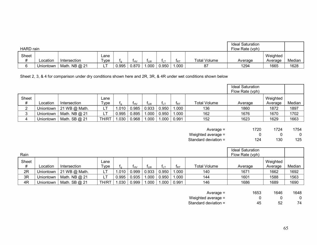
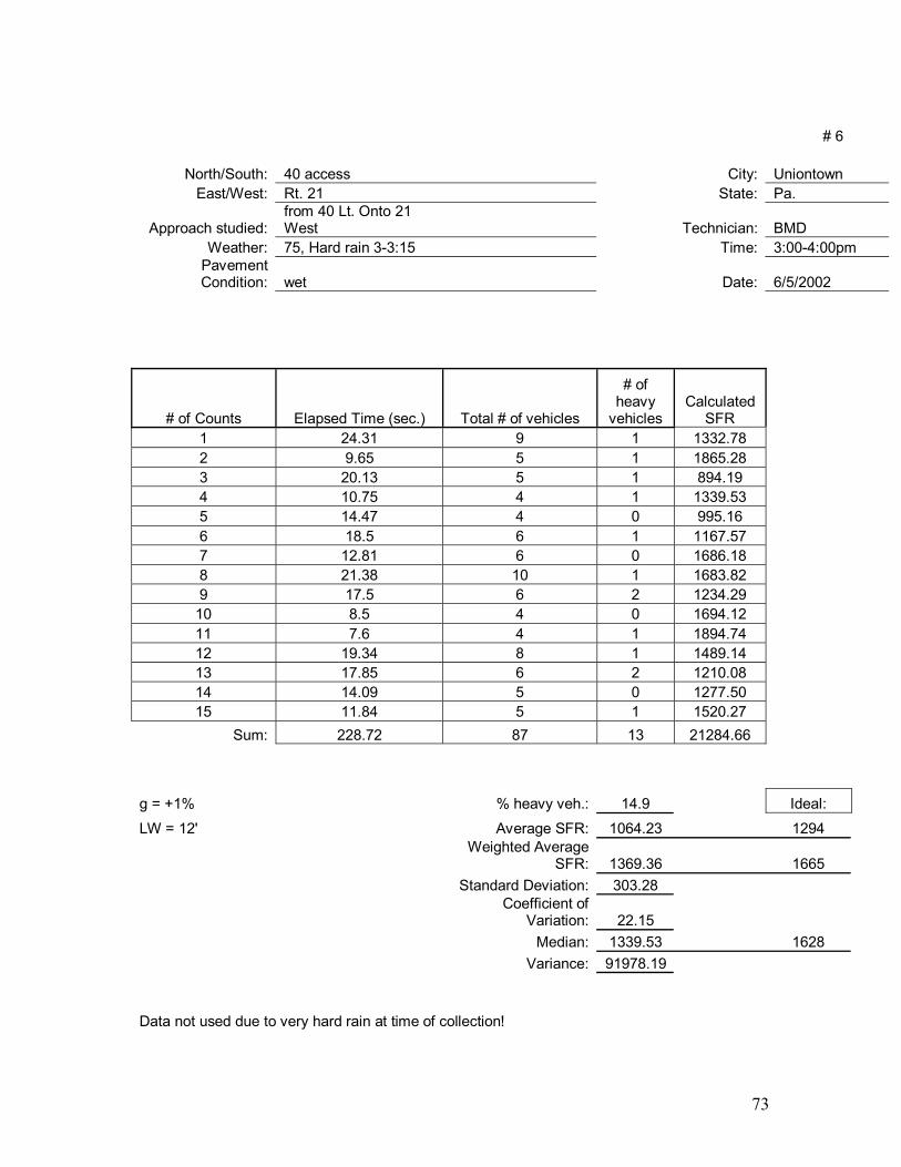
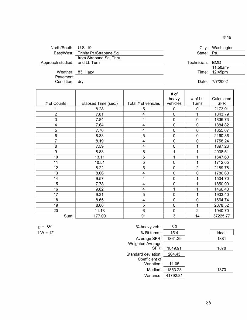
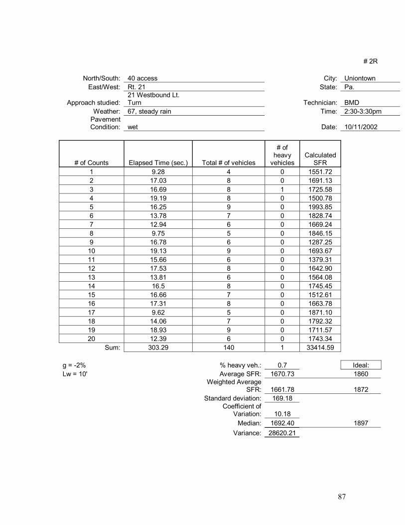
For the rain versus dry comparison, all data were collected in Uniontown at the

intersection of S.R. 0021 and S.R. 0119 / 0040 Ramps. The same approaches were

studied once under dry conditions and once while raining. The approaches studied were

as follows: S.R. 0021 Westbound left turn approach lane was designated as collection 2

under dry conditions and 2R under wet conditions, from S.R. 0119 / 0040 Ramps left turn

onto S.R. 0021 westbound approach lane was designated collection 3 under dry

conditions and 3R under wet conditions, and from southbound Matthew Drive

through/Right turn approach lane was designated collection 4 under dry conditions and

4R under wet conditions. All data collection sheets can be seen in the Appendix III. The

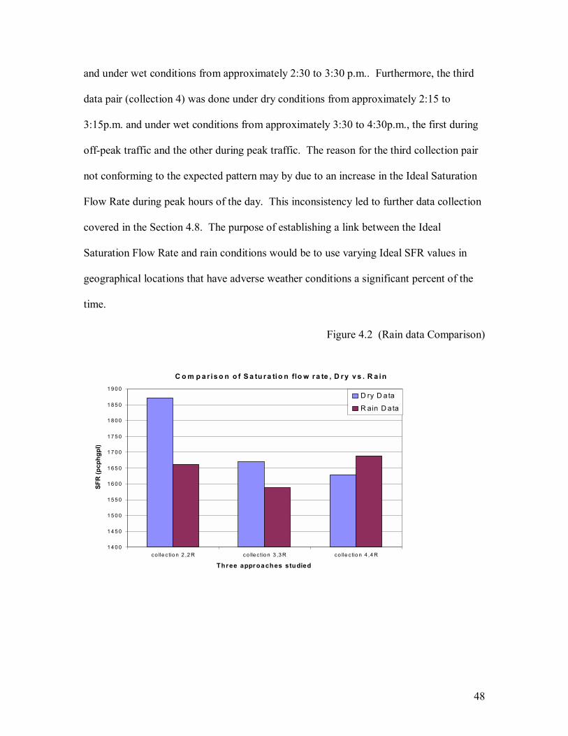
weighted averages for the Ideal Saturation Flow Rate are as follows, under dry

conditions, the SFR was 1717pcphgpl; under rain conditions, a value of 1646pcphgpl was

determined. While the weighted averages were approximately 70 pcphgpl higher for the

dry data, Figure 4.2 shows the data.

While the first two pairs show an obvious reduction in SFR under wet conditions,

as would be expected, the third does not. Data for the first two observation pairs were

collected at approximately the same time of day. The first two observations (collections

2 and 3) were both done under dry conditions both from approximately 1:15 to 2:15p.m.

48

and under wet conditions from approximately 2:30 to 3:30 p.m.. Furthermore, the third

data pair (collection 4) was done under dry conditions from approximately 2:15 to

3:15p.m. and under wet conditions from approximately 3:30 to 4:30p.m., the first during

off-peak traffic and the other during peak traffic. The reason for the third collection pair

not conforming to the expected pattern may by due to an increase in the Ideal Saturation

Flow Rate during peak hours of the day. This inconsistency led to further data collection

covered in the Section 4.8. The purpose of establishing a link between the Ideal

Saturation Flow Rate and rain conditions would be to use varying Ideal SFR values in

geographical locations that have adverse weather conditions a significant percent of the

time.

Figure 4.2 (Rain data Comparison)

C o m p a r is o n o f S a tu ra tio n flo w ra te , D ry v s . R a in

1 4 0 0

1 4 5 0

1 5 0 0

1 5 5 0

1 6 0 0

1 6 5 0

1 7 0 0

1 7 5 0

1 8 0 0

1 8 5 0

1 9 0 0

co lle c tio n 2 ,2 R co lle c t io n 3 ,3 R co lle c tio n 4 ,4 R

Three approaches studied

SFR

(pcp

hgpl

)

D ry D ata

R ain D ata

49

4.8 Ideal Saturation Flow Rate by Time of day

Due to the findings in Section 4.7, additional data were collected at one intersection to

check for variation in the Ideal Saturation Flow Rate from hour-to-hour throughout the

day. The intersection of S.R. 0119 / S.R. 0040 Ramps and S.R. 0021 in Uniontown was

studied continuously for five hours; results are shown in Figure 4.3. This is the same

intersection studied in the adverse weather condition data collection. For a continuous

five-hour period, data were collected for the traffic lane from S.R. 0119 / S.R. 0040

Ramps left-turn onto S.R. 0021. As seen in Figure 4.3, the one-hour collection periods

were used to determine a single ideal saturation flow rate shown on the figure at the end

of the one-hour period. At 12:00 the ideal saturation flow rate is at approximately

1790pcphgpl. From that time to 2:45pm the ideal saturation flow rate steadily decreases

to 1731pcphgpl. At that point, the ideal saturation flow rate begins to increase until 4:30

where it peaks at approximately 1910pcphgpl.

These findings would be useful for more technologically advanced signal controllers

offering the ability to vary signal timings over the course of the day.

50

Figure 4.3 (Time of Day Comparison)

4.9 Conclusions and Recommendations

In conclusion, the primary objective of this study was to determine if the District-wide

use of a 1800pcphgpl ideal saturation flow rate was warranted vs. the Highway Capacity

Manual�s recommended value of 1900pcphgpl. A quick glance at the results shows that

shows the weighted Ideal Saturation Flow Rate over the four-county region making up

PENNDOT District 12 was 1701pcphgpl, 100pcphgpl less than the ideal saturation flow

rate used by the district and 200pcphgpl less than the recommended value from the HCM.

It is evident from the later sections of the study that it would not be accurate to rely on

the above-mentioned information alone. Due to the time of day study, final adjustments

had to be made to the findings increasing the overall average in District 12-0 about

Variation in SFR vs. Time of day(Uniontown S.R. 0040 Ramp left-turn onto S.R. 0021)

1700

1750

1800

1850

1900

1950

1200 1300 1400 1500 1600 1700 1800

Time of day (military)

SFR

(pcp

hgpl

)

51

100pcphgpl and bringing the district-wide ideal saturation flow rate to 1801pcphgpl. If

PENNDOT District 12-0 is to use one ideal saturation flow rate district wide, the current

value of 1800pcphgpl is appropriate. In addition, the correction factors associated with

the HCM were tested. While the factors for lane type, grade, and heavy vehicle proved to

be adequate, the findings for the lane width correction factor were uncertain. Due to the

relationship between the Ideal Saturation Flow Rate and the correction factors, the impact

that the lane width factor could have on the study as a whole had to be accounted for.

Calculations were done to determine the impact of the lane width factor. It was

determined in this case the effects are minimal. When looked at on a district-wide level,

the factor can increase the Ideal SFR a maximum of approximately 15pcphgpl.

Furthermore, the only other section in this study that could affect the district- wide ideal

saturation flow rate would be the time-of-day study. Initial data collection was done

between the hours of 11:00 a.m. and 5:00 p.m. the majority falling between 12:00 p.m.

and 2:00 p.m., due to the findings in the adverse weather study, a secondary collection

was done to check for variation in the saturation flow rate throughout that time frame.

The findings were conclusive revealing an increase in the saturation flow rate of

approximately 100pcphgpl from off peak-to-peak travel times during the day. This

proves to be very important for accurately determining what the ideal saturation flow rate

for District 12 should be. As stated above, it was determined the saturation flow rate for

the district was 1701pcphgpl. Due to the majority of the data used in this finding being

collected at off-peak travel times, it would be necessary to adjust the SFR accordingly.

By doing so, the corrected District 12 ideal saturation flow rate would be approximately

1800pcpgpl, which is the value currently used by the District. Thus it is concluded due to

52

the reasonableness and stability of the results, that the methodology for estimating ideal

saturation flow rate is sound.

These findings would affect the comparisons done between counties and the individual

SFR�s for the counties. However increasing the SFR for the counties an equal amount

would not affect the relationship between them. The results for the comparison of

counties were also conclusive, showing a linear relationship between the saturation flow

rate and the geographical distance from the urban core. Additional research would need

to be done to more specifically determine the relationship and how it could be used to

adjust Ideal SFR for specific areas due to their geographical characteristics. A general

plan from the findings of this study alone would be to combine Fayette and Greene

counties with a proposed Ideal saturation flow rate of 1720pcphgpl, as well as

Washington and Westmoreland counties with a proposed ideal saturation flow rate of

1925pcphgpl. Note that both of the previous values recommended were adjusted due to

the findings in the time of day study.

The study for adverse weather conditions did show patterns but was overall inconclusive

due mainly to the change in ideal saturation flow rate between peak and off-peak periods.

The first two collection pairs revealed the weather conditions unfavorably affected the

SFR, but the last pair was skewed due to the collection under dry conditions during off-

peak period travel and under wet conditions during peak period travel. Further data

collection would need to be done while closely coordinating the collection times with

hours of the day to firmly prove or disprove the hypotheses.

While numerous tests were performed on various scenarios concerning the adjustment

factor for lane width, no conclusive evidence was found pinpointing the exact fault with

53

the factor. Extensive data collection that is beyond the scope of this research would need

to be done to arrive at a conclusion to the issue.

Chapter 5 � Conclusions

5.0 Conclusions

The primary objective of this study was to determine if the District-wide use of an

1800pcphgpl ideal saturation flow rate was warranted vs. the default value of 1900

pcphgpl recommended by the Highway Capacity Manual. Taking into consideration all

of the aforementioned findings, the current ideal saturation flow rate of 1800pcphgpl,

used by PENNDOT District 12-0, is appropriate if one value is used throughout the

district. From this study, due to there geographical characteristics it is evident that a

more localized approach should be used combining Fayette and Greene counties using an

ideal saturation flow rate of 1720pcphgpl and also combining Washington and

Westmoreland counties using an ideal saturation flow rate of 1925pcphgpl. In addition,

the adjustment factors associated with the HCM were tested, while the factors for lane

type, grade, and heavy vehicle proved to be adequate, the findings for the lane width

correction factor were uncertain. Due to the direct relation between the ideal saturation

flow rate and the correction factors, the impact the lane width factor could have on the

study as a whole had to be accounted for. Calculations were done to see specifically

what the impact the lane width factor could be and it was determined in this case the

effects are negligible. When looked at on a district-wide level, the factor can increase the

ideal saturation flow rate a maximum of approximately 15pcphgpl.

54

Moreover, the only other segment in this study that could affect the District-wide

ideal saturation flow rate would be the time-of-day study. Initial data collection was

done between the hours of 11:00 a.m. and 5:00 p.m., with the majority falling between

12:00 p.m. and 2:00 p.m.. Due to the findings in the adverse weather study, a secondary

collection was done to check for inconsistency in the ideal saturation flow rate

throughout that time frame. The findings were conclusive, revealing an increase in the

ideal saturation flow rate of approximately 100pcphgpl from off-peak to peak travel times

during the day. This proves to be crucial for determining what the ideal saturation flow

rate for District 12 should be. As stated above, it was determined the ideal saturation

flow rate for the District was 1701pcphgpl. However, due to the majority of the data

used in this finding being collected at off peak travel times it would be necessary to

adjust the SFR accordingly. By doing so, the corrected District 12 ideal saturation flow

rate would be approximately 1800pcphgpl, which is the value currently used by the

district at this time. Therefore it is concluded based on reasonableness and stability of the

results that the methodology for estimating the ideal saturation flow rate appears to be a

sound one.

These findings would affect the comparisons done between counties and the individual

SFR�s for the counties also. Conversely, increasing the SFR for all counties by an equal

amount would not influence the relationship between them. The results for the

comparison of counties were also conclusive, showing a linear relationship between the

saturation flow rate and the population density. Additional research would need to be

done to establish a relationship and how that relationship could be used to adjust ideal

saturation flow rate for specific areas based their geographical location.

55

The study for adverse weather conditions did show patterns that supported the hypothesis

of a reduced ideal saturation flow rate during rain events, but was overall inconclusive

due mainly to the change in ideal saturation flow rate over the course of a day. The first

two collection pairs proved the rainy weather conditions unfavorably affected the ideal

saturation flow rate, but the last pair was skewed due to the collection under dry

conditions during off-peak travel and under wet conditions during peak travel. Further

data collection would need to be done while closely coordinating the collection times

with the peak travel times to decisively prove or disprove the theory.

While numerous tests were performed on an assortment of scenarios concerning the

correction factor for lane width no conclusive evidence was found pinpointing the exact

trouble with the factor. Additional research that is beyond the scope of this project would

be needed to adequately represent all variations of the factor including lanes less than,

equal to, and greater than the ideal lane width of 12 feet.

5.1 Limitations of the Research and Recommendations for Further

Research

Upon completion of the project, a few limitations of the research should be identified.

First, a larger data set allows for more in-depth and conclusive data reduction to be

performed as well as addressing all areas to have a sufficient data set (i.e. lane width).

By doing so it will prevent unrelated factors from having an effect on the data set,

specific attention should be given making sure all data collection is done noting all

exterior factors (i.e. time of day and weather).

Some ideas for additional research would be to perform detailed time specific data

collection, which could be analyzed for determining varying ideal saturation flow rates

56

over the entire length of a day. Also, due to the problem encountered with the lane width

correction factor, extensive collection should be done to examine the validity of the

numbers used for the non-ideal lane widths.

57

References

6.0 References

Garber, Nicholas J. and Hoel, Lester A. Traffic and Highway Engineering

Second Edition. Brooks/Cole Publishing Company, 1999. 399-415, 460-469.

Lum, Harry S. �Statistical Shortcomings in Traffic Studies.� Public Roads Vol. 54, No. 4

(1991): 283-287

McMahon, Joseph W., Krane, John P., Federico, Albert P. �Saturation Flow Rates by

Facility Type.� ITE Journal January (1997): 46-50

NAVTEQ Inc. �Geographical Map� NAVTEQ Inc. 2003/Yahoo Inc. 2004 (10 March

2004) http://www.maps.yahoo.com/

Transportation Research Board National Research Council. Highway Capacity Manual

2000. Washington D.C.: TRB 2000. 16-9 to 16-18, 16-158 to16-160

Walpole, Ronald E., Myers, Raymond H., Myers, Sharon L. Probability and Statistics for

Engineers and Scientists Sixth Edition. Prentice Hall, Inc. 1998. 234-235, 461-

463

58

Appendix I

(Correction Factor Default Values)

59

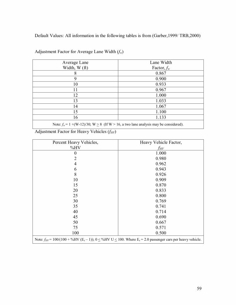
Default Values: All information in the following tables is from (Garber,1999/ TRB,2000) Adjustment Factor for Average Lane Width (fw)

Average Lane Width, W (ft)

Lane Width Factor, fw

8 0.867 9 0.900 10 0.933 11 0.967 12 1.000 13 1.033 14 1.067 15 1.100 16 1.133

Note: fw = 1 +(W-12)/30; W > 8 (If W > 16, a two lane analysis may be considered).

Adjustment Factor for Heavy Vehicles (fHV)

Percent Heavy Vehicles, %HV

Heavy Vehicle Factor, fHV

0 2 4 6 8 10 15 20 25 30 35 40 45 50 75

100

1.000 0.980 0.962 0.943 0.926 0.909 0.870 0.833 0.800 0.769 0.741 0.714 0.690 0.667 0.571 0.500

Note: fHV = 100/(100 + %HV (Er � 1)); 0 < %HV U < 100. Where Er = 2.0 passenger cars per heavy vehicle.

60

Adjustment Factor for Grade (fg)

Grade, %G Type Percent Grade Factor, fg

Downhill

Level Uphill

-6 or less -4 -2 0

+2 +4 +6 +8

+10 or more

1.030 1.020 1.010 1.000 0.990 0.980 0.970 0.960 0.950

Note: fg = 1- (%G)/200; -6 < %G < +10. Adjustment Factor for Parking (fp)

No. of Parking Maneuvers per Hour, Nm No. of

Lanes in Lane

Group, N No

Parking 0 10 20 30 40a 1 2 3a

1.000 1.000 1.000

0.900 0.950 0.967

0.850 0.925 0.950

0.800 0.900 0.933

0.750 0.875 0.917

0.700 0.850 0.900

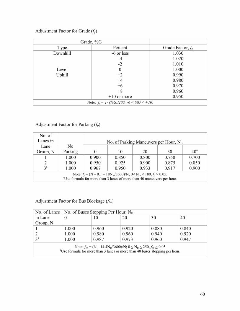
Note: fp = (N � 0.1 � 18Nm/3600)/N; 0< Nm < 180, fp > 0.05. aUse formula for more than 3 lanes of more than 40 maneuvers per hour.

Adjustment Factor for Bus Blockage (fbb)

No. of Buses Stopping Per Hour, NB No. of Lanes in Lane Group, N

0 10 20 30 40

1 2 3a

1.000 1.000 1.000

0.960 0.980 0.987

0.920 0.960 0.973

0.880 0.940 0.960

0.840 0.920 0.947

Note: fbb = (N � 14.4NB/3600)/N; 0 < NB < 250, fbb > 0.05 aUse formula for more than 3 lanes or more than 40 buses stopping per hour.

61

Default lane utilization factors (fLu)

Lane Group Movements

No. of Lanes In Lane Group

Percent of Traffic in Most Heavily Traveled Lane

Lane Utilization Factor (fLu)

1 100.0 1.00 2 3a

52.5 36.7

0.95 0.91

1 2a

100.0 51.5

1.00 0.97

Through or shared

Exclusive left turn

Exclusive right turn 1

2a 100.0 56.5

1.00 0.88

aIf lane group has more lanes than number shown in this table, it is recommended that surveys be made or the largest fLu-factor shown for that type of lane group be used

Adjustment Factor for Left Turns (fLT)

Lane Type (Protected Phasing) Formula Exclusive Lane fLT = 0.95

Shared Lane fLT = 1/(1.0 + 0.05PLT) Note: PLT = proportion of left turns in lane group.

Adjustment Factor for Right Turns (fRT)

Lane Type Formula Exclusive Lane fRT = 0.85

Shared Lane fRT = 1.0 � (0.15) PRT Single Lane fRT = 1.0 � (0.135) PRT

Note: PRT = proportion of right turns in lane group, fRT > 0.050

62

Adjustment Factor for Pedestrian-bicycle blockage (fLpb), and (fRpb)

Adjustment Direction Formula Left Adjustment fLpb = 1.0 � PLT(1 � Apbt)(1 � PLTA)

Right Adjustment fRpb = 1.0 � PRT(1 � Apbt)(1 � PRTA) Notes: PLT = proportion of left turns in lane group Apbt = permitted phase adjustment

PLTA = proportion of left turn protected green over total left turn green

PRT = proportion of right turns in lane group

PRTA = proportion of right turn protected green over total right turn green

63

Appendix II

(Data reduction Summary Sheets)

64

All initial data*

Ideal Saturation Flow Rate (vph)

Sheet # Location Intersection

Lane Type fg fHV fLW fLT fRT Total Volume Average

Weighted Average Median

1 Uniontown 21 EB @ Brew. TH/RT 1.015 0.906 0.967 1.000 0.992 213 1741 1721 1729 2 Uniontown 21 WB @ Math. LT 1.010 0.985 0.933 0.950 1.000 136 1860 1872 1897 3 Uniontown Math. NB @ 21 LT 0.995 0.895 1.000 0.950 1.000 162 1676 1670 1702 4 Uniontown Math. SB @ 21 TH/RT 1.030 0.968 1.000 1.000 0.991 152 1623 1629 1663 5 Uniontown Math. NB @ 21 TH 0.995 0.985 1.000 1.000 1.000 130 1636 1626 1645 7 Uniontown 21 WB @ McD's TH/RT 1.000 0.961 0.967 1.000 0.955 119 1721 1707 1684 8 Uniontown 21 WB @ McD's TH/RT 1.020 0.980 1.000 1.000 0.972 100 1478 1454 1526 9 Connellsville 119 NB @ Sheets TH/LT 1.000 0.950 1.000 0.989 1.000 132 1610 1589 1612

10 Connellsville 119 SB @ Wendys TH/LT 1.000 0.963 1.067 0.995 1.000 156 1593 1567 1596

11 Greensburg 119 NB @ ramps AB LT 0.995 0.955 0.967 0.950 1.000 85 1814 1799 1828

12 Greensburg 119 NB @ ramps CD LT 1.000 0.932 0.950 0.950 1.000 96 1829 1776 1915

13 Greensburg 119 SB @ ramps AB TH 1.005 0.964 0.950 1.000 1.000 82 1818 1807 1824

14 Waynesburg 21 EB @ McD's TH 1.005 0.987 1.067 1.000 1.000 93 1539 1524 1536 15 Waynesburg 19 SB @ 21 LT 0.985 0.989 1.000 0.950 1.000 87 1667 1651 1655 16 Washington Trin.Pt. @ 19 LT 1.030 1.000 1.000 0.950 1.000 83 1742 1728 1709 17 Washington 19 NB @ Trin. Pt. LT 1.030 1.000 0.967 0.950 1.000 83 2034 2024 2036 18 Washington 19 SB @ Trin. Pt. TH 0.965 0.990 0.967 1.000 1.000 98 1833 1814 1815 19 Washington Stra.Sq. @ 19 TH/LT 1.030 0.968 1.000 0.992 1.000 91 1881 1870 1873

Average = 1728 1713 1736 Weighted average = 0 0 0 Standard deviation = 139 141 140 * sheet number 6 excluded due to collection during hard rain.

65

HARD rain Ideal Saturation Flow Rate (vph)

Sheet # Location Intersection

Lane Type fg fHV fLW fLT fRT Total Volume Average

Weighted Average Median

6 Uniontown Math. NB @ 21 LT 0.995 0.870 1.000 0.950 1.000 87 1294 1665 1628 Sheet 2, 3, & 4 for comparison under dry conditions shown here and 2R, 3R, & 4R under wet conditions shown below

Ideal Saturation Flow Rate (vph)

Sheet # Location Intersection

Lane Type fg fHV fLW fLT fRT Total Volume Average

Weighted Average Median

2 Uniontown 21 WB @ Math. LT 1.010 0.985 0.933 0.950 1.000 136 1860 1872 1897 3 Uniontown Math. NB @ 21 LT 0.995 0.895 1.000 0.950 1.000 162 1676 1670 1702 4 Uniontown Math. SB @ 21 TH/RT 1.030 0.968 1.000 1.000 0.991 152 1623 1629 1663

Average = 1720 1724 1754 Weighted average = 0 0 0 Standard deviation = 124 130 125

Rain Ideal Saturation Flow Rate (vph)

Sheet # Location Intersection

Lane Type fg fHV fLW fLT fRT Total Volume Average

Weighted Average Median

2R Uniontown 21 WB @ Math. LT 1.010 0.999 0.933 0.950 1.000 140 1671 1662 1692 3R Uniontown Math. NB @ 21 LT 0.995 0.935 1.000 0.950 1.000 144 1601 1588 1563 4R Uniontown Math. SB @ 21 TH/RT 1.030 0.999 1.000 1.000 0.991 146 1686 1689 1690

Average = 1653 1646 1648 Weighted average = 0 0 0 Standard deviation = 45 52 74

66

Sheets 3-12 to 3-4 are of collections of the same intersection for a continuous five hour period 12:00 to 4:00 p.m.

Ideal Saturation Flow Rate (vph)

Sheet # Location Intersection Lane Type fg fHV fLW fLT fRT Total Volume Average

Weighted Average Median

3-12 Uniontown Math. NB @ 21 LT 0.995 0.941 1.000 0.950 1.000 96 1814 1791 1812 3-1 Uniontown Math. NB @ 22 LT 0.995 0.927 1.000 0.950 1.000 101 1755 1749 1727 3-2 Uniontown Math. NB @ 23 LT 0.995 0.924 1.000 0.950 1.000 97 1744 1731 1739 3-3 Uniontown Math. NB @ 24 LT 0.995 0.923 1.000 0.950 1.000 141 1898 1910 1938 3-4 Uniontown Math. NB @ 25 LT 0.995 0.920 1.000 0.950 1.000 138 1895 1895 1923

Average = 1821 1815 1828

Weighted average

= 0 0 0

Standard deviation

= 74 83 99

67

Appendix III

(Field collection/Data reduction sheets)

68

# 1

North/South: Brewer City: Uniontown East/West: Rt. 21 State: Pa.

Approach studied: 21 Eastbound St / Rt thru Technician: BMD

Weather: 82, clear Time: 12:07-1:10pm Pavement Condition: dry Date: 5/29/2002

# of Counts Elapsed Time (sec.) Total # of vehicles

# of heavy

vehicles # of Rt. Turns

Calculated SFR

1 16.28 8 0 1 1769.04 2 35.25 16 1 1 1634.04 3 22.69 9 2 0 1427.94 4 26.01 10 2 2 1384.08 5 30.22 10 2 2 1191.26 6 27.15 8 2 0 1060.77 7 23.85 13 0 0 1962.26 8 24.25 11 0 0 1632.99 9 21.22 9 0 0 1526.86

10 25.03 12 1 1 1725.93 11 29.16 13 2 0 1604.94 12 17.02 8 0 1 1692.13 13 25.38 10 2 1 1418.44 14 21.94 10 0 2 1640.84 15 26.75 11 1 1 1480.37 16 28.69 10 2 1 1254.79 17 28.68 12 2 0 1506.28 18 29.15 12 2 0 1481.99 19 17.91 9 0 0 1809.05 20 28.35 12 1 0 1523.81

Sum: 504.98 213 22 13 30727.82

g = -3% % heavy veh.: 10.3 Lw = 11' % Rt turns.: 6.1 Ideal:

Average SFR: 1536.39 1741

Weighted Average

SFR: 1518.48 1721 Standard deviation: 215.85

Coefficient of

Variation: 14.21 Median: 1525.34 1729 Variance: 46591.33

69

# 2

North/South: 40 access City: Uniontown East/West: Rt. 21 State: Pa.

Approach studied: 21 Westbound Lt. Turn Technician: BMD

Weather: 82, clear Time: 1:15-2:15pm Pavement Condition: dry Date: 5/29/2002

# of Counts Elapsed Time (sec.) Total # of vehicles

# of heavy

vehicles Calculated

SFR 1 11.12 4 0 1294.96 2 10.41 5 0 1729.11 3 14.53 6 0 1486.58 4 23.22 10 0 1550.39 5 10 5 0 1800.00 6 8.43 4 0 1708.19 7 16.59 8 0 1735.99 8 18.46 10 0 1950.16 9 10.5 5 0 1714.29

10 19.44 9 0 1666.67 11 14.5 7 0 1737.93 12 13.38 6 0 1614.35 13 23.56 11 1 1680.81 14 25.96 13 0 1802.77 15 19.82 9 0 1634.71 16 11 5 0 1636.36 17 10.38 4 0 1387.28 18 9.84 5 0 1829.27 19 11.4 5 0 1578.95 20 13.96 5 1 1289.40

Sum: 296.5 136 2 32828.17 g = -2% % heavy veh.: 1.5 Ideal: Lw = 10' Average SFR: 1641.41 1860

Weighted Average

SFR: 1651.26 1872 Standard deviation: 172.47

Coefficient of

Variation: 10.44 Median: 1673.74 1897 Variance: 29747.31

70

# 3

North/South: 40 access City: Uniontown East/West: Rt. 21 State: Pa.

Approach studied: from 40 Lt turn Technician: BMD

Weather: 82, clear Time: 1:15-2:25pm Pavement Condition: dry Date: 5/29/2002

# of Counts Elapsed

Time (sec.) Total # of vehicles

# of heavy

vehicles Calculated

SFR 1 19.87 8 2 1449.42 2 21.44 8 2 1343.28 3 16.82 6 1 1284.19 4 37.37 14 2 1348.68 5 22.15 6 2 975.17 6 17.68 8 0 1628.96 7 19.12 6 0 1129.71 8 19.2 8 0 1500.00 9 29.25 13 1 1600.00

10 10.73 5 0 1677.54 11 14.69 5 1 1225.32 12 15.25 6 0 1416.39 13 9.81 4 0 1467.89 14 10.06 4 0 1431.41 15 28.38 13 0 1649.05 16 29.12 14 1 1730.77 17 21.44 9 2 1511.19 18 25.69 9 2 1261.19 19 27.53 8 3 1046.13 20 17 8 0 1694.12

Sum: 412.6 162 19 28370.41 g = +1% % heavy veh.: 11.7 Ideal: Lw = 12' Average SFR: 1418.52 1676

Weighted Average

SFR: 1413.48 1670 Standard deviation: 217.52

Coefficient of

Variation: 15.39 Median: 1440.42 1702 Variance: 47316.11

71

# 4

North/South: 40 access City: Uniontown East/West: Rt. 21 State: Pa.

Approach studied:

from Walmart towards 40 St. / Rt. Technician: BMD

Weather: 82, clear Time: 2:15-3:20pm Pavement Condition: dry Date: 5/29/2002

# of Counts Elapsed Time

(sec.) Total # of vehicles # of heavy vehicles

# of Rt. Turns

Calculated SFR

1 13.63 8 1 0 2112.99 2 8.5 4 0 0 1694.12

3 21.41 10 0 1 1681.46 4 16.9 8 0 0 1704.14 5 12.88 4 1 0 1118.01 6 23.72 12 0 1 1821.25 7 22.44 10 0 0 1604.28 8 18.25 8 0 0 1578.08 9 20.57 9 0 1 1575.11

10 21.35 11 0 0 1854.80 11 13.25 6 0 2 1630.19 12 16.31 7 0 0 1545.06 13 18.81 9 0 2 1722.49 14 14.09 7 1 0 1788.50 15 13.41 4 1 0 1073.83 16 18.03 5 1 1 998.34 17 17.38 8 0 0 1657.08 18 20.44 9 0 2 1585.13 19 12.97 7 0 0 1942.95 20 15.53 6 0 0 1390.86

Sum: 339.87 152 5 10 32078.65 g = -7.7% % heavy veh.: 3.3 Lw = 12' % Rt turns.: 6.6 Ideal: Average SFR: 1603.93 1623

Weighted Average

SFR: 1610.03 1629 Standard deviation: 280.47

Coefficient of

Variation: 17.42 Median: 1643.63 1663

72

# 5

North/South: 40 access City: Uniontown East/West: Rt. 21 State: Pa.

Approach studied: from 40 St. thru. Technician: BMD

Weather: 82, clear Time: 3:36-4:45pm Pavement Condition: dry Date: 5/29/2002

# of Counts Elapsed Time

(sec.) Total # of vehicles

# of heavy

vehicles Calculated

SFR 1 7.75 4 0 1858.06 2 8.06 4 0 1786.60 3 9.78 4 0 1472.39 4 12.85 6 0 1680.93 5 10.62 5 0 1694.92 6 12.72 5 0 1415.09 7 19.1 9 0 1696.34 8 9.37 4 0 1536.82 9 18.17 8 0 1585.03

10 8.28 4 0 1739.13 11 20 9 1 1620.00 12 23.78 11 0 1665.26 13 18.69 7 0 1348.31 14 21.37 10 0 1684.60 15 8.81 4 0 1634.51 16 16.35 7 0 1541.28 17 18.04 8 1 1596.45 18 16.71 7 0 1508.08 19 12.95 5 0 1389.96 20 20.22 9 0 1602.37

Sum: 293.62 130 2 32056.16 g = -7.7% % heavy veh.: 1.5 Ideal: Lw = 12' Average SFR: 1602.81 1636

Weighted Average

SFR: 1593.90 1626 Standard deviation: 132.29

Coefficient of

Variation: 8.30 Median: 1611.19 1645 Variance: 17501.63

73

# 6

North/South: 40 access City: Uniontown East/West: Rt. 21 State: Pa.

Approach studied: from 40 Lt. Onto 21 West Technician: BMD

Weather: 75, Hard rain 3-3:15 Time: 3:00-4:00pm Pavement Condition: wet Date: 6/5/2002

# of Counts Elapsed Time (sec.) Total # of vehicles

# of heavy

vehicles Calculated

SFR 1 24.31 9 1 1332.78 2 9.65 5 1 1865.28 3 20.13 5 1 894.19 4 10.75 4 1 1339.53 5 14.47 4 0 995.16 6 18.5 6 1 1167.57 7 12.81 6 0 1686.18 8 21.38 10 1 1683.82 9 17.5 6 2 1234.29

10 8.5 4 0 1694.12 11 7.6 4 1 1894.74 12 19.34 8 1 1489.14 13 17.85 6 2 1210.08 14 14.09 5 0 1277.50 15 11.84 5 1 1520.27

Sum: 228.72 87 13 21284.66

g = +1% % heavy veh.: 14.9 Ideal: LW = 12' Average SFR: 1064.23 1294

Weighted Average

SFR: 1369.36 1665 Standard Deviation: 303.28

Coefficient of

Variation: 22.15 Median: 1339.53 1628 Variance: 91978.19 Data not used due to very hard rain at time of collection!

74

# 7

North/South: McDonalds access City: Uniontown East/West: Rt. 21 State: Pa.

Approach studied: 21 Westbound St. thru. Technician: BMD

Weather: 87, clear Time: 1:14-2:00pm Pavement Condition: dry Date: 6/5/2002

# of Counts Elapsed Time (sec.) Total # of vehicles

# of heavy

vehicles # of Rt. Turns

Calculated SFR

1 13.06 5 1 3 1378.25 2 11.72 5 0 3 1535.84 3 19.6 8 1 2 1469.39 4 17.25 7 0 3 1460.87 5 11.97 5 1 1 1503.76 6 17.12 7 0 4 1471.96 7 12.56 3 0 3 859.87 8 10.21 5 0 2 1762.98 9 23.03 10 0 3 1563.18

10 16.09 7 0 1 1566.19 11 13.47 7 0 1 1870.82 12 14.41 5 0 2 1249.13 13 17.01 7 0 3 1481.48 14 11.13 5 0 1 1617.25 15 7.82 4 0 1 1841.43 16 15.19 6 0 2 1421.99 17 15.53 6 1 3 1390.86 18 12.45 6 0 0 1734.94 19 9.93 4 0 1 1450.15 20 13.35 7 1 1 1887.64

Sum: 282.9 119 5 40 30517.99

g = +4% % heavy veh.: 4.2 LW = 11' % Rt turns.: 33.6 Ideal:

Average SFR: 1525.90 1721

Weighted Average

SFR: 1514.32 1707 Standard deviation: 235.12

Coefficient of

Variation: 15.53 Median: 1492.62 1684 Variance: 55279.41

75

# 8

North/South:

McDonalds access (work Parkway) City: Uniontown

East/West: Rt. 21 State: Pa.

Approach studied: 21 Eastbound Rt. / St. thru Technician: BMD

Weather: 87, clear Time: 2:00-2:50pm Pavement Condition: dry Date: 6/5/2002

# of Counts Elapsed Time

(sec.) Total # of vehicles

# of heavy vehicles

# of Rt. Turns Calculated SFR

1 12.44 4 1 2 1157.56

2 12.78 4 0 0 1126.76 3 9.5 4 0 2 1515.79 4 9.94 4 0 0 1448.69 5 12.97 5 0 2 1387.82 6 13.97 4 0 1 1030.78 7 9.25 4 0 2 1556.76 8 21.81 9 0 2 1485.56 9 18.47 6 1 2 1169.46 10 16.82 6 0 2 1284.19 11 20.22 8 0 1 1424.33 12 13.97 5 0 0 1288.48 13 8.59 4 0 2 1676.37 14 9.72 4 0 0 1481.48 15 8.52 4 0 0 1690.14 16 8.78 4 0 1 1640.09 17 8.81 4 0 1 1634.51 18 19.3 9 0 0 1678.76 19 9.4 4 0 1 1531.91 20 9.47 4 0 0 1520.59

Sum: 254.73 100 2 21 28730.02

g = -4% % heavy veh.: 2.0 LW = 12' % Rt turns.: 21.0 Ideal:

Average SFR: 1436.50 1478

Weighted

Average SFR: 1413.26 1454

Standard deviation: 200.00

Coefficient of

Variation: 14.15 Median: 1483.52 1526 Variance: 40000.56

76

# 9

North/South: 119 City: Connellsville East/West: 711 at corner of sheets State: Pa.

Approach studied: 119 N-bound Lt./St. (Lt. Lane) Technician: BMD

Weather: 86, Hazy Time: 2:15-3:10pm Pavement Condition: dry Date: 6/10/2002

# of Counts Elapsed Time (sec.) Total # of vehicles

# of heavy

vehicles # of Lt. Turns

Calculated SFR

1 13.53 6 0 2 1596.45 2 13.5 5 0 0 1333.33

3 19.58 10 0 1 1838.61 4 17.97 8 0 3 1602.67 5 15.72 5 1 1 1145.04 6 17.35 6 1 1 1244.96 7 10.13 5 0 1 1776.90 8 14.36 6 0 1 1504.18 9 19.56 7 1 1 1288.34

10 17.37 7 0 1 1450.78 11 16.23 7 0 2 1552.68 12 17.59 7 0 1 1432.63 13 9.44 4 0 0 1525.42 14 14.06 9 0 1 2304.41 15 13.53 7 0 1 1862.53 16 17.47 8 0 1 1648.54 17 16.44 8 0 10 1751.82 18 16.16 4 2 0 891.09 19 22.84 7 2 1 1103.33 20 15.38 6 0 1 1404.42

Sum: 318.21 132 7 30 30258.14

g = 0% % heavy veh.: 5.3 LW = 12' % Rt turns.: 22.7 Ideal:

Average SFR: 1512.91 1610

Weighted Average

SFR: 1493.35 1589 Standard deviation: 314.82

Coefficient of

Variation: 21.08 Median: 1514.80 1612 Variance: 99110.70

77

# 10

North/South: 119 City: Connellsville

East/West: 711 intersection at Wendys State: Pa.

Approach studied: Lt lane, 119 south St and Lt Technician: BMD

Weather: 89, Hazy Time: 3:30-4:21pm Pavement Condition: dry Date: 6/10/2002

# of Counts Elapsed Time (sec.) Total # of vehicles

# of heavy

vehicles # of Lt. Turns

Calculated SFR

1 15.53 7 0 0 1622.67 2 15.18 7 1 2 1660.08 3 18.94 9 1 2 1710.67 4 15.59 6 0 1 1385.50 5 29.47 10 2 4 1221.58 6 15.5 7 0 0 1625.81 7 15.03 7 0 0 1676.65 8 12.81 8 0 0 2248.24 9 16.59 5 1 1 1084.99

10 14.6 8 0 0 1972.60 11 18.65 8 0 1 1544.24 12 16.19 9 0 0 2001.24 13 16.24 6 0 0 1330.05 14 20.72 9 0 2 1563.71 15 17.06 8 0 2 1688.16 16 18.22 8 0 1 1580.68 17 17.39 7 1 0 1449.11 18 11.88 6 0 0 1818.18 19 20.66 10 0 0 1742.50 20 24.21 11 0 1 1635.69

Sum: 350.46 156 6 17 32562.33

g = 0% % heavy veh.: 3.8 LW = 15' % Rt turns.: 10.9 Ideal:

Average SFR: 1628.12 1593

Weighted Average

SFR: 1602.47 1567 Standard deviation: 267.44

Coefficient of

Variation: 16.69 Median: 1630.75 1596 Variance: 71525.39

78

# 11

North/South: 119 City: Greensburg East/West: 30 State: Pa.

Approach studied: 119 North, Lt turn onto 30 West Technician: BMD

Weather: 82, Hazy Time: 2:20-3:10pm Pavement Condition: dry Date: 6/12/2002

# of Counts Elapsed Time (sec.) Total # of vehicles

# of heavy

vehicles Calculated

SFR 1 10.53 4 1 1367.52 2 8.93 4 0 1612.54 3 8.18 4 0 1760.39 4 9.45 4 0 1523.81 5 9.63 4 0 1495.33 6 8.69 4 0 1657.08 7 11.96 4 1 1204.01 8 9.85 4 0 1461.93 9 10.22 5 0 1761.25

10 10.49 4 1 1372.74 11 7.97 4 0 1806.78 12 10.28 5 0 1750.97 13 9.25 4 0 1556.76 14 10.39 4 1 1385.95 15 14.22 6 0 1518.99 16 8.87 4 0 1623.45 17 8.34 4 0 1726.62 18 9.12 4 0 1578.95 19 8.37 4 0 1720.43 20 10.11 5 0 1780.42

Sum: 194.85 85 4 31665.90

g = +1.1% % heavy veh.: 4.7 Ideal: LW = 11' Average SFR: 1583.30 1814

Weighted Average

SFR: 1570.44 1799 Standard deviation: 167.30

Coefficient of

Variation: 10.65 Median: 1595.74 1828 Variance: 27987.69

79

# 12

North/South: 119 City: Greensburg East/West: 30 State: Pa.

Approach studied: 119 North, Rt onto 30 east Technician: BMD

Weather: 80, Hazy Time: 1:30-2:10pm Pavement Condition: dry Date: 6/12/2002

# of Counts Elapsed Time

(sec.) Total # of vehicles # of heavy vehicles

Calculated SFR

1 8.59 4 1 1676.37 2 14.22 4 1 1012.66 3 14.69 4 1 980.26 4 10.22 5 0 1761.25 5 8.94 4 0 1610.74 6 10.4 5 1 1730.77 7 10.41 4 0 1383.29 8 12.84 6 0 1682.24 9 11.09 6 0 1947.70

10 16.35 5 1 1100.92 11 12.38 4 0 1163.17 12 10.78 6 0 2003.71 13 8.47 5 0 2125.15 14 9.34 4 0 1541.76 15 13.21 4 1 1090.08 16 11.3 6 0 1911.50 17 9.56 5 0 1882.85 18 11 5 0 1636.36 19 12.69 5 1 1418.44 20 10.97 5 0 1640.84

Sum: 227.45 96 7 31300.05

g = +.3% % heavy veh.: 7.3 Ideal: LW = 11' Average SFR: 1565.00 1829

Weighted Average

SFR: 1519.45 1776 Standard deviation: 346.66

Coefficient of

Variation: 22.81 Median: 1638.60 1915 Variance: 120173.44

80

# 13

North/South: 119 City: Greensburg East/West: 30 State: Pa.

Approach studied: 119 south, St only at McD's Technician: BMD

Weather: 82, Hazy Time: 1:40-2:20pm Pavement Condition: dry Date: 6/12/2002

# of Counts Elapsed Time

(sec.) Total # of vehicles

# of heavy

vehicles Calculated

SFR 1 7.43 4 0 1938.09 2 10.37 5 0 1735.78 3 9.34 5 0 1927.19 4 7.78 4 0 1850.90 5 9.59 4 0 1501.56 6 8.4 4 0 1714.29 7 8.57 4 0 1680.28 8 8.31 4 0 1732.85 9 10.46 4 1 1376.67

10 8.6 4 0 1674.42 11 8.72 4 0 1651.38 12 8.63 4 0 1668.60 13 9.72 4 0 1481.48 14 8.35 4 0 1724.55 15 8.46 4 1 1702.13 16 7.88 4 0 1827.41 17 8.4 4 1 1714.29 18 9.56 4 0 1506.28 19 8.66 4 0 1662.82 20 7.25 4 0 1986.21

Sum: 174.48 82 3 34057.16

g = -.6% % heavy veh.: 3.7 Ideal: LW = 11' Average SFR: 1702.86 1818

Weighted Average

SFR: 1691.88 1807 Standard deviation: 156.84

Coefficient of

Variation: 9.27 Median: 1708.21 1824 Variance: 24600.33

81

# 14

North/South: McDonalds C42 B40/ LJ Silvers City: Wanesburg

East/West: Rt. 21 (East high Street) State: Pa. Approach studied: 21 East St. only Technician: BMD

Weather: 65, overcast Time: 6:50-8:10am Pavement Condition: dry Date: 6/4/2002

# of Counts Elapsed Time (sec.) Total # of vehicles

# of heavy

vehicles Calculated

SFR 1 7.9 4 0 1822.78 2 13.79 5 0 1305.29 3 11.44 5 0 1573.43 4 8.2 4 0 1756.10 5 10.35 5 0 1739.13 6 7.35 4 0 1959.18 7 10.56 4 0 1363.64 8 11.63 6 1 1857.27 9 10.29 4 0 1399.42

10 10.34 4 0 1392.65 11 9.82 4 0 1466.40 12 9.94 5 0 1810.87 13 13.63 6 0 1584.74 14 13.03 6 0 1657.71 15 8.79 4 0 1638.23 16 10.43 5 0 1725.79 17 12.28 5 0 1465.80 18 9.5 4 0 1515.79 19 11.75 5 0 1531.91 20 8.5 4 1 1694.12

Sum: 209.52 93 2 32260.23

g = -1% % heavy veh.: 2.2 Ideal: LW = 14' Average SFR: 1613.01 1539

Weighted Average

SFR: 1597.94 1524 Standard deviation: 182.61

Coefficient of

Variation: 11.43 Median: 1611.48 1536

82

# 15

North/South: Rt. 19 City: Wanesburg East/West: Rt. 21 State: Pa.

Approach studied: 19 south Lt. Turn to 21 East Technician: BMD

Weather: 75, overcast Time: 8:20-9:20am Pavement Condition: dry Date: 6/4/2002

# of Counts Elapsed Time (sec.) Total # of vehicles

# of heavy

vehicles Calculated

SFR 1 11.72 5 1 1535.84 2 9.63 4 0 1495.33 3 9.25 4 0 1556.76 4 11.47 5 0 1569.31 5 9.35 4 0 1540.11 6 7.5 4 0 1920.00 7 8.59 4 0 1676.37 8 9.9 4 0 1454.55 9 10.75 4 0 1339.53

10 11.82 5 0 1522.84 11 11.28 5 0 1595.74 12 11.13 6 0 1940.70 13 11.63 4 0 1238.18 14 8.25 4 0 1745.45 15 9.97 4 0 1444.33 16 11.18 4 0 1288.01 17 8.16 4 0 1764.71 18 12 4 0 1200.00 19 9.43 4 0 1527.04 20 12.03 5 0 1496.26

Sum: 205.04 87 1 30851.06

g = +3.4% % heavy veh.: 1.1 Ideal: LW = 12' Average SFR: 1542.55 1667

Weighted Average

SFR: 1527.507 1651 Standard deviation: 198.89

Coefficient of

Variation: 13.02 Median: 1531.44 1655 Variance: 39558.00

83

# 16

North/South: U.S. 19 City: Washington East/West: Trinity Pt/ Strabane Sq. State: Pa.

Approach studied: From Trinity Pt Lt turn only Technician: BMD

Weather: 85, Hazy Time: 1:00-1:45pm Pavement Condition: dry Date: 7/7/2002

# of Counts Elapsed Time (sec.) Total # of vehicles

# of heavy

vehicles Calculated

SFR 1 9.23 4 0 1560.13 2 10.15 4 0 1418.72 3 9.11 4 0 1580.68 4 9.47 4 0 1520.59 5 7.82 4 0 1841.43 6 8.13 4 0 1771.22 7 7.72 4 0 1865.28 8 9.11 4 0 1580.68 9 7 4 0 2057.14

10 8.01 4 0 1797.75 11 8.56 4 0 1682.24 12 9.75 5 0 1846.15 13 9.96 4 0 1445.78 14 8.25 4 0 1745.45 15 8.16 4 0 1764.71 16 11.13 5 0 1617.25 17 8.33 5 0 2160.86 18 8.66 4 0 1662.82 19 9.31 4 0 1546.72 20 8.84 4 0 1628.96

Sum: 176.7 83 0 34094.59

g = -8% % heavy veh.: 0.0 Ideal: LW = 12' Average SFR: 1704.73 1742

Weighted Average

SFR: 1691.00 1728 Standard deviation: 190.5835

Coefficient of

Variation: 11.27 Median: 1672.53 1709 Variance: 36322.07

84

# 17

North/South: U.S. 19 City: Washington

East/West: Trinity Pt/ Strabane Sq. State: Pa.

Approach studied: 19 North Lt turn only Technician: BMD

Weather: 83, Hazy Time:11:45am-12:30pm

Pavement Condition: dry Date: 7/7/2002

# of Counts Elapsed Time (sec.) Total # of vehicles

# of heavy

vehicles Calculated

SFR 1 8.85 5 0 2033.90 2 7.11 4 0 2025.32 3 7.01 4 0 2054.21 4 8.97 5 0 2006.69 5 7.88 4 0 1827.41 6 8.11 4 0 1775.59 7 8.95 5 0 2011.17 8 7.83 4 0 1839.08 9 7.35 4 0 1959.18

10 8.07 4 0 1784.39 11 7.19 4 0 2002.78 12 6.5 4 0 2215.38 13 6.72 4 0 2142.86 14 8.22 4 0 1751.82 15 8.31 4 0 1732.85 16 8.18 4 0 1760.39 17 6.5 4 0 2215.38 18 8.81 4 0 1634.51 19 7.91 4 0 1820.48 20 7.6 4 0 1894.74

Sum: 156.07 83 0 38488.13

g = -7.1% % heavy veh.: 0.0 Ideal: LW = 11' Average SFR: 1924.41 2034

Weighted Average

SFR: 1914.53 2024 Standard deviation: 166.27

Coefficient of

Variation: 8.68 Median: 1926.96 2036 Variance: 27645.87

85

# 18

North/South: U.S. 19 City: Washington

East/West: Trinity Pt./Strabane Sq. State: Pa.

Approach studied: 19 South, thru (Rt lane) Technician: BMD

Weather: 85, Hazy Time: 1:00-1:40pm Pavement Condition: dry Date: 7/7/2002

# of Counts Elapsed Time (sec.) Total # of vehicles

# of heavy

vehicles Calculated

SFR 1 11.18 5 0 1610.02 2 17.14 5 1 1050.18 3 9.11 4 0 1580.68 4 7.62 4 0 1889.76 5 10.38 5 0 1734.10 6 10.56 6 0 2045.45 7 8.69 4 0 1657.08 8 10.94 5 0 1645.34 9 12.19 7 0 2067.27

10 9.1 4 0 1582.42 11 12.63 5 0 1425.18 12 8.75 4 0 1645.71 13 8.5 4 0 1694.12 14 9.94 5 0 1810.87 15 12.64 6 0 1708.86 16 12.94 7 0 1947.45 17 8.24 4 0 1747.57 18 8.68 4 0 1658.99 19 10.33 5 0 1742.50 20 11.06 5 0 1627.49

Sum: 210.62 98 1 33871.03

g = +6.7% % heavy veh.: 1.0 Ideal: LW = 11' Average SFR: 1693.55 1833

Weighted Average

SFR: 1675.05 1814 Standard deviation: 219.68

Coefficient of

Variation: 13.11 Median: 1676.55 1815 Variance: 48260.42

86

# 19

North/South: U.S. 19 City: Washington East/West: Trinity Pt./Strabane Sq. State: Pa.

Approach studied: from Strabane Sq, Thru and Lt. Turn Technician: BMD

Weather: 83, Hazy Time:11:50am-12:45pm

Pavement Condition: dry Date: 7/7/2002

# of Counts Elapsed Time (sec.) Total # of vehicles

# of heavy

vehicles # of Lt. Turns

Calculated SFR

1 8.28 5 0 0 2173.91 2 7.81 4 0 1 1843.79 3 7.84 4 0 0 1836.73 4 7.64 4 0 0 1884.82 5 7.76 4 0 0 1855.67 6 8.33 5 0 0 2160.86 7 8.19 4 0 0 1758.24 8 7.59 4 0 1 1897.23 9 8.83 5 1 1 2038.51

10 13.11 6 1 1 1647.60 11 10.51 5 0 1 1712.65 12 8.22 5 0 2 2189.78 13 8.06 4 0 0 1786.60 14 9.57 4 0 1 1504.70 15 7.78 4 0 1 1850.90 16 9.82 4 1 1 1466.40 17 9.31 5 0 1 1933.40 18 8.65 4 0 0 1664.74 19 8.66 5 0 1 2078.52 20 11.13 6 0 2 1940.70

Sum: 177.09 91 3 14 37225.77

g = -8% % heavy veh.: 3.3 LW = 12' % Rt turns.: 15.4 Ideal:

Average SFR: 1861.29 1881

Weighted Average

SFR: 1849.91 1870 Standard deviation: 204.43

Coefficient of

Variation: 11.05 Median: 1853.28 1873 Variance: 41792.81

87

# 2R

North/South: 40 access City: Uniontown East/West: Rt. 21 State: Pa.

Approach studied: 21 Westbound Lt. Turn Technician: BMD

Weather: 67, steady rain Time: 2:30-3:30pm Pavement Condition: wet Date: 10/11/2002

# of Counts Elapsed Time (sec.) Total # of vehicles

# of heavy

vehicles Calculated

SFR 1 9.28 4 0 1551.72 2 17.03 8 0 1691.13 3 16.69 8 1 1725.58 4 19.19 8 0 1500.78 5 16.25 9 0 1993.85 6 13.78 7 0 1828.74 7 12.94 6 0 1669.24 8 9.75 5 0 1846.15 9 16.78 6 0 1287.25

10 19.13 9 0 1693.67 11 15.66 6 0 1379.31 12 17.53 8 0 1642.90 13 13.81 6 0 1564.08 14 16.5 8 0 1745.45 15 16.66 7 0 1512.61 16 17.31 8 0 1663.78 17 9.62 5 0 1871.10 18 14.06 7 0 1792.32 19 18.93 9 0 1711.57 20 12.39 6 0 1743.34

Sum: 303.29 140 1 33414.59 g = -2% % heavy veh.: 0.7 Ideal: Lw = 10' Average SFR: 1670.73 1860

Weighted Average

SFR: 1661.78 1872 Standard deviation: 169.18

Coefficient of

Variation: 10.18 Median: 1692.40 1897 Variance: 28620.21

88

# 3R

North/South: 40 access City: Uniontown East/West: Rt. 21 State: Pa.

Approach studied: from 40 Lt turn Technician: BMD

Weather: 67, steady rain Time: 2:30-3:20pm Pavement Condition: wet Date: 10/11/2002

# of Counts Elapsed

Time (sec.) Total # of vehicles

# of heavy

vehicles Calculated

SFR 1 8.69 4 0 1657.08 2 11.72 5 1 1535.84 3 16.07 6 2 1344.12 4 14.6 6 0 1479.45 5 23.85 9 1 1358.49 6 24.6 10 1 1463.41 7 12.03 7 0 2094.76 8 10.13 4 0 1421.52 9 12.63 5 1 1425.18

10 18.06 8 1 1594.68 11 20.88 10 1 1724.14 12 9.72 5 0 1851.85 13 19.84 10 1 1814.52 14 22.63 10 0 1590.81 15 16.5 8 0 1745.45 16 18.44 9 0 1757.05 17 19.09 8 0 1508.64 18 13.06 7 0 1929.56 19 19.03 8 1 1513.40 20 14.94 5 0 1204.82

Sum: 326.51 144 10 32014.77 g = +1% % heavy veh.: 6.9 Ideal: Lw = 12' Average SFR: 1600.74 1676

Weighted Average

SFR: 1587.70 1670 Standard deviation: 220.40

Coefficient of

Variation: 13.88 Median: 1563.32 1702 Variance: 48577.52

89

# 4R

North/South: 40 access City: Uniontown East/West: Rt. 21 State: Pa.

Approach studied: from Walmart towards 40 St. / Rt. Technician: BMD

Weather: 67, steady rain Time: 3:40-4:30pm Pavement Condition: wet Date: 10/11/2002

# of Counts Elapsed Time (sec.) Total # of vehicles

# of heavy

vehicles # of Rt. Turns

Calculated SFR

1 12.79 6 0 1 1688.82 2 12.16 6 0 0 1776.32 3 12.3 5 0 0 1463.41 4 13.29 6 0 1 1625.28 5 12.06 6 0 0 1791.04 6 11 6 0 0 1963.64 7 15.43 7 0 0 1633.18 8 13.69 5 1 1 1314.83 9 13.18 6 0 0 1638.85

10 14.28 7 0 0 1764.71 11 13.78 6 0 1 1567.49 12 17.63 9 0 0 1837.78 13 19.82 9 0 0 1634.71 14 18.37 10 0 0 1959.72 15 21.28 10 0 0 1691.73 16 18.75 9 0 0 1728.00 17 19 9 0 0 1705.26 18 16.13 8 0 0 1785.49 19 14.13 6 0 0 1528.66 20 22.19 10 0 0 1622.35

Sum: 311.26 146 1 4 33721.27 g = -7.7% % heavy veh.: 0.7 Lw = 12' % Rt turns.: 2.7 Ideal: Average SFR: 1686.06 1623

Weighted Average

SFR: 1688.62 1629 Standard deviation: 154.58

Coefficient of

Variation: 9.15 Median: 1690.27 1663 Variance: 23894.39

90

# 3-12

North/South: 40 access City: Uniontown East/West: Rt. 21 State: Pa.

Approach studied: from 40 Lt turn Technician: BMD

Weather: 52, cloudy Time: 12:00-1:00 Pavement Condition: dry Date: 10/23/2002

# of Counts Elapsed

Time (sec.) Total # of vehicles # of heavy vehicles

Calculated SFR

1 11.79 4 1 1221.37 2 11.97 5 0 1503.76 3 11.02 4 0 1306.72 4 9.38 4 1 1535.18 5 16.31 6 2 1324.34 6 8.06 4 0 1786.60 7 9.72 4 0 1481.48 8 8.56 4 0 1682.24 9 8.5 4 0 1694.12

10 10.05 5 0 1791.04 11 17.47 7 0 1442.47 12 10.66 5 1 1688.56 13 15.5 7 0 1625.81 14 15.63 6 1 1381.96 15 9.07 4 0 1587.65 16 10.73 5 0 1677.54 17 11.2 4 0 1285.71 18 14.13 6 0 1528.66 19 8.88 4 0 1621.62 20 9.41 4 0 1530.29

Sum: 228.04 96 6 30697.13 g = +1% % heavy veh.: 6.3 Ideal: Lw = 12' Average SFR: 1534.86 1814

Weighted Average

SFR: 1515.52 1791 Standard deviation: 167.20

Coefficient of

Variation: 11.03 Median: 1532.73 1812 Variance: 27955.79

91

# 3-1

North/South: 40 access City: Uniontown East/West: Rt. 21 State: Pa.

Approach studied: from 40 Lt turn Technician: BMD

Weather: 53, cloudy Time: 1:00-2:00 Pavement Condition: dry Date: 10/23/2002

# of Counts Elapsed

Time (sec.) Total # of vehicles

# of heavy

vehicles Calculated

SFR 1 10.2 4 0 1411.76 2 14.04 7 1 1794.87 3 11.33 5 0 1588.70 4 11.03 4 0 1305.53 5 10.83 4 1 1329.64 6 9.28 4 1 1551.72 7 18.03 9 0 1797.00 8 16.56 6 1 1304.35 9 9.03 4 1 1594.68

10 17.91 6 1 1206.03 11 16.73 6 0 1291.09 12 9.85 4 0 1461.93 13 8.88 4 0 1621.62 14 14.72 7 1 1711.96 15 9.18 4 0 1568.63 16 10 4 0 1440.00 17 11.16 4 0 1290.32 18 15.89 6 1 1359.35 19 11.21 5 0 1605.71 20 9.86 4 0 1460.45

Sum: 245.72 101 8 29695.35 g = +1% % heavy veh.: 7.9 Ideal: Lw = 12' Average SFR: 1484.77 1755

Weighted Average

SFR: 1479.73 1749 Standard deviation: 174.56

Coefficient of

Variation: 11.80 Median: 1461.19 1727 Variance: 30471.56

92

# 3-2

North/South: 40 access City: Uniontown East/West: Rt. 21 State: Pa.

Approach studied: from 40 Lt turn Technician: BMD

Weather: 53, cloudy Time: 2:00-3:00 Pavement Condition: dry Date: 10/23/2002

# of Counts Elapsed

Time (sec.) Total # of vehicles

# of heavy

vehicles Calculated

SFR 1 11.37 6 0 1899.74 2 9.19 4 1 1566.92 3 12.59 5 1 1429.71 4 10.04 4 0 1434.26 5 9.89 4 0 1456.02 6 10.69 4 0 1347.05 7 9.4 4 0 1531.91 8 17.28 6 2 1250.00 9 10.32 4 0 1395.35

10 14.53 6 0 1486.58 11 18.88 8 2 1525.42 12 14.19 6 0 1522.20 13 12.44 5 1 1446.95 14 10.06 4 0 1431.41 15 9.01 4 0 1598.22 16 9.48 4 0 1518.99 17 13.69 5 1 1314.83 18 9.38 4 0 1535.18 19 11.59 5 0 1553.06 20 14.44 5 0 1246.54

Sum: 238.46 97 8 29490.34 g = +1% % heavy veh.: 8.2 Ideal: Lw = 12' Average SFR: 1474.52 1744

Weighted Average

SFR: 1464.40 1731 Standard deviation: 141.75

Coefficient of

Variation: 9.68 Median: 1471.30 1739 Variance: 20093.27

93

# 3-3

North/South: 40 access City: Uniontown East/West: Rt. 21 State: Pa.

Approach studied: from 40 Lt turn Technician: BMD

Weather: 53, cloudy Time: 3:00-4:00 Pavement Condition: dry Date: 10/23/2002

# of Counts Elapsed

Time (sec.) Total # of vehicles

# of heavy

vehicles Calculated

SFR 1 17.07 8 0 1687.17 2 11.82 6 0 1827.41 3 17.4 8 0 1655.17 4 18.16 8 1 1585.90 5 11.12 4 2 1294.96 6 19.71 9 1 1643.84 7 11.63 5 1 1547.72 8 19.53 9 0 1658.99 9 16.81 8 0 1713.27

10 10.83 4 0 1329.64 11 10.92 5 0 1648.35 12 11 5 0 1636.36 13 14.56 6 1 1483.52 14 22.94 10 0 1569.31 15 17.86 9 0 1814.11 16 19.31 9 0 1677.89 17 17.65 8 2 1631.73 18 9.72 4 1 1481.48 19 19.74 8 1 1458.97 20 16.19 8 1 1778.88

Sum: 313.97 141 11 32124.66 g = +1% % heavy veh.: 7.8 Ideal: Lw = 12' Average SFR: 1606.23 1898

Weighted Average

SFR: 1616.71 1910 Standard deviation: 142.52

Coefficient of

Variation: 8.82 Median: 1640.10 1938 Variance: 20310.79

94

# 3-4

North/South: 40 access City: Uniontown East/West: Rt. 21 State: Pa.

Approach studied: from 40 Lt turn Technician: BMD

Weather: 55, cloudy Time: 4:00-5:00 Pavement Condition: dry Date: 10/23/2002

# of Counts Elapsed

Time (sec.) Total # of vehicles

# of heavy

vehicles Calculated

SFR 1 12.72 6 0 1698.11 2 18.19 7 1 1385.38 3 13.22 6 0 1633.89 4 12.44 6 0 1736.33 5 9.56 4 1 1506.28 6 18.84 7 2 1337.58 7 20.81 10 0 1729.94 8 9.57 4 0 1504.70 9 15.43 7 0 1633.18

10 14.78 7 1 1705.01 11 11.31 5 2 1591.51 12 17.59 8 0 1637.29 13 9.41 4 0 1530.29 14 22.21 10 0 1620.89 15 22.34 10 1 1611.46 16 19.06 8 1 1511.02 17 19.18 9 1 1689.26 18 13.97 7 0 1803.87 19 16.21 7 1 1554.60 20 13.06 6 1 1653.91

Sum: 309.9 138 12 32074.48 g = +1% % heavy veh.: 8.7 Ideal: Lw = 12' Average SFR: 1603.72 1895

Weighted Average

SFR: 1603.10 1895 Standard deviation: 117.02

Coefficient of

Variation: 7.30 Median: 1627.04 1923 Variance: 13694.37

95

Appendix IV

(ANOVA analysis output sheets)

96

Weighted Average SFR ANOVA analysis 1 2 3 4 1721 1799 1524 1728 1872 1776 1651 2024 1670 1807 1814 1629 1870 1626 1707 1454 1589 1567 ANOVA: Single Factor SUMMARY Groups Count Sum Average Variance Column 1 9 14835 1648.333 13499 Column 2 3 5382 1794 259 Column 3 2 3175 1587.5 8064.5 Column 4 4 7436 1859 15510.67 ANOVA

Source of Variation SS df MS F P-value F crit

Between Groups 174082 3 58027.17 4.980674 0.014773 3.343885 Within Groups 163107 14 11650.46 Total 337188 17 Samples are statistically different.

97

Unweighted Average SFR ANOVA analysis 1 2 3 4 1741 1814 1539 1742 1860 1829 1667 2034 1676 1818 1833 1623 1881 1636 1721 1478 1610 1593 ANOVA: Single Factor SUMMARY Groups Count Sum Average Variance Column 1 9 14938 1659.778 11574.44 Column 2 3 5461 1820.333 60.33333 Column 3 2 3206 1603 8192 Column 4 4 7490 1872.5 14915 ANOVA

Source of Variation SS df MS F P-value F crit

Between Groups 182231 3 60743.76 5.838612 0.008379 3.343885 Within Groups 145653 14 10403.8 Total 327885 17 Samples are statistically different.

98

Unweighted Average SFR ANOVA analysis 1 2 3 4 1741 1814 1539 1742 1860 1829 1667 2034 1676 1818 1833 1623 1881 1636 1721 1478 1610 1593 ANOVA: Single Factor SUMMARY Groups Count Sum Average Variance Column 1 9 14938 1659.778 11574.44 Column 2 3 5461 1820.333 60.33333 Column 3 2 3206 1603 8192 Column 4 4 7490 1872.5 14915 ANOVA

Source of Variation SS df MS F P-value F crit

Between Groups 182231 3 60743.76 5.838612 0.008379 3.343885 Within Groups 145653 14 10403.8 Total 327885 17 Samples are statistically different.

99

Median SFR ANOVA analysis

1 2 3 4 1729 1828 1536 1709 1897 1915 1655 2036 1702 1824 1815 1663 1873 1645 1684 1526 1612 1596 ANOVA: Single Factor SUMMARY Groups Count Sum Average Variance Column 1 9 15054 1672.667 10802 Column 2 3 5567 1855.667 2644.333 Column 3 2 3191 1595.5 7080.5 Column 4 4 7433 1858.25 18652.92 ANOVA

Source of Variation SS df MS F P-value F crit

Between Groups 178321 3 59440.19 5.377676 0.011301 3.343885 Within Groups 154744 14 11053.14 Total 333065 17 Samples are statistically different.

100

ANOVA analysis between Fayette and Greene counties using weighted SFR Fayette Greene 1721 1524 1872 1651 1670 1629 1626 1707 1454 1589 1567 ANOVA: Single Factor SUMMARY Groups Count Sum Average Variance Column 1 9 14835 1648.333 13499 Column 2 2 3175 1587.5 8064.5 ANOVA

Source of Variation SS df MS F P-value F crit

Between Groups 6055.68 1 6055.682 0.469609 0.51043 5.117357 Within Groups 116057 9 12895.17 Total 122112 10 Samples are not statistically different.

101

ANOVA analysis between Washington and Westmoreland counties using weighted SFR Washington Westmoreland 1728 1799 2024 1776 1814 1807 1870 ANOVA: Single Factor SUMMARY Groups Count Sum Average Variance Column 1 4 7436 1859 15510.67 Column 2 3 5382 1794 259 ANOVA

Source of Variation SS df MS F P-value F crit

Between Groups 7242.86 1 7242.857 0.769698 0.420459 6.607877 Within Groups 47050 5 9410 Total 54292.9 6 Samples are not statistically different.

102

Counties Fayette&Greene vs. Washington&Westmoreland Weighted SFR ANOVA analysis F&G W&W 1721 1728 1872 2024 1670 1814 1629 1870 1626 1799 1707 1776 1454 1807 1589 1567 1524 1651 ANOVA: Single Factor SUMMARY Groups Count Sum Average Variance Column 1 11 18010 1637.273 12211.22 Column 2 7 12818 1831.143 9048.81 ANOVA

Source of Variation SS df MS F P-value F crit

Between Groups 160783 1 160783 14.58307 0.001512 4.493998 Within Groups 176405 16 11025.31 Total 337188 17 Samples are statistically different.

103

Lane type, weighted SFR ANOVA analysis LT TH Shared 1 2 3 1872 1626 1721 1670 1807 1629 1799 1524 1707 1776 1814 1454 1651 1589 1728 1567 2024 1870 ANOVA: Single Factor SUMMARY Groups Count Sum Average Variance Column 1 7 12520 1788.571 16551.29 Column 2 4 6771 1692.75 20228.92 Column 3 7 11537 1648.143 17688.81 ANOVA

Source of Variation SS df MS F P-value F crit

Between Groups 71060.7 2 35530.34 2.002632 0.169485 3.682317 Within Groups 266127 15 17741.82 Total 337188 17 0.16>.05, hypothesis is correct, they are the same 2.003<3.682, hypothesis is correct, they are the same

104

ANOVA analysis to test grade factor using weighted SFR negative grade 0 grade positive grade 1721 1707 1670 1872 1589 1626 1629 1567 1799 1454 1776 1651 1807 1814 1524 1728 2024 1870 ANOVA: Single Factor SUMMARY Groups Count Sum Average Variance Column 1 9 15629 1736.556 32580.03 Column 2 4 6639 1659.75 9784.917 Column 3 5 8560 1712 7713.5 ANOVA Source of Variation SS df MS F P-value F crit Between Groups 16339 2 8169.514 0.381933 0.688992 3.682317 Within Groups 320849 15 21389.93 Total 337188 17 Samples are not statistically different.

105

ANOVA analysis to test lane width factor using weighted SFR

< 12' lanes 12' lanes

> 12' lanes

1721 1670 1567 1872 1629 1524 1707 1629 1799 1454 1776 1589 1807 1651 2024 1728 1814 1870 Anova: Single Factor SUMMARY Groups Count Sum Average Variance < 12' lanes 8 14520 1815 9896 > = 12' lanes 10 16502 1650.2 11096.18 ANOVA

Source of Variation SS df MS F P-value F crit

Between Groups 120707 1 120706.8 11.41857 0.003825 4.493998 Within Groups 169138 16 10571.1 Total 289844 17 Samples are statistically different.

106

12' lanes vs. greater than and less than using a factor of 1

12' all others F=1

1670 1664 1629 1747 1626 1650 1454 1739 1589 1716 1651 1746 1728 1957 1870 1753 1671 1611 Anova: Single Factor SUMMARY Groups Count Sum Average Variance 12' 8 13217 1652.125 14000.41 all others F=1 10 17254 1725.4 9007.378 ANOVA

Source of Variation SS df MS F P-value F crit

Between Groups 23863.2 1 23863.23 2.132201 0.163591 4.493998 Within Groups 179069 16 11191.83 Total 202933 17 Not Significanlty Different

107

ANOVA analysis to test Heavy vehicle factor using weighted SFR

< 4% 4 to 10% > 10%

1872 1589 1721 1629 1776 1670 1626 1707 1454 1799 1567 1807 1524 1651 1728 2024 1814 1870 ANOVA: Single Factor SUMMARY Groups Count Sum Average Variance Column 1 12 20566 1713.833 28044.7 Column 2 4 6871 1717.75 8895.583 Column 3 2 3391 1695.5 1300.5 ANOVA

Source of Variation SS df MS F P-value F crit

Between Groups 709.083 2 354.5417 0.015805 0.984335 3.682317 Within Groups 336479 15 22431.93 Total 337188 17 Samples are not statistically different.

108

Appendix V

(Duncan�s Multiple Range test)

109

Duncan's Multiple range test: The test is to be preformed on the four studied counties Fayette, Greene, Westmoreland, and Washington. All equations and needed variables are from (Walpole, 1998) Used a 95% confidence interval and 19 degrees of freedom

County Weighted Ideal SFR s^2

Fayette (F) 1656 13456 p 2 3 4 Greene (G) 1585 256 rp 2.96 3.107 3.199

Westmoreland (WM) 1793 8100 Rp 114.453 161.44 199.94

Washington (W) 1857 15625 Duncan's equation: Rp = least significant range Rp = rp (sqrt(s^2/n)) rp = least significant studentized range s^2 = variance n = sample size rp values obtained from table A.12 (Walpole,1998)

1 2 3 4

(G)

1585 (F)

1656 (WM) 1793

(W) 1857

a. (4-1)=272 > R4 (199.938) therefore we conclude there is a significant difference between the two b. (4-2)=201, (3-1)=208 both are > R3 (161.444 therefore both are significantly different c. (3-2)=137, > R2 (114.453) thus we conclude they are significantly different d. (4-3)=64, (2-1)=71 both are (<) less than 114.453 thus we conclude that Fayette and Greene are not significantly different as well as Washington and Westmoreland The result of Duncan's Multiple Range test are conclusive with ANOVA analysis in that both found the combinations of Fayette/Greene, and Washington/Westmoreland to be not significantly different from each other.

110

Vita

Bruce McNeil Dunlap was born in Beckley, West Virginia, on August 26, 1979.

He was raised in Greenville, West Virginia, attended James Monroe Senior High School,

and graduated in 1997. Bruce received his Bachelor of Science in Civil Engineering in

the fall of 2001 from West Virginia University. Currently, he is employed by the West

Virginia Department of Transportation and is a Candidate for the Master of Science in

Civil Engineering at West Virginia University specializing in Transportation

Engineering.