Field study in Machacamarca, Bolivia1222825/FULLTEXT01.pdf · Amanda Henriksson 921118-1160 Stina...

IN DEGREE PROJECT TECHNOLOGY,FIRST CYCLE, 15 CREDITS

, STOCKHOLM SWEDEN 2018

Field study in Machacamarca, BoliviaAn investigation on the effects of implementing solar powered irrigation

STINA BUSIN

AMANDA HENRIKSSON

KTH ROYAL INSTITUTE OF TECHNOLOGYSCHOOL OF ARCHITECTURE AND THE BUILT ENVIRONMENT

Amanda Henriksson 921118-1160 Stina Busin 960111-5760

Abstract This bachelor thesis consists of a field study conducted in the canton of Machacamarca close to La Paz in Bolivia. The global climate change has affected the weather in the area which has caused higher temperatures, irregularity in precipitation and unexpected frost. This has complicated the traditional cultivation methods and affected the harvest yield. One of the more important sources of income in the canton is the local diary that is processing milk from the local farmers. The main purpose of the thesis was to investigate the economic improvements that could be achieved in the canton with the implementation of an irrigation system driven by photovoltaic power, and to evaluate if it would be feasible. The simulation program Decision support system for agrotechnology transfer, DSSAT, has been used to simulate the cultivation and harvest of the two main crops for forage, alfalfa and barley. The required input data has been collected from the canton of Machacamarca and used to simulate the harvest yield for three scenarios, business as usual, ideal irrigation and limited irrigation calculated from the local conditions. A Matlab code based on numbers and parameters collected during the field study is used to create economical simulations from the different harvest results to receive economical results from several steps in the process. The final economical outcomes are compared to each other and to the cost for the chosen pump and irrigation system. Both scenarios considering irrigation show a stabilized and improved harvest yield, but only the third scenario is possible to implement in Machacamarca due to water restrictions in the area. This makes it possible to feed 0.47 more cows per hectare which will improve the farmers and the diary´s income with 94.57 %. The water use for irrigation is 1.33 litres per square meter which makes the Shurflo 8000 water pump the most suitable option to provide water to the irrigation system powered by a 130 W solar panel and a battery. The investment cost for the system would go up to 6114 BOB equal to 883 USD and the system has a maintenance cost of 200 BOB every second year. This would make it economically feasible for the farmers to buy a system, but it would require investors or funding. With a payment plan the farmers would be able to pay off the investment without any problem.


2

Sammanfattning Detta kandidatexamensarbete utgörs av en fältstudie i samhället Machacamarca utanför La Paz, Bolivia. De globala klimatförändringarna har påverkat vädret i området med högre temperaturer, oregelbunden nederbörd och oväntad frost. Detta har komplicerat det traditionella jordbruket och påverkat skörden. En av de viktigaste inkomstkällorna i samhället är det lokala mejeriet som producerar mejerivaror av mjölken från de lokala bönderna. Huvudsyftet med denna rapport är att undersöka den ekonomiska förbättringen samhället skulle få vid en implementering av ett bevattningssystem drivet av solenergi och ifall det skulle vara genomförbart. Simuleringsprogrammet, Decision support system for agrotechnology transfer, DSSAT, har använts för att simulera jordbruket och skörden för de två grödorna alfalfa och korn som i första hand används till foder. Nödvändiga data har hämtats ifrån Machacamarca och används för att simulera skörden för de tre scenariona, business as usual, ideal bevattning och begränsad bevattning bestämd från de lokala förhållandena. En Matlab kod baserad på nummer och parametrar funna under fältstudien används för att skapa ekonomiska simulationer för de olika skördarna för att få ekonomiska resultat från flera steg i processen. De slutgiltiga ekonomiska resultaten jämförs mot varandra samt mot kostnaderna för det valda pump- och bevattningssystemet. De båda bevattnade scenariona visar på en stabiliserad och förbättrad skörd, men endast det tredje scenariot är genomförbart i Machacamarca på grund av vattenbegränsningar. Detta gör det möjligt att föda upp 0.47 fler kor per hektar vilket förbättrar böndernas och mejeriets inkomst med 94,57 %. Vattenanvändningen när bevattning är nödvändigt är 1.33 liter per kvadratmeter vilket gör att Shurflo 8000 är det lämpligaste alternativet drivet av en 130 W solpanel och ett batteri. Investeringskostnaden för systemet skulle uppgå till 6114 BOB med en underhållskostnad på 200 BOB vartannat år. Detta skulle innebära att det är ekonomiskt möjligt för bönderna att köpa ett sådant system, men det skulle krävas investerare eller någon typ av finansiering. Med en avbetalningsplan så skulle bönderna kunna betala av hela kostnaden utan problem.


3

Acknowledgement This thesis would not have been successful if not for our supervisors, professor Semida Silveira and our external supervisor doctor Saul Cabrera. Prof Silveira has been of great help with structuring the work and specifying our objectives as well as keeping us on track during the process. Dr Cabrera has been indispensable in La Paz, where he works as a professor of chemistry with a big team of bachelor-, master- and PhD-students. He has supplied us with a place to study, organizing trips to, and interviews in the field study area. Dr Cabrera has also functioned as a sounding board during the process. This has helped us focus the study to not only meet the criteria’s set by KTH but also regard the cultural aspects in Bolivia that we were not familiar with prior to our trip here. Great thanks go to Isaac Ivan Mamani Yujra and Max Vargas for all their help during the thesis. They have helped overcome cultural and language differences during the interviews and visits to the community. Without them a lot of the information we have gained would not have been accessible. Another important person within this thesis is Fabian Benavente, without him this project would have never happened. He was the one to introduce us to the project in Bolivia and helped us form our first project description. Thanks also to Juan Carlos Santelices and Oswaldo Ramos Ramos for valuable inputs, Gerrit Hoogenboom who was of great help with understanding the simulation program used in the thesis, DSSAT, and Reinhard Mayer Falk for his excellent knowledge in solar- and water-pump techniques. A great deal of thanks go out to ÅForsk who supplied the funding that made this field study possible. Without the funding from ÅForsk the trip to Bolivia and the study would not have been achievable. Finally, we would like to thank all the people of Saul Cabrera’s team who has helped us feel welcomed and at home at the university as well as all the participants in the interviews and the people that let us take measurements on their properties.


4

Table of Content List of Charts ...................................................................................................................................................... 7

List of Graphs ..................................................................................................................................................... 8

List of Equations ............................................................................................................................................... 9

Abbreviations ................................................................................................................................................. 11

1 Introduction ................................................................................................................................................ 12 1.1 Background .....................................................................................................................................................................12 1.2 Field study area - Machacamarca, Bolivia .......................................................................................................14

1.1.3 Smart Ayllu ................................................................................................................................................... 14

2 Research scope ........................................................................................................................................... 16 2.1 Purpose..............................................................................................................................................................................16 2.2 Objectives .........................................................................................................................................................................16 2.3 Research question ........................................................................................................................................................16 2.4 Relevance .........................................................................................................................................................................16 2.5 Delimitation ....................................................................................................................................................................16 3.1 Bolivia and Machacamarca .....................................................................................................................................17

3.1.1 Energy Situation ......................................................................................................................................... 17 3.1.2 Agriculture ................................................................................................................................................... 17 3.2.2 Climate change in Machacamarca ....................................................................................................... 18

3.3 Irrigation Options ........................................................................................................................................................22 3.3.1 Solar driven water pumps ..................................................................................................................... 22

4 Methodology ................................................................................................................................................ 24 4.1 Interviews ........................................................................................................................................................................24

4.1.1 Experts ........................................................................................................................................................... 24 4.2 Simulation programs ..................................................................................................................................................25

4.2.1 Decision support system for agrotechnology transfer .............................................................. 25 4.2.2 Matlab ............................................................................................................................................................. 25

4.3 Assumptions ....................................................................................................................................................................26

5 Results ........................................................................................................................................................... 27 5.1 Interviews ........................................................................................................................................................................27

5.1.1 Interviews with farmers and measurements ................................................................................. 27 5.1.2 Interview with the president of the dairy ....................................................................................... 27

5.2 Input data ........................................................................................................................................................................29 5.2.1 Soil profile..................................................................................................................................................... 29 5.2.2 Crop management ..................................................................................................................................... 30 5.2.3 Weather data ............................................................................................................................................... 30 5.2.4 The dairy production ............................................................................................................................... 31 5.2.5 The standardized wells and fields ...................................................................................................... 31 5.2.6 Irrigation possibilities ............................................................................................................................. 32

5.3 Simulations ......................................................................................................................................................................32 5.3.1 Scenario one - Business as usual ......................................................................................................... 32 5.3.2 Scenario two – Ideal irrigation, when required ............................................................................ 33


5

5.3.3 Scenario three - Limited automatic irrigation when required ............................................... 34 5.3.4 Average harvest yields ............................................................................................................................ 35

5.4 Economic outcome .......................................................................................................................................................36 5.4.1 Calculation method one .......................................................................................................................... 37 5.4.2 Calculation method two .......................................................................................................................... 39 5.4.3 Solar driven water pump ....................................................................................................................... 41

6 Discussion .................................................................................................................................................... 43 6.1 Interviews ........................................................................................................................................................................43 6.2 From DSSAT ....................................................................................................................................................................43

6.2.1 Scenario one ................................................................................................................................................ 43 6.2.2 Scenario two and three ........................................................................................................................... 44

6.3 From Matlab ...................................................................................................................................................................44 6.3.1 Calculation method one .......................................................................................................................... 44 6.3.2 Calculation method two .......................................................................................................................... 44 6.3.3 Solar driven water pump ....................................................................................................................... 45 6.3.4 Sources of error .......................................................................................................................................... 45 6.3.5 Possible future projects .......................................................................................................................... 46

7 Conclusion .................................................................................................................................................... 47

8 References .................................................................................................................................................... 48

Appendix I - Interview questions ............................................................................................................ 52 Interview Questions - Farmers.......................................................................................................................................52 Interview Questions - Dairy .............................................................................................................................................52 Interview questions - Agricultural expert ................................................................................................................53 Interview questions – Owner of EcoEnergía FALK ...............................................................................................53

Appendix II - Interviews ............................................................................................................................. 54 The farmers in Machacamarca .....................................................................................................................................54

Machacamarca, Farmer 1, Male ...................................................................................................................... 54 Machacamarca, Farmer 2, Woman ................................................................................................................ 54 Machacamarca, Farmer 3, Male ...................................................................................................................... 54 Machacamarca, Farmer 4, Male ...................................................................................................................... 54 Machacamarca, Farmer 5, Male ...................................................................................................................... 54

The dairy factory ..................................................................................................................................................................55 Agricultural expert ..............................................................................................................................................................55 Technical manager of EcoEnergía FALK ..................................................................................................................56

Appendix III - DSSAT .................................................................................................................................... 57 Required inputs - Soil profile ..........................................................................................................................................57

General inputs ........................................................................................................................................................ 57 Required inputs for every soil layer ............................................................................................................. 57 Optional inputs ...................................................................................................................................................... 57

Required inputs - Weather data....................................................................................................................................57 General inputs ........................................................................................................................................................ 57 Optional inputs ...................................................................................................................................................... 58

Required inputs - Crop management data ...............................................................................................................58 General inputs ........................................................................................................................................................ 58


6

Outputs .....................................................................................................................................................................................58

Appendix IV – Matlab ................................................................................................................................... 59 Calculation method one ....................................................................................................................................................59

Farm ........................................................................................................................................................................... 59 Dairy ........................................................................................................................................................................... 60

Calculation method two ....................................................................................................................................................62 Farm ........................................................................................................................................................................... 62 Dairy ........................................................................................................................................................................... 64

PV pump ...................................................................................................................................................................................65

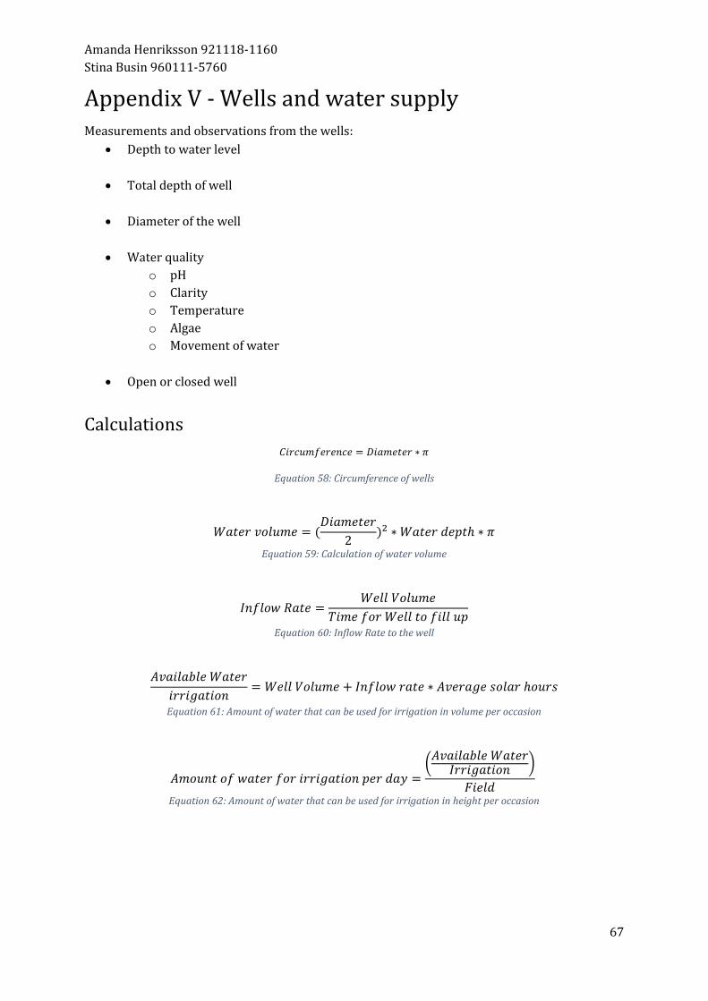
Appendix V - Wells and water supply .................................................................................................... 67 Calculations ............................................................................................................................................................................67


7

List of Charts Chart 1: The harvest year in Machacamarca ....................................................................................................... 18 Chart 2: General and surface inputs for the soil profile of Machacamarca for DSSAT ....................... 29 Chart 3:Layer inputs for the soil profile of Machacamarca for DSSAT ..................................................... 29 Chart 4: Crop management inputs for Experiment file in DSSAT ............................................................... 30 Chart 5: Assumed numbers and prices for the diary ........................................................................................ 31 Chart 6: Standardized well and field ....................................................................................................................... 31 Chart 7: The available amount of water for irrigation ..................................................................................... 32 Chart 8: Harvest yield of barley and alfalfa from simulation of the BAU-scenario .............................. 32 Chart 9: Simulated harvest yield of barley and alfalfa for scenario two .................................................. 33 Chart 10: The amount of times, the average amount and maximum amount of water the crops

need to be irrigated per the simulation ....................................................................................................... 33 Chart 11: Simulated harvest yield of barley and alfalfa for scenario three............................................. 34 Chart 12: The amount of times and total water use per the simulation when the irrigation

amount is limited to 1.33 mm ......................................................................................................................... 34 Chart 13: The amount of harvest left after feeding the cows [kg/ha], calculation method one ..... 37 Chart 14: Number of extra cows it would be possible to feed with irrigation, calculation method

one .............................................................................................................................................................................. 37 Chart 15: Total amount of milk produced per year and hectare [L], calculation method one ........ 38 Chart 16: Total amount of income per year and hectare [BOB], calculation method one ................ 38 Chart 17: Total production of milk, cheese and yoghurt in the dairy per year, calculation method

one .............................................................................................................................................................................. 38 Chart 18: Total income from milk, cheese and yoghurt in the dairy per year [BOB], calculation

method one ............................................................................................................................................................. 39 Chart 19: Final economic income, cost and result for the dairy per year [BOB], calculation

method one ............................................................................................................................................................. 39 Chart 20: Number of cows per hectare, calculation method two ................................................................ 39 Chart 21: Total amount of milk produced per year and hectare [L], calculation method two ....... 40 Chart 22: Total amount of income per year and hectare [BOB], calculation method two ................ 40 Chart 23: Total production of milk, cheese and yoghurt in the dairy per year, calculation method

two .............................................................................................................................................................................. 40 Chart 24: Total income from milk, cheese and yoghurt in the dairy per year [BOB], calculation

method two ............................................................................................................................................................. 40 Chart 25: Final economic income, cost and result for the dairy per year [BOB], calculation

method two ............................................................................................................................................................. 41 Chart 26: Information about the irrigation system........................................................................................... 41 Chart 27: Economic cost of irrigation system ..................................................................................................... 42 Chart 28: Measurements from wells ....................................................................................................................... 68 Chart 29: Further information about the wells .................................................................................................. 68 Chart 30: Standardized field and well .................................................................................................................... 68


8

List of Graphs Graph 1: Seasons in Machacamarca ........................................................................................................................ 19 Graph 2: Average temperature and trend-line for Patacamaya between 1986-2014 ........................ 19 Graph 3: Amount of frost days per month and year between 1986-2014 .............................................. 20 Graph 4: Total precipitation per month and year in mm between 1986-2014 .................................... 20 Graph 5: Minimum temperature and trend line between 1986-2014 ...................................................... 21 Graph 6: Maximum temperature and trend line between 1986-2014 ..................................................... 21 Graph 7: Average radiation per day calculated from the years 2011 – 2014 ....................................... 23 Graph 8: The average harvest yield for barley in kg/ha for the three scenarios for the first period

1986-1988 ............................................................................................................................................................... 35 Graph 9: The average harvest yield for barley in kg/ha for the three scenarios for the second

period 2011-2013 ................................................................................................................................................ 35 Graph 10: The average harvest yield for alfalfa in kg/ha for the three scenarios for the first

period 1986-1988 ................................................................................................................................................ 36 Graph 11: The average harvest yield for alfalfa in kg/ha for the three scenarios for the second

period 2011-2013. ............................................................................................................................................... 36


9

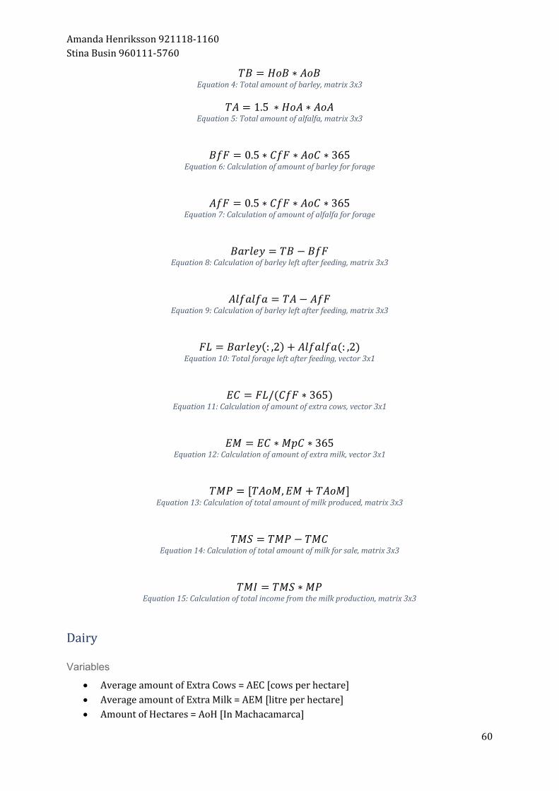
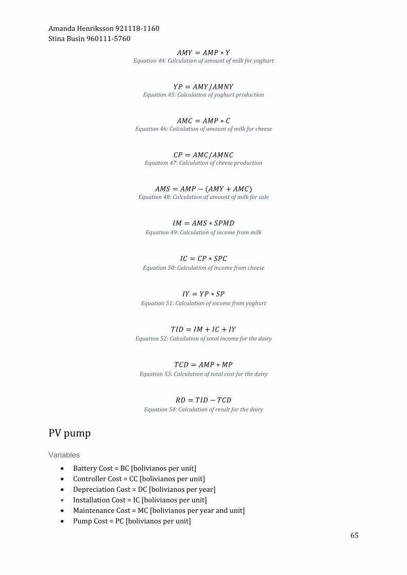
List of Equations Equation 1: Calculation of total amount of milk ................................................................................................. 59 Equation 2: Calculation of consumed milk ........................................................................................................... 59 Equation 3: Calculation of amount of milk for sale ........................................................................................... 59 Equation 4: Total amount of barley, matrix 3x3 ................................................................................................ 60 Equation 5: Total amount of alfalfa, matrix 3x3 ................................................................................................. 60 Equation 6: Calculation of amount of barley for forage .................................................................................. 60 Equation 7: Calculation of amount of alfalfa for forage ................................................................................... 60 Equation 8: Calculation of barley left after feeding, matrix 3x3 .................................................................. 60 Equation 9: Calculation of barley left after feeding, matrix 3x3 .................................................................. 60 Equation 10: Total forage left after feeding, vector 3x1 ................................................................................. 60 Equation 11: Calculation of amount of extra cows, vector 3x1 .................................................................... 60 Equation 12: Calculation of amount of extra milk, vector 3x1 ..................................................................... 60 Equation 13: Calculation of total amount of milk produced, matrix 3x3 ................................................. 60 Equation 14: Calculation of total amount of milk for sale, matrix 3x3 ..................................................... 60 Equation 15: Calculation of total income from the milk production, matrix 3x3 ................................. 60 Equation 16: Calculation of amount of hectares in Machacamarca .......................................................... 61 Equation 17: Calculation of average amount of extra cows .......................................................................... 61 Equation 18: Calculation of average amount of extra milk ............................................................................ 61 Equation 19: Calculation of average amount of milk produced................................................................... 61 Equation 20: Calculation of amount of milk used for yoghurt ..................................................................... 61 Equation 21: Calculation of amount of yoghurt produced ............................................................................. 61 Equation 22: Calculation of amount of milk used for cheese ........................................................................ 62 Equation 23: Calculation of amount of cheese produced ............................................................................... 62 Equation 24: Calculation of amount of milk for sale ........................................................................................ 62 Equation 25: Calculation of income from milk ................................................................................................... 62 Equation 26: Calculation of income from cheese ............................................................................................... 62 Equation 27: Calculation of income from yoghurt ............................................................................................ 62 Equation 28: Calculation of total income for the dairy .................................................................................... 62 Equation 29: Calculation of total cost for the dairy .......................................................................................... 62 Equation 30: Calculation of result for dairy ......................................................................................................... 62 Equation 31: Calculation of total amount of milk consumed ........................................................................ 63 Equation 32: Calculation of total amount of barley, matrix 3x3 .................................................................. 63 Equation 33: Calculation of total amount of alfalfa, matrix 3x3 .................................................................. 63 Equation 34: Calculation of total amount of forage, matrix 3x3 .................................................................. 63 Equation 35: Calculation of amount of forage for one cow per year ......................................................... 63 Equation 36: Calculation of amount of cows that can be fed, matrix 3x3 ................................................ 63 Equation 37: Calculation of amount of milk from exact amount of cows, matrix 3x3........................ 63 Equation 38: Calculation of total amount of milk for sale, matrix 3x3 ..................................................... 63 Equation 39: Calculation of total income from milk, matrix 3x3 ................................................................ 63 Equation 40: Calculation of amount of hectares in Machacamarca ........................................................... 64 Equation 41: Calculation of average amount of milk from rainfed scenario .......................................... 64 Equation 42: Calculation of average amount of milk from irrigated scenario....................................... 64 Equation 43: Calculation of total milk production, vector 2x1 .................................................................... 64 Equation 44: Calculation of amount of milk for yoghurt ................................................................................ 65 Equation 45: Calculation of yoghurt production................................................................................................ 65


10

Equation 46: Calculation of amount of milk for cheese................................................................................... 65 Equation 47: Calculation of cheese production .................................................................................................. 65 Equation 48: Calculation of amount of milk for sale ........................................................................................ 65 Equation 49: Calculation of income from milk ................................................................................................... 65 Equation 50: Calculation of income from cheese ............................................................................................... 65 Equation 51: Calculation of income from yoghurt ............................................................................................ 65 Equation 52: Calculation of total income for the dairy .................................................................................... 65 Equation 53: Calculation of total cost for the dairy .......................................................................................... 65 Equation 54: Calculation of result for the dairy ................................................................................................. 65 Equation 55: Calculation of initial cost for one irrigation system .............................................................. 66 Equation 56: Calculation of depreciation cost for the irrigation system ................................................. 66 Equation 57: Calculation of tube cost ..................................................................................................................... 66 Equation 58: Circumference of wells ...................................................................................................................... 67 Equation 59: Calculation of water volume ........................................................................................................... 67 Equation 60: Inflow Rate to the well ....................................................................................................................... 67 Equation 61: Amount of water that can be used for irrigation in volume per occasion.................... 67 Equation 62: Amount of water that can be used for irrigation in height per occasion ...................... 67


11

Abbreviations BOB - Boliviano (The Bolivian currency1) BAU - Business as usual DSSAT - Decision Support System for Agrotechnology Transfer GDP - Gross Domestic Product INDC - Intended Nationally Determined Contribution IPCC - Intergovernmental Panel of Climate Change SDG - Sustainable development goal UN - United Nations UMSA - Universidad Mayor de San Andrés

1 1 USD = 6,93 BOB (XE, 2018)


12

1 Introduction

1.1 Background The Climate change 2014: Synthesis report, compiled by the Intergovernmental panel of climate change, IPCC, says that “Human influence on the climate system is clear, and recent anthropogenic emissions of greenhouse gases are the highest in history. Recent climate changes have had widespread impacts on human and natural systems.” Both the average global annual land and ocean temperature has increased and the last three decades are most likely the warmest period in the last 1400 years. This has led to a reduced amount of snow and ice on the poles and glaciers worldwide which causes rising sea levels. This have had impact on both natural and human systems globally and has shown how sensitive our systems are to climate change. The new conditions also cause more and stronger extreme weather events like droughts, floods and cyclones which are causing additional stress on the natural and human systems. The threat from climate change is unevenly spread with a greater risk on developing areas and disadvantaged populations. (IPCC, 2014) In 2015, the “2030 agenda for sustainable development” was adopted by the United Nations, UN. The agenda contains 17 sustainable development goals, SDGs, including 169 targets distributed among the different goals on how to achieve a sustainable development. According to the agenda, eradicating poverty is an indispensable requirement and the greatest challenge in the work to achieve a global sustainable development. Shortly after the adoption of the 2030 agenda, the partners of the Climate Convention (UNFCCC) agreed on limiting the global temperature increase to under 2 degrees. To reach the goals of the agenda, governments, companies and the whole of society need to cooperate and act. (United Nations, n.d.) The deployment and use of energy contributes to most greenhouse gas emissions in the world. This makes it an important area to target in the work to limit the global temperature rise and mitigate climate change. 20% of the world’s population lacks access to modern electricity and around 40% still rely on wood, coal and manure for heating and cooking. The lack of access to electricity prevents an economic development as well as exclude part of the world's population. Electricity is a requirement to be able to take part of global health innovations and the lack thereof complicates the work towards a more equal society. It is common in rural areas that women are the ones collecting fuel for the household and this limits their time they can work. It also shortens the time schoolchildren can study to daytime and businesses in the area have a hard time being competitive. Moreover, health clinics cannot provide basic care and vaccination since it in many cases requires cooled storage. (United Nations, n.d.) To decrease the impact of energy and electricity consumption on the greenhouse effect and to secure access to modern energy globally, the share of renewable energy needs to increase in the global energy mix. Infrastructure and technology needs to be expanded and upgraded through international cooperation. (United Nations, n.d) As seen in SDG “Zero Hunger”, small scale farming provides most of the food supply in the developing world. The development of those farms is therefore an important part in the work to eradicate hunger. To be able to supply food for an increasing population simultaneously with a


13

changing climate it requires more resources and modern technology. This will increase the demand of electricity in the developing world, especially in rural areas where many of the agricultural areas are located. To avoid conflicts of interest among the SDGs, it is important to include other relevant goals in the work. Since the electricity demand will increase the targets in SDG “Affordable and clean energy” will be relevant to include, to secure that clean energy is used. These two goals can be achieved with the help of knowledge, financial service and investments in rural infrastructure along with other actions. The agriculture also need a resilience against climate change and the extreme weather conditions this may cause. (United Nations, n.d.) The Andeans in South America are particularly affected by climate change and global warming (Escurra, J.J. et. al. 2014) and is therefore an important region to investigate. This to see how climate change affects local activities and if modern technologies can be used to improve or mitigate the changes. Bolivia is located in the middle west of South America and bordering to Chile, Argentina, Paraguay, Peru and Brazil. The country is characterized by great altitude differences and three different geographical zones. The zones make out of the high Andean region and the Sub-Andean region in the west which constitutes around half of the country and the remaining, in the north and east, is lowland with mainly rainforest. (Central Intelligence Agency, 2018) Bolivia is the poorest country in South America and according to The World Bank, 38.6% of the households lived in poverty the year 2015. The problem is especially big in the Andean region and the rural areas of the country. (The World Bank, 2015) The Bolivian altiplano is mainly occupied by farmers (Yatiña consultora multidisciplinaria S.R.L. 2010) and it is therefore important to investigate the possibilities to improve agricultural conditions so that the communities in these areas does not die out. Agriculture is also an important part of the Bolivian economy and the country export quinoa, soybeans and soy products. (Central Intelligence Agency, 2018) In 2007 agriculture accounted for 13% of the country's total gross domestic product, GDP, which is high if compared to other countries in South America. For example, Peru’s agriculture account for approximately 7.59% and in Brazil it is as low as 5.45%. The agriculture is especially important in rural areas where the economy in some cases depend solely on this. It is also one of the government's focus areas to defeat the widespread poverty in the country (World Bank, 2011) The temperature increase in the Andeans is 0.05 degrees Celsius higher than the global increase which has a negative impact on the mountain range glaciers. Since the glaciers are a main supplier of fresh water to the country there is a risk that the country will suffer from water scarcity as a result of climate change. This will have an impact on the agriculture, mining and other national industries which can cause conflicts over the water reserves among different stakeholders. (Escurra, J.J. et. al. 2014) As part of the process that led to the Paris agreement, Bolivia has developed an Intended Nationally Determined Contribution, INDC, a national document containing actions the country will take toward climate change mitigation and adaptation (World resource institute, n.d). One of the targets in Bolivia’s INDC is to keep the global heating under 1.5 degrees until 2050 (Bolivia, 2015) which is 0.5 degrees lower than the Climate Convention agreed upon. This means that more work needs to be done towards sustainability in all fields.


14

Bolivia has, according to statistics, a fairly low electrification rate compared to other Latin American countries. The total electricity rate in 2017 was around 87%, while urban areas had a rate of 97% and rural areas a rate of 67%. For example, Peru had an electrification rate of 95.1% and Brazil 99.65% (Climate Scope, 2017. (a, b, c) There are two main reasons for this low electrification rate in rural areas; geographic location and poverty rates. Generally, most of the inhabited rural areas have a high poverty rate as well as a geographical location in the Andean region. The Andean region is defined by high altitude and barren landscape, which makes the development of the national grid difficult and costly. (Franziska Buch L. and Leal Filho W., 2012)

1.2 Field study area - Machacamarca, Bolivia Machacamarca is a canton located in the municipality of Colquencha, in the province Aroma which is a part of the department of La Paz. Machacamarca is divided in communities named Machacamarca, Chullumpiri, Collmini, Escohoco, Kamani and Posokani. The canton is in the altiplano area 54 km south of La Paz. The terrain of the canton is only plains with an altitude of approximately 3900 meter above sea level. There is a permanent river that flows through all the six communities called Jacha Jawira, in each of the communities there are temporary rivers that exist during rainy season only. In the community of Kamani there is also a small lake. The rivers and the lake supplies cattle with water and in some cases, they are also used for irrigation. All the communities except Kamani has permanent water supply from wells that are used for human consumption. The wells in Kamani is usually dry from November to January. (Yatiña consultora multidisciplinaria S.R.L. 2010) The main occupation in the canton is cultivation of crops, like barley, alfalfa and oats, cattle raising as well as the production and processing of milk. The milk production is highly dependent on the production of barley and alfalfa because these are the main food source for the milk cows. The population of the canton is approximately 1800 people, evenly distributed between men and women with most the population between the ages of 20 to 59. (Yatiña consultora multidisciplinaria S.R.L. 2010) The electrification rate in Machacamarca is approximately 42.5%, which is an average between the six communities (Yatiña consultora multidisciplinaria S.R.L. 2010). The main energy consuming activities in Machacamarca is cooking and milk processing, which are two activities that are easy to do without electricity. The canton has connection to the national electricity grid but not all the houses are connected because it entails a high cost. The families that do not have access to the electricity grid uses manure, liquid gas and firewood for cooking. The use of liquid gas is limited to the rain periods when the ordinary fuelwood is too humid. Liquid gas is otherwise considered too expensive to be used all year around. (Huallapara Lliully, A. T., 2015)

1.1.3 Smart Ayllu This thesis is a part of a bigger project led by Universidad Mayor de San Andrés, UMSA, in La Paz, Bolivia. The project is called Smart Ayllu, which means smart community in aymara, an indigenous language spoken in the area. The projects overall purpose is to “Maximize the impact of efficient use of the energy for social- and development-benefits”. It consists of a range of interdisciplinary projects that focuses on energy, education, health, secure food, water and environment within the production areas mining, agriculture, cattle and crafts in the


15

municipality of Colquencha. In the center of the project, there is a constant dialogue with the community to make sure their needs and cultural heritage is meet. (UMSA, 2017)


16

2 Research scope

2.1 Purpose The main purpose of this study is “to evaluate the impact of implementing photovoltaic water pumps on production and economic development in the canton of Machacamarca in Bolivia. The canton is dependent on agriculture, and harvest yields have become more irregular due to climate change and resulting weather conditions.

2.2 Objectives x Evaluate the costs of implementing photovoltaic water pumps for irrigation x Evaluate the difference in crop yield and the economic effect of this x Assess if the dairy would be affected by an implementation of irrigation x Evaluate the economic feasibility to implement photovoltaic water pumps for irrigation

2.3 Research question How much can the agricultural production in Machacamarca increase and be stabilized through the use of photovoltaic water pumps. What economic improvement and social impacts could this have in the canton?

2.4 Relevance Bolivia‘s INDC gives the country a range of targets to work towards. They want to eradicate extreme poverty which forces them to develop the national economy at the same time as they work against further impact on the climate. The country will have a full electricity cover to 2025 with an increased share of renewable. The forestry and agriculture will be increased and strengthen through adaption to the changing climate and the use of technologies (Bolivia, 2015). This project focuses mostly on the agricultural sustainability since this is the main income in Machacamarca. In this case irrigation driven by photovoltaic energy, will be evaluate as a technology to adapt the agriculture to climate changes, as well as assess how this could contribute to the SDGs. A sustainable agriculture and an opportunity to clean energy does not only give environmental advantage but also economic and social stability, especially in the canton of Machacamarca.

2.5 Delimitation This thesis is limited to evaluating one canton in the municipality of Colquencha, named Machacamarca. Within this canton the thesis will only focus on the production of crops; alfalfa and barley which are the main forage sources for the milk cows in the canton and available crops in the simulation program “Decision support system for agrotechnology transfer”, DSSAT. Furthermore, the thesis will evaluate the relationship between cereal production and milk production. The income calculated for the farmers is limited to the milk their cows produce and for the dairy it is limited to their three products; processed milk, yoghurt and cheese.


17

3 Facts

3.1 Bolivia and Machacamarca Bolivia is an old Spanish colonial and gained independence in 1825. The country has not had an easy development since and its history is filled with conflicts both within the country and with its neighbors. (Central Intelligence Agency, 2018) Many of the conflicts in the country derives from the big interest of natural resources that is found in plenty here. One of these conflicts, in 1879-1884, resulted in Bolivia losing its only connection to the ocean when Chile took control over an area with large copper deposits. The fact that Bolivia is a landlocked country makes export and import trade very difficult when it comes to the resources the country still control. One example of this is when Bolivia started an export trade of natural gas to the United States and Chile ended up making more money from this. The reason for this was that they had to use Chiles port for the export, a piece of land that used to belong to Bolivia. (Arnson, Fuentes and Aravena, 2008) The political situation has over the years been very unstable and Bolivia has had times of dictatorship. This has increased the economic difficulties the country has suffered and it has suppressed the development of the poor and rural areas. The political difficulties remain today and there are claims of corruption and discrimination of the indigenous populations. (Central Intelligence Agency, 2018)

3.1.1 Energy Situation Bolivia's current energy mix consists of 77% fossil fuels, with an installed capacity of approximately 1.9 GW. The country is 100% self-sufficient in energy distribution and export some of its energy resources. Most of the fossil fuels comes from natural gas which the country has great access to. (Climate Scope, 2017) Despite the issues connected with electrifying Bolivia, the government has set a goal that by 2030 the whole population should be electrified (United Nations (a), n.d). But so far they have not set up any plans or policies of how this should be done. According to the simulation tool, ”Universal Access to Electricity”, a tool developed by the UN to find the best electrification option to the lowest cost, the cheapest way to electrify the rest of Bolivia would be through standalone photovoltaic technology (United Nations (b), n.d). To electrify Bolivia through the use of the national grid will be technically difficult and expensive considering how the country looks geographically. Therefore, it is important to find financially sustainable technologies to replace the national grid in the most inaccessible regions. (Franziska Buch L. and Leal Filho W., 2012)

3.1.2 Agriculture The existing agriculture is in many ways outdated and based on traditions handed down through generations and therefore often lack efficiency measures. This shows clearly in the productivity. Bolivia has one of the lowest productivity rates in Latin America. In many cases the irrigation is solely dependent on rainfall and lack supporting technologies. (World Bank, 2011)


18

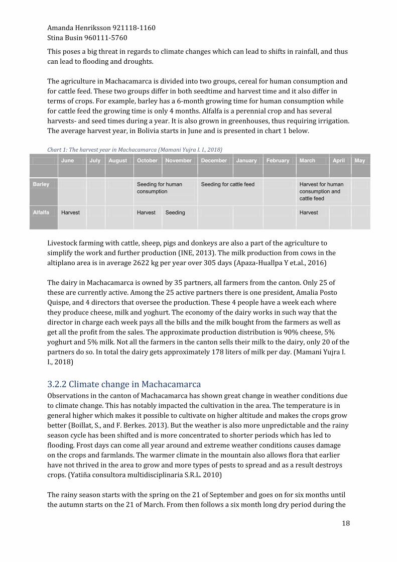
This poses a big threat in regards to climate changes which can lead to shifts in rainfall, and thus can lead to flooding and droughts. The agriculture in Machacamarca is divided into two groups, cereal for human consumption and for cattle feed. These two groups differ in both seedtime and harvest time and it also differ in terms of crops. For example, barley has a 6-month growing time for human consumption while for cattle feed the growing time is only 4 months. Alfalfa is a perennial crop and has several harvests- and seed times during a year. It is also grown in greenhouses, thus requiring irrigation. The average harvest year, in Bolivia starts in June and is presented in chart 1 below. Chart 1: The harvest year in Machacamarca (Mamani Yujra I. I., 2018)

June July August October November December January February March April May

Barley Seeding for human consumption

Seeding for cattle feed Harvest for human consumption and cattle feed

Alfalfa Harvest Harvest Seeding Harvest

Livestock farming with cattle, sheep, pigs and donkeys are also a part of the agriculture to simplify the work and further production (INE, 2013). The milk production from cows in the altiplano area is in average 2622 kg per year over 305 days (Apaza-Huallpa Y et.al., 2016) The dairy in Machacamarca is owned by 35 partners, all farmers from the canton. Only 25 of these are currently active. Among the 25 active partners there is one president, Amalia Posto Quispe, and 4 directors that oversee the production. These 4 people have a week each where they produce cheese, milk and yoghurt. The economy of the dairy works in such way that the director in charge each week pays all the bills and the milk bought from the farmers as well as get all the profit from the sales. The approximate production distribution is 90% cheese, 5% yoghurt and 5% milk. Not all the farmers in the canton sells their milk to the dairy, only 20 of the partners do so. In total the dairy gets approximately 178 liters of milk per day. (Mamani Yujra I. I., 2018)

3.2.2 Climate change in Machacamarca Observations in the canton of Machacamarca has shown great change in weather conditions due to climate change. This has notably impacted the cultivation in the area. The temperature is in general higher which makes it possible to cultivate on higher altitude and makes the crops grow better (Boillat, S., and F. Berkes. 2013). But the weather is also more unpredictable and the rainy season cycle has been shifted and is more concentrated to shorter periods which has led to flooding. Frost days can come all year around and extreme weather conditions causes damage on the crops and farmlands. The warmer climate in the mountain also allows flora that earlier have not thrived in the area to grow and more types of pests to spread and as a result destroys crops. (Yatiña consultora multidisciplinaria S.R.L. 2010) The rainy season starts with the spring on the 21 of September and goes on for six months until the autumn starts on the 21 of March. From then follows a six month long dry period during the


19

autumn and winter until the 21 of September with the driest period in the end of the winter. The seasons are displayed in graph 1 below.

Graph 1: Seasons in Machacamarca (Mamani Yujra, I I. 2018)

An analysis from the weather station called Patacamaya, located in the same region as the canton of Machacamarca, shows that the weather has changed since 1986. An analysis of total precipitation per month, average temperature per year and amount of frost days per month has been made. The average temperature increase between the years 1986 and 2014 is as much as 2.1 degrees Celsius. Compared to the average temperature increase of the whole earth in the same time-period it is an extreme increase. According to observations from NASA the average increase in temperature during this time period is only 0.55 degrees Celsius (NASA, 2018). The average temperatures per year is shown in graph 2 below including a trend-line of how the average temperature has changed over the years.

Graph 2: Average temperature and trend-line for Patacamaya between 1986-2014 (Patacamaya, 2016)

0.0 2.0 4.0 6.0 8.0

10.0 12.0

DEGR

EES C

ELSI

US

YEAR

AVERAGE TEMPERATURE - PATACAMAYA

AVERAGE TEMPERATURE

TRENDLINE


20

Amount of frost days per month has decreased as a result of increased temperatures. This affects the production of Chuños, which is an ancient technique of making a toxic type of potato edible, which needs to be left out during a certain amount of days with frost (The Smithsonian, 2011). The average decrease in frost days per month during the time-period 1986 to 2014 is 6.7 days with the highest being in October with a decrease of 18 days and the lowest in December with a decrease of 1 days. The amount of frost days per month is shown in graph 3 below.

Graph 3: Amount of frost days per month and year between 1986-2014 (Patacamaya, 2016)

The precipitation per month does not, as clearly as frost days and temperature, show evidence of climate change. But nevertheless, it shows an irregularity in rain which means that the planning of agriculture is made difficult. The average decrease of precipitation per month is 12.7 mm with the highest decrease in December with a decrease of 130.2 mm and highest increase in September with 48.2 mm. The amount of precipitation per month is shown in graph 4 below.

Graph 4: Total precipitation per month and year in mm between 1986-2014 (Patacamaya, 2016)


21

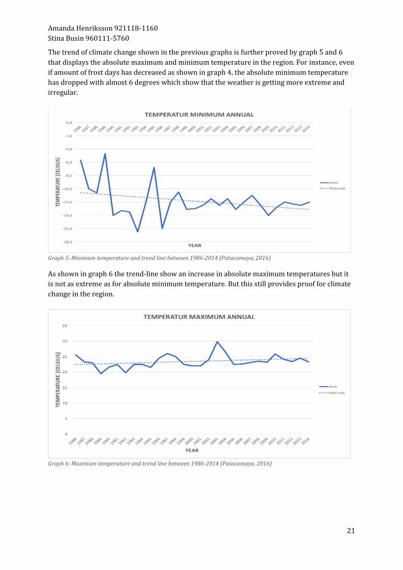
The trend of climate change shown in the previous graphs is further proved by graph 5 and 6 that displays the absolute maximum and minimum temperature in the region. For instance, even if amount of frost days has decreased as shown in graph 4, the absolute minimum temperature has dropped with almost 6 degrees which show that the weather is getting more extreme and irregular.

Graph 5: Minimum temperature and trend line between 1986-2014 (Patacamaya, 2016)

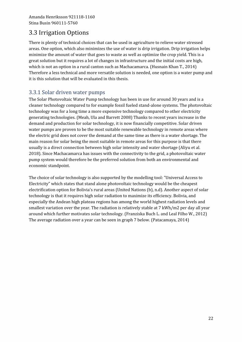
As shown in graph 6 the trend-line show an increase in absolute maximum temperatures but it is not as extreme as for absolute minimum temperature. But this still provides proof for climate change in the region.

Graph 6: Maximum temperature and trend line between 1986-2014 (Patacamaya, 2016)


22

3.3 Irrigation Options There is plenty of technical choices that can be used in agriculture to relieve water stressed areas. One option, which also minimizes the use of water is drip irrigation. Drip irrigation helps minimize the amount of water that goes to waste as well as optimize the crop yield. This is a great solution but it requires a lot of changes in infrastructure and the initial costs are high, which is not an option in a rural canton such as Machacamarca. (Husnain Khan T., 2014) Therefore a less technical and more versatile solution is needed, one option is a water pump and it is this solution that will be evaluated in this thesis.

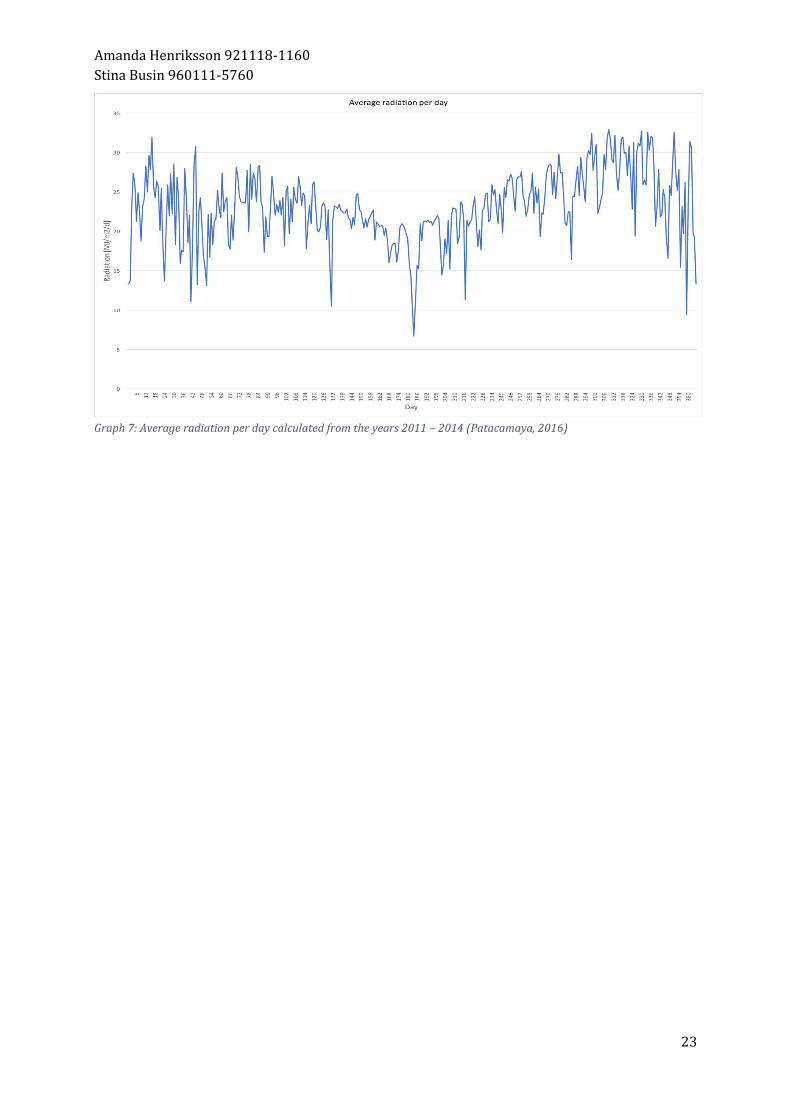
3.3.1 Solar driven water pumps The Solar Photovoltaic Water Pump technology has been in use for around 30 years and is a cleaner technology compared to for example fossil fueled stand-alone systems. The photovoltaic technology was for a long time a more expensive technology compared to other electricity generating technologies. (Meah, Ula and Barrett 2008) Thanks to recent years increase in the demand and production for solar technology, it is now financially competitive. Solar driven water pumps are proven to be the most suitable renewable technology in remote areas where the electric grid does not cover the demand at the same time as there is a water shortage. The main reason for solar being the most suitable in remote areas for this purpose is that there usually is a direct connection between high solar intensity and water shortage (Aliyu et al. 2018). Since Machacamarca has issues with the connectivity to the grid, a photovoltaic water pump system would therefore be the preferred solution from both an environmental and economic standpoint. The choice of solar technology is also supported by the modelling tool: ”Universal Access to Electricity” which states that stand alone photovoltaic technology would be the cheapest electrification option for Bolivia's rural areas (United Nations (b), n.d). Another aspect of solar technology is that it requires high solar radiation to maximize its efficiency. Bolivia, and especially the Andean high plateau regions has among the world highest radiation levels and smallest variation over the year. The radiation is relatively stable at 7 kWh/m2 per day all year around which further motivates solar technology. (Franziska Buch L. and Leal Filho W., 2012) The average radiation over a year can be seen in graph 7 below. (Patacamaya, 2014)


23

Graph 7: Average radiation per day calculated from the years 2011 – 2014 (Patacamaya, 2016)


24

4 Methodology

4.1 Interviews To find local knowledge, interests and to receive support for the necessary assumptions interviews will be held with local interest groups and people with expertise in the different areas. A semi-structured interview form will be used which includes some predefined questions but has an open ending to be able to gain further information about the subject (Wilson C., 2014). Different questions are prepared to the different interviews but depending on the answers and the person that is interviewed will the following question vary. This also makes it easier to adapt the interview in situations where the person may not want or cannot answer every question. The interview questions will be revised by the professors at UMSA to avoid inappropriate questions and the interviewed farmers will be anonymous. They will be anonymous to be able to protect their integrity. The interviews are going to be used to complement the literature study that has been made. The facts expected from the interviews with the farmers in Machacamarca are firstly the farmers own experience of climate change and how that has affected their cultivation. In addition to this the farmer’s own knowledge about the cultivation in the area, the size of their agriculture, amount of milk cows and the relationship between consumed forage and produced milk. In the interviews with the expert’s specific numbers, costs and facts within their expert field are expected to be found. These are for example cost and sales prices for the dairy, cultivation management parametric and pump details. More specifically, the photovoltaic water pump, will be studied to find what type and size that would be suited for the local conditions found from observations. Internal and maintenance costs for the chosen pump will be determined to use in later economical simulations. The result will be used in the report and the asked questions and important parts of the interviews will be presented in appendix I and II.

4.1.1 Experts This thesis has been made possible by the help of three experts from different fields. These experts have continuously provided information during the field study to be able to make necessary decisions. Below is a presentation of these people to get a better understanding why they are important to this thesis. Isaac Ivan Mamani Yujra, Agricultural engineer at UMSA in La Paz, Bolivia. Isaac is currently writing a thesis about the cultivation of potatoes, barley, quinoa and cañahua in the municipality of Colquencha to evaluate if it is profitable for the economy of the cantons. The study includes territorial-, soil and management aspects. (Mamani Yujra, I. I. 2018) Reinhard Mayer Falk is a physics professor who now is the technical manager of the company EcoEnergía FALK located in La Paz, a solar panel company that works a lot with rural areas. (EcoEnergía FALK, 2018)


25

Amalia Posto Quispe is the president of the local dairy of Machacamarca. She oversees the dairy and makes sure everything runs smoothly. She has the greatest knowledge of the dairy in Machacamarca. (Posto Quispe A., 2018)

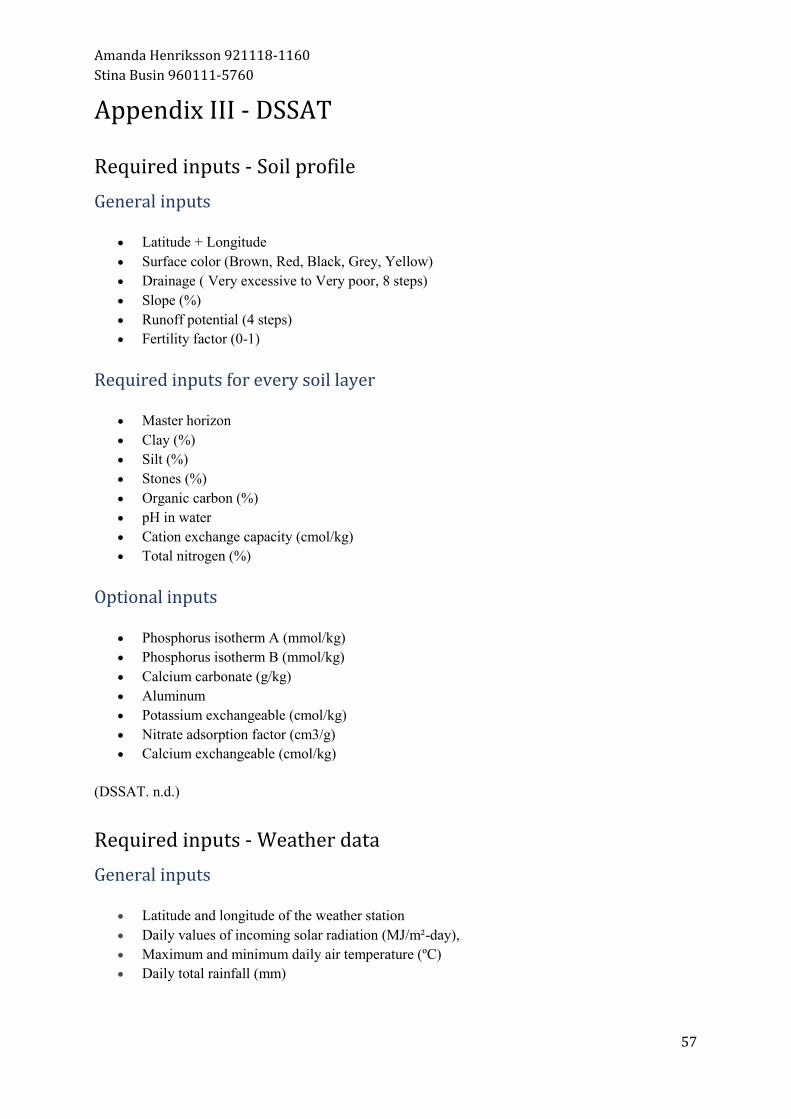
4.2 Simulation programs The following information is regards to the simulation programs used in the thesis, DSSAT 4.7 and Matlab version R205b. The input and output data required will be presented in appendixes.

4.2.1 Decision support system for agrotechnology transfer DSSAT, developed by International Benchmark Sites Network for Agrotechnology Transfer (Jones, J.W. et.al. 2003) is a software program that simulate crop grow, development and yield as a function from the required inputs. The newest version, 4.7, includes data for 42 different crops and in addition to this the program needs site specific daily weather data, soil profile and crop management data. The program then combines the inputs and it is possible to adjust and create “What if” simulations. The necessary parameters can be found in appendix III. (DSSAT. n.d.) This simulation program will be used to simulate three different agricultural scenarios for two time periods for each of the two crops; barley and alfalfa. The first scenario will be a “business as usual”- scenario, BAU, where the cultivation only is rainfed. In the second scenario, an irrigation system will be introduced that will irrigate an ideal amount of water when required. This to be able to see how much water is needed and the maximum possible harvest yield, which is useful for occasions when the water level is higher than usual. In the third scenario, an irrigation system will also be implemented and irrigate automatically when required but this time with a limited amount of water based on the local conditions. To enable this standardized fields, wells and water supply will be created based on the completed observations and interviews. The four first and the four last years of the available weather data, 1986-1989 and 2011-2014 will be used in the simulations. The outcome from the two time-periods will then be compiled to find an average increase in crop yield the irrigation will lead to. The two time-periods will later be compared to see how the change in weather has affected the agriculture and if an implementation of an irrigation system has greater impact in any of the time periods.

4.2.2 Matlab The Matlab code is written for this thesis and is used to be able to calculate the economic impact of implementing water pumps. The input data used in the calculations is retrieved from interviews and observations during the field study as well as from literature studies. The output from the simulation program is used as part of the input data in this code. The output from the code will be plotted and analyzed. The economic variables that will be taken into consideration is cost for the water pumps, milk cost and sales cost for the products in the dairy. More specifically for the water pumps this includes installation cost, cost for unit, maintenance cost and system cost. There are other economic variables to consider when cultivating, for example cost for transport, fertilizer, pesticide, crops and so on. But in Machacamarca the farmer's does not use fertilizers, pesticides or transportation and the value for crop cost was not possible to determine. Therefore, it is not


26

considered in this thesis and gives an error in the calculations. A complete list of inputs, outputs and calculations can be found in appendix IV. In the Matlab-simulation, the crop production will be set in a relation with the amount of produced milk to see how a changed forage production could impact on the milk production. This will be transferred into an economical simulation to evaluate the impact on the income for the cantons farmers and the local dairy. When the economic aspects are assessed a final analysis will be done to evaluate if it is economically sustainable to implement a photovoltaic irrigation system in the agriculture in the canton of Machacamarca. In the Matlab simulation there is two different calculation methods, one and two. Calculation method one is mainly based on input-data retrieved from interviews and method two is mainly based on input data from the DSSAT-simulations

4.3 Assumptions There has been made a few assumptions in this thesis to be able to make calculations and to come to a conclusion. The assumed numbers and facts are based on interviews, previous research and observations from the field study. An average field, dairy producing livestock number and daily milk production will be created from observations and interviews to use in the simulation programs. It is also assumed that all the cultivated areas are used to grow alfalfa and barley for forage. This to receive a clearer result that is easier to compare. The required inputs to the simulation program DSSAT and the economic simulation will be determined based on results from the field study and assumed to apply throughout the whole canton. The assumed inputs and values can be found in the result section. The BAU-scenario will have a fixed amount of milk cows, in calculation method one, determined from the field observations. This will give a constant milk production and forage demand which some years may mean that it requires purchase of forage when the simulated harvest yield is not sufficient. Those costs will not be considered in the economical simulation. In Matlab, when calculating over a year, leap years has not been taken into consideration. This, to simplify the calculations.


27

5 Results

5.1 Interviews Farmers and people living in Machacamarca who were willing to answer some questions got interviewed during the field study. Questions about cultivation, cattle, milk production and the dairy were asked. The perception of climate change and the possible impact that has had on the agriculture was also inquired during the interviews. The answers from the different framers were compared and some averages values were created to be able to use as input data in the simulations. The generated values correctness is later compared and discussed to found data in earlier studies. The interviewed farmers were also asked if they had wells on their properties and if they did, measurements were taken on these. The questions and references for this section is presented in appendix I and II respectively.

5.1.1 Interviews with farmers and measurements The results from the interviews show that the consensus towards climate change is that it is affecting the crop yield, especially with an interference in the rain. This has affected the crop yield, and one farmer testified to one of his buildings being destroyed from the rains. The consensus is also that an irrigation system would improve the agriculture in the canton and ultimately improve the milk production or the income from selling the leftover crop yield. (Annon, (1-5), 2018) The type of crops cultivated in the canton varies a little between the families and is mostly dependent on the size of their land. But the most commonly cultivated crops are oats, alfalfa and barley. These crops are mainly used to feed the milk cows, but in some cases the harvest is also used for self-consumption or as an extra income by selling it at the nearby market. It is mainly families with large land and a high production yield that has the possibility to use it for food or sell it. (Annon, (1-5), 2018) The farmers in Machacamarca has a cultivation area of a ⅕ to 5 hectares and between 2 and 20 milk cows. These big differences are due to big differences in income between the different families. The cows are feed approximately two armfuls of forage per day. The cows produce approximately 7 liters of milk per day but this varies depending on how much forage the cow is feed, which in turn is dependent on the crop yield. (Annon, (1-5), 2018) From these interviews, input values have been created for the simulations. All the farmers that were interviewed had at least one well and these were measured according to the data required to be able to choose a suitable water pump and irrigation system. The measurements made on each well is presented in appendix V.

5.1.2 Interview with the president of the dairy Only 20 of the families that have milk cows sells the milk from their cows each day at the local cooperative dairy factory for 3 bolivianos per liter. The dairy factory gets approximately 170 liters of milk each day from the farmer. The factory processes the milk and produce 3 different types of cheese, yoghurt and milk. Approximately 40% of the unprocessed milk goes to milk,


28

30% to yoghurt and 30% to the 3 different types of cheese. These products are sold at the local market and some of the products gets sold back to the farmers. The price for the milk is 4 bolivianos per liter, for yoghurt it is 8 bolivianos per liter and for the cheese the price is approximately 24 bolivianos per kilogram. 5.1.3 Interview with owner of EcoEnergía FALK The chosen pump for the water requirement and well dimensions is the Shuflu 8000 together with a 130 W solar panel and a 12 V battery to improve the usage time from five to seven hours and to stabilize the pump. The pump will be able to maintain a water flow of 348 liters per hours which makes a total of 2436 liters per day. This is a bit lower than the required but the next pump size has a too big water flow and has a higher cost. To make the system work properly the parts are installed to a control board with an electric regulator, a mast for the solar panel and a table for the battery and pump. The pump is 21 cm long, 8 cm wide and weights 1.9 kg. It has a two year guaranty and has a regular maintenance need every second year when a membrane needs to be changed. It is an easy task and can be completed by the owner without further expertise. The costs and technical life span for the different system parts are presented in chart 26.


29

5.2 Input data 5.2.1 Soil profile The general and surface inputs of the soil profile from Machacamarca is presented in chart 2. The soil profile for the simulation consists of two layers with a thickness of 33 cm and 124 cm to a total depth of 157 cm. The inputs for the two layers are presented in chart 3. Chart 2: General and surface inputs for the soil profile of Machacamarca for DSSAT. (Chambi Tapia, M I. 2017)

General and surface inputs

Longitude and Latitude 16°52'37.92" S, 68°12'20.16" W

Surface color Brown

Drainage Moderately well

Slope 1%

Runoff potential Moderately low

Fertility factor 0,2

Chart 3:Layer inputs for the soil profile of Machacamarca for DSSAT. (Chapman S. 2012) (Chambi Tapia, M I. 2017) (Enríquez, S. et. al. 2016)

Layer 0-33 cm 33-157 cm

Master horizon A B

Clay (%) 14 26

Silt (%) 82 65

Organic carbon (%) 4 9

pH in water 1.13 0.039

Cation exchange capacity (cmol/kg) 3.53 3.53

Total nitrogen (%) 0.095 0.095

Phosphorus isotherm A (ppm) 14.08 7.26

Phosphorus isotherm B (mmol/kg) No data No data

Calcium carbonate (g/kg) 3.53 3.53

Aluminum No data No data

Potassium exchangeable (cmol/kg) No data No data

Nitrate adsorption factor (cm3/g) No data No data

Calcium exchangeable (cmol/kg) No data No data


30

5.2.2 Crop management The crop management inputs for the cultivation of alfalfa and barley are presented in chart 4. Chart 4: Crop management inputs for Experiment file in DSSAT. (Mamani Yujra, I. I. 2018. Rankin M, 2008. Queensland government. 2012)

Inputs Alfalfa Barley

Planting date 15 of November 15 of November

Planting method Dry seeds Dry seeds

Planting distribution Rows Rows

Plant population at seeding

800 plants/m2 100 plants/m2

Row spacing 10 cm 20 cm

Row direction for north 0° 0°

Planting depth 0.5 cm 2 cm

Management depth irrigation

30 cm 30 cm

Harvest date 15 of March and 15 of July* At maturity

*Alfalfa is harvested 3 times a year, the harvest yield will be multiplied by 1.5 in the economical simulation.

5.2.3 Weather data The weather data is received from the weather station in Patacamaya, located 50 km south of Machacamarca at an elevation of 3793 m. The weather data is in monthly averages and since daily data is required in the program, the monthly figures for maximum and minimum temperatures has been used for everyday of that month. The precipitation over a month has been given in average rainfall in mm and amount of days with rain in that month. The average rainfall has been randomly placed over the month according to the amount of rain days. The solar radiation data from the area is a daily average from the years 2011-2014. The solar radiation value for every day has been randomly selected from the average values from the correct month.


31

5.2.4 The dairy production The assumed numbers and prices for the dairy, based on interviews are presented in chart 5. Chart 5: Assumed numbers and prices for the diary (Posto Quipse A., 2018)

Assumptions

Amount of milk cows [pcs/hectare] 2

Amount of milk [L/cow/day] 7

Amount of forage [kg/cow/day] 10

Purchase price for milk for the dairy [BOB/L] 3

Sales price milk [BOB/L] 4

Sales price cheese [BOB/kg] 24

Sales price yoghurt [$/L] 8

Amount of milk for 1 kg cheese [L/kg] 10

Amount of milk for 1 L yoghurt [L/L] 1.5

5.2.5 The standardized wells and fields An average well with a corresponding field has been calculated from measurements on four wells in Machacamarca. The values are presented in chart 6. See measurements and calculations in appendix V. Chart 6: Standardized well and field

Standard well and field

Diameter [m] 1.1

Total depth [m] 3.9

Depth to water [m] 1.8

Water depth [m] 2.1

Inflow [m³/h] 0.17

Volume [m³] 2.0

Field size [ha] 0.25


32

5.2.6 Irrigation possibilities The available amount of water for irrigation for the standardized field from the standardized well is presented in chart 7. Calculations can be found in appendix V. Chart 7: The available amount of water for irrigation

Field [ha]

Volume [m3]

Flow [m3/h]

Average irrigation hours [h]

Total amount of available water per irrigation [m3]

Possible irrigation per day [mm/day]

0.25 1.98 0.17 8 3.34 1.33

5.3 Simulations 5.3.1 Scenario one - Business as usual Chart 8 presents the harvest yield of barley and alfalfa from the BAU-scenario, that only is rainfed. Chart 8: Harvest yield of barley and alfalfa from simulation of the BAU-scenario

Rainfed Barley [kg/ha/year] Alfalfa* [kg/ha/year]

1986 5 465 4 807.5

1987 951 6 063

1988 442 0

Average 2 286 5 435.25

2011 1 730 5 071.5

2012 4 533 5 599.5

2013 4 695 2 827.5

Average 3 652.67 4 499.5 *The simulated value has been multiplied by 1.5 to get the harvest yield for all three harvests over a year. The average production of barley in the canton of Machacamarca on the year of 2013 were per measurements made by Instituto Nacional de Estadística 2680.14 kg per hectare and 3397.48 kg per hectare for alfalfa. (INE, 2013)


33

5.3.2 Scenario two – Ideal irrigation, when required In chart 9 the simulated harvest yield of barley and alfalfa is presented for the second scenario with ideal irrigation. Chart 10 presents the irrigation requirement for the two crops with average required amount of water, amount of irrigation occasions and the maximum water need. Chart 9: Simulated harvest yield of barley and alfalfa for scenario two

Ideal irrigation Barley [kg/ha/year] Alfalfa [kg/ha/year]

1986 5 465 7 380

1987 951 7 682

1988 442 7 509

Average 5 560 7 524

2011 1 730 8 610

2012 4 533 8 288

2013 4 695 8 436

Average 5 650 8 445

Chart 10: The amount of times, the average amount and maximum amount of water the crops need to be irrigated per the simulation

Irrigation Times, Alfalfa Total amount of water, Alfalfa [mm]

Times, Barley

Total amount of water, Barley [mm]

1986 11 355.2 3 116.1

1987 8 257.9 3 106

1988 16 512 7 235.1

Average 11.67 32.18 4.33 35.87

Maximum 16 55.1 55.1

2011 11 353.8 3 218.6

2012 8 245.8 2 156.3

2013 13 407.3 2 153.4

Average 11 31.4 2 75.9

Maximum 13 58.6 88.9


34

5.3.3 Scenario three - Limited automatic irrigation when required In chart 11 the harvest yield for barley and alfalfa is presented from the simulation of the third scenario, when the amount of water per irrigation is limited to 13.4 mm from calculations presented in chart 7. In chart 12 the amount of irrigation occasions is presented as well as total water use over the cultivation period. Chart 11: Simulated harvest yield of barley and alfalfa for scenario three

Limited irrigation Barley [kg/ha/year] Alfalfa [kg/ha/year]

1986 5 919 6 933

1987 4 501 7 590

1988 4 120 4 238

Average 4 847 6 254

2011 5 454 7 008

2012 6 351 7 419

2013 5 190 5 426

Average 5 665 6 618

Chart 12: The amount of times and total water use per the simulation when the irrigation amount is limited to 1.33 mm

Times, Alfalfa

Total amount of water, Alfalfa [mm]

Times, Barley

Total amount of water, Barley [mm]

1986 155 206 155 206

1987 168 223 168 223

1988 244 324 244 325

Average 189 251 189 251

2011 171 227 171 227

2012 159 211 159 211

2013 187 249 187 249

Average 172 229 172 229


35

5.3.4 Average harvest yields The average harvest yield for the three scenarios in the two time-periods for barley and alfalfa are shown in graph 8 to 11. In graph 8, the improvement from the BAU-scenario is 143% for scenario 2 and 112% for scenario 3.

Graph 8: The average harvest yield for barley in kg/ha for the three scenarios for the first period 1986-1988

In graph number 9, the improvement from the BAU-scenario is 55% for both scenario 2 and 3.

Graph 9: The average harvest yield for barley in kg/ha for the three scenarios for the second period 2011-2013

In graph 10, the improvement from the BAU-scenario is 108% to scenario 2 and 73% for scenario 3.


36

Graph 10: The average harvest yield for alfalfa in kg/ha for the three scenarios for the first period 1986-1988

In graph 11, the improvement from the BAU-scenario is 88% for scenario 2 and 47% for scenario 3.

Graph 11: The average harvest yield for alfalfa in kg/ha for the three scenarios for the second period 2011-2013.

5.4 Economic outcome Below the results from the Matlab-simulations will be presented in two different sections. The first section is the economic and milk production outcome per hectare from the simulations in DSSAT for the BAU-scenario and the scenario with restricted irrigation. The second section is the economic outcome for the dairy, and this includes the total arable area in the canton.


37

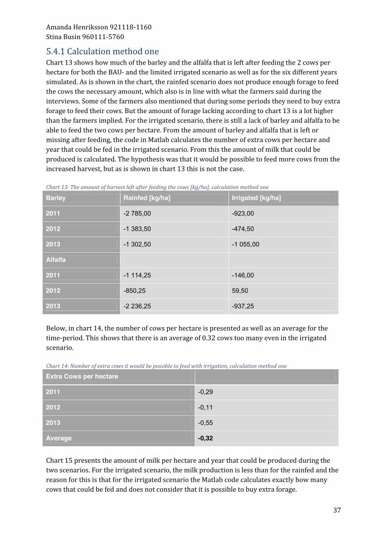
5.4.1 Calculation method one Chart 13 shows how much of the barley and the alfalfa that is left after feeding the 2 cows per hectare for both the BAU- and the limited irrigated scenario as well as for the six different years simulated. As is shown in the chart, the rainfed scenario does not produce enough forage to feed the cows the necessary amount, which also is in line with what the farmers said during the interviews. Some of the farmers also mentioned that during some periods they need to buy extra forage to feed their cows. But the amount of forage lacking according to chart 13 is a lot higher than the farmers implied. For the irrigated scenario, there is still a lack of barley and alfalfa to be able to feed the two cows per hectare. From the amount of barley and alfalfa that is left or missing after feeding, the code in Matlab calculates the number of extra cows per hectare and year that could be fed in the irrigated scenario. From this the amount of milk that could be produced is calculated. The hypothesis was that it would be possible to feed more cows from the increased harvest, but as is shown in chart 13 this is not the case. Chart 13: The amount of harvest left after feeding the cows [kg/ha], calculation method one

Barley Rainfed [kg/ha] Irrigated [kg/ha]

2011 -2 785,00 -923,00

2012 -1 383,50 -474,50

2013 -1 302,50 -1 055,00

Alfalfa

2011 -1 114,25 -146,00

2012 -850,25 59,50

2013 -2 236,25 -937,25

Below, in chart 14, the number of cows per hectare is presented as well as an average for the time-period. This shows that there is an average of 0.32 cows too many even in the irrigated scenario. Chart 14: Number of extra cows it would be possible to feed with irrigation, calculation method one

Extra Cows per hectare

2011 -0,29

2012 -0,11

2013 -0,55

Average -0,32

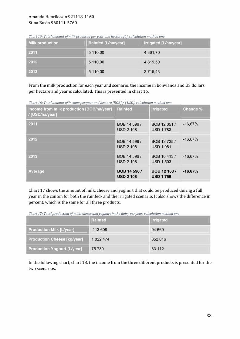
Chart 15 presents the amount of milk per hectare and year that could be produced during the two scenarios. For the irrigated scenario, the milk production is less than for the rainfed and the reason for this is that for the irrigated scenario the Matlab code calculates exactly how many cows that could be fed and does not consider that it is possible to buy extra forage.


38

Chart 15: Total amount of milk produced per year and hectare [L], calculation method one

Milk production Rainfed [L/ha/year] Irrigated [L/ha/year]

2011 5 110,00 4 361,70

2012 5 110,00 4 819,50

2013 5 110,00 3 715,43

From the milk production for each year and scenario, the income in bolivianos and US dollars per hectare and year is calculated. This is presented in chart 16. Chart 16: Total amount of income per year and hectare [BOB] / [ USD], calculation method one

Income from milk production [BOB/ha/year] / [USD/ha/year]

Rainfed Irrigated Change %

2011 BOB 14 596 / USD 2 108

BOB 12 351 / USD 1 783

-16,67%

2012 BOB 14 596 / USD 2 108

BOB 13 725 / USD 1 981

-16,67%

2013 BOB 14 596 / USD 2 108

BOB 10 413 / USD 1 503

-16,67%

Average BOB 14 596 / USD 2 108

BOB 12 163 / USD 1 756

-16,67%

Chart 17 shows the amount of milk, cheese and yoghurt that could be produced during a full year in the canton for both the rainfed- and the irrigated scenario. It also shows the difference in percent, which is the same for all three products. Chart 17: Total production of milk, cheese and yoghurt in the dairy per year, calculation method one

Rainfed Irrigated

Production Milk [L/year] 113 608 94 669

Production Cheese [kg/year] 1 022 474 852 016

Production Yoghurt [L/year] 75 739 63 112

In the following chart, chart 18, the income from the three different products is presented for the two scenarios.


39

Chart 18: Total income from milk, cheese and yoghurt in the dairy per year [BOB]/ [USD], calculation method one

Rainfed Irrigated

Income Milk [BOB/year] / [USD/year]

BOB 454 433 / USD 66 038

BOB 378 674 / USD 55 029

Income Cheese [BOB/year] / [USD/year]

BOB 24 539 384 / USD 3 566 459

BOB 20 448 394 / USD 2 971 890

Income Yoghurt [BOB/year] / [USD/year]

BOB 605 911 / USD 88 061

BOB 504 899 / USD 73 308

Chart 19 shows the average economic income, cost and result per year for the dairy. This combined with the economic outcome per hectare will be used when evaluating if an implementation of solar driven water pumps is feasible in this canton. Chart 19: Final economic income, cost and result for the dairy per year [BOB]/[USD], calculation method one

Income Cost Result Change %

Rainfed Irrigated Rainfed Irrigated Rainfed Irrigated

BOB 25 599 727/ USD 3 716 904

BOB 21 331 966 / USD 3 098 574

BOB 6 816 496 / USD 990 130

BOB 5 680 109 / USD 825 289

BOB 18 783 232/ USD 2 729 101

BOB 15 651 857 / USD 2 274 129

-16,67%

5.4.2 Calculation method two From the results from this first calculation method in Matlab it is obvious that the simulation in DSSAT does not give the right amount of harvest per hectare. So, the Matlab code was changed so that it would calculate how many cows per hectare the harvest would last for, and this result is presented in chart 20. Chart 20: Number of cows per hectare, calculation method two

Number of cows per hectare Rainfed Irrigated

2011 0,70 1,39

2012 1,13 1,55

2013 0,90 1,21

Average 0,91 1,38 The new calculation method used the exact number of cows per hectare to calculate the total production of milk per year this would yield. This is presented in chart 21.


40

Chart 21: Total amount of milk produced per year and hectare [L], calculation method two

Milk production Rainfed [L/hectare/year] Irrigated [L/hectare/year]

2011 1 788,85 4 361,70

2012 2 893,10 4 819,50

2013 2 303,00 3 715,43

Average 2 328,32 4 298,88 In chart 22, the total income per year and hectare is presented. Chart 22: Total amount of income per year and hectare [BOB], calculation method two Income [BOB/hectare/year] / [USD/hectare/year] Rainfed Irrigated

Change %

2011 BOB 4 633 / USD 673

BOB 12 352 / USD 1 793

94,57%

2012 BOB 7 946 / USD 1 155

BOB 13 725 / USD 1 993

94,57%

2013 BOB 6 175 / USD 898

BOB 10 413 / USD 1 512

94,57%

Average BOB 6 251 / USD 909

BOB 12 163 / USD 1 767

94,57%

Chart 23 presents the average amount of milk, cheese and yoghurt produced per year in the dairy. Chart 23: Total production of milk, cheese and yoghurt in the dairy per year, calculation method two

Rainfed Irrigated

Production Milk [L/year] 48 656 94 669

Production Cheese [kg/year] 437 904 852 016

Production Yoghurt [L/year] 32 437 63 112 Chart 24 presents the income for the three products produced in the dairy. Chart 24: Total income from milk, cheese and yoghurt in the dairy per year [BOB], calculation method two

Rainfed Irrigated

Income Milk [BOB/year] / [USD/year]

BOB 194 624 / USD 28 278

BOB 378 674 / USD 55 029

Income Cheese [BOB/year] / [USD/year]

BOB 10 509 686 / USD 1 527 000

BOB 20 448 394 / USD 2 971 558

Income Yoghurt [BOB/year] / [USD/year]

BOB 259 498 / USD 37 710

BOB 504 899 / USD 73 380

In chart 25, the total income, cost and result per year is presented.


41

Chart 25: Final economic income, cost and result for the dairy per year [BOB], calculation method two

Income Cost Result Change %

Rainfed Irrigated Rainfed Irrigated Rainfed Irrigated BOB 10 963 808 / USD 1 593 437

BOB 21 331 966 / USD 3 097 254

BOB 2 919 357 / USD 423 871

BOB 5 680 109 / USD 824 713

BOB 8 044 451/ USD 1 168 496

BOB 15 651 857 / USD 2 273 509

94,57%

5.4.3 Solar driven water pump The chosen pump for the water requirement and well-dimensions is the Shurflo 8000 together with a 130 W solar panel and a 12 V battery to improve the usage time from five to seven hours and to stabilize the function of the pump. The pump will be able to maintain a water flow of 348 liters per hours which makes a total of 2436 liters per day (EcoEnergía FALK, 2017). This is a bit lower than the required but the next pump size has too big water flow at a higher cost. To make it work properly the parts are installed to a control board with electric regulator, a mast for the solar panel and a table for the battery and pump. The pump is 21 cm long, 8 cm wide and weights 1.9 kg (EcoEnergía FALK, 2017). It has a two years’ guaranty and has a regular maintenance need every second year when the membrane in the pump needs to be changed. It is an easy task and can be completed by the owner without further expertise. The costs and technical life span for the different system parts are presented in chart 26 as well as the maintenance cost. Chart 26: Information about the irrigation system (Mayer Falk R., 2018) (Mamani Yujra I. I., 2018)

System part Cost [BOB] / [USD] Technical lifespan [years]

Water Pump BOB 1 430 / USD 208 10

Solar Panel BOB 1 189 / USD 173 50

Control board BOB 960 / USD 140 50

Battery BOB 680 / USD 99 50

Installation cost BOB 1 500 / USD 218 -

New membrane for pump BOB 200 / USD 29 2

Hose BOB 30 / 6 meter / USD 4/6 meter -

Sprinkler BOB 70 / USD 10 -

Portable option (extra) BOB 450 / USD 65 -

In chart 27 the total cost of the system is presented. The initial cost includes all the system parts that is needed for the irrigation system to work. The depreciation cost includes the cost of the pump, solar panel, control board, membrane and the battery, divided by each parts’ technical


42

lifespan. This cost is calculated to be able to see what the yearly cost for the farmers would be if they were put on a payment plan. Chart 27: Economic cost of irrigation system Initial Cost [BOB] / [USD] Depreciation Cost [BOB/year] / [USD/year] BOB 6 114 / USD 889

BOB 300 / USD 44

Image two shows how the system would look when installed at a well. It’s a simple design and does not require a lot of different parts. There are two different options for the system, the one shown in the image and one option of a portable pump and solar panel. The portable option would be more expensive.

Image 1: System set up


43

6 Discussion The results from the field work were not as distinct as expected, but the implementation of an irrigation system has despite this shown to provide a stabilization in the agriculture. This result was what the field study set out to achieve, but perhaps with a greater distinction.

6.1 Interviews The validation of the information from the interviews varied due to language difficulties and various interests in contribution in an interview. Another great obstacle was the knowledge barrier between the two parts of the interview. The farmers have great knowledge about their cultivation and cattle but in terms that are difficult to compare to standard units used in academic work. For example, was the amount of forage per day described in armful per day which needed to be converted to weight. This caused a lot of guessing from both sides which lead to errors in the simulations. To receive as credible information and values as possible from the interviews with the farmers the most common answers and averages values have been used. To limit the errors, it could be useful with repeated interviews with a couple of farmers so that they are more prepared and can check their information. Due to these concerns, the information from the communication with the agricultural expert, Isaac Ivan Mamani Yujra, have been used in first hand since a close and frequent contact with him has reduced the language errors and made validation possible. The results from the observation of the weather data from the area for the last 30 years showed a change in the weather conditions, especially applicable on the temperature and precipitation that has become more irregular. These observations together with previous studies about the global climate change shows that the area is particularly affected by it. These results were corroborated by the interviews with the farmers which had noticed the change and irregularity of the rainy season. In some cases, the farmers had experienced that the weather change has had a major impact on their agriculture and properties since harvests and buildings had been destroyed due to extreme rainfall and unexpected frost. The average milk production that was assumed from the interviews matches with the yearly results from previous study of the milk production on the altiplano which indicates that assumption was correct.

6.2 From DSSAT 6.2.1 Scenario one The harvest yield outcome from the BAU-scenario differs from the measured harvest in 2013. This shows an insecurity within the simulation that can be due to a variety in the soil profile throughout the canton and different crop management among the farmers. Some of the alfalfa are cultivated in greenhouses which has an impact on the harvest yield. But since all the scenarios are assuming the same input data, the change in the harvest for the different scenarios will be reliable. The simulation requirement of a set harvest day for alfalfa increase the insecurity of the harvest yield. The harvest day varies from year to year depending on the weather conditions and


44

farmers with great knowledge may have harvested on a different date than the simulation program. An additional uncertainty with the harvest yield for the alfalfa comes from that the simulation only could be simulated with two harvests for a year when it in fact are three. This was corrected by multiply the harvest yield by 1.5 which assumes equal harvests over the year. The problem with harvest day is considered in the barley simulations since the “harvest at maturity” option where available.

6.2.2 Scenario two and three The two simulations with irrigation shows results with improved and stabilized harvest yields for both barley and alfalfa. Scenario two with ideal water supply for irrigation is not feasible in the canton of Machacamarca since it demands too much water for the irrigation. Since scenario three is adapted to the local water supply is it possible to implement. Even though scenario two is not feasible today, it is interesting to see the different in harvest yield and could be useful since the water level changes over time. The third scenario overall gave a lower harvest yield compared to ideal irrigation except for barley in the second time-period that got the same improvement. The reason for this is unclear but can be due to suitable weather conditions during the last time period so that the available water was enough. The third scenario also requires a more frequent irrigation schedule which requires more work. But it is feasible and will give an improvement in crop yield of 88% for barely and 54% for alfalfa comparing to rainfed during 2011-2013. The low but frequent irrigation also prevents that whole harvest’s dies as seen during the year 1988. The prediction that the irrigation would have a greater impact in the second time period was not correct even though the studies of the weather data showed a change in temperature and precipitation over the years. This can be explained by unusual bad weather during the years 1986-1988 and to get more reliable answers on the hypothesis, more years needs to be simulated.

6.3 From Matlab 6.3.1 Calculation method one Since the BAU-scenario from DSSAT produced less harvest compared to available data one can assume that the harvest yield for the irrigated scenarios would be higher as well. This would mean that it would be possible to feed more cows than the simulation in Matlab calculates. The cause of this is that the set number of cows per hectare is too high in relation to the harvest yield, therefore the calculated number of cows for the irrigated scenario is not reliable. Therefore, the analyse on the results focused on the increase in percent instead of the exact numbers.

6.3.2 Calculation method two The second method run in Matlab gives a more realistic picture of how an irrigation system would affect the milk production and income for the farmers. The actual numbers in the results from the second method is not the most interesting because of the risk of big errors, but instead


45

the increase in percentage. This gives a better idea of how the milk production and economic income could be affected. The increase in method two is almost 100% which could provide a great improvement to the whole community in Machacamarca. The simulated final economic result for the diary can be assumed to be higher than it would be in reality. This since an ideal scenario never appears in a real implementation and more losses and costs would be included. Human factors also affect the result since humans not always choose the most cost effective alternative and for example not only cultivate forage for milk cows. Also, it is not clear how the economic profit for the diary is distributed.

6.3.3 Solar driven water pump The recommended pump presented in the result is a bit too small to provide the required water flow during irrigation but a size up would provide a too big of a flow that would not be utilized and only lead to unnecessary high costs. It is also possible that not all the available water in the well will be used for irrigation together with that the water volume in the wells differs over the year. Therefore, the Shurflo 8000 is the more reasonable choice. The economic costs of the pump are proven to not be too high for the farmers to be able to afford the system. But the initial cost is high compared to the farmers’ income and they would probably have an issue with paying that amount up front. Therefore, the depreciation cost that was calculated is a good pointer of how much it would cost the farmers if they got help with paying the initial cost and from there pay a fee each year until the full amount is paid off. The portable option would possibly be the more economic option for the farmers because several of the farms have more than one well. This would mean that they would only have to buy one system instead of several. As this thesis is a part of a SIDA-funded project which has been ongoing for a few years now in this canton it is reasonable to think that the farmers could get a funding for this project. But for that to happen more realistic numbers for the harvest yield and milk production needs to be calculated.

6.3.4 Sources of error As mentioned previously, the economic results presented in this thesis are not very reliable because the scenario set up is an ideal scenario. But there are also several other sources of errors that could have led to incorrect results and utopian outcomes. For instance, the assumptions that has been made are simplifying the problem quite a lot, and could in the result lead to big differences. As for the interviews conducted, there were only 6 interview held with farmers and this could mean that the image pictured by them is not representative for the whole community of Machacamarca. This in combination with cultural and language barriers could have led to misinterpretations of the information given. During the interviews, there was measurements made of both field size and well-dimensions. These measurements were made with inadequate equipment due to the fact there was a lack of equipment at the department.


46

The simulation program DSSAT, that was used to simulate crop growth could also prove to be a source of error in this thesis. An idea to evaluate the correctness of this program in the altiplano could be to during a few harvest seasons measure the exact harvest yield and then simulate the same period in the program to see what difference it could have. This would be very time consuming, but an interesting continuation of this project. For the simulations in Matlab, the biggest error would be human error with the design of the code. One big error was found during the simulation with calculation method one, and this led to the design of calculation method two. The error in calculation method one could also be due to earlier errors during the field study.

6.3.5 Possible future projects This project includes a range of assumptions and is constructed as an ideal scenario. Future projects like this should focus on the real production and economic outcome. To complete this, assumptions needs to be minimized and a greater investigation needs to be made in the canton. This to find all the losses in the system that has an impact on the ideal scenario which will create results closer to what would be seen if an irrigation system was installed. To improve the credibility of the simulated harvest in Machacamarca, new and more simulations should be completed. More layers need to be added to the soil profiles and they need to be more site-specific. This also applies on the crop management that can be created more specific among the different sites and farmers of Machacamarca. Concerning the irrigation possibilities, the wells water supply over the year needs to be charted to enable more precise simulations with irrigation. As mentioned in previous chapter it would be very interesting to evaluate the correctness of the simulation program DSSAT. This could be a perfect continuation of this thesis to be able to get more realistic results. Another extension of this thesis could be to look at the social impacts of an increased economic income, this has not been considered in this thesis but it is a very important angle to be considered.


47

7 Conclusion From the result from the different simulation the conclusion that can be made is that it would be feasible to implement an irrigation system with the farmers that have access to wells. Even though it is shown that the harvest yields from the simulations are a bit off, there is no doubt that the harvest yield would increase. The exact increase has not been able to be obtained in this field study and it is therefore hard to say how the income will change. More parameters are required for a more realistic result for the harvest yield and the dairy. One big factor is the human factor. For instance, today only 20 of the families sell their milk to the dairy and it is not certain that more families would start selling milk even if they could. Since the result from the dairy is so uncertain and the distribution of the economic income is unclear the social impact in the canton cannot be evaluated and should be done in a continuation of this field study. A continuation of this study could prove to be the support needed to get this sort of project of the ground in the canton of Machacamarca. Also, to be able to evaluate how much the life in the canton could be affected it is important to investigate further. The biggest limitation in implementing an irrigation system is the water constraint but the available water could still make a different at least in the harvest yield. It is technically feasible to implement a solar power driven water pump since the solar radiation in the altiplano is high and stable. It is also technical easy to use and maintain after installation and no further education or help is needed. From the obtained costs for the system and the increased production in percent, the farmers would be able to afford the maintenance cost and even to pay of the cost of the whole system. But for the farmers to pay upfront could prove difficult since the cost is equal to their yearly income from the simulations without the irrigation system implemented. Therefore, investors or funding would be an important part to make this possible. To be able to get investors or funding of the project the simulations need to be more exact and the social impacts needs to be evaluated. Irrigation systems driven by solar panels can, from the results of this study, be one plausible technical solution to strengthen the agriculture in the altiplano area. It will improve the agriculture and enable an increased economy from both agricultural products and other products in direct connection to it. An implementation of photovoltaic irrigation systems for agricultural areas in Bolivia will be one step in the work to fulfil the targets in the country´s INDC. The technical solution also contributes towards the work for SDG “Zero hunger” by ensuring a continued food production and since photovoltaic energy is used SDG “Affordable and clean energy” is included.


48

8 References Anon (1). 2018. Interview with farmer. [Interview]. (Personal communication 5 April 2018) Anon (2). 2018. Interview with farmer. [Interview]. (Personal communication 5 April 2018) Anon (3). 2018. Interview with farmer. [Interview]. (Personal communication 5 April 2018) Anon (4). 2018. Interview with farmer. [Interview]. (Personal communication 5 April 2018) Anon (5). 2018. Interview with farmer. [Interview]. (Personal communication 5 April 2018) Apaza-Huallpa Y. Loza-Murguia M. G., Rojas-Pardo A. & Achu-Nina C., 2016. Determinación del comportamiento de la curva de lactancia y producción lechera del ganado Mestizo del Altiplano de la Provincia Omasuyos Departamento de La Paz. Journal of the Selva Andina Animal Science, 3(2), 77–86. Arnson, C., C. Fuentes & F. R. Aravena. 2008. Energy and development in South America: Conflict and cooperation. Woodrow Wilson International Center for Scholars. Boillat, S., and F. Berkes. 2013. Perception and interpretation of climate change among Quechua farmers of Bolivia: indigenous knowledge as a resource for adaptive capacity. Ecology and Society 18(4): 21. Bolivia, 2015. Intended Nationally determined contribution from the Plurinational state of Bolivia. http://www4.unfccc.int/ndcregistry/PublishedDocuments/Bolivia%20(Plurinational%20State%20of)%20First/INDC-Bolivia-english.pdf Retrieved: 22/09/2017 Central Intelligence Agency, 2018. The world factbook. Bolivia. https://www.cia.gov/library/publications/resources/the-world-factbook/geos/bl.html Retrieved: 23/04/2018 Chapman S., 2012. Multimedia gallery - Master horizons and layers. Soil science society of America. https://www.soils.org/media-gallery/view/12 Retrieved: 23/04/2018 Chambi Tapia M. I., 2017. Validacion del metodo analitico para la determinacion de metales en suelos por la tecnica de fluorescencia de rayos x (FRX-ED). Universidad Mayor de San Andres. La Paz. Climate Scope, 2017. (a) Bolivia. http://global-climatescope.org/en/country/bolivia/#/enabling-framework Retrieved: 28/3 - 2018 Climate Scope, 2017. (b) Peru.

http://www4.unfccc.int/ndcregistry/PublishedDocuments/Bolivia%20(Plurinational%20State%20of)%20First/INDC-Bolivia-english.pdf



https://www.cia.gov/library/publications/resources/the-world-factbook/geos/bl.html

https://www.soils.org/media-gallery/view/12

http://global-climatescope.org/en/country/bolivia/#/enabling-framework


49

http://global-climatescope.org/en/country/peru/#/enabling-framework Retrieved: 10/6-2018 Climate Scope, 2017. (c) Brazil. http://global-climatescope.org/en/country/brazil/#/enabling-framework Retrieved: 10/6-2018 DSSAT. n.d. DSSAT Overview. https://dssat.net/about Retrieved 09/03/2018 EcoEnergía FALK, 2017. Sistema de bombeo solar, Bomba solar Shurflo Serie 8000. La Paz, Bolivia. EcoEnergía FALK, 2018. “Nosotros” http://www.ecoenergiafalk.com/?page_id=26 Retrieved: 16/4 2018 Enríquez, S. Ramos Ramos, O. & Orsag Céspedes, V. 2016. Proyecto IDH: Manejo de la caracterización del recurso suelo agricola y agua para el consumo humano/riego del municipio de Colquencha. Universidad Mayor de San Andrés, Instituto de investigaciones químicas. La Paz. Escurra, J.J., Vazquez, V., Cestti, R. et al. Reg Environ Change, 2014. 14: 727. Franziska Buch L. and Leal Filho W., 2012. An assessment of the potential barriers for the diffusion of renewable energy technologies in Bolivia. In International journal of Energy Technology and Policy. Volume 8, issue 2. Huallapara Lliully, A. T., 2015. Análisis estructural prospectivo para el desarrollo productivo agrícola y aplicación de nuevos procesos de cultivo en la comunidad de Micaya, provincia Colquencha – departamento de La Paz. Universidad Mayor de San Andrés. Husnain Khan T., 2014. Water scarcity and its impact on agriculture - Case study of Layyah, Pakistan. Sveriges Lantbruksuniversitet, Uppsala. INE, 2013. FICHA COMUNAL AGROPECUARIA 2013. Instituto Nacional de Estadística. IPCC, 2014. Climate Change 2014: Synthesis Report. Contribution of Working Groups I, II and III to the Fifth Assessment Report of the Intergovernmental Panel on Climate Change [Core Writing Team, R.K. Pachauri and L.A. Meyer (eds.)]. IPCC, Geneva, Switzerland, 151 pp. Jones, J.W., G. Hoogenboom, C.H. Porter, K.J. Boote, W.D. Batchelor, L.A. Hunt, P.W. Wilkens, U. Singh, A.J. Gijsman, and J.T. Ritchie, 2003. DSSAT Cropping System Model. European Journal of Agronomy 18:235-265. Mamani Yujra, I. I., 2018. Continuous contact with agricultural expert. [Continuous contact]. (Personal communication, 2018)

http://global-climatescope.org/en/country/peru/#/enabling-framework

http://global-climatescope.org/en/country/brazil/#/enabling-framework

https://dssat.net/about

http://www.ecoenergiafalk.com/?page_id=26


50

Mayer Falk, Reinhard, 2018. Interview with owner of EcoEnergía FALK. [Interview] (Personal communication, 23 May 2018) NASA, 2018. Global temperature. Earth Science Communications Team. https://climate.nasa.gov/vital-signs/global-temperature/ Retrieved: 3/4/2018 Patacamaya, 2014. Patacamaya 2011-2014. [Weather station] Patacamaya, 2016. Patacamaya 1986-2016. [Weather station] Posto Quipse A., 2018. Interview with president of dairy. [Interview] (Personal communication 10 April 2018) Queensland Government, Department of agriculture and fisheries, 2012. Barley planting, nutrition and harvesting. Planting time. Queensland Government. https://www.daf.qld.gov.au/business-priorities/plants/field-crops-and-pastures/broadacre-field-crops/barley/planting-nutrition-harvesting Retrieved: 05/08/2018 Rankin M., 2008. Determining the optimum Alfalfa seeding rate. University of Wisconsin Board of Regents. The Smithsonian, 2011. How the potato changed the world. Charles C. Mann, Smithsonian magazine. https://www.smithsonianmag.com/history/how-the-potato-changed-the-world-108470605/ Retrieved: 23/4-2018 United Nations, n.d. Sustainable development goals. United Nations. http://www.un.org/sustainabledevelopment/sustainable-development-goals/ Retrieved 05/03/2018 United Nations, Department of Economic and social affairs. (a) (n.d.) Universal electrification access; Bolivia. United Nations. http://un-desa-modelling.github.io/electrification-paths-visualisation/?region=AMERICA# Retrieved 22/09/2017 United Nations, Department of Economic and social affairs. (b) (n.d.) Bolivia (Plurinational state of). United Nations. http://un-desa-modelling.github.io/electrification-paths-visualisation/country.html?iso3=BOL&tier=3&diesel_price=nps Retrieved 22/09/2017 Universidad Mayor de San Andrés, 2017. Smart Ayllu COLQUENCHA para el Desarrollo Socio-Comunitario Productivo en áreas Rurales. Universidad Mayor de San Andrés.

https://climate.nasa.gov/vital-signs/global-temperature/

https://www.daf.qld.gov.au/business-priorities/plants/field-crops-and-pastures/broadacre-field-crops/barley/planting-nutrition-harvesting

https://www.daf.qld.gov.au/business-priorities/plants/field-crops-and-pastures/broadacre-field-crops/barley/planting-nutrition-harvesting

https://www.smithsonianmag.com/history/how-the-potato-changed-the-world-108470605/

http://www.un.org/sustainabledevelopment/sustainable-development-goals/

http://un-desa-modelling.github.io/electrification-paths-visualisation/?region=AMERICA



http://un-desa-modelling.github.io/electrification-paths-visualisation/country.html?iso3=BOL&tier=3&diesel_price=nps

http://un-desa-modelling.github.io/electrification-paths-visualisation/country.html?iso3=BOL&tier=3&diesel_price=nps


51

Wilson, C. 2014. Chapter 2 - Semi-Structured Interviews. In Interview Techniques for UX Practitioners, 23-41. Boston: Morgan Kaufmann. World Bank, 2011. Plurinational State of Bolivia: Agriculture Public Expenditure Review. World Bank, Washington, DC. https://openknowledge.worldbank.org/bitstream/handle/10986/12311/596960ESW0P1120PUBLIC00Bolivia0APER.pdf?sequence=1&isAllowed=y World Bank, 2015. Bolivia - Poverty headcount ratio at national poverty lines (% of population). World bank. https://data.worldbank.org/country/bolivia Retrieved: 2/03/2018 World resource institute. (n.d.) What is an INDC? http://www.wri.org/indc-definition Retrieved: 22/09/2017 XE Money Transfer. 2018. XE valutaomvandlare. https://xe.com/sv/currencyconverter/convert/?Amount=1&From=USD&To=BOB Retrieved: 08/06/2018 Yatiña consultora multidisciplinaria S.R.L. 2010. Diagnóstico comunal comunidad centro Machacamarca. Yatiña consultora multidisciplinaria S.R.L.

https://openknowledge.worldbank.org/bitstream/handle/10986/12311/596960ESW0P1120PUBLIC00Bolivia0APER.pdf?sequence=1&isAllowed=y

https://openknowledge.worldbank.org/bitstream/handle/10986/12311/596960ESW0P1120PUBLIC00Bolivia0APER.pdf?sequence=1&isAllowed=y

https://data.worldbank.org/country/bolivia

http://www.wri.org/indc-definition

https://xe.com/sv/currencyconverter/convert/?Amount=1&From=USD&To=BOB


52

Appendix I - Interview questions Interview Questions - Farmers How many cows do you have? How many hectares of pastures do you have? How many hectares of farmlands do you have? What kind of crops do you cultivate? What does the harvest year look like? How often and when do you plant crops? How often and when do you harvest? Have you noticed any change in the climate the last couple of years? If yes:

o How has this affected the life in the canton? o How has this affected the milk production o How has this affected the harvest?

What is the milk used for? What is the harvest used for? Do you use any pesticides or fertilizers in your farming? Do you think that an irrigation system could improve your crop yield?

Interview Questions - Dairy Have you noticed any change in the climate the last couple of years? If yes:

o How has this affected the life in the canton? o How has this affected the milk production o How has this affected the harvest?

What amount of milk do you get in on average per day? Does any of the dairy products get sold back to the community? How would an increased milk production affect the dairy factory?


53

How could an increased production in the dairy factory affect the community? What do you pay the farmers per liter of milk? What expenses is linked to the dairy production? What is the sales price of the products you have? What percentage of the milk goes to:

o Yoghurt o Cheese o Milk

Have you seen a clear relation between crop yield in the community and milk production?

Interview questions - Agricultural expert What is your degree and what is your thesis about? What are the seasons in the Bolivian altiplano? How does the agricultural year look? Which date are Alfalfa and Barley planted? How are Alfalfa and Barley planted? What is the cost of a sprinkler for irrigation? What is the cost of a tube for irrigation?

Interview questions – Owner of EcoEnergía FALK With the data that we have for the wells in the canton, what type of pump would be most suitable? What parts is required for the system to work? What is the technical lifespan of the different system parts? What is the installation cost for the system? What are the costs for the different parts? What kind of maintenance is required, and how often?


54

Appendix II - Interviews The farmers in Machacamarca Machacamarca, Farmer 1, Male Farmer with a total of one hectare arable and 12 cows. Half of it for Alfalfa and the rest for Barley and Oats. He uses a rotational agricultural method where he lets the field rest every fourth year for equal long time. He does only use natural fertilizers and only a few pesticides. He has cows but does not produce milk. 50 % of the cereal production goes to food in the household and to feed the cattle. The remaining is sold at the local market. He has noticed a change in the climate during the last years with a change in the precipitation but has not noticed an effect on the harvest. He consumes some dairy products.

Machacamarca, Farmer 2, Woman Farmer with approximately one hectare arable. She produces Alfalfa, Barley and Oats and has cattle consisting of four milk cows and 20 sheep. The agriculture has irrigation from a duct system with a nearby river as water source. The cereals go to feeding the cattle and nothing is sold. The cows eat around 18 kg of cereal and produces approximately 7 liters of milk each day. A diet of Alfalfa increases the milk production. They consume around 2 liters of milk in the household a day. The barley and oats are planted on 5 cm depth while alfalfa is planted on a depth of 1 dm. It is around 4-5 months between sowing and harvest and no fertilizers or pesticides are used. She has noticed a change in the weather during the last years with changed precipitation and frost that has affected and destroyed the harvest.

Machacamarca, Farmer 3, Male Farmer with an arable of ⅕ hectare next to his house with Alfalfa. More arable on other locations with Barley and two milk cows. The cereal is used for food in the household and to feed the cattle. He has noticed a climate change through less rain and warmer temperatures but has not noticed any impact on the Alfalfa harvest. He has a well close to his field.

Machacamarca, Farmer 4, Male Farmer who has 9-10 hectares of arable and grows Alfalfa, Barley and Oats and has 20 milk cows. Every cow produces approximately 8 liters of milk each day. The climate changes have affected the crop yield a lot with flooding’s and unpredicted frost. He feeds his cow an armful of each alfalfa and barley per day. He has a well at his property. He consumes around two to three liters’ dairy products a day.

Machacamarca, Farmer 5, Male Farmer with 2 hectares of Alfalfa and 4 milk cows. The harvest is used to feed the cattle. The Alfalfa and barley are sown at 3 cm depth. He has noticed a significant change in the climate during the last years with changed weather conditions that has an impact on the agriculture. He also showed a house destroyed by the heavy rainfall. He has a well with water all year around that could be used for irrigation but are in need for a system to get the water out to the crops. He


55

thinks that an irrigation system would be good for the agriculture and would increase the crop and milk production.

The dairy factory Machacamarca, President of the dairy factory, Amalia Amalia is the President of the dairy factory in Machacamarca and was interviewed to get a better understanding of the income and costs of the dairy factory. She is the most knowledgeable in the canton concerning the dairy. This as well as getting an understanding of how the factory would be affected by an increased milk production. She said that the milk production has a strong connection to the harvest of the forage in the canton. Because of this the milk production is also very affected by the weather. When asked how the factory and the society would be affected by an increased production she said that the society would benefit greatly from this, and that the factory would have no problem in keeping up with the increased demand. Amalia was also asked about the price for their different products as well as what they pay the farmers for the milk they bring. The cost for buying one liter of milk from the farmers is 3 bolivianos and the selling price for one liter of milk is 4 bolivianos. For yoghurt, the price per liter is 8 bolivianos and the average price for cheese is 24 bolivianos per kilogram. They also produce dulce de leche, but this occurs so rarely so she did not have a price for this product. The distribution of the production she said is approximately 40% milk, 30% yoghurt and 30% cheese. They use approximately 10 liters of milk to produce one kilogram of cheese and 1.5 liters of milk to one liter of yoghurt.

Agricultural expert La Paz, Isaac Ivan Mamani Yujra, Agricultural expert Isaac is an agricultural engineer at Universidad Mayor de San Andrés. He writes a thesis about the cultivation of potatoes, barley, quinoa and cañahua in the municipality of Colquencha to evaluate its profitable for the peasant economy. The study is including the territorial-, soil and management aspects. The winter start on the 21 of June and goes on to the 21 of September when the spring starts. The summer starts on the 21 of December and ends on the 21 of March were the autumn starts. The rainy season starts with the spring and ends when the autumn starts. After six months of rain follows a six months long dry season. The driest period is in the end of the winter in September. The agricultural year in Bolivia starts in the winter month June. The agriculture on the Bolivian altiplano follows indigenous cultivation traditions that has been used for a long time. The agriculture method does not use pesticides or fertilizers and is dependent on the rain. The seeding and harvest time therefore vary each year after the weather. The first months, June, July and August are the riskiest with cold weather and frost.


56

In October or November are the first seeding for barley for human consumption. In December or January are the second seeding of the cereal that will be used for feeding the cattle. After 6 vs 4 months are the barley harvest in March or April. The alfalfa is a perennial and can be harvested three times a year. They are cultivated both on fields and in green houses. The cultivation in the green houses are dependent on irrigation. The seeding happens in November and is ready to harvest in March, July and October. Both the alfalfa and barley are planted with dry seeds in rows. For alfalfa is the distance between the rows are 10 cm and the seeds are planted on a depth of 0.5 cm. For barley is the distance 20 cm between the rows and the planting depth is 2 cm. The dairy in Machacamarca is owned by 35 partners, all farmers in the canton. Only 25 of these are currently active. Out of the 25 active partners there is one president, Amalia Posto Quispe, and 4 directors that oversee the production. These 4 people have a week each where they produce cheese, milk and yoghurt. The economy of the dairy works in such way that the director in charge each week pays all the bill and the milk bought from the farmers as well as get all the profit from the sales. The approximate production distribution is 90% cheese, 5% yoghurt and 5% milk. Not all the farmers in the canton sells their milk to the dairy, only 20 partners in the cantin provides this. In total the dairy gets approximately 178 liters of milk per day. A sprinkler made in metal cost somewhere around 50-70 BOB and a tube around 6 meters long cost 30 BOB.

Technical manager of EcoEnergía FALK Reinhard Mayer Falk, co-founder and technical manager of Eco Energy Falk, a local engineering company that creates technical solutions within energy and water supply in mainly areas that lack of access to the national electricity grid. Based on the water requirement per irrigation occasion and the shallow depth of the wells he recommends the pump Shurflo 8000 with a battery to improve the usage time per day from 5-7 hours and for a more stable and secure function. The next pump size would have a water flow twice the required and increase the costs. It will be power by a 130 W solar panel installed on a control board. The control board includes a power outlet, regulator, mast for the solar panel and a table for the battery and pump. Everything functions on 12 volts. The pump has a technical life span of 10 years but one membrane needs to be changed every second year. It is an easy task and does not require any expertise to change. The other parts have a technical life span of 50 years. The installation cost is 1500 BOB the pump 1430 BOB the panel 1189 BOB and the battery 680 BOB. The control board has a total cost of 960 BOB where the electric board cost 680 BOB the mast 130 BOB and the table 150 BOB. The pump has a two years’ guaranty and a new membrane costs 200 BOB. There are two options for the system, portable and stationary. The portable option would cost 450 BOB more than the stationary one.


57

Appendix III - DSSAT Required inputs - Soil profile General inputs

x Latitude + Longitude x Surface color (Brown, Red, Black, Grey, Yellow) x Drainage ( Very excessive to Very poor, 8 steps) x Slope (%) x Runoff potential (4 steps) x Fertility factor (0-1)

Required inputs for every soil layer

x Master horizon x Clay (%) x Silt (%) x Stones (%) x Organic carbon (%) x pH in water x Cation exchange capacity (cmol/kg) x Total nitrogen (%)

Optional inputs

x Phosphorus isotherm A (mmol/kg) x Phosphorus isotherm B (mmol/kg) x Calcium carbonate (g/kg) x Aluminum x Potassium exchangeable (cmol/kg) x Nitrate adsorption factor (cm3/g) x Calcium exchangeable (cmol/kg)

(DSSAT. n.d.)

Required inputs - Weather data General inputs

x Latitude and longitude of the weather station x Daily values of incoming solar radiation (MJ/m²-day), x Maximum and minimum daily air temperature (ºC) x Daily total rainfall (mm)


58

Optional inputs

x Dry bulb temperature (ºC) x Wet bulb temperature (ºC) x Wind speed

(DSSAT. n.d.)

Required inputs - Crop management data General inputs

x Plot spacing (cm) x Plot layout x Harvest area (/m2) x Harvest row number x Harvest row length (m) x Harvest method x Emergence date x Plant population at emergence (Plants/m2)

(DSSAT. n.d.)

Outputs

x Harvest yield [kg/ha] x Irrigation

o Amount of water [mm/time] o Number of times per harvest period


59

Appendix IV – Matlab

Calculation method one Farm

Variables

x Alfalfa after Feeding = AaF [kg per year and hectare] x Alfalfa for Forage = AfF [kg per hectare and year] x Amount of Alfalfa = AoA [kg per hectare and 2/3 year] x Amount of Barley = AoB [kg per hectare and year] x Amount of Cows = AoC [Per hectare] x Barley after Feeding = BaF [kg per year and hectare] x Barley for Forage = BfF [kg per hectare and year] x Cereals for Forage = CfF [kg per milkcow] Half for alfalfa half for barley x Extra Cows = EC [pcs. per year and hectare] x Extra Milk = EM [liter per year and hectare] x Forage Left = FL [kg per year and hectare] x Hectares of Alfalfa = HoA x Hectares of Barley = HoB x Milk Consumed = MC [liter per hectare and day] x Milk per Cow = MpC [liter per cow and day] x Milk Price = MP [bolivianos per liter] x Milk to be Sold = MS [per year and hectare] x Total Alfalfa = TA [kg/year] x Total Amount of Milk = TAoM [per hectare and year, only rainfed] x Total Barley = TB [kg/year] x Total Milk Consumed = TMC [liter per hectare and year] x Total Milk for Sale = TMS [per hecatre and year] x Total Milk Income = TMI [per hecatre and year] x Total Milk Production = TMP [per hectare and year, both rainfed and irrigated]

Equations

Equation 1: Calculation of total amount of milk

Equation 2: Calculation of consumed milk

Equation 3: Calculation of amount of milk for sale


60

Equation 4: Total amount of barley, matrix 3x3

Equation 5: Total amount of alfalfa, matrix 3x3

Equation 6: Calculation of amount of barley for forage

Equation 7: Calculation of amount of alfalfa for forage

Equation 8: Calculation of barley left after feeding, matrix 3x3

Equation 9: Calculation of barley left after feeding, matrix 3x3

Equation 10: Total forage left after feeding, vector 3x1

Equation 11: Calculation of amount of extra cows, vector 3x1

Equation 12: Calculation of amount of extra milk, vector 3x1

Equation 13: Calculation of total amount of milk produced, matrix 3x3

Equation 14: Calculation of total amount of milk for sale, matrix 3x3

Equation 15: Calculation of total income from the milk production, matrix 3x3

Dairy

Variables

x Average amount of Extra Cows = AEC [cows per hectare] x Average amount of Extra Milk = AEM [litre per hectare] x Amount of Hectares = AoH [In Machacamarca]


61

x Amount of Milk for Sale = AMS x Amount of milk needed Cheese = AMNC [litres milk per kg cheese] x Amount of Milk Produced = AMP [total litres of milk per year for sale(average)] x Amount of milk needed Yoghurt = AMNY [litres milk per litre yoghurt] x Amount of milk that goes to yoghurt = AMY [litres of milk] x Amount of Milk that goes to Cheese = AMC x Cheese Produced = CP [kg of cheese] x Income sold Cheese = IC [bolivianos per year] x Income sold Milk = IM [bolivianos per year] x Income sold Yoghurt = IY [bolivianos per year] x Percent of milk that is processed

o Cheese = C o Yoghurt = Y o Milk = M

x Result Dairy = RD [bolivianos per year] x Sales Price MilkD = SPMD [bolivianos per litre of milk] x Sales Price Cheese = SPC [bolivianos per kg cheese x Sales Price Yoghurt = SPY [bolivianos per litre of yoghurt] x Total Income Dairy = TID [bolivianos per year] x Total Cost Dairy = TCD [bolivianos per year] x Yoghurt Produced = YP [litres of yoghurt]

Equations

Equation 16: Calculation of amount of hectares in Machacamarca (INE, 2013)

Equation 17: Calculation of average amount of extra cows

Equation 18: Calculation of average amount of extra milk

Equation 19: Calculation of average amount of milk produced

Equation 20: Calculation of amount of milk used for yoghurt

Equation 21: Calculation of amount of yoghurt produced


62

Equation 22: Calculation of amount of milk used for cheese

Equation 23: Calculation of amount of cheese produced


Equation 25: Calculation of income from milk

Equation 26: Calculation of income from cheese

Equation 27: Calculation of income from yoghurt

Equation 28: Calculation of total income for the dairy

Equation 29: Calculation of total cost for the dairy

Equation 30: Calculation of result for dairy

Calculation method two Farm

Variables

x Amount of Alfalfa = AoA [kg per hectare and 2/3 year] x Amount of Barley = AoB [kg per hectare and year] x Amount of Cows Exact = AoCE [per hectare] x Cereals for Forage = CfF [kg per milk cow] Half for alfalfa half for barley x Fed for one Cow = FfoC [per year] x Hectares of Alfalfa = HoA x Hectares of Barley = HoB x Milk per Cow = MpC [liter per cow and day] x Milk Price = MP [bolivianos per liter] x Milk Consumed = MC [liter per hectare and day]


63

x Milk to be Sold = MS [per year and hectare] x Total Barley = TB [kg/year] x Total Alfalfa = TA [kg/year] x Total Amount of Cereals for feeding = TACF [per year and hectare] x Total Amount of Milk exact = TAoMe [per year and hectare] x Total Milk Consumed = TMC [liter per hectare and year] x Total Milk for Sale = TMS [per hectare and year] x Total Milk Income = TMI [per hectare and year]

Equations

Equation 31: Calculation of total amount of milk consumed

Equation 32: Calculation of total amount of barley, matrix 3x3

Equation 33: Calculation of total amount of alfalfa, matrix 3x3

Equation 34: Calculation of total amount of forage, matrix 3x3

Equation 35: Calculation of amount of forage for one cow per year

Equation 36: Calculation of amount of cows that can be fed, matrix 3x3

Equation 37: Calculation of amount of milk from exact amount of cows, matrix 3x3

Equation 38: Calculation of total amount of milk for sale, matrix 3x3

Equation 39: Calculation of total income from milk, matrix 3x3


64

Dairy

Variables

x Average Amount of Milk Irrigated = AAMI [Litre per hectare] (exact scenario) x Average amount of Milk Rainfed = AAMR [Litre per hectare] (exact scenario) x Amount of Hectares = AoH [In Machacamarca] x Amount of Milk for Sale = AMS x Amount of Milk Needed Cheese = AMNC [litres milk per kg cheese] x Amount of Milk Needed Yoghurt = AMNY [litres milk per litre yoghurt] x Amount of Milk Produced = AMP [total litres of milk per year for sale(average)] x Amount of Milk that goes to Cheese = AMC x Amount of Milk that goes to Yoghurt = AMY [litres of milk] x Cheese Produced = CP [kg of cheese] x Income sold Cheese = IC [bolivianos per year] x Income sold Milk = IM [bolivianos per year] x Income sold Yoghurt = IY [bolivianos per year] x Percent of milk that is processed

o Cheese = C o Yoghurt = Y o Milk = M

x Result Dairy = RD [bolivianos per year] x Sales Price Cheese = SPC [bolivianos per kg cheese x Sales Price MilkD = SPMD [bolivianos per litre of milk] x Sales Price Yoghurt = SPY [bolivianos per litre of yoghurt] x Total Cost Dairy = TCD [bolivianos per year] x Total Income Dairy = TID [bolivianos per year] x Yoghurt Produced = YP [liters of yoghurt]

Equations

Equation 40: Calculation of amount of hectares in Machacamarca (INE, 2013)

Equation 41: Calculation of average amount of milk from rainfed scenario

Equation 42: Calculation of average amount of milk from irrigated scenario

Equation 43: Calculation of total milk production, vector 2x1


65

Equation 44: Calculation of amount of milk for yoghurt

Equation 45: Calculation of yoghurt production

Equation 46: Calculation of amount of milk for cheese

Equation 47: Calculation of cheese production


Equation 49: Calculation of income from milk

Equation 50: Calculation of income from cheese

Equation 51: Calculation of income from yoghurt

Equation 52: Calculation of total income for the dairy

Equation 53: Calculation of total cost for the dairy

Equation 54: Calculation of result for the dairy

PV pump

Variables

x Battery Cost = BC [bolivianos per unit] x Controller Cost = CC [bolivianos per unit] x Depreciation Cost = DC [bolivianos per year] x Installation Cost = IC [bolivianos per unit] x Maintenance Cost = MC [bolivianos per year and unit] x Pump Cost = PC [bolivianos per unit]


66

x Sprinkler Cost = SPC [bolivianos per unit] x Solar panel Cost = SC [bolivianos per unit] x Technical Life Span Battery = TLB [years per unit] x Technical Life Span CC = TLCC [years per unit] x Technical Life Span Panel = TLPA [years per unit] x Technical Life Span Pump = TLP [years per unit] x Total Initial Cost = TIC [bolivianos] x Tube Cost = TC [bolivianos per meter] x Tube Lenght = TL [meter] x Total Tube Cost = TTC [bolivianos]

Equations

Equation 55: Calculation of initial cost for one irrigation system

* Equation 56: Calculation of depreciation cost for the irrigation system

*Divided by two because it needs to be changed every 2 years

Equation 57: Calculation of tube cost


67

Appendix V - Wells and water supply Measurements and observations from the wells:

x Depth to water level

x Total depth of well

x Diameter of the well

x Water quality o pH o Clarity o Temperature o Algae o Movement of water

x Open or closed well

Calculations

Equation 58: Circumference of wells

Equation 59: Calculation of water volume

Equation 60: Inflow Rate to the well

Equation 61: Amount of water that can be used for irrigation in volume per occasion

Equation 62: Amount of water that can be used for irrigation in height per occasion


68

Chart 28: Measurements from wells

Diameter [m]

Circumference [m]

Depth to surface [m]

Total depth [m]

Water depth [m]

Water volume [m3]

Well 1 1 3,14 3 6,5 3,5 2,75 Well 2 1,26 3,96 2,47 3,7 1,23 1,53 Well 3 0,96 3,02 0,9 2,7 1,8 1,30 Well 4 1,15 3,61 0,84 2,76 1,92 1,99 Chart 29: Further information about the wells

Further information

Water temperature [°C]

Water Quality [observation] Movement

Open/ Closed

Size of field [ha]

Time for well to fill up [h]

Well 1 10 Clear Still Closed 2750 16




Chart 30: Standardized field and well

Field [m²]

Volume [m³]

Inflow rate [m³/h]

Average solar hours [h]

Total amount of available water per irrigation [m3]

Possible irrigation per day [mm/day]

2500 1.98 0.17 8 3.34 1.33

TRITA TRITA-ABE-MBT-18369

www.kth.se

Date post:	30-Aug-2018
Category:	Documents
Upload:	ngothuy
View:	215 times
Download:	0 times