FIELD TESTING OF DRILLED SHAFTS TO DEVELOP DESIGN METHODS

Lymon C. Reese W. Ronald Hudson

Research Report Number 89-1

Soil Properties as Related to Load Transfer Characteristics in Drilled Shafts

Research Project 3-5-65-89

conducted for

The Texas Highway Department

in cooperation with the U. S. Department of Transportation

Federal Highway Administration Bureau of Public Roads

by the

CENTER FOR HIGHWAY RESEARCH

THE UNIVERSITY OF TEXAS AT AUSTIN

April 1968

The op~n~ons, findings, and conclusions expressed in this publication are those of the authors and not necessarily those of the Bureau of Public Roads.

ii

PREFACE

This, the first in a series of reports from Research Project 3-5-65-89

of the Cooperative Highway Research Program, describes the overall approach

to the design of drilled shafts based on a series of field and laboratory

investigations. Subsequent reports will give specific details and findings

of the various phases including results of field load tests, and in time a

report will be submitted with design recommendations in final form.

This report is the product of the combined efforts of many people.

Technical contributions were made by Harold H. Dalrymple, James N. Anagnos,

Crozier Brown, Clarence Ehlers, John W. Chuang, V. N. Vijayvergiya, and

Mike O'Neill. Preparation and editing of the manuscript were done by Art

Frakes, Joye Linkous, and Don Fenner.

The Texas Highway Department Project Contact Representatives Messrs.

Horace Hoy and H. D. Butler and District No. 14 personnel have been helpful

and cooperative in the development of the work. Thanks are due them as well

as the U. S. Bureau of Public Roads who jointly sponsored the work.

April 1968

iii

Lymon C. Reese

W. Ronald Hudson

ABSTRACT

Drilled shafts are important foundation elements with many purposes,

but they are used primarily to resist axial loads. A plan of research is

described here to investigate the load carrying capacity of such shafts by

field tests, including the following important steps:

(1) developing instrumentation to obtain information on the interaction of the soil and shaft,

(2) performing load tests on a full-scale drilled shaft,

(3) determining soil properties,

(4) using field and laboratory tests to develop a theory of drilled shaft behavior,

(5) running additional field tests to verify the theory, and

(6) translating the theory into a procedure for design.

A general description is given of some preliminary tests conducted at

a site in Austin, Texas; development of instrumentation and instrumentation

problems are discussed; a preliminary method of evaluating soil strength,

including the interaction of the soil and wet concrete, is presented; and

a technique for applying this information to design is discussed.

A preliminary design method which combines all the information developed

to date is presented for further study.

iv

TABLE OF CONTENTS

PREFACE . . iii

ABSTRACT . . . . . . . . . . . . . . . . . iv

NOMENCLATURE . . . . vii

CHAPTER 1. INTRODUCTION . . . . . . . . '. . . . . . . . . . . . . . . 1

CHAPTER 2. LOAD TRANSFER IN DRILLED SHAFTS

Mechanics of Load Transfer ••..•. Experimental Techniques for Obtaining Load Transfer Curves .

CHAPTER 3. SOILS STUDY

Site Investigation. • • • • • •• • • • . Interaction Between Fresh Concrete and Soil

CHAPTER 4. DEVELOPMENT OF INSTRUMENTATION

Axial-Load Measurements Lateral Pressure Gage Soil-Moisture Measurements •

CHAPTER 5. RESULTS OF FIELD EXPERIMENTS

Soils Information InstrUmentation Loading Equipment • . . • • • • • ••••• Load Tests . • . . • . ..•••••••••. Discussion of Results

CHAPTER 6. PRELIMINARY METHOD FOR COMPUTING ULTIMATE CAPACITY OF A DRILLED SHAFT

Computing Load Capacity along the Side of a Drilled Shaft Computing Load Capacity at the Tip of a Drilled Shaft

v

4 15

18 20

23 23 26

27 30 35 35 37

40 46

vi

CHAPTER 7. SUMMARY AND RECOMMENDATIONS • • . • • • • • • • • . • • • • 49

REFERENCES 51

Symbol Typical Units

A sq ft

c lbs/sq ft

c. lbs/sq ft 1.

C ft

E lbs/sq ft

h ft

i

m

M

N c

Qz lbs

QB lbs

~ lbs

R lbs

s lbs/ sq ft z

w percent

w ft s

w ft z

NOMENCLATURE

Definition

Cross-sectional area of shaft

Apparent cohesion of soil

Shearing resistance of undisturbed soil at ith increment

Circumference of shaft

Young's modulus of shaft material

Increment length of shaft in finite difference equations

Subscript which denotes a general station number or increment

Station number of point on shaft in finite difference equations

Number of increments in shaft

Bearing-capacity factor

Total load in shaft at a point z below top of shaft

Bottom load on shaft

Total load on top of shaft

Total peripheral load on shaft

Load transfer at a point z below top of shaft

Moisture content

Compression in shaft due to load

Vertical movement of shaft at point z

vii

Symbol Typical Units

wB

ft

wT

ft

Yz ft

z ft

lb/cu ft

M. sq ft l.

LlR. lb l.

11 ft/lb

(J lbs/sq ft

T lbs/sq ft

¢ degrees

viii

Definition

Vertical movement at bottom of shaft

Total vertical movement of top of shaft

Vertical coordinate from ground surface to a point in the shaft

Vertical coordinate from top of the shaft to a point in the shaft

Shearing resistance modification factor

Function which relates s to w z z

Peripheral area of shaft at ith increment

Shaft side resistance at ith increment

C EA

Normal stress

Shearing stress

Apparent angle of internal friction of soil

CHAPrER 1. INTRODUCTION

This report deals with a research program aimed at developing a better

understanding of the behavior of drilled shafts. While the term "drilled

shaft" is familiar to most readers, some clarification is useful. Figure 1

shows a typical drilled shaft foundation element. The construction proce­

dure includes: (1) drilling a hole, with or without a bell being cut,

depending on the soil condition at the site and on the proposed use of the

shaft; (2) inspecting the drilled hole; (3) placing reinforcing steel; and

(4) concreting.

When deep foundations are required, drilled shafts are often specified

if the site conditions permit the hole to stand open or to be economically

cased. The subsequent inspection and construction operations are greatly

facilitated in such cases, but there are numerous instances when drilled

shafts have successfully been installed where water was present. The water

may be sealed off, the water table may be lowered, or drilling mud may be

used to keep the hole open.

The research program described here is restricted to the study of the

drilled shaft under axial load only, although such foundations could readily

be designed to resist inclined and eccentric loads. While the case of a

shaft constructed by pouring tremie concrete into a hole filled with a

slurry is not completely excluded from this study, a shaft poured into a

relatively dry hole is of principal interest. The general intention of the

program is to develop a good understanding of the interaction of a drilled

shaft with the supporting soil, with the specific aim of developing criteria

leading to a more economic, secure design.

Several different procedures are presently used in the design of drilled

shafts: (1) load is frequently assumed to be transmitted through point-bearing

only; (2) the design load is computed from the results of the Texas Highway

Department cone penetrometer tests or from the results of soil shear-strength

tests; or (3) if side resistance is assumed, the load transfer is usually com­

puted using a reduced shear strength of the soil along the sides of the shaft.

1

.s:::..s:::. ........ CI. .-

~:t:

Axial Load

~

1

Diameter 18 - 36 in. Typical

Reinforcing Steel

Shaft Side Resistance

Bell - May Be Used or Omitted as Desired To Affect Point Resistance

Bottom Resistance

Fig 1. Sketch of a typical drilled shaft.

2

3

Because of the lack of data concerning the interaction of a drilled shaft with

the supporting soil, particularly data obtained from full-scale load tests, no

design procedure is presently available which treats rationally all the signifi­

cant parameters in the drilled shaft problem.

In view of the large number of drilled shafts used by the Texas Highway

Department, a research program was initiated at the Center for Highway

Research, The University of Texas, on the drilled shaft problem. This report

presents the plan for this program as well as some of the early results.

The general research plan involves the following steps:

(1) developing instrumentation capable of yielding data to provide information on the interaction of full-scale drilled shafts with the supporting soil,

(2) performing a series of load tests on full-scale drilled shafts,

(3) determining significant soil properties at the field sites, using appropriate field and laboratory tests,

(4) using results of field load tests, along with results of labora­tory tests, to develop a theory for the behavior of drilled shafts,

(5) running additional field load tests, on instrumented or uninstrumented shafts, as needed to verify the theory, and

(6) translating the theory into a procedure suitable for use by designers.

CHAPI'ER 2. LOAD TRANSFER IN DRILLED SHAFTS

Mechanics of Load Transfer

While the mechanics of load transfer from a drilled shaft to the

supporting soil is not well understood and is the subject of this investiga­

tion, some general aspects of the mechanics are known and presented here to

clarify the research goals.

A typical load-settlement curve for drilled shafts is shown in Fig 2.

The vertical dashed line in the figure is the load which causes plunging,

that is, the load which will cause continued settlement of the shaft with no

increase in load. If the load is increased to some value Qp at point p

the gross settlement is represented by the horizontal dashed line to point

P. If the load is then released, there is some rebound as indicated by the

light solid line, with the net settlement being defined as the settlement at

zero load after unloading. The manner in which the load is distributed from

the drilled shaft to the supporting soil is of interest. A typical curve of

the distribution of load along the length of an axially loaded drilled shaft

is shown in Fig 3. The slope of the curve indicates the rate of load trans­

fer from the drilled shaft to the soil.

Some insight into the problem of the mechanics of load transfer from a

drilled shaft may be obtained by considering the idealized load-distribution

and load-settlement curves in Fig 4 (Ref 1). Figure 4(a) shows the results

of loading a shaft which rests on an unyielding surface in which all the

load is transferred by tip resistance and none by side resistance. The load-

distribution curves for loads of QT 1

show a constant load in the

shaft regardless of depth. The load-settlement curve for such a case is

also shown. The settlement, or movement at the top of the shaft, can be

obtained by computing the compression in the shaft from basic principles of

mechanics. The load-settlement curve will be a straight line, as shown, if

the effective modulus of elasticity of the shaft is linear.

4

Net Settlement After Removal Of Load Qp

Gross Settlement Under Load Qp

-c::: CI

E CI --CI (f)

Load--......... Load Plunging Qp Load

Fig 2. Typical load-settlement curve.

5

1

1

1

I QT (Appll,d LO.d)1

,...----'--...., -----+----------r------1 .... Load Q

1 '------r------li --------L---

L Q. (Tip Load)

Fig 3. Curve showing typical distribution of load along the length of an axially loaded drilled shaft.

6

~

f WT

aT

I I I I L._ ~

aT

~ WT W

T1

WT 2

(a)

(c)

L

t WT

aT

I I I I L_...I

aT

WT

(b)

We : Downward movement of , tip of shaft

w. : Compression in shaft due to load

Fig 4. Idealized load-distribution and load-settlement curves for an axially loaded drilled shaft.

7

Figure 4(b) shows a similar shaft but in this instance its tip is

assumed to be resting on an elastic surface which yields linearly with the

applied load. The load-distribution curves remain unchanged, as shown.

However, the settlement of the top of the shaft is now made up of two

quantities: (1) compression in the shaft due to the applied load and (2)

the settlement of the shaft tip.

Figure 4(c) shows the case where the soil produces a uniform shaft

resistance with no tip resistance. The load-distribution curves are tri­

angular, as indicated. The load settlement is again linear and made up of

the compression in the shaft due to the triangular distribution of load, and

the settlement of the tip of the shaft.

8

While of interest, none of these idealized models represents the true

behavior of the axially loaded drilled shaft. A real shaft has some combina­

tion of all these factors plus nonuniform and nonlinear behavior. A more

realistic model is shown in Fig 5. Figure Sea) shows the free body of a

drilled shaft in peripheral equilibrium where the applied load ~ is

balanced by a tip load QB plus side loads R. A mechanism is shown in

Fig S(b) which can be used to illustrate the deformations in the drilled

shaft. The shaft has been replaced by an elastic spring. Representing the

soil is a set of nonlinear springs spaced along the shaft, with one spring

depicting the soil behavior beneath the shaft tip. The ordinate s z curves is load transfer and the abscissa w

z is the shaft movement.

of the

No

load is transferred from shaft to soil unless there is a downward movement of

the shaft. This downward movement is dependent on the applied load, on the

position along the shaft, on the stress-strain characteristics of the shaft

material, and on the load transfer-movement curves along the shaft and at

the shaft tip. To solve the problem of the distribution of load along the

shaft for a given applied load, along with the determination of downward

movement at any point along the shaft, a nonlinear differential equation must

be solved.

The differential equation can be obtained by considering an element from

the shaft as shown in Fig 6 (Ref 2). The unit strain is

dw z

dz (1)

9

QT

QT

r

1 t F unction Block

s,~ 1 t Wz

Leaf Spring

1 t s,l::: 1 t R

Wz

1 t s'L Wz

1 t s'L 1 t

w,

1 ~ "~ aaL

j

Wa Qa

(a) (b) (c)

Fig 5. Mechanical model of axially loaded drilled shaft.

dz

L

Fig 6.

r----I I

Element f rom an axially loaded

10

A = Cross-Sect' Area f lonal o Shaft

c - C' - o;rcumference Shaft

shaft.

where

From Eq 1

E modulus of elasticity of the shaft material,

A = cross-sectional area of the shaft,

Q total load in the shaft at point z z

w vertical movement of the shaft at point z. z

dw EA __ z

dz

Differentiating Eq 2 with respect to z,

dz EA

dQ z

(2)

(3)

If the load transfer from the shaft to the soil at point z, in force per

unit of area, is defined as s ,then z

where

and

dQ z

s Cdz z

C circumference of the shaft at point z,

dQ

dz z = s C z

Solving Eqs 3 and 5 simultaneously,

s C z

(4)

(5)

(6)

11

The load transfer can be expressed as a function of the shaft movement

as follows:

where

s z

a function which depends on depth z and shaft movement w

z

w z

(7)

12

Equation 7 is substituted into Eq 6 to obtain the desired differential equation

where

11

118 W ,> Z Z

C EA

o (8)

(9)

If 11 and S are constants, a closed-form solution can be obtained for

Eq 8. However, since S cannot normally be a constant, the closed-form

solution is of little importance and will not be presented.

Referring to Fig 7, a convenient solution to the nonlinear differential

equation, Eq 8, is obtained by writing the equation in finite-difference

form and using numerical techniques. Equation 8 becomes

( tJ.w) _ ( tJ.wz )

~ m+l tJ.z m-l 2h 11S w . mm (10)

Equation 1 can also be written in difference form as

Q. 1.

(11) (EA) .• 1.

m + I

.s::; - m a. II> 0

m-I

Load ------------------------------------.... Or

r h

-+ h

~

1 z

Fig 7. Segment of a load-distribution curve along an axially loaded drilled shaft.

13

Substituting the expressions from Eqs 11 and 9 into Eq 10, the following

expression is obtained assuming a constant EA:

~1 - ~-1 2hC~ w • mm (12)

Equations 11 and 12 are elementary, of course, but are sufficient to give a

solution to the problem of the axially loaded drilled shaft.

Assuming that curves are available showing load transfer as a function

of shaft movement, a suggested procedure for computing the load-settlement

curve and a family of load-distribution curves can be developed as follows:

(1) Assume a slight downward movement of the shaft tip, refer to the corresponding load transfer curve, and obtain the resulting load on the shaft tip.

(2) Select the number of segments into which the shaft is to be divided (some experimenting will indicate the number required for acceptable accuracy) and consider the behavior of the bottom segment.

(3) Assume a load at the top of the bottom segment and compute the elastic compression in that segment, using Eq 11 written for that location.

(4) Use the assumed tip movement and the results of the computation in Step 3 to compute the downward movement at the midheight of the bottom segment.

(5) Refer to the appropriate curve showing load transfer versus shaft movement and obtain the resulting load transfer.

(6) Use the appropriate modification of Eq 12 and compute the load at the top of the bottom segment.

(7) Repeat Steps 3 through 6 until convergence is achieved.

14

(8) Compute, in a like manner, shaft loads and movements for the other segments until the top of the shaft is reached. This will yield one point on the load-settlement curve and one of the family of load-distribution curves.

(9) Select other assumed tip movements and repeat computations to produce the entire load-settlement curve and the whole family of load-distribution curves.

This outlined procedure has been used successfully as described in

technical literature (Refs 1 through 4), and limitations on use of the method

involve the accuracy with which load transfer curves can be predicted. Thus,

one of the principal aims of the research reported here is the further

development of methods of predicting load transfer curves for drilled shafts.

Experimental Techniques for Obtaining Load Transfer Curves

After the completion of a field load test on an instrumented drilled

shaft, the curves shown in Figs 8(a) and 8(b) should be available. Figure

15

8(a) shows a load-settlement curve for the top of the drilled shaft. This

curve may be obtained by measuring both the load with a load cell and the

downward movement of the top of the shaft with dial gages. Figure 8(b) shows

a set of curves which gives load in the drilled shaft at various points along

its length for each of the applied loads. These data are obtained from instru­

mentation within the shaft. Such instrumentation is described in Chap 4 of

this report. Figures 8(a) and 8(b) indicate that four loads were applied to

the drilled shaft; however, in the general case, several more loads would

have been applied.

From the data in Figs 8(a) and 8(b), it is desired to produce a set of

load-transfer curves such as are shown in Fig 8(d). Such curves can be pro­

duced for any desired depth. Figure 8(c) illustrates the procedure for

obtaining a point on one of the curves.

In this instance, the procedure for obtaining a point on one of the

curves at a depth yz below the ground surface is illustrated. For a

particular load-distribution curve, corresponding to a particular load Q

the slope of the load-distribution curve is obtained at point yz. In z '

Fig 8(c) this slope is indicated as the quantity ~Q I~y • To obtain the load z z

transfer

the point

s ,the quantity is then divided by the shaft circumference at z y . Thus, the load transfer s normally would have the units

z z pounds per square foot.

The downward movement of the shaft corresponding to the computed load

transfer may be obtained as follows: (1) the settlement corresponding to

the particular load in question is obtained from the curve 8(a); (2) the

shortening of the shaft is computed by dividing the cross-hatched area,

shown in Fig 8(c), by the shaft cross-sectional area times an effective

modulus of elasticity; and (3) the downward movement of the shaft at point

yz is then computed by subtracting the shortening of the shaft from the

observed settlement.

The above procedure enables one point on one load transfer curve to be

obtained. In the same manner load transfer curves can be developed at the

desired depths (see Fig 8(d)).

(a)

Qz

(c)

(AE) 3

~ ... :;:. ." c: 0 ... ..... -g 0 0 -J

.. ."

16

-----,-----r----r--rlI~ Qz

(b)

Yz = YI 2

Yz: Yz I

WI (Shoft Movement)

(d)

Fig 8. Development of load transfer versus movement curves.

17

As can be readily understood, accurate load-settlement and load-distri­

bution data are required.

CHAPTER 3. SOILS STUDY

Site Investigation

In order to develop a design procedure for drilled shafts, correlations

between the soil properties and load transfer curves must be evolved. The

preceding sections have presented information on the development of load­

transfer curves. Some of the aspects of the work on soil studies can be

illustrated by referring to Fig 9 which shows a possible rupture line for

soil plotted on a Mohr-Coulomb diagram. The rupture line is assumed to be

straight over the range of interest and is assumed to be defined by an apparent

cohesion c and an apparent angle of internal friction ¢. Also shown on

the plot is a dashed curve which indicates the possible ultimate valu~s from

a set of load transfer curves for a drilled shaft. The dashed curve indicates

that for low values of normal pressure 0 between the concrete and the soil,

only a fraction of the shear strength is mobilized, and for higher values of

normal pressure, all of the soil shear strength is mobilized.

The information in Fig 9 is speculative, of course, but the parameters

which must be investigated are identified. At any given test location, the

shear strength of the soil for each of the significant strata must be investi­

gated and a rupture line determined as indicated in Fig 9. In addition, other

important soil properties must be determined. In this connection, it will be

important to know whether or not there is a change in the soil properties as a

result of casting the drilled shaft and as a result of the passage of time.

At each site soil borings should be made and undisturbed soil samples should

be obtained using thin-walled tubing, The samples should then be carefully ex­

tracted from the tube, enclosed in protective coverings, and transported to

the laboratory for storage in humid rooms until testing. Depending on the na­

ture of the samples, shear-strength tests are performed, perhqps including un­

confined compression testing, triaxial compression testing, or direct shear

testing. Other physical characteristics of the soil should also be determined,

including density, natural water content, grain-size distribution, and Atterberg

limits.

18

en en G) ... -Cf)

CI I::: ... c G)

.s::. Cf)

r c

/ I

/

Rupture Line for Soil

"" ,/ ""

/' /'

,/

/'

7 :;..'

/'"

~ ?

""""""\ "" . "" Possible Ultimate Load Transfer Curve /

/ /

/ /

/ I

/

rr (Normal Stress)

c = Apparent Cohesion

t/J = Apparent Angle of Internal Friction

Fig 9. Load transfer related to soil shear strength.

19

20

Soil studies at the site, in addition to undisturbed sampling and

laboratory testing, should include certain field tests, in particular, the cone

penetrometer test employed by the Texas Highway Department. Empirical corre­

lations can possibly be made with the results of penetrometer tests.

Along with investigations of the soil characteristics and their changes,

studies must be undertaken to determine the specific mechanism of load transfer

to the supporting soil. Specifically, the influence of the normal pressure be­

tween the drilled shaft and the supporting soil should be investigated.

In order to study the possible shift of the rupture line, because of inter­

action of the soil with wet concrete, and in order to gain some insight into

the relationship between the load transfer curve and the rupture line, as indi­

cated by the dashed line in Fig 9, the laboratory experiments described in the

next section were performed.

Interaction Between Fresh Concrete and Soil

A series of laboratory experiments have been performed to examine the in­

teraction between fresh concrete and soil. Figure 10 illustrates the device

used, a special direct shear box developed so that soil, either a laboratory

compacted soil or an undisturbed sample, can be placed in the bottom of the box,

and the top of the box can then receive fresh concrete. Normal pressure ca.n be

applied to the fresh concrete to simulate the effect of overburden. After the

fresh concrete has set, a shear test can be conducted. The failure plane can be

controlled by adjusting the position of the joint between the two halves of the

box.

Shearing resistance is determined at the interface between the concrete

and the soil and at two positions in the soil sample. In addition, direct

shear tests are performed on undisturbed soil for comparison.

In the soil sample at the interface between the soil and the concrete

and at varying distances from this interface, water content measurements are

made which are compared with the water content of the soil prior to testing.

The laboratory tests thus far show that there is normally a migration of

water from the fresh concrete into the soil which results in the softening of

the soil at the interface. In some instances, some migration of cement from

the fresh concrete into the soil occurs. The water migration and the subsequent

reduction in shear strength of the soil were influenced by the following

Normal Pressure

Shearing Force

Fig 10. Laboratory direct shear box used in studying interaction of fresh concrete with soil.

21

22

parameters; pressure at the interface, the water-cement ration of the fresh

concrete, the initial water content of the soil, and the nature of the soil.

Another report is being prepared giving the details of methods of analysis

which will reveal the change in shear strength due to the interaction of the

soil with fresh concrete. The experimental procedure to be recommended as a

part of these methods may be described briefly as follows:

(1) Use thin-walled sampling tubes and obtain undisturbed samples down to the desired depth (some distance below the shaft tip).

(2) Consider the shaft to be composed of finite increments. Determine the shearing resistance and moisture content of the undisturbed soil at the level of each increment.

(3) Conduct tests to obtain the moisture migration from mortar to soil as a function of the overburden, using the undisturbed samples. The pressure between the mortar and soil may be determined by using equations developed for the pressure of fresh concrete against formwork.

(4) Use undisturbed soils with mortar-soil specimens to perform direct shear tests to determine shearing resistance. The shearing surface is forced to occur at the interface and in the soil at various distances from the interface. The value a is defined as the shearing resistance at a particular point divided by the shearing strength of the undisturbed soil.

(5) Plot soil moisture content versus distance from the interface for the various depths (from the results of Step 3).

(6) Plot from Step 4 a versus distance from the interface for the various depths. From this relationship determine the minimum values of a and the distance from the interface at which it occurs and thereby obtain the position of the weakest zone at each increment along the drilled shaft. The soil will fail along this zone.

(7) Obtain the modified shearing resistance of the soil after the concrete is poured by mUltiplying the value of shearing resistance of the undisturbed soil by the factor a.

The use of this procedure as a preliminary design approach is described

in Chapter 6.

CHAPTER 4. DEVELOPMENT OF INSTRUMENTATION

The development of instrumentation for use in field experiments was an

important part of the preliminary work on this research project. Of primary

importance was instrumentation to determine the axial load in the drilled

shaft with respect to depth. As indicated by the previous section, it was

also important to know the lateral pressure between the concrete and the soil

at the time of casting. Instrumentation which readily determined the moisture

content of the.soi1 as a function of depth was also needed.

Axial-Load Measurements

The devices shown in Fig 11 have been employed to determine the axial

load in a drilled shaft. Figure ll(a) illustrates the use of "tell-tales,"

unstrained rods which are placed at various depths within the drilled shaft.

During loading, the compression in the drilled shaft over the respective

lengths of the rod is determined by use of ten-thousandth dial gages. These

measurements, along with a knowledge of the deformation characteristics of

the material in the shaft, are used to determine the load-distribution curve.

The other type of device used is illustrated in Fig 11(b). These are embed-

ment gages, which are electrical strain gages placed in the shaft prior to

casting the concrete. The gages indicate the strain in the shaft under

various loadings. This value of strain, along with the deformation charac-

teristics of the shaft, is used to develop the curve showing the distribution

of load in a shaft with depth.

Lateral Pressure Gage

The device developed to measure the normal pressure between the soil and

the concrete of the drilled shaft at the time of placing the concrete (see

Fig 12) is a diaphragm-type pressure cell with strain gages affixed to the

inside. The cell is fastened to the side of the drilled hole prior to

23

(a) Tell-tales

Dial Gage to Measure Movement Between Rod and Shaft Head

Unstrained Rod

Open Tube

, : , .

[p

(b) Embedment gages

Fig 11. Devices for determining axial load in a drilled shaft.

24

Lead Wires Sealed

In Copper Tube

Strain Gages

Diaphragm

'0'

.. ~ . 1>

"

& .• ~----------~ 'CJ ' •

. A ' ",­. '.

, . (i. I Concrete ""." ..

.) J' A b. l' ') '" t> .

Fig 12. Pressure cell for measuring normal pressure between soil and concrete.

25

26

placing the cage of reinforcing steel, lead wires are brought to the surface,

and readings are taken during and subsequent to the concrete pour. The

measurement of soil pressure is a very difficult matter, and the complete

success of these measurements is questionable. The details of the

earth-pressure device will be discussed in a subsequent report.

Soil-Moisture Measurements

A nuclear device can be used successfully for measuring changes in

soil moisture content. An aluminum tube is installed at the site to the

desired measurement depth, and the moisture content determined by standard

methods at the time of the installation. A nuclear probe is then lowered

into the tube and an initial reading taken which is useful for calibration

purposes. Subsequent readings can be taken at various times, as desired.

This device has proved to be reasonably satisfactory, and a detailed report

on its use will be forthcoming.

CHAPTER 5. RESULTS OF FIELD EXPERIMENTS

In previous studies of this problem and in the concept of this project,

the use of large scale field studies has seemed essential. Thus, the plan

is to test shafts at several locations in several different types of soil.

Simple load-settlement tests can make important contributions to the problem.

However, more complete information is needed, requiring the extensive instru­

mentation discussed in Chapter 4. The results of the tests on each site will

be the subject of a research report. In order to develop instrumentation,

loading equipment, and technique, a small experimental shaft was tested near

Montopo1is, Texas, as a precursor to the more complex tests (see Figs 13 and

14).

Soils Information

The soil at the Montopo1is site may be summarized as follows:

From 0 to 3 ft - a stiff, dark grey clay (CH) with a few hair roots and

some calcareous material. The water content of this clay is equal to its

plastic limit, the unconfined compressive strength is about 2 ton/ft2 , and

the strain at failure is from 1.5 to 4.0 percent.

From 3 to 6 ft - a hard, dark grey clay (CH) with some calcareous mate­

rial. The water content is somewhat below its plastic limit, the unconfined

compressive strength is from 3-10 tons/ft2

, and the strain at 'failure is about

1.4 to 2.0 percent.

From 6 to 10 ft - a grey and tan clay (CL) with calcareous material and a

water content below the plastic limit. The unconfined compressive strength is 2 between 3 and 7 tons/ft , and the strain at failure is from 0.8 to 1.6 percent.

From 10 to 17 ft - a tan clay (CL) with calcareous material. The water

content is below its plastic limit and is believed to be very close to its

shrinkage limit. The unconfined compressive strength is about 5 tons/ft 2,

and the strain at failure is about 1 percent.

From 17 to 21 ft - a tan, sandy clay (CL).

These soil layers are illustrated in Fig 15.

27

Fig 13. View of the Montopo1is field test arrangement prior to loading.

Fig 14. View of the Montopo1is field experiment with loading test in progress.

28

Depth, ft

o -- f"""":: __ -:'--~

5 --

15 --

Description

Stiff Dark Gray Clay (CH) with

Hair Roots and Calcareous Material

Hard Dark Gray Clay (CH) with

Some Calcareous Materia I

Gray and Tan Clay (Cl) with

Some Calcareous Material

Tan Clay (C l) with

Some Calcareous Material

Tan Sandy Clay (cL)

Fig 15. Soil profile for test site at Montopolis.

29

THD Cone Penetrometer Results

30 (5 ft)

42 (9 ft)

42- 62 (13 ftl

29 (17ft)

33 (22 ftl

Instrumentation

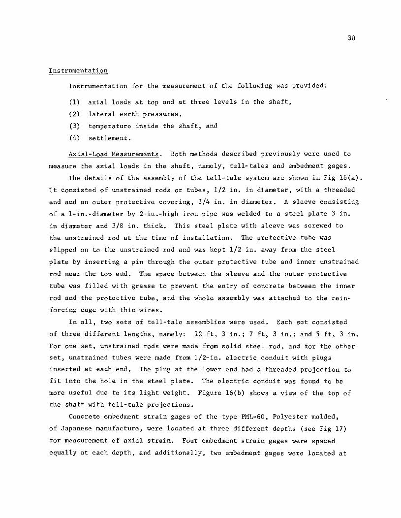
Instrumentation for the measurement of the following was provided:

(1) axial loads at top and at three levels in the shaft,

(2) lateral earth pressures,

(3) temperature inside the shaft, and

(4) settlement.

30

Axial-Load Measurements. Both methods described previously were used to

measure the axial loads in the shaft, namely, tell-tales and embedment gages.

The details of the assembly of the tell-tale system are shown in Fig l6(a).

It consisted of unstrained rods or tubes, 1/2 in. in diameter, with a threaded

end and an outer protective covering, 3/4 in. in diameter. A sleeve consisting

of a l-in.-diameter by 2-in.-high iron pipe was welded to a steel plate 3 in.

in diameter and 3/8 in. thick. This steel plate with sleeve was screwed to

the unstrained rod at the time of installation. The protective tube was

slipped on to the unstrained rod and was kept 1/2 in. away from the steel

plate by inserting a pin through the outer protective tube and inner unstrained

rod near the top end. The space between the sleeve and the outer protective

tube was filled with grease to prevent the entry of concrete between the inner

rod and the protective tube, and the whole assembly was attached to the rein­

forcing cage with thin wires.

In all, two sets of tell-tale assemblies were used. Each set consisted

of three different lengths, namely: 12 ft, 3 in.; 7 ft, 3 in.; and 5 ft, 3 in.

For one set, unstrained rods were made from solid steel rod, and for the other

set, unstrained tubes were made from 1/2-in. electric conduit with plugs

inserted at each end. The plug at the lower end had a threaded projection to

fit into the hole in the steel plate. The electric conduit was found to be

more useful due to its light weight. Figure l6(b) shows a view of the top of

the shaft with tell-tale projections.

Concrete embedment strain gages of the type PML-60, Polyester molded,

of Japanese manufacture, were located at three different depths (see Fig 17)

for measurement of axial strain. Four embedment strain gages were spaced

equally at each depth, and additionally, two embedment gages were located at

,0001- in Dial Indicator

Unstrained Tube

Space Filled With Oil

Protective Outer Coverinc;l

.. . ; .<~.': ...

Space Filled With Grease

I-in-dia x 2-in Iron Pipe Sleeve

3 - in- dia K 3/8 -in

Steel Plate

,,' f '

.. > , " " .".. . ... " ..

'~::i ~'. I ~:,'$,'" ... " .... ,. ... '. '.... ). . .... . ... ' . . ',. ' .. :: ~ .

Left -Hand-Threaded End

Thread Hole to Fit

Fig 16(a). Details of the assembly of the tell-tale system.

31

--

32

Fig l6(b). View of tell-tales at top of shaft.

a depth of 6.8 ft to measure lateral strain. At each location one of the

gages was placed in a concrete block of 3 X 7 X 1 in.

33

All embedment gages were used as a single active element in a Wheat­

stone bridge circuit. The "dununy" gage used was cast in a concrete cylinder

and buried 6 ft in the soil near the test shaft. This dununy was used in the

bridge circuit as the adjacent arm for temperature compensation.

A manual balance strain indicator was used for readout of all measuring

circuits completed through a pair of ten-channel "switch and balance" units.

Electrical connections between the readout equipment and the embedment

gages were made through four conductor, shielded cables of Belden type 8723.

Each cable carried connections to two gages. The solder connections between

the cable and gage leads were protected with ''heat shrinkable" tubing and

coated with rubber to metal cement.

This method of waterproofing was found to be inadequate and a possible

contribution to the low electrical leakage resistance encountered after a

period of several weeks.

Location of the "dummy" strain gage in an "unstrained" environment

within the shaft would also provide better temperature compensation for

measuring circuits.

Lateral-Earth-Pressure Measurements. Details of the diaphragm-type

pressure cells used to measure lateral earth pressure and the method of

installation are described in a separate report, and only a brief descrip­

tion of the cells is given here. The locations of these cells are shown in

Fig 17.

The lateral-earth-pressure cells were developed by project personnel at

The University of Texas for use on this project. The cells were machined from

a berillium-copper alloy to provide a thin diaphragm sensing area. This

sensing area was instrumented with Baldwin Lima Hamilton type FAES-4-150-1256,

four arm, foil strain gages.

The full bridge configuration of this strain gage provided the necessary

sensitivity and temperature compensation for use as a pressure transducer.

The sealed transducer was provided with a copper-tubing fitting to accept

the tubing for lead-wire protection to the surface. These gages were moni­

tored with a manual balancing strain indicator through a special switch and

balance unit which provided indicator zero and calibration check facility.

Number 2 4 6

f- r-- r--

16 in

L

2ft --

4ft --

6ft --

8ft --

o B

H

0 0 3

3 ~I I = - 3.5ft

C

G

I t:. 2

5.4 ft

0 6.0ft 4

p~

c::::J H 6.8ft

I 2 lOft -- 0 o IO.Oft

i~D I A I

IO.4ft

L K

12ft --

1..-24in-.l

o South

Reaction

Legend:

Jh =

0 =

I = - = r:::::::l =

0 = .6. =

A 6

Tell~Tales

o North

Reaction

Embedment Gagel Precast in Mortar Block Placed Vertically

Embedment Gages Placed Vertically

Embedment Gages Placed Horizontally

Embedment Gagel Precast in Mortar Block Placed Horizontally

~ateral Pressure Gages

Ther mo Cou pies

Fig 17. Locations of strain gages, tell-tales, lateral pressure gages, and thermocouples.

34

35

Temperature and Moisture Measurements. Thermocouples were installed in

the test shaft to monitor the temperature variation. The locations of these

are shown in Fig 17. The thermocouples were monitored with a Leeds and Nor­

throp portable potentiometer.

Moisture measurements were taken from the soil samples obtained at the

site location before test shaft installation. It was planned that a regular

monitor of moisture be kept by using a "nuclear moisture" probe; however,

due to a long delay in purchase and calibration of a "down hole" probe this

device was not ready for use during the the testing at this site.

Loading Equipment

The head of the concrete shaft was capped with molding plaster in a

manner to produce a horizontal plane bearing surface. A 1/2-in.-thick

circular steel plate 24 in. in diameter was put on top of the shaft cap.

This steel plate had six holes, each 1-1/2 in. in diameter, at locations

corresponding to the tell-tale projections above the shaft head. A loading

head (Fig 18) was used to transfer the load from the bottom of the jack to

the top of the steel plate.

A jack of 400-ton capacity was used. Half-inch-thick plywood was put at

the top of the hydraulic ram to provide uniform contact. Steel spacer

plates of I-in. thickness were also used between the plywood and the box

that was fixed across the reaction beams. Reaction beams consisted of two

36 WF sections.

Load Tests

In all, eight axial-load tests were carried out at this site. The date

of testing and type of tests were as shown in Table 1.

Tests 1 through 3 were conducted to evolve a suitable loading procedure

and to determine the reliability and repeatability of the instrumentation

used in the shaft. The load was applied in 10-ton increments and held for

30 min. During that time readings were taken for all shaft instrumentation

at intervals of 1/2, 4, 8, 15, and 25 min for each loading increment. On

completion of readings for a 40-ton load, the shaft was unloaded immediately

to a zero load, and additional readings were then made for a period of 30

min.

Fig 18. View of loading head, settlement gages, and tell tales.

36

37

TABLE 1. SCHEDULE OF TESTING

Test Incremental Maximum Load No. Date Time, min Applied, tons

1 Oct. S, 1966 30.0 40

2 Oct. 19, 1966 30.0 40

3 Oct. 21, 1966 30.0 40

4 Feb. 2, 1967 30.0 20

S Feb. 3, 1967 30.0 160

6 Mar. lS, 1967 lS.O 160

7 Mar. 22, 1967 2.S lSO

8 Mar. 22, 1967 2.S lSO

Test 4 was carried out a day before the full-scale load test to check

out the instrumentation. Tests Sand 6 were full-scale load tests. The

failure load, found to be 160 tons, here refers to the ultimate load at

which the hydraulic loading jack had to be pumped continuously to maintain

the load. The loading procedure was essentially the same as in earlier tests

except that the time interval between two loadings was lS min for Test 6.

Tests 7 and 8 were run according to the "Quick Test Load Method" of the

Texas Highway Department. Test 8 was started one hour after the unloading

for Test 7.

The load-settlement curves for Tests S through 8 are shown in Fig 19.

Discussion of Results

Since this test shaft was primarily meant to develop suitable instru­

mentation, test procedure, and related features, the data were not analyzed

rigorously. However, the results of Tests 6, 7, and 8 were very similar.

A typical load distribution in the shaft is shown in Fig 20. The load trans­

ferred to the tip of the shaft was about 18 to 30 percent of the failure load

applied at the top.

Temperature variation created considerable drift in the strain gage

readings, but it is felt that the provision of one dummy strain gage at

each location of active strain gages will reduce this drift. Further,

equal spacing of strain gages at each location should red~ce the effect of

eccentricity in loading.

., II Jt:. U c:

0.5

1.0

.. 1.5 .. c: II e II ;: .. II (I)

• ~ 2.0 to.

C>

2.5

o Load on Top of Shaft, tons

40 80 120 160

• ___ ~--l7-fl-6-~ __ ~

Test No.5 Feb 3, 1967

Test NO.6

~R:.o.nd · \ · yM" 15, '.6'

0-0-0--0-0--0-0:-0_

Rebound "

I~~Q-~~O:-::O:-~O-~2:~::~~::::::~~ ~ 0-0__ ~T.st No.7 3.0 Rebound 00-0 Mar 22, 1967

" CJ

~Rebound -a~ Teit No.8 Mar 22, 1967

3.5

Fig 19. Load-settlement curves at Montopo1is site.

38

.. .... .. .... 1:1 .I:: (I)

.... 0 a. 0 I-JI 0 ...

CXI

.I:: .. a. II)

Q

Loa d in t he Shaft, tons

o 40 80 120 160 0~~----------+----------~----------+----------4~

6

8

10

12

14

16

18

20

Fig 20. Typical load-distribution curves for Test 7 at Montopolis site.

39

CHAPrER 6. PRELIMINARY METHOD FOR COMPUTING ULTIMATE CAPACITY OF A DRILLED SHAFT

The aim of the research reported herein is to develop methods for

computing the behavior of drilled shafts in a wide variety of soils and for

various environmental conditions. This goal cannot be realized until a

considerable amount of data is obtained to provide reasonable predictions

of load-transfer curves for the sides of the shaft and of a load-settlement

curve for the tip of the shaft.

However, a preliminary method of computing the ultimate capacity of a

drilled shaft should be useful as an interim guide. The method can be ex­

panded and improved as results of tests become available. The weakness of

this preliminary method is, of course, that the settlement corresponding to

the ultimate capacity is unknown. Further, the method is based only on the

preliminary results in this report and is limited to soil types similar to

those at the Montopolis site.

The computation of the ultimate load on a drilled shaft proceeds in two

parts: computation of load carried (1) by the side of the drilled shaft

and (2) by the tip of the drilled shaft. This method assumes no interaction

between the tip and the sides of the shaft in carrying load, an assumption

which is not strictly correct but is sufficiently valid for the present

purposes. Future research in this project will consider this interaction.

Computing Load Capacity Along the Side of a Drilled Shaft

The load carried by the side of the drilled shaft can be estimated by

using the modified shearing resistance of the soil. The procedure involves

dividing the shaft into a number of increments, calculating the load capacity

for each increment, and summing this load. Specifically, the procedure is

as follows:

(1) Using the modified shearing resistance of the soil, compute the load carried by each increment along the drilled shaft by usi r

the following expression:

40

where

41

t.R. M.c.a. ~ ~ ~

(13) ~

M.

ct. ~

c. ~

~

shaft side resistance at the ith increment,

area of the side ~~ the drilled shaft in contact with the soil at the i increment,

h · 1 f h .th. t e m~nimum va ue 0 a at t e ~ ~ncrement,

shearing resistance of an undisturbed sample at the ith increment.

(2) The estimated load carried by the side of the drilled shaft is equal to the sum of the shaft side resistance of each increment. Thus,

R M

·L:1t.R· ~= ~

M ·L:1/SA·c.a. ~= ~ ~ ~

where M is the total number of increments.

(14)

The Montopo1is shaft, 2 ft in diameter and 12 ft long, is used in the

following example of this procedure. The moisture content and unconfined

compression strength variations are shown in Fig 21 where Curve A is the

best second degree least squares fit to twelve feet for moisture content,

and Curve B is the best fit for unconfined compression strength. The water­

cement ratio of the concrete was 0.6.

Undisturbed samples were tested for moisture migration at depths of 3,

6, 8, 9, 11, and 13 ft. The overburden pressure applied during the curing

periods for samples at 8, 9, 11, and 13 ft was 10 psi, while an overburden

pressure of 5 psi was used for the samples taken at 3 and 6 ft. These over­

burden pressure values were taken to represent the approximate lateral pres­

sures exerted by the concrete on the soil at the various levels as computed

by the ACI formula for lateral concrete pressure on form work (Ref 6). Actual

lateral pressure variations will be discussed in a later report. The moisture

content versus distance from the interface at each depth obtained from these

tests is shown in Fig 22, and the average moisture-content increase in the

first inch for various water-cement ratios is given in Table 2. Moisture

migrated up to 1-1/2 in. into the soil, thus decreasing the shear strength

in that region near the interface.

2

4

6

8

.... .... .. 10

.t:. .... Q. t)

o 12

14

16

18

20

Orilled

Shaft

CL)

10

a

Curve A

Moisture Content, 0/0

15 20

'I x I I .,

I I I I , ,

25

~ Estimated Moisture It After Fresh Concrete

Is Poured a Original Moisture

aContent

o

42

Curve B

Unconfined Compression

I o I

I , o I

I I J 10 ,

I

5

I 0

I ,0 I I I

o

o

o

Strength, tsf

o

10

o o

15

Unconfined Compression Strength

Estimated Unconfined Compression Strength After Fresh Concrete Is Poured

,Fig 21. Estimated moisture and shearing resistance of soil at various depths.

Depth in feet

6

~ 0 ~

8 -c: ., -c: 0 u ., ...

:::J -It '0

9 2

II

13

Distance from Interface, inches

0 1.0 2.0 3.0 4.0

24

22 - - - - - - ___ - - - -0

20

20

18 -------------0 16 19

17

--- ----------0 15 18 •

16 ........

14 16

.... -.... --- ....... ----0

14 ------------0 12 18

16 ------------~

14

Fig 22. Variation in moisture content with distance from interface.

43

44

TABLE 2. MOISTURE MIGRATION ON UNDISTURBED SAMPLES

Water-Cement Water-Cement Water-Cement Ratio 0.6 Ratio := 0.7 Ratio := 0.8

Depth ft

Initial b.w Average Initial b.w Average Initial b.w Average Moisture Increase in Moisture Increase in Moisture Increase in Content First Inch Content First Inch Content First Inch

3 27.10 23.15 0.44 21.60 1.30

6 18.00 0.37 17 .28 2.23 18.35 2.60

8 16.00 1.61 16.10 2.24 16.00 3.28

9 13.70 3.19 13.10 3.42 13.70 4.88

11 13 .82 2.08 13 .82 2.04 13.80 2.33

13 15.00 1. 99 14.30 2.38 14.95 3.24

15 12.70

Direct shear tests to study the shearing plane developed at various

distances from the interface were conducted on mortar-soil samples taken

from the same depths and tested at the same overburden pressures (the 3-ft

sample was omitted). The results of these tests are plotted in Fig 23.

Figure 23 clearly indicates that the zone of weakest soil occurs at

about 1/4 in. from the interface. Hence, the soil in this zone will have

its maximum shearing resistance mobilized first, and failure will occur at

approximately 1/4 in. from the interface.

Assuming the shearing resistance of the soil is fully developed along

the drilled shaft, the total load on the side of the drilled shaft is equal

to R. The computation of the load is shown in Table 3, with the computed

load being 104.5 tons.

The actual side load obtained from analyzing the results of Test 6 was

106 tons. The side load was separated from the total load applied at the

top of t~e shaft by the use of instrumentation along the shaft. For this

test, the agreement between computed and experimental values of the side

load was very good.

Depth in feet

0.9 a

6 0.7

0.5

0.9

a 8 0.7

0.5 0.9

Q

9 0.7

0.5

0.9

II 0.7 Q

0.5

0.9 a

13 0.7

0.5

o Distance from Interface, inches

1.0 I

2.0 3.0

\.-----' II

II

'\ II

\ ll, II

II

\ II

\ II

II

\,.

Fig 23. Variation in a with distance from interface.

45

46

TABLE 3. LOAD COMPUTATION

Depth Interval c Ci c Ci M. ~

ft TSF TSF ft2 tons

0-6 1. 70 0.79 1.34 38.46 51.5

6-8 2.10 0.52 1.09 12.82 15.6

8-9 2.55 0.53 1.35 6.44 7.8

9-11 3.48 0.50 1. 74 12.82 19.9

11-12 2.50 0.51 1.28 6.44 9.7

Total load carried by side of the drilled shaft 104.5

If no reduction is made for loss in shear strength due to moisture

migration, the computed capacity of the side of the drilled shaft is 189 tons.

Considering moisture migration, however, the capacity is 104.5 tons. Thus,

it is important to take into account the moisture migration and consequent

strength loss.

Computing Load Capacity at the Tip of a Drilled Shaft

The load capacity of the tip of a drilled shaft can be computed by use

of bearing-capacity theory. Assuming the unit weight of concrete is the same

as the unit weight of soil, the following equation can be used to compute the

load capacity of the tip:

(15)

where

QB

ultimate tip load,

N bearing-capacity factor at the tip of the shaft, c

~ area of the tip of the shaft,

modified shearing strength of soil at the tip of the shaft.

47

Formulas for the bearing-capacity factors have been presented by a

number of authors. The method proposed by Skempton (Ref 5) is well accepted

for clay soils at the present time. For a circular footing, Skempton's

recommendations for N are shown in Fig 24. c

Perhaps the most difficult problem in determining the ultimate bearing

capacity of the tip of the drilled shaft is ascertaining the soil shear

strength. While it is known that some softening will occur, the amount of

moisture migration and shear strength loss is unknown at present.

In this analysis it is assumed that the modified shear strength is midway

between the initial shear strength and the fully softened shear strength; thus,

a value of 1.88 TSF will be employed (see Table 3). Substituting into Eq 15

QB (9)(n)(1.88)

53 tons •

The bearing-capacity factor N c

9 is estimated from Fig 24.

The measured load carried by the tip of the shaft was 54 tons, as

(16)

determined from results of Test 6. This value agrees extremely well with the

computed tip load of 53 tons.

Actually, the moisture content of the soil around the drilled shaft

changes with time, that is, with periods of heavy and prolonged rainfall or

periods of severe drought. As a consequence, changes in the soil properties

and in the load transfer characteristics will occur. Therefore, the computa­

tions shown are valid only for a certain period of time after the shaft has

been constructed. The nature of the adjustments that will have to be made in

computation procedures to account for future precipitation variations is at

present unknown.

10

9

8

7

u z

6 ... 0 .. u 0

I.L.

>. 5

V /' ..

u 0 0. 0 0 4 01 .: ... 0 4D ID 3

2

o o

j j

~ ~

C;"",\' Square ~ --~

StriP"""\..

~ ----0 B

0.0

0.25

0.5

0.75

1.0

1.5

2.0

2.5

3.0

4.0

>4.0

~No Strip

6.2

6.7

7.1

7.4

7.7

8.1

8.4

8.6

8.8

9.0

9.0

5.14

5.6

5.9

6.2

6.4

6.8

7.0

7.2

7.4

7.5

7.5

2 3 D :: Depth To Foundation B Breadth of Foundation

y T -

"'l [\'\\\\\\\' ",'."" .. , Cl f

..............,

D

L -

~ ~ B - -xL

Nc(rec) :: [0.84 +0.16 ~ ] Nc (sq) -Clf :: cNc .. P

c :: Shear Strength

P = Overburden Pressure -

At Foundation Level

I I I 4 5

Fig 24. Bearing capacity factors for foundations in clay (¢ 0) ( fr om Re f 5).

CHAPTER 7. SUMMARY AND RECOMMENDATIONS

The problems of designing drilled shafts are complex, involving a

variety of factors with a spatial and time variability. Accurate determina­

tion of the load-carrying capacity of drilled shafts is practically impos­

sible because so many effects are not well defined. In particular, the

load-settlement and the load-distribution curves for shafts cannot be easily

determined. Superposed on the requirements for a particular shaft are the

wide variety of soil and environmental conditions in which such shafts must

be constructed.

The physical requirements and the testing program described herein are

vital to the development of a rational procedure for designing drilled shafts.

This is the first in a series of reports planned to describe the important

parts of the program. The others include:

(1) a report describing the development of instrumentation and the study of lateral earth pressure against shafts,

(2) a study and report on the soils aspects of the problem, including the problems of soil-concrete interaction and the measurement of shear strength,

(3) a report describing the development of instrumentation for measuring moisture migration near drilled shafts,

(4) reports on a series of load tests on a full-sized shaft in San Antonio, Texas, to develop necessary load-distribution and load­settlement information for a particular location,

(5) reports on a second series of load tests on full-sized shafts in Houston, Texas, to study the same factors under different soils and environmental conditions,

(6) reports on an effort to combine all data developed in Items 1 through 5 into a preliminary design approach for drilled shafts considering as many factors as realistically possible, and

(7) a study of the problem in the light of the preliminary design approach to see what future investigations are desirable and how sensitive the proposed method is to various other factors.

It has been the purpose of this report to put the problems of designing

drilled shafts in perspective and to develop the preliminary procedures which

49

50

will be used in subsequent phases. Several other reports will be forthcoming

in the very near future as testing and analysis are completed.

REFERENCES

1. Reese, Lymon C., "Load Versus Settlement for an Axially Loaded Pile," Proceedings, Symposium on Bearing Capacity of Piles, Part 2, Central Building Research Institute, Roorkee, February 1964, pp. 18-38.

2. Seed, H. B. and Lymon C. Reese, "The Action of Soft Clay Along Friction Piles," Transactions, American Society of Civil Engineers, Vol 122, 1957, pp 731-764.

3. Coyle, Harry M. and Lymon C. Reese, "Load Transfer for Axially Loaded Piles in Clay," Journal of the Soil Mec;hanics and Foundations Division, American Society of Civil Engineers, Vol 92, No SM2, March 1966, pp 1-26.

4. Coyle, Harry M. and Ibrahim H. Sulaiman, "Skin Friction for Steel Pipes in Sand,1I Proceedings, American Society of Civil Engineers, Vol 93, No SM6, November 1967, pp 261-278.

5. Skempton, A. W., "The Bearing Capacity of Clays," Building Research Congress, Division I, Part III, 1951, pp 180-189.

6. "Recommended Practices for Concrete Formwork," Standards, American Concrete Institute, 1963, pp 347 - 363.

51