153
Fifth International Workshop on Formal Techniques for Safety-Critical Systems (FTSCS 2016) Preliminary Proceedings Editors: Cyrille Artho and Peter Csaba ¨ Olveczky
| Date post: | 08-May-2018 |
| Category: |
Documents |
| Upload: | trinhkhuong |
| View: | 217 times |
| Download: | 0 times |
Fifth International Workshop on
Formal Techniques for Safety-Critical Systems
(FTSCS 2016)
Preliminary Proceedings
Editors: Cyrille Artho and Peter Csaba Olveczky
Preface
This volume contains the preliminary proceedings of the Fifth InternationalWorkshop on Formal Techniques for Safety-Critical Systems (FTSCS 2016),held in Tokyo November 14, 2016, as a satellite event of the ICFEM conference.
The aim of this workshop is to bring together researchers and engineers whoare interested in the application of formal and semi-formal methods to improvethe quality of safety-critical computer systems. FTSCS strives to promote re-search and development of formal methods and tools for industrial applications,and is particularly interested in industrial applications of formal methods. Spe-cific topics include, but are not limited to:
• case studies and experience reports on the use of formal methods foranalyzing safety-critical systems, including avionics, automotive, railway,medical, and other kinds of safety-critical and QoS-critical systems;
• methods, techniques and tools to support automated analysis, certifica-tion, debugging, etc., of complex safety/QoS-critical systems;
• analysis methods that address the limitations of formal methods in indus-try (usability, scalability, etc.);
• formal analysis support for modeling languages used in industry, such asAADL, Ptolemy, SysML, SCADE, Modelica, etc.; and
• code generation from validated models.
The workshop received 23 regular paper submissions. Each submission wasreviewed by at least three referees. Based on the reviews and extensive discus-sions, the program committee selected 9 papers for presentation at the workshopand inclusion in this volume. Another highlight of the workshop is an invitedtalk by Naoki Kobayashi.
Revised versions of accepted papers will appear in the post-proceedings ofFTSCS 2016 that will be published as a volume in Springer’s Communications inComputer and Information Science (CCIS) series. Extended versions of selectedpapers from the workshop will also appear in a special issue of the Science ofComputer Programming journal.
Many colleagues and friends have contributed to FTSCS 2016. We thankNaoki Kobayashi for accepting our invitation to give an invited talk and theauthors who submitted their work to FTSCS 2016 and who, through their con-tributions, make this workshop an interesting event. We are particularly gratefulthat so many well known researchers agreed to serve on the program committee,and that they provided timely, insightful, and detailed reviews. We also thankthe editors of Communications in Computer and Information Science for agree-ing to publish the proceedings of FTSCS 2016 as a volume in their series, andShaoying Liu and Shin Nakajima for their help with the local arrangements.
We hope that you will all enjoy the workshop!
November, 2016 Cyrille ArthoPeter Csaba Olveczky
I
Program Chairs
Cyrille Artho KTH Royal Institute of Technology
Peter Csaba Olveczky University of Oslo
Program Committee
Etienne Andre University Paris 13Toshiaki Aoki JAISTCyrille Artho KTH Royal Institute of TechnologyKyungmin Bae Pohang University of Science and TechnologyEun-Hye Choi AISTAlessandro Fantechi University of Florence and ISTI-CNR, PisaBernd Fischer Stellenbosch UniversityOsman Hasan National University of Sciences & TechnologyKlaus Havelund NASA JPLJerome Hugues Institute for Space and Aeronautics EngineeringMarieke Huisman University of TwenteRalf Huuck SynopsysFuyuki Ishikawa National Institute of InformaticsTakashi Kitamura AISTAlexander Knapp Augsburg UniversityThierry Lecomte ClearSy System EngineeringYang Liu Nanyang Technological UniversityRobi Malik University of WaikatoFrederic Mallet Universite Nice Sophia AntipolisRoberto Nardone University of Napoli “Federico II”Vivek Nigam Federal University of ParaıbaThomas Noll RWTH Aachen UniversityKazuhiro Ogata JAIST
Peter Csaba Olveczky University of OsloCharles Pecheur Universite catholique de LouvainMarkus Roggenbach Swansea UniversityRalf Sasse ETH ZurichMartina Seidl Johannes Kepler University LinzOleg Sokolsky University of PennsylvaniaSofiene Tahar Concordia UniversityCarolyn Talcott SRI InternationalTatsuhiro Tsuchiya Osaka UniversityAndras Voros Budapest University of Technology and EconomicsChen-Wei Wang State University of New York (SUNY)Mike Whalen University of MinnesotaHuibiao Zhu East China Normal University
II

Additional Reviewers
Beillahi, Sidi Mohamed Gillard, XavierBukhari, Syed Ali Asadullah Oortwijn, WytseDu, Xiaoning Qasim, MuhammadFang, Huixing Sardar, Muhammad UsamaGentile, Ugo Van Zijl, Lynette
III
Table of Contents
Invited Talk
On Two Higher-Order Extensions of Model Checking . . . . . . . . . . . . . . . . . . . . . 1
Naoki Kobayashi
Specification and Verification
Specification and Verification of Synchronization with Condition Variables 3
Pedro de Carvalho Gomes, Dilian Gurov and Marieke Huisman
An interval logic for stream-processing functions: A convolution-basedconstruction . . . . . . . . . . . . . . . . . . . . . . . . . . . . . . . . . . . . . . . . . . . . . . . . . . . . . . . . . . . . . . 19
Brijesh Dongol
Automotive and Railway Systems
Automating Time Series Safety Analysis for Automotive ControlSystems in STPA using Weighted Partial Max-SMT. . . . . . . . . . . . . . . . . . . . . . . 35
Shuichi Sato, Shogo Hattori, Hiroyuki Seki, Yutaka Inamori and ShojiYuen
Uniform Modeling of Railway Operations . . . . . . . . . . . . . . . . . . . . . . . . . . . . . . . . . 51
Eduard Kamburjan and Reiner Hahnle
Security, Internet of things
Formal Verification of Gate-Level Multiple Side Channel Parameters todetect Hardware Trojans. . . . . . . . . . . . . . . . . . . . . . . . . . . . . . . . . . . . . . . . . . . . . . . . . . 68
Imran Abbasi, Faiq Khalid Lodhi, Awais Kamboh and Osman Hasan
Formal Probabilistic Analysis of a WSN-based Monitoring Frameworkfor IoT Applications . . . . . . . . . . . . . . . . . . . . . . . . . . . . . . . . . . . . . . . . . . . . . . . . . . . . . . 85
Maissa Elleuch, Osman Hasan, Sofiene Tahar and Mohamed Abid
Cyber-Physical Systems and Parameterized Verification
Shared-Variable Concurrency, Continuous Behaviour and Healthiness forCritical Cyberphysical Systems . . . . . . . . . . . . . . . . . . . . . . . . . . . . . . . . . . . . . . . . . . . 101
Richard Banach and Huibiao Zhu
Applying parametric model-checking techniques for reusing real-timecritical systems . . . . . . . . . . . . . . . . . . . . . . . . . . . . . . . . . . . . . . . . . . . . . . . . . . . . . . . . . . . 117
Baptiste Parquier, Laurent Rioux, Rafik Henia, Romain Soulat,
Olivier H. Roux, Didier Lime and Etienne Andre
Parameterised Verification of Stabilisation Properties via ConditionalSpotlight Abstraction . . . . . . . . . . . . . . . . . . . . . . . . . . . . . . . . . . . . . . . . . . . . . . . . . . . . . 133
Nils Timm and Stefan Gruner
IV
On Two Higher-Order Extensions ofModel Checking
Naoki Kobayashi
The University of [email protected]
Inspired by the success of finite state model checking [1] in system verification,two kinds of its higher-order extensions have been studied since around 2000.One is model checking of higher-order recursion schemes (HORS) [2, 10], wherethe language for describing systems to be verified is extended to higher-order,and the other is higher-order fixpoint modal logic (HFL) model checking offinite-state systems [14], where the logic for specifying properties to be verified isextended to higher-order. The former has been successfully applied to automatedverification of higher-order programs [3, 4, 6–8, 11–13, 15], whereas the latter hasbeen studied for verification of concurrent systems [9, 14]. In the talk, I willprovide a gentle introduction to the HORS and HFL model checking problems,their applications to software verification, and the state-of-the-art of higher-ordermodel checkers and tools built on top of them. I will also touch upon our recentresult on the relationship between HORS and HFL model checking [5].
References
1. Clarke, E.M., Grumberg, O., Peled, D.A.: Model Checking. The MIT Press (1999)2. Knapik, T., Niwinski, D., Urzyczyn, P.: Higher-order pushdown trees are easy. In:
FoSSaCS 2002. LNCS, vol. 2303, pp. 205–222. Springer (2002)3. Kobayashi, N.: Types and higher-order recursion schemes for verification of higher-
order programs. In: Proc. of POPL. pp. 416–428. ACM Press (2009)4. Kobayashi, N.: Model checking higher-order programs. Journal of the ACM 60(3)
(2013)5. Kobayashi, N., Etienne Lozes, Bruse, F.: On the relationship between higher-order
recursion schemes and higher-order modal fixpoint logic. In: Proceedings of POPL2017 (2017), to appear
6. Kobayashi, N., Sato, R., Unno, H.: Predicate abstraction and CEGAR for higher-order model checking. In: Proc. of PLDI. pp. 222–233. ACM Press (2011)
7. Kobayashi, N., Tabuchi, N., Unno, H.: Higher-order multi-parameter tree trans-ducers and recursion schemes for program verification. In: Proc. of POPL. pp.495–508. ACM Press (2010)
8. Kuwahara, T., Sato, R., Unno, H., Kobayashi, N.: Predicate abstraction and CE-GAR for disproving termination of higher-order functional programs. In: Proceed-ings of CAV 2015. Lecture Notes in Computer Science, vol. 9207, pp. 287–303.Springer (2015)
9. Lange, M., Lozes, E., Guzman, M.V.: Model-checking process equivalences. Theor.Comput. Sci. 560, 326–347 (2014)
10. Ong, C.H.L.: On model-checking trees generated by higher-order recursionschemes. In: LICS 2006. pp. 81–90. IEEE Computer Society Press (2006)
1
11. Ong, C.H.L., Ramsay, S.: Verifying higher-order programs with pattern-matchingalgebraic data types. In: Proc. of POPL. pp. 587–598. ACM Press (2011)
12. Sato, R., Unno, H., Kobayashi, N.: Towards a scalable software model checkerfor higher-order programs. In: Proceedings of PEPM 2013. pp. 53–62. ACM Press(2013)
13. Unno, H., Terauchi, T., Kobayashi, N.: Automating relatively complete verifica-tion of higher-order functional programs. In: The 40th Annual ACM SIGPLAN-SIGACT Symposium on Principles of Programming Languages, POPL 2013. pp.75–86. ACM (2013)
14. Viswanathan, M., Viswanathan, R.: A higher order modal fixed point logic. In:CONCUR. Lecture Notes in Computer Science, vol. 3170, pp. 512–528 (2004)
15. Watanabe, K., Sato, R., Tsukada, T., Kobayashi, N.: Automatically disproving fairtermination of higher-order functional programs. In: Proceedings of ICFP 2016. pp.243–255. ACM (2016)
2
Specification and Verification of Synchronizationwith Condition Variables
Pedro de Carvalho Gomes1, Dilian Gurov1, and Marieke Huisman?2
1 KTH Royal Institute of Technology, Stockholm, Sweden2 University of Twente, Enschede, The Netherlands
In this paper we propose a technique to specify and verify the correct synchro-nization of concurrent programs with condition variables. We define correctnessas the liveness property: “every thread synchronizing under a set of conditionvariables eventually exits the synchronization”, under the assumption that everysuch thread eventually reaches its synchronization block. Our technique doesnot avoid the combinatorial explosion of interleavings of thread behaviors. In-stead, we alleviate it by abstracting away all details that are irrelevant to thesynchronization behavior of the program, which is typically significantly smallerthan its overall behavior. First, we introduce SyncTask, a simple imperativelanguage to specify parallel computations that synchronize via condition vari-ables. We consider a SyncTask program to have a correct synchronization iffit terminates. Further, to relieve the programmer from the burden of providingspecifications in SyncTask, we introduce an economic annotation scheme for Javaprograms to assist the automated extraction of SyncTask programs capturing thesynchronization behavior of the underlying program. We prove that every Javaprogram annotated according to the scheme (and satisfying the assumption) hasa correct synchronization iff its corresponding SyncTask program terminates. Weshow how to transform the verification of termination into a standard reachabil-ity problem over Colored Petri Nets that is efficiently solvable by existing PetriNet analysis tools. Both the SyncTask program extraction and the generationof Petri Nets are implemented in our STaVe tool. We evaluate the proposedframework on a number of test cases as a proof-of-concept.
1 Introduction
Condition variables (CV) are a commonly used synchronization mechanism tocoordinate multithreaded programs. Threads wait on a CV, meaning they sus-pend their execution until another thread notifies the CV, causing the waitingthreads to resume their execution. The signaling is asynchronous: if no threadis waiting on the CV, then the notification has no effect. CVs are used in con-junction with locks; a thread must acquire the associated lock for notifying orwaiting on a CV, and if notified, must reacquire the lock.
Many widely used programming languages feature condition variables. InJava, for instance, they are provided both natively as an object’s monitor [6],i.e., a pair of a lock and a CV, and in the concurrent API, as one-to-many? Supported by ERC grant 258405 for the VerCors project.
3
2 Pedro de Carvalho Gomes, Dilian Gurov, and Marieke Huisman
Condition objects associated to a Lock object. The mechanism is typically em-ployed when the progress of threads depends on the state of a shared variable,to avoid busy-wait loops that poll the state of this shared variable. Nevertheless,condition variables have not been addressed sufficiently with formal techniques,mainly because of the complexity of reasoning about asynchronous signaling. Forinstance, Leino et al. [14] acknowledge that verifying the absence of deadlockswhen using CVs is hard because a notification is “lost” if no thread is waitingon it. Thus, one cannot verify locally whether a waiting thread will eventu-ally be notified. Furthermore, the synchronization conditions can be quite com-plex, involving both control-flow and data-flow aspects as arising from methodcalls; their correctness thus depends on the global thread composition, i.e., thetype and number of parallel threads. All these complexities suggest the need forprogrammer-provided annotations to assist the automated analysis, which is theapproach we are following here.
In this work, we present a formal technique for specifying and verifying that“every thread synchronizing under a set of condition variables eventually exitsthe synchronization”, under the assumption that every such thread eventuallyreaches its synchronization block. The assumption itself is not addressed here, asit does not pertain to correctness of the synchronization, and there already existtechniques for dealing with such properties (see e.g. [16]). Note that the abovecorrectness notion applies to a one-time synchronization on a condition variableonly; generalizing the notion to repeated synchronizations is left for future work.To the best of our knowledge, the present work is the first to address a livenessproperty involving CVs. As the verification of such properties is undecidable ingeneral, we limit our technique to programs with bounded data domains andnumbers of threads. Still, the verification problem is subject to a combinato-rial explosion of thread interleavings. Our technique alleviates the state spaceexplosion problem by delimiting the relevant aspects of the synchronization.
First, we consider correctness of synchronization in the context of a synchro-nization specification language. As we target arbitrary programming languagesthat feature locks and condition variables, we do not base our approach on asubset of an existing language, but instead introduce SyncTask, a simple con-current programming language where all computations occur inside synchronizedcode blocks. We define a SyncTask program to have a correct synchronizationiff it terminates. The SyncTask language has been designed to capture commonpatterns of CV usage, while abstracting away from irrelevant details. SyncTaskhas a Java-like syntax and semantics, and features the relevant constructs forsynchronization, such as locks, CVs, conditional statements, and arithmetic op-erations. However, it is non-procedural, data types are bounded, and it doesnot allow dynamic thread creation. These restrictions render the state-space ofSyncTask programs finite, and make the termination problem decidable.
Next, we address the problem of verifying the correct usage of CVs in realconcurrent programming languages by showing how SyncTask can be used tocapture the synchronization of a Java program, provided it is bounded. There is aconsensus in Software Engineering that synchronization in a concurrent program
4
Specification and Verification of Synchronization with CVs 3
must be kept to a minimum, both in the number and complexity of the synchro-nization actions, and in the number of places where it occurs. This avoids thelatency of blocking threads, and minimizes the risk of errors, such as dead- andlivelocks. As a consequence, many programs present a finite (though arbitrarilylarge) synchronization behavior. To assist the automated extraction of finite syn-chronization behavior from Java programs as SyncTask programs, we introducean annotation scheme, which requires the user to (correctly) annotate, amongothers, the initialization of new threads (i.e., creation of Thread objects), andprovide the initial state of the variables accessed inside the synchronized blocks.We establish that for correctly annotated, bounded Java programs, correctness ofsynchronization is equivalent to termination of the extracted SyncTask program.
As a proof-of-concept of the algorithmic solvability of the termination prob-lem for SyncTask programs, we show how to transform it into a reachability prob-lem on hierarchical Colored Petri Nets3 (CPNs) [7]. We define how to extractCPNs automatically from SyncTask programs, following a previous techniquefrom Westergaard [18]. Then, we establish that a SyncTask program terminatesif and only if the extracted CPN always reaches dead markings (i.e., CPN con-figurations without successors) where the tokens representing the threads arein a unique end place. Standard CPN analysis tools can efficiently compute thereachability graphs, and check whether the termination condition holds. Also,in case that the condition does not hold, an inspection of the reachability grapheasily provides the cause of non-termination.
We implement the extraction of SyncTask programs from annotated Javaand the translation of SyncTasks to CPNs as the STaVe tool. We evaluate thetool on two test-cases, by generating CPNs from annotated Java programs andanalyzing these with CPN Tools [8]. The first test-case evaluates the scalabilityof the tool w.r.t. the size of program code that does not affect the synchronizationbehavior of the program. The second test-case evaluates the scalability of thetool w.r.t. the number of synchronizing threads. The results show the expectedexponential blow-up of the state-space, but we were still able to analyze thesynchronization of several dozens of threads.
In summary, this work makes the following contributions: (i) the SyncTasklanguage to model the synchronization behavior of programs with CVs, (ii) anannotation scheme to aid the extraction of the synchronization behavior of Javaprograms, (iii) an extraction scheme of SyncTask models from annotated Javaprograms, (iv) a reduction of the termination problem for SyncTask programsto a reachability problem on CPNs, (v) an implementation of the framework bymeans of STaVe, and (vi) its experimental evaluation.
The remainder of the paper is organized as follows. Section 2 introducesSyncTask. Section 3 describes the mapping from annotated Java to SyncTask,
3 The choice of formalism has been mainly based on the simplicity of CPNs as ageneral model of concurrency, rather than on the existing support for efficient modelchecking. For the latter, model checking tools exploiting parametricity or symmetriesin the models may prove more efficient in practice.
5
4 Pedro de Carvalho Gomes, Dilian Gurov, and Marieke Huisman
SyncTask ::= ThreadType* MainThreadType ::= Thread ThreadName { SyncBlock* }
Main ::= main { VarDecl* StartThread* }StartThread ::= start(Const,ThreadName);
Expr ::= Const | VarName | Expr � Expr| min(VarName) | max(VarName)
VarDecl ::= VarType VarName(Expr*);VarType ::= Bool | Int | Lock | Cond
SyncBlock ::= synchronized (VarName) Block
Block ::= { Stmt* }Assign ::= VarName = Expr ;
Stmt ::= SyncBlock | Block| Assign | skip;| while Expr Stmt| if Expr Stmt else Stmt| notify(VarName);| notifyAll(VarName);| wait(VarName);
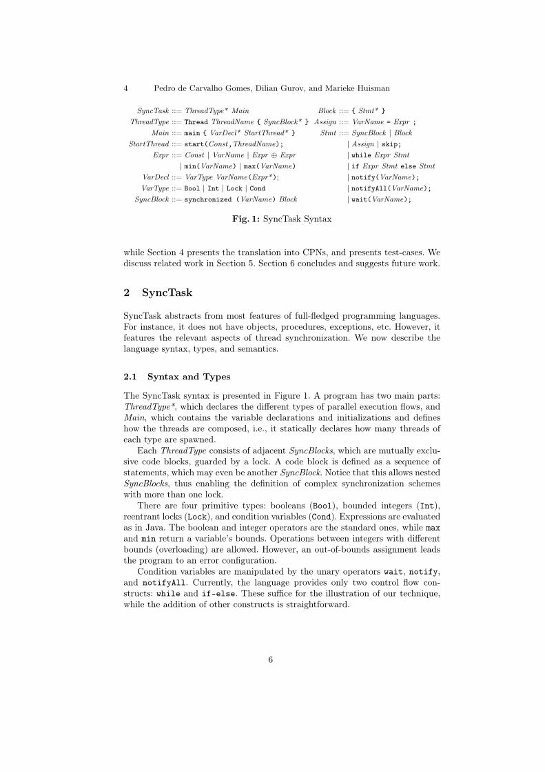
Fig. 1: SyncTask Syntax
while Section 4 presents the translation into CPNs, and presents test-cases. Wediscuss related work in Section 5. Section 6 concludes and suggests future work.
2 SyncTask
SyncTask abstracts from most features of full-fledged programming languages.For instance, it does not have objects, procedures, exceptions, etc. However, itfeatures the relevant aspects of thread synchronization. We now describe thelanguage syntax, types, and semantics.
2.1 Syntax and Types
The SyncTask syntax is presented in Figure 1. A program has two main parts:ThreadType*, which declares the different types of parallel execution flows, andMain, which contains the variable declarations and initializations and defineshow the threads are composed, i.e., it statically declares how many threads ofeach type are spawned.
Each ThreadType consists of adjacent SyncBlocks, which are mutually exclu-sive code blocks, guarded by a lock. A code block is defined as a sequence ofstatements, which may even be another SyncBlock. Notice that this allows nestedSyncBlocks, thus enabling the definition of complex synchronization schemeswith more than one lock.
There are four primitive types: booleans (Bool), bounded integers (Int),reentrant locks (Lock), and condition variables (Cond). Expressions are evaluatedas in Java. The boolean and integer operators are the standard ones, while maxand min return a variable’s bounds. Operations between integers with differentbounds (overloading) are allowed. However, an out-of-bounds assignment leadsthe program to an error configuration.
Condition variables are manipulated by the unary operators wait, notify,and notifyAll. Currently, the language provides only two control flow con-structs: while and if-else. These suffice for the illustration of our technique,while the addition of other constructs is straightforward.
6
Specification and Verification of Synchronization with CVs 5
1 Thread Producer {synchronized(m_lock){
3 while(b_els==max(b_els))wait(m_cond);
5 if(b_els<max(b_els))b_els=(b_els+1);
7 elseskip;
9 notifyAll(m_cond);} }
11 Thread Consumer {synchronized(m_lock){
13 while((b_els==0))wait(m_cond);
15 if((b_els>0))b_els=(b_els-1);
17 elseskip;
19 notifyAll(m_cond);} }
21 main {Lock m_lock();
23 Cond m_cond(m_lock);Int b_els(0,1,1);
25 start(1,Producer);start(2,Consumer);
27 }
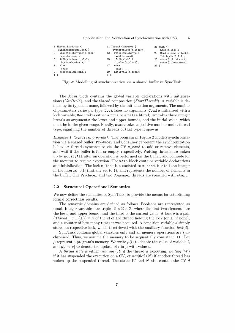
Fig. 2: Modelling of synchronization via a shared buffer in SyncTask
The Main block contains the global variable declarations with initializa-tions (VarDecl* ), and the thread composition (StartThread*). A variable is de-fined by its type and name, followed by the initialization arguments. The numberof parameters varies per type: Lock takes no arguments; Cond is initialized with alock variable; Bool takes either a true or a false literal; Int takes three integerliterals as arguments: the lower and upper bounds, and the initial value, whichmust be in the given range. Finally, start takes a positive number and a threadtype, signifying the number of threads of that type it spawns.
Example 1 (SyncTask program). The program in Figure 2 models synchroniza-tion via a shared buffer. Producer and Consumer represent the synchronizationbehavior: threads synchronize via the CV m_cond to add or remove elements,and wait if the buffer is full or empty, respectively. Waiting threads are wokenup by notifyAll after an operation is performed on the buffer, and compete forthe monitor to resume execution. The main block contains variable declarationsand initialization. The lock m_lock is associated to m_cond. b_els is an integerin the interval [0,1] (initially set to 1), and represents the number of elements inthe buffer. One Producer and two Consumer threads are spawned with start.
2.2 Structural Operational Semantics
We now define the semantics of SyncTask, to provide the means for establishingformal correctness results.
The semantic domains are defined as follows. Booleans are represented asusual. Integer variables are triples Z ⇥ Z ⇥ Z, where the first two elements arethe lower and upper bound, and the third is the current value. A lock o is a pair(Thread_id [ {?}) ⇥ N of the id of the thread holding the lock (or ?, if none),and a counter of how many times it was acquired. A condition variable d simplystores its respective lock, which is retrieved with the auxiliary function lock(d).
SyncTask contains global variables only and all memory operations are syn-chronized. Thus, we assume the memory to be sequentially consistent [11]. Letµ represent a program’s memory. We write µ(l) to denote the value of variable l,and µ[l 7! v] to denote the update of l in µ with value v.
A thread state is either running (R) if the thread is executing, waiting (W )if it has suspended the execution on a CV, or notified (N) if another thread haswoken up the suspended thread. The states W and N also contain the CV d
7
6 Pedro de Carvalho Gomes, Dilian Gurov, and Marieke Huisman
[s1]a T |(✓, synchronized(o) b, R), µ �! T |(✓, synchronized’(o) b, R), µ[o 7! (✓, 1)]
[s2]b T |(✓, synchronized(o) b, R), µ �! T |(✓, synchronized’(o) b, R), µ[o 7! (✓, n + 1)]
[s3]bT |(✓, b1, R), µ �! T |(✓, b2, X), µ0
T |(✓, synchronized’(o) b1, R)), µ �! T |(✓, synchronized’(o) b2, X), µ0
[s4]cT |(✓, b, R), µ �! T |(✓, ✏, R), µ0
T |(✓, synchronized’(o) b, R)), µ �! T |(✓, ✏, R), µ0[o 7! (✓, n � 1)]
[s5]dT |(✓, b, R), µ �! T |(✓, ✏, R), µ0
T |(✓, synchronized’(o) b, R), µ �! T |(✓, ✏, R), µ0[o 7! (?, 0)]
[wt]e T |(✓, wait(d), R), µ ! T |(✓, ✏, (W, d, n)), µ[lock(d) 7! (?, 0)]
[nf1]ef T |(✓, notify(d), R), µ ! T |(✓, ✏, R), µ
[nf2]eg T |(✓, notify(d), R)|(✓0, t0, (W, d, n)), µ ! T |(✓, ✏, R)|(✓0, t0, (N, d, n)), µ
[na1]ef T |(✓, notifyAll(d), R), µ ! T |(✓, ✏, R), µ
[na2]eg T |(✓, notifyAll(d), R)|T dW , µ ! T |(✓, ✏, R)|{(✓0, t0, (N, d, n))|(✓0, t0, (W, d, n)) 2 T d
W }, µ
[rd]h T |(✓, t, (N, d, n)), µ ! T |(✓, t, R), µ[lock(d) 7! (✓, n)]
aµ(o) = (?, 0) bµ(o) = (✓, n) ^ n > 0 cµ(o) = (✓, n) ^ n > 1 dµ(o) = (✓, 1)
eµ(lock(d)) = (✓, n) ^ n > 0 fwaitset(d) = ; gwaitset(d) 6= ; hµ(lock(d)) = (?, 0)
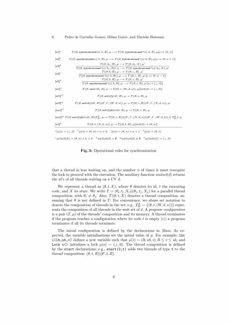
Fig. 3: Operational rules for synchronization
that a thread is/was waiting on, and the number n of times it must reacquirethe lock to proceed with the execution. The auxiliary function waitset(d) returnsthe id’s of all threads waiting on a CV d.
We represent a thread as (✓, t, X), where ✓ denotes its id, t the executingcode, and X its state. We write T = (✓i, ti, Xi)|(✓j , tj , Xj) for a parallel threadcomposition, with ✓i 6= ✓j . Also, T |(✓, t, X) denotes a thread composition, as-suming that ✓ is not defined in T . For convenience, we abuse set notation todenote the composition of threads in the set; e.g., T d
W = {(✓, t, (W, d, n))} repre-sents the composition of all threads in the wait set of d. A program configurationis a pair (T, µ) of the threads’ composition and its memory. A thread terminatesif the program reaches a configuration where its code t is empty (✏); a programterminates if all its threads terminate.
The initial configuration is defined by the declarations in Main. As ex-pected, the variable initializations set the initial value of µ. For example, Inti(lb,ub,v) defines a new variable such that µ(i) = (lb, ub, v), lb v ub, andLock o() initializes a lock µ(o) = (?, 0). The thread composition is definedby the start declarations; e.g., start(2,t) adds two threads of type t to thethread composition: (✓, t, R)|(✓0, t, R).
8
Specification and Verification of Synchronization with CVs 7
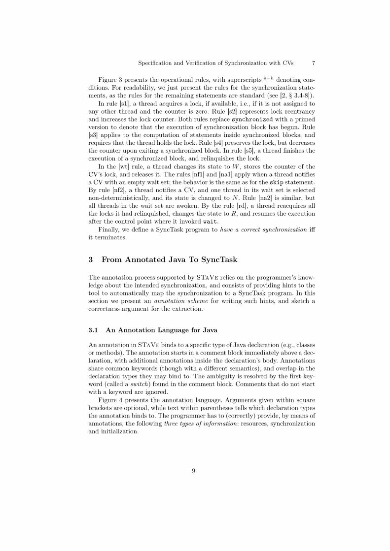
Figure 3 presents the operational rules, with superscripts a�h denoting con-ditions. For readability, we just present the rules for the synchronization state-ments, as the rules for the remaining statements are standard (see [2, § 3.4-8]).
In rule [s1], a thread acquires a lock, if available, i.e., if it is not assigned toany other thread and the counter is zero. Rule [s2] represents lock reentrancyand increases the lock counter. Both rules replace synchronized with a primedversion to denote that the execution of synchronization block has begun. Rule[s3] applies to the computation of statements inside synchronized blocks, andrequires that the thread holds the lock. Rule [s4] preserves the lock, but decreasesthe counter upon exiting a synchronized block. In rule [s5], a thread finishes theexecution of a synchronized block, and relinquishes the lock.
In the [wt] rule, a thread changes its state to W , stores the counter of theCV’s lock, and releases it. The rules [nf1] and [na1] apply when a thread notifiesa CV with an empty wait set; the behavior is the same as for the skip statement.By rule [nf2], a thread notifies a CV, and one thread in its wait set is selectednon-deterministically, and its state is changed to N . Rule [na2] is similar, butall threads in the wait set are awoken. By the rule [rd], a thread reacquires allthe locks it had relinquished, changes the state to R, and resumes the executionafter the control point where it invoked wait.
Finally, we define a SyncTask program to have a correct synchronization iffit terminates.
3 From Annotated Java To SyncTask
The annotation process supported by STaVe relies on the programmer’s know-ledge about the intended synchronization, and consists of providing hints to thetool to automatically map the synchronization to a SyncTask program. In thissection we present an annotation scheme for writing such hints, and sketch acorrectness argument for the extraction.
3.1 An Annotation Language for Java
An annotation in STaVe binds to a specific type of Java declaration (e.g., classesor methods). The annotation starts in a comment block immediately above a dec-laration, with additional annotations inside the declaration’s body. Annotationsshare common keywords (though with a different semantics), and overlap in thedeclaration types they may bind to. The ambiguity is resolved by the first key-word (called a switch) found in the comment block. Comments that do not startwith a keyword are ignored.
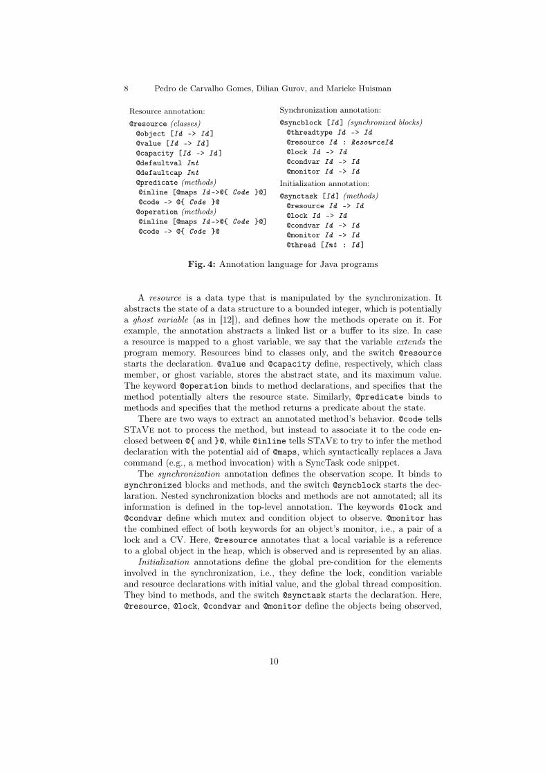
Figure 4 presents the annotation language. Arguments given within squarebrackets are optional, while text within parentheses tells which declaration typesthe annotation binds to. The programmer has to (correctly) provide, by means ofannotations, the following three types of information: resources, synchronizationand initialization.
9
8 Pedro de Carvalho Gomes, Dilian Gurov, and Marieke Huisman
Resource annotation:@resource (classes)@object [Id -> Id ]@value [Id -> Id ]@capacity [Id -> Id ]@defaultval Int@defaultcap Int@predicate (methods)@inline [@maps Id ->@{ Code }@]@code -> @{ Code }@@operation (methods)@inline [@maps Id ->@{ Code }@]@code -> @{ Code }@
Synchronization annotation:@syncblock [Id ] (synchronized blocks)@threadtype Id -> Id@resource Id : ResourceId@lock Id -> Id@condvar Id -> Id@monitor Id -> Id
Initialization annotation:@synctask [Id ] (methods)@resource Id -> Id@lock Id -> Id@condvar Id -> Id@monitor Id -> Id@thread [Int : Id ]
Fig. 4: Annotation language for Java programs
A resource is a data type that is manipulated by the synchronization. Itabstracts the state of a data structure to a bounded integer, which is potentiallya ghost variable (as in [12]), and defines how the methods operate on it. Forexample, the annotation abstracts a linked list or a buffer to its size. In casea resource is mapped to a ghost variable, we say that the variable extends theprogram memory. Resources bind to classes only, and the switch @resourcestarts the declaration. @value and @capacity define, respectively, which classmember, or ghost variable, stores the abstract state, and its maximum value.The keyword @operation binds to method declarations, and specifies that themethod potentially alters the resource state. Similarly, @predicate binds tomethods and specifies that the method returns a predicate about the state.
There are two ways to extract an annotated method’s behavior. @code tellsSTaVe not to process the method, but instead to associate it to the code en-closed between @{ and }@, while @inline tells STaVe to try to infer the methoddeclaration with the potential aid of @maps, which syntactically replaces a Javacommand (e.g., a method invocation) with a SyncTask code snippet.
The synchronization annotation defines the observation scope. It binds tosynchronized blocks and methods, and the switch @syncblock starts the dec-laration. Nested synchronization blocks and methods are not annotated; all itsinformation is defined in the top-level annotation. The keywords @lock and@condvar define which mutex and condition object to observe. @monitor hasthe combined effect of both keywords for an object’s monitor, i.e., a pair of alock and a CV. Here, @resource annotates that a local variable is a referenceto a global object in the heap, which is observed and is represented by an alias.
Initialization annotations define the global pre-condition for the elementsinvolved in the synchronization, i.e., they define the lock, condition variableand resource declarations with initial value, and the global thread composition.They bind to methods, and the switch @synctask starts the declaration. Here,@resource, @lock, @condvar and @monitor define the objects being observed,
10
Specification and Verification of Synchronization with CVs 9
01 class Producer extends Thread {Buffer buffer;
03 Producer(Buffer b){buffer=b;}public void run() {
05 /*@syncblock@monitor buffer -> m
07 @resource buffer:Buffer */synchronized(buffer) {
09 while (buffer.full())buffer.wait();
11 buffer.add();buffer.notifyAll();
13 } } }
15 class Consumer extends Thread {Buffer buffer;
17 Consumer(Buffer b){buffer=b;}public void run() {
19 /*@syncblock@monitor buffer -> m
21 @resource buffer:Buffer */synchronized(buffer) {
23 while (buffer.empty())buffer.wait();
25 buffer.remove();buffer.notifyAll();
27 } } }
29 /*@resource @capacity cap@object els->b_els
31 @value els->b_els */class Buffer {
33 int els; final int cap;/* @operation @inline */
35 void remove(){if (els>0)els--;}/* @operation @inline */
37 void add(){if (els<cap)els++;}/* @predicate @inline */
39 boolean full(){return els==cap;}/* @predicate @inline */
41 boolean empty(){return els==0;}/*@synctask Buffer
43 @monitor b -> m@resource b->b_els */
45 static void main(String[] s) {Buffer b = new Buffer();
47 b.els = 1; b.cap = 1;/* @thread */
49 Consumer c1 = new Consumer(b);/* @thread */
51 Consumer c2 = new Consumer(b);/* @thread */
53 Producer p = new Producer(b);c1.start();p.start();c2.start();
55 } }
Fig. 5: Annotated Java program synchronizing via shared buffer
and assign global aliases to them. Finally, @thread defines that the followingobject corresponds to a spawned thread that synchronizes within the observedsynchronization objects. The object’s type must have been annotated with asynchronization annotation.
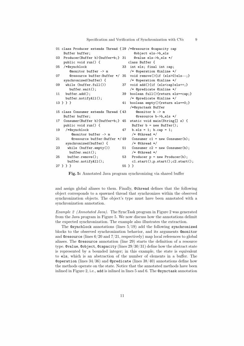
Example 2 (Annotated Java). The SyncTask program in Figure 2 was generatedfrom the Java program in Figure 5. We now discuss how the annotations delimitthe expected synchronization. The example also illustrates the extraction.
The @syncblock annotations (lines 5/19) add the following synchronizedblocks to the observed synchronization behavior, and its arguments @monitorand @resource (lines 6/20 and 7/21, respectively) map local references to globalaliases. The @resource annotation (line 29) starts the definition of a resourcetype. @value, @object, @capacity (lines 29/30/31) define how the abstract stateis represented by a bounded integer; in this example, the state is equivalentto els, which is an abstraction of the number of elements in a buffer. The@operation (lines 34/36) and @predicate (lines 38/40) annotations define howthe methods operate on the state. Notice that the annotated methods have beeninlined in Figure 2, i.e., add is inlined in lines 5 and 6. The @synctask annotation
11
10 Pedro de Carvalho Gomes, Dilian Gurov, and Marieke Huisman
above main starts the declaration of locks, CVs and resources, and @threadannotations add the underneath objects to the global thread composition.
3.2 Synchronization Correctness
The synchronization property of interest here is that “every thread synchroniz-ing under a set of condition variables eventually exits the synchronization”. Wework under the assumption that every such thread eventually reaches its syn-chronization block. There exist techniques (such as [16]) for checking the livenessproperty that a given thread eventually reaches a given control point; checkingvalidity of the above assumption is therefore out of the scope of the present work.
The following definition of correct synchronization applies to a one-time syn-chronization of a Java program. However, if it can be proven that if the initialconditions are the same every time the synchronization scheme is spawned, thenthe scheme is correct for an arbitrary number of invocations. This may be provenby showing that a Java program always resets the variables observed in the syn-chronization before re-spawning the threads.
Definition 1 (Synchronization Correctness). Let P be a Java program witha one-time synchronization such that every thread eventually reaches the entrypoint of its synchronization block. We say that P has a correct synchronizationiff every thread eventually reaches the first control point after the block.
We defined both synchronization correctness and the termination of the cor-responding SyncTask program relative to the correctness of the annotations pro-vided by the programmer. Although out of the scope of the present work, theannotations can potentially be checked, or partially generated, with existingstatic analysis techniques. Further, we assume the memory model of synchro-nized actions in a Java program to be sequentially consistent.
We now connect synchronization schemes of annotated Java programs withSyncTask programs. We shall assume that the programmer has correctly anno-tated the program, as described in Section 3.1.
Theorem 1 (SyncTask Extraction). A correctly annotated Java program hasa correct synchronization iff its corresponding SyncTask terminates.
Proof (Sketch). To prove the result, we define a binary relation R between theconfigurations of the Java program and its SyncTask, and show it to be a weakbisimulation (see [15]), implying that the SyncTask program eventually reaches aterminal configuration (i.e., all threads terminate) if and only if the original Javaprogram has a correct synchronization. We refer to the accompanying technicalreport [5] for the full formalization, and for the most interesting cases, namelythe notify and wait instructions.
The Java annotations define a bidirectional mapping between (some of) theJava program variables and ghost variables and the corresponding bounded vari-ables in SyncTask. Thus, we define R to relate configurations that agree on com-mon variables. Similarly, we define the set of visible transitions as the ones that
12

Specification and Verification of Synchronization with CVs 11
update common variables, and treat all other transitions as silent. We arguethat R is a weak bisimulation in the standard fashion: We establish that (i) theinitial values of the common variables are the same for both programs, and(ii) assuming that observed variables in a Java program are only updated insideannotated synchronized blocks, we establish that any operation that updates acommon variable has the same effect on it in both programs.
To prove (i) it suffices to show that the initial values in the Java program arethe same as the ones provided in the initialization annotation, as described inSection 3. (Here we rely on the correctness of the annotations; however, existingtechniques such as [13,14] can potentially be used for checking this.) The proofof (ii) requires to show that updates to a common variable yield the same resultin both programs. It goes by case analysis on the Java instructions set. Each caseshows that for any configuration pair of R, the operational rules for the givenJava instruction and for the corresponding SyncTask instruction lead to a pairof configurations that again agree on the common variables. As the semanticsof SyncTask presented in Section 2 has been designed to closely mimic the Javasemantics defined in [2], the elaboration of this is straightforward. ⇤
4 Verification of Synchronization Correctness
In this section we show how termination of SyncTask programs can be reducedto a reachability problem on Colored Petri Nets (CPN), and present an experi-mental evaluation of the verification with STaVe and CPN Tools.
4.1 SyncTask Programs as Colored Petri Nets
Various techniques exist to prove termination of concurrent systems. For Sync-Task, it is essential that such a technique efficiently encodes the concurrentthread interleaving, the program’s control flow, synchronization primitives, andbasic data manipulation. Here, we have chosen to reduce the problem of termi-nation of SyncTask programs to a reachability problem on hierarchical CPNsextracted from the program. CPNs allow a natural translation of common lan-guage constructs into CPN components (for this we re-use results from Wester-gaard [18]), and are supported by analysis tools such as CPN Tools. We assumesome familiarity with CPNs, and refer the reader to [7] for a detailed exposition.
The color set THREAD associates a color to each Thread type declara-tion, and a thread is represented by a token with a color from the set. Somecomponents are parametrized by THREAD, meaning that they declare transi-tions, arcs, or places for each thread type. For illustration purposes, we presentthe parametrized components in an example scenario with three thread types:blue (B), red (R), and yellow (Y).
The production rules in Figure 1 are mapped into hierarchical CPN compo-nents, where substitute transitions (STs; depicted as doubly outlined rectangles)represent the non-terminals on the right-hand side. Figure 6a shows the compo-nent for the start symbol SyncTask. The Start place contains all thread tokens in
13
12 Pedro de Carvalho Gomes, Dilian Gurov, and Marieke Huisman
Start
THREAD
End
THREAD
lock
LOCK
1`()
cond
CONDITION
R
Thread_RThread_R
Y
Thread_Y
B
Thread_B
1`R
1`R
1`Y
1`Y
1`B
1`B
Thread_B Thread_Y
cond lock
(a) SyncTask
inportInTHREAD
cond
CONDITION
lock
LOCK
1`()
awaken_B
CONDITION
outportOut
THREAD
waitcond
reacquireLock
1`B (B,B_0)
1`()
(B,B_0)
1`()
1`B
lock
condIn
Outawaken_B
(b) wait
inportIn THREADIn
cond
CONDITION
cond
outportOut THREADOut
awaken_R
CONDITION
awaken_R awaken_Y
CONDITION
awaken_Yawaken_B
CONDITION
awaken_B
flagEmpty_cond wake_R wake_Ywake_B
1`R
1`R
1`R 1`R
1`(R,vcpoint) 1`(R,vcpoint)
1`R
1`R
1`(Y,vcpoint)
1`(Y,vcpoint)
1`R 1`R
1`(B,vcpoint)1`(B,vcpoint)
(c) notify
Fig. 6: Top-level component and condition variables operations
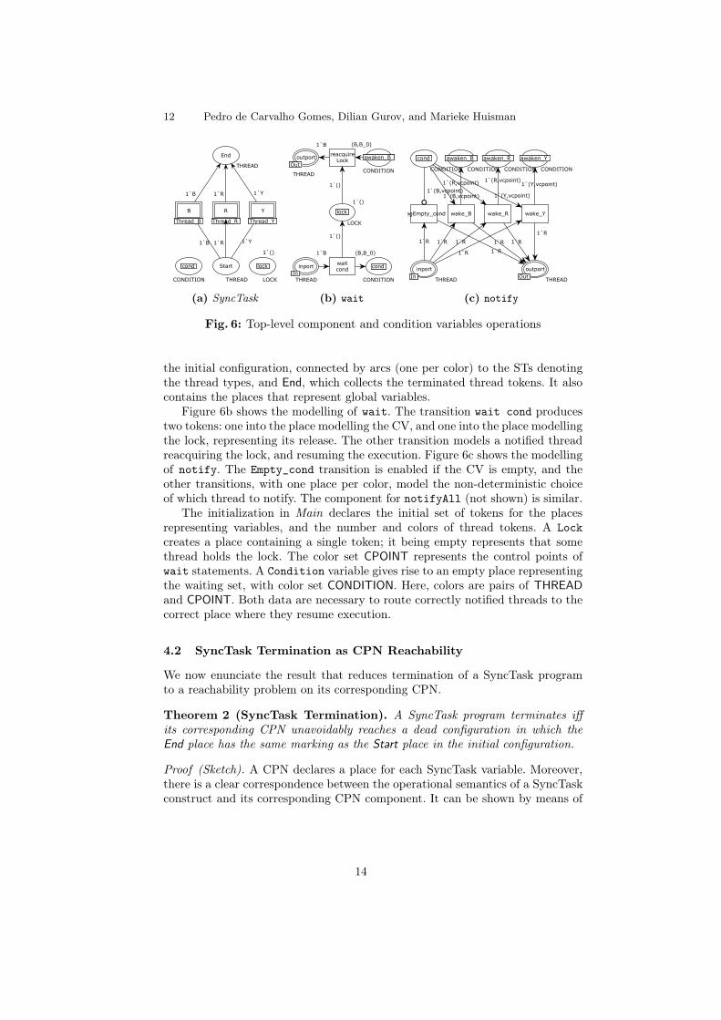
the initial configuration, connected by arcs (one per color) to the STs denotingthe thread types, and End, which collects the terminated thread tokens. It alsocontains the places that represent global variables.
Figure 6b shows the modelling of wait. The transition wait cond producestwo tokens: one into the place modelling the CV, and one into the place modellingthe lock, representing its release. The other transition models a notified threadreacquiring the lock, and resuming the execution. Figure 6c shows the modellingof notify. The Empty_cond transition is enabled if the CV is empty, and theother transitions, with one place per color, model the non-deterministic choiceof which thread to notify. The component for notifyAll (not shown) is similar.
The initialization in Main declares the initial set of tokens for the placesrepresenting variables, and the number and colors of thread tokens. A Lockcreates a place containing a single token; it being empty represents that somethread holds the lock. The color set CPOINT represents the control points ofwait statements. A Condition variable gives rise to an empty place representingthe waiting set, with color set CONDITION. Here, colors are pairs of THREADand CPOINT. Both data are necessary to route correctly notified threads to thecorrect place where they resume execution.
4.2 SyncTask Termination as CPN Reachability
We now enunciate the result that reduces termination of a SyncTask programto a reachability problem on its corresponding CPN.
Theorem 2 (SyncTask Termination). A SyncTask program terminates iffits corresponding CPN unavoidably reaches a dead configuration in which theEnd place has the same marking as the Start place in the initial configuration.
Proof (Sketch). A CPN declares a place for each SyncTask variable. Moreover,there is a clear correspondence between the operational semantics of a SyncTaskconstruct and its corresponding CPN component. It can be shown by means of
14
Specification and Verification of Synchronization with CVs 13
weak bisimulation that every configuration of a SyncTask program is matchedby a unique sequence of consecutive CPN configurations. Therefore, if the Endplace in a dead configuration has the same marking as the Start place in theinitial configuration, then every thread in the SyncTask program terminates itsexecution, for every possible scheduling (note that the non-deterministic threadscheduler is simulated by the non-deterministic firing of transitions). ⇤
CPN termination itself can be verified algorithmically by computing thereachability graph of the generated CPN and checking that: (i) the graph hasno cycles, and (ii) the only reachable dead configurations are the ones where themarking in the End place is the same as the marking in the Start place in theinitial configuration.
4.3 The STaVe Tool
We have implemented the parsing of annotated Java programs to generate Sync-Task programs, and the extraction of hierarchical CPNs from SyncTask, as theSTaVe [4] tool. We now describe the experimental evaluation of our frame-work. This includes the process of annotating Java programs, extraction of thecorresponding CPNs, and the analysis of the nets using CPN Tools.
Our first test case evaluates the scalability of STaVe w.r.t. the size of thepart of program that does not affect the synchronization. For this, we annotatedPIPE [3] (version 4.3.2), a rather large CPN analysis tool written in Java. Itcontains a single (and simple) synchronization scheme using CVs: a thread thatsends logs to a client via a socket waits for a server thread to establish theconnection, and then to notify. This test case illustrates that synchronizationinvolving CVs is typically simple and bounded. Manually annotating the programtook just a few minutes, once the synchronization scheme was understood. TheCPN extraction time was negligible, and the verification process took just a fewmilliseconds to establish the correctness.
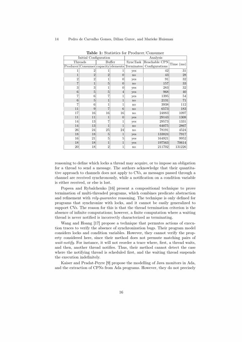
Our second test case evaluates the scalability of STaVe w.r.t. the number ofthreads. We took the example program from Section 2, and instantiated it witha varying number of threads, buffer capacity, and initial value. Table 1 presentsthe practical evaluation for a number of initial configurations.
We observe an expected correlation between the number of tokens represent-ing threads, the size of the state space, and the verification time. Less expectedfor us was the observed influence of the buffer capacities and initial states. Weconjecture that the initial configurations that model high contention, i.e., manythreads waiting on CVs, induce a larger state space. The experiments also showhow termination depends on the thread composition and the initial state. Hence,a single change in any parameter may affect the verification result.
5 Related Work
Leino et al. [14] propose a compositional technique to verify the absence of dead-locks in concurrent systems with both locks and channels. They use deductive
15
14 Pedro de Carvalho Gomes, Dilian Gurov, and Marieke Huisman
Table 1: Statistics for Producer/ConsumerInitial Configuration Analysis
Threads Buffer SyncTask Reachable CPN Time (ms)Producer Consumer capacity elements Terminates Configurations1 2 1 1 yes 42 311 2 2 0 no 43 282 2 1 0 yes 91 327 1 5 0 no 157 333 3 1 0 yes 283 326 5 5 4 yes 968 407 6 7 1 yes 1395 546 5 1 1 no 2131 717 6 1 1 no 3938 112
11 9 7 6 no 6573 18317 16 16 16 no 24883 109711 11 1 0 yes 29143 130814 13 7 1 yes 29573 133114 13 1 1 no 64075 286726 24 25 24 no 78191 452418 18 5 1 yes 133824 791716 21 5 5 yes 164921 995218 18 1 1 yes 197563 7061420 18 2 1 no 211702 131226
reasoning to define which locks a thread may acquire, or to impose an obligationfor a thread to send a message. The authors acknowledge that their quantita-tive approach to channels does not apply to CVs, as messages passed through achannel are received synchronously, while a notification on a condition variableis either received, or else is lost.
Popeea and Rybalchenko [16] present a compositional technique to provetermination of multi-threaded programs, which combines predicate abstractionand refinement with rely-guarantee reasoning. The technique is only defined forprograms that synchronize with locks, and it cannot be easily generalized tosupport CVs. The reason for this is that the thread termination criterion is theabsence of infinite computations; however, a finite computation where a waitingthread is never notified is incorrectly characterized as terminating.
Wang and Hoang [17] propose a technique that permutes actions of execu-tion traces to verify the absence of synchronization bugs. Their program modelconsiders locks and condition variables. However, they cannot verify the prop-erty considered here, since their method does not permute matching pairs ofwait-notify. For instance, it will not reorder a trace where, first, a thread waits,and then, another thread notifies. Thus, their method cannot detect the casewhere the notifying thread is scheduled first, and the waiting thread suspendsthe execution indefinitely.
Kaiser and Pradat-Peyre [9] propose the modelling of Java monitors in Ada,and the extraction of CPNs from Ada programs. However, they do not precisely
16
Specification and Verification of Synchronization with CVs 15
describe how the CPNs are verified, nor provide a correctness argument abouttheir technique. Also, they only validate their tool on toy examples with fewthreads. Our tool is validated on larger test cases, and on a real program.
Kavi et al. [10] present PN components for the synchronization primitives inthe Pthread library for C/C++, including condition variables. However, theirmodelling of CVs just allows the synchronization between two threads, and noargument is presented on how to use it with more threads.
Westergaard [18] presents a technique to extract CPNs for programs in a toyconcurrent language, with locks as the only synchronization primitive. Our workborrows much from this work w.r.t. the CPN modelling and analysis. However,we analyze full-fledged programming languages, and address the complicationsof analyzing programs with condition variables.
Finally, Van der Aalst et al. [1] present strategies for modelling complexparallel applications as CPNs. We borrow many ideas from this work, especiallythe modelling of hierarchical CPNs. However, their formalism is over-complicatedfor our needs, and we therefore simplify it to produce more manageable CPNs.
6 Conclusion
We presented a technique to prove the correct synchronization of Java programsusing condition variables. Correctness here means that if all threads reach theirsynchronization blocks, then all will eventually terminate the synchronization.Our technique does not avoid the exponential blow-up of the state space causedby the interleaving of threads; instead, it alleviates the problem by isolating thesynchronization behavior.
We introduced SyncTask, a simple language to capture the relevant aspects ofsynchronization using condition variables. Also, we define an annotation schemefor programmers to map the expected synchronization in a Java program toa SyncTask program. We establish that the synchronization is correct w.r.t.the above-mentioned property iff the corresponding SyncTask terminates. Asa proof-of-concept, to check termination we define a translation from SyncTaskprograms into Colored Petri Nets such that the program terminates iff thenet invariably reaches a special configuration. The extraction of SyncTask fromannotated Java programs, and the translation to CPNs, is implemented as theSTaVe tool. We validate our technique on some test-cases using CPN Tools.
Our current results hold for a number of restrictions on the analyzed pro-grams. In future work we plan to address and relax these restrictions, integratespecial-purpose static analyzers for the separate types of required annotations,incorporate more sophisticated model checkers for checking termination of Sync-Task programs, and perform a more diverse experimental evaluation and com-parison with other verification techniques.
17
16 Pedro de Carvalho Gomes, Dilian Gurov, and Marieke Huisman
References
1. van der Aalst, W., Stahl, C., Westergaard, M.: Strategies for modeling complexprocesses using colored Petri nets. In: Transactions on Petri Nets and Other Modelsof Concurrency VII, LNCS, vol. 7480, pp. 6–55. Springer Berlin Heidelberg (2013)
2. Cenciarelli, P., Knapp, A., Reus, B., Wirsing, M.: An event-based structural op-erational semantics of multi-threaded Java. In: Formal Syntax and Semantics ofJava, LNCS, vol. 1523, pp. 157–200. Springer Berlin Heidelberg (1999)
3. Dingle, N.J., Knottenbelt, W.J., Suto, T.: PIPE2: A tool for the performanceevaluation of generalised stochastic Petri nets. SIGMETRICS 36(4), 34–39 (2009)
4. Gomes, P.: SyncTAsk VErifier. http://www.csc.kth.se/~pedrodcg/stave (2015)5. Gomes, P.d.C., Gurov, D., Huisman, M.: Algorithmic verification of multithreaded
programs with condition variables. Tech. rep., KTH Royal Institute of Technology(October 2015), http://urn.kb.se/resolve?urn=urn:nbn:se:kth:diva-176006
6. Hoare, C.A.R.: Monitors: An operating system structuring concept. Commun.ACM 17(10), 549–557 (Oct 1974)
7. Jensen, K., Kristensen, L.M.: Coloured Petri Nets: Modelling and Validation ofConcurrent Systems. Springer Publishing Company, Incorporated, 1st edn. (2009)
8. Jensen, K., Kristensen, L., Wells, L.: Coloured Petri nets and CPN tools for mod-elling and validation of concurrent systems. International Journal on Software Toolsfor Technology Transfer 9(3-4), 213–254 (2007)
9. Kaiser, C., Pradat-Peyre, J.F.: Weak fairness semantic drawbacks in Java multi-threading. In: Proceedings of the 14th Ada-Europe International Conference onReliable Software Technologies. pp. 90–104. Springer-Verlag (2009)
10. Kavi, K., Moshtaghi, A., Chen, D.j.: Modeling multithreaded applications usingPetri nets. International Journal of Parallel Programming 30(5), 353–371 (2002)
11. Lamport, L.: How to make a multiprocessor computer that correctly executes mul-tiprocess programs. IEEE Trans. Comput. 28(9), 690–691 (Sep 1979)
12. Leavens, G., Baker, A., Ruby, C.: JML: A notation for detailed design. In: Kilov,H., Rumpe, B., Simmonds, I. (eds.) Behavioral Specifications of Businesses andSystems, Eng. and Comp. Sci., vol. 523, pp. 175–188. Springer US (1999)
13. Leino, K.R., Müller, P.: A basis for verifying multi-threaded programs. In: Proceed-ings of the 18th European Symposium on Programming Languages and Systems.pp. 378–393. ESOP ’09, Springer-Verlag, Berlin, Heidelberg (2009)
14. Leino, K.R.M., Müller, P., Smans, J.: Deadlock-free channels and locks. In: Euro-pean Conference on Programming Languages and Systems. pp. 407–426. ESOP’10,Springer-Verlag (2010)
15. Milner, R.: Communicating and mobile systems: the ⇡-calculus, chap. 6, pp. 52–53.Cambridge University Press, New York, NY, USA (1999)
16. Popeea, C., Rybalchenko, A.: Compositional termination proofs for multi-threadedprograms. In: Tools and Algorithms for the Construction and Analysis of Systems.pp. 237–251. TACAS’12, Springer-Verlag (2012)
17. Wang, C., Hoang, K.: Precisely deciding control state reachability in concurrenttraces with limited observability. In: Verification, Model Checking, and AbstractInterpretation, LNCS, vol. 8318, pp. 376–394. Springer Berlin Heidelberg (2014)
18. Westergaard, M.: Verifying parallel algorithms and programs using coloured Petrinets. In: Transactions on Petri Nets and Other Models of Concurrency VI, LNCS,vol. 7400, pp. 146–168. Springer Berlin Heidelberg (2012)
18
An interval logic for stream-processing functions:A convolution-based construction
Brijesh Dongol
Department of Computer Science, Brunel University, UK
Abstract. We develop an interval-based logic for reasoning about sys-tems consisting of component specified using stream-processing func-tions, which map streams of inputs to streams of outputs. The construc-tion is algebraic and builds on a theory of convolution from formal powerseries. Using these algebraic foundations, we uniformly (and systemat-ically) define operators for time- and space-based (de)composition. Wealso show that Banach’s fixed point theory can be incorporated into theframework, building on an existing theory of partially ordered monoids,which enables a feedback operator to be defined algebraically.
1 Introduction
Many systems (e.g., hybrid systems) require logics that are capable of reasoningabout both discrete and continuous behaviours; scalability in reasoning methodsfor such systems has long been an open challenge. Especially di�cult is a logicthat enables reasoning about time- and space-based properties, including feed-back, to be (de-)composed in a uniform manner. From a uniformity perspective,one way forward is the development of logics and reasoning frameworks fromalgebraic foundations [12].
In this paper, we build on our previous work on convolution [8], which isa concept taken from formal power series [9, 2]. Essentially, convolution definesmultiplication for functions of type QM = M ! Q , where M is a partial monoid(see Section 3) and Q is a quantale (see Section 5). For any x 2 M , the convo-lution of f , g 2 QM is given by
(f · g) x =X
x=y�zf y � g z .
That is, multiplication · at the level of the functions f and g is defined as thesum of all possible decompositions of the argument x into components y and z ,where x = y � z and each term in the sum is obtained by applying f to y and gto z , then multiplying the results of the function applications using �.
There are many possible instantiations of M and Q , which allows the algebrato capture many di↵erent models of computation (see [8] for details). As we shallsee, in this paper, the quantale Q that we consider is a boolean quantale, and Mitself has a richer algebraic structure. In particular, we use a monoidal structureM consisting of three di↵erent multiplication operators: one for (de)composing
19
yn
. . . fx2
x1
xm
. . .
y1y2
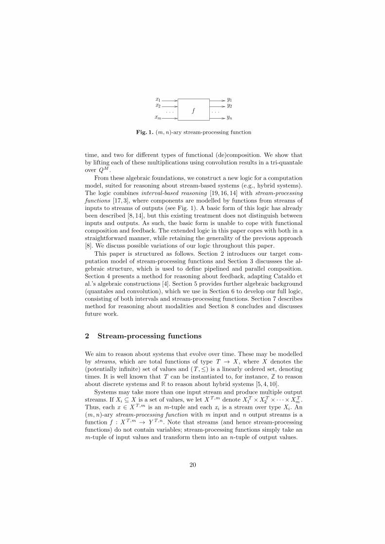
Fig. 1. (m,n)-ary stream-processing function
time, and two for di↵erent types of functional (de)composition. We show thatby lifting each of these multiplications using convolution results in a tri-quantaleover QM .
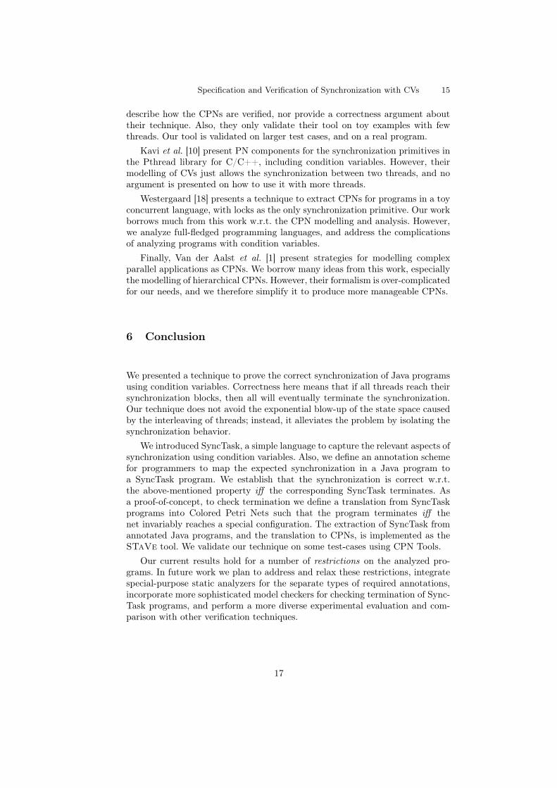
From these algebraic foundations, we construct a new logic for a computationmodel, suited for reasoning about stream-based systems (e.g., hybrid systems).The logic combines interval-based reasoning [19, 16, 14] with stream-processingfunctions [17, 3], where components are modelled by functions from streams ofinputs to streams of outputs (see Fig. 1). A basic form of this logic has alreadybeen described [8, 14], but this existing treatment does not distinguish betweeninputs and outputs. As such, the basic form is unable to cope with functionalcomposition and feedback. The extended logic in this paper copes with both in astraightforward manner, while retaining the generality of the previous approach[8]. We discuss possible variations of our logic throughout this paper.
This paper is structured as follows. Section 2 introduces our target com-putation model of stream-processing functions and Section 3 discussses the al-gebraic structure, which is used to define pipelined and parallel composition.Section 4 presents a method for reasoning about feedback, adapting Cataldo etal.’s algebraic constructions [4]. Section 5 provides further algebraic background(quantales and convolution), which we use in Section 6 to develop our full logic,consisting of both intervals and stream-processing functions. Section 7 describesmethod for reasoning about modalities and Section 8 concludes and discussesfuture work.
2 Stream-processing functions
We aim to reason about systems that evolve over time. These may be modelledby streams, which are total functions of type T ! X , where X denotes the(potentially infinite) set of values and (T ,) is a linearly ordered set, denotingtimes. It is well known that T can be instantiated to, for instance, Z to reasonabout discrete systems and R to reason about hybrid systems [5, 4, 10].
Systems may take more than one input stream and produce multiple outputstreams. If Xi ✓ X is a set of values, we let XT ,m denote XT
1 ⇥XT2 ⇥ · · ·⇥XT
m .Thus, each x 2 XT ,m is an m-tuple and each xi is a stream over type Xi . An(m,n)-ary stream-processing function with m input and n output streams is afunction f : XT ,m ! Y T ,n . Note that streams (and hence stream-processingfunctions) do not contain variables; stream-processing functions simply take anm-tuple of input values and transform them into an n-tuple of output values.
20
Although a stream-processing function (of type XT ) defines values over alltime in T , reasoning typically only takes place after initialisation. For conve-nience, we assume 0 2 T and that stream-processing functions are initialised attime 0.
One of the benefits of using stream-processing functions (which naturallydistinguish between input/output streams) is that they simplify reasoning aboutfeedback. In order to ensure feedback is well defined, we require that the streamsare -causal, with some delay . A stream-processing function is causal i↵ itsinput until time t � 0 completely determines its output until time t , and is -causal i↵ its input until time t � 0 completely determines its output until timet + (where > 0). (Delayed) causality imposes the basic requirement thata system cannot anticipate the future values of its inputs. These concepts areformalised below. We use notation f =t g to denote 8u 2 T . u t ) f u = g u,where, following algebraic conventions, we write f x for function application f (x ).
Definition 1. Let f be an (m,n)-ary stream-processing function. We say f iscausal i↵
8x , x 0 2 XT ,m , t 2 T�0 . (x =t x 0) ) (f x =t f x 0)
and that f is -causal with delay > 0 i↵
8x , x 0 2 XT ,m , t 2 T�0 . (x =t x 0) ) (f x =t+ f x 0).
We will refer to a causal stream-processing function as a behaviour and a -causalstream-processing function as a delayed behaviour.
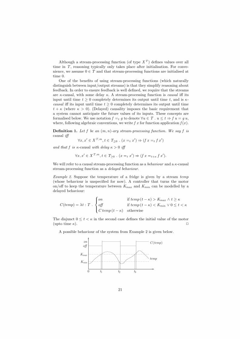
Example 2. Suppose the temperature of a fridge is given by a stream temp(whose behaviour is unspecified for now). A controller that turns the motoron/o↵ to keep the temperature between Kmax and Kmin can be modelled by adelayed behaviour:
C (temp) = �t : T .
8><>:
on if temp (t � ) > Kmax ^ t �
o↵ if temp (t � ) < Kmin _ 0 t <
C temp (t � ) otherwise
The disjunct 0 t < in the second case defines the initial value of the motor(upto time ). 2
A possible behaviour of the system from Example 2 is given below.
o↵
on
Kmin
0
Kmax
t1 t2 t3
C (temp)
temp
21
The temperature temp fluctuates between Kmax an Kmin . The stream processingfunction C takes temp as input and transforms it into some output C (temp)resulting in the values on or o↵ . Note the delay between the value of temprising above Kmax (e.g., at t1) and the output on, as well as the value of tempdipping below Kmin (e.g., at t2) and the output o↵ .
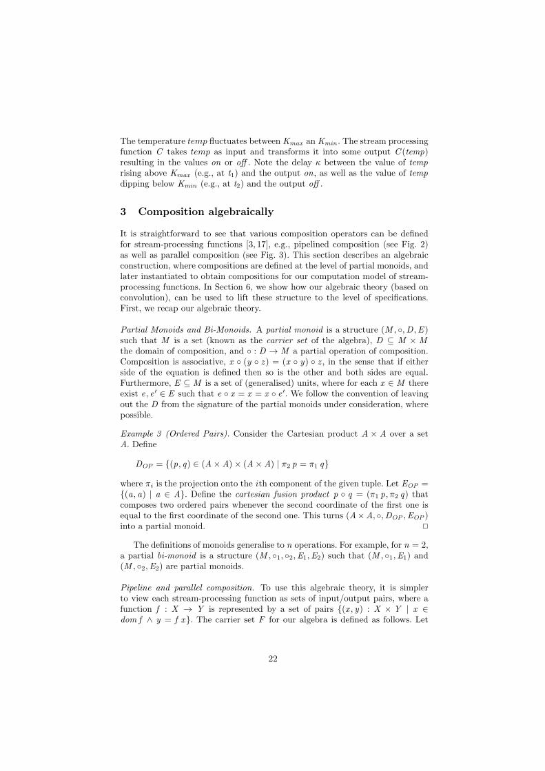
3 Composition algebraically
It is straightforward to see that various composition operators can be definedfor stream-processing functions [3, 17], e.g., pipelined composition (see Fig. 2)as well as parallel composition (see Fig. 3). This section describes an algebraicconstruction, where compositions are defined at the level of partial monoids, andlater instantiated to obtain compositions for our computation model of stream-processing functions. In Section 6, we show how our algebraic theory (based onconvolution), can be used to lift these structure to the level of specifications.First, we recap our algebraic theory.
Partial Monoids and Bi-Monoids. A partial monoid is a structure (M , �,D ,E )such that M is a set (known as the carrier set of the algebra), D ✓ M ⇥ Mthe domain of composition, and � : D ! M a partial operation of composition.Composition is associative, x � (y � z ) = (x � y) � z , in the sense that if eitherside of the equation is defined then so is the other and both sides are equal.Furthermore, E ✓ M is a set of (generalised) units, where for each x 2 M thereexist e, e 0 2 E such that e � x = x = x � e 0. We follow the convention of leavingout the D from the signature of the partial monoids under consideration, wherepossible.
Example 3 (Ordered Pairs). Consider the Cartesian product A ⇥ A over a setA. Define
DOP = {(p, q) 2 (A ⇥ A) ⇥ (A ⇥ A) | ⇡2 p = ⇡1 q}
where ⇡i is the projection onto the ith component of the given tuple. Let EOP ={(a, a) | a 2 A}. Define the cartesian fusion product p � q = (⇡1 p,⇡2 q) thatcomposes two ordered pairs whenever the second coordinate of the first one isequal to the first coordinate of the second one. This turns (A⇥A, �,DOP ,EOP )into a partial monoid. 2
The definitions of monoids generalise to n operations. For example, for n = 2,a partial bi-monoid is a structure (M , �1, �2,E1,E2) such that (M , �1,E1) and(M , �2,E2) are partial monoids.
Pipeline and parallel composition. To use this algebraic theory, it is simplerto view each stream-processing function as sets of input/output pairs, where afunction f : X ! Y is represented by a set of pairs {(x , y) : X ⇥ Y | x 2dom f ^ y = f x}. The carrier set F for our algebra is defined as follows. Let
22
yn
. . . fx2
x1
xm
g . . .. . .
y1y2
Fig. 2. Pipelined composition f >> g
Fm,n = XT ,m ⇥ Y T ,n be the set of all (m,n)-ary input/output tuples and letF =
Sm,n:N Fm,n be the set of all input/output tuples. Also let id be the identity
function.Pipeline composition takes all output messages from the first component and
uses them as inputs to the second (see Fig. 2).
Lemma 4 (Pipeline composition). (F , >>, id) is a partial monoid with de-finedness relation DOP .
a1
. . . fx2
x1
xm
. . .
g . . .. . .
y1y2
yn
bl
b2
b1
ak
a2
Fig. 3. Parallel composition f ⌦ g
y
f
g
c1 c2
x1 y1
x2 y2
x
Fig. 4. Duplicating/combining inputs/outputs
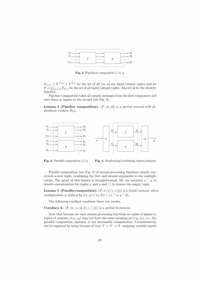
Parallel composition (see Fig. 3) of stream-processing functions simply con-structs a new tuple, combining the first and second arguments to the multipli-
cation. The proof of this lemma is straightforward. We use notation x a y todenote concatenation for tuples x and y and h i to denote the empty tuple.
Lemma 5 (Parallel composition). (F ,⌦, {(h i, h i)}) is a (total) monoid, where
multiplication is defined by ((x , y) ⌦ (a, b)) = (x a a, y a b).
The following corollary combines these two results.
Corollary 6. (F , >>,⌦, id, {(h i, h i)}) is a partial bi-monoid.
Note that because we view stream-processing functions as tuples of inputs totuples of outputs, f (x1, x2) may not have the same meaning as f (x2, x1), i.e., theparallel composition operator is not necessarily commutative. Commutativitycan be regained by using streams of type T ! V ! X , mapping variable names
23
V to values X . We leave the study of the (more complicated) stream processingfunctions that result from these as a topic of future study.
Clearly, it should be possible for two components operating in parallel toshare inputs, or produce an output that combines the outputs of the two com-ponents. Such situations can be easily modelled by defining for instance, a dupli-cator that splits some shared input stream into two disjoint outputs. Similarly,outputs can be combined by a stream-processing function that collates, com-bines and processes outputs from several parallel sources. An example is givenin Fig. 4, which defines the component c1 >> (f ⌦ g) >> c2.
4 Feedback
The streams under consideration are over a linear order T . For such models,the use of Banach’s theory to ensure the existence of a unique fixed point iswell known [17, 4]. This includes constructive fixed-point theorems that enablecalculation of this unique fixed point [4]. We recap Cataldo et al.’s main result(and the background needed to understand this result); then apply it to oursetting of (m,n)-ary stream-processing functions.
Feedback algebraically. Following Cataldo et. al., the generalisation of Banach’sfixed-point theory is given in terms of a pomonoid (as in partially orderedmonoid), which is a structure (�,v,�,?) such that (�,�,?) is a monoid and(�,v) is a partial order with minimum element ?. Given a set X and a pomonoid(�,v,�,?), we define a petric (as in pomonoid metric) to be any d : X ⇥X ! �such that for all x , y , z 2 X :
1. d x y = ? i↵ x = y ,2. d x y = d y x , and3. d x z v d x y � d y z
For example, any metric is a petric over the pomonoid (R�0,, +, 0).An infinite sequence G = (�0, �1, . . . ) 2 �! is decaying i↵ for all � 2 �\{?}
there exists an n 2 N such that for all k � n, �k @ �, i.e., for any non-zero value�, there is a point in G where the elements from that point onwards are below�. An infinite sequence Xs = (x0, x1, . . . ) 2 X ! is Cauchy i↵ for all � 2 �\{?},there exists an n 2 N such that for all k ,m � n, (d xk xm) @ �. We say thatXs converges to x 2 X i↵ the sequence ((d x0 x ), (d x1 x ), . . . ) 2 �! is decaying.The set X is Cauchy complete i↵ for all Cauchy sequences (x0, x1, . . . ) 2 X !,there exists a unique x 2 X such that the sequence (x0, x1, . . . ) converges to x .
These definitions are used to define a scheme for constructing the fixed pointof a function f : X ! X , given by the following recursion, where i � 0:
f 0 x = x f i+1 x = f (f i x )
We say f is a strict contraction i↵ 8x , y 2 X . x 6= y ) d (f x ) (f y) @ d x yfor some petric d . For a discrete time domain, a strict contraction is enough to
24
. . .
. . .x2
x1
xm
. . .
y1y2
yn
f
. . .
z1z2
zk
Fig. 5. Feedback composition µk f
ensure a fixed-point is reached. Given x , y 2 X and n 2 N, let
Bn x y =nLk
i=n d (f i x ) (f i y) | k 2 N ^ k � no
A strict contraction f is a decaying contraction i↵ for all x , y 2 X , there existsa decaying sequence (�0, �1, ...) 2 �! where �n is an upper bound for Bn x y .
Theorem 7 ([4]). If X is Cauchy complete with respect to petric d, and iff : X ! X is a decaying contraction, then f has a unique fixed point fix (f ) 2 X .Moreover, for any x 2 X , the sequence ((f 0 x ), (f 1 x ), ...) converges to fix (f ).
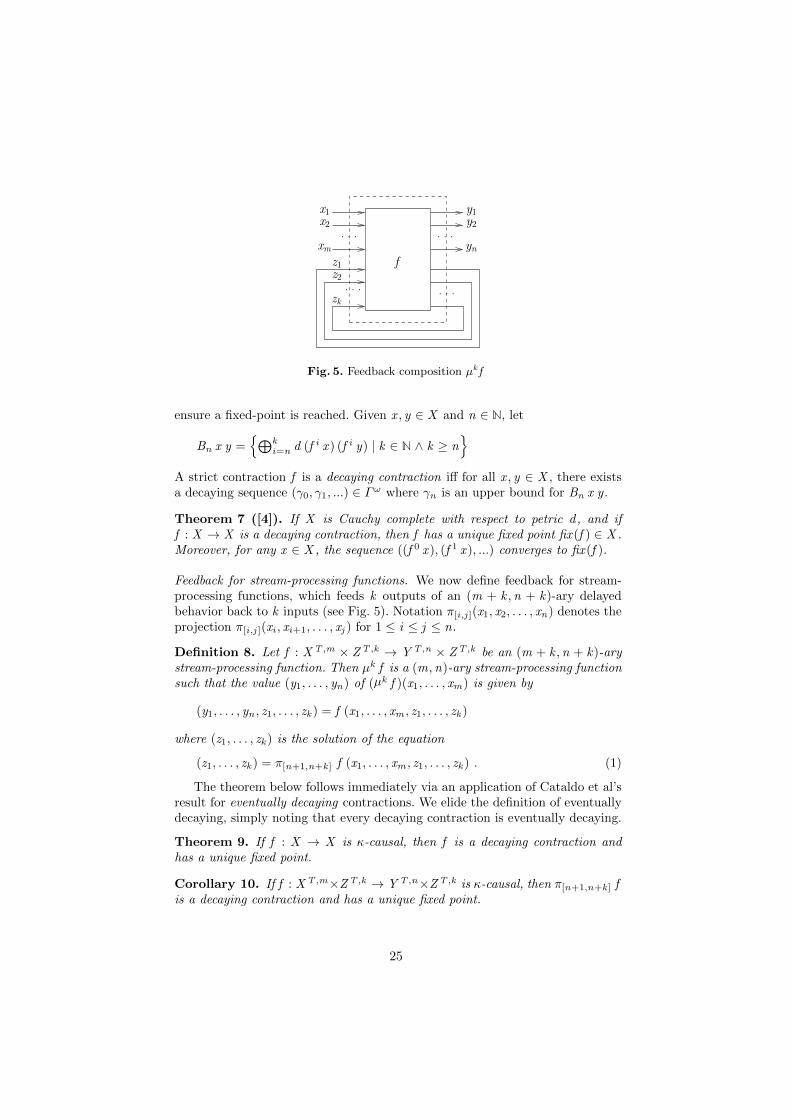
Feedback for stream-processing functions. We now define feedback for stream-processing functions, which feeds k outputs of an (m + k ,n + k)-ary delayedbehavior back to k inputs (see Fig. 5). Notation ⇡[i,j ](x1, x2, . . . , xn) denotes theprojection ⇡[i,j ](xi , xi+1, . . . , xj ) for 1 i j n.
Definition 8. Let f : XT ,m ⇥ ZT ,k ! Y T ,n ⇥ ZT ,k be an (m + k ,n + k)-arystream-processing function. Then µk f is a (m,n)-ary stream-processing functionsuch that the value (y1, . . . , yn) of (µk f )(x1, . . . , xm) is given by
(y1, . . . , yn , z1, . . . , zk ) = f (x1, . . . , xm , z1, . . . , zk )
where (z1, . . . , zk ) is the solution of the equation
(z1, . . . , zk ) = ⇡[n+1,n+k ] f (x1, . . . , xm , z1, . . . , zk ) . (1)
The theorem below follows immediately via an application of Cataldo et al’sresult for eventually decaying contractions. We elide the definition of eventuallydecaying, simply noting that every decaying contraction is eventually decaying.
Theorem 9. If f : X ! X is -causal, then f is a decaying contraction andhas a unique fixed point.
Corollary 10. If f : XT ,m⇥ZT ,k ! Y T ,n⇥ZT ,k is -causal, then ⇡[n+1,n+k ] fis a decaying contraction and has a unique fixed point.
25
Example 11. Consider the controller in Example 2 operating in parallel with anenvironment (which modifies temp) depending on the value of the motor. Wedefine
CE (motor) = �t : T . if motor t = on then lower t else raise t
where we assume lower (respectively, raise) is a continuous monotonically de-creasing (increasing) function describing the rate of change of temp. The overallsystem is described by the composition: µ1(C >> CE ). This function is well-defined since its fixed point is uniquely determined. C >> CE is contractive withdelay , and hence, Corollary 10 can be applied.
5 Quantales and power series
The framework we have defined thus far enables reasoning about and composingstream-processing functions. We wish to extend this into a reasoning framework,and to this end, incorporate an interval temporal logic [10, 5, 16, 19], which maybe used to reason about the safety, liveness, and real-time properties that asystem possesses. It turns out that this extension can be constructed using analgebraic approach, by lifting the notion of a stream-processing function to abehaviour, which is a predicate over a stream-processing function and an interval.
This section presents the algebraic underpinnings to make the above aimspossible. A quantale is a structure (Q ,, ·, 1) such that (Q ,) is a completelattice, (Q , ·, 1) is a monoid and the distributivity axioms
(X
i2I
xi) · y =X
i2I
(xi · y), x · (X
i2I
yi) =X
i2I
(x · yi)
hold, whereP
X denotes the supremum of a set X ✓ Q . We write 0 and U forthe least and the greatest elements of the quantale with respect to . The twoannihilation laws x · 0 = 0 = 0 · x hold in any quantale.
Example 12. The quantale of booleans B = {0, 1} with 0 1, binary supremumor join t and composition as binary infimum or meet x · y = x u y plays animportant role for interval logics. It also satisfies distributivity laws with respectto join and meet and every element is complemented.
Convolution. The algebraic foundations for this paper is based on power seriesfrom formal languages, which provides mechanisms for lifting properties of theunderlying algebraic structures to the level of functions over these structures.More formally, a power series is a function f : M ! Q from a partial monoid Minto a quantale Q . Operators on f are defined by lifting operators on M and Qas follows. For f , g : M ! Q , an index set I , a family of functions fi : M ! Qand i 2 I , we define
(X
i2I
fi) x =X
i2I
fi x (f · g) x =X
x=y�z(f y) � (g z )
26
Note that the first operation is just pointwise lifting with (f +g) x = f x +g x asa special case. The composition f · g is called convolution. The variables y andz underneath the sum are implicitly existentially quantified. A more precise butless convenient notation is (f ·g) x =
P{q 2 Q | 9y , z . x = y �z ^q = f y�g z}.The sum is lifted pointwise; (f + g) x = f x + g x arises as a special case. Inaddition, we define the O : M ! Q and 1 : M ! Q by
O x = 0, 1 x = if x 2 E then 1 else 0.
Hence O is the constant function that returns value 0 and 1 is the subobjectclassifier for E . The quantale structure lifts from Q to the function space QM
of power series.
Theorem 13 ([8]). Let (M , �,D ,E ) be a partial monoid. If (Q ,,�, 1) is aunital quantale, then so is (QS ,, ·, 1).
The order on QM is obtained from that on Q by pointwise lifting: f g i↵f x g x holds for all x 2 M .
There are a variety of instantiations for quantale QM . Here, we are mainlyinterested in the quantale BM ⇠= P M of power series of type M ! B into thequantale of booleans, which is the power set quantale of the partial monoid M .In this instance, convolution becomes
(p · q) x =X
x=y�zp y u q z .
Moreover, 1 = E is a boolean-valued function, hence 1 x holds i↵ x 2 E . Theboolean algebra structure of B is preserved by the lifting to BM . Hence distribu-tive laws between join and meet hold and boolean complements of predicatescan be defined.
As with monoids, it is possible to extend quantales with more than onemultiplication operator. For example, a bi-quantale is a structure (Q ,, ·1, ·2)such that (Q ,, ·1) and (Q ,, ·2) are quantales. A bi-quantale is unital i↵ bothits multiplications have units.
6 Interval-stream specifications
With the necessary algebraic background in place, we develop our interval-basedreasoning framework. The basis for this work is a specification construct thatdefines behaviours of system components using interval-stream predicates, whichare predicates over an interval and an (m,n)-ary stream-processing function.
Formally, we assume I (T ) = {[a, b] | a, b 2 T ^ a b} denotes the set of all(closed) intervals over the linear poset (T ,). An interval-stream predicate hastype I (T )⇥F ! B, mapping a given interval and stream-processing function toa boolean. Interval stream predicates can be understood as expressing propertiesof a stream-processing function f applied to an interval '. They are similar tohigher-order functions such as maps or folds in functional programming.
27
Example 14. Consider the specification of a system that controls a motor de-pending on the input value of the temp. Suppose we wish to specify that themotor is on at the end of any interval ' in which temp stays above Kmax . Thismay be formalised by the interval-stream predicate React , where:
React ' (temp, motor) = (8t : ' . temp t > Kmax ) ) motor (max ') = on
Now recall the controller C from Example 2. Clearly, React ' (temp,C temp)does not necessarily hold because � may refer to a time prior to system initiali-sation, or C may not have enough time to react within �. However, it is possibleto show that, for any ' such that min ' � 0 and max ' � min ' > , we haveReact ' (temp,C temp). 2
Combining intervals and stream-processing functions algebraically. We developan algebraic construction of interval-stream predicates using our convolution-based liftings. First, we must understand the algebraic structure of intervals. Itis straightforward to show that intervals form a partial monoid. Let
DCI = {(a, b) 2 I (T ) ⇥ I (T ) | max a = min b} ECI = {[t , t ] | t 2 T}
be the domain of composition and set of all point intervals, respectively. De-fine the interval fusion product a ; b = a [ b that composes two intervals[t1, t2] and [u1, u2] by taking their union [t1, t2] whenever t2 = u1. This turns(I (T ), ;,D ,ECI ) into a partial monoid.
Note 15. An algebraic treatment of semi-open intervals can also be given [8],which leads to an alternative interval logic [5] that simplifies reasoning aboutdiscontinuities when discrete values change. However, because such a logic ismore complex, we leave out this variation in this paper, and consider full devel-opment of such a framework to be future work.
Recall that we have already established that partial stream-processing func-tions form a bi-monoid (Corollary 6). Combining this result with the intervalmonoid results in a carrier set of type M = I (T ) ⇥ F and three partial multi-plication operators:
– ; that operates as chop on the intervals;– >> that operates as pipeline on the stream-processing functions; and– ⌦ that operates as parallel composition on the stream-processing functions.
This results in a partial tri-monoid (M, ;, >>,⌦, bECI , bE>>, bE⌦), where:
(z1, f ) ; (z2, f ) = (z1 ; z2, f )
(z , f1) >> (z , f2) = (z , f1 >> f2)
(z , f1) ⌦ (z , f2) = (z , f1 ⌦ f2)
define the three monoidal operations. The chop operates on the interval compo-nent, leaving the stream-processing function unchanged, while the pipeline and
28
parallel composition operators are applied to the functional component, leavingthe interval component unchanged.
The definedness relation for the partial relations are given by lifting thedefinedness relations to the level of the cross product:
D; = {(x1, f1) ⇥ (x2, f2) | (x1, x2) 2 DCI ^ f2 = f2}D>> = {(x1, f1) ⇥ (x2, f2) | x1 = x2 ^ (f1, f2) 2 DOP}D⌦ = {(x1, f1) ⇥ (x2, f2) | x1 = x2 ^ (f1, f2) 2 DPC}
The unit sets are bECI = {(i , f ) | i 2 ECI ^ f 2 F}, bE>> = {(i , f ) | i 2 I (T ) ^f 2 id} and bE⌦ = {(i ,?) | i 2 I (T )}.
Tri-quantales. Our aim is to lift these monoidal operations to the level of theinterval-stream predicates using convolution. First we define the generic theoryover the structure QM1⇥M2 , where M1 is a monoid, M2 is a bimonoid and Q isquantale.
Theorem 16 below shows that this lifting gives us a tri-quantale structure inthe generic case when the target algebra is a quantale. Later, we will instantiatethis theorem and obtain our theory of interval predicates. Suppose (M1, �1,E1) isa partial monoid, and (M2, �2, �3,E2,E3) a partial bi-monoid. Define a structure
Q = (QM1⇥M2 ,, ·1, ·2, ·3, 11, 12, 13)
where the three multiplication operators over QM1⇥M2 are defined using convo-lution as follows for p, q 2 QM1⇥M2 :
(p ·1 q) (', f ) =X
'='1�1'2
p ('1, f ) � q ('2, f )
(p ·2 q) (', f ) =X
f =f1�2f2
p (', f1) � q (', f2)
(p ·3 q) (', f ) =X
f =f1�3f2
p (', f1) � q (', f2)
Theorem 16. If (M1, �1,E1) is a partial monoid, (M2, �2, �3,E2,E3) is a partialbi-monoid and (Q ,, �) is a unital quantale, then Q is a tri-quantale. Further-more, if (Q ,, �) is distributive, then so is Q.
As an example, we verify the unit law for the first multiplication operator.
(11 ·1 q) (', f )
=X
'='1�1'2
11 ('1, f ) � q ('2, f )
= (X
('=e�1')e2E1
11 (e, f ) � q (', f )) + (X
'='1�1'2'1 62E1
11 ('1, f ) � q ('2, f ))
29
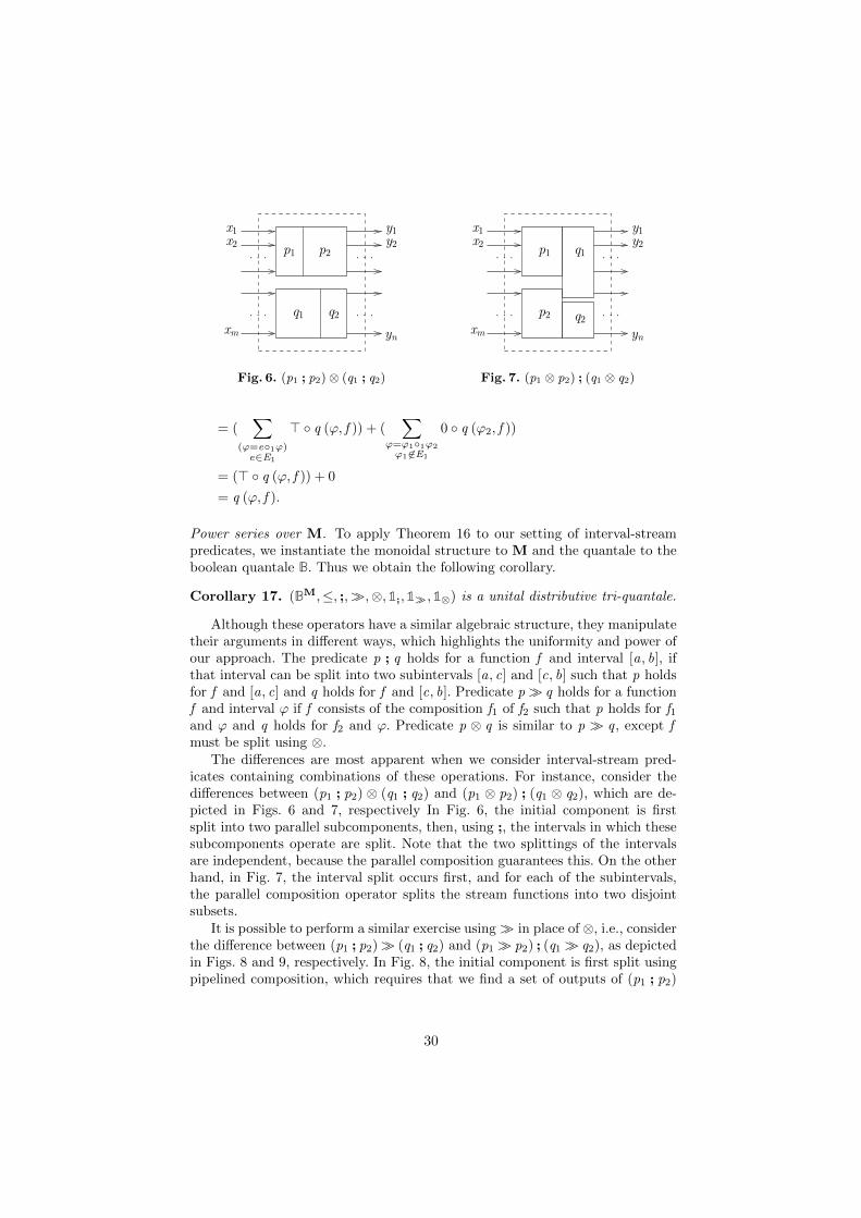
. . .
x2
x1 y1y2
ynxm
p1
q1
p2
q2. . .
. . . . . .
Fig. 6. (p1 ; p2) ⌦ (q1 ; q2)
q2
x2
x1 y1y2
ynxm
. . .
. . . . . .
. . .
p1 q1
p2
Fig. 7. (p1 ⌦ p2) ; (q1 ⌦ q2)
= (X
('=e�1')e2E1
> � q (', f )) + (X
'='1�1'2'1 62E1
0 � q ('2, f ))
= (> � q (', f )) + 0
= q (', f ).
Power series over M. To apply Theorem 16 to our setting of interval-streampredicates, we instantiate the monoidal structure to M and the quantale to theboolean quantale B. Thus we obtain the following corollary.
Corollary 17. (BM,, ;, >>,⌦, 1;, 1>>, 1⌦) is a unital distributive tri-quantale.
Although these operators have a similar algebraic structure, they manipulatetheir arguments in di↵erent ways, which highlights the uniformity and power ofour approach. The predicate p ; q holds for a function f and interval [a, b], ifthat interval can be split into two subintervals [a, c] and [c, b] such that p holdsfor f and [a, c] and q holds for f and [c, b]. Predicate p >> q holds for a functionf and interval ' if f consists of the composition f1 of f2 such that p holds for f1and ' and q holds for f2 and '. Predicate p ⌦ q is similar to p >> q , except fmust be split using ⌦.
The di↵erences are most apparent when we consider interval-stream pred-icates containing combinations of these operations. For instance, consider thedi↵erences between (p1 ; p2) ⌦ (q1 ; q2) and (p1 ⌦ p2) ; (q1 ⌦ q2), which are de-picted in Figs. 6 and 7, respectively In Fig. 6, the initial component is firstsplit into two parallel subcomponents, then, using ;, the intervals in which thesesubcomponents operate are split. Note that the two splittings of the intervalsare independent, because the parallel composition guarantees this. On the otherhand, in Fig. 7, the interval split occurs first, and for each of the subintervals,the parallel composition operator splits the stream functions into two disjointsubsets.
It is possible to perform a similar exercise using >> in place of ⌦, i.e., considerthe di↵erence between (p1 ; p2) >> (q1 ; q2) and (p1 >> p2) ; (q1 >> q2), as depictedin Figs. 8 and 9, respectively. In Fig. 8, the initial component is first split usingpipelined composition, which requires that we find a set of outputs of (p1 ; p2)
30
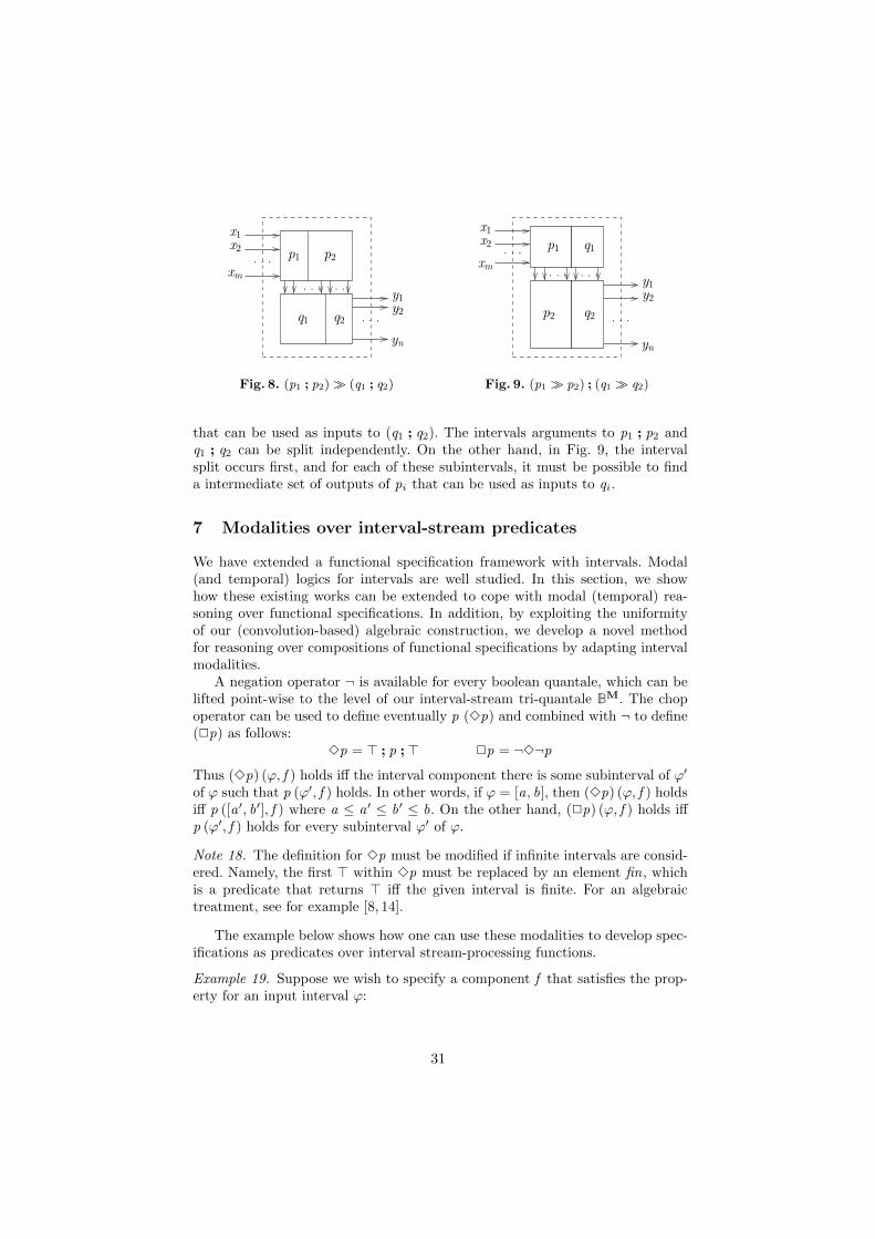
. .
x2
x1
yn
p1
q1
p2
q2
. . .
. . .y2
y1
xm. . .
Fig. 8. (p1 ; p2) >> (q1 ; q2)
y2
x2
x1
. . .xm
p1 q1
yn
y1. . .. . .
q2p2 . . .
Fig. 9. (p1 >> p2) ; (q1 >> q2)
that can be used as inputs to (q1 ; q2). The intervals arguments to p1 ; p2 andq1 ; q2 can be split independently. On the other hand, in Fig. 9, the intervalsplit occurs first, and for each of these subintervals, it must be possible to finda intermediate set of outputs of pi that can be used as inputs to qi .
7 Modalities over interval-stream predicates
We have extended a functional specification framework with intervals. Modal(and temporal) logics for intervals are well studied. In this section, we showhow these existing works can be extended to cope with modal (temporal) rea-soning over functional specifications. In addition, by exploiting the uniformityof our (convolution-based) algebraic construction, we develop a novel methodfor reasoning over compositions of functional specifications by adapting intervalmodalities.
A negation operator ¬ is available for every boolean quantale, which can belifted point-wise to the level of our interval-stream tri-quantale BM. The chopoperator can be used to define eventually p (3p) and combined with ¬ to define(2p) as follows:
3p = > ; p ; > 2p = ¬3¬p
Thus (3p) (', f ) holds i↵ the interval component there is some subinterval of '0
of ' such that p ('0, f ) holds. In other words, if ' = [a, b], then (3p) (', f ) holdsi↵ p ([a 0, b0], f ) where a a 0 b0 b. On the other hand, (2p) (', f ) holds i↵p ('0, f ) holds for every subinterval '0 of '.
Note 18. The definition for 3p must be modified if infinite intervals are consid-ered. Namely, the first > within 3p must be replaced by an element fin, whichis a predicate that returns > i↵ the given interval is finite. For an algebraictreatment, see for example [8, 14].
The example below shows how one can use these modalities to develop spec-ifications as predicates over interval stream-processing functions.
Example 19. Suppose we wish to specify a component f that satisfies the prop-erty for an input interval ':
31
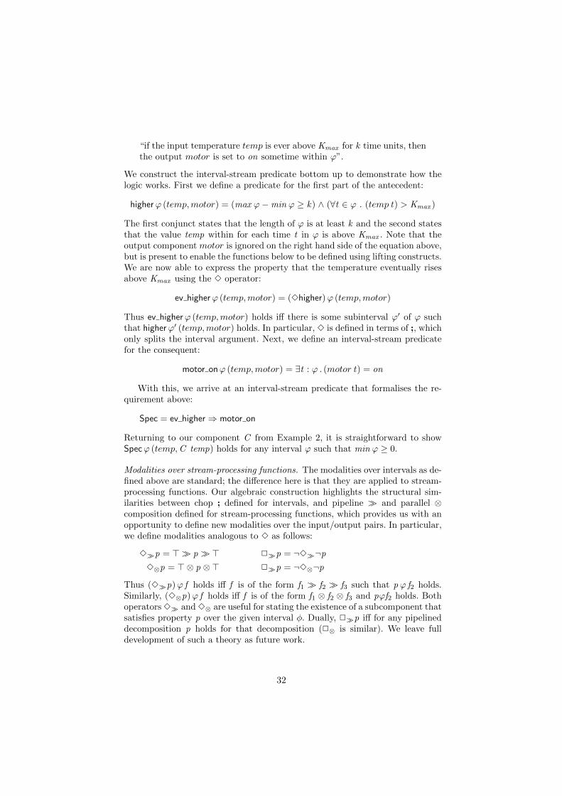
“if the input temperature temp is ever above Kmax for k time units, thenthe output motor is set to on sometime within '”.
We construct the interval-stream predicate bottom up to demonstrate how thelogic works. First we define a predicate for the first part of the antecedent:
higher' (temp, motor) = (max '� min ' � k) ^ (8t 2 ' . (temp t) > Kmax )
The first conjunct states that the length of ' is at least k and the second statesthat the value temp within for each time t in ' is above Kmax . Note that theoutput component motor is ignored on the right hand side of the equation above,but is present to enable the functions below to be defined using lifting constructs.We are now able to express the property that the temperature eventually risesabove Kmax using the 3 operator:
ev higher' (temp, motor) = (3higher)' (temp, motor)
Thus ev higher' (temp, motor) holds i↵ there is some subinterval '0 of ' suchthat higher'0 (temp, motor) holds. In particular, 3 is defined in terms of ;, whichonly splits the interval argument. Next, we define an interval-stream predicatefor the consequent:
motor on' (temp, motor) = 9t : ' . (motor t) = on
With this, we arrive at an interval-stream predicate that formalises the re-quirement above:
Spec = ev higher ) motor on
Returning to our component C from Example 2, it is straightforward to showSpec' (temp,C temp) holds for any interval ' such that min ' � 0.
Modalities over stream-processing functions. The modalities over intervals as de-fined above are standard; the di↵erence here is that they are applied to stream-processing functions. Our algebraic construction highlights the structural sim-ilarities between chop ; defined for intervals, and pipeline >> and parallel ⌦composition defined for stream-processing functions, which provides us with anopportunity to define new modalities over the input/output pairs. In particular,we define modalities analogous to 3 as follows:
3>>p = > >> p >> > 2>>p = ¬3>>¬p
3⌦p = >⌦ p ⌦> 2>>p = ¬3⌦¬p
Thus (3>>p)' f holds i↵ f is of the form f1 >> f2 >> f3 such that p ' f2 holds.Similarly, (3⌦p)' f holds i↵ f is of the form f1 ⌦ f2 ⌦ f3 and p'f2 holds. Bothoperators 3>> and 3⌦ are useful for stating the existence of a subcomponent thatsatisfies property p over the given interval �. Dually, 2>>p i↵ for any pipelineddecomposition p holds for that decomposition (2⌦ is similar). We leave fulldevelopment of such a theory as future work.
32
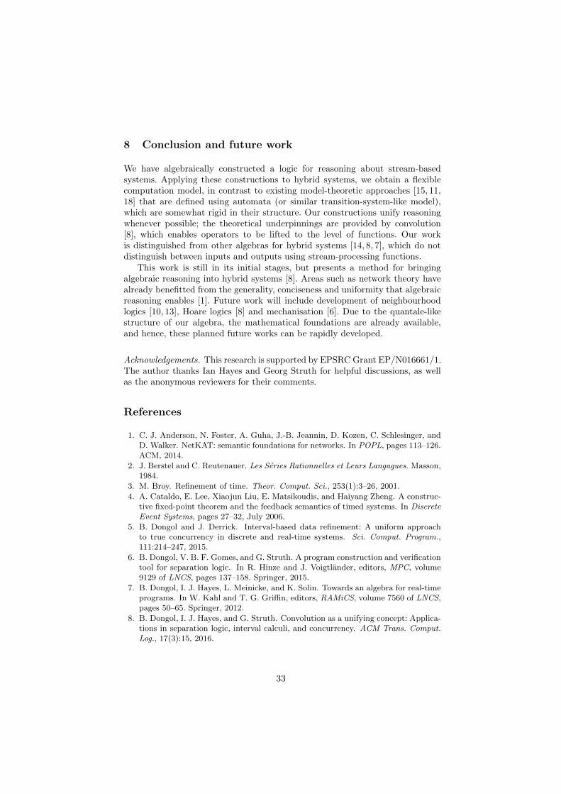
8 Conclusion and future work
We have algebraically constructed a logic for reasoning about stream-basedsystems. Applying these constructions to hybrid systems, we obtain a flexiblecomputation model, in contrast to existing model-theoretic approaches [15, 11,18] that are defined using automata (or similar transition-system-like model),which are somewhat rigid in their structure. Our constructions unify reasoningwhenever possible; the theoretical underpinnings are provided by convolution[8], which enables operators to be lifted to the level of functions. Our workis distinguished from other algebras for hybrid systems [14, 8, 7], which do notdistinguish between inputs and outputs using stream-processing functions.
This work is still in its initial stages, but presents a method for bringingalgebraic reasoning into hybrid systems [8]. Areas such as network theory havealready benefitted from the generality, conciseness and uniformity that algebraicreasoning enables [1]. Future work will include development of neighbourhoodlogics [10, 13], Hoare logics [8] and mechanisation [6]. Due to the quantale-likestructure of our algebra, the mathematical foundations are already available,and hence, these planned future works can be rapidly developed.
Acknowledgements. This research is supported by EPSRC Grant EP/N016661/1.The author thanks Ian Hayes and Georg Struth for helpful discussions, as wellas the anonymous reviewers for their comments.
References
1. C. J. Anderson, N. Foster, A. Guha, J.-B. Jeannin, D. Kozen, C. Schlesinger, andD. Walker. NetKAT: semantic foundations for networks. In POPL, pages 113–126.ACM, 2014.
2. J. Berstel and C. Reutenauer. Les Series Rationnelles et Leurs Langagues. Masson,1984.
3. M. Broy. Refinement of time. Theor. Comput. Sci., 253(1):3–26, 2001.
4. A. Cataldo, E. Lee, Xiaojun Liu, E. Matsikoudis, and Haiyang Zheng. A construc-tive fixed-point theorem and the feedback semantics of timed systems. In DiscreteEvent Systems, pages 27–32, July 2006.
5. B. Dongol and J. Derrick. Interval-based data refinement: A uniform approachto true concurrency in discrete and real-time systems. Sci. Comput. Program.,111:214–247, 2015.
6. B. Dongol, V. B. F. Gomes, and G. Struth. A program construction and verificationtool for separation logic. In R. Hinze and J. Voigtlander, editors, MPC, volume9129 of LNCS, pages 137–158. Springer, 2015.
7. B. Dongol, I. J. Hayes, L. Meinicke, and K. Solin. Towards an algebra for real-timeprograms. In W. Kahl and T. G. Gri�n, editors, RAMiCS, volume 7560 of LNCS,pages 50–65. Springer, 2012.
8. B. Dongol, I. J. Hayes, and G. Struth. Convolution as a unifying concept: Applica-tions in separation logic, interval calculi, and concurrency. ACM Trans. Comput.Log., 17(3):15, 2016.
33
9. M. Droste, W. Kuich, and H. Vogler, editors. Handbook of Weighted Automata.Springer, 2009.
10. V. Goranko, A. Montanari, and G. Sciavicco. A road map of interval temporallogics and duration calculi. Journal of Applied Non-Classical Logics, 14(1-2):9–54,2004.
11. T. A. Henzinger. The theory of hybrid automata. In LICS ’96, pages 278–292,Washington, DC, USA, 1996. IEEE Computer Society.
12. T. Hoare and S. van Staden. In praise of algebra. Formal Asp. Comput., 24(4-6):423–431, 2012.
13. P. Hofner and B. Moller. Algebraic neighbourhood logic. J. Log. Algebr. Program.,76(1):35–59, 2008.
14. P. Hofner and B. Moller. An algebra of hybrid systems. J. Log. Algebr. Program.,78(2):74–97, 2009.
15. N. Lynch, R. Segala, and F. Vaandraager. Hybrid I/O automata. Information andComputation, 185(1):105–157, 2003.
16. B. C. Moszkowski. A complete axiomatization of interval temporal logic withinfinite time. In LICS, pages 241–252, 2000.
17. O. Muller and P. Scholz. Functional specification of real-time and hybrid systems.In O. Maler, editor, HART, volume 1201 of LNCS, pages 273–285. Springer, 1997.
18. M. Ronkko, A. P. Ravn, and K. Sere. Hybrid action systems. Theor. Comput.Sci., 290:937–973, January 2003.
19. C. Zhou and M. R. Hansen. Duration Calculus: A Formal Approach to Real-TimeSystems. EATCS: Monographs in Theoretical Computer Science. Springer, 2004.
34
Automating Time Series Safety Analysisfor Automotive Control Systems in STPA
using Weighted Partial Max-SMT
Shuichi Sato1,2, Shogo Hattori2, Hiroyuki Seki2,Yutaka Inamori1, and Shoji Yuen2
1 Data Analytics Research-Domain,Toyota Central R&D Labs.,Inc., Nagakute, Japan
2 Graduate School of Information Science,Nagoya University, Nagoya, Japan
{shuichi-sato,inamori}@mosk.tytlabs.co.jp{hatsutori,seki,yuen}@sqlab.jp
http://www.tytlabs.co.jp/
Abstract. Recently, Systems-Theoretic Process Analysis (STPA) hasbeen studied for automobile safety analysis. When STPA is used later inthe design phase, significant effort is required to detect causal scenariosof unsafe control actions (UCAs), especially those related to intermit-tent disturbances in multiple signals. We propose a method to automatethis disturbance detection by checking the satisfiability of trace formulasextended with cushion variables. At a state transition, cushion variablevalues are used instead of original variable values to determine the nextstate. A signal disturbance is regarded as assigning different values tovariables and corresponding cushion variables. Specifying the equalitybetween variables and cushion variables as soft clauses, a Weighted Par-tial Max-SMT solver mechanically searches an assignment for a trace tosatisfy the UCA property. We applied the proposed technique to a sim-plified automotive control system to demonstrate some examples of au-tomatic detections of reasonable intermittent multi-signal disturbances.
Keywords: Safety Analysis, Time Series Analysis, Automotive ControlSystems, STPA, State Transition Systems, Trace Formula
1 Introduction
In a variety of fields, such as the aerospace and aeronautics, medicine, and auto-motive industries, system architectures and functionality are becoming increas-ingly complicated. Systems-Theoretic Process Analysis (STPA) [1] [2] has beenproposed as a new safety analysis technique based on a new accident causationmodel, System-Theoretic Accident Model and Process (STAMP), for analyzinghazard and safety issues in complex systems. Some works [3] [4] have demon-strated the advantages of STPA over existing safety analysis techniques such asFault Tree Analysis (FTA) [5], Failure Mode and Effects Analysis (FMEA) [6],
35
2 Automating Time Series Safety Analysis for Automotive Control Systems
and Hazards and Operability Analysis (HAZOP) [7]. STPA has been applied indifferent areas, such as aerospace [8], railroad transportation [9], and medicalresearch [10] [11]. In the automotive field, Hommes [12] proposes to apply STPAto safety analysis compliant with ISO26262, a functional safety standard for roadvehicles.
STPA is a top-down systems engineering approach and incorporates controlsystem theory. It considers both component failures and system interactionsand treats accidents as a control, not a failure, problem. STPA can be appliedduring concept development and throughout the design process. Fig. 1 outlinesthe steps of the STPA procedure. The Control Structure in Fig. 1 comprisesthe components and paths of a control and feedback system. An unsafe controlaction (UCA) is a control action, such as an operation command to an actuator,that leads to a hazard.
Preparation (Step 0)‐Identify Accidents and Hazards‐Construct Control Structure
Step 1: Identify Unsafe Control ActionsStep 2: Identify Causes of Unsafe Control Actions
Fig. 1. STPA procedure
Steps 1 and 2 are carried out with the consideration of a safety engineer,based on guidewords from STPA. Some works [11] point out that examiningthe controller and assessing each feedback in the control path to see whether apath can cause UCAs in Step 2 requires effort, time, and in-depth knowledge. Itis especially difficult to deal with intermittent multi-signal disturbances arisingfrom some undesired factors such as temporal wire disconnections, when weuse STPA in later design phases, because there are an enormous number of timeseries patterns in multiple signals to consider for the thorough STPA application.
In this paper, we focus on the intermittent multi-signal disturbances thatcause UCAs in automobiles. Generally, intermittent signal disturbances are sub-tle; thus, we consider it very useful to automate the analysis on those distur-bances. For this purpose, we present an automating method to check the propertyfor traces of an automotive control system with bounded length. We reduce thereachability (to undesirable states) to the satisfiability problem (abbreviated asSAT) by encoding a given state transition system into a logical formula. Thisapproach is promising because it allows for the utilization of efficient algorithmsand tools (e.g., SAT solver) for judging satisfiability. To this end, we first char-acterize the system as a trace formula [13] [14], whose model is a set of traces,and define the UCA property as a constraint over state variables. In normal sit-uations, the system is supposed to work correctly, where the trace formula withthe UCA property is not satisfied. In the case that an error occurs, some valuesare altered such that they do not satisfy the trace formula but do satisfy the
36
Automating Time Series Safety Analysis for Automotive Control Systems 3
UCA property. Thus, we must describe both the normal and abnormal behaviorof the system and use abnormal behavior caused by multi-signal disturbances asa constraint.
An automotive control system reaches hazardous states when control actionswith incorrect values are provided over a certain period of time. From thoseexperiences, we consider that a UCA expression is required to address time series.To efficiently derive the UCAs caused by fewer incorrect values, we introducean encoding of the model into a formula for acquiring intermittent multi-signalUCA-causing disturbances by limiting the number of failures in the constraints.
We adopt a method for describing the constraints underlying problems anddetecting the corresponding signal disturbances automatically. We introduce newvariables, called cushion variables, that correspond to the original variables andallow a different value assignment from those of the original variables. We define asignal disturbance as the assignment of a different value to a system variable. Thefaulty values of cushion variables cause undesignated transitions, which we modelas UCAs. Considering that the values of an original variable and its cushion areequal in a normal behavior, we explicitly add the equalities between original andcushion variables. By defining a UCA over the cushion variables, assigning faultyvalues to cushion variables may satisfy the UCA violating the equality betweenvariables and cushion variables. The violated equality is regarded as the signaldisturbance that causes the UCA. To obtain the concrete value assignment, wemake the cushion variable equations as soft clauses in the Weighted Partial Max-SMT problem. By adding blocking clauses we obtain a new assignment with asignal disturbance. By repeating this, we can enumerate all signal disturbancesto cause the UCA.
The main contribution of this paper is the proposal of a method for reduc-ing the problem of finding UCA-causing multi-signal disturbances in STPA tothe problem of checking the satisfiability of the trace formula extended withcushion variables. The proposed method can automate the process of obtainingintermittent multi-signal disturbances using a Weighted Partial Max-SMT solverand provide detailed design support to STPA safety analysis.
The remainder of this paper is organized as follows. Section 2 explains howto model the problem of acquiring UCA-causing multi-signal patterns. Section3 presents a method for acquiring intermittent multi-signal disturbances usinga Weighted Partial Max-SMT. Section 4 describes case studies that apply ourmethod to a simplified automotive control system with cruise control, and Sec-tion 5 discusses our conclusions and outlines future work.
2 Behavioral Constraints
In this section, we describe the construction of a system model for finding the in-termittent multi-signal disturbance set that causes UCAs with Weighted PartialMax-SMT. The model consists of four parts: a trace formula expressing systembehavior, the UCA property, signal disturbance possibilities, and intermittent
37
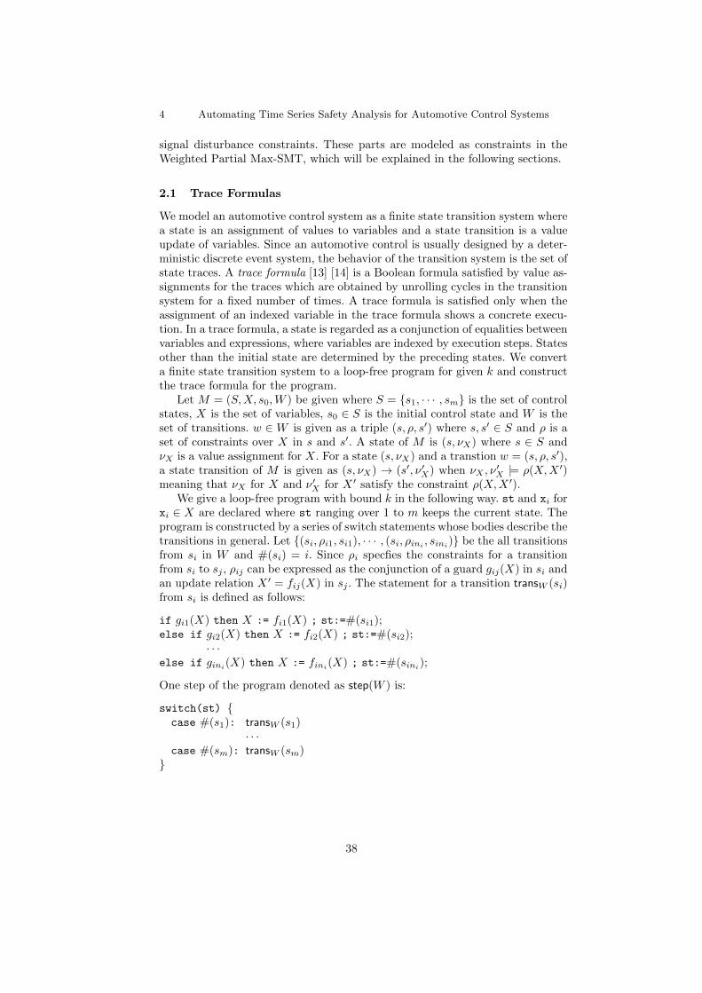
4 Automating Time Series Safety Analysis for Automotive Control Systems
signal disturbance constraints. These parts are modeled as constraints in theWeighted Partial Max-SMT, which will be explained in the following sections.
2.1 Trace Formulas
We model an automotive control system as a finite state transition system wherea state is an assignment of values to variables and a state transition is a valueupdate of variables. Since an automotive control is usually designed by a deter-ministic discrete event system, the behavior of the transition system is the set ofstate traces. A trace formula [13] [14] is a Boolean formula satisfied by value as-signments for the traces which are obtained by unrolling cycles in the transitionsystem for a fixed number of times. A trace formula is satisfied only when theassignment of an indexed variable in the trace formula shows a concrete execu-tion. In a trace formula, a state is regarded as a conjunction of equalities betweenvariables and expressions, where variables are indexed by execution steps. Statesother than the initial state are determined by the preceding states. We converta finite state transition system to a loop-free program for given k and constructthe trace formula for the program.
Let M = (S, X, s0, W ) be given where S = {s1, · · · , sm} is the set of controlstates, X is the set of variables, s0 2 S is the initial control state and W is theset of transitions. w 2 W is given as a triple (s, Ω, s0) where s, s0 2 S and Ω is aset of constraints over X in s and s0. A state of M is (s, ∫X) where s 2 S and∫X is a value assignment for X. For a state (s, ∫X) and a transtion w = (s, Ω, s0),a state transition of M is given as (s, ∫X) ! (s0, ∫0X) when ∫X , ∫0X |= Ω(X,X 0)meaning that ∫X for X and ∫0X for X 0 satisfy the constraint Ω(X,X 0).
We give a loop-free program with bound k in the following way. st and xi forxi 2 X are declared where st ranging over 1 to m keeps the current state. Theprogram is constructed by a series of switch statements whose bodies describe thetransitions in general. Let {(si, Ωi1, si1), · · · , (si, Ωini , sini)} be the all transitionsfrom si in W and #(si) = i. Since Ωi specfies the constraints for a transitionfrom si to sj , Ωij can be expressed as the conjunction of a guard gij(X) in si andan update relation X 0 = fij(X) in sj . The statement for a transition transW (si)from si is defined as follows:
if gi1(X) then X := fi1(X) ; st:=#(si1);else if gi2(X) then X := fi2(X) ; st:=#(si2);
· · ·else if gini(X) then X := fini(X) ; st:=#(sini);
One step of the program denoted as step(W ) is:
switch(st) {case #(s1): transW (s1)
· · ·case #(sm): transW (sm)
}
38
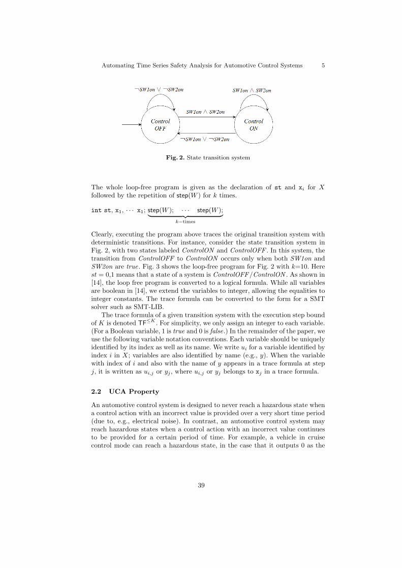
Automating Time Series Safety Analysis for Automotive Control Systems 5
Fig. 2. State transition system
The whole loop-free program is given as the declaration of st and xi for Xfollowed by the repetition of step(W ) for k times.
int st, x1, · · · x1; step(W ); · · · step(W );| {z }k°times
Clearly, executing the program above traces the original transition system withdeterministic transitions. For instance, consider the state transition system inFig. 2, with two states labeled ControlON and ControlOFF . In this system, thetransition from ControlOFF to ControlON occurs only when both SW1on andSW2on are true. Fig. 3 shows the loop-free program for Fig. 2 with k=10. Herest = 0,1 means that a state of a system is ControlOFF/ControlON . As shown in[14], the loop free program is converted to a logical formula. While all variablesare boolean in [14], we extend the variables to integer, allowing the equalities tointeger constants. The trace formula can be converted to the form for a SMTsolver such as SMT-LIB.
The trace formula of a given transition system with the execution step boundof K is denoted TF∑K . For simplicity, we only assign an integer to each variable.(For a Boolean variable, 1 is true and 0 is false.) In the remainder of the paper, weuse the following variable notation conventions. Each variable should be uniquelyidentified by its index as well as its name. We write ui for a variable identified byindex i in X; variables are also identified by name (e.g., y). When the variablewith index of i and also with the name of y appears in a trace formula at stepj, it is written as ui,j or yj , where ui,j or yj belongs to xj in a trace formula.
2.2 UCA Property
An automotive control system is designed to never reach a hazardous state whena control action with an incorrect value is provided over a very short time period(due to, e.g., electrical noise). In contrast, an automotive control system mayreach hazardous states when a control action with an incorrect value continuesto be provided for a certain period of time. For example, a vehicle in cruisecontrol mode can reach a hazardous state, in the case that it outputs 0 as the
39
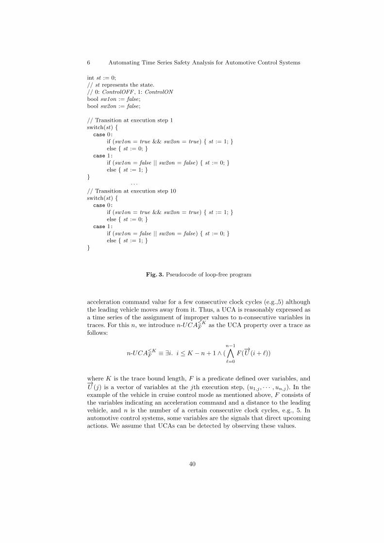
6 Automating Time Series Safety Analysis for Automotive Control Systems
int st := 0;// st represents the state.// 0: ControlOFF , 1: ControlONbool sw1on := false;bool sw2on := false;
// Transition at execution step 1switch(st) {case 0:
if (sw1on = true && sw2on = true) { st := 1; }else { st := 0; }
case 1:if (sw1on = false || sw2on = false) { st := 0; }else { st := 1; }
}· · ·
// Transition at execution step 10switch(st) {case 0:
if (sw1on = true && sw2on = true) { st := 1; }else { st := 0; }
case 1:if (sw1on = false || sw2on = false) { st := 0; }else { st := 1; }
}
Fig. 3. Pseudocode of loop-free program
acceleration command value for a few consecutive clock cycles (e.g.,5) althoughthe leading vehicle moves away from it. Thus, a UCA is reasonably expressed asa time series of the assignment of improper values to n-consecutive variables intraces. For this n, we introduce n-UCA∑K
F as the UCA property over a trace asfollows:
n-UCA∑KF ¥ 9i. i ∑ K ° n + 1 ^ (
n°1
`=0
F (°!U (i + `))
where K is the trace bound length, F is a predicate defined over variables, and°!U (j) is a vector of variables at the jth execution step, (u1,j , · · · , un,j). In theexample of the vehicle in cruise control mode as mentioned above, F consists ofthe variables indicating an acceleration command and a distance to the leadingvehicle, and n is the number of a certain consecutive clock cycles, e.g., 5. Inautomotive control systems, some variables are the signals that direct upcomingactions. We assume that UCAs can be detected by observing these values.
40
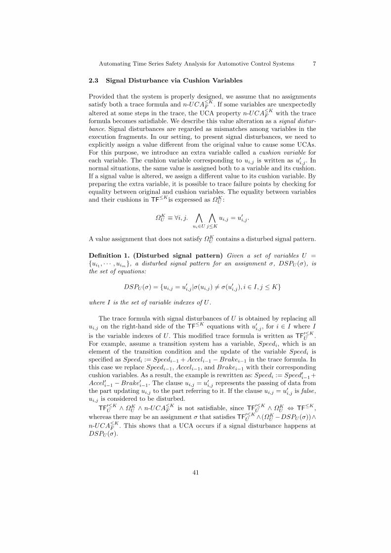
Automating Time Series Safety Analysis for Automotive Control Systems 7
2.3 Signal Disturbance via Cushion Variables
Provided that the system is properly designed, we assume that no assignmentssatisfy both a trace formula and n-UCA∑K
F . If some variables are unexpectedly
altered at some steps in the trace, the UCA property n-UCA∑KF with the trace
formula becomes satisfiable. We describe this value alteration as a signal distur-bance. Signal disturbances are regarded as mismatches among variables in theexecution fragments. In our setting, to present signal disturbances, we need toexplicitly assign a value different from the original value to cause some UCAs.For this purpose, we introduce an extra variable called a cushion variable foreach variable. The cushion variable corresponding to ui,j is written as u0
i,j . Innormal situations, the same value is assigned both to a variable and its cushion.If a signal value is altered, we assign a different value to its cushion variable. Bypreparing the extra variable, it is possible to trace failure points by checking forequality between original and cushion variables. The equality between variablesand their cushions in TF∑K is expressed as ≠K
U :
≠KU ¥ 8i, j.
^
ui2U
^
j∑K
ui,j = u0i,j .
A value assignment that does not satisfy ≠KU contains a disturbed signal pattern.
Definition 1. (Disturbed signal pattern) Given a set of variables U ={ui1 , · · · , uim}, a disturbed signal pattern for an assignment æ, DSPU (æ), isthe set of equations:
DSPU (æ) = {ui,j = u0i,j |æ(ui,j) 6= æ(u0
i,j), i 2 I, j ∑ K}
where I is the set of variable indexes of U .
The trace formula with signal disturbances of U is obtained by replacing allui,j on the right-hand side of the TF∑K equations with u0
i,j , for i 2 I where I
is the variable indexes of U . This modified trace formula is written as TF0∑KU .
For example, assume a transition system has a variable, Speedi, which is anelement of the transition condition and the update of the variable Speedi isspecified as Speedi := Speedi°1 + Acceli°1 ° Brakei°1 in the trace formula. Inthis case we replace Speedi°1, Acceli°1, and Brakei°1 with their correspondingcushion variables. As a result, the example is rewritten as: Speedi := Speed0
i°1+Accel0i°1 °Brake0i°1. The clause ui,j = u0
i,j represents the passing of data fromthe part updating ui,j to the part referring to it. If the clause ui,j = u0
i,j is false,ui,j is considered to be disturbed.
TF0∑KU ^ ≠K
U ^ n-UCA∑KF is not satisfiable, since TF0∑K
U ^ ≠KU , TF∑K ,
whereas there may be an assignment æ that satisfies TF0∑KU ^(≠K
U °DSPU (æ))^n-UCA∑K
F . This shows that a UCA occurs if a signal disturbance happens atDSPU (æ).
41
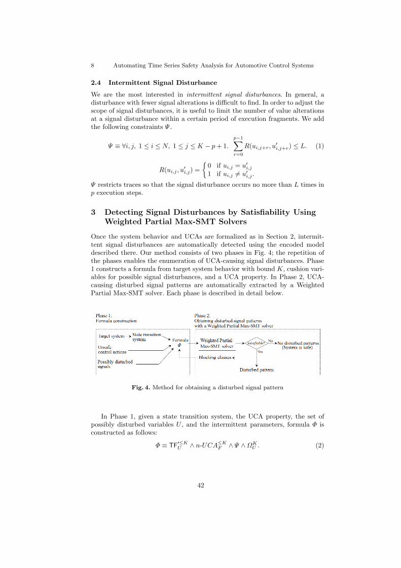
8 Automating Time Series Safety Analysis for Automotive Control Systems
2.4 Intermittent Signal Disturbance
We are the most interested in intermittent signal disturbances. In general, adisturbance with fewer signal alterations is difficult to find. In order to adjust thescope of signal disturbances, it is useful to limit the number of value alterationsat a signal disturbance within a certain period of execution fragments. We addthe following constraints ™ .
™ ¥ 8i, j, 1 ∑ i ∑ N, 1 ∑ j ∑ K ° p + 1.
p°1X
r=0
R(ui,j+r, u0i,j+r) ∑ L. (1)
R(ui,j , u0i,j) =
Ω0 if ui,j = u0
i,j
1 if ui,j 6= u0i,j .
™ restricts traces so that the signal disturbance occurs no more than L times inp execution steps.
3 Detecting Signal Disturbances by Satisfiability UsingWeighted Partial Max-SMT Solvers
Once the system behavior and UCAs are formalized as in Section 2, intermit-tent signal disturbances are automatically detected using the encoded modeldescribed there. Our method consists of two phases in Fig. 4; the repetition ofthe phases enables the enumeration of UCA-causing signal disturbances. Phase1 constructs a formula from target system behavior with bound K, cushion vari-ables for possible signal disturbances, and a UCA property. In Phase 2, UCA-causing disturbed signal patterns are automatically extracted by a WeightedPartial Max-SMT solver. Each phase is described in detail below.
Fig. 4. Method for obtaining a disturbed signal pattern
In Phase 1, given a state transition system, the UCA property, the set ofpossibly disturbed variables U , and the intermittent parameters, formula © isconstructed as follows:
© ¥ TF0∑KU ^ n-UCA∑K
F ^ ™ ^≠KU . (2)
42
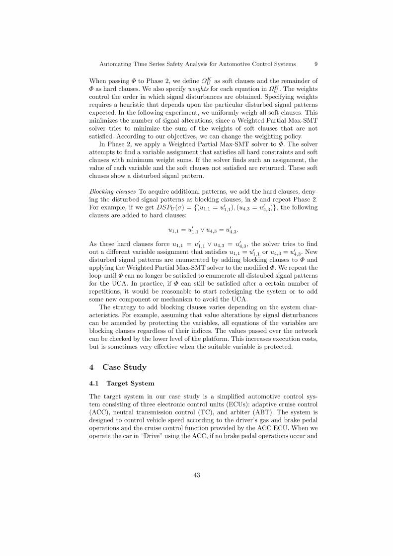
Automating Time Series Safety Analysis for Automotive Control Systems 9
When passing © to Phase 2, we define ≠KU as soft clauses and the remainder of
© as hard clauses. We also specify weights for each equation in ≠KU . The weights
control the order in which signal disturbances are obtained. Specifying weightsrequires a heuristic that depends upon the particular disturbed signal patternsexpected. In the following experiment, we uniformly weigh all soft clauses. Thisminimizes the number of signal alterations, since a Weighted Partial Max-SMTsolver tries to minimize the sum of the weights of soft clauses that are notsatisfied. According to our objectives, we can change the weighting policy.
In Phase 2, we apply a Weighted Partial Max-SMT solver to ©. The solverattempts to find a variable assignment that satisfies all hard constraints and softclauses with minimum weight sums. If the solver finds such an assignment, thevalue of each variable and the soft clauses not satisfied are returned. These softclauses show a disturbed signal pattern.
Blocking clauses To acquire additional patterns, we add the hard clauses, deny-ing the disturbed signal patterns as blocking clauses, in © and repeat Phase 2.For example, if we get DSPU (æ) = {(u1,1 = u0
1,1), (u4,3 = u04,3)}, the following
clauses are added to hard clauses:
u1,1 = u01,1 _ u4,3 = u0
4,3.
As these hard clauses force u1,1 = u01,1 _ u4,3 = u0
4,3, the solver tries to findout a different variable assignment that satisfies u1,1 = u0
1,1 or u4,3 = u04,3. New
disturbed signal patterns are enumerated by adding blocking clauses to © andapplying the Weighted Partial Max-SMT solver to the modified ©. We repeat theloop until © can no longer be satisfied to enumerate all distrubed signal patternsfor the UCA. In practice, if © can still be satisfied after a certain number ofrepetitions, it would be reasonable to start redesigning the system or to addsome new component or mechanism to avoid the UCA.
The strategy to add blocking clauses varies depending on the system char-acteristics. For example, assuming that value alterations by signal disturbancescan be amended by protecting the variables, all equations of the variables areblocking clauses regardless of their indices. The values passed over the networkcan be checked by the lower level of the platform. This increases execution costs,but is sometimes very effective when the suitable variable is protected.
4 Case Study
4.1 Target System
The target system in our case study is a simplified automotive control sys-tem consisting of three electronic control units (ECUs): adaptive cruise control(ACC), neutral transmission control (TC), and arbiter (ABT). The system isdesigned to control vehicle speed according to the driver’s gas and brake pedaloperations and the cruise control function provided by the ACC ECU. When weoperate the car in “Drive” using the ACC, if no brake pedal operations occur and
43
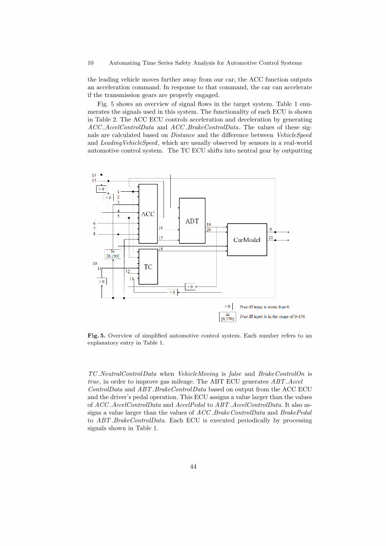
10 Automating Time Series Safety Analysis for Automotive Control Systems
the leading vehicle moves further away from our car, the ACC function outputsan acceleration command. In response to that command, the car can accelerateif the transmission gears are properly engaged.
Fig. 5 shows an overview of signal flows in the target system. Table 1 enu-merates the signals used in this system. The functionality of each ECU is shownin Table 2. The ACC ECU controls acceleration and deceleration by generatingACC AccelControlData and ACC BrakeControlData. The values of these sig-nals are calculated based on Distance and the difference between VehicleSpeedand LeadingVehicleSpeed , which are usually observed by sensors in a real-worldautomotive control system. The TC ECU shifts into neutral gear by outputting
Fig. 5. Overview of simplified automotive control system. Each number refers to anexplanatory entry in Table 1.
TC NeutralControlData when VehicleMoving is false and BrakeControlOn istrue, in order to improve gas mileage. The ABT ECU generates ABT AccelControlData and ABT BrakeControlData based on output from the ACC ECUand the driver’s pedal operation. This ECU assigns a value larger than the valuesof ACC AccelControlData and AccelPedal to ABT AccelControlData. It also as-signs a value larger than the values of ACC BrakeControlData and BrakePedalto ABT BrakeControlData. Each ECU is executed periodically by processingsignals shown in Table 1.
44
Automating Time Series Safety Analysis for Automotive Control Systems 11
Table 1. Target system signals
No. Name Type Meaning
1 IGSWOn bool True iff Ignition switch is on2 RadarCruiseSWOn bool True iff ACC main switch is on3 VehicleSpeedOK bool True iff vehicle speed is in [0,150]4 AccelPedalOn bool True iff gas pedal is stepped on5 BrakePedalOn bool True iff brake pedal is stepped on6 ShiftRange int Shift range(°2:P °1:R 0:N 1–5:D)7 Fail ACC bool True iff ACC fails8 LeadingVehicleSpeed int Speed of leading vehicle9 Distance int Distance to leading vehicle10 Fail TC bool True iff the TC fails11 VehicleMoving bool True iff vehicle is moving12 ABT AccelControlOn bool True iff ABT AccelControlData > 013 ABT BrakeControlOn bool True iff ABT BrakeControlData > 014 AccelPedal int Amount by which gas pedal is depressed15 BrakePedal int Amount by which brake pedal is depressed16 ACC AccelControlData int Acceleration control value from ACC ECU17 ACC BrakeControlData int Braking control value from ACC ECU18 TC NeutralControlData bool Neutral control value from TC ECU19 ABT AccelControlData int Integrated acceleration control value20 ABT BrakeControlData int Integrated braking control value21 VehicleSpeed int Speed of vehicle
Table 2. ECUs in target system
Name Function
ACC Controls acceleration and deceleration in accordance with leading vehicleTC Shifts into neutral gear during brief stops in order to improve
gas mileageABT Arbitrates multiple control requests
The CarModel in Fig. 5 shows the physical behavior of the vehicle. It gen-erates VehicleSpeed based on ABT AccelControlData, ABT BrakeControlData,TC NeutralControlData, previous VehicleSpeed , etc. It also outputs Distance si-multaneously calculated based on previous Distance, LeadingVehicleSpeed , andVehicle Speed . Linear arithmetic, comparison, and conditional branch opera-tions are included in this model. The control logic in the ACC ECU includesthe comparison between VehicleSpeed and LeadingVehicleSpeed . The CarModelhas linear arithmetic functions to calculate VehicleSpeed . ACC and TC ECUscontain state transitions with Boolean guard conditions.
45
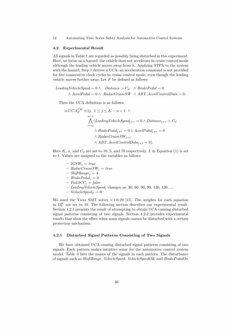
12 Automating Time Series Safety Analysis for Automotive Control Systems
4.2 Experimental Result
All signals in Table 1 are regarded as possibly being disturbed in this experiment.Here, we focus on a hazard: the vehicle does not accelerate in cruise control modealthough the leading vehicle moves away from it. Applying STPA to the systemwith the hazard, Step 1 derives a UCA: an acceleration command is not providedfor five consecutive clock cycles in cruise control mode, even though the leadingvehicle moves further away. Let F be defined as follows:
LeadingVehicleSpeed = 0 ^ Distance > Cd ^ BrakePedal = 0
^ AccelPedal = 0 ^ RadarCruiseSW ^ ABT AccelControlData = 0.
Then the UCA definition is as follows:
n-UCA∑KF ¥9j. 1 ∑ j ∑ K ° n + 1 ^
n°1
r=0
(LeadingVehicleSpeedj+r = 0 ^ Distancej+r > Cd
^ BrakePedalj+r = 0 ^ AccelPedalj+r = 0
^ RadarCruiseSWj+r
^ ABT AccelControlDataj+r = 0).
Here K, n, and Cd are set to 10, 5, and 70 respectively. L in Equation (1) is setto 1. Values are assigned to the variables as follows:
– IGSWj = true– RadarCruiseSWj = true– ShiftRangej = 4– BrakePedalj = 0– FailACCj = false– LeadingVehicleSpeedj changes as: 30, 60, 90, 90, 120, 120, ...– VehicleSpeed0 = 0
We used the Yices SMT solver v.1.0.29 [15]. The weights for each equationin ≠K
U are set to 10. The following section describes our experimental result.Section 4.2.1 presents the result of attempting to obtain UCA-causing disturbedsignal patterns consisting of two signals. Section 4.2.2 provides experimentalresults that show the effect when some signals cannot be disturbed with a certainprotection mechanism.
4.2.1 Disturbed Signal Patterns Consisting of Two Signals
We have obtained UCA-causing disturbed signal patterns consisting of twosignals. Each pattern makes intuitive sense for the automotive control systemmodel. Table 3 lists the names of the signals in each pattern. The disturbanceof signals such as ShiftRange, VehicleSpeed , VehicleSpeedOK and BrakePedalOn
46
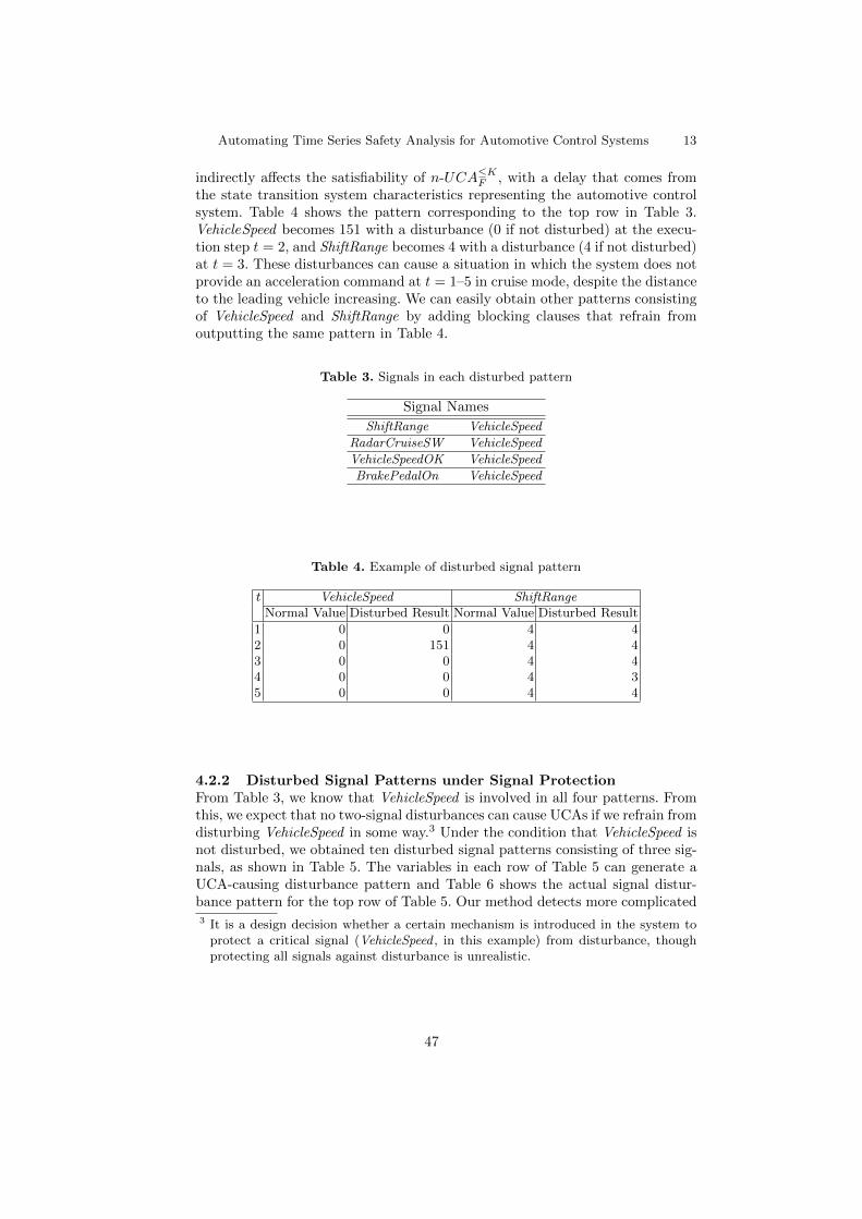
Automating Time Series Safety Analysis for Automotive Control Systems 13
indirectly affects the satisfiability of n-UCA∑KF , with a delay that comes from
the state transition system characteristics representing the automotive controlsystem. Table 4 shows the pattern corresponding to the top row in Table 3.VehicleSpeed becomes 151 with a disturbance (0 if not disturbed) at the execu-tion step t = 2, and ShiftRange becomes 4 with a disturbance (4 if not disturbed)at t = 3. These disturbances can cause a situation in which the system does notprovide an acceleration command at t = 1–5 in cruise mode, despite the distanceto the leading vehicle increasing. We can easily obtain other patterns consistingof VehicleSpeed and ShiftRange by adding blocking clauses that refrain fromoutputting the same pattern in Table 4.
Table 3. Signals in each disturbed pattern
Signal Names
ShiftRange VehicleSpeed
RadarCruiseSW VehicleSpeed
VehicleSpeedOK VehicleSpeed
BrakePedalOn VehicleSpeed
Table 4. Example of disturbed signal pattern
t VehicleSpeed ShiftRangeNormal Value Disturbed Result Normal Value Disturbed Result
1 0 0 4 42 0 151 4 43 0 0 4 44 0 0 4 35 0 0 4 4
4.2.2 Disturbed Signal Patterns under Signal ProtectionFrom Table 3, we know that VehicleSpeed is involved in all four patterns. Fromthis, we expect that no two-signal disturbances can cause UCAs if we refrain fromdisturbing VehicleSpeed in some way.3 Under the condition that VehicleSpeed isnot disturbed, we obtained ten disturbed signal patterns consisting of three sig-nals, as shown in Table 5. The variables in each row of Table 5 can generate aUCA-causing disturbance pattern and Table 6 shows the actual signal distur-bance pattern for the top row of Table 5. Our method detects more complicated3 It is a design decision whether a certain mechanism is introduced in the system to
protect a critical signal (VehicleSpeed , in this example) from disturbance, thoughprotecting all signals against disturbance is unrealistic.
47

14 Automating Time Series Safety Analysis for Automotive Control Systems
time series patterns than those with two signals. The computation time to ob-tain the pattern in Table 6 is 1.83 seconds on a machine with an Intel Corei5-3470 3.20GHz CPU, 6.00GB RAM, and Microsoft Windows 7 Professional.Per Table 5, LeadingVehicleSpeed is a key in patterns consisting of three signals.Any three-signal disturbance cannot cause UCAs if we refrain from disturbing ofVehicleSpeed and LeadingVehicleSpeed . This fact was verified by adding a block-ing clause preventing disturbances to VehicleSpeed and LeadingVehicleSpeed .
Table 5. Signals in each disturbed signal pattern
Signal Names
RadarCruiseSW LeadingVehicleSpeed ACC AccelControlData
RadarCruiseSW ShiftRange LeadingVehicleSpeed
ShiftRange LeadingVehicleSpeed ACC AccelControlData
RadarCruiseSW VehicleSpeedOK LeadingVehicleSpeed
VehicleSpeedOK LeadingVehicleSpeed ACC AccelControlData
RadarCruiseSW BrakePedalOn LeadingVehicleSpeed
VehicleSpeedOK ShiftRange LeadingVehicleSpeed
VehicleSpeedOK BrakePedalOn LeadingVehicleSpeed
BrakePedalOn LeadingVehicleSpeed ACC AccelControlData
BrakePedalOn ShiftRange LeadingVehicleSpeed
Table 6. Example of disturbed signal pattern
t RadarCruiseSW LeadingVehicleSpeed ACC AccelControlDataNormal Value Disturbed Result Normal Value Disturbed Result Normal Value Disturbed Result
1 on on 30 30 0 02 on on 60 °21 0 03 on off 90 90 0 04 on on 90 90 0 05 on on 120 120 280 °1
Note that for two-signal disturbances, the total possible number of value pairsfor two signals is 840, even if each signal is binary; for three-signal disturbances,the total number is greater than 10,000. Hence, it is difficult to enumerate UCAsby hand, even for short time series.
5 Conclusion
We focused on STPA safety analysis and presented an automating method toidentify the faulty behavior by signal disturbances that causes UCAs in auto-motive control systems using Weighted Partial Max-SMT solvers. Our method
48
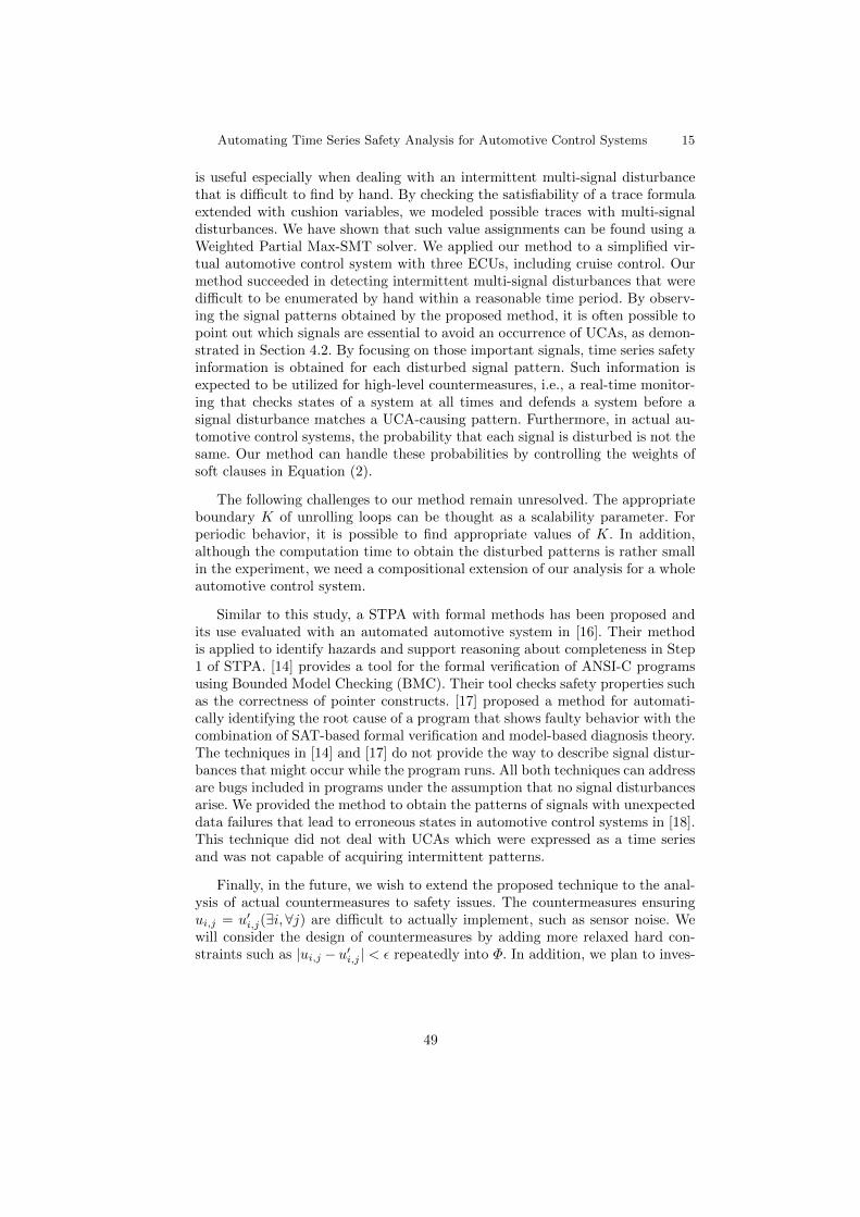
Automating Time Series Safety Analysis for Automotive Control Systems 15
is useful especially when dealing with an intermittent multi-signal disturbancethat is difficult to find by hand. By checking the satisfiability of a trace formulaextended with cushion variables, we modeled possible traces with multi-signaldisturbances. We have shown that such value assignments can be found using aWeighted Partial Max-SMT solver. We applied our method to a simplified vir-tual automotive control system with three ECUs, including cruise control. Ourmethod succeeded in detecting intermittent multi-signal disturbances that weredifficult to be enumerated by hand within a reasonable time period. By observ-ing the signal patterns obtained by the proposed method, it is often possible topoint out which signals are essential to avoid an occurrence of UCAs, as demon-strated in Section 4.2. By focusing on those important signals, time series safetyinformation is obtained for each disturbed signal pattern. Such information isexpected to be utilized for high-level countermeasures, i.e., a real-time monitor-ing that checks states of a system at all times and defends a system before asignal disturbance matches a UCA-causing pattern. Furthermore, in actual au-tomotive control systems, the probability that each signal is disturbed is not thesame. Our method can handle these probabilities by controlling the weights ofsoft clauses in Equation (2).
The following challenges to our method remain unresolved. The appropriateboundary K of unrolling loops can be thought as a scalability parameter. Forperiodic behavior, it is possible to find appropriate values of K. In addition,although the computation time to obtain the disturbed patterns is rather smallin the experiment, we need a compositional extension of our analysis for a wholeautomotive control system.
Similar to this study, a STPA with formal methods has been proposed andits use evaluated with an automated automotive system in [16]. Their methodis applied to identify hazards and support reasoning about completeness in Step1 of STPA. [14] provides a tool for the formal verification of ANSI-C programsusing Bounded Model Checking (BMC). Their tool checks safety properties suchas the correctness of pointer constructs. [17] proposed a method for automati-cally identifying the root cause of a program that shows faulty behavior with thecombination of SAT-based formal verification and model-based diagnosis theory.The techniques in [14] and [17] do not provide the way to describe signal distur-bances that might occur while the program runs. All both techniques can addressare bugs included in programs under the assumption that no signal disturbancesarise. We provided the method to obtain the patterns of signals with unexpecteddata failures that lead to erroneous states in automotive control systems in [18].This technique did not deal with UCAs which were expressed as a time seriesand was not capable of acquiring intermittent patterns.
Finally, in the future, we wish to extend the proposed technique to the anal-ysis of actual countermeasures to safety issues. The countermeasures ensuringui,j = u0
i,j(9i,8j) are difficult to actually implement, such as sensor noise. Wewill consider the design of countermeasures by adding more relaxed hard con-straints such as |ui,j ° u0
i,j | < ≤ repeatedly into ©. In addition, we plan to inves-
49
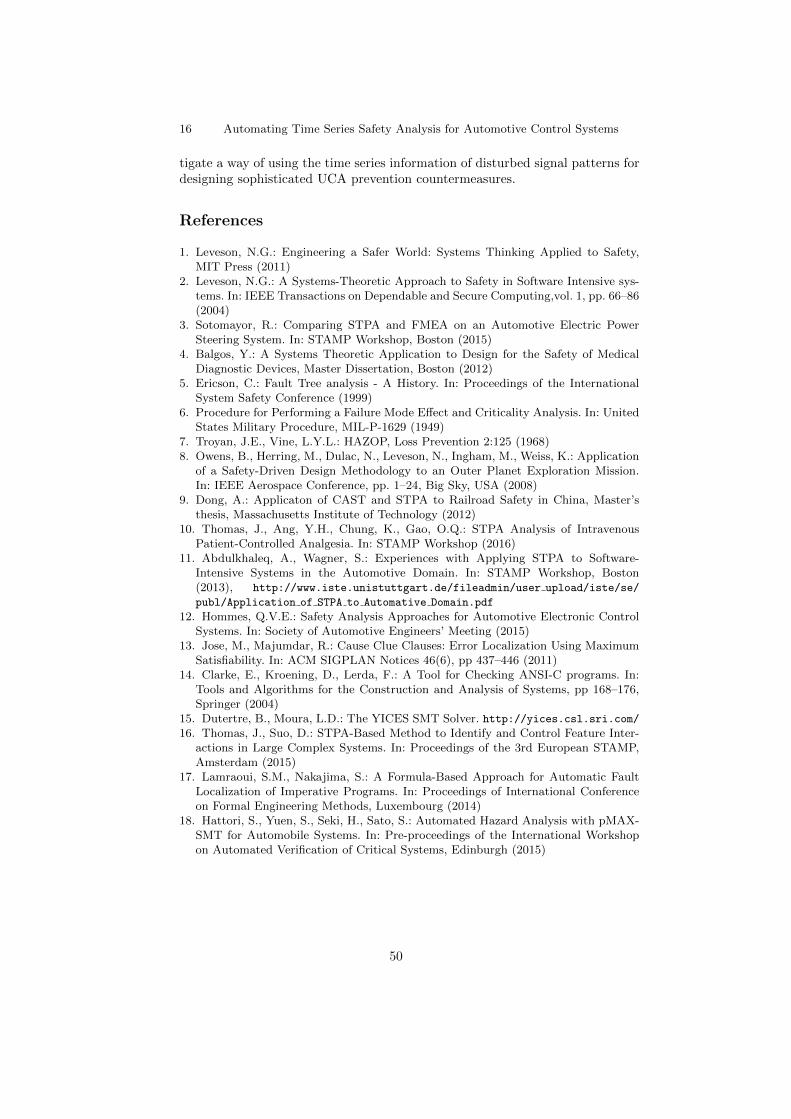
16 Automating Time Series Safety Analysis for Automotive Control Systems
tigate a way of using the time series information of disturbed signal patterns fordesigning sophisticated UCA prevention countermeasures.
References
1. Leveson, N.G.: Engineering a Safer World: Systems Thinking Applied to Safety,MIT Press (2011)
2. Leveson, N.G.: A Systems-Theoretic Approach to Safety in Software Intensive sys-tems. In: IEEE Transactions on Dependable and Secure Computing,vol. 1, pp. 66–86(2004)
3. Sotomayor, R.: Comparing STPA and FMEA on an Automotive Electric PowerSteering System. In: STAMP Workshop, Boston (2015)
4. Balgos, Y.: A Systems Theoretic Application to Design for the Safety of MedicalDiagnostic Devices, Master Dissertation, Boston (2012)
5. Ericson, C.: Fault Tree analysis - A History. In: Proceedings of the InternationalSystem Safety Conference (1999)
6. Procedure for Performing a Failure Mode Effect and Criticality Analysis. In: UnitedStates Military Procedure, MIL-P-1629 (1949)
7. Troyan, J.E., Vine, L.Y.L.: HAZOP, Loss Prevention 2:125 (1968)8. Owens, B., Herring, M., Dulac, N., Leveson, N., Ingham, M., Weiss, K.: Application
of a Safety-Driven Design Methodology to an Outer Planet Exploration Mission.In: IEEE Aerospace Conference, pp. 1–24, Big Sky, USA (2008)
9. Dong, A.: Applicaton of CAST and STPA to Railroad Safety in China, Master’sthesis, Massachusetts Institute of Technology (2012)
10. Thomas, J., Ang, Y.H., Chung, K., Gao, O.Q.: STPA Analysis of IntravenousPatient-Controlled Analgesia. In: STAMP Workshop (2016)
11. Abdulkhaleq, A., Wagner, S.: Experiences with Applying STPA to Software-Intensive Systems in the Automotive Domain. In: STAMP Workshop, Boston(2013), http://www.iste.unistuttgart.de/fileadmin/user upload/iste/se/
publ/Application of STPA to Automative Domain.pdf
12. Hommes, Q.V.E.: Safety Analysis Approaches for Automotive Electronic ControlSystems. In: Society of Automotive Engineers’ Meeting (2015)
13. Jose, M., Majumdar, R.: Cause Clue Clauses: Error Localization Using MaximumSatisfiability. In: ACM SIGPLAN Notices 46(6), pp 437–446 (2011)
14. Clarke, E., Kroening, D., Lerda, F.: A Tool for Checking ANSI-C programs. In:Tools and Algorithms for the Construction and Analysis of Systems, pp 168–176,Springer (2004)
15. Dutertre, B., Moura, L.D.: The YICES SMT Solver. http://yices.csl.sri.com/16. Thomas, J., Suo, D.: STPA-Based Method to Identify and Control Feature Inter-
actions in Large Complex Systems. In: Proceedings of the 3rd European STAMP,Amsterdam (2015)
17. Lamraoui, S.M., Nakajima, S.: A Formula-Based Approach for Automatic FaultLocalization of Imperative Programs. In: Proceedings of International Conferenceon Formal Engineering Methods, Luxembourg (2014)
18. Hattori, S., Yuen, S., Seki, H., Sato, S.: Automated Hazard Analysis with pMAX-SMT for Automobile Systems. In: Pre-proceedings of the International Workshopon Automated Verification of Critical Systems, Edinburgh (2015)
50
Uniform Modeling of Railway Operations
Eduard Kamburjan and Reiner Hahnle
Department of Computer Science, TU Darmstadt, Germany{kamburjan,haehnle}@cs.tu-darmstadt.de
Abstract. We present a comprehensive model of railway operationswritten in the abstract behavioral specification (ABS) language. Themodel is based on specifications taken from the rulebooks of DeutscheBahn AG. It is statically analyzable and executable, hence allows to usestatic and dynamic analysis within one and the same formalism. We areable to combine aspects of micro- and macroscopic modeling and pro-vide a way to inspect changes in the rulebooks. We illustrate the staticanalysis capability by a safety analysis based on invariant reasoning thatonly relies on assumptions about the underlying railway infrastructureinstead of explicitly exploring the state space. A concrete infrastructurelayout and train schedule can be used as input to the model to examinedynamic properties such as delays. We illustrate the capability for dy-namic analysis by demonstrating the e↵ect that di↵erent ways of dealingwith faulty signals have on delays.
1 Introduction
Railway systems are a domain where formal modeling of systems and formalanalysis methods are generally accepted by industry and partially required bycertification authorities [3]. Therefore, the railway domain is an active and im-portant area of applied research in formal methods.
Models of railways can be classified according to their level of abstraction andtheir intended degree of analyzability. Regarding the abstraction level, modelingapproaches tend to be either microscopic or macroscopic. The former focus onmodeling a local part of a railway network, e.g., a few train station to be asprecise enough to examine local and detailed properties. On the other hand,macroscopic models aim to be su�ciently abstract to cover a large part of thewhole network to analyze global or coarse properties. Regarding analyzability,current models concentrate on a single aspect only, e.g., the safety of interlockingand signaling systems or the network throughput.
Railways are complex systems whose global properties such as safety or ca-pacity are determined by low-level structural components as well as by commu-nication protocols between stations at a high abstraction level. Failures of theinfrastructure happen at the component (i.e., low) level, but they have globalimpact, e.g., a faulty signal introduces delays that are not analyzable in a modelthat abstracts away from individual signals.
51
To reconcile di↵erent levels of abstraction, we propose a uniform modelingapproach that is flexible enough to capture and analyze a wide range of proper-ties. This uniformity has important advantages:
1. The overall e↵ort of modeling is reduced, because each aspect needs to bemodeled only once.
2. Aspects from macro- and microscopic modeling can be represented in a singlemodel.
3. Hence, it is possible to analyze the e↵ects that perturbations at a low ab-straction level have on the global, system-wide behavior.
Our modeling method is based on the ABS language [18], which was orig-inally designed to model and analyze concurrent/distributed software systems.We argue that its concurrency and object model are a good match for railwaysystems, too. We substantiate our claim by performing two complementary kindsof analysis carried out with one and the same model:
Dynamic analysis of runtime behavior. ABS models are executable. Wedemonstrate how a change in the rules for handling faulty signals influ-ences the travel time of a train passing this signal. To do so, we simulatethe scenario and compare the generated event traces. The example is basedon a fault in a single signal, but the rules to handle this case involve up tothree di↵erent train stations and two trains. The fault is only observable ata microscopic modeling level, but its e↵ects have a global impact.
Static analysis of a global safety property. We prove that on a single linebetween two stations it is never the case that there are two trains announcedin opposing direction. Our analysis is based on deductive invariant reason-ing and not on model checking. We analyze the communication structurebetween trains, infrastructure and station, so we are able to state safetyindependently of a concrete track plan, as long as that is well-formed.
We do not verify implementation details of the structural components suchas correctness of interlocking tables, but assume other, well-established methodshave checked these. We concentrate on procedures and communication, and howa fault is handled on the operational level. E.g., we do not model the internalbehavior of the signal once it broke, but we model precisely, how the mitigat-ing communication between stations and trains in the signal’s proximity ensuresafety. Such procedures are described in detail in the Fahrdienstvorschrift [6] forall railways in Germany operated by Deutsche Bahn AG. Our model is a partialformalization of the description of ETCS 1LS within that rulebook. Our maincontributions are:
1. A novel, uniform modeling approach of railways in the concurrent, executablelanguage ABS that allows static and dynamic analysis.
2. A deductive invariant-based analysis of safety of railway communication.
52
The paper is organized as follows: In Section 2 we present the ABS languageand in Section 3 our model of railway operations. In Section 4 we show howchanges in procedures can be analyzed by simulation. In Section 5 we show asafety property and show how ABS admits its formal proof. Related work is inSection 6 and we conclude in Section 7.
2 ABS
ABS is an object-oriented, executable modeling language designed to modelconcurrent and distributed software systems [18]. Its syntax is loosely based onJava and most concepts of ABS are (intentionally, to ease its usage) standard.We refrain from introducing the whole language, instead we focus on three of itsdistinguishing features that are relevant in the present context: The concurrencymodel based on asynchronous method calls, explicit modeling of time, and formalsemantics. A full introduction can be found in [11, 18].
ABS models can be compiled into executable Erlang, Java, Maude, ProActiveor Haskell code. In this case an initialization block must be provided (not neces-sary for deductive static analysis). This is a special ABS statement that servesas the entry point of a model. While ABS classes describe general behavior, theinitialization block sets up a scenario.
2.1 Concurrency Model
ABS extends the actor [14] paradigm: Objects on di↵erent processors do notshare memory. Each processor may host several objects from di↵erent classes.Even though ABS permits objects on the same processor to access shared mem-ory, we carefully avoid this possibility in our model to render verification easier.
ABS objects are strictly encapsulated and have neither public nor staticfields. Any inter-object communication is accomplished by asynchronous1 methodcalls: The caller invokes a method and continues its own execution without wait-ing for the call to terminate. Instead, the caller has a future as a handle, whichis used to wait for the called method (if necessary) and to read its return value.
Example 1. The following code calls method m on the object stored in o andsaves the future in local variable f (line 1); it waits for m to terminate (line 3)and reads the return value into local variable i (line 4).
1 Fut<Int> f = o!m();
2 ... do something else ...3 await f?;
4 Int i = f.get;
If there is no code between lines 1 and 3, then there is a shorthand notation forthis idiom that avoids creation of an explicit future: Int i = await a!m().
1 For abstraction of sequential computations there are synchronous calls as well.
53
Upon receiving the call, the callee object creates a new process and puts itinto its process pool. For a process to become active, the currently active processon its processor must explicitly release control by termination or waiting. Thestatement await g releases control by the active process and waits for the guardg to become true. The guard g has one of the following forms:
– a future query f?, where the process can be reactivated after the processcorresponding to this future has terminated;
– a side-e↵ect free boolean expression (including future queries), where theprocess can be reactivated whenever the expression evaluates to true, e.g.,await this.counter > 5;
– a time advancing expression as introduced in the next section.
The explicit release of control allows to reduce the number of interleavingsbetween processes, since between the await statements, a process has exclusivecontrol over the object memory and can be regarded as sequential.
The scheduler is non-deterministic, i.e., whenever more than one process canbe reactivated, one of them is chosen non-deterministically.
2.2 Modeling Time
ABS allows to advance time explicitly [2] in processes. There are two statementsto let time pass:
– duration(t1,t2); blocks the active process between t1 and t2 time units.ABS leaves open how long a time unit is — in this work we use seconds.
– await duration(t1,t2); suspends the active process between t1 and t2 timeunits. At runtime a number between t1 and t2 is randomly chosen. Theprocess can be activated earliest after this time, but if other processes areactive and consume time, it may take longer.
There is no global clock, each object has a local clock. The clock of an objectis advanced if (1) it is the earliest local clock and (2) no process in any otherobject can advance its clock. The local time can be accessed with now().
2.3 Four Event Semantics
The formal semantics of ABS can be described with the help of communica-tion events, each describing a communication action of a process [8]. We usefour di↵erent events, one for each possible action of a process that is visible tothe outside: activation of the process, starting its execution, termination, andobtaining a value from a future. Whenever such an action occurs, the processappends the corresponding event to the global history. Note that when executingthe model in a runtime environment, there is no such history, it is only used todefine the semantics and reason about possible behaviors.
54
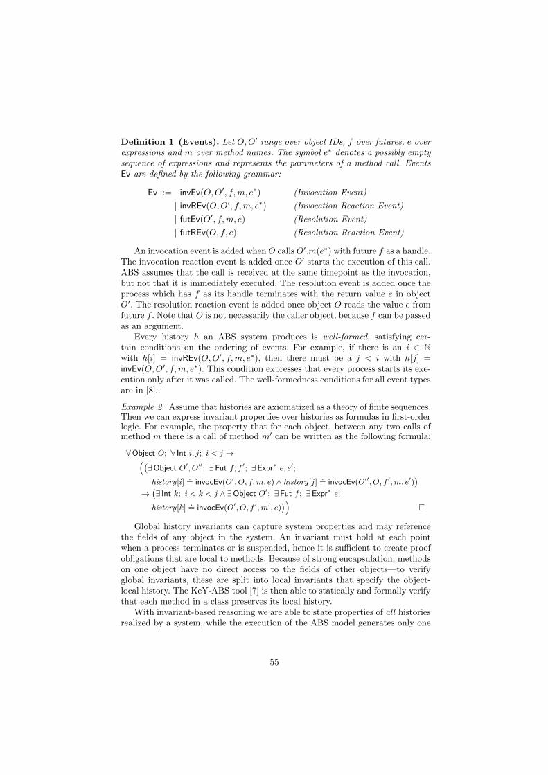
Definition 1 (Events). Let O, O0 range over object IDs, f over futures, e overexpressions and m over method names. The symbol e⇤ denotes a possibly emptysequence of expressions and represents the parameters of a method call. EventsEv are defined by the following grammar:
Ev ::= invEv(O, O0, f, m, e⇤) (Invocation Event)
| invREv(O, O0, f, m, e⇤) (Invocation Reaction Event)
| futEv(O0, f, m, e) (Resolution Event)
| futREv(O, f, e) (Resolution Reaction Event)
An invocation event is added when O calls O0.m(e⇤) with future f as a handle.The invocation reaction event is added once O0 starts the execution of this call.ABS assumes that the call is received at the same timepoint as the invocation,but not that it is immediately executed. The resolution event is added once theprocess which has f as its handle terminates with the return value e in objectO0. The resolution reaction event is added once object O reads the value e fromfuture f . Note that O is not necessarily the caller object, because f can be passedas an argument.
Every history h an ABS system produces is well-formed, satisfying cer-tain conditions on the ordering of events. For example, if there is an i 2 Nwith h[i] = invREv(O, O0, f, m, e⇤), then there must be a j < i with h[j] =invEv(O, O0, f, m, e⇤). This condition expresses that every process starts its exe-cution only after it was called. The well-formedness conditions for all event typesare in [8].
Example 2. Assume that histories are axiomatized as a theory of finite sequences.Then we can express invariant properties over histories as formulas in first-orderlogic. For example, the property that for each object, between any two calls ofmethod m there is a call of method m0 can be written as the following formula:
8Object O; 8 Int i, j; i < j !⇣�9Object O0, O00; 9Fut f, f 0; 9Expr⇤ e, e0;
history [i].= invocEv(O0, O, f, m, e) ^ history [j]
.= invocEv(O00, O, f 0, m, e0)
�
!�9 Int k; i < k < j ^ 9Object O0; 9Fut f ; 9Expr⇤ e;
history [k].= invocEv(O0, O, f 0, m0, e)
�⌘
Global history invariants can capture system properties and may referencethe fields of any object in the system. An invariant must hold at each pointwhen a process terminates or is suspended, hence it is su�cient to create proofobligations that are local to methods: Because of strong encapsulation, methodson one object have no direct access to the fields of other objects—to verifyglobal invariants, these are split into local invariants that specify the object-local history. The KeY-ABS tool [7] is then able to statically and formally verifythat each method in a class preserves its local history.
With invariant-based reasoning we are able to state properties of all historiesrealized by a system, while the execution of the ABS model generates only one
55
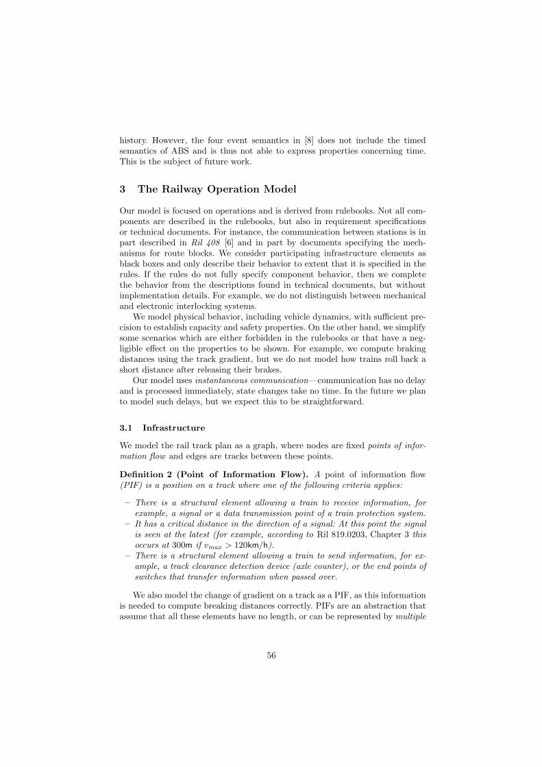
history. However, the four event semantics in [8] does not include the timedsemantics of ABS and is thus not able to express properties concerning time.This is the subject of future work.
3 The Railway Operation Model
Our model is focused on operations and is derived from rulebooks. Not all com-ponents are described in the rulebooks, but also in requirement specificationsor technical documents. For instance, the communication between stations is inpart described in Ril 408 [6] and in part by documents specifying the mech-anisms for route blocks. We consider participating infrastructure elements asblack boxes and only describe their behavior to extent that it is specified in therules. If the rules do not fully specify component behavior, then we completethe behavior from the descriptions found in technical documents, but withoutimplementation details. For example, we do not distinguish between mechanicaland electronic interlocking systems.
We model physical behavior, including vehicle dynamics, with su�cient pre-cision to establish capacity and safety properties. On the other hand, we simplifysome scenarios which are either forbidden in the rulebooks or that have a neg-ligible e↵ect on the properties to be shown. For example, we compute brakingdistances using the track gradient, but we do not model how trains roll back ashort distance after releasing their brakes.
Our model uses instantaneous communication—communication has no delayand is processed immediately, state changes take no time. In the future we planto model such delays, but we expect this to be straightforward.
3.1 Infrastructure
We model the rail track plan as a graph, where nodes are fixed points of infor-mation flow and edges are tracks between these points.
Definition 2 (Point of Information Flow). A point of information flow(PIF) is a position on a track where one of the following criteria applies:
– There is a structural element allowing a train to receive information, forexample, a signal or a data transmission point of a train protection system.
– It has a critical distance in the direction of a signal: At this point the signalis seen at the latest (for example, according to Ril 819.0203, Chapter 3 thisoccurs at 300m if vmax > 120km/h).
– There is a structural element allowing a train to send information, for ex-ample, a track clearance detection device (axle counter), or the end points ofswitches that transfer information when passed over.
We also model the change of gradient on a track as a PIF, as this informationis needed to compute breaking distances correctly. PIFs are an abstraction thatassume that all these elements have no length, or can be represented by multiple
56
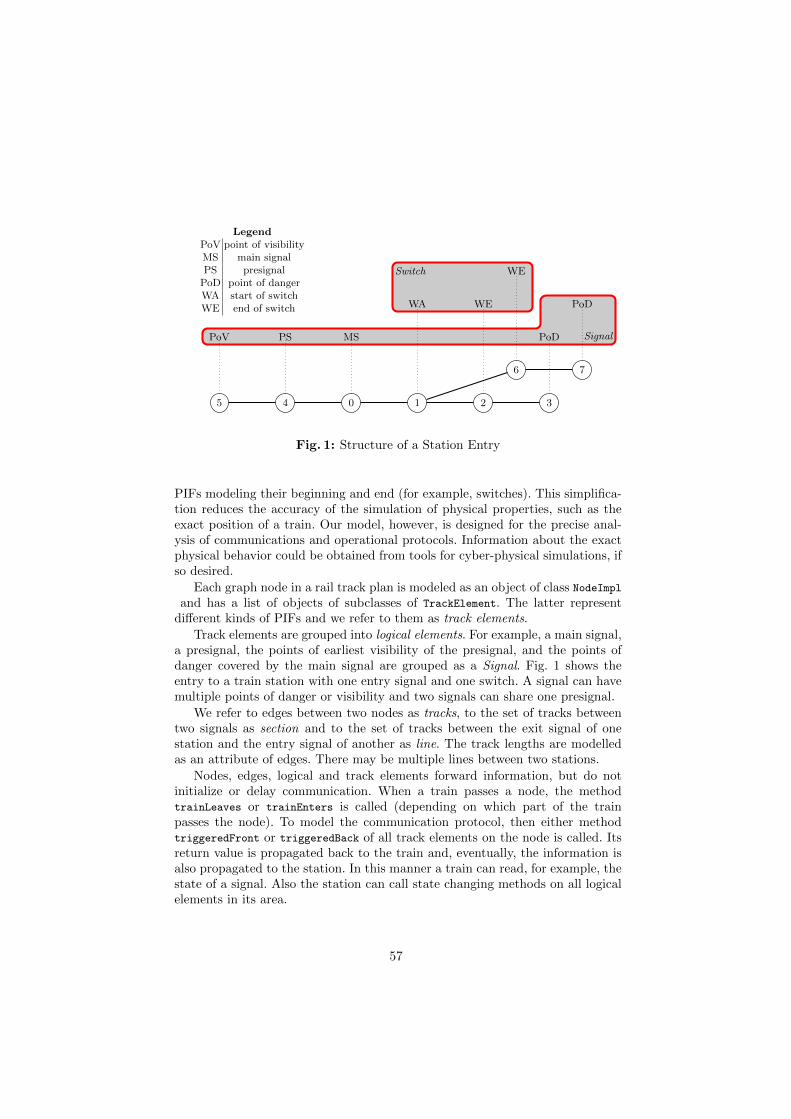
Signal
5 4 0 3
7
Switch
1 2
6
LegendPoV point of visibilityMS main signalPS presignal
PoD point of dangerWA start of switchWE end of switch
PoV PS MS PoD
PoDWA WE
WE
Fig. 1: Structure of a Station Entry
PIFs modeling their beginning and end (for example, switches). This simplifica-tion reduces the accuracy of the simulation of physical properties, such as theexact position of a train. Our model, however, is designed for the precise anal-ysis of communications and operational protocols. Information about the exactphysical behavior could be obtained from tools for cyber-physical simulations, ifso desired.
Each graph node in a rail track plan is modeled as an object of class NodeImpland has a list of objects of subclasses of TrackElement. The latter represent
di↵erent kinds of PIFs and we refer to them as track elements.
Track elements are grouped into logical elements. For example, a main signal,a presignal, the points of earliest visibility of the presignal, and the points ofdanger covered by the main signal are grouped as a Signal. Fig. 1 shows theentry to a train station with one entry signal and one switch. A signal can havemultiple points of danger or visibility and two signals can share one presignal.
We refer to edges between two nodes as tracks, to the set of tracks betweentwo signals as section and to the set of tracks between the exit signal of onestation and the entry signal of another as line. The track lengths are modelledas an attribute of edges. There may be multiple lines between two stations.
Nodes, edges, logical and track elements forward information, but do notinitialize or delay communication. When a train passes a node, the methodtrainLeaves or trainEnters is called (depending on which part of the trainpasses the node). To model the communication protocol, then either methodtriggeredFront or triggeredBack of all track elements on the node is called. Itsreturn value is propagated back to the train and, eventually, the information isalso propagated to the station. In this manner a train can read, for example, thestate of a signal. Also the station can call state changing methods on all logicalelements in its area.
57
A train only receives information about the current state of the track elementsat a node it passes. There is no direct communication between the train and thecontroller. Similarly, a train only initiates the communication that it passed anode, the station does not receive the identity of the train, only the informationthat it passed a point of danger. A station, however, knows which trains are inits area and a train knows which station is responsible for it. This is necessary sothat a station can issue emergency break orders, etc., and for a train to contact itsstation in case of a fault. The communication carried out during those situationsis carefully separated from regular communication in the model. Neither logicalnor track elements advance time.
3.2 Trains
Trains have two positions, front and end, each modeled as the distance on a trackrelative to the most recent node. For example, if the front of a train is on tracke, 5m behind a node n, then this position is described as (e, n, 5). A train hasa speed, an acceleration state (stable/braking/accelerating) and a length (thedistance between its front and its end) as well as attributes such as maximalacceleration and brake retardation that depend on the production series.
Edges maintain a pointer to the trains that pass them, so if a train occupiesmore than two edges the information that it occupies the edges in between thefirst and last is not lost.
Trains are modeled to drive on simulation events. At every PIF where thetrain is active, it computes its next event and the time until this event must beprocessed. There are three kinds of simulation events:
– The front of a train reaches the next node– The end of a train reaches the next node– A train stops accelerating/braking
When a train stops, it does not compute a new event. It can, however, receivea command, directly from the station or by observing a signal, set its state toaccelerating and continue driving.
Consider the simulation event when a train reaches a node n with its front.It receives information from all track elements at this node and changes its stateaccording to that information. Fig. 2 displays the method to process such anevent. Line 7 changes the state to an emergency brake when passing a “Stop” atthe main signal, unless Order 2 (pass the next “Stop” at a signal) was issued.
Not all events are computed by trains. A station can issue an order at anytime by calling method Train.command. In this case the train computes (i) itscurrent state, based on the current time and the most recent state, (ii) changesits state according to the issued order, (iii) computes, based on the state change,the next event. The process that waits for the old (now invalid order) cannot becanceled in ABS. Instead a counter of the number of orders the train receivedis increased. When the process of the defunct event is reactivated it checks thiscounter and immediately terminates if it has advanced.
58
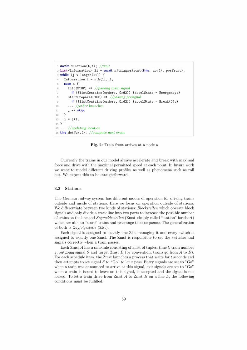
1 await duration(t,t); //wait2 List<Information> li = await n!triggerFront(this, now(), posFront);
3 while (j < length(li)) {
4 Information i = nth(li,j);
5 case i {
6 Info(STOP) => //passing main signal7 if (!listContains(orders, Ord2)) {accelState = Emergency;}
8 StartPrepare(STOP) => //passing presignal9 if (!listContains(orders, Ord2)) {accelState = Break(0);}
10 ... //other branches11 _ => skip;12 }
13 j = j+1;
14 }
15 ... //updating location16 this.detNext(); //compute next event
Fig. 2: Train front arrives at a node n
Currently the trains in our model always accelerate and break with maximalforce and drive with the maximal permitted speed at each point. In future workwe want to model di↵erent driving profiles as well as phenomena such as rollout. We expect this to be straightforward.
3.3 Stations
The German railway system has di↵erent modes of operation for driving trainsoutside and inside of stations. Here we focus on operation outside of stations.We di↵erentiate between two kinds of stations: Blockstellen which operate blocksignals and only divide a track line into two parts to increase the possible numberof trains on the line and Zugmeldestellen (Zmst, simply called “station” for short)which are able to “store” trains and rearrange their sequence. The generalizationof both is Zugfolgestelle (Zfst).
Each signal is assigned to exactly one Zfst managing it and every switch isassigned to exactly one Zmst. The Zmst is responsible to set the switches andsignals correctly when a train passes.
Each Zmst A has a schedule consisting of a list of tuples: time t, train numberz, outgoing signal S and target Zmst B (by convention, trains go from A to B).For each schedule item, the Zmst launches a process that waits for t seconds andthen attempts to set signal S to “Go” to let z pass. Entry signals are set to ”Go”when a train was announced to arrive at this signal, exit signals are set to ”Go”when a train is issued to leave on this signal, is accepted and the signal is notlocked. To let a train drive from Zmst A to Zmst B on a line L, the followingconditions must be fulfilled:
59
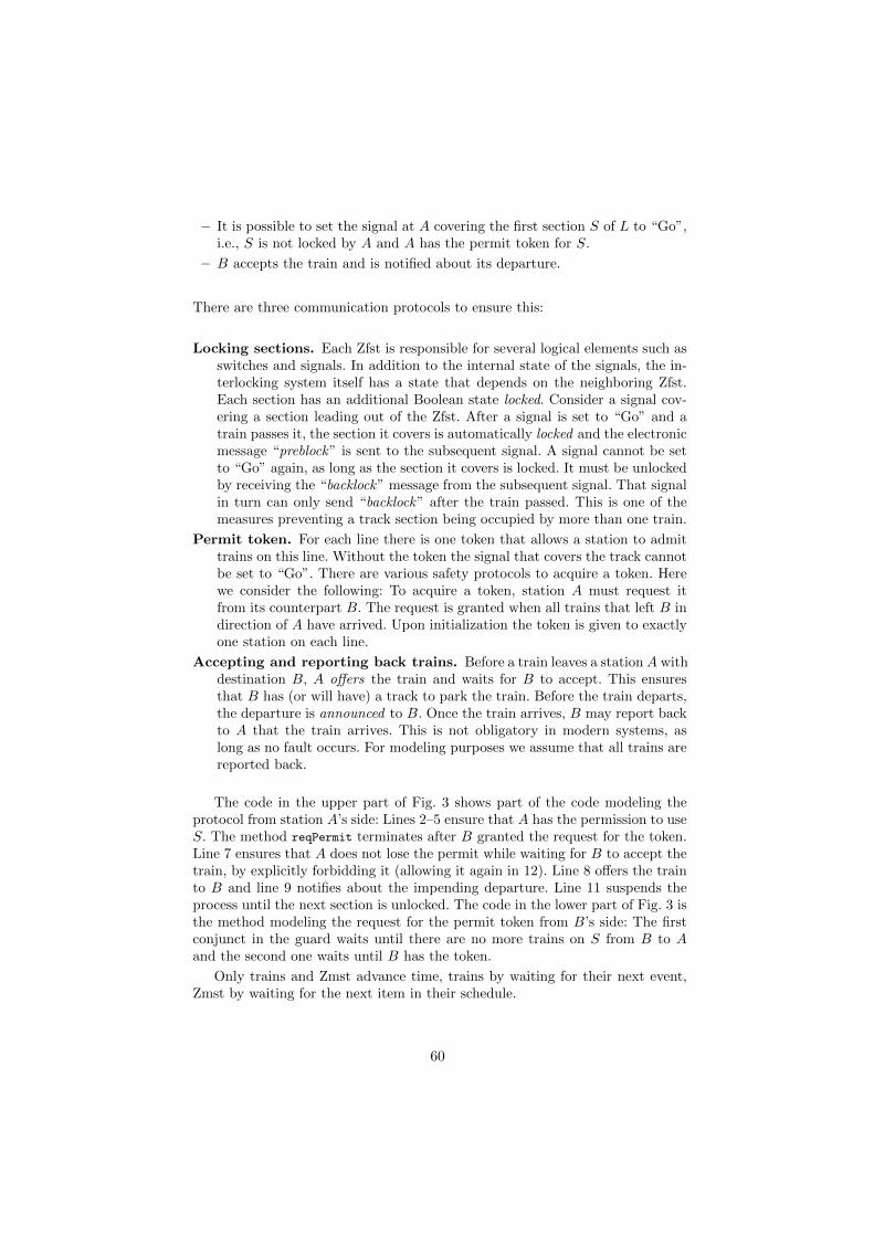
– It is possible to set the signal at A covering the first section S of L to “Go”,i.e., S is not locked by A and A has the permit token for S.
– B accepts the train and is notified about its departure.
There are three communication protocols to ensure this:
Locking sections. Each Zfst is responsible for several logical elements such asswitches and signals. In addition to the internal state of the signals, the in-terlocking system itself has a state that depends on the neighboring Zfst.Each section has an additional Boolean state locked. Consider a signal cov-ering a section leading out of the Zfst. After a signal is set to “Go” and atrain passes it, the section it covers is automatically locked and the electronicmessage “preblock” is sent to the subsequent signal. A signal cannot be setto “Go” again, as long as the section it covers is locked. It must be unlockedby receiving the “backlock” message from the subsequent signal. That signalin turn can only send “backlock” after the train passed. This is one of themeasures preventing a track section being occupied by more than one train.
Permit token. For each line there is one token that allows a station to admittrains on this line. Without the token the signal that covers the track cannotbe set to “Go”. There are various safety protocols to acquire a token. Herewe consider the following: To acquire a token, station A must request itfrom its counterpart B. The request is granted when all trains that left B indirection of A have arrived. Upon initialization the token is given to exactlyone station on each line.
Accepting and reporting back trains. Before a train leaves a station A withdestination B, A o↵ers the train and waits for B to accept. This ensuresthat B has (or will have) a track to park the train. Before the train departs,the departure is announced to B. Once the train arrives, B may report backto A that the train arrives. This is not obligatory in modern systems, aslong as no fault occurs. For modeling purposes we assume that all trains arereported back.
The code in the upper part of Fig. 3 shows part of the code modeling theprotocol from station A’s side: Lines 2–5 ensure that A has the permission to useS. The method reqPermit terminates after B granted the request for the token.Line 7 ensures that A does not lose the permit while waiting for B to accept thetrain, by explicitly forbidding it (allowing it again in 12). Line 8 o↵ers the trainto B and line 9 notifies about the impending departure. Line 11 suspends theprocess until the next section is unlocked. The code in the lower part of Fig. 3 isthe method modeling the request for the permit token from B’s side: The firstconjunct in the guard waits until there are no more trains on S from B to Aand the second one waits until B has the token.
Only trains and Zmst advance time, trains by waiting for their next event,Zmst by waiting for the next item in their schedule.
60
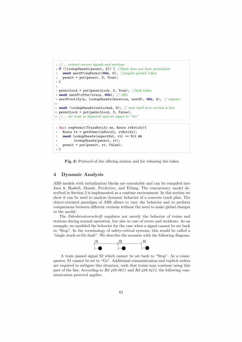
1 // ... extract correct signals and sections2 if (!lookupUnsafe(permit, S)) { //Zmst does not have permission3 await nextM!reqPermit(this, S); //acquire permit token4 permit = put(permit, S, True);
5 }
6
7 permitLock = put(permitLock, S, True); //lock token8 await nextM!offer(train, this); // o↵er9 nextM!notify(n, lookupUnsafe(duration, nextM), this, A); // register
10
11 await !lookupUnsafe(outLocked, S); // wait until next section is free12 permitLock = put(permitLock, S, False);
13 // ... set train as departed and set signal to ‘‘Go’’
1 Unit reqPermit(TrainNotify sw, Route rtNotify){
2 Route rt = getOther(inNotify, rtNotify);
3 await lookupUnsafe(expectOut, rt) == Nil &&
4 lookupUnsafe(permit, rt);
5 permit = put(permit, rt, False);
6 }
Fig. 3: Protocol of the o↵ering station and for releasing the token
4 Dynamic Analysis
ABS models with initialization blocks are executable and can be compiled intoJava 8, Haskell, Maude, ProActive, and Erlang. The concurrency model de-scribed in Section 2 is implemented as a runtime environment. In this section weshow it can be used to analyze dynamic behavior of a concrete track plan. Theobject-oriented paradigm of ABS allows to vary the behavior and to performcomparisons between di↵erent versions without the need to make global changesto the model.
The Fahrdienstvorschrift regulates not merely the behavior of trains andstations during normal operation, but also in case of errors and incidents. As anexample, we modeled the behavior for the case when a signal cannot be set backto “Stop”. In the terminology of safety-critical systems, this would be called a“single stuck-at-Go fault”. We describe the scenario with the following diagram:
A train passed signal S2 which cannot be set back to “Stop”. As a conse-quence, S1 cannot be set to “Go”. Additional communication and explicit ordersare required to mitigate this situation, such that trains may continue using thispart of the line. According to Ril 408.0611 and Ril 408.0411, the following com-munication protocol applies:
61
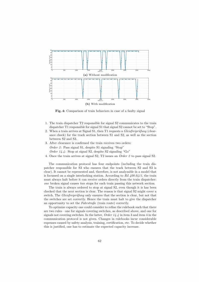
0
5
10
15
20
25
30
35
40
0 500 1000 1500 2000 2500 3000 3500 4000
velocityinm/s
timeins
(a) Without modification
0
5
10
15
20
25
30
35
40
0 500 1000 1500 2000 2500 3000 3500 4000
velocityinm/s
timeins
(b) With modification
Fig. 4: Comparison of train behaviors in case of a faulty signal
1. The train dispatcher T2 responsible for signal S2 communicates to the traindispatcher T1 responsible for signal S1 that signal S2 cannot be set to “Stop”.
2. When a train arrives at Signal S1, then T1 requests a Gleisfreiprufung (clear-ance check) for the track section between S1 and S2, as well as the sectionbetween S2 and S3.
3. After clearance is confirmed the train receives two orders:
Order 2 : Pass signal S1, despite S1 signaling “Stop”
Order 14.4 : Stop at signal S2, despite S2 signaling “Go”
4. Once the train arrives at signal S2, T2 issues an Order 2 to pass signal S2.
The communication protocol has four endpoints (including the train dis-patcher responsible for S3 who ensures that the track between S2 and S3 isclear). It cannot be represented and, therefore, is not analyzable in a model thatis focussed on a single interlocking station. According to Ril 408.0411, the trainmust always halt before it can receive orders directly from the train dispatcher:one broken signal causes two stops for each train passing this network section.
The train is always ordered to stop at signal S2, even though it is has beenchecked that the next section is clear. The reason is that signal S2 might cover aswitch. The Gleisfreiprufung only ensures that the section is clear, but not thatthe switches are set correctly. Hence the train must halt to give the dispatcheran opportunity to set the Fahrstraße (train route) correctly.
To optimize capacity one could consider to refine the rulebook such that thereare two rules—one for signals covering switches, as described above, and one forsignals not covering switches. In the latter, Order 14.4 in item 3 and item 4 in thecommunication protocol is not given. Changes in rulebooks incur considerableexpenses caused by safety analysis, training, certification, etc. To decide whetherthis is justified, one has to estimate the expected capacity increase.
62
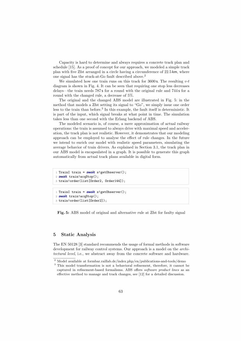
Capacity is hard to determine and always requires a concrete track plan andschedule [15]. As a proof of concept for our approach, we modeled a simple trackplan with five Zfst arranged in a circle having a circumference of 22.5 km, whereone signal has the stuck-at-Go fault described above.2
We simulated how one train runs on this track for 3600 s. The resulting v-tdiagram is shown in Fig. 4. It can be seen that requiring one stop less decreasesdelays—the train needs 787 s for a round with the original rule and 744 s for around with the changed rule, a decrease of 5%.
The original and the changed ABS model are illustrated in Fig. 5: in themethod that models a Zfst setting its signal to “Go”, we simply issue one orderless to the train than before.3 In this example, the fault itself is deterministic. Itis part of the input, which signal breaks at what point in time. The simulationtakes less than one second with the Erlang backend of ABS.
The modeled scenario is, of course, a mere approximation of actual railwayoperations: the train is assumed to always drive with maximal speed and acceler-ation, the track plan is not realistic. However, it demonstrates that our modelingapproach can be employed to analyse the e↵ect of rule changes. In the futurewe intend to enrich our model with realistic speed parameters, simulating theaverage behavior of train drivers. As explained in Section 3.1, the track plan inour ABS model is encapsulated in a graph. It is possible to generate this graphautomatically from actual track plans available in digital form.
1 TrainI train = await s!getObserver();
2 await train!acqStop();
3 train!order(list[Order2, Order144]);
1 TrainI train = await s!getObserver();
2 await train!acqStop();
3 train!order(list[Order2]);
Fig. 5: ABS model of original and alternative rule at Zfst for faulty signal
5 Static Analysis
The EN 50128 [3] standard recommends the usage of formal methods in softwaredevelopment for railway control systems. Our approach is a model on the archi-tectural level, i.e., we abstract away from the concrete software and hardware.
2 Model available at formbar.raillab.de/index.php/en/publications-and-tools/demo3 This model transformation is not a behavioral refinement, therefore, it cannot be
captured in refinement-based formalisms. ABS o↵ers software product lines as ane↵ective method to manage and track changes, see [12] for a detailed discussion.
63
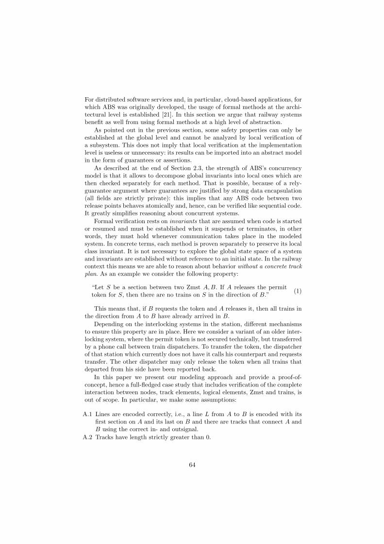
For distributed software services and, in particular, cloud-based applications, forwhich ABS was originally developed, the usage of formal methods at the archi-tectural level is established [21]. In this section we argue that railway systemsbenefit as well from using formal methods at a high level of abstraction.
As pointed out in the previous section, some safety properties can only beestablished at the global level and cannot be analyzed by local verification ofa subsystem. This does not imply that local verification at the implementationlevel is useless or unnecessary: its results can be imported into an abstract modelin the form of guarantees or assertions.
As described at the end of Section 2.3, the strength of ABS’s concurrencymodel is that it allows to decompose global invariants into local ones which arethen checked separately for each method. That is possible, because of a rely-guarantee argument where guarantees are justified by strong data encapsulation(all fields are strictly private): this implies that any ABS code between tworelease points behaves atomically and, hence, can be verified like sequential code.It greatly simplifies reasoning about concurrent systems.
Formal verification rests on invariants that are assumed when code is startedor resumed and must be established when it suspends or terminates, in otherwords, they must hold whenever communication takes place in the modeledsystem. In concrete terms, each method is proven separately to preserve its localclass invariant. It is not necessary to explore the global state space of a systemand invariants are established without reference to an initial state. In the railwaycontext this means we are able to reason about behavior without a concrete trackplan. As an example we consider the following property:
“Let S be a section between two Zmst A, B. If A releases the permittoken for S, then there are no trains on S in the direction of B.”
(1)
This means that, if B requests the token and A releases it, then all trains inthe direction from A to B have already arrived in B.
Depending on the interlocking systems in the station, di↵erent mechanismsto ensure this property are in place. Here we consider a variant of an older inter-locking system, where the permit token is not secured technically, but transferredby a phone call between train dispatchers. To transfer the token, the dispatcherof that station which currently does not have it calls his counterpart and requeststransfer. The other dispatcher may only release the token when all trains thatdeparted from his side have been reported back.
In this paper we present our modeling approach and provide a proof-of-concept, hence a full-fledged case study that includes verification of the completeinteraction between nodes, track elements, logical elements, Zmst and trains, isout of scope. In particular, we make some assumptions:
A.1 Lines are encoded correctly, i.e., a line L from A to B is encoded with itsfirst section on A and its last on B and there are tracks that connect A andB using the correct in- and outsignal.
A.2 Tracks have length strictly greater than 0.
64

Property (1) can be expressed as a history invariant which is formalized in first-order logic and can be verified with KeY-ABS [7]. In the following formula let
A, B be two Zmst and S, S two sections of a line L such hat S is the firstsection of L from A and S the first section of L from B. It expresses that whenA releases the permit token to B, every train that was announced from A to Bwas reported back by B to A.
8 Int i;�9Fut f ; h[i]
.= futEv(A, f, reqErlaubnis, (B, S))
�!
8Train T, Int j; j < i !⇣�9Fut F ; h[j]
.= invREv(A, B, f, anmelden, (T, t, A, S))
�! (2)
9 Int k, Fut f ; h[k].= invREv(B, A, f, rueckmeldung, (B, T, S)) ^ j < k < i
⌘
Theorem 1. Invariant (2) holds for method reqErlaubnis in Fig. 3 (and allother methods in its class), i.e., if it holds at the start of the method, then it isreestablished after termination.
This does not yet show that there are never two trains on one line in opposingdirections. To show that one must additionally establish that if a train entersa line, then it was o↵ered, accepted and announced and that when a train isreported back, then the train left the line. A proof sketch of Theorem 1 is in theAppendix. It has also been proven mechanically with the help of KeY-ABS.
6 Related Work
The work closest to ours is by James et al. [17], who presented a formalizationof ETCS level 2 in Real-Time Maude and analyze the communication betweentrains and one station. Like ours, their approach is set at the design level andencompasses all components needed for driving trains. However, it is restrictedto one specific rail yard, necessitated by the use of model checking instead ofdeductive invariant reasoning. A further di↵erence is that our work concentrateson ETCS level 1LS, which is the most relevant within the network of DeutscheBahn AG. Maude is an object-oriented language based on term rewriting andone of the backends supported by ABS. Therefore, potentially both modelingapproaches might be combined.
Individual rail yard components such as interlocking systems have been ana-lyzed by multiple approaches, for example, recently in SystemC [13], OCRA [19]and CSP||B [20]. An overview over approaches for interlocking systems, the mostfrequently analyzed component, can be found in the survey of Fantechi et al. [9]and a comparison of ABS with these approaches in [12].
There are two main approaches to combine micro- and macroscopic models:
– Relating several models of increasing abstraction level and using the ap-propriate one for a given use case. This is either done by generating moreabstract models on demand from a microscopic model or annotating therelation between a micro- and a macroscopic model. [4, 16]
65

– Mesoscopic modeling, which aims to be a middle ground in terms of abstrac-tion, tailored for a given use case. A recent application of this approach wasgenerating timetables by de Fabris et al. [5].
Our approach leans towards mesoscopic modeling, but achieves simplificationnot by summarizing multiple elements, but by abstracting from certain aspects.For example, we do model each magnet of the train protection system PZB, butassume these as having no length. Similarly, established mesoscopic models donot consider the communication layer, which is the main focus of our work.
7 Conclusion & Future Work
We presented an approach to modeling and analysis of railway systems basedon an object-oriented, concurrent, executable modeling language. The modelingformalism is able to unify aspects from micro- and macroscopic modeling andallows to analyze static (for example, safety) as well as dynamic (for example,delays) properties of a rail yard based on a single model. For static analysis weuse deductive invariant reasoning which allows to prove properties for any validtrack plan and initial configuration.
As the next step, we plan to calibrate and validate our model with real dataon a part of the actual railway network of Deutsche Bahn AG. This includesestablishing realistic driving profiles regaring acceleration and speed as well asto determine the precision of our approach in terms of train positions. On thesafety side, we plan to provide a formalization of all incident scenarios describedin the rulebooks [6] and to prove a suitable safety property for this model.Furthermore, we plan to use analysis tools developed for ABS software models,such as complexity and deadlock analysis [1, 10], to examine the properties ofthe rulebook and for carrying out a capacity analysis.
Acknowledgements. We thank Sebastian Schon for his insights into train operations
and the anonymous reviewers for helpful comments. This work is supported by FormbaR,
’Formalisierung von betrieblichen und anderen Regelwerken’, part of AG Signalling/DB
RailLab in the Innovation Alliance of Deutsche Bahn AG and TU Darmstadt.
References
1. E. Albert, P. Arenas, A. Flores-Montoya, S. Genaim, M. Gomez-Zamalloa,E. Martin-Martin, G. Puebla, and G. Roman-Dıez. SACO: static analyzer forconcurrent objects. In E. Abraham and K. Havelund, editors, Proc. TACAS, vol-ume 8413 of LNCS. Springer, 2014.
2. J. Bjørk, F. S. de Boer, E. B. Johnsen, R. Schlatte, and S. L. T. Tarifa. User-definedschedulers for real-time concurrent objects. ISSE, 9(1):29–43, 2013.
3. CENELEC. DIN EN 50128:2011, Railway applications – Communication, Sig-nalling and Processing Signals.
4. Y. Cui and U. Martin. Multi-scale simulation in railway planning and operation.Promet Tra�c&Transportation, 23(6):511–517, 2011.
66
5. S. de Fabris, G. Longo, G. Medeossi, and R. Pesenti. Automatic generation ofrailway timetables based on a mesoscopic infrastructure model. Journal of RailTransport Planning & Management, 4(12):2–13, 2014.
6. Deutsche Bahn Netz AG, Frankfurt, Germany. Fahrdienstvorschrift Richtlinie 408.August 2016: fahrweg.dbnetze.com/fahrweg-de/nutzungsbedingungen/regelwerke/betriebl technisch/eiu interne regeln ril 408.html.
7. C. C. Din, R. Bubel, and R. Hahnle. KeY-ABS: A deductive verification tool forthe concurrent modelling language ABS. In A. P. Felty and A. Middeldorp, editors,CADE, volume 9195 of LNCS, pages 517–526. Springer, 2015.
8. C. C. Din and O. Owe. Compositional reasoning about active objects with sharedfutures. Formal Aspects of Computing, 27(3):551–572, 2015.
9. A. Fantechi, F. Flammini, and S. Gnesi. Formal methods for railway control sys-tems. STTT, 16(6):643–646, 2014.
10. E. Giachino, C. Laneve, and M. Lienhardt. A framework for deadlock detection incore abs. Software & Systems Modeling, 15(4):1013–1048, 2016.
11. R. Hahnle. The abstract behavioral specification language: A tutorial introduction.In E. Giachino, R. Hahnle, F. S. de Boer, and M. M. Bonsangue, editors, Proc.Formal Methods for Component-Based Systems FMCO, pages 1–37, 2012.
12. R. Hahnle and R. Muschevici. Towards incremental validation of railway systems.In T. Margaria and B. Ste↵en, editors, Leveraging Applications of Formal Methods,Verification and Validation, 7th International Symposium (ISoLA), Part II, Corfu,Greece, volume 9953 of LNCS, pages 433–446. Springer, Oct. 2016.
13. A. E. Haxthausen, J. Peleska, and S. Kinder. A formal approach for the construc-tion and verification of railway control systems. Formal Aspects of Computing,23(2):191–219, 2011.
14. C. Hewitt, P. Bishop, and R. Steiger. A universal modular ACTOR formalism forartificial intelligence. In N. J. Nilsson, editor, Proceedings of the 3rd InternationalJoint Conference on Artificial Intelligence. Standford, CA, USA, August 20-23,1973, pages 235–245. William Kaufmann, 1973.
15. International Union of Railways (UIC). Capacity (UIC code 406), 2004.16. International Union of Railways (UIC). IRS 30100 - RailTopoModel - Railway
Infrastructuretopological Model, 2016.17. P. James, A. Lawrence, M. Roggenbach, and M. Seisenberger. Towards safety anal-
ysis of ERTMS/ETCS level 2 in Real-Time Maude. In C. Artho and P. Olveczky,editors, Formal Techniques for Safety-Critical Systems FTSCS, Revised SelectedPapers, volume 596 of CCIS, pages 103–120. Springer, 2015.
18. E. B. Johnsen, R. Hahnle, J. Schafer, R. Schlatte, and M. Ste↵en. ABS: A corelanguage for abstract behavioral specification. In B. K. Aichernig, F. S. de Boer,and M. M. Bonsangue, editors, Proc. Formal Methods for Components and ObjectsFMCO, volume 6957 of LNCS. Springer, 2010.
19. C. Limbree, Q. Cappart, C. Pecheur, and S. Tonetta. Verification of railway in-terlocking, compositional approach with OCRA. In T. Lecomte, R. Pinger, andA. Romanovsky, editors, Reliability, Safety, and Security of Railway Systems. Mod-elling, Analysis, Verification, and Certification, RSSRail, volume 9707 of LNCS,pages 134–149. Springer, 2016.
20. F. Møller, H. N. Nguyen, M. Roggenbach, S. Schneider, and H. Treharne. Definingand model checking abstractions of complex railway models using CSP||B. InHardware and Software: Verification and Testing HVC, Revised Selected Papers,volume 7857 of LNCS, pages 193–208. Springer, 2012.
21. C. Newcombe, T. Rath, F. Zhang, B. Munteanu, M. Brooker, and M. Deardeu↵.How Amazon web services uses formal methods. CACM, 58(4):66–73, 2015.
67
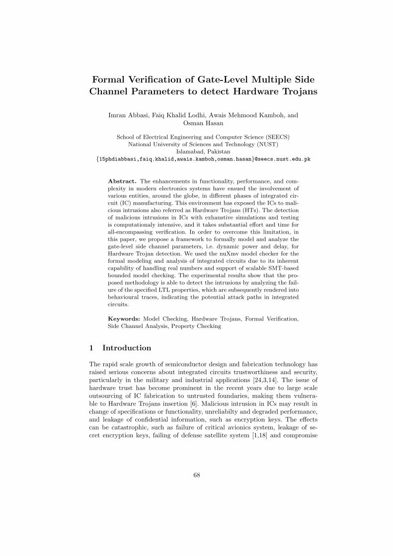
Formal Verification of Gate-Level Multiple SideChannel Parameters to detect Hardware Trojans
Imran Abbasi, Faiq Khalid Lodhi, Awais Mehmood Kamboh, andOsman Hasan
School of Electrical Engineering and Computer Science (SEECS)National University of Sciences and Technology (NUST)
Islamabad, Pakistan{15phdiabbasi,faiq.khalid,awais.kamboh,osman.hasan}@seecs.nust.edu.pk
Abstract. The enhancements in functionality, performance, and com-plexity in modern electronics systems have ensued the involvement ofvarious entities, around the globe, in di↵erent phases of integrated cir-cuit (IC) manufacturing. This environment has exposed the ICs to mali-cious intrusions also referred as Hardware Trojans (HTs). The detectionof malicious intrusions in ICs with exhaustive simulations and testingis computationaly intensive, and it takes substantial e↵ort and time forall-encompassing verification. In order to overcome this limitation, inthis paper, we propose a framework to formally model and analyze thegate-level side channel parameters, i.e. dynamic power and delay, forHardware Trojan detection. We used the nuXmv model checker for theformal modeling and analysis of integrated circuits due to its inherentcapability of handling real numbers and support of scalable SMT-basedbounded model checking. The experimental results show that the pro-posed methodology is able to detect the intrusions by analyzing the fail-ure of the specified LTL properties, which are subsequently rendered intobehavioural traces, indicating the potential attack paths in integratedcircuits.
Keywords: Model Checking, Hardware Trojans, Formal Verification,Side Channel Analysis, Property Checking
1 Introduction
The rapid scale growth of semiconductor design and fabrication technology hasraised serious concerns about integrated circuits trustworthiness and security,particularly in the military and industrial applications [24,3,14]. The issue ofhardware trust has become prominent in the recent years due to large scaleoutsourcing of IC fabrication to untrusted foundaries, making them vulnera-ble to Hardware Trojans insertion [6]. Malicious intrusion in ICs may result inchange of specifications or functionality, unreliabilty and degraded performance,and leakage of confidential information, such as encryption keys. The e↵ectscan be catastrophic, such as failure of critical avionics system, leakage of se-cret encryption keys, failing of defense satellite system [1,18] and compromise
68
2 I. Abbasi, F.K. Lodhi, A. Kamboh, O. Hasan
of heterogeneous network of Internet of Things (IoTs) [20]. Hardware Trojansare generally of two types: i) functional Trojans change the system functionalityby addition or deletion functional units in a circuit with malicious purpose andii) parametric Trojans reduce reliability of the IC to increase the likelihood ofsystem failure by modifying physical parameters, such as modifying the powerconsumption resulting in faster aging than expected.
Hardware Trojan detection schemes are broadly classified into logic basedtesting, side channel analysis and reverse engineering [5]. Logic based testingtechniques uses generation of random test vectors and implementation of dif-ferent methods to trigger the Trojan circuits and observe their e↵ects at theoutput [9]. Side channel analysis is based on measuring the variations in ob-servable physical parameters, such as delay, power, electromagnetic (EM) signalanalysis and current sensing in order to detect any alteration with the structuralcharacterization of the integrated circuit design [12]. Side channel analysis tech-niques are more commonly used because of their higher performance, relativelylower costs and nondestructive testing capabilities. Agarwal et. al. proposed apower analysis based technique by applying random patterns at inputs of ICsunder test and comparing their measurements with the power signature of agolden model [2]. The golden IC model is obtained from reverse engineering oflimited number of ICs. Similarly, Wang et. al. proposed to generate average andcovariance based power traces [25] employing the singular value decomposition(SVD) algorithm and eigenvector projection analysis, respectively, to detect themalicious intrusions. The focus of delay based detection techniques [15,22] is onthe delay measurements of individual paths of the circuit due to activation ofHardware Trojans and their comparison with of delay fingerprints from goldenICs. These above-mentioned delay and power signature analysis techniques arebased on extensive simulations or by testing on real hardware systems, which re-quires immense time, cost and resources. Moreover, the measurements acquiredthrough sensors cannot encompass all the possible input conditions for largerICs and result in an extensive amount of data, which is di�cult to handle withconventional automation techniques.
Formal verification [13] can overcome the above stated limitations of simu-lation based techniques for Hardware Trojan detection by virtue of its inherentsoundness and completeness. The formal verification based methods, such asSAT solving and Model Checking, have been used with the soft intellectualproperty(IP) of the IC to detect Hardware Trojans, provided that user has ac-cess to a hardware description language code or neltlist of the IC. In the recentpast, researchers have presented di↵erent frameworks for the formalization andverification of IP core security properties. Xuehui et. al. proposed an approachthat applies multistage assertion based verification, equivalence and code cov-erage analysis, redundant circuit removal for isolation of suspicious signals, andsequential automatic test pattern generations (ATPG) [29]. Rathmair et. al. havepresented a property checking based method which verifies functional propertiesdeduced from system specification using a model checker. The counterexampleis subsequently analyzed to detect potential attack paths [23]. Ngo et. al. have
69
Formal Verification of Gate Level Multiple Side Channel Parameters 3
presented a methodology to use assertions derived from temporal logic and con-verting them into a synthesizable checker. This method involves identificationand verification of critical behavioral invariants using assertion based propertyspecification language (PSL). The verified behavioral invariants are used to de-sign the hardware property checker (HPC) and subsequently integrated in ICsto verify the properties. However, to the best of our knowledge, so far no work isbeing reported, which considers the formal verification of performance proper-ties to detect intentional malicious enhancement of hardware design. Moreover,the above-mentioned assertion based property checking methods are vulnerableto Trojan insertions at netlist and layout levels, and will only be able to detectfunctional Trojans.
In this paper, we present a generic framework based on the behavioral modelof the IC to detect malicious hardware intrusions. We assume the attack modelB [28], in which we have a netlist available in the form of trusted design, butthe foundry is considered untrusted to which the design is outsourced for manu-facturing. The attacker in the foundry can insert Hardware Trojans in the formof addition, deletion or modification of gates. The main idea is to translate thecircuit netlist to a state transition system based model and verify it against theidentified set of functional and behavioral properties that can be a↵ected by anymalicious modification in the IC. The model is then intruded with the expectedmalicious behaviour, and counterexamples are analyzed for deducing potentialattack paths. On the basis of the information extracted from the detailed analy-sis of counterexamples, the designers can merge protection in the original designby embedding runtime hardware monitors. The proposed LTL properties arebased on system functional and physical behavior. We propose to use the sym-bolic model checker nuXmv [8] for analysis by virtue of its ability to handle realnumbers and implicit dealing of state counters.
The rest of this paper is organized as follows: Section 2 provides an overviewof the nuXmv model checker and performance parameters used in our gate mod-els. In Section 3, we explained the proposed methodology for hardware intrusiondetection followed by our gate modeling in the nuXmv model checker in Section4. In Section 5, we have given a case study for our proposed methodology. Sec-tion 6 presents the results followed by a comparison with some of the existingschemes in section 7. Finally, the paper concludes in Section 8.
2 Preliminaries
In this section, we give a brief introduction to the nuXmv model checker and theperformance parameters that we have used for the proposed Hardware Trojandetection process. The intent is to facilitate the understanding of the rest of thepaper for both hardware security and formal methods communities.
2.1 nuXmv Model Checker
The nuXmv symbolic model checker [8] is a recently developed formal verificationtool that extends the capabilities of NuSMV model checker [10], by supporting
70
4 I. Abbasi, F.K. Lodhi, A. Kamboh, O. Hasan
analysis of infinite state domains. It complements NuSMV’s verification tech-niques by sharing basic functionalities, such as symbol table, boolean encodingof scalar variables, flattening of design, and representation of finite state ma-chines at di↵erent levels of abstraction. Moreover, it inherits all the basic modelchecking algorithms from NuSMV for finite domains using BDDs and SAT. Forinfinite state transition models, it introduces new data types of unbounded In-tegers and Reals and it provides the support of Satisfiability Modulo Theories(SMT), using MathSAT [17], for the analysis of such kinds of designs. The systemthat is required to be modeled is translated into SMV language, which supportsthe modular programming approach. The entire system can be distributed intoseveral modules that interact with one another in the MAIN module. The proper-ties to be checked can be expressed in nuXmv using the Linear Temporal Logic(LTL) and Computation Tree Logic (CTL). The specifications are expressed innuXmv with the help of logical operations like, OR (|), AND (&), Exclusive OR(xor), Exclusive NOR (xnor), equality (<->), implication (->), and temporaloperators, like next (X), Globally (G), Finally (F) and until (U). Similarly, theCTL specifications can be written by combining logical operations with quan-tified temporal operators, like forall finally (AF), exists globally (EG) and existsnext state (EX). It is also possible to analyze quantitative characteristics of thestate transition system by specifying real-time specifications. Whenever a spec-ified property is determined to be false, a counterexample is constructed andsubsequently printed by nuXmv in the form of an error trace of the state spacethat falsifies the property. We have chosen the nuXmv model checker because itcan e↵ectively model continuous values of power consumption and path delaysof any given IC.
2.2 Performance Parameters
Gate level characterization has e↵ectively formed the basis of side channel Hard-ware Trojan detection schemes, which are based on characterizing each gate interms of its physical and performance parameters. We adopted dynamic powerconsumption and delay as the side channel performance parameters for mali-cious intrusion detection in any given circuit. Equation 1 represents the gatelevel switching power model [27] that is dependent upon the activity factor ↵,output capacitance CL, supply voltage Vdd, which has quadratic e↵ect on dy-namic power, and operating frequency f . The activity factor is the switchingprobability that a node of a circuit transitions from 0 to 1, because that is theonly time when dynamic power is consumed by the circuit in the CMOS tech-nology. The total output capacitance is the sum of parasitic capacitance of theindividual gate and load capacitances at the output node.
Pswitching = ↵CtotalVdd2f (1)
We have estimated gate level delays based on individual transitions at thegate inputs using the Elmore delay model [27], which computes the delay byrepresenting each circuit in the form of RC tree. The voltage source is the root
71
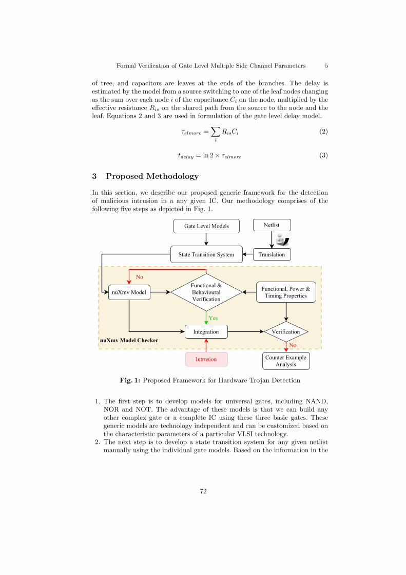
Formal Verification of Gate Level Multiple Side Channel Parameters 5
of tree, and capacitors are leaves at the ends of the branches. The delay isestimated by the model from a source switching to one of the leaf nodes changingas the sum over each node i of the capacitance Ci on the node, multiplied by thee↵ective resistance Ris on the shared path from the source to the node and theleaf. Equations 2 and 3 are used in formulation of the gate level delay model.
⌧elmore =X
i
RisCi (2)
tdelay = ln 2 ⇥ ⌧elmore (3)
3 Proposed Methodology
In this section, we describe our proposed generic framework for the detectionof malicious intrusion in a any given IC. Our methodology comprises of thefollowing five steps as depicted in Fig. 1.
Fig. 1: Proposed Framework for Hardware Trojan Detection
1. The first step is to develop models for universal gates, including NAND,NOR and NOT. The advantage of these models is that we can build anyother complex gate or a complete IC using these three basic gates. Thesegeneric models are technology independent and can be customized based onthe characteristic parameters of a particular VLSI technology.
2. The next step is to develop a state transition system for any given netlistmanually using the individual gate models. Based on the information in the
72
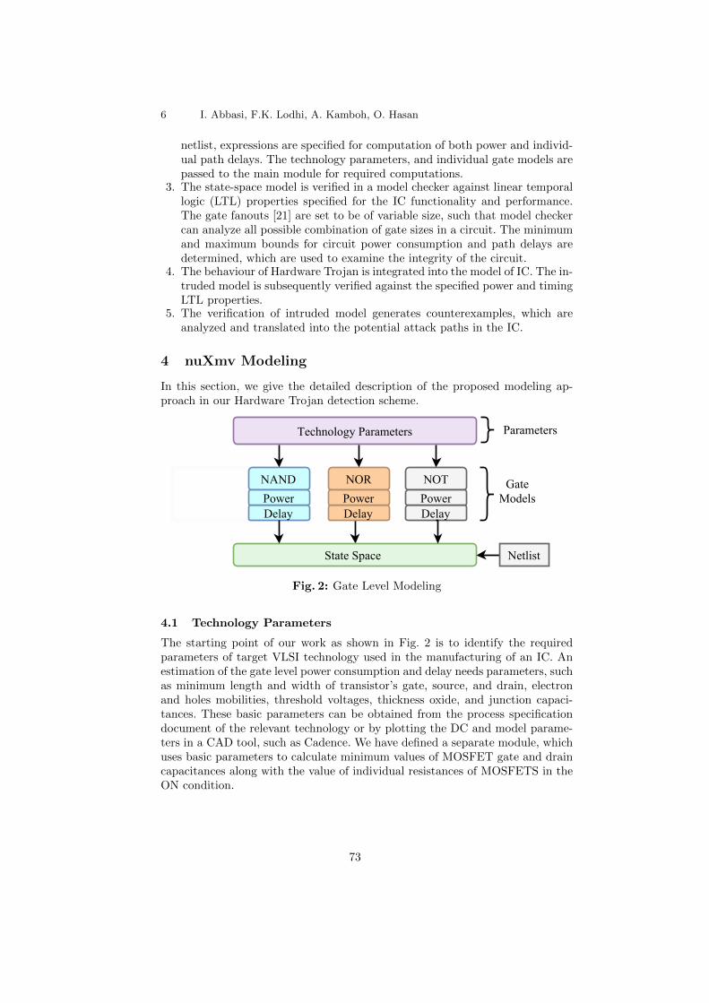
6 I. Abbasi, F.K. Lodhi, A. Kamboh, O. Hasan
netlist, expressions are specified for computation of both power and individ-ual path delays. The technology parameters, and individual gate models arepassed to the main module for required computations.
3. The state-space model is verified in a model checker against linear temporallogic (LTL) properties specified for the IC functionality and performance.The gate fanouts [21] are set to be of variable size, such that model checkercan analyze all possible combination of gate sizes in a circuit. The minimumand maximum bounds for circuit power consumption and path delays aredetermined, which are used to examine the integrity of the circuit.
4. The behaviour of Hardware Trojan is integrated into the model of IC. The in-truded model is subsequently verified against the specified power and timingLTL properties.
5. The verification of intruded model generates counterexamples, which areanalyzed and translated into the potential attack paths in the IC.
4 nuXmv Modeling
In this section, we give the detailed description of the proposed modeling ap-proach in our Hardware Trojan detection scheme.
Fig. 2: Gate Level Modeling
4.1 Technology Parameters
The starting point of our work as shown in Fig. 2 is to identify the requiredparameters of target VLSI technology used in the manufacturing of an IC. Anestimation of the gate level power consumption and delay needs parameters, suchas minimum length and width of transistor’s gate, source, and drain, electronand holes mobilities, threshold voltages, thickness oxide, and junction capaci-tances. These basic parameters can be obtained from the process specificationdocument of the relevant technology or by plotting the DC and model parame-ters in a CAD tool, such as Cadence. We have defined a separate module, whichuses basic parameters to calculate minimum values of MOSFET gate and draincapacitances along with the value of individual resistances of MOSFETS in theON condition.
73
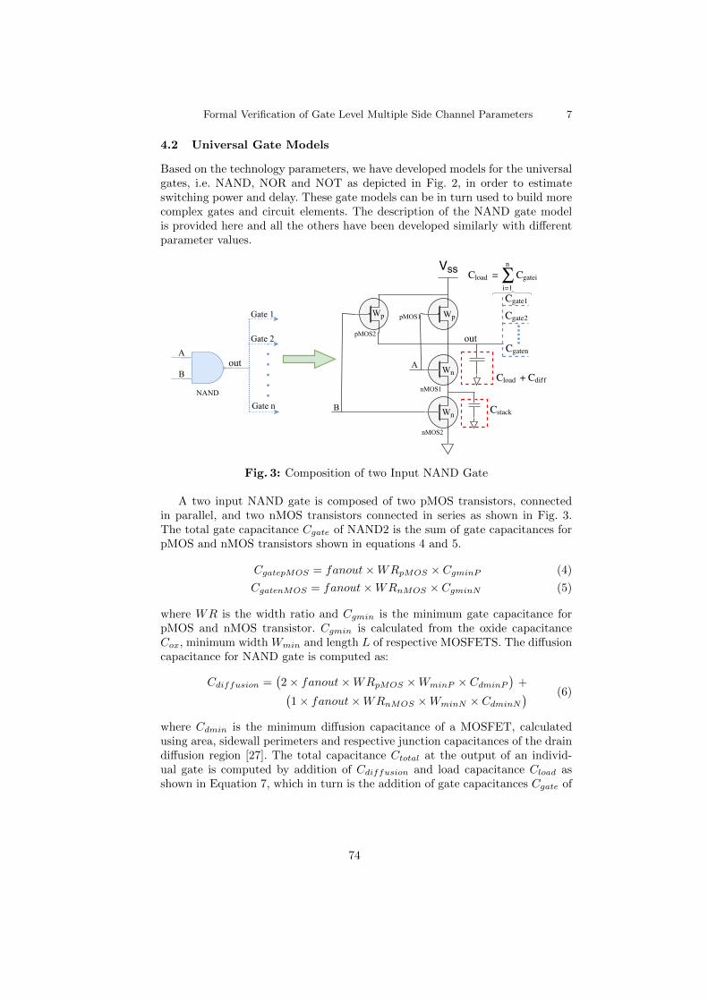
Formal Verification of Gate Level Multiple Side Channel Parameters 7
4.2 Universal Gate Models
Based on the technology parameters, we have developed models for the universalgates, i.e. NAND, NOR and NOT as depicted in Fig. 2, in order to estimateswitching power and delay. These gate models can be in turn used to build morecomplex gates and circuit elements. The description of the NAND gate modelis provided here and all the others have been developed similarly with di↵erentparameter values.
Fig. 3: Composition of two Input NAND Gate
A two input NAND gate is composed of two pMOS transistors, connectedin parallel, and two nMOS transistors connected in series as shown in Fig. 3.The total gate capacitance Cgate of NAND2 is the sum of gate capacitances forpMOS and nMOS transistors shown in equations 4 and 5.
CgatepMOS = fanout ⇥ WRpMOS ⇥ CgminP (4)
CgatenMOS = fanout ⇥ WRnMOS ⇥ CgminN (5)
where WR is the width ratio and Cgmin is the minimum gate capacitance forpMOS and nMOS transistor. Cgmin is calculated from the oxide capacitanceCox, minimum width Wmin and length L of respective MOSFETS. The di↵usioncapacitance for NAND gate is computed as:
Cdiffusion =�2 ⇥ fanout ⇥ WRpMOS ⇥ WminP ⇥ CdminP
�+
�1 ⇥ fanout ⇥ WRnMOS ⇥ WminN ⇥ CdminN
� (6)
where Cdmin is the minimum di↵usion capacitance of a MOSFET, calculatedusing area, sidewall perimeters and respective junction capacitances of the draindi↵usion region [27]. The total capacitance Ctotal at the output of an individ-ual gate is computed by addition of Cdiffusion and load capacitance Cload asshown in Equation 7, which in turn is the addition of gate capacitances Cgate of
74
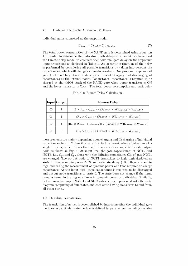
8 I. Abbasi, F.K. Lodhi, A. Kamboh, O. Hasan
individual gates connected at the output node.
Ctotal = Cload + Cdiffusion (7)
The total power consumption of the NAND gate is determined using Equation1. In order to determine the individual path delays in a circuit, we have usedthe Elmore delay model to calculate the individual gate delay on the respectiveinput transitions as depicted in Table 1. An accurate estimation of the delayis performed by considering all possible transitions by taking into account thecapacitances, which will change or remain constant. Our proposed approach ofgate level modeling also considers the e↵ects of charging and discharging ofcapacitances at the internal nodes. For instance, capacitance is required to becharged at the nMOS stack of the NAND gate when upper transistor is ONand the lower transistor is OFF. The total power consumption and path delay
Table 1: Elmore Delay Calculation
Input Output Elmore Delay
00 1 (2 ⇥ Rp ⇥ Ctotal) / (Fanout ⇥ WRpMOS ⇥ WminP )
01 1 (Rn ⇥ Ctotal) / (Fanout ⇥ WRnMOS ⇥ WminN )
10 1 (Rn ⇥ (Ctotal + CstackN )) / (Fanout ⇥ WRnMOS ⇥ WminN )
11 0 (Rn ⇥ Ctotal) / (Fanout ⇥ WRnMOS ⇥ WminN )
measurements are mainly dependent upon charging and discharging of individualcapacitances in an IC. We illustrate this fact by considering a behaviour of asingle inverter, which drives the load of two inverters connected at its outputnode as shown in Fig. 4. At input low, the gate capacitances of NOT2 andNOT3, i.e., Cg2 and Cg3 along with the di↵usion capacitance Cd1 of gate NOT1are charged. The output node of NOT1 transitions to logic high depicted asstate 1. The compute power(CP ) and estimate delay (ED) flags are set tohigh, indicating the measurement of dynamic power and time required to chargecapacitance. At the input high, same capacitance is required to be dischargedand output node transitions to state 0. The state does not change if the inputremains same, indicating no change in dynamic power or path delay. Similarly,behaviour of two input NAND and NOR gates can be represented with the statediagram comprising of four states, and each state having transitions to and from,all other states.
4.3 Netlist Translation
The translation of netlist is accomplished by interconnecting the individual gatemodules. A particular gate module is defined by parameters, including variable
75
Formal Verification of Gate Level Multiple Side Channel Parameters 9
Fig. 4: The State-Space Model of an Inverter
inputs, transition probabilities, gate capacitances at output, fanout and rele-vant technology parameters. The transition probabilities along with outputs arepassed to all gates connected at the output node of an individual gate. Othergates are constructed using the three basic gates, for instance, the AND gate isconstructed using a NAND module followed by a NOT gate. Similarly, netlistof any integrated circuit can be manually translated using basic models of thethree gates. The individual fanouts are swept across all the values in order toidentify maximum and minimum bounds of switching power and individual pathdelays.
4.4 Property Specification
The verification of the IC model is carried out by validating the following prop-erties using the bounded model checking (BMC) support for real numbers. Theperformance properties are validated using the nuXmv model checker to ascer-tain that the given IC remains between the specified boundaries defined fordynamic power and delay parameters. The undesired behaviour of the circuitdue to any malicious alteration of circuit can be identified from the generatedcounterexample. The maximum and minimum bounds for power consumptionare identified to validate the power property. The LTL specifications to validatethe switching power is defined by adding the power consumed by individual gatesin the circuit.
G(pwr max >= gate1.pwr + gate2.pwr + ... + gaten.pwr >= pwr min) (I)
The attacker can intrude the IC by altering and modifying any of the individualpath from input to output. Therefore, the characteristic delay of each individualpath in an IC from input to output is required to be validated using the delaybased properties. Suppose an IC has p number of paths from input to output,
76
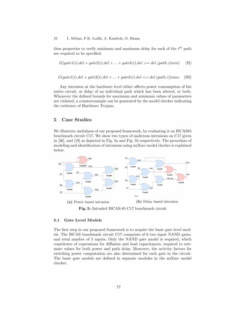
10 I. Abbasi, F.K. Lodhi, A. Kamboh, O. Hasan
then properties to verify minimum and maximum delay for each of the ith pathare required to be specified.
G(gate1(i).del + gate2(i).del + ... + gatek(i).del >= del (path i)min) (II)
G(gate1(i).del + gate2(i).del + ... + gatek(i).del <= del (path i))max (III)
Any intrusion at the hardware level either a↵ects power consumption of theentire circuit, or delay of an individual path which has been altered, or both.Whenever the defined bounds for maximum and minimum values of parametersare violated, a counterexample can be generated by the model checker indicatingthe existence of Hardware Trojans.
5 Case Studies
We illustrate usefulness of our proposed framework, by evaluating it on ISCAS85benchmark circuit C17. We show two types of malicious intrusions on C17 givenin [26], and [19] as depicted in Fig. 5a and Fig. 5b respectively. The procedure ofmodeling and identification of intrusions using nuXmv model checker is explainedbelow.
(a) Power based intrusion (b) Delay based intrusion
Fig. 5: Intruded ISCAS-85 C17 benchmark circuit
5.1 Gate Level Models
The first step in our proposed framework is to acquire the basic gate level mod-els. The ISCAS benchmark circuit C17 comprises of 6 two input NAND gates,and total number of 5 inputs. Only the NAND gate model is required, whichconstitutes of expressions for di↵usion and load capacitances, required to esti-mate values for both power and path delay. Moreover, the activity factors forswitching power computation are also determined for each gate in the circuit.The basic gate models are defined in separate modules in the nuXmv modelchecker.
77

Formal Verification of Gate Level Multiple Side Channel Parameters 11
5.2 State Space Modeling
The netlist gives the description of connectivity for C17 benchmark circuit, whichis translated into the state space. For example, consider the NAND3 gate in Fig.5a which has inputs N2, and NAND2.out (output of NAND2). The gate alongwith relevant parameters is described as:
NAND3:nand(N2, NAND2.out, 0.5, 0.5, NAND2.P0, NAND2.P1, Fanout3, par.Freq,
par.Cgmin p, par.Cgmin n, par.Vdd, par.Wmin, par.Cdmin p, par.Cdmin n,
par.Csmin p, par.Csmin n,par.Rp, par.Rn, NAND5.Cgate, NAND6.Cgate,0, 0);
Using the given input signal probabilities of the circuit, we compute the proba-bilities and activity factor for its each node. For example, input N2 has an inputprobability of 0.5 for 0 and 1, P0 and P1 are the probabilities of the second inputbeing 0 or 1, which can be used to calculate the activity factor at the pertinentnode of circuit. This follows by the parameters like, operating frequency, inputvoltage Vdd, values of gate and di↵usion capacitances, along with the values ofON resistances Rp and Rn for pMOS and nMOS transistors, respectively. Thelast part of the expression indicates the total load at the output node N16, whichis the sum of gate capacitance of NAND5 and NAND6. Typically, gates havethe maximum fanout of 4 and minimum fanout of 1[21]. Similarly, all six NANDgates of C17 circuit are described in the main module of nuXmv to generate theformal model of the given circuit.
5.3 Model Verification
After the state space of the C17 benchmark circuit is defined, the next step is tocheck the functionality the circuit. There are a total number of 25 = 32 possibleinput vector for C17 circuit. We verified the functionality of circuit by usingcertain number of input vectors. The next step is to identify the maximum andminimum bounds for switching power and delay. Our model accuracy requiresthe values to remain in between these bounds. The power for C17 circuit ismaximum when all 6 NAND gates have a maximum fanout equal to 4. Similarly,the minimum bound is determined by computing the power with the minimumfanout of 1. For all sizes of the gates of the C17 benchmark, the power forC17 is required to remain in between the specified bound. The circuit has fourindividual paths from inputs to two output, and the bounds for the delay areidentified for every single path by computing the combination of individual gatefanouts, which gives the maximum and minimum path delay for every path. Themodel is termed as verified if all the functional and performance properties aresatisfied.
5.4 Hardware Intrusion and Verification
To present the e↵ectiveness of model checking based Hardware Trojan detectiontechnique, we used intruded versions of C17 benchmark given by Wei et. al. [26]
78
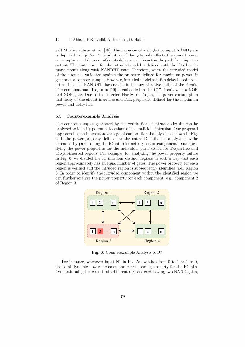
12 I. Abbasi, F.K. Lodhi, A. Kamboh, O. Hasan
and Mukhopadhyay et. al. [19]. The intrusion of a single two input NAND gateis depicted in Fig. 5a . The addition of the gate only a↵ects the overall powerconsumption and does not a↵ect its delay since it is not in the path from input tooutput. The state space for the intruded model is defined with the C17 bench-mark circuit along with NANDHT gate. Therefore, when the intruded modelof the circuit is validated against the property defined for maximum power, itgenerates a counterexample. However, intruded model satisfies delay based prop-erties since the NANDHT does not lie in the any of active paths of the circuit.The combinational Trojan in [19] is embedded in the C17 circuit with a NORand XOR gate. Due to the inserted Hardware Trojan, the power consumptionand delay of the circuit increases and LTL properties defined for the maximumpower and delay fails.
5.5 Counterexample Analysis
The counterexamples generated by the verification of intruded circuits can beanalyzed to identify potential locations of the malicious intrusion. Our proposedapproach has an inherent advantage of compositional analysis, as shown in Fig.6. If the power property defined for the entire IC fails, the analysis may beextended by partitioning the IC into distinct regions or components, and spec-ifying the power properties for the individual parts to isolate Trojan-free andTrojan-inserted regions. For example, for analyzing the power property failurein Fig. 6, we divided the IC into four distinct regions in such a way that eachregion approximately has an equal number of gates. The power property for eachregion is verified and the intruded region is subsequently identified, i.e., Region3. In order to identify the intruded component within the identified region wecan further analyze the power property for each component, e.g., component 2of Region 3.
Fig. 6: Counterexample Analysis of IC
For instance, whenever input N1 in Fig. 5a switches from 0 to 1 or 1 to 0,the total dynamic power increases and corresponding property for the IC fails.On partitioning the circuit into di↵erent regions, each having two NAND gates,
79
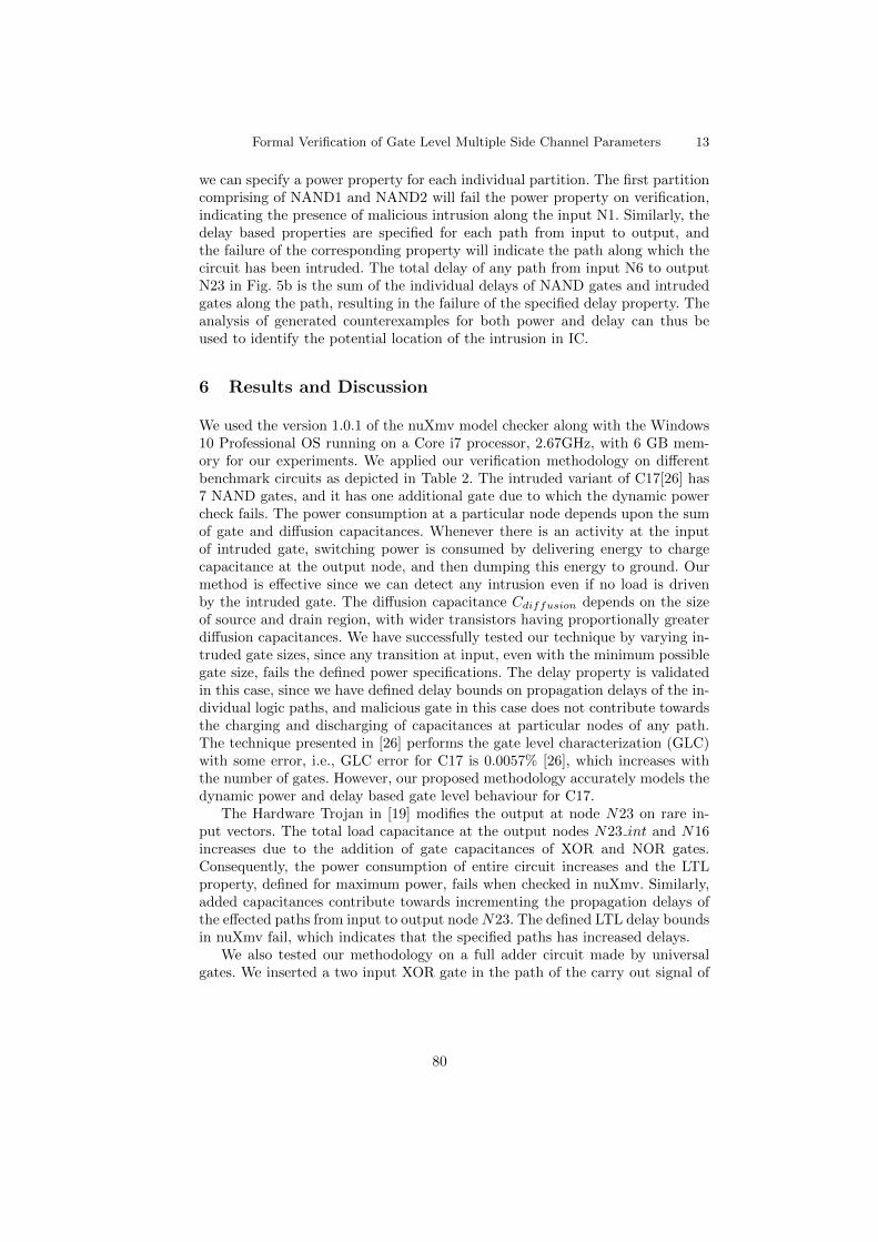
Formal Verification of Gate Level Multiple Side Channel Parameters 13
we can specify a power property for each individual partition. The first partitioncomprising of NAND1 and NAND2 will fail the power property on verification,indicating the presence of malicious intrusion along the input N1. Similarly, thedelay based properties are specified for each path from input to output, andthe failure of the corresponding property will indicate the path along which thecircuit has been intruded. The total delay of any path from input N6 to outputN23 in Fig. 5b is the sum of the individual delays of NAND gates and intrudedgates along the path, resulting in the failure of the specified delay property. Theanalysis of generated counterexamples for both power and delay can thus beused to identify the potential location of the intrusion in IC.
6 Results and Discussion
We used the version 1.0.1 of the nuXmv model checker along with the Windows10 Professional OS running on a Core i7 processor, 2.67GHz, with 6 GB mem-ory for our experiments. We applied our verification methodology on di↵erentbenchmark circuits as depicted in Table 2. The intruded variant of C17[26] has7 NAND gates, and it has one additional gate due to which the dynamic powercheck fails. The power consumption at a particular node depends upon the sumof gate and di↵usion capacitances. Whenever there is an activity at the inputof intruded gate, switching power is consumed by delivering energy to chargecapacitance at the output node, and then dumping this energy to ground. Ourmethod is e↵ective since we can detect any intrusion even if no load is drivenby the intruded gate. The di↵usion capacitance Cdiffusion depends on the sizeof source and drain region, with wider transistors having proportionally greaterdi↵usion capacitances. We have successfully tested our technique by varying in-truded gate sizes, since any transition at input, even with the minimum possiblegate size, fails the defined power specifications. The delay property is validatedin this case, since we have defined delay bounds on propagation delays of the in-dividual logic paths, and malicious gate in this case does not contribute towardsthe charging and discharging of capacitances at particular nodes of any path.The technique presented in [26] performs the gate level characterization (GLC)with some error, i.e., GLC error for C17 is 0.0057% [26], which increases withthe number of gates. However, our proposed methodology accurately models thedynamic power and delay based gate level behaviour for C17.
The Hardware Trojan in [19] modifies the output at node N23 on rare in-put vectors. The total load capacitance at the output nodes N23 int and N16increases due to the addition of gate capacitances of XOR and NOR gates.Consequently, the power consumption of entire circuit increases and the LTLproperty, defined for maximum power, fails when checked in nuXmv. Similarly,added capacitances contribute towards incrementing the propagation delays ofthe e↵ected paths from input to output node N23. The defined LTL delay boundsin nuXmv fail, which indicates that the specified paths has increased delays.
We also tested our methodology on a full adder circuit made by universalgates. We inserted a two input XOR gate in the path of the carry out signal of
80
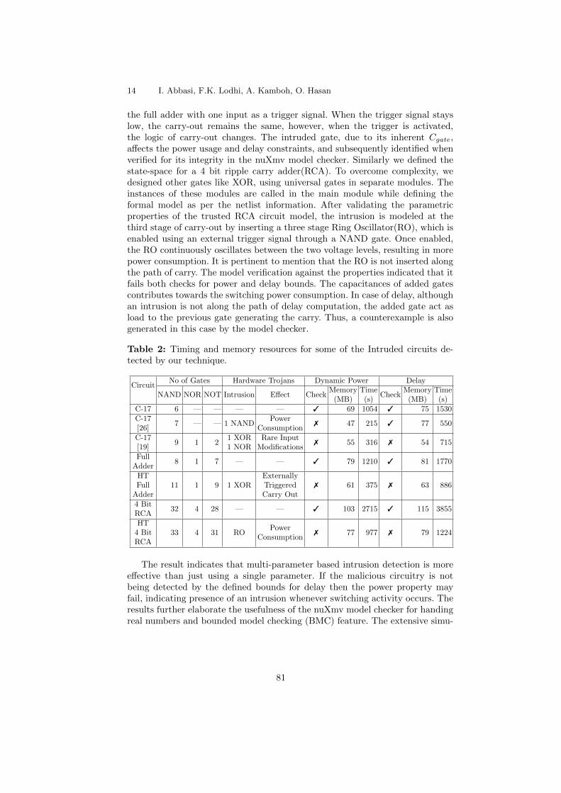
14 I. Abbasi, F.K. Lodhi, A. Kamboh, O. Hasan
the full adder with one input as a trigger signal. When the trigger signal stayslow, the carry-out remains the same, however, when the trigger is activated,the logic of carry-out changes. The intruded gate, due to its inherent Cgate,a↵ects the power usage and delay constraints, and subsequently identified whenverified for its integrity in the nuXmv model checker. Similarly we defined thestate-space for a 4 bit ripple carry adder(RCA). To overcome complexity, wedesigned other gates like XOR, using universal gates in separate modules. Theinstances of these modules are called in the main module while defining theformal model as per the netlist information. After validating the parametricproperties of the trusted RCA circuit model, the intrusion is modeled at thethird stage of carry-out by inserting a three stage Ring Oscillator(RO), which isenabled using an external trigger signal through a NAND gate. Once enabled,the RO continuously oscillates between the two voltage levels, resulting in morepower consumption. It is pertinent to mention that the RO is not inserted alongthe path of carry. The model verification against the properties indicated that itfails both checks for power and delay bounds. The capacitances of added gatescontributes towards the switching power consumption. In case of delay, althoughan intrusion is not along the path of delay computation, the added gate act asload to the previous gate generating the carry. Thus, a counterexample is alsogenerated in this case by the model checker.
Table 2: Timing and memory resources for some of the Intruded circuits de-tected by our technique.
CircuitNo of Gates Hardware Trojans Dynamic Power Delay
NAND NOR NOT Intrusion E↵ect CheckMemory(MB)
Time(s)
CheckMemory(MB)
Time(s)
C-17 6 — — — — 3 69 1054 3 75 1530C-17[26]
7 — — 1 NANDPower
Consumption7 47 215 3 77 550
C-17[19]
9 1 21 XOR1 NOR
Rare InputModifications
7 55 316 7 54 715
FullAdder
8 1 7 — — 3 79 1210 3 81 1770
HTFull
Adder11 1 9 1 XOR
ExternallyTriggeredCarry Out
7 61 375 7 63 886
4 BitRCA
32 4 28 — — 3 103 2715 3 115 3855
HT4 BitRCA
33 4 31 ROPower
Consumption7 77 977 7 79 1224
The result indicates that multi-parameter based intrusion detection is moree↵ective than just using a single parameter. If the malicious circuitry is notbeing detected by the defined bounds for delay then the power property mayfail, indicating presence of an intrusion whenever switching activity occurs. Theresults further elaborate the usefulness of the nuXmv model checker for handingreal numbers and bounded model checking (BMC) feature. The extensive simu-
81
Formal Verification of Gate Level Multiple Side Channel Parameters 15
lations for every possible input using traditional methods is a laborious task. Incontrast, once a model is defined in a model checker based on the proposed ap-proach, then it takes significantly lesser time and resources to test the integrityof the entire system. The results in Table 2 show that modeling and verificationof all the case studies require a 115MB of memory at maximum, which is around2% of the available memory of the machine used to acquire these experimentalresults. Therefore, the proposed approach seems quite scalable to handle largercircuits with the availability of around 16GB memory. However, the inherentstate-space explosion problem of model checking may limit the applicability ofthe proposed approach for larger circuits and therefore, in these cases, we planto extend the models to a higher abstraction level.
7 Comparison with Existing Gate Modeling Techniques
The gate level time and power models have been presented previously by dif-ferent researchers. The timing analysis at the gate level description of a circuitis proposed in [4], where each gate is abstracted as a set of states and indi-vidual transitions are characterized by the propagation delay of the falling orrising edge. The propagation delays are determined by using set of di↵erentialequations for capacitances or through SPICE simulations. Timing verificationfor asynchronous circuits, proposed in [7], is based on translating the circuitbehavior in terms of transition graphs, which is checked under the assumptionthat the delays are bounded between two numbers. The formal verification oftimed circuits is represented as symbols with unspecified delays in [11]. In thisscheme, a set of linear constraints on the symbols are discovered that guaranteesthe correctness of the circuit. Similarly, a state transition graph based powerdissipation model is presented in [16] that considers charging and discharging ofthe capacitance at the gate output node. The input signal probabilities are usedto estimate the expected activity number of each edge in the graph, followedby computing the total consumption by summing each edge. The consumptionvalues of transitions are obtained from SPICE simulation.
The proposed gate modeling technique in this paper takes both power andtiming parameters under consideration. Our scheme has an inherent advantagein the perspective of hardware intrusion detection that we take particular VLSItechnology and possible variations in fanout and gate sizes in to account as well.Moreover, our model is generic as we estimate power and timing measurementswith all possible input transitions without any requirements of simulations withSPICE or other circuit simulators.
8 Conclusions
This paper presents a generic framework based on the formal verification ofthe integrated circuit (IC) to detect malicious hardware intrusions. Unlike thetraditional methods to detect the intrusions in integrated circuits, our solutionuses formal models based on multi-parameter side channel information and their
82
16 I. Abbasi, F.K. Lodhi, A. Kamboh, O. Hasan
validation using a model checker. The ability of nuXmv model checker to handlereal numbers and the powerful verification methods, based on SAT and SMTsolvers, has been successfully utilized to validate dynamic power and path delayparameters, to ascertain integrity of integrated circuits. In the future, we plan toenhance this work by proposing an automated method for netlist translation, andextending the models to higher abstraction level to e�ciently handle scalabilityfor larger ICs. Moreover, additional side channel parameters, such as leakagepower will also be incorporated in order to strengthen the proposed HardwareTrojan detection scheme.
References
1. Adee, S.: The Hunt for the Kill Switch. IEEE Spectrum 45(5), 34–39 (2008)2. Agrawal, D., Baktir, S., Karakoyunlu, D., Rohatgi: Trojan Detection using IC
Fingerprinting. In: Symposium on Security and Privacy. pp. 296–310. IEEE (2007)3. Anderson, M.S., North, C., Yiu, K.K.: Towards Countering the Rise of the Silicon
trojan. Defence Science and Technology Organisation, DSTO-TR-2220, Australia(2008)
4. Bara, A., Bazargan-Sabet, P., Chevallier, R., Encrenaz: Formal Verification ofTimed VHDL Programs. In: Specification & Design Languages. pp. 1–6. IET (2010)
5. Bhasin, S., Regazzoni, F.: A Survey on Hardware Trojan Detection Techniques.In: Circuits and Systems. pp. 2021–2024. IEEE (2015)
6. Bhunia, S., Hsiao, M.S., Banga, M., Narasimhan, S.: Hardware Trojan Attacks:Threat Analysis and Countermeasures. vol. 102, pp. 1229–1247. IEEE (2014)
7. Bozga, M., Jianmin, H., Maler: Verification of Asynchronous Circuits using TimedAutomata. Electronic Notes in Theoretical Computer Science 65(6), 47–59 (2002)
8. Cavada, R., Cimatti, A., Dorigatti, M., Griggio, A., Mariotti, A., Micheli, A.,Mover, S., Roveri, M., Tonetta, S.: The nuXmv Symbolic Model Checker. In: Com-puter Aided Verification, LNCS, vol. 8559, pp. 334–342. Springer (2014)
9. Chakraborty, R.S., Wol↵, F., Paul, S., Papachristou, C., Bhunia, S.: MERO: AStatistical Approach for Hardware Trojan Detection. In: Cryptographic Hardwareand Embedded Systems, pp. 396–410. Springer (2009)
10. Cimatti, A., Clarke, E., Giunchiglia, E., Giunchiglia, F., Pistore, M., Roveri, M.,Sebastiani: NuSMV 2: An Opensource Tool for Symbolic Model Checking. In:International Conference on Computer Aided Verification. pp. 359–364. Springer(2002)
11. Clariso, R., Cortadella, J.: Verification of Timed Circuits with Symbolic Delays. In:Asia and South Pacific Design Automation Conference. pp. 628–633. IEEE (2004)
12. Di Natale, G., Dupuis: Is Side-Channel Analysis Really Reliable for DetectingHardware Trojans? In: Design of Circuits and Integrated Systems. pp. 238–242(2012)
13. Drechsler, R., et al.: Advanced Formal Verification. No. ISBN 9781402077210,Springer (2004)
14. Force, T.: High Performance Microchip Supply. Defense Technical InformationCenter (DTIC), USA (2005), http://www.acq.osd.mil/dsb/reports/ADA435563.pdf
15. Jin, Y., Makris, Y.: Hardware Trojan Detection using Path Delay Fingerprint. In:Hardware-Oriented Security and Trust, 2008. pp. 51–57. IEEE (2008)
83
Formal Verification of Gate Level Multiple Side Channel Parameters 17
16. Lin, J.Y., Liu, T.C., Shen, W.Z.: A Cell-Based Power Estimation in CMOS Com-binational Circuits. In: Computer-Aided Design. pp. 304–309. IEEE (1994)
17. MathSAT 5: (2016), http://mathsat.fbk.eu/18. Mitra, S., Wong, H.S.P., Wong, S.: The Trojan-Proof Chip. IEEE Spectrum 52(2),
46–51 (2015)19. Mukhopadhyay, D., Chakraborty, R.S.: Hardware Security: Design, Threats, and
Safeguards. No. ISBN 9781439895832, CRC (2014)20. Qu, G., Yuan, L.: Design THINGS for the Internet of Things-An EDA Perspective.
In: International Conference on Computer-Aided Design (ICCAD). pp. 411–416.IEEE (2014)
21. Rabaey, J.M., Chandrakasan, A.P., Nikolic, B.: Digital Integrated Circuits, vol. 2.Prentice hall (2002)
22. Rai, D., Lach, J.: Performance of Delay-Based Trojan Detection under ParameterVariations. In: Hardware-Oriented Security and Trust. pp. 58–65. IEEE (2009)
23. Rathmair, M., Schupfer, F.: Hardware Trojan Detection by Specifying MaliciousCircuit Properties. In: Electronics Information and Emergency Communication.pp. 317–320. IEEE (2013)
24. Tehranipoor, M., Koushanfar, F.: A Survey of Hardware Trojan Taxonomy andDetection. IEEE Design and Test of Computers 27(1), 10–25 (2010)
25. Wang, L., Xie, H., Luo, H.: Malicious Circuitry Detection using Transient PowerAnalysis for IC Security. In: Quality, Reliability, Risk, Maintenance, and SafetyEngineering. pp. 1164–1167. IEEE (2013)
26. Wei, S., Meguerdichian, S., Potkonjak, M.: Malicious Circuitry Detection usingThermal Conditioning. IEEE Transactions on Information Forensics and Security6(3), 1136–1145 (2011)
27. Weste, N., Harris, D.: CMOS VLSI Design: A Circuits and Systems Perspective.No. ISBN 9780321547743, Pearson (2011)
28. Xiao, K., Forte, D., Jin, Y., Karri, R., Bhunia, S., Tehranipoor, M.: HardwareTrojans: Lessons Learned After One Decade of Research. ACM Transactions onDesign Automation of Electronic Systems Vol 22(1) (2016)
29. Zhang, X., Tehranipoor, M.: Detecting Hardware Trojans in Third-Party DigitalIP Cores. In: Hardware-Oriented Security and Trust (HOST). pp. 67–70. IEEE(2011)
84
Formal Probabilistic Analysis of a WSN-basedMonitoring Framework for IoT Applications
Maissa Elleuch1,3, Osman Hasan2, Sofiene Tahar2, and Mohamed Abid1
1 CES Laboratory, National School of Engineers of Sfax, Sfax UniversitySoukra Street, 3052 Sfax, [email protected]
[email protected] Dept. of Electrical & Computer Engineering, Concordia University
1455 de Maisonneuve W., Montreal, Quebec, H3G 1M8, Canada{melleuch,o hasan,tahar}@ece.concordia.ca
3 Digital Research Center of SfaxTechnopark of Sfax, Tunisia
Abstract. Internet of Things (IoT) has been considered as an intuitiveevolution of sensing systems using Wireless Sensor Networks (WSN). Inthis context, energy e�ciency is considered as one of the most critical re-quirement. For that purpose, the randomized node scheduling approachis largely applied. The randomness feature in the node scheduling to-gether with the unpredictable deployment make probabilistic techniquesmuch more appropriate to evaluate the coverage properties of WSNs.Classical probabilistic analysis techniques, such as simulation and modelchecking, do not guarantee accurate results, and thus are not suitable foranalyzing mission-critical WSN applications. Based on the most recentlydeveloped probability theory, available in the HOL theorem prover, wedevelop the formalizations of the key coverage performance attributes:the coverage intensity of a specific point and the expected value of thenetwork coverage intensity. The practical interest of our higher-order-logic developments is finally illustrated through formally analyzing theasymptotic coverage behavior of an hybrid monitoring framework forenvironmental IoT.
Keywords: Theorem proving, Wireless sensor networks, node schedul-ing, performance analysis, network coverage, environmental monitoring
1 Introduction
Wireless Sensor Networks (WSN) have emerged as a key enabler technology forthe development of the Internet of Things (IoT) paradigm [20,24]. Deployed overa field of interest, smart sensor nodes collaborate together without any humaninteraction, in order to mainly achieve a monitoring or a tracking task. Suchnetworks are covering limitless applications [28], including home automation,external environmental monitoring and object tracking, and hence integratingWSN technologies into the IoT context [20,12].
85
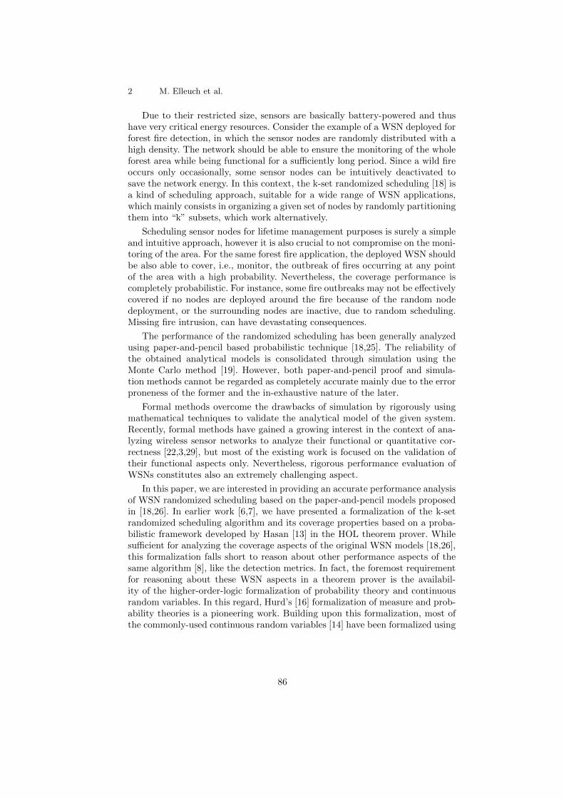
2 M. Elleuch et al.
Due to their restricted size, sensors are basically battery-powered and thushave very critical energy resources. Consider the example of a WSN deployed forforest fire detection, in which the sensor nodes are randomly distributed with ahigh density. The network should be able to ensure the monitoring of the wholeforest area while being functional for a su�ciently long period. Since a wild fireoccurs only occasionally, some sensor nodes can be intuitively deactivated tosave the network energy. In this context, the k-set randomized scheduling [18] isa kind of scheduling approach, suitable for a wide range of WSN applications,which mainly consists in organizing a given set of nodes by randomly partitioningthem into “k” subsets, which work alternatively.
Scheduling sensor nodes for lifetime management purposes is surely a simpleand intuitive approach, however it is also crucial to not compromise on the moni-toring of the area. For the same forest fire application, the deployed WSN shouldbe also able to cover, i.e., monitor, the outbreak of fires occurring at any pointof the area with a high probability. Nevertheless, the coverage performance iscompletely probabilistic. For instance, some fire outbreaks may not be e↵ectivelycovered if no nodes are deployed around the fire because of the random nodedeployment, or the surrounding nodes are inactive, due to random scheduling.Missing fire intrusion, can have devastating consequences.
The performance of the randomized scheduling has been generally analyzedusing paper-and-pencil based probabilistic technique [18,25]. The reliability ofthe obtained analytical models is consolidated through simulation using theMonte Carlo method [19]. However, both paper-and-pencil proof and simula-tion methods cannot be regarded as completely accurate mainly due to the errorproneness of the former and the in-exhaustive nature of the later.
Formal methods overcome the drawbacks of simulation by rigorously usingmathematical techniques to validate the analytical model of the given system.Recently, formal methods have gained a growing interest in the context of ana-lyzing wireless sensor networks to analyze their functional or quantitative cor-rectness [22,3,29], but most of the existing work is focused on the validation oftheir functional aspects only. Nevertheless, rigorous performance evaluation ofWSNs constitutes also an extremely challenging aspect.
In this paper, we are interested in providing an accurate performance analysisof WSN randomized scheduling based on the paper-and-pencil models proposedin [18,26]. In earlier work [6,7], we have presented a formalization of the k-setrandomized scheduling algorithm and its coverage properties based on a proba-bilistic framework developed by Hasan [13] in the HOL theorem prover. Whilesu�cient for analyzing the coverage aspects of the original WSN models [18,26],this formalization falls short to reason about other performance aspects of thesame algorithm [8], like the detection metrics. In fact, the foremost requirementfor reasoning about these WSN aspects in a theorem prover is the availabil-ity of the higher-order-logic formalization of probability theory and continuousrandom variables. In this regard, Hurd’s [16] formalization of measure and prob-ability theories is a pioneering work. Building upon this formalization, most ofthe commonly-used continuous random variables [14] have been formalized using
86
Formal Probabilistic Analysis of a WSN-based Monitoring Framework 3
the HOL theorem prover. However, this foundational formalization of probabilitytheory only supports the whole universe as the probability space, which limitsits scope in many aspects. In particular the inability to reason about multiplecontinuous random variables [14] is a major obstacle for modeling and analyzingdetection and lifetime properties of WSNs [9]. More recent probability theoryformalizations [21,15], however, allow the use of any arbitrary probability spacethat is a subset of the universe and thus are more flexible than Hurd’s andHasan’s formalizations of probability theory. Particularly, Mhamdi’s [21] proba-bility theory formalization which is based on extended-real numbers (real num-bers including ±1), has been included in the HOL theorem prover and thus hasbeen chosen for our work. Therefore, in this paper we propose to use the mostrecent probability theory developed by Mhamdi [21] in HOL to formally reasonabout the coverage properties of randomly-scheduled WSN, while emphasizingon the main lessons learned through this experience. The practical interest of thenew developments is illustrated through the formal analysis of the asymptoticcoverage behavior of a WSN based environmental surveillance framework.
The rest of this paper is organized as follows. We review some related workon the validation of WSNs in Section 2. In Section 3, we summarize the mainrequirements of this work. Section 4 provides the foundational probabilistic anal-ysis of the coverage properties. We utilize these developments to formally verifya WSN-based monitoring framework for IoT applications in Section 5. Section 6is devoted to discuss the main results of our work. We finally conclude the paperin Section 7.
2 Related Work
Theoretical analysis, also known as paper-and-pencil based probabilistic tech-nique, has been widely used to validate randomized scheduling algorithms forWSN [18,25,26]. Such analysis consists in constructing a theoretical model wherethe required random variables are determined together with the associated per-formance metrics. Afterwards, a probabilistic based study is achieved. For vali-dation purposes, simulation, using the Monte Carlo method [19], is finally done.
Traditional model checking technique [2] has been successfully used to val-idate various aspects in the WSN context. In [22], the formal analysis of theOptimal Geographical Density Control (OGDC) algorithm, which is a kind ofrandomized scheduling algorithm, is done. Several other prominent works re-ported on the use of model checking for the analysis of WSN protocols include[10,30]. The main strength of all these methods is their formal models and auto-matic verification. However, they su↵er from the common model checking relatedproblem of state space explosion [2]. Hence, the analysis of the OGDC algorithm[22] has been restricted for WSN with up to 6 nodes in a region of 15m ⇥ 15m.Furthermore, the work of [30] has pointed out over 1 million generated states forthe analysis of a simple property. Furthermore, none of the previous works hasprovided reliable probabilistic modelling. For example, in [22], a random func-tion, assumed to be ’good’, has been used to model the probabilistic behavior.
87
4 M. Elleuch et al.
To cope with these major problems, probabilistic model checking [23] hasalso been used for the probabilistic functional analysis of wireless systems. Prob-abilistic model checking allows to capture the probability modelling for both thesystem and the property of interest. The probabilistic model checker PRISMhas been applied quite frequently for the validation of Medium Access Control(MAC) protocols for WSNs [11,29]. Nevertheless, the reasoning support for sta-tistical quantities in most of model checkers su↵ers from many shortcomings.Indeed, expected performance values are usually obtained through several runson the built model [29]. The obtained results can hardly be termed as exhaustiveand thus formally verified.
On the other hand, very few works based on theorem proving exist in theopen literature. The work [4] reports on the use of the PVS system to builda theorem proving based framework for WSN algorithms, with some theoriesexpressing dynamic scenarios like nodes mobility and link quality changes [4].While the PVS framework is supposed to be extended with some “dynamic”scenarios in [4], the randomness aspect has been characterized by a pseudo-random generator. The nodes mobility, specified by the random walk pattern,has been also specified through a recursive function.
Unlike the PVS framework which is limited by the probability support of thePVS system, the work, described in this paper, provides very accurate formal-izations of the randomized scheduling algorithm based on the sound probabilitysupport of the HOL theorem prover. In addition, the presented formalizationsare generic and completely valid for all the parameter values.
3 Preliminaries
3.1 Probabilistic Analysis in HOL
A probability measure P is basically a measure function on the sample space ⌦and an event is a measurable set within the set F of events which are subsetsof ⌦. By definition, a random variable is a measurable function, satisfying thecondition that the inverse image of a measurable set is also measurable [21].
Definition 1. ` 8X p. real random variable X p =
prob space p ^(8x 2 p space p ) X x 6= NegInf ^ X x 6= PosInf) ^X 2 measurable (p space p,events p) Borel.
where X designates the random variable, p is a given probability space, NegInfand PosInf are the higher-order-logic formalizations of negative infinity or pos-itive infinity, and Borel is the HOL definition of the Borel sigma algebra.
The probability distribution of a random variable is specified as the functionthat accepts a random variable X and a set s and returns the probability of theevent {X 2 s}.
Definition 2. ` 8X p.
distribution p X = (�s. prob p (PREIMAGE X s \ p space p)).
88
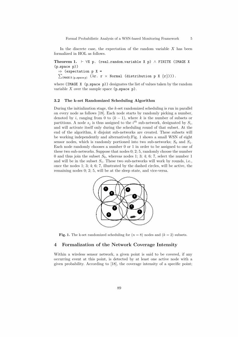
Formal Probabilistic Analysis of a WSN-based Monitoring Framework 5
In the discrete case, the expectation of the random variable X has beenformalized in HOL as follows.
Theorem 1. ` 8X p. (real random variable X p) ^ FINITE (IMAGE X
(p space p))
) (expectation p X =PIMAGE X (p space p) (�r. r ⇥ Normal (distribution p X {r}))).
where (IMAGE X (p space p)) designates the list of values taken by the randomvariable X over the sample space (p space p).
3.2 The k-set Randomized Scheduling Algorithm
During the initialization stage, the k-set randomized scheduling is run in parallelon every node as follows [18]. Each node starts by randomly picking a number,denoted by i, ranging from 0 to (k � 1), where k is the number of subsets orpartitions. A node sj is thus assigned to the ith sub-network, designated by Si,and will activate itself only during the scheduling round of that subset. At theend of the algorithm, k disjoint sub-networks are created. These subsets willbe working independently and alternatively.Fig. 1 shows a small WSN of eightsensor nodes, which is randomly portioned into two sub-networks; S0 and S1.Each node randomly chooses a number 0 or 1 in order to be assigned to one ofthese two sub-networks. Suppose that nodes 0; 2; 5, randomly choose the number0 and thus join the subset S0, whereas nodes 1; 3; 4; 6; 7, select the number 1and will be in the subset S1. These two sub-networks will work by rounds, i.e.,once the nodes 1; 3; 4; 6; 7, illustrated by the dashed circles, will be active, theremaining nodes 0; 2; 5, will be at the sleep state, and vice-versa.
Fig. 1. The k-set randomized scheduling for (n = 8) nodes and (k = 2) subsets.
4 Formalization of the Network Coverage Intensity
Within a wireless sensor network, a given point is said to be covered, if anyoccurring event at this point, is detected by at least one active node with agiven probability. According to [18], the coverage intensity of a specific point;
89
6 M. Elleuch et al.
Cp, inside the monitored area is defined as the average time during which thepoint is covered in a whole scheduling cycle of length k ⇥ T . A given point iscovered if the current active subset contains at least one node, i.e., is not empty.
Let X be the random variable describing the total number of non-emptysubsets, the coverage intensity of a given point in the monitored area, Cp, asoriginally specified in [18], is
Cp =E[X] ⇥ T
k ⇥ T. (1)
where E[X] denotes the expectation of X, which is described as:
X =k�1X
j=0
Xj . (2)
where Xj is the Bernoulli random variable whose value is 1 in case of non-empty subset. A non-empty sub-network is described by a Bernoulli randomvariable with the complement probability of
�1� 1
k
�c[6], where c is the number
of covering sensors for a given point.
Definition 3. ` 8X p k c.
sbst non empty rv X p k c = bernoulli distr rv X p�1�
�1� 1
&k
�c�.
In higher-order logic, we model the coverage behavior of a specific point(Equation (1)) by the following predicate cvrge intsty pt.
Definition 4. ` 8p X k s c. cvrge intsty pt p X k s c =
expectation p (�x. SIGMA (�i. (X i) x) s) / (&k).
where X: a random variable that returns an extended real number, p: the prob-ability space, k: the number of sub-networks, s: the summation set whose cardi-nality is k, and c: the number of covering sensors for a given point. The operator& allows the conversion of the natural number m into its extended real numbercounterpart.
The following mathematical expression for the coverage intensity of a pointhas been formally verified in Theorem 2.
Theorem 2. ` 8X p k s c. (prob space p) ^ (FINITE s) ^ (1 < k)
^ (CARD s = k) ^ (8i. i 2 s ) sbst non empty rv (X i) p k c)
) (cvrge intsty pt p X k s pr = Normal�1�
�1� 1
k
�c�).
– The assumption (8i. i 2 s ) sbst non empty rv (X i) p k c) indi-cates that every element of the set s is a random variable sbst non empty rv
(Definition 3).
– The HOL function Normal is used to convert a real value to its correspondingvalue in an extended real.
90
Formal Probabilistic Analysis of a WSN-based Monitoring Framework 7
The proof of the above theorem is mainly based on lemmas about the linearityof the expectation property, which in turn required some reasoning on the inte-grability of some functions as well as operations from the Lebesgue theory. Formost of these lemmas, it was a prerequisite to verify the measurability of theused events, along with some analysis on extended reals.
The whole network can be now statistically described by a single performancemetric; Cn, which is the average or the expectation value of the coverage intensityover all points of the monitored area.
Cn = E[Cp] . (3)
According to the expression of Cp, shown in Theorem 2, we can write
Cn = E[1 �✓
1 � 1
k
◆c
] . (4)
Based on the above equation, we notice how the value of Cn depends mainlyon c which is the number of nodes covering a given point of the field. Intuitively,we can assimilate the fact of covering a point or not to a Bernoulli trial withthe probability q = r
a [18]. Considering the variable c among the n nodes of thenetwork, it becomes a Binomial random variable (C) with the probability givenin Equation (5). Thereby, the network coverage intensity Cn, shown in Equation(4), is not a simple expectation, but rather an expectation of a function of arandom variable.
Pr(C = j) = Cjn ⇥
⇣ r
a
⌘j
⇥⇣1 �
⇣ r
a
⌘⌘n�j
. (5)
where Cjn is the binomial coe�cient, r is the size of the sensing area of each
sensor, a is the size of the monitored area, and�
ra
�is the probability that each
sensor covers a given point. The Binomial random variable with n trials andsuccess probability q =
�ra
�has been formalized in HOL as follows.
Definition 5. ` 8X p q n. binomial distr rv X p q n =
(real random variable X p) ^(IMAGE X (p space p) = IMAGE (�x.&x) (count (SUC n))) ^(8m. &m 2 (IMAGE X (p space p)) )(distribution p X {&m} = &(binomial n m) ⇥ qm ⇥ (1� q)(n�m)).
where X is a real random variable on the probability space p, and IMAGE (�x.&x)(count (SUC n)) gives the support of the Binomial. The function binomial,used in the above definition, is the higher-order-logic formalization of the bino-mial coe�cient for reals.
The coverage intensity of the whole WSN with n nodes has been formallyspecified by the function cvrge intsty network, shown in Definition 6. Thelatter takes as parameters: X: a random variable that returns an extended realnumber, p: the probability space, s: the summation set used in Definition 4, k:the number of sub-networks, C: the random variable describing the number of
91

8 M. Elleuch et al.
covering nodes, n: the total number of nodes, and q: the probability that eachsensor covers a given point.
Definition 6. ` 8X p k s C n q.
cvrge intsty network p X k s C n q =
expectation p (�x. cvrge intsty pt p X k s (num (C x))).
where the function expectation designates the higher-order-logic formalizationof the expectation of a random variable that returns an extended real, and thevalues (num(C x)), in the above definition, are the output values of the randomvariable C. The function num, used here, converts an extended real; (&m), to itscorresponding natural value m, using the real function floor.
Based on the higher-order-logic formalizations developed so far, we have beenable to formally verify the final network coverage intensity as in Theorem 3.
Theorem 3. ` 8p X k s C n q. (prob space p) ^ (0 < q < 1) ^(events p = POW (p space p)) ^ (1 n) ^ (1 < k) ^ FINITE s ^(CARD s = k) ^ (sn covers p C p q n) ^(expectation p C 6= PosInf) ^ (expectation p C 6= NegInf) ^(8i x. (i 2 s) ^ (x 2 p space p) )
sbst non empty rv (X i) p k (num(C x)))
) (cvrge intsty network p X k s C n q = Normal (1� (1� q(&k) )
n)).
– The assumption (events p = POW (p space p)) describes the set of eventsto be the power set of the sample space ⌦.
– The assumptions (1 n) ensures that the WSN include at least one node,while (0 < q < 1) checks that the probability q lies in [0..1].
– sn covers p is the Binomial random variable (Definition 5) with a finiteexpectation, i.e., (expectation p C 6= PosInf) ^ (expectation p C 6=NegInf). The variables (PosInf) and (NegInf) are the higher-order-logicformalizations of positive infinity and negative infinity, respectively.
– The function (sbst non empty rv (X i) p k (num(C x))) is the functionspecified in Definition 3.
The proof of Theorem 3 is primarily based on Theorem 4 which verifies theexpectation of a function of a random variable. Additionally, the current proofalso required the application of the linearity of the expectation property. Finally,a considerable amount of real analysis associated to the Binomial theorem forreals, and to the summation function has been needed.
Theorem 4. ` 8C p q n k.
(prob space p) ^ (1 < k) ^ (0 < q < 1) ^(events p = POW (p space p)) ^ (1 n) ^ (sn covers p C p q n)
) (expectation p (�x. f fct (num (C x)) k) = Normal (1� q(&k) )
n).
where the function f fct is defined as follows
f fct x k = Normal
✓1� 1
k
◆x
. (6)
92
Formal Probabilistic Analysis of a WSN-based Monitoring Framework 9
The proof of Theorem 4 has been possible using intermediate results on theinjectivity of some functions, as well as, some properties related to the randomvariables functions. A lot of reasoning associated with the use of extended realand the floor function, has also been required.
In this section, we presented our new higher-order-logic formalizations ofthe k-set randomized scheduling for wireless sensor networks, using the recentlydeveloped probability theory available in the HOL theorem prover [21]. Theseformalizations have been then utilized to formally reason about the coverageperformance properties. The corresponding HOL code of the current formaliza-tions is available at [5]. Due to fundamental di↵erences in the foundations of thetwo probability theories in [13] and [21], the current resulting formalizations iscompletely di↵erent from the previous one [6]. Indeed, the new probability the-ory allows to cater for arbitrary probability spaces and is thus more generic andcomplete compared to the previous formalization in which the probability spacehas to be the universe of a set. Moreover, the specification of the randomizedalgorithm has been found to be much more intuitive with [21]. Unlike the workin [6], the developed proofs required much less reasoning about sets and lists pro-ducing thus less lengthy proofs. However, these proofs have been more labouredinvolving usually results from the three HOL theories: Lebesgue, measure andextended reals. A deep learning of all theoretical foundations of [21] was thusrequired to successfully achieve the target formalizations in the HOL theoremprover. In the next section, we will illustrate how the developed generic theoremsextremely facilitate the formal analysis of real-world WSN applications.
5 Application: Formal Analysis of a WSN-basedmonitoring framework for IoT Applications
Numerous frameworks for environmental monitoring based on WSN have beenhence proposed in the literature [1,27]. These systems can be seamlessly inte-grated to build an extended IoT framework for low-cost, persistent and e�cientservices [17,12]. Due to the new constraints of the IoT environment, deployedWSN should have a smart behavior regarding the power availability while per-forming a good coverage of any intrusion. The randomized node scheduling hasbeen proposed for use to save energy in the context of an heterogeneous surveil-lance framework for environmental monitoring [27]. Such framework considerscollaboration between sensor nodes, mobile robots and RFID tags, to ensure ef-ficient surveillance. Using specific sensors designed for IoT [17], this frameworkcan realize a whole IoT structure.
In this section, we focus on formally analyzing the coverage performances ofthe hybrid surveillance framework proposed in [27] adopted for IoT applications.The nodes can hence have any sensing area r, and are deployed into a circularregion of a radius R with a total size of a, whereas the success probability q ofa sensor covering a point is q = r
a . Such framework has been primarily analyzedusing a paper-and-pencil model, which has been then validated through somesimulation scenarios evaluating the expected coverage and the maximum number
93
10 M. Elleuch et al.
of subsets [27]. It would be interesting to provide a more rigorous technique tovalidate the proposed paper-and-pencil model. Based on the formal developmentachieved so far, we show in this section how we are able to carry out an accurateasymptotic analysis of the probabilistic coverage according to the key designparameters: n; the total number of sensor and k; the number of subsets.
We designate the generic network coverage intensity (cvrge intsty network
p X s k C n q), shown in Definition 6, by (Cn wsn p X s k C n q), that hasbeen checked in HOL as
Normal⇣1�
⇣1� q
k
⌘n⌘. (7)
5.1 Formal Analysis based on the Number of Nodes
Setting the number of subsets to k and targeting a network coverage intensityCn wsn of at least t, we verify, in Lemma 1, the minimum number of sensors;nmin, that are necessary to deploy in the context of our monitoring framework.
Lemma 1. ` 8p X s k C n q t. (1 n) ^ (1 < k) ^ (0 < q < 1) ^(0 < t < 1) ^ (Normal t Cn wsn p X s k C n q)
)
ln(1�t)
ln(1� qk )
� &n.
The higher-order-logic proof of the above lemma is based on some properties oftranscendental functions and arithmetic reasoning.
We have been able to formally verify, in Lemma 2, that the network coverageintensity Cn wsn is a growing function of n, i.e., a larger node number n isresponding to a better coverage. For the monitoring framework, much morepoints of the area are expected to be covered, since it is likely that many morecovering nodes are deployed in its surrounding area.
Lemma 2.
` 8p X s k C q. (1 < k) ^ (0 < q < 1)
) (mono incr (�n. real(Cn wsn p X k s C n q))).
where the function real is used to convert the network coverage intensity oftype extended real to its corresponding real value, and mono incr is the HOLdefinition of an increasing sequence.
While Cn wsn increases with the increase of the number of nodes n, asverified in Lemma 2, the next lemma shows how the network coverage inten-sity Cn wsn approaches 100% when n becomes infinite, independently of of themonitoring application.
Lemma 3. ` 8p X s k C q. (1 < k) ^ (0 < q < 1)
) ( limn!+1
(�n. real(Cn wsn p X s k C n q)) = 1).
94
Formal Probabilistic Analysis of a WSN-based Monitoring Framework 11
5.2 Formal Analysis based on the Number of Subsets
Targeting a network coverage intensity of at least t, we successfully verify, inLemma 4, the upper bound on the number of disjoint subsets k for a given n.
Lemma 4. ` 8p X s k C n q. (1 n) ^ (0 < t < 1) ^(0 < q < 1) ^ (1 < k) ^ (Normal t (Cn wsn p X s k C n q))
) k q
1�e
ln(1�t)(&n)
.
The above result is interesting for practical WSN applications which necessitateadjustable performance measurement quality for energy preserving purposes.
We have been able to formally check, in Lemma 5, that the network coverageintensity Cn wsn definitely decreases when the WSN is partitioned into a quitelarge number of sub-networks k.
Lemma 5. ` 8p X s C n q. (1 n) ^ (0 < q < 1)
) (mono decr (�k. real (Cn wsn p X s k C n q))).
where the HOL function mono decr defines a decreasing sequence.We also formally confirm, in Lemma 6, that increasing the number of de-
ployed nodes n gives smaller network coverage and hence a poor performance ofthe deployed application.
Lemma 6. ` 8p X s C n q. (1 n) ^ (0 < q < 1)
) ( limk!+1
(�k. real (Cn wsn p X p s k C n q)) = 0).
The above lemma has been successfully verified in HOL using intermediate re-sults associated to real and sequential limits.
5.3 Formal Analysis based on Uniform Partitions
We closely investigate the asymptotic coverage behavior of our monitoring frame-work in the case of a uniform split of the nodes. Here, n can be written as k⇥m,where m is the number of nodes per subset.
In particular, as the number of sub-networks k goes infinite, the upper limitof the network coverage Cn wsn has been formally verified in Lemma 7.
Lemma 7. ` 8p X s C m q. (0 < q < 1)
) limk!+1
(�k. real(Cn wsn p X s k C (m ⇥ k) q)) = 1 - e�q⇥(&m).
The proof of the above lemma has been quite tricky requiring the importantresult lim
k!+1(1 + x
k)k = ex, which had to be proved in HOL beforehand.
Based on Lemma 7, we can hence verify that when m becomes very large, theuniform network coverage will surely approach 100%. Such result is consideredas a second verification of Lemma 3 in the case where n and k are proportional.
95
12 M. Elleuch et al.
Lemma 8. ` 8X p s C q. (0 < q < 1)
) limm!+1
(�m. limk!+1
(�k. real(Cn wsn p X s k C (m ⇥ k) q)) = 1.
The current analysis, presented in this section, distinctly shows how ourtheoretical developments, described in Section 4, match pretty well the originalpaper-and-pencil models of the randomized scheduling, available in the openliterature [18,26].
6 Discussion
The main motivation of the current work is to provide a rigorous approach forthe probabilistic performance evaluation of the k-set randomized scheduling algo-rithm for wireless sensor networks. The randomness in the scheduling approachand the node deployment makes the accuracy of the performance evaluationof such algorithm very critical, especially given the major limitations of classi-cal techniques and the safety-critical of most WSN applications. In this regard,this paper describes the main formalizations of the k-set randomized schedulingand its coverage properties using the new probability theory available withinthe HOL4 theorem prover [21]. These higher-order-logic formalizations resultedfrom the porting process of our previous formalizations [6,7], developed within aprecedent probabilistic framework of the HOL theorem prover [13]. The practicalusefulness of our approach is shown in Section 5, where we formally analyzedthe coverage performance of a general purpose surveillance framework based onWSN for IoT applications.
The higher-order-logic formalizations, presented in this paper, consumed ap-proximatively 730 lines of code in the HOL4 theorem prover. On the other hand,the formal analysis of our application took only 200 lines of HOL code for theverification of most of the lemmas. Nevertheless, the proofs of Lemmas 7 and8 have been quite tedious consuming in total 500 lines of HOL code, since themathematical theorem lim
k!+1(1 + x
k)k = ex, was missing in HOL. The latter re-
sult required a lot of real analysis related to the exponential function as a powerseries and many other properties for the sequence convergence.
The generic nature of the theorem proving technique and the high expressibil-ity of higher-order logic allows us a considerable amount of flexibility in severalaspects. Indeed, the formalizations, presented in this paper, primarily consti-tutes a successful automation of the paper-and-pencil models [18,26] of the k-setrandomized scheduling and its coverage performance within a higher-order-logicproof assistant. Through this work, we therefore clearly assert the complete ac-cordance of the resulting formal developments with the mathematical models,increasing thus the confidence on the developed theory. Given the discussion,presented in Section 2, it is certain that other analysis techniques can neverhave this e�ciency. Actually, the existing probabilistic models of the randomizedscheduling are not so reliable either regarding the complete set of assumptions orthe correctness of the manual mathematical analysis, which may include human
96
Formal Probabilistic Analysis of a WSN-based Monitoring Framework 13
errors. In addition, while previous simulation methods usually rely on pseudo-random modelling, we have been able to provide an appropriate modelling of theinherent randomness of the algorithm of interest. Besides, unlike probabilisticmodel checkers where statistical properties are not so accurately specified, wehave been able to achieve formal and precise analysis of the network coverage asa statistical measure of the coverage intensity for a specific point. On the otherhand, the formal performance analysis of the coverage behavior of the environ-mental framework clearly shows the usefulness of our theoretical developments.Such verification enables reliable asymptotic reasoning of the deployed WSN.Compared to the asymptotic analysis already done in [7], we have been able toenrich our analysis with new valuable results. At the end, it is important to notethat the presented application is a simple case study illustrating the practicalinterest of our work, but the claimed generic results can be obviously applied toany other WSN application as well.
To successfully achieve the current work, we have experienced many di�-culties. Firstly, although the initial paper-and-pencil models [18,26] are depend-ing on simple discrete random variables, the major challenge was to correctlytranslate these models of a real WSN algorithm into higher-order logic. Theseanalytical modelling of real-world systems is e↵ectively very intuitive, and theoriginal mathematical models [18,26] are usually missing detailed explanationseither when describing the probabilistic analysis or when applying the probabil-ity rules. In addition, the assumptions of the original model are never presentedexhaustively. A deep investigation step was thus required in order to correctlyunderstand all missing steps and achieve then e�ciently the target higher-order-logic formalizations. For that purposes, a good background on probability cou-pled with a sound knowledge of the WSN context, are usually required for ane↵ective understanding of the probabilistic reasoning.
Secondly, the choice of porting our previous higher-order-logic formalizations[6,7] into a new probability theory [21], was, at once, tough and time consuming.As previously mentioned, such choice has been primarily motivated by the factthat we were targeting more evolutive probabilistic analysis of the k-set ran-domized scheduling with the formalization of further performance aspects in thenear future [8]. These aspects should require some probabilistic features whichare not available in [13]. Moreover, while the new HOL specification seems tobe more straightforward in the new probability theory, we had to get exten-sive understanding of all the corresponding mathematical foundations includingextended reals, measure and Lebesgue theories in order to correctly conductthe probabilistic analysis. Nevertheless, the existing results from the formalizedprobability theory helped us to keep the amount of proof e↵orts reasonable.
7 Conclusions
In this paper, we presented a reliable approach for the formal analysis of thecoverage performances of wireless sensor networks using the k-set randomizedscheduling to save energy. This formalization enables us to formally verify the
97
14 M. Elleuch et al.
coverage related characteristics of most WSNs using the k-set randomized schedul-ing. To show the practical interest of our foundational results, we apply themto perform the formal probabilistic analysis of an hybrid monitoring frameworkfor environmental Internet of Things (IoT) applications. Such framework can beadapted for any kind of monitoring application using WSN as well.
On the other hand, the produced results are thoroughly generic, i.e., valid forall parameter values. It is clear that such results cannot be achieved in simulationor probabilistic model checking based approach. Moreover, it has been possibleto provide precise formal reasoning on the statistical coverage using expectation.Finally, unlike most of the existing work that focuses on the validation of thefunctional aspects of WSN algorithms, our work is distinguishable by addressingthe performance aspects. Finally, the proposed solution allowed us to build uponour coverage formalizations to develop our whole methodology [8] in a singlecoherent formalism. In particular, the current results have been very helpful forour work on the higher-order-logic formalizations of the detection properties ofWSNs [9], based on the paper-and-pencil analysis of [26]. It has been useful toformally check the relationship between coverage and detection showing thatcoverage reflects detection [18].
References
1. Aslan, Y., Korpeoglu, I., Ulusoy, O.: A Framework for use of Wireless SensorNetworks in Forest Fire Detection and Monitoring. Computers, Environment andUrban Systems 36(6), 614–625 (2012)
2. Baier, C., Katoen, J.P.: Principles of Model Checking. The MIT Press (2008)3. Ballarini, P., Miller, A.: Model Checking Medium Access Control for Sensor Net-
works. In: Proceedings of the 2nd Symposium on Leveraging Applications of FormalMethods, Verification and Validation. pp. 255–262. IEEE Computer Society (2006)
4. Bernardeschi, C., Masci, P., Pfeifer, H.: Analysis of Wireless Sensor Network Pro-tocols in Dynamic Scenarios. In: Stabilization, Safety, and Security of DistributedSystems, Lecture Notes in Computer Science, vol. 5873, pp. 105–119. Springer(2009)
5. Elleuch, M.: Formalization of the Coverage Properties of WSNs in HOL (2015),http://hvg.ece.concordia.ca/projects/prob-it/wsn.php
6. Elleuch, M., Hasan, O., Tahar, S., Abid, M.: Formal Analysis of a Scheduling Algo-rithm for Wireless Sensor Networks. In: Formal Methods and Software Engineering,Lecture Notes in Computer Science, vol. 6991, pp. 388–403. Springer (2011)
7. Elleuch, M., Hasan, O., Tahar, S., Abid, M.: Formal Probabilistic Analysis of aWireless Sensor Network for Forest Fire Detection. In: Symbolic Computation inSoftware Science, Electronic Proceedings in Theoretical Computer Science, vol.122, pp. 1–9. Open Publishing Association (2013)
8. Elleuch, M., Hasan, O., Tahar, S., Abid, M.: Towards the Formal PerformanceAnalysis of Wireless Sensor Networks. In: Proceedings of the 22th Workshop onEnabling Technologies: Infrastructure for Collaborative Enterprises. IEEE Com-puter Society (2013)
9. Elleuch, M., Hasan, O., Tahar, S., Abid, M.: Formal Probabilistic Analysis ofDetection Properties in Wireless Sensor Networks. Formal Aspects of Computing27(1), 79–102 (2015)
98
Formal Probabilistic Analysis of a WSN-based Monitoring Framework 15
10. Fehnker, A., Fruth, M., McIver, A.: Graphical Modelling for Simulation and FormalAnalysis of Wireless Network Protocols. In: Methods, Models and Tools for FaultTolerance, Lecture Notes in Computer Science, vol. 5454, pp. 1–24. Springer (2009)
11. Fruth, M.: Probabilistic Model Checking of Contention Resolution in the IEEE802.15.4 Low-rate Wireless Personal Area Network Protocol. In: Proceedings ofthe 2nd Symposium on Leveraging Applications of Formal Methods, Verificationand Validation. pp. 290–297. IEEE Computer Society (2006)
12. Hart, J., Martinez, K.: Towards an Environmental Internet of Things [IoT]. Earthand Space Science 2, 1–7 (2015)
13. Hasan, O.: Formal Probabilistic Analysis using Theorem Proving. Ph.D. thesis,Concordia Univ., Montreal, QC, Canada (2008)
14. Hasan, O., Tahar, S.: Formalization of Continuous Probability Distributions. In:Automated Deduction, Lecture Notes in Computer Science, vol. 4603, pp. 3–18.Springer (2007)
15. Holzl, J., Heller, A.: Three Chapters of Measure Theory in Isabelle/HOL. In: In-teractive Theorem Proving, Lecture Notes in Computer Science, vol. 6898, pp.135–151. Springer (2011)
16. Hurd, J.: Formal Verification of Probabilistic Algorithms. Ph.D. thesis, Univ. ofCambridge, Cambridge, UK (2002)
17. Lazarescu, M.: Design of a WSN Platform for Long-Term Environmental Moni-toring for IoT Applications. IEEE Journal on Emerging and Selected Topics inCircuits and Systems 3(1), 1–6 (2013)
18. Liu, C., Wu, K., Xiao, Y., Sun, B.: Random Coverage with Guaranteed Connectiv-ity: Joint Scheduling for Wireless Sensor Networks. IEEE Transactions on Paralleland Distributed Systems 17(6), 562–575 (2006)
19. MacKay, D.: Introduction to Monte Carlo Methods. In: Proceedings of NATOAdvanced Study Institute on Learning in Graphical Models. pp. 175–204. KluwerAcademic Publishers (1998)
20. Mainetti, L., L. Patrono, L., Vilei, A.: Evolution of Wireless Sensor NetworksTowards the Internet of Things: A Survey. In: Proceedings of the 19th InternationalConference on Software, Telecommunications and Computer Networks. pp. 1–6.IEEE (2011)
21. Mhamdi, T.: Information-Theoretic Analysis using Theorem Proving. Ph.D. thesis,Concordia Univ., Montreal, QC, Canada (December 2012)
22. Olveczky, P., Thorvaldsen, S.: Formal Modeling and Analysis of the OGDC Wire-less Sensor Network Algorithm in Real-time Maude. In: Formal Methods for OpenObject-based Distributed Systems, Lecture Notes in Computer Science, vol. 4468,pp. 122–140. Springer (2007)
23. Rutten, J., Kwaiatkowska, M., Normal, G., Parker, D.: Mathematical Techniquesfor Analyzing Concurrent and Probabilisitc Systems. CRM Monograph Series,American Mathematical Society (2004)
24. Whitmore, A., Agarwal, A., Xu, L.: The Internet of Things–A Survey of Topicsand Trends. Information Systems Frontiers 17(2), 261–274 (2015)
25. Wu, K., Gao, Y., Li, F., Xiao, Y.: Lightweight Deployment-Aware Schedulingfor Wireless Sensor Networks. Mobile Networks and Applications 10(6), 837–852(2005)
26. Xiao, Y., Chen, H., Wu, K., Sun, B., Zhang, Y., Sun, X., Liu, C.: Coverage andDetection of a Randomized Scheduling Algorithm in Wireless Sensor Networks.IEEE Transactions on Computers 59(4), 507–521 (2010)
99
16 M. Elleuch et al.
27. Xiao, Y., Zhang, Y.: Divide-and Conquer-based Surveillance Framework usingRobots, Sensor Nodes, and RFID tags. Wireless Communications and Mobile Com-puting 11(7) (2011)
28. Yick, J., Mukherjee, B., Ghosal, D.: Wireless Sensor Network Survey. ComputerNetworks 52(12), 2292–2330 (2008)
29. Zayani, H., Barkaoui, K., Ayed, R.B.: Probabilistic Verification and Evaluationof Backo↵ Procedure of the WSN ECo-MAC Protocol. International Journal ofWireless & Mobile Networks 12(1), 156–170 (2010)
30. Zheng, M., Sun, J., Liu, Y., Dong, J., Gu, Y.: Towards a Model Checker for NesCand Wireless Sensor Networks. In: Formal Methods and Software Engineering,Lecture Notes in Computer Science, vol. 6991, pp. 372–387. Springer (2011)
100
Shared-Variable Concurrency, Continuous Behaviourand Healthiness for Critical Cyberphysical Systems
Richard Banach1? and Huibiao Zhu2??
1School of Computer Science, University of Manchester,Oxford Road, Manchester, M13 9PL, U.K.
Email: [email protected] Key Laboratory of Trustworthy Computing
Software Engineering Institute, East China Normal University3663 Zhongshan Road (North), Shanghai, China, 200062
Email: [email protected]
Abstract. In the effort to develop critical cyberphysical systems, existing com-puting formalisms are extended to include continuous behaviour. This may hap-pen in a way that neglects elements necessary for correct continuous propertiesand correct physical properties. A simple language is taken to illustrate this. Is-sues and risks latent in this kind of approach are identified and discussed underthe umbrella of ‘healthiness conditions’. Modifications to the language in the lightof the conditions discussed are described. An example air conditioning system isused to illustrate the concepts presented, and is developed both in the originallanguage and in the modified version.
1 Introduction
With the massive proliferation in computing systems that interact with the real world,spurred by the tumbling costs of processors, memory and sensor/actuator equipment,the need for reliable methods to construct such systems has never been greater, espe-cially since so many of these systems have high consequence aspects if they fail to be-have as intended. In the light of this drive, systematic methodologies from the discreteformalisms world are being adapted to incorporate the needs of the physical behavioursthat are now intrinsic to these systems. While this is entirely appropriate as a broadobjective, in reality, many such initiatives may turn out skewed in the execution, in thata great emphasis is placed on the discrete aspects of such an extended formalism, tothe neglect of needs coming from the continuous aspects, especially regarding the moresubtle of these pertaining to continuous behaviour, and to credible physical properties.The interplay between these worlds can also fail to get the attention it requires. Thebalance of emphasis perceptible in typical texts in this area such as [1, 2] gives a goodindication of this situation.? The work reported here was done while Richard Banach was a visiting researcher at E.C.N.U.
The support of E.C.N.U. is gratefully acknowledged.?? Huibiao Zhu is supported by National Natural Science Foundation of China (Grant
No.61361136002) and Shanghai Collaborative Innovation Center of Trustworthy Software forInternet of Things (ZF1213).
101
In this paper we intend to address this perceived imbalance by examining an exam-ple language for concurrent discrete update and critically analysing the consequencesthat follow when continuous update facilities are added in a relatively naıve way. Wedescribe this critical analysis as bringing some ‘healthiness considerations’ into play,by analogy with the terminology used in UTP [3]. Having brought these out, we showhow to modify our original language to better take them into account within the syntax(where possible). We discuss how remaining points need to be addressed semantically.It is worth saying that our language is one that we would not necessarily use seriouslyfor such applications, but actually, its very lack of obvious suitability serves to betterhighlight the points we make.
We illustrate the above by developing a simple case study concerning the steadystate operation of an air conditioning system, this being a system where there is enougha priori physical behaviour to exemplify some of what we discuss abstractly. We give adevelopment in the original language, and a revised version in the revised language.
The rest of the paper is as follows. In Section 2 we present our initial language, andour initial attempt at adding continuous behaviour, specified using differential equations(DEs). Discussing the semantics of this, even relatively informally, leads to a substan-tial detour regarding the possibilities available when DEs are involved. In Section 3 wegive our initial AC system development. In Section 4 we turn to the healthiness con-siderations, enlarging the earlier semantic discussion to include further issues. Section5 then modifies the initial language syntactically, where possible. Section 6 redevelopsthe AC system. Section 7 considers some related approaches. Section 8 concludes.
2 An Initial Concurrent Language
Here is the syntax of our initial language. It is a fairly conventional concurrent sharedvariable language, allowing delays of a specified number of time units.
Declarations:Decl ::= [x : T [ = x0 ] ; ]⇤
Discrete behaviours:Db ::= x := e | {xs := es} | @b | #r
Constructs:P0 ::= Db
Programs:Pr0 ::= P0 | Name | [Name = ] Decl ; Pr0 | Pr0 ; Pr0
| if b then Pr0 else Pr0 fi | while b do Pr0 od | Pr0 k Pr0
As well as this syntax, we use parentheses in the usual way. In connection with thisdefinition we note the following:
(1) All variables used have to be declared with their types in a declaration blockDecl in whose scope (defined as usual) their uses occur.
(2) The discrete variable assignment, x := e, is atomic, so that no action can inter-leave the reading the variables of e and writing the result to x. The vacuous assignmentis written skip. Each variable has to be assigned an initial value (in terms of constants
102
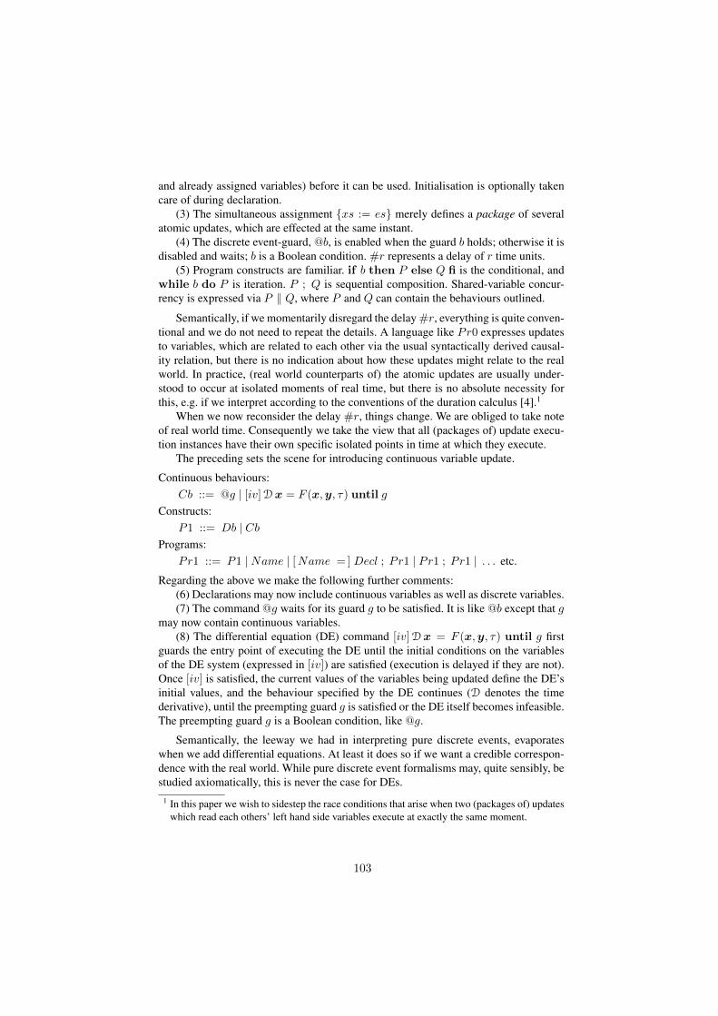
and already assigned variables) before it can be used. Initialisation is optionally takencare of during declaration.
(3) The simultaneous assignment {xs := es} merely defines a package of severalatomic updates, which are effected at the same instant.
(4) The discrete event-guard, @b, is enabled when the guard b holds; otherwise it isdisabled and waits; b is a Boolean condition. #r represents a delay of r time units.
(5) Program constructs are familiar. if b then P else Q fi is the conditional, andwhile b do P is iteration. P ; Q is sequential composition. Shared-variable concur-rency is expressed via P k Q, where P and Q can contain the behaviours outlined.
Semantically, if we momentarily disregard the delay #r, everything is quite conven-tional and we do not need to repeat the details. A language like Pr0 expresses updatesto variables, which are related to each other via the usual syntactically derived causal-ity relation, but there is no indication about how these updates might relate to the realworld. In practice, (real world counterparts of) the atomic updates are usually under-stood to occur at isolated moments of real time, but there is no absolute necessity forthis, e.g. if we interpret according to the conventions of the duration calculus [4].1
When we now reconsider the delay #r, things change. We are obliged to take noteof real world time. Consequently we take the view that all (packages of) update execu-tion instances have their own specific isolated points in time at which they execute.
The preceding sets the scene for introducing continuous variable update.
Continuous behaviours:Cb ::= @g | [iv]Dx = F (x,y, ⌧) until g
Constructs:P1 ::= Db | Cb
Programs:Pr1 ::= P1 | Name | [Name = ] Decl ; Pr1 | Pr1 ; Pr1 | . . . etc.
Regarding the above we make the following further comments:(6) Declarations may now include continuous variables as well as discrete variables.(7) The command @g waits for its guard g to be satisfied. It is like @b except that g
may now contain continuous variables.(8) The differential equation (DE) command [iv]Dx = F (x,y, ⌧) until g first
guards the entry point of executing the DE until the initial conditions on the variablesof the DE system (expressed in [iv]) are satisfied (execution is delayed if they are not).Once [iv] is satisfied, the current values of the variables being updated define the DE’sinitial values, and the behaviour specified by the DE continues (D denotes the timederivative), until the preempting guard g is satisfied or the DE itself becomes infeasible.The preempting guard g is a Boolean condition, like @g.
Semantically, the leeway we had in interpreting pure discrete events, evaporateswhen we add differential equations. At least it does so if we want a credible correspon-dence with the real world. While pure discrete event formalisms may, quite sensibly, bestudied axiomatically, this is never the case for DEs.
1 In this paper we wish to sidestep the race conditions that arise when two (packages of) updateswhich read each others’ left hand side variables execute at exactly the same moment.
103

In conventional pure and applied mathematics, the ingredients of differential equa-tions are always first interpreted with respect to a semantic domain that is stipulated inadvance (albeit often implicitly in the case of applied mathematics). Different choicesof such semantic domains are justified on grounds of the differing generality that theypermit in the properties of the functions that are deemed to solve those differential equa-tions, see e.g. [5]. Accordingly, to embed behaviours defined by differential equationsinto our language in a sound way, we must first pay some attention to matters of opera-tional semantics for the whole language. We base our treatment here on fairly standardinterpretations of state based discrete constructs and of DE systems.
Working bottom-up, the fundamental concept is the state �, a mapping from eachvariable v to a value in its type: v 7! �(v). We also need clocks, written genericallyas ⌧ . A clock is a continuous real variable whose time derivative is fixed at 1. Thephrase ‘a clock is started’ means that a fresh clock, initialised to 0, starts to run fromthe beginning of the semantic interpretation of some non-atomic construct of interest.
The Db part of the language is unsurprising. The discrete atomic variable assign-ment, x := e, sends the state � to �[�(e)/x], which is identical to �, except at x, whichbecomes �(e). Similarly for packaged atomic updates.
For @b, if b is true in the current state, then the program completes successfully.Otherwise a clock is started, and runs as long as it takes for the environment to make btrue, at which point the program completes.
For #r, if r 0, then the program completes successfully. Otherwise a clock isstarted, and runs for r > 0 time units, at which point the program completes.
For the continuous behaviours, for @g, since g may contain continuous variables,the true-set of g must be closed. With this proviso, if g is true in the current state, thenthe program completes successfully. Otherwise a clock is started, and runs as long as ittakes for the environment to make g true, at which point the program completes.
For the DE forms, we first mention some generalities.If we write a general first order differential equation as �(v,Dv, t) = 0, where v
is some tuple of real variables, Dv is a corresponding tuple of real variables intendedto denote the derivatives of v, and � is an arbitrary real-valued function, then nothingcan be said about whether any sensible interpretation of such an equation exists. Seee.g. [5], or any other rigorous text on DEs, for a wealth of counterexamples that bearthis out. Accordingly, rigorous results on differential equations that cover a reasonablywide spectrum of cases, are confined to DE forms that fit a restricted syntactic shapeand satisfy specific semantic properties. The best known such class covers first orderfamilies that can be written in the form:
Dx = F (x, ⌧) or Dx = F (x,y, ⌧)
Here, the left hand form refers to a closed system of variables x, whereas the right handform also permits the presence of additional external controls y. As well this syntacticshape, conditions have to be demanded on the vector of funtions F and on the entryconditions of the behaviour to be defined by these definitions.
For simplicity, we assume that the vector of functions F is defined on a closedrectangular region, where for each x component index i we have a Cartesian componentxi 2 [xiL . . . xiU ], and for each y component index j we have a Cartesian component
104
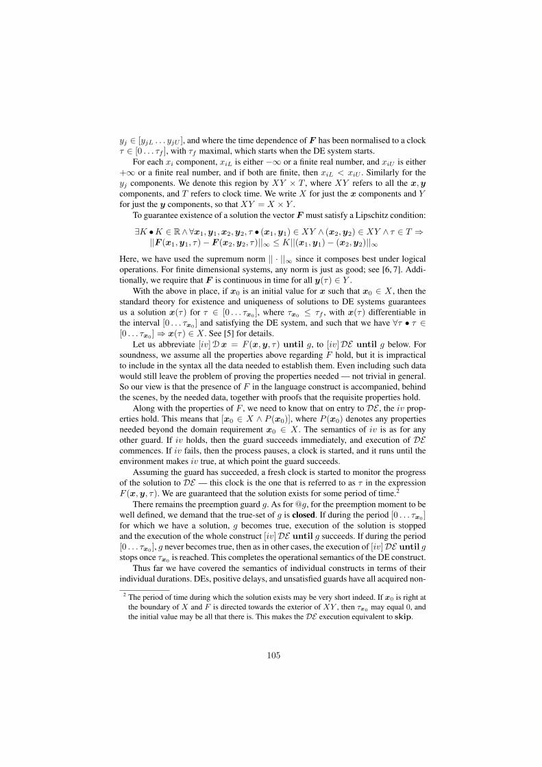
yj 2 [yjL . . . yjU ], and where the time dependence of F has been normalised to a clock⌧ 2 [0 . . . ⌧f ], with ⌧f maximal, which starts when the DE system starts.
For each xi component, xiL is either �1 or a finite real number, and xiU is either+1 or a finite real number, and if both are finite, then xiL < xiU . Similarly for theyj components. We denote this region by XY ⇥ T , where XY refers to all the x,ycomponents, and T refers to clock time. We write X for just the x components and Yfor just the y components, so that XY = X ⇥ Y .
To guarantee existence of a solution the vector F must satisfy a Lipschitz condition:
9K • K 2 R^8x1,y1,x2,y2, ⌧ • (x1,y1) 2 XY ^ (x2,y2) 2 XY ^ ⌧ 2 T )||F (x1,y1, ⌧) � F (x2,y2, ⌧)||1 K||(x1,y1) � (x2,y2)||1
Here, we have used the supremum norm || · ||1 since it composes best under logicaloperations. For finite dimensional systems, any norm is just as good; see [6, 7]. Addi-tionally, we require that F is continuous in time for all y(⌧) 2 Y .
With the above in place, if x0 is an initial value for x such that x0 2 X , then thestandard theory for existence and uniqueness of solutions to DE systems guaranteesus a solution x(⌧) for ⌧ 2 [0 . . . ⌧x0 ], where ⌧x0 ⌧f , with x(⌧) differentiable inthe interval [0 . . . ⌧x0 ] and satisfying the DE system, and such that we have 8⌧ • ⌧ 2[0 . . . ⌧x0
] ) x(⌧) 2 X . See [5] for details.Let us abbreviate [iv]Dx = F (x,y, ⌧) until g, to [iv]DE until g below. For
soundness, we assume all the properties above regarding F hold, but it is impracticalto include in the syntax all the data needed to establish them. Even including such datawould still leave the problem of proving the properties needed — not trivial in general.So our view is that the presence of F in the language construct is accompanied, behindthe scenes, by the needed data, together with proofs that the requisite properties hold.
Along with the properties of F , we need to know that on entry to DE , the iv prop-erties hold. This means that [x0 2 X ^ P (x0)], where P (x0) denotes any propertiesneeded beyond the domain requirement x0 2 X . The semantics of iv is as for anyother guard. If iv holds, then the guard succeeds immediately, and execution of DEcommences. If iv fails, then the process pauses, a clock is started, and it runs until theenvironment makes iv true, at which point the guard succeeds.
Assuming the guard has succeeded, a fresh clock is started to monitor the progressof the solution to DE — this clock is the one that is referred to as ⌧ in the expressionF (x,y, ⌧). We are guaranteed that the solution exists for some period of time.2
There remains the preemption guard g. As for @g, for the preemption moment to bewell defined, we demand that the true-set of g is closed. If during the period [0 . . . ⌧x0 ]for which we have a solution, g becomes true, execution of the solution is stoppedand the execution of the whole construct [iv]DE until g succeeds. If during the period[0 . . . ⌧x0
], g never becomes true, then as in other cases, the execution of [iv]DE until gstops once ⌧x0
is reached. This completes the operational semantics of the DE construct.Thus far we have covered the semantics of individual constructs in terms of their
individual durations. DEs, positive delays, and unsatisfied guards have all acquired non-
2 The period of time during which the solution exists may be very short indeed. If x0 is right atthe boundary of X and F is directed towards the exterior of XY , then ⌧x0 may equal 0, andthe initial value may be all that there is. This makes the DE execution equivalent to skip.
105
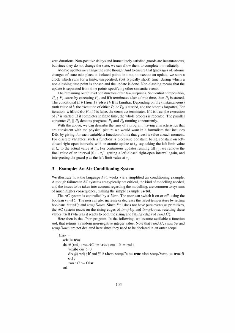
zero durations. Non-positive delays and immediately satisfied guards are instantaneous,but since they do not change the state, we can allow them to complete immediately.
Atomic updates do change the state though. And to ensure that (packages of) atomicchanges of state take place at isolated points in time, to execute an update, we start aclock which runs for a finite, unspecified, (but typically short) time, during which anon-clashing time point is chosen and the update is done. Non-clashing means that theupdate is separated from time points specifying other semantic events.
The remaining outer level constructors offer few surprises. Sequential composition,P1 ; P2, starts by executing P1, and if it terminates after a finite time, then P2 is started.The conditional if b then P1 else P2 fi is familiar. Depending on the (instantaneous)truth value of b, the execution of either P1 or P2 is started, and the other is forgotten. Foriteration, while b do P , if b is false, the construct terminates. If b is true, the executionof P is started. If it completes in finite time, the whole process is repeated. The parallelconstruct P1 k P2 denotes programs P1 and P2 running concurrently.
With the above, we can describe the runs of a program, having characteristics thatare consistent with the physical picture we would want in a formalism that includesDEs, by giving, for each variable, a function of time that gives its value at each moment.For discrete variables, such a function is piecewise constant, being constant on left-closed right-open intervals, with an atomic update at t↵ say, taking the left-limit valueat t↵ to the actual value at t↵. For continuous updates running till ⌧g , we remove thefinal value of an interval [0 . . . ⌧g], getting a left-closed right-open interval again, andinterpreting the guard g as the left-limit value at ⌧g .
3 Example: An Air Conditioning System
We illustrate how the language Pr1 works via a simplified air conditioning example.Although failures in AC systems are typically not critical, the kind of modelling needed,and the issues to be taken into account regarding the modelling, are common to systemsof much higher consequence, making the simple example useful.
The AC system is controlled by a User . The user can switch it on or off, using theboolean runAC . The user can also increase or decrease the target temperature by settingbooleans tempUp and tempDown . Since Pr1 does not have pure events as primitives,the AC system reacts on the rising edges of tempUp and tempDown , resetting thesevalues itself (whereas it reacts to both the rising and falling edges of runAC ).
Here then is the User program. In the following, we assume available a functionrnd, that returns a random non-negative integer value. Note that runAC , tempUp andtempDown are not declared here since they need to be declared in an outer scope.
User =while truedo #(rnd) ; runAC := true ; cnt : N = rnd ;
while cnt > 0do #(rnd) ; if rnd % 2 then tempUp := true else tempDown := true fiod ;runAC := false
od
106
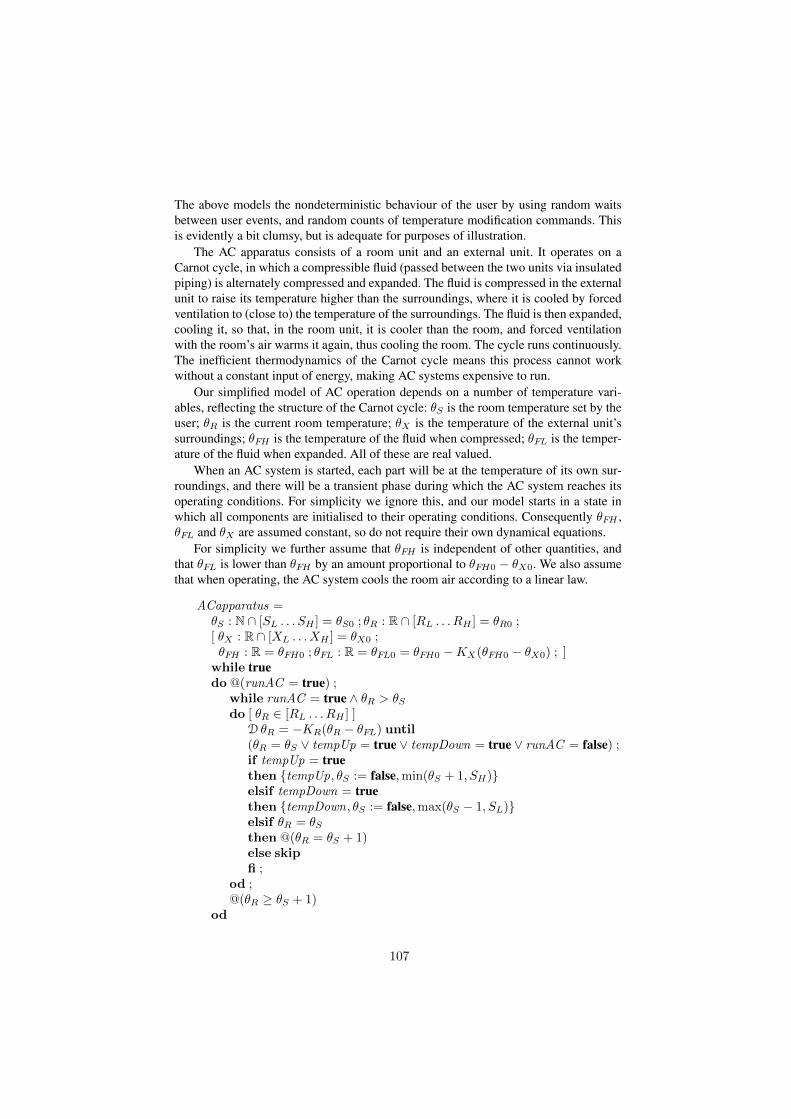
The above models the nondeterministic behaviour of the user by using random waitsbetween user events, and random counts of temperature modification commands. Thisis evidently a bit clumsy, but is adequate for purposes of illustration.
The AC apparatus consists of a room unit and an external unit. It operates on aCarnot cycle, in which a compressible fluid (passed between the two units via insulatedpiping) is alternately compressed and expanded. The fluid is compressed in the externalunit to raise its temperature higher than the surroundings, where it is cooled by forcedventilation to (close to) the temperature of the surroundings. The fluid is then expanded,cooling it, so that, in the room unit, it is cooler than the room, and forced ventilationwith the room’s air warms it again, thus cooling the room. The cycle runs continuously.The inefficient thermodynamics of the Carnot cycle means this process cannot workwithout a constant input of energy, making AC systems expensive to run.
Our simplified model of AC operation depends on a number of temperature vari-ables, reflecting the structure of the Carnot cycle: ✓S is the room temperature set by theuser; ✓R is the current room temperature; ✓X is the temperature of the external unit’ssurroundings; ✓FH is the temperature of the fluid when compressed; ✓FL is the temper-ature of the fluid when expanded. All of these are real valued.
When an AC system is started, each part will be at the temperature of its own sur-roundings, and there will be a transient phase during which the AC system reaches itsoperating conditions. For simplicity we ignore this, and our model starts in a state inwhich all components are initialised to their operating conditions. Consequently ✓FH ,✓FL and ✓X are assumed constant, so do not require their own dynamical equations.
For simplicity we further assume that ✓FH is independent of other quantities, andthat ✓FL is lower than ✓FH by an amount proportional to ✓FH0 � ✓X0. We also assumethat when operating, the AC system cools the room air according to a linear law.
ACapparatus =✓S : N \ [SL . . . SH ] = ✓S0 ; ✓R : R \ [RL . . . RH ] = ✓R0 ;[ ✓X : R \ [XL . . . XH ] = ✓X0 ;✓FH : R = ✓FH0 ; ✓FL : R = ✓FL0 = ✓FH0 � KX(✓FH0 � ✓X0) ; ]
while truedo @(runAC = true) ;
while runAC = true ^ ✓R > ✓S
do [ ✓R 2 [RL . . . RH ] ]D ✓R = �KR(✓R � ✓FL) until(✓R = ✓S _ tempUp = true _ tempDown = true _ runAC = false) ;if tempUp = truethen {tempUp, ✓S := false,min(✓S + 1, SH)}elsif tempDown = truethen {tempDown, ✓S := false,max(✓S � 1, SL)}elsif ✓R = ✓S
then @(✓R = ✓S + 1)else skipfi ;
od ;@(✓R � ✓S + 1)
od
107

Putting User and ACapparatus together gives us the complete system.
ACsystem =runAC : B = false ; tempUp : B = false ; tempDown : B = false ;(User || ACapparatus)
Note that in the above, while runAC works as a toggle, tempUp and tempDown are resetby the apparatus. Finally, we recognise that for a sensibly behaved system, we wouldneed a considerable number of relations to hold between all the constants that implicitlydefine the static structure of the system.
4 Healthiness Considerations
At this point we step back from the detailed discussion of the example to cover a num-ber of general considerations that arise when physical systems interact with computingformalisms.
[1] Allowing all variables of interest to be considered as functions of time yields aconvenient uniformity between isolated discrete updates and continuous updates. Treat-ing the two kinds in different ways can lead to a certain amount of technical awkward-ness, at the very least.
[2] When variables are functions of time, values at individual points in time haveno physical significance. Only values aggregated over an interval of time make sensephysically, and for these to be well defined, the functions of time in question have to bewell behaved enough (e.g. ‘continuous’, although ‘integrable’ would actually suffice).
[3] In dealing with CPS systems we must take into account the consequences ofusing differential equations. In a sense we have already fallen into covering this quiteextensively in discussing the semantics of our prototypical language in Section 2. Theexistence of solutions to arbitrary DEs cannot be taken for granted without the imposi-tion of appropriate sufficient conditions. An easy way to ensure this is to impose strictsyntactic restrictions on the permitted DEs, e.g. by insisting that they are linear.
[4] Physics is relentlessly eager. In conventional discrete system formalisms, as-suming that the discrete events in question are intended to correspond with real worldevents, the precise details of the correspondence with moments of time is seldom crit-ical (other than for explicitly timed systems), and more than one interpretation is per-missible, provided the causal order of events remains the same. As soon as physicalbehaviour enters the scene though, this choice disappears. If one physical behaviourstops, another must take over immediately, as the universe does not ‘go on hold’ untilsome new favourable state of affairs arises.
[5] Point [4] places quite strong restrictions on the semantics of languages intendedfor the integrated descriptions of computing and physical behaviour, since many of theoptions available for discrete systems simply disappear. Although it is perfectly possibleto design languages that ignore this consideration and integrate continuous behaviourand discrete behaviour in an arbitrary fashion, even though they may be perfectly con-sistent mathematically, unless they take due consideration of the requirements of thephysical world, they are irrelevant for the description of real world systems.
108
[6] Points [4] and [5] boil down to a requirement that decriptions of physical be-haviour must be guaranteed to be total over time. Languages intended for CPS andcritical systems should not permit gaps in time during which the behaviour of somephysical component is undefined.
[7] The requirements of the last few points can be addressed by having separateformalisms for the discrete and continuous behaviours of the whole system and havinga well thought out framework for their interworking. However, in cases of multiplecooperating formalisms, it is always the cracks between the formalisms that make themost hospitable hiding places for bugs, so particular vigilance is needed to prevent that.
[8] The impact of the preceding points may be partly addressed by careful syntacticdesign — we demonstrate this to a degree in Section 5. However, most aspects are firmlyrooted in the semantics. In this regard, a language framework that puts such semanticcriteria to the fore is highly beneficial. The semantic character of most of the issuesdiscussed implies that an approach restricted to syntactic aspects can only achieve avery limited amount.
[9] The implications of the heavily semantic nature of most of the issues discussedabove further implies the necessity of having runtime abortion as an ingredient of theoperational semantics of any language suitable for the purposes we contemplate. Al-though this is seldom an issue per se for practical languages, which must include fa-cilities for division, hence for division by zero at runtime, it is nevertheless perfectlypossible to contemplate languages in which all primitive expression building opera-tions are total, and hence to dispense with runtime abortion, even if such languages areof largely theoretical interest.
The overwhelmingly semantic nature of the preceding discussion motivates our re-ferring to the matters raised as ‘healthiness conditions’. (The nomenclature is borrowedfrom UTP [3], where appropriate structural conditions that play a similar role are bap-tised thus.) Checking that the necessary conditions hold for a given system, compelschecking that the relevant criteria, formulated as suits the language in question, holdfor the system at runtime (for the entire duration of the execution). Depending on thelanguage and how it is structured, this may turn out to be more convenient or less con-venient.
5 An Improved Concurrent Language
Taking on board the discussion in Section 4, we redesign our language as follows.
Decl ::= [x : T [ = x0 ] ; ]⇤
Db ::= x := e | {xs := es} | @b | #r
Pr0 ::= Db | Decl ; Pr0 | Pr0 ; Pr0| if b then Pr0 else Pr0 fi| while b do Pr0 od | Pr0 k Pr0
CbE ::= [iv]Dx = F (x,y, ⌧) until g | obey Rstr until g
Pr2 ::= CbE | Pr2 ; Pr2| if b then Pr2 else Pr2 fi| while b do Pr2 od | Pr2 k Pr2
PrSys ::= Name | [Name = ] Decl ; PrSys | Pr0 | Pr2 | PrSys k PrSys
109

In the above grammar, the healthiness considerations that can be addressed via the syn-tax have been incorporated. Thus, there is a visible separation between the previousdiscrete program design Pr0 (which remains unchanged), and the provisions made fordescribing physical behaviour Pr2, which have been restructured.
Specifically, there are now no facilities for Pr2 processes to wait. Furthermore,they can only be combined with discrete processes at top level, precluding their suddenappearance part way through a system run. This also means that they must be declaredat top level, reflected in the design of the PrSys syntax.
Note the additional obey clause for physical behaviour. This permits relativelyloosely defined behaviour to be specified in cases where more prescriptive behavour viaa DE is not desired or is impossible due to lack of knowledge, etc. This replaces useof waiting clauses in the earlier grammar. Note that DE behaviour and obey behaviourare the only permitted ways of describing continuous behaviour at the bottom level.
Although we have ensured that Pr2 processes cannot wait for syntactic reasons, wehave to ensure that they can’t wait for semantic reasons either. Thus we must stipulatewhat happens in the DE and obey cases when one or other of their syntactic compo-nents fails. Taking the DE case first, if iv does not evaluate to true,3 then the wholetop level PrSys process must abort, that is to say, execution terminates abruptly in afailing state. If F fails to satisfy the conditions for existence of a DE solution, thenthe top level PrSys process aborts. If g does not evaluate to true at some moment inthe DE solution, in case that the duration of the DE solution ⌧f is finite, then when⌧f is reached, the top level PrSys process aborts. Turning to the obey case, if Rstrdoes not evaluate to true in a left closed right open time interval starting from the mo-ment the obey construct is encountered (or amounts to skip at that moment), then toplevel PrSys process aborts. If g does not evaluate to true at some moment during thetrue interval of Rstr, in case that the duration of the true interval of Rstr, say ⌧f , isfinite, then when ⌧f is reached, the top level PrSys process aborts.
Having defined the improved language, we can check over how it addresses thehealthiness conditions described earlier. Re. [1], we have already stipulated that allvariables depend on time in our description of the semantics, so [1] is covered. Re. [2],this is again implicit in our semantics. Likewise, [3] is also covered by our relativelydetailed discussion of DEs. Re. [4], we have designed the syntax to prohibit explicitlazy behaviour in the continuous domain, and this is backed up by the semantics whichdisallows lazy behaviour arising from runtime conditions — this justification extends topoint [5], and this, combined with the fact that DE behaviour and obey behaviour arethe only permitted ways of describing continuous behaviour at the bottom level guar-antee totality over time provided the behaviour described by the syntax is well definedsemantically, covering point [6]. Points [7] and [8] are things that can be achieved syn-tactically, and our design does so. Point [9] indicates the necessity of having runtimeaborts in the semantics, this being forced by the eagerness of physical behaviour. Theneed for this also arose in our remarks regarding point [6].
The heavy dependence on semantics of this discussion raises the question of howwe can be sure that any system that is written down defines a sensible behaviour. In
3 That is to say, it evaluates to false, or fails to evaluate at all.
110
purely discrete languages, there is a well trodden route from the syntactic structure of asystem description to verification conditions that confirm the absence of runtime errors.
The same approach extends to languages containing continuous update, such asours. The syntactic structure of such a language can be analysed to elicit all the de-pendencies between different syntactic elements that can arise at runtime, and thesedependencies can be used to create template verification conditions. Given a specificmodel, the generic template verification conditions can be instantiated to the elementsof the model to provide sufficient (although not necessarily necessary) conditions forruntime well definedness. Still, it has to be conceded that such conditions can be morechallenging than in the discrete case because of the more subtle nature of aspects ofcontinuous mathematics.
Although we do not give a comprehensive account of the verification templatesfor our (improved) language (it has, after all, been constructed just for illustrative pur-poses), we can give an indication of a couple of them.
Thus, if the flow of control reaches an DE construct [iv]Dx = F (x,y, ⌧) until gwe need to know the initial value guard will succeed. We can ensure statically that thiswill be the case if the DE construct occurs in a case analysis whose collection of guardscovers all values that could be generated.
Similarly, once a DE construct has been preempted by its preemption guard becom-ing true, we need to ensure that there is a viable continuous successor behaviour forthe physical process to engage in. This is helped in our case by the syntax, and can besupported by a proof that the truth of the preemption guard enables some syntacticallyavailable successor option.
In the discrete part of the language, the success of an if statement can be assuredprovided there is a default else clause to capture any exceptional cases. And so on.
Still, achieving full static assurance of freedom from runtime errors may requirefully simulating the system, which will usually be impractical. Much depends on thelanguage design. To help the process, languages may be designed in which all expres-sion forming constructs are guaranteed to denote (e.g. in extremis by not having divisionin the language). Such languages may help in the verified design of critical systems.
6 The Running Example, Improved
In the light of the preceding discussions, we return to our running example and restruc-ture it for the improved language. For simplicity we will omit the bracketed constantdeclarations that appeared in the earlier ACapparatus. We also keep the definition ofthe User the same, as that conforms to the syntax of the improved language. Regardingthe ACapparatus, it requires some significant restructuring.
Firstly, the previous design mixed discrete and continuous update in a fairly uncrit-ical manner. Thus the DE D ✓R = �KR(✓R � ✓FL), describing the fluid behaviour,is mixed with discrete updates to ✓S , done at the behest of the User. Worse, when theDE is preempted, no physical behaviour is defined for the fluid — the ACapparatus justhangs around waiting for the next opportunity to do some cooling. This is not really ac-ceptable: the fluid does not stop being a physical system, subject to the laws of nature,
111
just because, with our focus on the ACapparatus design, we have no great interest in itsbehaviour during a particular period.
Our restructured design separates the physical from the discrete aspects. The earlierACapparatus is split into an ACcontroller process, looking after the discrete updates,and a ACfluid process, which describes the physical behaviour of the fluid.
Normally, the User would communicate with the ACcontroller, which would thencontrol the ACfluid, but we are a bit sloppy, and allow the User’s runAC variable toalso directly control the ACfluid, thus sharing the fluid control between the User andthe ACcontroller. The latter therefore just controls the ✓S value while runAC is true.
The ACfluid process, now constrained by the restricted syntax for physical pro-cesses, describes the fluid’s properties at all times. At times when the DE behaviouris not relevant, an obey clause defines default behaviour, amounting to ✓R remainingwithin the expected range. The separation of control and fluid allows us to make thefluid responsible for detecting temperature and to only initiate the DE behaviour whenthe temperature is at least a degree above the set point ✓S . Of course this is rather un-realistic, and a more credible (and detailed) design would involve sensors under thecontrol of the ACcontroller to manage this aspect.
ACcontroller =while truedo @(runAC = true) ;
while runAC = true ^ ✓R > ✓S
do @(tempUp = true _ tempDown = true _ runAC = false) ;if tempUp = truethen {tempUp, ✓S := false,min(✓S + 1, SH)}elsif tempDown = truethen {tempDown, ✓S := false,max(✓S � 1, SL)}fi
odod
ACfluid =while truedo obey ✓R 2 [RL . . . RH ] until runAC = true ;
if ✓R � ✓S + 1then [ ✓R 2 [RL . . . RH ] ] D ✓R = �KR(✓R � ✓FL)
until (✓R = ✓S _ runAC = false)else obey ✓R 2 [RL . . . RH ] until ✓R � ✓S + 1 _ runAC = falsefi
od
Putting all three components together gives us the complete system.
ACsystem =runAC : B = false ; tempUp : B = false ; tempDown : B = false ;(User || ( ✓S : N \ [SL . . . SH ] = ✓S0 ; ✓R : R \ [RL . . . RH ] = ✓R0 ;
ACcontroller || ACfluid ) )
112
7 Related Approaches
It is fair to say that the critical systems industry is rather conservative — advocatingradical new ways of doing things that do not enjoy the highest levels of trust risks majordisasters in the field. Even the newer standards in key fields, such as DO-178C (foravionics [8]), ISO 26262 (for automotive systems [9]), IEC 62304 (for medical devices[10]), or CENELEC EN 50128 (for railway systems [11]), are still heavily weightedin favour of mandating specific testing strategies, and other practices heavily rootedin traditional development techniques. Thus the entry of formal techniques into thestandardised critical systems development portfolio is rather cautious, despite the strongevidence in niche quarters about the dependability that can be gained by appropriate useof formal development, suitably integrated into the wider system engineering process.This is as much because entrenched industrial practice cannot move as nimbly as onemight hope, even when the evidence for attempting to do so is relatively strong.
Here, we briefly comment on some approaches that compare with our exercise torealign a candidate language for utility in the cyberphysical and critical systems arena.
In the cyberphysical systems area [12–14], we can point to the extensive survey [15],which covers a wide spectrum of research into cyberphysical systems, and the toolsand techniques used in that sphere. As we might expect, despite the relative newnessof the cyberphysical systems area, formal approaches are somewhat overshadowed bymore traditional and simulation based techniques. Again, this is due to the fact thatcyberphysical systems still have to be built, and this falls back on traditional approaches.
The older survey [16] is more linguistically based and covers a large spectrum oflanguages and tools for hybrid systems. One is struck by the typically low expressivityin the continuous sphere of many of the systems discussed there, motivated, of course,by the desire for decidability of the resulting languages and systems. For decidabilityreasons, most of these are based on variations of the hybrid automaton concept [17–19].In fact, for simple linear behaviours, e.g. Dx = K, with K constant, there is very littledifference between using a DE as just quoted, and using an expression x0 = x + K�Twhere �T is the duration of the behaviour.
Neverthless, many of the formalisms in these sources are focused on the single goalof hybrid or continuous behaviour, to the exclusion of more general computing con-cerns. This leads to the ‘bugs in between formalisms’ risk noted earlier, when multipleformalisms need to be combined.
Closer to our perspective is the work of Platzer [20], supported by the KeyMaeratool [21]. This supports the kind of modelling exemplified in this paper, with a strongfocus on verification. Alternatively there is the Hybrid Event-B formalism [22, 23]. Thisis an extension of the pure discrete event formalism Event-B [24], building on the earlierclassical B-Method [25], (which is still actively used in critical applications in the urbanrail sector [26]). The extension is expressly designed to avoid the kind of traps regardingcontinuous behaviour and verification that we illustrated earlier in this paper.
Thus far our discussion has avoided mentioning noise or randomness. This is le-gitimate when the physical considerations imply that it is negligible. But if sourcesof uncertainty are significant, then probabilistic techniques need to be taken on board.These add nontrivial complication to the semantics of any language. An indication ofthe issues that can arise can be found in [27, 28].
113
8 Conclusion
Motivated by the current dramatic proliferation in critical and cyberphysical systems,especially in urbanised areas all over the world, in the preceding sections, we exam-ined the problem of extending typical existing, more conventional formalisms for pro-gramming, to allow them to incorporate the needed physical behaviour that is a vitalingredient of these systems. Such integrated formalisms can come into their own ifwe contemplate the integrated verification of critical cyberphysical systems, in whichwe seek to avoid the possibilities of there being bugs that hide in the semantic cracksbetween separate formalisms that are used to check separate parts of the behaviour.
Rather than being comprehensive, our approach in this paper has been to illustratethe range of issues to be considered, by taking a somewhat prototypical shared variablelanguage for concurrent sequential programming, and extending it in a relatively naıveway to incorporate continuous behaviour. We then critically examined the consequencesof this, and identified a number of issues that are not always taken sufficient account ofwhen embarking on such an extension exercise. For want of a pithy name, we termedthese ‘healthiness considerations’, by analogy with the nomenclature used in UTP. Thisdone, we showed how the earlier naıve syntax could be improved to partially addresssome of these issues, the remainder being the responsibility of the semantics.
We illustrated our particular solution with a simplified air conditioning system, giv-ing the core steady state behaviour in both the original and improved formulations.
It is important to emphasise that we do not claim that the details of our solution(even in the case of our specific language) are unique. One could resolve the sameissues in a number of ways that differed in the low level detail. Nevertheless, the broadsweep of the things needing to be considered would remain similar.
We also do not claim that our language (and its improved version) are to be partic-ularly recommended for critical cyberphysical system development. In many ways, theissues we have striven to highlight are brought our more clearly in a language whichone would rather not choose to use.
We can liken the urge to match the surface syntactic features of the language asclosely as possible to what is needed by the semantics of the physical considerations,with the longstanding process whereby machine code was superseded by assembly lan-guage, which was superseded by higher level languages, etc., in each case the desirebeing to raise the level of abstraction in such a way as to preclude as many user level er-rors as possible by making them syntactically illegal (or simply impossible to express),and backing this up semantically.
It is to be hoped that the insights from an exercise like the one we have undertakencan help to improve the broader awareness of the issues lurking under the bonnet whenformalisms for critical and cyberphysical systems are designed in future.
References
1. Alur, R.: Principles of Cyberphysical Systems. MIT Press (2015)2. Lee, E., Shesha, S.: Introduction to Embedded Systems: A Cyberphysical Systems Ap-
proach. 2nd. edn. LeeShesha.org (2015)
114
3. Hoare, T., , He, J.: Unifying Theories of Programming. Prentice-Hall (1998)4. Zhou, C., Hoare, T., Ravn, A.: A Calculus of Durations. Inf. Proc. Lett. 40 (1991) 269–2765. Walter, W.: Ordinary Differential Equations. Springer (1998)6. Horn, R., Johnson, C.: Matrix Analysis. Cambridge University Press (1985)7. Horn, R., Johnson, C.: Topics in Matrix Analysis. Cambridge University Press (1991)8. DO-178C: http://www.rtca.org.9. ISO 26262: http://www.iso.org/iso/home/store/catalogue_tc/
catalogue_detail.htm?csn%umber=54591.10. IEC 62304: https://webstore.iec.ch/preview/info_iec62304{ed1.
0}en_d.pdf.11. CENELEC EN 50128: https://www.cenelec.eu/dyn/www/f?p=104:105.12. Sztipanovits, J.: Model Integration and Cyber Physical Systems: A Semantics Perspec-
tive. In Butler, Schulte, eds.: Proc. FM-11, Springer, LNCS 6664, p.1, http://sites.lero.ie/download.aspx?f=Sztipanovits-Keynote.pdf (2011) Invited talk,FM 2011, Limerick, Ireland.
13. Willems, J.: Open Dynamical Systems: Their Aims and their Origins. Ru-berti Lecture, Rome (2007) http://homes.esat.kuleuven.be/˜jwillems/Lectures/2007/Rubertilecture.pd%f.
14. National Science and Technology Council: Trustworthy Cyberspace: Strategic plan for theFederal Cybersecurity Research and Development Program (2011)http://www.whitehouse.gov/sites/default/files/microsites/ostp/fed_cyber%security_rd_strategic_plan_2011.pdf.
15. Geisberger, E., Broy (eds.), M.: Living in a Networked World. Integrated Re-search Agenda Cyber-Physical Systems (agendaCPS) (2015) http://www.acatech.de/fileadmin/user_upload/Baumstruktur_nach_Website/A%catech/root/de/Publikationen/Projektberichte/acaetch_STUDIE_agendaCPS_eng_WEB.%pdf.
16. Carloni, L., Passerone, R., Pinto, A., Sangiovanni-Vincentelli, A.: Languages and Tools forHybrid Systems Design. Foundations and Trends in Electronic Design Automation 1 (2006)1–193
17. Henzinger, T.: The Theory of Hybrid Automata. In: Proc. IEEE LICS-96, IEEE (1996)278–292 Also http://mtc.epfl.ch/˜tah/Publications/the_theory_of_hybrid_automata.pdf.
18. Alur, R., Courcoubetis, C., Henzinger, T., Ho, P.H.: Hybrid Automata: An AlgorithmicApproach to the Specification and Verification of Hybrid Systems. In: Proc. Workshop onTheory of Hybrid Systems. Volume 736 of LNCS., Springer (1993) 209–229
19. Alur, R., Dill, D.: A Theory of Timed Automata. Theor. Comp. Sci. 126 (1994) 183–23520. Platzer, A.: Logical Analysis of Hybrid Systems: Proving Theorems for Complex Dynamics.
Springer (2010)21. Symbolaris: http://www.symbolaris.org.22. Banach, R., Butler, M., Qin, S., Verma, N., Zhu, H.: Core Hybrid Event-B I: Single Hybrid
Event-B Machines. Sci. Comp. Prog. 105 (2015) 92–12323. Banach, R., Butler, M., Qin, S., Zhu, H.: Core Hybrid Event-B II: Multiple Cooperating
Hybrid Event-B Machines. (2015) Submitted.24. Abrial, J.R.: Modeling in Event-B: System and Software Engineering. Cambridge University
Press (2010)25. Abrial, J.R.: The B-Book: Assigning Programs to Meanings. Cambridge University Press
(1996)26. Clearsy: http://www.clearsy.com/en/.27. Zhu, H., Qin, S., He, J., Bowen, J.: PTSC: Probability, Time and Shared-Variable Concur-
rency. Innov. Syst. Softw. Eng. 5 (2009) 271284
115

28. Zhu, H., Yang, F., He, J., Bowen, J., Sanders, J., Qin, S.: Linking Operational Semanticsand Algebraic Semantics for a Probabilistic Timed Shared-Variable Language. J. Log. Alg.Prog. 81 (2012) 2–25
116
Applying parametric model-checking techniquesfor reusing real-time critical systems?
Baptiste Parquier1, Laurent Rioux1, Rafik Henia1, Romain Soulat1, Olivier H.Roux2, Didier Lime2, and Etienne Andre3
1 THALES Research & Technology, 1 avenue Augustin Fresnel, 91120 Palaiseau,France
2 IRCCyN, 1 rue de la Noe, 44300 Nantes, France3 Universite Paris 13, Sorbonne Paris Cite, LIPN, CNRS, UMR 7030, F-93430,
Villetaneuse, France
Abstract. Due to the increase of complexity in real-time safety-criticalsystems, verification and validation costs have significantly increased. Astraightforward way to reduce costs is to reuse existing systems, adaptingthem to new requirements, so as to avoid new costly developments. Ouraim is to verify during the development strategy definition phase whetherthe existing products can be reused and adapted for a new customer,by identifying key parameters to be tuned in order to reuse existingproducts. Performing e�cient verification is therefore crucial.In this paper, we focus on the performance requirement aspects. Nowa-days, model-checking techniques have improved significantly to verifythe performances of real-time systems. However, model-checking cannotaddress real-time systems where some timing constants are unknown oruncertain. Parametric model-checking leverage this shortcoming by iden-tifying parameter ranges for which the system is correct. We report hereon an experiment of the evaluation of the use of these formal techniquesapplied to automatize the synthesis of good parameter ranges for systemreuse in the setting of the environment requirements for an aerial videotracking system.
Keywords: real-time systems, safety-critical systems, formal methods,parametric verification, performance verification, case study, avionics
1 Introduction
Performance verification is a common discipline in system and software engi-neering. In practice, it is very common to spend a lot of e↵ort in performanceengineering especially for certified products. Standards specify a complete andprecise safety process to follow in order to be certified (e. g., DO-178C in theavionics domain). There is a need to reduce the time and e↵orts related to de-sign such real-time systems considering performance requirements. We would
? This work is partially supported by the ANR national research program ANR-14-CE28-0002 PACS (“Parametric Analyses of Concurrent Systems”).
117
2
like to experiment and verify if the current state of the art on performance ver-ification tools are able to cope with industrial needs. We will not address thewhole performance engineering process. We will focus on the performance verifi-cation in a particular context: an industrial company plans to reuse an existingreal-time safety-critical system for the needs of a new client to cut costs anddelays. However, this client is coming with its own performance requirementsthat di↵ers from what the system was originally designed for. Our use case is anaerial video tracking device. Its mission is safety-critical for the whole systemand, therefore, has to be certified according to the DO-178C standard.
To this end, we have to demonstrate the software architecture meets theperformance requirements, which implies that the system has to satisfy all thedeadline requirements in all (and in particular the worst) situations.
A conventional way at THALES – but also in other industrial companies– to tackle this problem is to evaluate the performance of the current system.The system is taken as is and if it satisfies the client performance requirements,the system can be reused as it stands. If not, experts check how to modifyenvironment parameters – typically sources of activation of the system – and tryto identify a new configuration where the system can meet its new requirements.This is time consuming and costly. Therefore, generally only few configurationsare tested and evaluated, and quite often, none of them meets the requirements.As a consequence when the activity is seen as too costly, the “reuse” strategy isdropped.
We report here on an experimentation to apply formal techniques on anaerial video tracking system by THALES, in a way to tool-up the identificationof the good environment parameters to reuse the system. Our methodology is asfollows:
1. We first identified the most appropriate formalisms and formal techniquesto validate the performance and identify the good environment parameters:we chose to use parametric stopwatch automata (PSwAs) and parametricstopwatch Petri nets (PSwPNs), two formalisms for modeling and verifyingpreemptive real-time systems with parameters. These two formalisms benefitfrom state-of-the-art model-checkers (IMITATOR for PSwAs and Romeo forPSwPNs).
2. We then devised a way to model the system needed for performance valida-tion, using the identified formalisms.
3. We then studied how to measure the trust in the results produced by IMI-
TATOR and Romeo: In this regard, we exploit diversity: the use of severaltechniques giving the very same results is a great source of confidence. Nev-ertheless, diversity can only be reached if the alternatives used are trulydi↵erent and cannot both fail due to some common weaknesses.
Organization of the paper Section 2 presents the aerial video tracking systemdeveloped by THALES, and its new requirements. Section 3 presents the stateof the art of available verification techniques, in particular formal methods usingparameterization. Section 4 introduces the tools Romeo and IMITATOR respec-tively for parametric stopwatch Petri nets and parametric stopwatch automata.
118
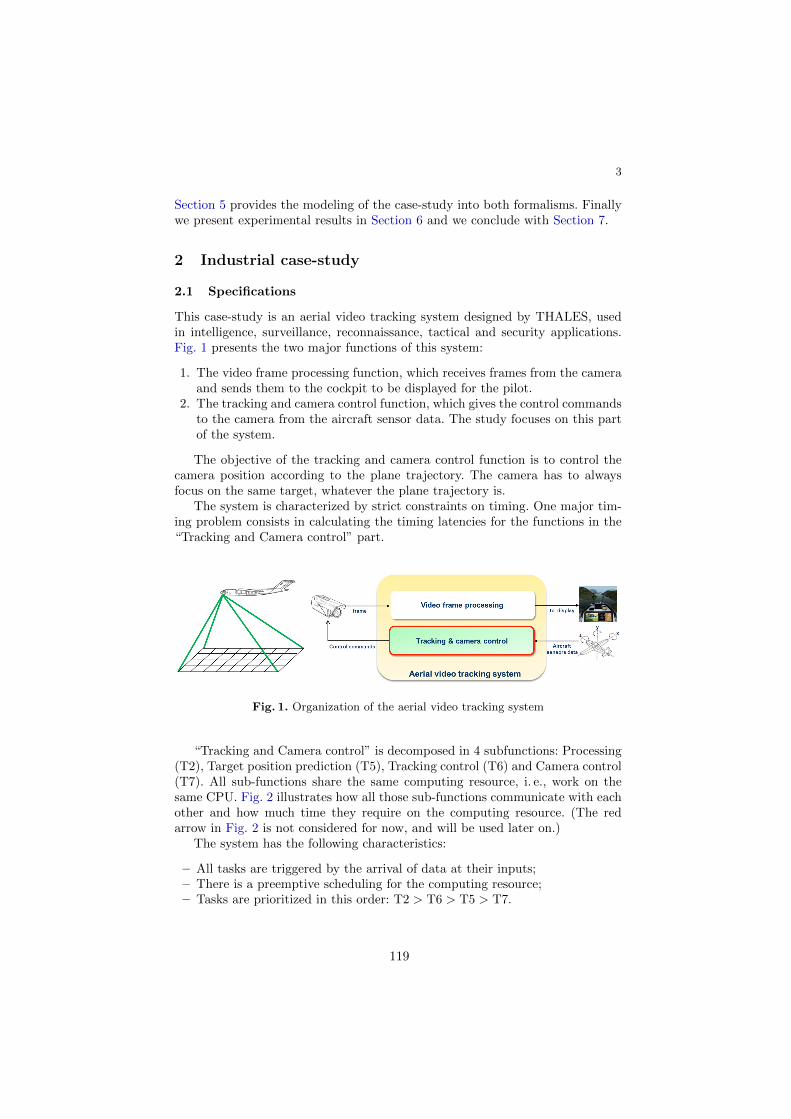
3
Section 5 provides the modeling of the case-study into both formalisms. Finallywe present experimental results in Section 6 and we conclude with Section 7.
2 Industrial case-study
2.1 Specifications
This case-study is an aerial video tracking system designed by THALES, usedin intelligence, surveillance, reconnaissance, tactical and security applications.Fig. 1 presents the two major functions of this system:
1. The video frame processing function, which receives frames from the cameraand sends them to the cockpit to be displayed for the pilot.
2. The tracking and camera control function, which gives the control commandsto the camera from the aircraft sensor data. The study focuses on this partof the system.
The objective of the tracking and camera control function is to control thecamera position according to the plane trajectory. The camera has to alwaysfocus on the same target, whatever the plane trajectory is.
The system is characterized by strict constraints on timing. One major tim-ing problem consists in calculating the timing latencies for the functions in the“Tracking and Camera control” part.
Fig. 1. Organization of the aerial video tracking system
“Tracking and Camera control” is decomposed in 4 subfunctions: Processing(T2), Target position prediction (T5), Tracking control (T6) and Camera control(T7). All sub-functions share the same computing resource, i. e., work on thesame CPU. Fig. 2 illustrates how all those sub-functions communicate with eachother and how much time they require on the computing resource. (The redarrow in Fig. 2 is not considered for now, and will be used later on.)
The system has the following characteristics:
– All tasks are triggered by the arrival of data at their inputs;– There is a preemptive scheduling for the computing resource;– Tasks are prioritized in this order: T2 > T6 > T5 > T7.
119
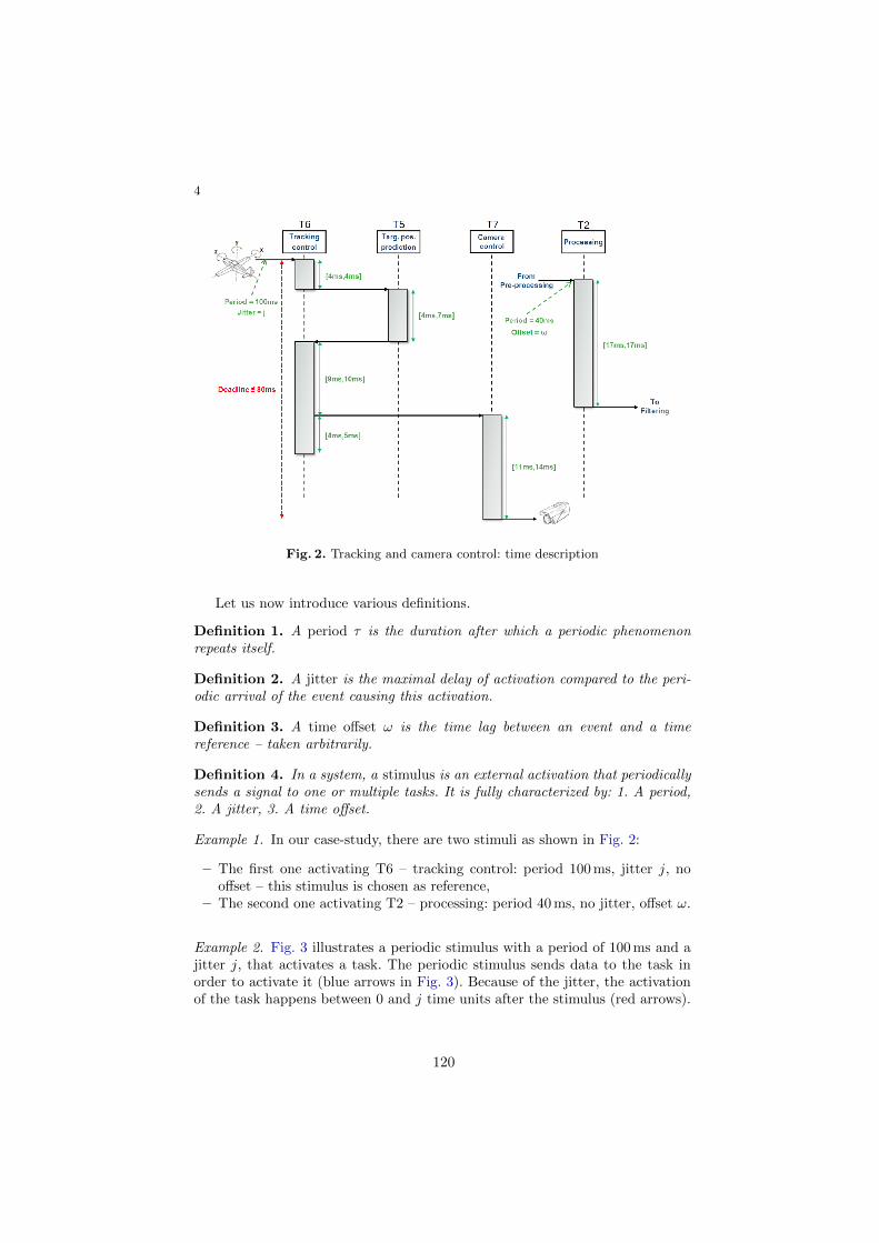
4
Fig. 2. Tracking and camera control: time description
Let us now introduce various definitions.
Definition 1. A period ⌧ is the duration after which a periodic phenomenonrepeats itself.
Definition 2. A jitter is the maximal delay of activation compared to the peri-odic arrival of the event causing this activation.
Definition 3. A time o↵set ! is the time lag between an event and a timereference – taken arbitrarily.
Definition 4. In a system, a stimulus is an external activation that periodicallysends a signal to one or multiple tasks. It is fully characterized by: 1. A period,2. A jitter, 3. A time o↵set.
Example 1. In our case-study, there are two stimuli as shown in Fig. 2:
– The first one activating T6 – tracking control: period 100ms, jitter j, noo↵set – this stimulus is chosen as reference,
– The second one activating T2 – processing: period 40 ms, no jitter, o↵set !.
Example 2. Fig. 3 illustrates a periodic stimulus with a period of 100 ms and ajitter j, that activates a task. The periodic stimulus sends data to the task inorder to activate it (blue arrows in Fig. 3). Because of the jitter, the activationof the task happens between 0 and j time units after the stimulus (red arrows).
120

5
Fig. 3. A 30 ms jitter on a 100 ms period stimulus
The jitter j represents a potential delay due to the communication network inthe aircraft. It is not something that can be determined at design time: the besta designer can do is to take into account that there will be a possible delay in thefinal system and ensure the system will behave according to the requirementswhatever the jitter is. Until now, system environment ensured that:
j = 30ms
The o↵set ! might be used to change the reference between T6’s and T2’sactivations. An o↵set is something the designer can tune to ensure the systemgood behavior.
2.2 Main objective
Our main objective is to reuse an existing system for new customers, which meansthe system has to meet all new performance requirements. More precisely, in thisexperiment, we consider the situation where a new customer wants to modifythe following requirement to the aerial video tracking system: “The end-to-endlatency between the activation of task T6 and the termination of task T7 shallbe lower than 80ms.” The new end-to-end latency requirement is depicted inred in Fig. 2.
Our aim is to compute new timing specifications of the system so that thisadditional requirement can be met. However, the heart of the system must notchange. As the system is expected to be reused as is, we can only modify thetiming specifications of external activations: tune the o↵set between stimuli, orchange the jitter requirements.
2.3 Our constraints: a parametric approach
In our case study, jitter and o↵set can be seen as parameters. Moreover, eventiming properties can be expressed parametrically, as timing constraints makesense only in the context of a given concrete environment. For example, a maxi-mal delay of the system response has to be at most two times the minimal delay,or the transmission time in the communication protocol could be left as a pa-rameter. Performing non-parametric model-checking of the systems for di↵erentconcrete values is di�cult and leads to state-space explosion. The possibility tospecify parametric timing constraints is then a great opportunity that allows toevaluate timing performances of real-time systems independently of their par-ticular implementation.
We summarize the main needs for a parametric approach:
121
6
– Parameters allow to cope with the early uncertainties in developing an in-dustrial system;
– Parameters allow to investigate robustness of some of the design choices;– If the system is proven wrong, the whole verification process has to be carried
out again;– Considering a wide range of values for constants allows for a more flexible
and robust design.
3 Related works
3.1 Response time and latency analysis
As mentioned in [21], many research papers have already addressed the problemof parametric schedulability analysis, especially on single processor systems. Biniand Buttazzo [10] proposed an analysis of fixed priority single processor systems,which is used as a basis for this paper.
Parameter sensitivity can be also be carried out by repeatedly applying clas-sical schedulability tests, like the holistic analysis [19]. One example of this ap-proach is used in the Mast tool [13], in which it is possible to compute the slack(i. e., the percentage of variation) with respect to one parameter for single pro-cessor and for distributed systems by applying binary search in that parameterspace [19].
A similar approach is followed by the SymTA/S tool [14], which is basedon the event-stream model [20]. Another interesting approach is the ModularPerformance Analysis (MPA) [23], which is based on Real-Time Calculus. Inboth cases, the analysis is compositional, therefore less complex than the holisticanalysis. In [16], a real time system is modeled using a high level variant of timedautomata including design timed parameters and is analyzed using the UPPAALtool. Nevertheless, these approaches are not fully parametric, in the sense thatit is necessary to repeat the analysis for every combination of parameter valuesin order to obtain the schedulability region.
3.2 Parametric formalisms for real-time systems
The literature proposes mainly two formalisms to model and verify systemswith timing parameters: parametric timed automata [3] and parametric timePetri nets [22]. Both formalisms are subject to strong undecidability results,even with low numbers of parameters [18], syntactic restrictions such as strictconstraints [12], or with restricted parameter domains, such as bounded ratio-nals [18], or (unbounded) integers [3] (see [5] for a survey). Undecidability isnot necessarily a problem: semi-algorithms were defined (e. g., [3,6,15]) and safeunder-approximations were also proposed (e. g., [15,8]).
For many real-time systems, in particular when subject to preemptive schedul-ing, these formalisms are not expressive enough. As a consequence, we thereforeuse extensions of parametric timed automata and parametric time Petri nets
122
7
augmented with stopwatches, yielding parametric stopwatch automata [21], andparametric stopwatch Petri nets [22].
To the best of our knowledge, the only tools using as basis formalism thesetwo formalisms are IMITATOR [7] for parametric stopwatch automata, and Romeo [17]for parametric stopwatch Petri nets. In this work, we evaluate the capabilitiesof both tools using the industrial case study.
4 Tools
We briefly present both tools in the following. Using tools is an opportunity toincrease the confidence in our results. We believe this o↵ers us the diversity weseek for in our approach, because the tools are developed by di↵erent teams,and based on di↵erent theories: parametric stopwatch Petri nets vs. parametricstopwatch automata, that implies di↵erent models.
By doing that, the confidence one can have in both tools increases consider-ably: if both tools give the same results, the odds that they are both wrong isclearly very low, and therefore the confidence is high.
4.1 Romeo
Romeo4 [17] is a software studio for parametric analysis of time Petri nets andsome of their hybrid extensions (such as parametric stopwatch Petri nets). It isavailable for Linux, MacOSX and Windows platforms and consists of a graphicaluser interface (GUI) to edit and design PSwPNs, and a computation engine.
Romeo supports the use of parametric linear expressions in the time intervalsof the transitions, and allows to add linear constraints on the parameters torestrict their domain. Finally, Romeo provides a simulator and an integratedTCTL model-checker [11].
4.2 IMITATOR
IMITATOR5 [7] is a software for parametric verification and robustness analysisof real-time systems. It relies on the formalism of networks of parametric timedautomata, augmented with integer variables and stopwatches. Parameters canbe used both in the model and in the properties.
IMITATOR is fully written in OCaml, and makes use of the Parma PolyhedraLibrary [9]. It is available under the GNU General Public License.
5 Modeling the case-study
Modeling the system in both tools was one of the challenges of this work. Eachtheory has its particularities, and translating the case-study specifications ac-cording to the associated theory was sometimes problematic. This part presents
4 http://romeo.rts-software.org5 http://www.imitator.fr
123
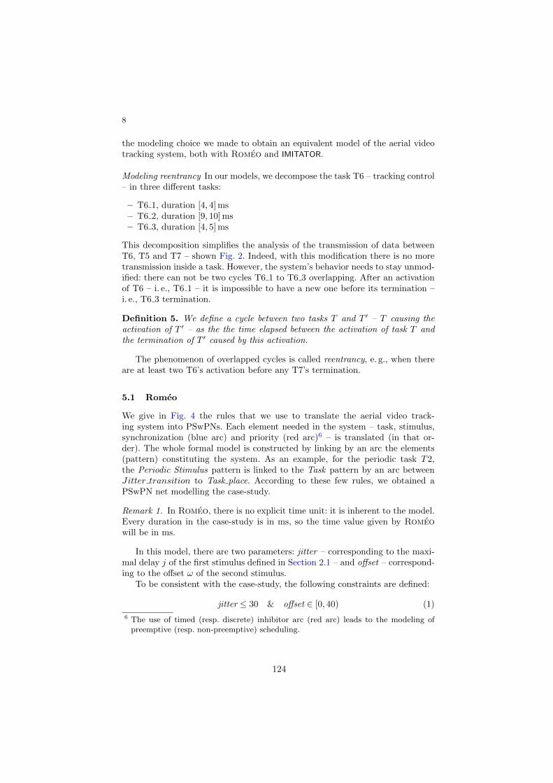
8
the modeling choice we made to obtain an equivalent model of the aerial videotracking system, both with Romeo and IMITATOR.
Modeling reentrancy In our models, we decompose the task T6 – tracking control– in three di↵erent tasks:
– T6 1, duration [4, 4] ms– T6 2, duration [9, 10] ms– T6 3, duration [4, 5] ms
This decomposition simplifies the analysis of the transmission of data betweenT6, T5 and T7 – shown Fig. 2. Indeed, with this modification there is no moretransmission inside a task. However, the system’s behavior needs to stay unmod-ified: there can not be two cycles T6 1 to T6 3 overlapping. After an activationof T6 – i. e., T6 1 – it is impossible to have a new one before its termination –i. e., T6 3 termination.
Definition 5. We define a cycle between two tasks T and T 0 – T causing theactivation of T 0 – as the the time elapsed between the activation of task T andthe termination of T 0 caused by this activation.
The phenomenon of overlapped cycles is called reentrancy, e. g., when thereare at least two T6’s activation before any T7’s termination.
5.1 Romeo
We give in Fig. 4 the rules that we use to translate the aerial video track-ing system into PSwPNs. Each element needed in the system – task, stimulus,synchronization (blue arc) and priority (red arc)6 – is translated (in that or-der). The whole formal model is constructed by linking by an arc the elements(pattern) constituting the system. As an example, for the periodic task T2,the Periodic Stimulus pattern is linked to the Task pattern by an arc betweenJitter transition to Task place. According to these few rules, we obtained aPSwPN net modelling the case-study.
Remark 1. In Romeo, there is no explicit time unit: it is inherent to the model.Every duration in the case-study is in ms, so the time value given by Romeowill be in ms.
In this model, there are two parameters: jitter – corresponding to the maxi-mal delay j of the first stimulus defined in Section 2.1 – and o↵set – correspond-ing to the o↵set ! of the second stimulus.
To be consistent with the case-study, the following constraints are defined:
jitter 30 & o↵set 2 [0, 40) (1)
6 The use of timed (resp. discrete) inhibitor arc (red arc) leads to the modeling ofpreemptive (resp. non-preemptive) scheduling.
124
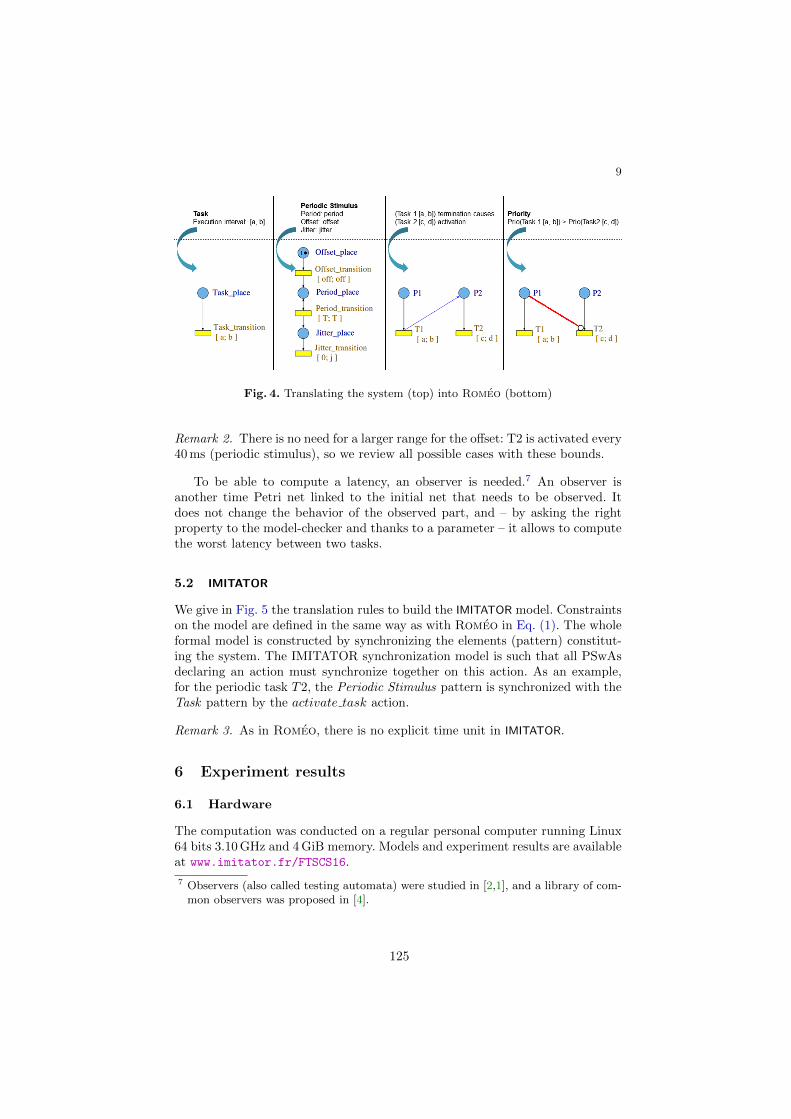
9
Fig. 4. Translating the system (top) into Romeo (bottom)
Remark 2. There is no need for a larger range for the o↵set: T2 is activated every40 ms (periodic stimulus), so we review all possible cases with these bounds.
To be able to compute a latency, an observer is needed.7 An observer isanother time Petri net linked to the initial net that needs to be observed. Itdoes not change the behavior of the observed part, and – by asking the rightproperty to the model-checker and thanks to a parameter – it allows to computethe worst latency between two tasks.
5.2 IMITATOR
We give in Fig. 5 the translation rules to build the IMITATOR model. Constraintson the model are defined in the same way as with Romeo in Eq. (1). The wholeformal model is constructed by synchronizing the elements (pattern) constitut-ing the system. The IMITATOR synchronization model is such that all PSwAsdeclaring an action must synchronize together on this action. As an example,for the periodic task T2, the Periodic Stimulus pattern is synchronized with theTask pattern by the activate task action.
Remark 3. As in Romeo, there is no explicit time unit in IMITATOR.
6 Experiment results
6.1 Hardware
The computation was conducted on a regular personal computer running Linux64 bits 3.10 GHz and 4 GiB memory. Models and experiment results are availableat www.imitator.fr/FTSCS16.
7 Observers (also called testing automata) were studied in [2,1], and a library of com-mon observers was proposed in [4].
125

10
Fig. 5. Translating the system (top) into IMITATOR (bottom)
For our analysis, as explained in Section 2.2, we are interested in checkingthat the worst-case end-to-end latency – from activation of the Tracking controltask to termination of the Camera control task as defined in Section 2.1 – doesnot exceed 80ms.
6.2 Worst-case scenario
We have computed the worst latency for the basic configuration: i. e., with a30 ms jitter – the activation of T6 in Fig. 2 may happen between 0 and 30msafter the arrival of the stimulus. If this worst latency between the T6’s activationand T7’s termination is less than 80 ms, this configuration of the system meetsthe requirements.
Table 1 presents the results obtained with both Romeo and IMITATOR. Inthis table and the following, the Performance ratio denotes a comparison be-tween the computing times of the two tools. The fastest is taken as reference.
Both tools give the same result: the worst time is 117ms. It is really re-assuring. As explained in Section 4, this allows the designer to have a strongconfidence in this result.
The used tools are able to produce traces for the worst cases. This is ofprime interest for someone designing a system as it allows him to understandthe existing bottlenecks and to be able to easily address them.
Fig. 6 shows this worst-case scenario. The worst time is reached because ofreentrancy when all tasks have their longest duration. Indeed, the task T7 – theone with the lowest priority – does not have the time to end before the launchingof a new cycle. It is then preempted by all the other tasks. The reentrancy is
126
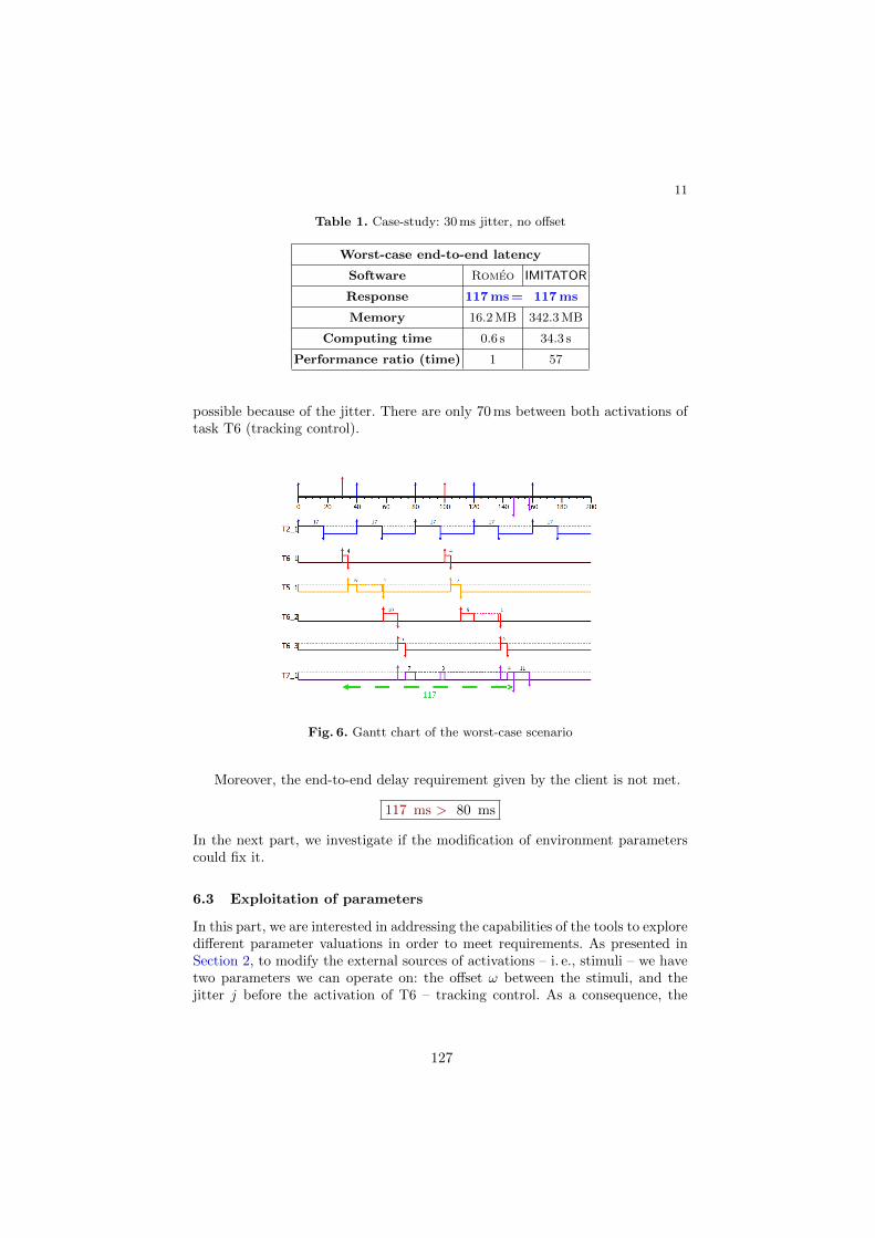
11
Table 1. Case-study: 30 ms jitter, no o↵set
Worst-case end-to-end latency
Software Romeo IMITATOR
Response 117 ms= 117 ms
Memory 16.2 MB 342.3 MB
Computing time 0.6 s 34.3 s
Performance ratio (time) 1 57
possible because of the jitter. There are only 70 ms between both activations oftask T6 (tracking control).
Fig. 6. Gantt chart of the worst-case scenario
Moreover, the end-to-end delay requirement given by the client is not met.
117 ms > 80 ms
In the next part, we investigate if the modification of environment parameterscould fix it.
6.3 Exploitation of parameters
In this part, we are interested in addressing the capabilities of the tools to exploredi↵erent parameter valuations in order to meet requirements. As presented inSection 2, to modify the external sources of activations – i. e., stimuli – we havetwo parameters we can operate on: the o↵set ! between the stimuli, and thejitter j before the activation of T6 – tracking control. As a consequence, the
127
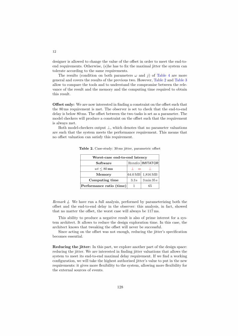
12
designer is allowed to change the value of the o↵set in order to meet the end-to-end requirements. Otherwise, (s)he has to fix the maximal jitter the system cantolerate according to the same requirements.
The results (condition on both parameters ! and j) of Table 4 are moregeneral and covers the results of the previous two. However, Table 2 and Table 3allow to compare the tools and to understand the compromise between the rele-vance of the result and the memory and the computing time required to obtainthis result.
O↵set only: We are now interested in finding a constraint on the o↵set such thatthe 80ms requirement is met. The observer is set to check that the end-to-enddelay is below 80 ms. The o↵set between the two tasks is set as a parameter. Themodel checkers will produce a constraint on the o↵set such that the requirementis always met.
Both model-checkers output ?, which denotes that no parameter valuationsare such that the system meets the performance requirement. This means thatno o↵set valuation can satisfy this requirement.
Table 2. Case-study: 30 ms jitter, parametric o↵set
Worst-case end-to-end latency
Software Romeo IMITATOR
wt 80 ms ? = ?Memory 64.0 MB 1,816 MB
Computing time 3.3 s 3 min 35 s
Performance ratio (time) 1 65
Remark 4. We have run a full analysis, performed by parameterizing both theo↵set and the end-to-end delay in the observer: this analysis, in fact, showedthat no matter the o↵set, the worst case will always be 117 ms.
This ability to produce a negative result is also of prime interest for a sys-tem architect. It allows to reduce the design exploration time. In this case, thearchitect knows that tweaking the o↵set will never be successful.
Since acting on the o↵set was not enough, reducing the jitter’s specificationbecomes essential.
Reducing the jitter: In this part, we explore another part of the design space:reducing the jitter. We are interested in finding jitter valuations that allows thesystem to meet its end-to-end maximal delay requirement. If we find a workingconfiguration, we will take the highest authorised jitter’s value to put in the newrequirements: it gives more flexibility to the system, allowing more flexibility forthe external sources of events.
128
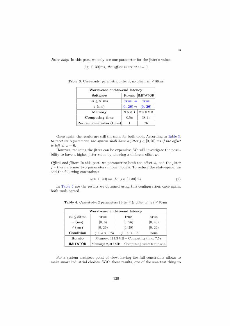
13
Jitter only: In this part, we only use one parameter for the jitter’s value:
j 2 [0, 30] ms, the o↵set is set at ! = 0
Table 3. Case-study: parametric jitter j, no o↵set, wt 80 ms
Worst-case end-to-end latency
Software Romeo IMITATOR
wt 80 ms true = true
j (ms) [0, 26), [0, 26)
Memory 9.6 MB 267.8 MB
Computing time 0.5 s 38.1 s
Performance ratio (time) 1 76
Once again, the results are still the same for both tools. According to Table 3:to meet its requirement, the system shall have a jitter j 2 [0, 26)ms if the o↵setis left at ! = 0.
However, reducing the jitter can be expensive. We will investigate the possi-bility to have a higher jitter value by allowing a di↵erent o↵set !.
O↵set and jitter: In this part, we parametrize both the o↵set !, and the jitterj – there are now two parameters in our models. To reduce the state-space, weadd the following constraints:
! 2 [0, 40) ms & j 2 [0, 30] ms (2)
In Table 4 are the results we obtained using this configuration: once again,both tools agreed.
Table 4. Case-study: 2 parameters (jitter j & o↵set !), wt 80 ms
Worst-case end-to-end latency
wt 80 ms true true true
! (ms) [0, 6) [0, 26) [0, 40)
j (ms) [0, 29) [0, 29) [0, 26)
Condition �j + ! > �23 �j + ! > �3 none
Romeo Memory: 117.3 MB – Computing time: 7.5 s
IMITATOR Memory: 2,017 MB – Computing time: 6 min 36 s
For a system architect point of view, having the full constraints allows tomake smart industrial choices. With these results, one of the smartest thing to
129

14
do in order to have worst time 80 ms is, for example, to use 6ms o↵set with28 ms jitter. These two values are allowed by the results model-checkers gave us,and it is one of the highest jitter we can have.
6.4 Tool comparison
In our experimentations, Romeo has always performed better than IMITATOR
in terms of time and memory consumption. Therefore, Romeo seems to be apromising tool for future industrial use. It would be interesting to know whythere is such a gap between these model-checkers, although they use a verysimilar notion of symbolic state, and a common internal representation usingthe Parma Polyhedra Library [9]. Here are some hypotheses:
– Both PSwAs and PSwPNs use clocks, i. e., real-valued variables. The numberof clocks significantly impacts the model checking performance. A main dif-ference is that clocks are created statically in PSwAs (hence in IMITATOR),whereas they are dynamic in PSwPNs (hence in Romeo) and are thereforefewer in this latter case.
– The reentrancy phenomenon is well managed in Romeo, thanks to the Petrinet theory – it is just multiple tokens in one place – whereas in IMITATOR,the reentrancy is made possible by adding variables and automata, whichnecessarily impacts the e�ciency.
In addition, note that the distributed capabilities of IMITATOR were not used inour comparison.
Nevertheless, IMITATOR and Romeo gave us the same results: this is crucialfor confidence in our results. Tool redundancy is used in some certification pro-cesses to lower the certification level needed for each tool. Having several toolswith distinct underlying techniques, formalisms, and libraries that output thesame results, can help in cheaper certifications.
7 Conclusion
In this paper, we faced a concrete industrial need concerning an aerial videotracking system made by THALES: can this system meet an additional end-to-end delay?
With our study, we used parametric model checking to investigate possibledesigns and answer this question. We used two di↵erent tools using formal meth-ods – IMITATOR and Romeo. By doing that, and checking certain properties onour models, we have now a precise idea of what we have to do to respect thisrequirement. Moreover, both tools drew the same conclusions: that is reassuring,both for these two tools and for our models. More important, it also validatesthe estimated performances presented in this paper.
This kind of approach was able to give us solutions to our questions. Even ifthere is no certification yet, this study allows to glimpse the potential of model-checking techniques using parameters for industrial use.
130
15
In the future, THALES R&D engineers want to promote the use of model-checking software for industrial practices, and implement it in design and analysistools already available. Therefore, the next step is to test the limitation of theselected tool: by creating models with a large pallet of specifications, and seeif the model-checker can manage every feature. If the tool passes the exam,there is an upscaling process: from any system modeled with THALES’ tool,automatically generate a model fit for our model-checker.
Acknowledgment
The authors would like to thank Violette Lecointre for her participation at mod-eling the case-study with Romeo.
References
1. L. Aceto, P. Bouyer, A. Burgueno, and K. G. Larsen. The power of reachabilitytesting for timed automata. In FSTTCS, volume 1530 of Lecture Notes in ComputerScience, pages 245–256. Springer, 1998.
2. L. Aceto, A. Burgueno, and K. G. Larsen. Model checking via reachability test-ing for timed automata. In TACAS, volume 1384 of Lecture Notes in ComputerScience, pages 263–280. Springer, 1998.
3. R. Alur, T. A. Henzinger, and M. Y. Vardi. Parametric real-time reasoning. InSTOC, pages 592–601. ACM, 1993.
4. E. Andre. Observer patterns for real-time systems. In ICECCS, pages 125–134.IEEE Computer Society, 2013.
5. E. Andre. What’s decidable about parametric timed automata? In FTSCS, vol-ume 596 of Communications in Computer and Information Science, pages 1–17.Springer, 2016.
6. E. Andre, Th. Chatain, E. Encrenaz, and L. Fribourg. An inverse method forparametric timed automata. International Journal of Foundations of ComputerScience, 20(5):819–836, Oct. 2009.
7. E. Andre, L. Fribourg, U. Kuhne, and R. Soulat. IMITATOR 2.5: A tool foranalyzing robustness in scheduling problems. In FM, volume 7436 of Lecture Notesin Computer Science, pages 33–36. Springer, 2012.
8. E. Andre, D. Lime, and O. H. Roux. Integer-complete synthesis for boundedparametric timed automata. In RP, volume 9058 of Lecture Notes in ComputerScience, pages 7–19. Springer, 2015.
9. R. Bagnara, P. M. Hill, and E. Za↵anella. The Parma Polyhedra Library: Toward acomplete set of numerical abstractions for the analysis and verification of hardwareand software systems. Science of Computer Programming, 72(1–2):3–21, 2008.
10. E. Bini. The Design Domain of Real-Time Systems. PhD thesis, Scuola SuperioreSant’Anna, 2004.
11. H. Boucheneb, G. Gardey, and O. H. Roux. TCTL model checking of time Petrinets. Journal of Logic and Computation, 19(6):1509–1540, 2009.
12. L. Doyen. Robust parametric reachability for timed automata. Information Pro-cessing Letters, 102(5):208–213, 2007.
131
16
13. M. Gonzalez Harbour, J. J. Gutierrez Garcıa, J. C. Palencia Gutierrez, and J. M.Drake Moyano. MAST: modeling and analysis suite for real time applications. InECRTS, pages 125–134. IEEE Computer Society, 2001.
14. R. Henia, A. Hamann, M. Jersak, R. Racu, K. Richter, and R. Ernst. System levelperformance analysis – the SymTA/S approach. IEE Proceedings – Computers andDigital Techniques, 152(2):148 – 166, 2005.
15. A. Jovanovic, D. Lime, and O. H. Roux. Integer Parameter Synthesis for Real-TimeSystems. IEEE Transactions on Software Engineering, 41(5):445–461, 2015.
16. T. T. H. Le, L. Palopoli, R. Passerone, and Y. Ramadian. Timed-automata basedschedulability analysis for distributed firm real-time systems: a case study. Inter-national Journal on Software Tools for Technology Transfer, 15(3):211–228, 2013.
17. D. Lime, O. H. Roux, C. Seidner, and L.-M. Traonouez. Romeo: A parametricmodel-checker for Petri nets with stopwatches. In TACAS, volume 5505 of LectureNotes in Computer Science, pages 54–57. Springer, 2009.
18. J. S. Miller. Decidability and complexity results for timed automata and semi-linear hybrid automata. In HSCC, volume 1790 of Lecture Notes in ComputerScience, pages 296–309. Springer, 2000.
19. J. C. Palencia Gutierrez and M. Gonzalez Harbour. Schedulability analysis fortasks with static and dynamic o↵sets. In IEEE Real-Time Systems Symposium,pages 26–37. IEEE Computer Society, 1998.
20. K. Richter and R. Ernst. Event model interfaces for heterogeneous system analysis.In DATE, pages 506–513. IEEE Computer Society, 2002.
21. Y. Sun, R. Soulat, G. Lipari, E. Andre, and L. Fribourg. Parametric schedulabilityanalysis of fixed priority real-time distributed systems. In FTSCS, volume 419 ofCommunications in Computer and Information Science, pages 212–228. Springer,2013.
22. L.-M. Traonouez, D. Lime, and O. H. Roux. Parametric model-checking of stop-watch Petri nets. Journal of Universal Computer Science, 15(17):3273–3304, 2009.
23. E. Wandeler, L. Thiele, M. Verhoef, and P. Lieverse. System architecture evalua-tion using modular performance analysis: a case study. International Journal onSoftware Tools for Technology Transfer, 8(6):649–667, 2006.
132
Parameterised Verification of StabilisationProperties via Conditional Spotlight Abstraction
Nils Timm and Stefan Gruner
Department of Computer Science, University of Pretoria, South Africa{ntimm,sgruner}@cs.up.ac.za
Abstract. Parameterised verification means to check properties of anarbitrary number of uniform processes composed in parallel. We intro-duce an approach to parameterised verification of stabilisation proper-ties. Our approach exploits the fact that stabilisation happens incre-mentally, and thus, also can be verified incrementally. We systematicallysearch for a provable partial stabilisation property and then verify fullstabilisation under the assumption of partial stabilisation. In order toprove partial stabilisation we use a novel stabilisation cuto↵ technique.A proven partial stabilisation property allows us to apply our new tech-nique conditional spotlight abstraction (CSA). CSA summarises an arbi-trary number of processes into a finite model such that verification canbe performed via model checking. Based on a prototype tool we wereable to verify several protocols implemented as parameterised systems.
1 Introduction
Parameterised systems consist of an unbounded number of uniform processesrunning in parallel in an asynchronous interleaving fashion. Practical examplescan be found in all sorts of distributed algorithms, like mutual exclusion or leaderelection. Such systems are often charged with safety-critical computations. Thus,techniques for establishing the correctness of parameterised systems are of greatimportance. Correctness is typically defined in terms of temporal logic prop-erties. Parameterised verification involves to check whether certain propertieshold regardless of the number of processes in the system, which is undecidablein general. Existing approaches are typically incomplete or restricted to certainproperties and classes of systems. Even if a method principally allows to solvea verification task, e�ciency is still a matter, since the practical applicability ofverification techniques is limited by the state explosion problem.
Here we introduce an automatic technique for parameterised verification ofstabilisation properties under fairness. Stabilisation is a liveness property andthus particularly hard to verify. It claims that all computations of a systemwill eventually reach a desired configuration and remain there forever. Hence,stabilisation can capture properties like the absence of deadlocks and livelocks,or the achievement of self-stabilisation in fault-tolerant systems. Our techniqueexploits the fact that stabilisation happens incrementally, and thus, also canbe verified incrementally. We first determine a provable partial stabilisation
133
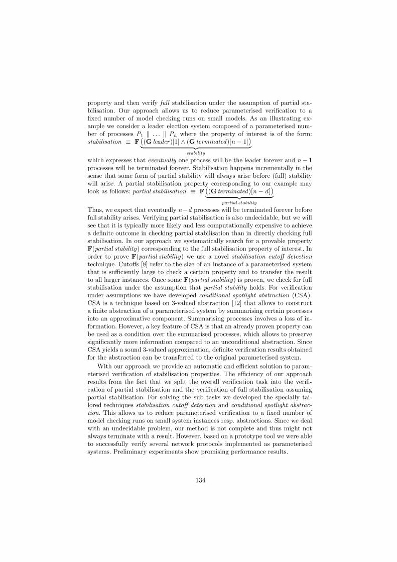
property and then verify full stabilisation under the assumption of partial sta-bilisation. Our approach allows us to reduce parameterised verification to afixed number of model checking runs on small models. As an illustrating ex-ample we consider a leader election system composed of a parameterised num-ber of processes P1 k . . . k Pn where the property of interest is of the form:stabilisation ⌘ F ((G leader)[1] ^ (G terminated)[n � 1])| {z }
stability
which expresses that eventually one process will be the leader forever and n � 1processes will be terminated forever. Stabilisation happens incrementally in thesense that some form of partial stability will always arise before (full) stabilitywill arise. A partial stabilisation property corresponding to our example maylook as follows: partial stabilisation ⌘ F ((G terminated)[n � d ])| {z }
partial stability
Thus, we expect that eventually n�d processes will be terminated forever beforefull stability arises. Verifying partial stabilisation is also undecidable, but we willsee that it is typically more likely and less computationally expensive to achievea definite outcome in checking partial stabilisation than in directly checking fullstabilisation. In our approach we systematically search for a provable propertyF(partial stability) corresponding to the full stabilisation property of interest. Inorder to prove F(partial stability) we use a novel stabilisation cuto↵ detectiontechnique. Cuto↵s [8] refer to the size of an instance of a parameterised systemthat is su�ciently large to check a certain property and to transfer the resultto all larger instances. Once some F(partial stability) is proven, we check for fullstabilisation under the assumption that partial stability holds. For verificationunder assumptions we have developed conditional spotlight abstraction (CSA).CSA is a technique based on 3-valued abstraction [12] that allows to constructa finite abstraction of a parameterised system by summarising certain processesinto an approximative component. Summarising processes involves a loss of in-formation. However, a key feature of CSA is that an already proven property canbe used as a condition over the summarised processes, which allows to preservesignificantly more information compared to an unconditional abstraction. SinceCSA yields a sound 3-valued approximation, definite verification results obtainedfor the abstraction can be transferred to the original parameterised system.
With our approach we provide an automatic and e�cient solution to param-eterised verification of stabilisation properties. The e�ciency of our approachresults from the fact that we split the overall verification task into the verifi-cation of partial stabilisation and the verification of full stabilisation assumingpartial stabilisation. For solving the sub tasks we developed the specially tai-lored techniques stabilisation cuto↵ detection and conditional spotlight abstrac-tion. This allows us to reduce parameterised verification to a fixed number ofmodel checking runs on small system instances resp. abstractions. Since we dealwith an undecidable problem, our method is not complete and thus might notalways terminate with a result. However, based on a prototype tool we were ableto successfully verify several network protocols implemented as parameterisedsystems. Preliminary experiments show promising performance results.
134
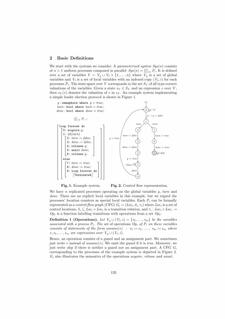
2 Basic Definitions
We start with the systems we consider. A parameterised system Sys(n) consistsof n > 1 uniform processes composed in parallel: Sys(n) = kn
i=1 Pi . It is definedover a set of variables V = Vg [ Vl ⇥ {1, . . . ,n} where Vg is a set of globalvariables and Vl is a set of local variables with an indexed copy (Vl , i) for eachprocesses Pi . The state space over V corresponds to the set SV of all type-correctvaluations of the variables. Given a state sV 2 SV and an expression e over V ,then sV (e) denotes the valuation of e in sV . An example system implementinga simple leader election protocol is shown in Figure 1.
y : semaphore where y = true;turn : bool where turn = true;done : bool where done = true;
kni=1 Pi ::
266666666666666666666664
loop forever do2666666666666666666664
0: acquire y ;1: if(turn)266664
2: turn := false;3: done := false;4: release y ;5: await done;6: release y ;
377775
else2664
7: turn := true;8: done := true;9: loop forever do⇥
Terminated⇤
3775
3777777777777777777775
377777777777777777777775
Fig. 1. Example system.
0
Gi
1
72
8
9
3
4
5
6
¬y
y ! y := false
¬done
skip
¬turn
turn := true
done := true
turn
turn := false
done := false
y := true
done
y := true
Fig. 2. Control flow representation.
We have n replicated processes operating on the global variables y , turn anddone. There are no explicit local variables in this example, but we regard theprocesses’ location counters as special local variables. Each Pi can be formallyrepresented as a control flow graph (CFG) Gi = (Loci , �i , ⌧i) where Loci is a set ofcontrol locations, �i ✓ Loci ⇥Loci is a transition relation, and ⌧i : Loci ⇥Loci !Opi is a function labelling transitions with operations from a set Opi :
Definition 1 (Operations). Let Vg [ (Vl , i) = {v1, . . . , vm} be the variablesassociated with a process Pi . The set of operations Opi of Pi on these variablesconsists of statements of the form assume(e) : v1 := e1, . . . , vm := em wheree, e1, . . . , em are expressions over Vg [ (Vl , i).
Hence, an operation consists of a guard and an assignment part. We sometimesjust write e instead of assume(e). We omit the guard if it is true. Moreover, wejust write skip if there is neither a guard nor an assignment part. A CFG Gi
corresponding to the processes of the example system is depicted in Figure 2.Gi also illustrates the semantics of the operations acquire, release and await .
135
We assume that a deterministic initialisation is given by an assertion ' = 'g ^Vni=1 'i over V such that 'g initialises the global variables and each 'i uniformly
initialises the counters and local variables of the processes. For our example weassume ' = (y ^ turn ^done ^Vn
i=1(loci = 0)) where loci is the location counterof Pi . A computation of a system corresponds to a sequence where in each stepone process is non-deterministically selected and the operation at its currentlocation is attempted to be executed. If the execution is not blocked by a guard,the variables are updated according to the assignment part and the processadvances to the consequent location. The overall state space S corresponds to thestate set over V combined with the possible locations, i.e. S = ⇥n
i=1 Loci ⇥SV .Hence, each s 2 S is a tuple s = hl1, . . . , ln , sV i where each li 2 Loci andsV 2 SV . As state space models we use Kripke structures (KS).
Definition 2 (Kripke Structure). A Kripke structure over a set of atomicpredicates AP is a tuple M = (S ,S0,R,L) where
– S is a set of states with a subset S0 ✓ S of initial states,
– R ✓ S ⇥ S is a total transition relation,
– L : S ⇥ AP ! {true, false} is a function labelling states with predicates.
A path ⇡ of a Kripke structure is an infinite sequence of states s0s1s2 . . . withs0 2 S0 and R(si , si+1). ⇡i denotes the i -th state of ⇡ whereas ⇡i denotes the i -thsu�x ⇡i⇡i+1⇡i+2 . . . of ⇡. Moreover, ⇧S0
M denotes the set of all paths starting inS0 of M . A system can be represented as a Kripke structure as follows:
Definition 3 (Systems as Kripke Structures). Let Sys(n) = kni=1 Pi be a
system over V where each Pi is given by a CFG Gi = (Loci , �i , ⌧i). Let Pred bea predicate set over V and let ' be an initialisation predicate. The correspondingKS is M = (S ,S0,R,L) over AP = Pred [ {(loci = j ) | i 2 [1..n], j 2 Loci} with
– S := ⇥ni=1 Loci ⇥ SV ,
– S0 := {s 2 S |s(') = true},– R(hl1 . . . , ln , sV i , hl 01 . . . , l 0n , s 0V i) :=Wn
i=1(Ri(hli , sV i , hl 0i , s 0V i) ^Vj 6=i(lj = l 0j ^
Vv2(Vl ,j )
sV (v) = s 0V (v)))whereRi(hli , sV i , hl 0i , s 0V i) = �i (li , l
0i ) ^ sV (e) ^Vm
k=1 s 0V (vk ) = sV (ek )assuming that ⌧i(li , l
0i ) = assume(e) : v1 :=e1, . . . , vm :=em ,
– L(hl1 . . . , ln , sV i , p) := sV (p) for any p 2 Pred,
– L (hl1 . . . , ln , sV i , (loci = j )) :=
⇢true if li = jfalse else
.
Representing a system as a KS typically involves the application of predicateabstraction [3]. Since our example system is solely defined over variables with aBoolean domain, we can directly take the variables as predicates, i.e. Pred := V .Paths of KS are considered for the evaluation of temporal logic properties. Herewe consider the temporal logic LTL.
136

Definition 4 (LTL Model Checking). Let M = (S ,S0,R,L) over AP be aKS. Then the evaluation of an LTL formula over AP on a path ⇡ 2 ⇧M ,written [⇡ |= ], is defined as follows
[⇡ |= p] := L(⇡0, p)
[⇡ |= ¬ ] := ¬ [⇡ |= ]
[⇡ |= ^ 0] := [⇡ |= ] ^ [⇡ |= 0]
[⇡ |= G ] :=V
i2N⇥⇡i |=
⇤
[⇡ |= F ] :=W
i2N⇥⇡i |=
⇤
[⇡ |= U 0] :=W
i2N
⇣[⇡i |= 0] ^V
0j<i [⇡j |= ]
⌘
Evaluating on entire KS is model checking: [M ,S0 |= ] :=V⇡2⇧S0
M[⇡ |= ].
Thus, given a system Sys(n), an initialisation predicate ', a set AP , and 2LTL, we can construct the corresponding KS M and check whether [M ,S0 |= ]holds. This tells us whether the system satisfies the property specified by ornot. For convenience, we typically just write [Sys(n),' |= ] when we refer tothe associated model checking problem. In parameterised verification one wantsto show that a property holds for all possible instances of a system:
8n > 1 : [Sys(n),'g ^Vni=1 'i |= ]
We implicitly assume strong fairness for all verification tasks, i.e. each operationthat is infinitely often enabled will be infinitely often executed:
fair ⌘ Vni=1
V(li ,l0i )2�i (GF (enabled(li , l
0i )) ! GF (executed(li , l
0i )))
Strong fairness guarantees that all processes always eventually proceed in a com-putation of a concurrent system. Fairness assumptions are essential in order toverify stabilisation properties under realistic conditions. In our approach we fo-cus on the stabilisation properties of the following form:
⌘ F ((G�1)[m1] ^ . . . ^ (G�k )[mk ])
where �1, . . . ,�k are predicate expressions over Vl and m1, . . . ,mk 2 N. Here wemake use of the following abbreviations:
Definition 5 (Abbreviations). Let Sys(n) be a system over V = Vg [ Vl ⇥{1, . . . ,n}. Let � be a predicate expression over Vl and m n. Then
�[m] ⌘ Wni1=1 . . .
Wnim=1(
Vmj=1 �ij )
(G�)[m] ⌘ Wni1=1 . . .
Wnim=1(
Vmj=1 G�ij )
assuming that i1, . . . , im pairwise disjoint.
Stabilisation is a crucial property for several kinds of parameterised systems.It claims that eventually a number of mi processes will be forever in a state
137
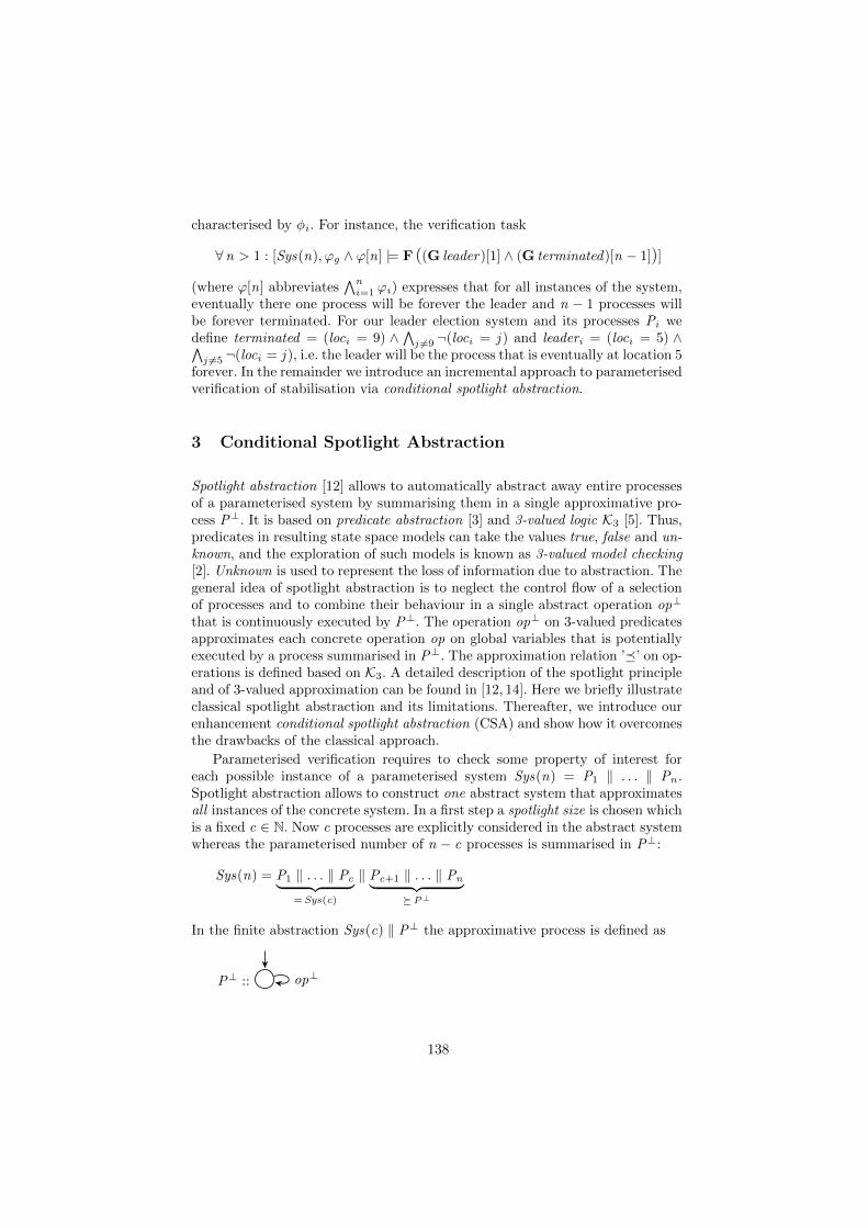
characterised by �i . For instance, the verification task
8n > 1 : [Sys(n),'g ^ '[n] |= F ((G leader)[1] ^ (G terminated)[n � 1])]
(where '[n] abbreviatesVn
i=1 'i) expresses that for all instances of the system,eventually there one process will be forever the leader and n � 1 processes willbe forever terminated. For our leader election system and its processes Pi wedefine terminated = (loci = 9) ^ V
j 6=9 ¬(loci = j ) and leaderi = (loci = 5) ^Vj 6=5 ¬(loci = j ), i.e. the leader will be the process that is eventually at location 5
forever. In the remainder we introduce an incremental approach to parameterisedverification of stabilisation via conditional spotlight abstraction.
3 Conditional Spotlight Abstraction
Spotlight abstraction [12] allows to automatically abstract away entire processesof a parameterised system by summarising them in a single approximative pro-cess P?. It is based on predicate abstraction [3] and 3-valued logic K3 [5]. Thus,predicates in resulting state space models can take the values true, false and un-known, and the exploration of such models is known as 3-valued model checking[2]. Unknown is used to represent the loss of information due to abstraction. Thegeneral idea of spotlight abstraction is to neglect the control flow of a selectionof processes and to combine their behaviour in a single abstract operation op?
that is continuously executed by P?. The operation op? on 3-valued predicatesapproximates each concrete operation op on global variables that is potentiallyexecuted by a process summarised in P?. The approximation relation ’�’ on op-erations is defined based on K3. A detailed description of the spotlight principleand of 3-valued approximation can be found in [12, 14]. Here we briefly illustrateclassical spotlight abstraction and its limitations. Thereafter, we introduce ourenhancement conditional spotlight abstraction (CSA) and show how it overcomesthe drawbacks of the classical approach.
Parameterised verification requires to check some property of interest foreach possible instance of a parameterised system Sys(n) = P1 k . . . k Pn .Spotlight abstraction allows to construct one abstract system that approximatesall instances of the concrete system. In a first step a spotlight size is chosen whichis a fixed c 2 N. Now c processes are explicitly considered in the abstract systemwhereas the parameterised number of n � c processes is summarised in P?:
Sys(n) = P1 k . . . k Pc| {z }=Sys(c)
k Pc+1 k . . . k Pn| {z }⌫P?
In the finite abstraction Sys(c) k P? the approximative process is defined as
P? :: op?
138
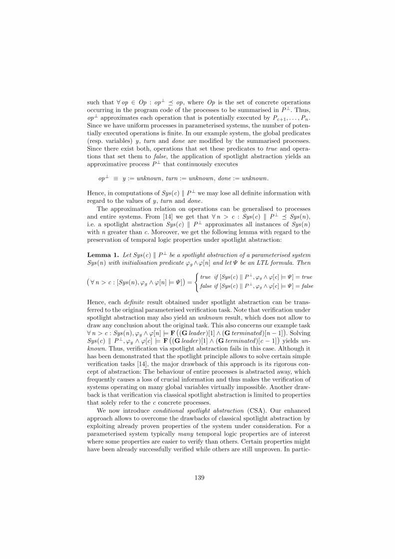
such that 8 op 2 Op : op? � op, where Op is the set of concrete operationsoccurring in the program code of the processes to be summarised in P?. Thus,op? approximates each operation that is potentially executed by Pc+1, . . . ,Pn .Since we have uniform processes in parameterised systems, the number of poten-tially executed operations is finite. In our example system, the global predicates(resp. variables) y , turn and done are modified by the summarised processes.Since there exist both, operations that set these predicates to true and opera-tions that set them to false, the application of spotlight abstraction yields anapproximative process P? that continuously executes
op? ⌘ y := unknown, turn := unknown, done := unknown.
Hence, in computations of Sys(c) k P? we may lose all definite information withregard to the values of y , turn and done.
The approximation relation on operations can be generalised to processesand entire systems. From [14] we get that 8n > c : Sys(c) k P? � Sys(n),i.e. a spotlight abstraction Sys(c) k P? approximates all instances of Sys(n)with n greater than c. Moreover, we get the following lemma with regard to thepreservation of temporal logic properties under spotlight abstraction:
Lemma 1. Let Sys(c) k P? be a spotlight abstraction of a parameterised systemSys(n) with initialisation predicate 'g ^'[n] and let be an LTL formula. Then
( 8n > c : [Sys(n),'g ^ '[n] |= ]) =
(true if [Sys(c) k P?,'g ^ '[c] |= ] = true
false if [Sys(c) k P?,'g ^ '[c] |= ] = false
Hence, each definite result obtained under spotlight abstraction can be trans-ferred to the original parameterised verification task. Note that verification underspotlight abstraction may also yield an unknown result, which does not allow todraw any conclusion about the original task. This also concerns our example task8n > c : Sys(n),'g ^ '[n] |= F ((G leader)[1] ^ (G terminated)[n � 1]). SolvingSys(c) k P?,'g ^ '[c] |= F ((G leader)[1] ^ (G terminated)[c � 1]) yields un-known. Thus, verification via spotlight abstraction fails in this case. Although ithas been demonstrated that the spotlight principle allows to solve certain simpleverification tasks [14], the major drawback of this approach is its rigorous con-cept of abstraction: The behaviour of entire processes is abstracted away, whichfrequently causes a loss of crucial information and thus makes the verification ofsystems operating on many global variables virtually impossible. Another draw-back is that verification via classical spotlight abstraction is limited to propertiesthat solely refer to the c concrete processes.
We now introduce conditional spotlight abstraction (CSA). Our enhancedapproach allows to overcome the drawbacks of classical spotlight abstraction byexploiting already proven properties of the system under consideration. For aparameterised system typically many temporal logic properties are of interestwhere some properties are easier to verify than others. Certain properties mighthave been already successfully verified while others are still unproven. In partic-
139

ular, we will see in a later section that checking stabilisation properties can bedone incrementally by first proving some form of partial stabilisation and secondchecking (full) stabilisation under the assumption of partial stabilisation. Thus,it is a realistic scenario that an LTL formula has to be verified assuming thatanother formula 0 holds. In fact, the initialisation predicate of a parameterisedsystem is a trivial form of such an assumption. While the initialisation predicateis inherently temporal operator-free, we now show that assumptions containingtemporal operators can be utilised to significantly increase the precision of thespotlight principle. Our CSA incorporates assumptions in the form of temporallogic formulas in the construction of the approximative process P?.
We start with an illustrating example for conditional spotlight abstraction.For our leader election system Sys(n) the LTL formula
0 ⌘ F ( (G terminated)[n � c] ^ 'g ^ '[c]| {z }=: 0
)
may have been already proven for some fixed c 2 N. Thus, we can assume thatfor all possible instances eventually n � c processes will be forever terminatedand c processes will be (still or again) in their initial configuration. The actualproperty of interest
⌘ F ( (G leader)[1] ^ (G terminated)[n � 1]| {z }=:
),
i.e. eventually exactly one leader forever, may be still unproven. For proving via CSA we make use of the following temporal logic inference rule:
(1) : 1 ! F 2
(2) : 2 ! F 3
(3) : 1 ! F 3
Thus, if, assuming 1, eventually 2 holds and, assuming 2, eventually 3
holds, then we can obviously conclude that, assuming 1, eventually 3 holds.In our example we have that (1): 8n > c : [Sys(n),'g ^ '[n] |= F 0] is alreadyproven, i.e., assuming 'g ^'[n], eventually 0 holds. Now we take 0 as the newinitialisation assumption and check whether F holds (2):
8n > c : P1 k ... k Pc| {z }Sys(c),'g ,'[c]
k Pc+1 k ... k Pn| {z }P?
G terminated
, (G terminated)[n � c] ^ 'g ^ '[c]| {z } 0
|= F
We see that the new initial condition 0 points at a spotlight abstraction withc concrete processes in their initial configuration and n � c processes to besummarised in P?. We additionally get from 0 that the summarised processesare terminated forever, which allows us to augment the summary process withthe condition G terminated where terminated = (loc = 9) ^ V
j 6=9 ¬(loc = j ).Hence, G terminated is a constraint on the control flow of each Pc+1 to Pn and
140
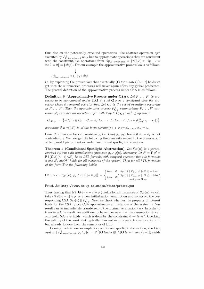
thus also on the potentially executed operations. The abstract operation op?
executed by P?G terminated only has to approximate operations that are consistent
with the constraint, i.e. operations from OpG terminated = {⌧(l , l 0) 2 Op | l =9^ l 0 = 9} = {skip}. For our example the approximative process looks as follows:
P?G terminated :: skip
i.e. by exploiting the proven fact that eventually (G terminated)[n � c] holds weget that the summarised processes will never again a↵ect any global predicates.The general definition of the approximative process under CSA is as follows:
Definition 6 (Approximative Process under CSA). Let P , . . . ,P 0 be pro-cesses to be summarised under CSA and let G� be a constraint over the pro-cesses where � temporal operator-free. Let Op be the set of operations occurringin P , . . . ,P 0. Then the approximative process P?
G� summarising P , . . . ,P 0 con-
tinuously executes an operation op? with 8 op 2 OpG� : op? � op where
OpG� = {⌧(l , l 0) 2 Op | Con{�, (loc = l) ^ (loc = l 0) ^ e ^Vmj=1(vj = ej )}}
assuming that ⌧(l , l 0) is of the form assume(e) : v1 :=e1, . . . , vm :=em .
Here Con denotes logical consistency, i.e. Con{�1,�2} holds if �1 ^ �2 is notcontradictory. We now get the following theorem with regard to the preservationof temporal logic properties under conditional spotlight abstraction:
Theorem 1 (Conditional Spotlight Abstraction). Let Sys(n) be a param-eterised system with initialisation predicate 'g ^'[n]. Moreover, let 0 = F 0 =F ((G�)[n�c]^�0) be an LTL formula with temporal operator-free sub formulae� and �0, and 0 holds for all instances of the system. Then for all LTL formulaeof the form F the following holds:
( 8n > c : [Sys(n),'g ^ '[n] |= F ]) =
(true if [Sys(c) k P?
G�,�0 |= F ] = true
false if
[Sys(c) k P?
G�,�0 |= F ] = false
and ! G¬ 0
!
Proof. See http://www.cs.up.ac.za/cs/ntimm/proofs.pdf
Thus, having that F ((G�)[n � c] ^ �0) holds for all instances of Sys(n) we cantake (G�)[n � c] ^ �0 as a new initialisation assumption and construct the cor-responding CSA Sys(c) k P?
G�. Next we check whether the property of interestholds for the CSA. Since CSA approximates all instances of the system, a trueresult can be immediately transferred to the original verification task. In order totransfer a false result, we additionally have to ensure that the assumption 0 canonly hold before holds, which is done by the constraint ! G¬ 0. Checkingthe validity of the constraint typically does not require an extra verification runbut already follows from the semantics of LTL.
Coming back to our example for conditional spotlight abstraction, checkingSys(c) k P?
G terminated ,'g^'[c] |= F ((G leader)[1]^(G terminated)[c�1]) yields
141
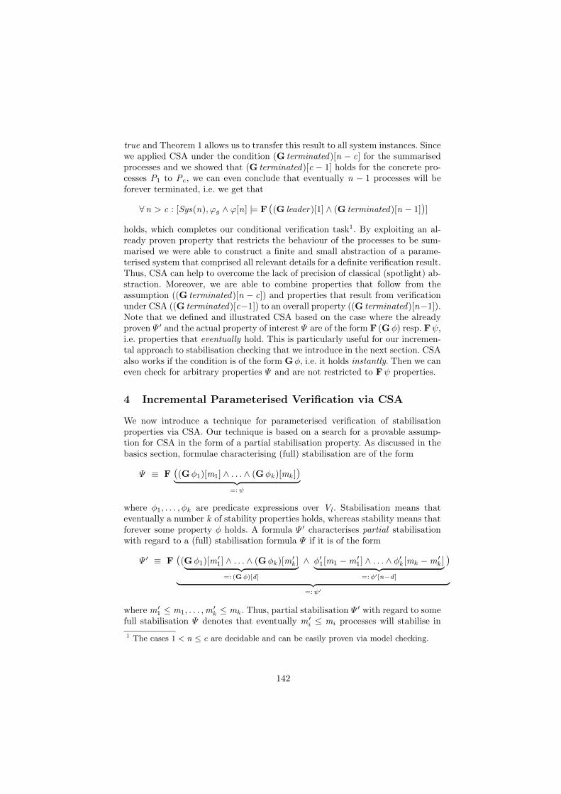
true and Theorem 1 allows us to transfer this result to all system instances. Sincewe applied CSA under the condition (G terminated)[n � c] for the summarisedprocesses and we showed that (G terminated)[c � 1] holds for the concrete pro-cesses P1 to Pc , we can even conclude that eventually n � 1 processes will beforever terminated, i.e. we get that
8n > c : [Sys(n),'g ^ '[n] |= F ((G leader)[1] ^ (G terminated)[n � 1])]
holds, which completes our conditional verification task1. By exploiting an al-ready proven property that restricts the behaviour of the processes to be sum-marised we were able to construct a finite and small abstraction of a parame-terised system that comprised all relevant details for a definite verification result.Thus, CSA can help to overcome the lack of precision of classical (spotlight) ab-straction. Moreover, we are able to combine properties that follow from theassumption ((G terminated)[n � c]) and properties that result from verificationunder CSA ((G terminated)[c�1]) to an overall property ((G terminated)[n�1]).Note that we defined and illustrated CSA based on the case where the alreadyproven 0 and the actual property of interest are of the form F (G�) resp. F ,i.e. properties that eventually hold. This is particularly useful for our incremen-tal approach to stabilisation checking that we introduce in the next section. CSAalso works if the condition is of the form G�, i.e. it holds instantly. Then we caneven check for arbitrary properties and are not restricted to F properties.
4 Incremental Parameterised Verification via CSA
We now introduce a technique for parameterised verification of stabilisationproperties via CSA. Our technique is based on a search for a provable assump-tion for CSA in the form of a partial stabilisation property. As discussed in thebasics section, formulae characterising (full) stabilisation are of the form
⌘ F ((G�1)[m1] ^ . . . ^ (G�k )[mk ])| {z }=:
where �1, . . . ,�k are predicate expressions over Vl . Stabilisation means thateventually a number k of stability properties holds, whereas stability means thatforever some property � holds. A formula 0 characterises partial stabilisationwith regard to a (full) stabilisation formula if it is of the form
0 ⌘ F ((G�1)[m01] ^ . . . ^ (G�k )[m 0
k ]| {z }=: (G�)[d]
^ �01[m1 � m 01] ^ . . . ^ �0k [mk � m 0
k ]| {z }=:�0[n�d]
)
| {z }=: 0
where m 01 m1, . . . ,m
0k mk . Thus, partial stabilisation 0 with regard to some
full stabilisation denotes that eventually m 0i mi processes will stabilise in
1 The cases 1 < n c are decidable and can be easily proven via model checking.
142
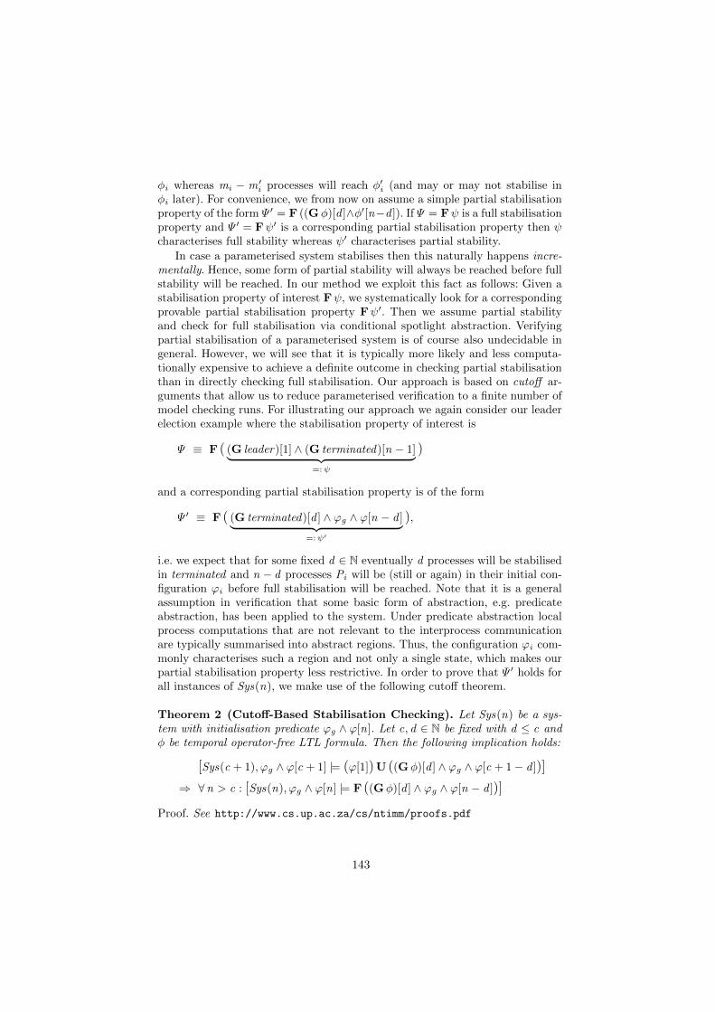
�i whereas mi � m 0i processes will reach �0i (and may or may not stabilise in
�i later). For convenience, we from now on assume a simple partial stabilisationproperty of the form 0 = F ((G�)[d ]^�0[n�d ]). If = F is a full stabilisationproperty and 0 = F 0 is a corresponding partial stabilisation property then characterises full stability whereas 0 characterises partial stability.
In case a parameterised system stabilises then this naturally happens incre-mentally. Hence, some form of partial stability will always be reached before fullstability will be reached. In our method we exploit this fact as follows: Given astabilisation property of interest F , we systematically look for a correspondingprovable partial stabilisation property F 0. Then we assume partial stabilityand check for full stabilisation via conditional spotlight abstraction. Verifyingpartial stabilisation of a parameterised system is of course also undecidable ingeneral. However, we will see that it is typically more likely and less computa-tionally expensive to achieve a definite outcome in checking partial stabilisationthan in directly checking full stabilisation. Our approach is based on cuto↵ ar-guments that allow us to reduce parameterised verification to a finite number ofmodel checking runs. For illustrating our approach we again consider our leaderelection example where the stabilisation property of interest is
⌘ F ( (G leader)[1] ^ (G terminated)[n � 1]| {z }=:
)
and a corresponding partial stabilisation property is of the form
0 ⌘ F ( (G terminated)[d ] ^ 'g ^ '[n � d ]| {z }=: 0
),
i.e. we expect that for some fixed d 2 N eventually d processes will be stabilisedin terminated and n � d processes Pi will be (still or again) in their initial con-figuration 'i before full stabilisation will be reached. Note that it is a generalassumption in verification that some basic form of abstraction, e.g. predicateabstraction, has been applied to the system. Under predicate abstraction localprocess computations that are not relevant to the interprocess communicationare typically summarised into abstract regions. Thus, the configuration 'i com-monly characterises such a region and not only a single state, which makes ourpartial stabilisation property less restrictive. In order to prove that 0 holds forall instances of Sys(n), we make use of the following cuto↵ theorem.
Theorem 2 (Cuto↵-Based Stabilisation Checking). Let Sys(n) be a sys-tem with initialisation predicate 'g ^ '[n]. Let c, d 2 N be fixed with d c and� be temporal operator-free LTL formula. Then the following implication holds:
[Sys(c + 1),'g ^ '[c + 1] |= ('[1])U ((G�)[d ] ^ 'g ^ '[c + 1 � d ])]
) 8n > c : [Sys(n),'g ^ '[n] |= F ((G�)[d ] ^ 'g ^ '[n � d ])]
Proof. See http://www.cs.up.ac.za/cs/ntimm/proofs.pdf
143
A cuto↵ refers to the size of an instance that is su�ciently large to check a certainproperty of interest and to transfer the result to all larger instances as well. Weadapt this concept as follows: If a parameterised system satisfies some partialstabilisation property F 0, then under all possible executions a state satisfying 0 will be reached within a finite number of computational steps. Hence, only alimited number of processes can be actively involved in a computation reaching 0. Let c be this number, then an instance of size c + 1 is obviously a cuto↵.In order to determine the maximum number of processes that can be involvedin reaching 0, we strengthen the partial stabilisation formula as follows: Wereplace F 0 (which is equivalent to true U 0) by '[1]U 0. If we can prove thestronger formula '[1]U 0 for a fixed instance of size c +1 this tells us that F 0
holds and there will be always at least one process in its initial region until 0
holds. We can conclude that c is the maximum number of processes that can beinvolved in a computation reaching 0, and since F 0 holds for a system withc + 1 processes we can transfer this result to any larger instance as well.
In comparison to existing techniques e.g. [4, 7, 9] that detect cuto↵s based onan analysis of the local state space of processes, we follow a di↵erent approach:We integrate cuto↵ detection into the verification task, i.e. we strengthen theproperty of interest such that we will only obtain a true result if we are usingan admissible cuto↵ and the property of interest holds for the cuto↵ instance.
The following procedure illustrates how we iteratively search for a provablepartial stabilisation property:
for c = 1 to 1 dofor d = 1 to c do
if Sys(c + 1),'g ^ '[c + 1] |= ('[1])U ((G�)[d ] ^ 'g ^ '[c + 1 � d ])then
return 8n > c : Sys(n),'g ^ '[n] |= F ((G�)[d ] ^ 'g ^ '[n � d ])
For our example the procedure terminates for c = 2 and d = 1. Hence, we get
8n > 2 : Sys(n),'g ^ '[n] |= F ((G terminated)[1] ^ 'g ^ '[n � 1])
This result points at a CSA with one terminated process to be summarisedand n � 1 concrete processes. Since the number of concrete processes wouldbe still parameterised, the application of CSA would so far not give us a finiteabstraction. However, we will now see that partial stabilisation results can beeasily expanded such that they point at expedient CSAs. In expanding the resultwe already make use of the conditional spotlight principle: We need to showthat the partial stabilisation property 0 also holds when we extend Sys(n) byan approximative component. In the same manner we have proven 0 for allinstances of Sys(n) via the cuto↵ theorem, we can also show the following:
8n > 2 : Sys(n) k P?G terminated ,'g ^ '[n] |= F ((G terminated)[1] ^ 'g ^ '[n � 1])
If partial stabilisation 0 has been proven for both, systems with and without anapproximative component then we can apply the following theorem that givesus the expanded partial stabilisation result:
144
Theorem 3 (Expanding Partial Stabilisation Results). Let Sys(n) be asystem with initialisation predicate 'g ^ '[n]. Let c, d 2 N be fixed with d cand � be temporal operator-free LTL formula. Then the following holds:
8n > c : [Sys(n),'g ^ '[n] |= F ((G�)[d ] ^ 'g ^ '[n � d ])]
^ 8n > c : [Sys(n) k P?G�,'g ^ '[n] |= F ((G�)[d ] ^ 'g ^ '[n � d ])]
) 8n > c : [Sys(n),'g ^ '[n] |= F ((G�)[n � f ] ^ 'g ^ '[f ])]
where f = (n mod d) + c + 1 � d (which also means 1 f c).
Proof. See http://www.cs.up.ac.za/cs/ntimm/proofs.pdf
In the proof we make use of the fact that Sys(n) will eventually reach a configura-tion corresponding to Sys(n�d) k P?
G�, which will in turn reach a configuration
corresponding to Sys(n�d �d) k P?G� and so on, until we reach a configuration
where the number of non-stabilised processes is f with 1 f c and the num-ber of stabilised processes is n � f which is a multiple of d . Thus, from Theorem3 we get that partial stabilisation of d processes implies partial stabilisation ofn � f processes. For our running example we get f = 2, i.e.
8n > 2 : [Sys(n),'g ^ '[n] |= F ( (G terminated)[n � 2]| {z }P?
G�
^ 'g ^ '[2]| {z }Sys(2),'g^'[2]
)]
The expanded result points at a CSA where we summarise the parameterisednumber of stabilised processes in the approximative component. Via CSA we nowcan check for full stabilisation F ((G leader)[1] ^ (G terminated)[n � 1]). Sincethe stabilisation of n � 2 processes in terminated is part of the already provenassumption, it only remains to show that
Sys(2) k P?G�,'g ^ '[2] |= F ((G leader)[1] ^ (G terminated)[1])
holds. Checking this decidable task yields true and the CSA theorem from Sec-tion 3 allows us to conclude that also
8n > 2 : [Sys(n),'g ^ '[n] |= F ((G leader)[1] ^ (G terminated)[n � 1])]
holds, which successfully completes our parameterised verification task. For otherverification tasks f (which is defined as (nmodd)+c+1�d) may be not distinctbut restricted to values from the typically very small set {1, . . . , c}. This reflectsthe fact that the extent of partial stabilisation may depend on the instance size n.In this case we have to check for full stabilisation via CSA for all f 2 {1, . . . , c}.
In summary, our technique for parameterised verification of stabilisationworks as follows: Given a system Sys(n) and a stabilisation property F , we sys-tematically search for a corresponding partial stabilisation property F 0 thatcan be proven for both Sys(n) and Sys(n) k P?
G � via our cuto↵ techniquewith property strengthening (Theorem 2). Next, we apply stabilisation expan-sion (Theorem 3) which yields an expanded property F 00 that also holds for
145

Sys(n). Finally, we use 00 as the assumption for CSA, which gives us a finite ab-straction on which we can check F . Theorem 1 allows us to transfer the resultto all instances of Sys(n) that are greater than the cuto↵. Since we deal withan undecidable problem, our approach is incomplete in the sense that the searchfor a partial stabilisation property might not terminate or CSA-based modelchecking might return unknown. However, in preliminary experiments we wereable to successfully verify several example systems implementing leader election.
5 Related Work
Our technique is related to a number of existing approaches to parameterisedverification. The cuto↵ concept was introduced in [4] where it was shown thatfor the verification of certain properties there exist cuto↵s that are polynomialin the number of local states of processes. Other cuto↵ approaches impose re-strictions on the communication scheme, e.g. only lock-based communication [7],and thus do not support the verification of systems with shared-variable concur-rency. [8] introduces dynamic cuto↵ detection during verification. The approachhas no restrictions on communication but is limited to safety properties. Tothe best of our knowledge, we are the first to integrate cuto↵ detection into theverification task by strengthening the property to be checked with a cuto↵ condi-tion. Verification of stabilisation has been considered in [6, 10, 11]. [6] presents asemi-automatic strategy for stabilisation checking that requires a user-providedfunction on states measuring the progress of computation towards stabilisation.In [10] an approach to the verification of convergence in self-stabilising protocolsis proposed. It is based on the derivation of convergence proofs. Convergence isa necessary but not su�cient condition for stabilisation. In [11] a verificationtechnique for stabilisation in population protocols is presented. The technique isbased on modelling the possible actions of the protocol whereas actual processesare not part of the model. All these approaches for stabilisation checking performverification on the basis of an algorithmic description of a protocol. In contrast,we focus on the verification of systems that implement protocols in a C-like lan-guage. Since the implementation of a protocol may introduce errors that are notpresent in the algorithmic description, a distinct verification of implementationsis indispensable. (Unconditional) spotlight abstraction was introduced in [12, 14].While the original technique is not capable of verifying stabilisation, our exten-sion to CSA has closed this gap. Another related approach is conditional modelchecking [1]. Here properties are checked under conditions that restrict whichpart of the model is explored. In contrast, we use conditions in order to abstractaway processes while preserving relevant information about their behaviour.
6 Conclusion and Outlook
We introduced an automatic technique for parameterised verification of stabili-sation, which is a vital property in many safety-critical systems. Our techniquereduces parameterised verification to a finite number of abstraction-based model
146
checking runs. One of our key concepts is incremental verification by first provingpartial stabilisation, and then checking for full stabilisation under the assumptionof partial stabilisation. The approach profits from the fact that proving partialstabilisation naturally requires smaller cuto↵s and thus less computational e↵ortthan directly proving full stabilisation. Our conditional spotlight abstraction al-lows us to exploit already proven properties in order to construct a small abstractmodel that still preserves relevant information about the system. Stabilisationcuto↵ detection and CSA are not limited to stabilisation checking. The cuto↵ ap-proach also works for arbitrary properties of the form F . CSA can also be usedfor other forms of conditional verification. Moreover, our approach can be gen-eralised to the verification of systems with di↵erent classes of uniform processes(class-wise symmetric systems) and to systems extended by individual processeslike daemons modelling potential faults. We implemented our technique on topof our 3-valued model checker [13] with strong fairness. Preliminary experimentsshow promising performance results. With our tool we could verify stabilisationof several leader election protocols implemented as parameterised systems. Anexperimental evaluation based on wireless sensor networks is in preparation.
Acknowledgements. We thank Mike Poppleton for fruitful discussions in thecontext of this paper.
References
1. Beyer, D., Henzinger, T.A., Keremoglu, M.E., Wendler, P.: Conditional modelchecking. In: ACM SIGSOFT FSE. pp. 57:1–57:11. ACM, New York (2012)
2. Bruns, G., Godefroid, P.: Model checking partial state spaces with 3-valued tem-poral logics. In: CAV 1999. pp. 274–287. LNCS, Springer Berlin Heidelberg (1999)
3. Clarke, E., Kroening, D., Sharygina, N., Yorav, K.: SATABS: SAT-based predicateabstraction for ANSI-C. In: TACAS. pp. 570–574. Springer (2005)
4. Emerson, E.A., Kahlon, V.: Reducing model checking of the many to the few. In:CADE. pp. 236–254. Springer (2000)
5. Fitting, M.: Kleene’s three valued logics and their children. Fundamenta Informat-icae 20(1-3), 113–131 (1994)
6. Ghosh, R., Mitra, S.: A strategy for automatic verification of stabilization of dis-tributed algorithms. In: FORTE. pp. 35–49. Springer (2015)
7. Kahlon, V., Ivancic, F., Gupta, A.: Reasoning about threads communicating vialocks. In: CAV. pp. 505–518. Springer (2005)
8. Kaiser, A., Kroening, D., Wahl, T.: Dynamic cuto↵ detection in parameterizedconcurrent programs. In: CAV. pp. 645–659. Springer (2010)
9. Kouvaros, P., Lomuscio, A.: A cuto↵ technique for the verification of parameterisedinterpreted systems with parameterised environments. In: IJCAI. Citeseer (2013)
10. Oehlerking, J., Dhama, A., Theel, O.: Towards automatic convergence verificationof self-stabilizing algorithms. In: SSS. pp. 198–213. Springer (2005)
11. Pang, J., Luo, Z., Deng, Y.: On automatic verification of self-stabilizing populationprotocols. Frontiers of Computer Science in China 2(4), 357–367 (2008)
12. Schrieb, J., Wehrheim, H., Wonisch, D.: Three-valued spotlight abstractions. In:Cavalcanti, A., Dams, D. (eds.) FM, LNCS, vol. 5850, pp. 106–122. Springer (2009)
147

13. Timm, N., Gruner, S., Harvey, M.: A bounded model checker for three-valuedabstractions of concurrent software systems. In: Proceedings of the 19th BrazilianSymposium on Formal Methods. Springer (2016)
14. Timm, N., Wehrheim, H.: On symmetries and spotlights – verifying parameterisedsystems. In: Dong, J., Zhu, H. (eds.) ICFEM, LNCS, vol. 6447, pp. 534–548.Springer (2010)
148


