Fig. 4.6. Fickian release kinetics. The dimensionless amount of drug released Mt+ increases

with the square root of the dimensionless time t+ in the range 0.2 < Mt+< 0.6 (release from

slab. Dashed line represents a 0.5 sloped curve). In the case of release from cylinder and sphere, Mt

+ (t+)0.45 and Mt+ (t+)0.43 would occur, respectively.

0.1

1

0.01 0.1 1

t+

Mt+

Fig. 4.7. Effect of the release environment volume on drug release from a slab. For increasing values of the ratio Rv (= matrix volume/ release environment volume) drug release kinetics detaches from the classical fickian kinetics represented by the grey curve (Rv = 0). Indeed, sink conditions no longer hold. In addition, only a fraction of the initial drug load can be released.

0.01

0.1

1

1 10 100 1000t +

Mt0

+

Rv = 0

Rv = 0.5

Rv = 1

Rv = 2

Fig. 4.8. Effect of partitioning at the matrix/release environmet interface assuming equality between matrix and release environmet volumes (Rv = 1). Partition coefficient kp increase exalts the deviation from the macroscopic fickian release and it further reduces the initial drug load that can be released.

0.01

0.1

1

1 10 100 1000t +

Mt0

+

kp = 1

kp = 2

kp = 10

Fig. 4.9. Effect of one step initial drug distribution (see insert) on drug release kinetics from a sphere. As step position (c) detaches from one (uinform drug distribution), a neat macroscopic non fickian behaviour appears.

0.01

0.1

1

0.001 0.01 0.1 1t +

Mt+

c=1

c=0.9

c=0.75

c=0.4

0

0.2

0.4

0.6

0.8

1

1.2

0 0.5 1 (-)

C+ (-

)

=c

Fig. 4.10. Effect of one step initial drug distribution on time evolution of Mt+ time (t+)

derivative. As step position (c) decreases, smoother Mt+ time derivative occurs.

0

5

10

15

20

25

30

0 0.05 0.1 0.15 0.2 0.25t +

dMt+

/dt+

c=1

c=0.9

c=0.75

c=0.4

Fig. 4.11. Effect of increasing, maximum and decreasing initial drug distribution (see insert) on drug release kinetics from a sphere. Release kinetics is heavily influenced by the ditsribution features. Maximum and decreasing distribution yield to a macroscopic non fickian behaviour.

0.1

1

0.001 0.01 0.1 1t +

Mt+

increasing

uniform

maximum

decreasing

0

0.2

0.4

0.6

0.8

1

1.2

0 0.5 1 (-)

C+ (-

)

Fig. 4.12. Effect of increasing, maximum and decreasing initial drug distribution on time evolution of Mt

+ time (t+) derivative. Smoother Mt+ time derivative occur for decreasing and

maximum distribution.

0.1

1

10

100

0 0.05 0.1 0.15 0.2 0.25t +

dMt+

/dt+

increasing

uniform

maximum

decreasing

Fig. 4.13. Effect of finite release environment volume assuming a decreasing stepwise initial drug concentration distribution (see insert in Fig. 4.11). The effect of finite release environment volume is evaluated through the parameter appearimg in eq.(4.165).

0

0.1

0.2

0.3

0.4

0.5

0.6

0.7

0.8

0.9

1

0 0.05 0.1 0.15 0.2 0.25t +

Mt0

+

=

= 10

= 2

= 0.5

Fig. 4.14. Effect of stagnant layer presence on drug release kinetics from a slab. Rsm indicates the ratio between stagnant layer and matrix thickness, while Dsl = 0.1*Dd0.

0.01

0.1

1

1 10 100 1000

t +

Mt+ Rsm = 0

Rsm = 0.2

Rsm = 0.05

Fig. 4.15. Effect of stagnant layer presence on drug release kinetics from a slab. Rsm indicates the ratio between stagnant layer and matrix thickness. The simulation is performed assuming that the diffusion coefficient in the stagnant layer is equal to that in the matrix (Dsl = Dd0).

0.01

0.1

1

10 100 1000 10000

t +

Mt+

R sm = 0

R sm =

0.05

R sm =

0.2

Fig. 4.16. Schematic representation of the cylindrical matrix coated by an impermeable holed membrane on its bottom plane surface. This picture also shows the boundary conditions for eq.(4.189) solution in the hypothesis of reducing the three-dimensions problem to a simpler two-dimensions problem.

r m

Cylinder

r h

Holed membrane

hc

2b

0m2

rYY

C

00

YY

C

00

X

XC

C = 0

C = 0

C = 0

C = 0

C = 0

X

Y

0c

hXX

C

0c

hXX

C

Fig. 4.17. Effect of membrane void fraction assuming the exixtence of only one hole. The smaller , the more pronounced the macroscopic non fickian character of the release curve. The simulation is performed assuming a square system (hc = 2rm).

0.01

0.1

1

0.001 0.01 0.1 1 10

t +

Mt+

Fig. 4.18. Effect of Nf (or rh/rm) variation, once has been fixed. Higher Nf favours drug release (see dotted line). = 1 curve is reported as refernce (fickian kinetics). The simulation is performed assuming a square system (hc = 2rm).

0.01

0.1

1

0.001 0.01 0.1 1 10

t +

Mt+

= 1, Nf = 1

= 0.5, Nf = 1

= 0.5, Nf = 10

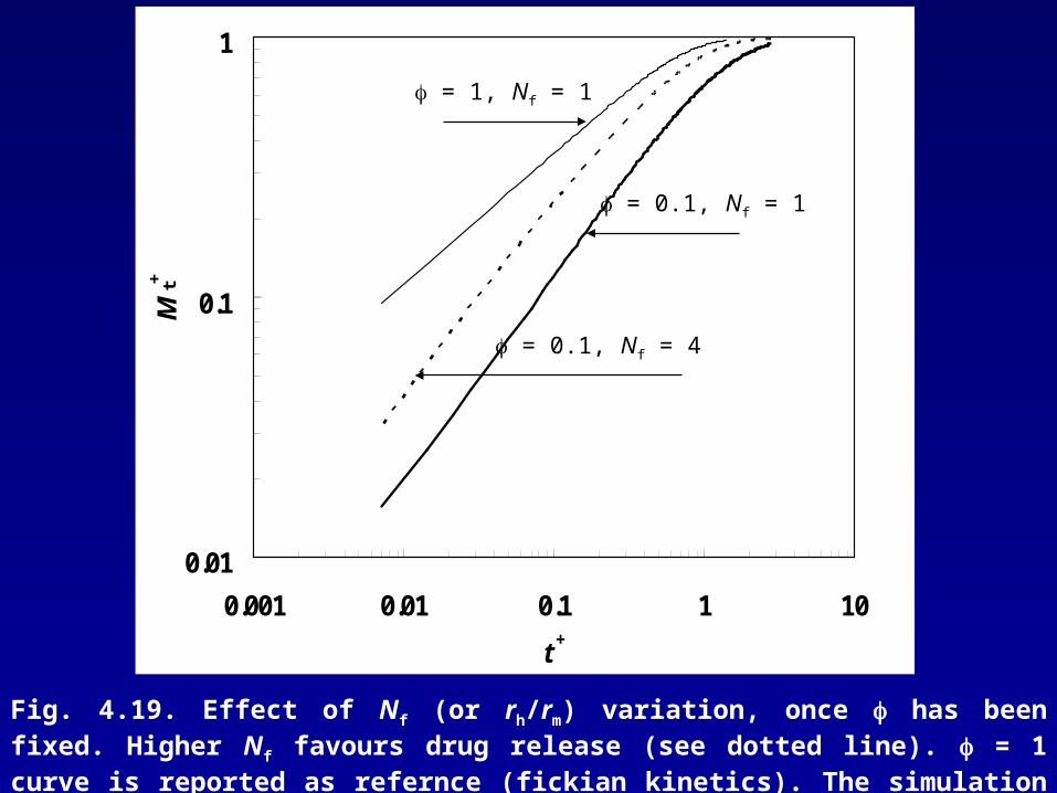
Fig. 4.19. Effect of Nf (or rh/rm) variation, once has been fixed. Higher Nf favours drug release (see dotted line). = 1 curve is reported as refernce (fickian kinetics). The simulation is performed assuming a square system (hc = 2rm).

0.01

0.1

1

0.001 0.01 0.1 1 10

t +

Mt+

= 1, Nf = 1

= 0.1, Nf = 1

= 0.1, Nf = 4

1

C+

0

0

0.78

1

1

Y+ = Y/2rm

X+ = X/hc

Fig. 4.20. Dimesionless concentration surface C+(X+, Y+) assuming = 0.5, Nf = 3 (rh/rm = 0.167), hc/2rm = 1, sink conditions and t+ = 0.0027, corresponding to Mt

+ = 0.0365.

Fig. 4.21. Effect of the hc/2rm ratio variation on drug release assuming = 0.5 and Nf = 1.

0.01

0.1

1

0.001 0.01 0.1 1 10

t +

Mt+

hc/2rm = 0.5

hc/2rm = 1

hc/2rm = 2

b

rh

h(t)

k*h(t)

Va

Y

ZVb

Fig. 4.22. Time evolution of the diffusion front according to the Buchtel model. The front develops as a half rotational ellipsoid having height h(t) and radius (rh + k*h(t)). When vessel wall or adjacent holes diffusion fronts met, the diffusion front surface results from the intersection between the ellipsoid and a cylinder of radius (rh + b). In the Pywell and Collet approach [62], instead, the diffusion front surface is a segment of sphere having height h and cord 2*(rh + h). Accordingly, its shape is more squeezed than the Buchtel one and its centre, lying on the Z axis, approaches hole surface as h increases.

Fig. 4.23. Comparison between Buchtel model (thick line) and numeric solution (thin line) (eq.(4.189)) assuming D = 10-6 cm2/s, = 0.5, rm = 2263 m (hfin = 2263 m) mm, 2 holes and k = 0.5 . A satisfactory agreement holds up to Mt

+ ≈ 0.4.

0

0.1

0.2

0.3

0.4

0.5

0.6

0 0.1 0.2 0.3

t +

Mt+

Buchtel

Numeric (eq.(4.189))

Fig. 4.24. Time evolution of the diffusion front according to the Buchtel model in the case of two holes. The parameter used in this simulation are the same used in Figure 4.23.

t+ = 7.1*10

-2

t+ = 1.1*10

-3

t+ = 2.7*10

-3

t+ = 8.8*10

-3

t+ = 2.7*10

-2

t+ =1.8*10

-4