FILE COpyDO NOT REMOVE

NSTTUTE FOR 142-72

--;;

RESEARCH ONPOVERTYD'SCWK?~~~

THE DISTRIBUTIONAL IMPLICATIONS OFAGRICULTURAL COMMODITY PROGRAMS

Russell Lidman

~----~---_._--.~_.._---

THE DISTRIBUTIONAL IMPLICATIONS OFAGRICULTURAL COMMODITY PROGRAMS

Russell Lidman

The author of this paper is an Institute Research Associate at theInstitute for Research on Poverty, University of Wisconsin-Madison.Much of the work on which this paper was based was done in connectionwith the author's Ph.D. thesis, liThe Distribution of Benefit of MajorAgricultural Commodity Programs: A Case Study of 1969" (University ofWisconsin-Madison, 1972). The assistance of -Dr'. Robert Posner, ProfessorD. Lee Bawden) and numerous others is gratefully acknowledged.

The research reported here was supported in part by funds granted to theInstitute for Research on Poverty at the University of Wisconsin by theOffice of Economic Opportunity pursuant to the provisions of the EconomicOpportunity Act of 1964. The author is solely responsible for theconclusions.

September 1972

ABSTRACT

This paper examines agricultural commodity programs primarily from

the perspective of their distributional implications among producers. Farm

programs have a minor effect on the distribution of income among these

units. At the very most about $500 million or about 10 percent of the

total long-run annual benefits of farm programs accrues to approximately

29 percent of the total farm operator population who are poor.

Furthermore, farm-program benefits supplement the total income of the

agricultural poor by a relatively small amount. Benefits are only 4

percent of total income for operators of the smallest sized units. The

comparable figure for operators of' the largest units is 25 percent.

Because of the way they are structured, the benefits of farm programs

by-pass the landless in agriculture--for example, hired hands, migrant workers,

tenants and sharecroppers. In addition, the structure of farm programs

virtually dictates that the benefits become capitalized into land values.

This means that even current landowners may receive a small share of the

intended benefits. Previous landowners in many cases have received some

part of the discounted value of future farm-program benefits by selling the

land at elevated prices to the current generation of operators.

Though farm programs have other goals aside from income maintenance,

they remain as one of the foremost mechanisms addressed to the rural poverty

problem. They are out of date and inadequate for the task. Even recent

reforms, such as payment limitations, offer little scope for improvement

since they do not affect the basic mechanisms of the programs--and it is

these mechanisms which must be substantially altered.

THE DISTRIBUTIONAL IMPLICATIONS OF

AGRICULTURAL COMMODITY PROGRAMS

Russell Lidman

INTRODUCTION

This paper examines agricultural commodity programs primarily from the

point of view of the implications of these programs on income distribution

among producers. From a brief historical introduction to agricultural

policy it is shown that U.S. policies have considerable precedent. The

examination of U.S. practices outlines the evolution of policy from the

New Deal, when direct intervention was initiated.

Considerable attention is devoted to analyzing the mechanisms of supp1y­

control programs. The wheat program is used as an illustration. Current

mechanisms of supply-control were developed in part by an empirical approach-­

trial and error. For example, government purchases and consequently the large

publicly owned surplus of the late 1950s demonstrated the pitfalls of a

high loan rate and inadequate incentive to divert acreage from production.

Consequently policies after the mid-1960s emphasized low loan rates, sub­

stantial direct payments for participating,. and.the opportunity to voluntarily

divert additional. acreage for payment.

An analysis of the potentia~ effects of commodity programs on farmers'

income demonstrates some of the shortcomings of the present technique. The

benefits of U.S. farm programs tend to be capitalized into land values; farm

programs are in part responsible for the dramatic increases in land prices

over the last 40 years. Since these benefits of farm programs represent

returns to land ownership, this mechanism offers insignificant income

assistance to the landless, for example hired farmworkers and tenants.

~~~-~"-~-----~~~----------_. --------------~----~~-_.~

\

2

Also, the programs offer the greatest income supplement to those who are

allotment holders when the programs are introduced. This generation of

holders may capture a considerable share of future benefits when they sell

their land to a later generation. The benefits of farm programs are reduced

for later generations when account is taken of the interest charges, real

or imputed, they must pay on the higher cost land.

This paper reports on a study of the distribution of farm-program

benefits for 1969. The benefits of farm programs in effect represent the

annual income accruing in the long run to each value-of-sales class in

excess of that which would prevail were there considerably less government

involvement in agriculture. Crops on which the analysis is based include

corn, oats, grain sorghum, barley, wheat, soybeans and cotton. The benefits

of these programs are composed of two elements. The greater part of the

benefits are direct payments; a smaller part are somewhat indirect and are

termed price-support benefits. This latter type results from the effect of

supply restriction in raising the market price of supported crops above

their free-market levels. A published U.S.D.A. source is used to distribute

direct payments by income classes. Output from the Iowa State University

spatial linear programming model, along with various published sources, is

used to estimate the distribution of price-support benefits.

The long-run annual benefits of farm programs in 1969 totaled $5.3 billion.

Of this, $3.8 billion are direct payments and $1.5 billion are attributable

to the effects of price-supports and acreage allotments. At the most,

about $500 million or one-tenth of the total accrues to those farmers who

are officially classed as poor, the poor farm population is 29 percent of

the total. Over all, farm programs have a minor effect on the distribution

of income among producing units.

3

This paper represents an examination of farm programs only from the

perspective of their impact on income distribution. There are other goals

of farm programs which are not considered in this paper, for example,

price stabilization and planning for future domestic and world demand.

Consequently, no specific measures for reform are proposed within this

paper. Rather, is hoped that the present demonstration of the inadequacy

and ineffectiveness of present farm policy in dealing with the farm and

rural poor will stimulate agricultural policy makers to take explicit note

of the distributional implications of future agricultural programs.

AN HISTORICAL INTRODUCTION TO AGRICULTURAL POLICY

Governments have intervened in their agricultural sectors for thousands

of years. Frequently the motivation has been to assure an adequate and

stable flow of food to some group or region. l In other cases the interaction

between the state and agriculture has been directed toward securing the

primacy of a particular group or class of growers. 2 Only relatively recently

has one of the arguments for intervention been the perceived need to undo

certain consequences of abundance. Regardless of the intent underlying policy

and control, history seems to indicate that no nation-state has chosen to

rely on providence and a free market for assuring the output and composition

of its agricultural sector.

Commodity programs similar to those presently in effect were first

introduced in this country about forty years ago. Policies similar to these

were practiced throughout the world at various times. An economist has

written of the 18th century Dahomean Kingdom of Africa,

4

The permanent administration of agricultural affairs was inthe hands of the 'Minister of Agriculture,' the Tokpo; underhim were the Xeni, the chief of the great farmers or gletanu,and his assistant . • •• It was the duty of the agriculturalofficials to insure a balanced production of crops and adjustresources to requirements • • • • If there was over productionor under production of any crop, the farmers were ordered toshift from one crop to another.

Annual inspection of the crops took place, permitting changesin production of various crops to be commanded. Changes in'supply' did not as a rule result from local price changes butrather from administrative decisions. 3

The agricultural "problem" has been a concern of governments for

millenia. U.s. experience with this matter is relatively brief. A cynic

might remark that the results of U.s. agricultural policy demonstrates this.

The current type of farm program dates from the Depression. Following

World War I, agriculture, and in particular the wheat sector, was in serious

decline. Throughout the 1920s farm income was well below that of the war

years and this presaged the decline beginning in 1929. Cash income in

agriculture fell from $12 billion in 1929 to $4.7 billion in 1932. During

this period the farm income from the sale of wheat fell from $850 million to

$289 million.

The results of this dramatic decline in income were severe. Farmers

couldn't meet their mortgage payments or tax bills and foreclosures and tax

sales of farms became regular. It is against this backdrop that President

Roosevelt and his Secretary of Agriculture, Henry Wallace, attempted to

formulate a program which would aid the agricultural community. A major

purpose of the program was to bring emergency relief to growers through

cash-benefit payments in order to keep farm property intact.4

Over the long

run the program was aimed at restricting output and stabilizing farm income

so that an agricultural depression could be avoided in the future.

,:./

5

Roosevelt and Wallace, using as a mechanism the Agricultural Adjustment

Act, attempted to tackle the farm problem in a way which would meet with

the approval of the major farm organizations.5

In essence, this act

produced a melange of programs, most of which had surfaced for consideration

during the 1920s but were not adopted by the Republican administrations.

The various commodity programs were similar in most respects; the program

which was formulated for wheat for 1933-1935 is outlined below.

Farmers who chose to participate in the wheat program were guaranteed

a bit less than $0.30 per bushel for 54 percent of their average 1928-32

output from their base acreage; the base was calculated as the average acreage

of the period 1930-32. In order to participate a grower was required to

limit his planting to 85 percent of his base in 1934 and 90 percent in 1935.

No limitation on acreage was applied in 1933 because the program went into

effect after the planting time.

Two features of the program are particularly interesting. The per­

bushel payment to growers was designed to augment the price of wheat used

for domestic purposes (about 50 percent of the crop was used domestically).

In essence this payment was intended to untie the domestic price of wheat

from the low world level. Throughout the 1920s,one contention of growers'

organizations was that the lack of protection from the low world price was

injurious to domestic growers. The payment to producers was supported by

a tax on food processors for each unit of the supported crops they purchased

for sale ultimately in domestic markets. In all likelihood, most of the

burden of this tax was passed on to consumers.

A second feature of interest is that the planners of the program

anticipated that a disproportionate share of the benefit payments might

devolve to the landowners. Thus the contracts were drawn in such a way

i~'

6

that renters and cash tenants received all the benefit payments (and

price increases) directly. Share tenants received that proportion of

the benefit payment corresponding to their share of the crop. Thus if

there were no rise in rents or no shift to more stringent contracts, the

actual growers of the crop would have been beneficiaries of the program.

However, no rent controls accompanied the program and numerous writers

have speculated that rents were raised--causing benefits to flow to the

landowners.

Numerous alternatives to benefit payments and processing taxes were

discussed during the period of the initial program's operation. The

agricultural policy-makers realized that controlling output via incentives

to restrict production was costly and somewhat unpredictable. Wallace

advanced the idea in 1934 that the government might find it more desirable

to purchase submarginal land outright. He felt that over the long run it

would be cheaper and more effective in stabilizing fluctuating farm income. 6

Mordecai Ezekiel, Wallace's economic adviser, reiterated this point the

7following year, but added that removing only submarginal land would not be

sufficient. He indicated that only a very small proportion of commercial

crops are produced on submarginal land. He noted, too, that land purchase

deals with only a fraction of the problem of rural America and some provision

would have to be made for the displaced agriculturalists. Ezekiel anti-

cipated more difficulty in rehabilitating that population, particularly in

a labor-abundant economy, than in purchasing the land.

In addition to the desirability of scrapping entirely the benefit-payment

processing-tax program, Ezekiel and Wallace emphasized the need for reforming

the existing system of supporting the program. Wallace noted in 1935 that

7

processing taxes tended to be passed on·to consumers and thus had relatively

8greater impact on the poor. Wallace advanced for consideration, among

other possible measures, an increase in the income tax or a.general sales

9tax. Both he and Ezekiel conceded the difficulty of implementing such

alternatives, but stressed the need for their development.

Before any such alternatives were implemented the processing tax was

declared unconstitutional. This occurred in early 1936. Policy-makers did

not avail themselves of this opportunity to develop a more equitable system

of financing the program. When the agricultural program was reinstituted with

the AAA of 1938, essentially the same processing tax was employed though the

stated intent of the tax was changed.10

Thus Wallace and Ezekiel's discussion of alternatives to the processing

tax was little more than academic. They recognized many of the shortcomings

of the tax and sought alternatives which were more equitable. In their

discussions, they emphasized the nationwide importance and impact of the

farm problem and sought revenue sources which were compatible with this.

They suggested that the tying of taxes to farm products was dictated by the

ease of collection and political expedience and not by a more equitable

criterion which reflected the scope of the prob1em--that is, that the welfare

of the rural sector is important to ali Americans.

JUSTIFICATION OF CONTINUED CONTROLS

Commodity programs have been in continuous operation since 1938. Their

survival has been challenged by often stinging criticism and yet the programs

have persevered.

8

Continued controls over substantial part of American agriculture have

been justified largely on the basis of safeguarding the family farm. 11

More precisely, economists and others have recognized that u.s. agricu1tu~e

has been characterized by rapidly rising productivity confronting a relatively

inelastic and slowly growing demand. This process would have resulted in.

a continuous decline in income to agriculture had there been no government

intervention. There are often arguments on behalf of farm programs. Some

feel that such programs are required in order to stabilize farm prices;

stable prices assist in making investment decisions. A final justification

is that agricultural policy is required to avoid the possibility of future

shortages of food and fiber by reducing current output and, through diversion

and other conservation practices, storing productivity in the soil.

MECHANISMS OF SUPPLY CONTROL

Currently commodity programs operate in such a way as to supplement

farm incomes without resulting in enormous government purchases. It is

important to understand the mechanisms governing the operation of these

programs if one is to understand how their benefits are distributed. Since

this paper is directed toward an analysis of the distribution of commodity

program benefits in 1969, the following discussion will focus on the

mechanism of farm programs in that year and the years immediately preceding

it. In addition, this discussion will focus on the wheat program. Shifts

in policy have been nearly parallel among the various commodity programs and

the implications of the distribution of benefits are nearly identical for

the each of them.

_ .. ~_ ._0.' .~.__• ~ ~_~~ ~ _

----~~ ---------- -~---- ._----.__..~-----------~--_ .._--_._-~--

9

The announced intent of the wheat program has been to secure·an

equitable and moderately stable income for growers who can and do

. i 12part~c pate. In the past and, still to some extent currently, definitions

f i h b ., 1 1 dt h f" 13o equ ty ave een ~nt~mate y re ate 0 t e concept 0 par~ty pr~ce.

Parity price is itself a vague concept. Thomson and Foote contend it

is nothing more than " • • • an arithmetical rationalization of prices

that farmers, farm leaders, and political leaders consider high enough to

be satisfactory.,,14 It has been calculated in a variety of ways since 1933.

In principle it is intended to make a unit of a crop have equal purchasing

power in a given year to the purchasing power of that unit in 1910-14.

Considerable criticism of this concept has developed, of course. The

typical criticism is that parity price does not take into account the

dramatic yield increases in the decades since 1910-14, years which were

15among the best for agriculture.

In the Agricultural Adjustment Act of 1938 the Secretary of Agriculture

was directed to support wheat prices for growers who were eligible to and

did in fact participate in the wheat program at between 52 and 75 percent of

parity. In 1941 this was raised to not less than 85 percent, in 1942 to

90 percent, and in 1944 to 92-1/2 percent. For 1949 it, was lowered to 90

percent. Throughout the 1950s the level of support varied between 75 and

90 percent. For 1960, 1961, and 1962 the actual level of support was 76,

76, and 83 percent of parity respectively; and for 1967, 1968, and 1969

it was 66, 68, and 69 percent respectively.

The wheat program has provided for growers as an aggregate who can and

do participate a price for their crop. It also provides an average income

from the sale of their crop above that which a competitive market would

10

provide, but generally below parity levels. Until the Kennedy programs

of the 1960s, the government's relative success in raising farmers' income

in the post-war period was confounded by the problem of sizeable government­

owned stocks. By the late 1950s, government stocks of over 1 billion

bushels equalled annual output.

Government purchases during this period were a consequence of the high

loan levels which had been established. The loan level represented a

guarantee to participating growers of a price per bushel at which the

government would take possession of all or part of their output. The grower

had the options of selling his crop outright to the Commodity Credit

Corporation (CCC) or using it as collateral for a nonrecourse loan. Since

throughout much of the 1950s, .the.loan level exceeded market price, many

growers sold their output directly to the government's agent, the CCC. The

enormous government-owned stocks which resulted from this policy demonstrated

the need for the further refinements in agricultural policy. In the decade

of the 1960s increased reliance was placed in mechanisms which provided

incentives to growers to lower their production.

Allotments: Each year, generally before planting time for spring wheat,

the Secretary of Agriculture announces the national allotment for wheat. In

many United States Department of Agriculture (USDA) publications the national

allotment is said to have been determined on the basis of what is required

to equate consumption and export demand with productive capacity. "The

goal of the 1969 Wheat Program is to strengthen prices from year-earlier

levels through policies designed to balance production with anticipated

domestic use and export. lll6 This of course means that the USDA has opted

to bypass the market mechanism. The implicit assumption behind the quote

is that domestic and export demand are nearly perfectly inelastic; supply

11

would in a free market at any "reasonable" price exceed the aggregate

demand and the resulting market prices would be ruinous to growers.

The announced national allotment is allocated on a historical basis

first to the states, then ultimately through county committees to the

farmer. The individual farmer's allotment is based on the county committee's

calculation of his average recent history of acreage devoted to wheat. To

participate in the program a grower must limit his plantings to his allotment

and divert to conservation uses some acreage equal to an annually determined

percentage of his allotment (see Table 1). A grower, during most years from

1933 (except 1953-64), did not have to participate or even be eligible to

participate in order to plant wheat acreage outside of the commodity program.

He could grow any amount of wheat, but would have to depend on market prices.

In 1969 the announced national allotment was 51.6 million acres and the

required conservation acreage was 15 percent or 7.7 million acres above the

allotment (see Table 1).

Price-support mechanisms: In return for agreeing to plant within his

allotment and meet certain other requirements, a farmer is guaranteed a loan

rate for his commodity. In addition to this, since 1964 the participating

grower has been guaranteed income for marketing certificates; this payment

is in addition to the loan price to which he can avail himself. Domestic

marketing-certificates are per-bushel direct payments to the grower on a

fraction of his expected output. The fraction to which the domestic

marketing-certificate applies is approximately equal to that fraction of

the national wheat production used as a food grain for domestic consumption.

The farmer's expected output is calculated as his allotment times his

expected yield, as determined by his county committee. Since the expected

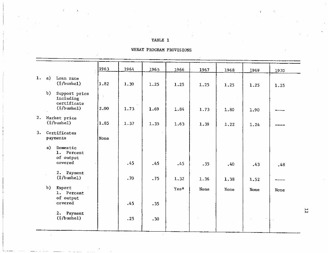
TABLE 1

WHEAT PROGRAM PROVIS IONS

1963 1964 1965 1966 1967 1968 1969 1970

1. a) Loan rate($/bushe1) 1.82 1.30 1.25 1.25 1.25 1.25 1.25 1.25

b) Support priceincludingcertificate($/bushe1) 2.00 1. 73 1.69 1.84 1. 73 1.80 1.90 ----

2. Market price($/bushe1) 1.85 1.37 1.35 1.63 1.39 1.22 1.24 ----

3. Certificatespayments None

a) Domestic1. Percentof outputcovered .45 .45 .45 .35 .40 .43 .48

2. Payment($/bushe1) .70 .75 1.32 1.36 1.38 1.52 ----

b) Export Yes* None None None None1. Percentof outputcovered .45 .35

2. Payment($/bushe1) .25 .30

.....N

TABLE 1 (Continued)

'c

1963 1964 1965 1966 1967 1968 1969 1970

4. Required conserva-tion acreage aspercent of allot-ment None 11.11 11.11 15 0 0 15 30.3

5. Additionalvoluntaryconservationacreage None None None

a) Limits 1964 1965 1966 1969 1970to larger to 15 to larger 50% of to 19.2of 15 acres of 15 allotmen1 acres oracres or or acres or 50% of20% of between 21. 7% of allotmentallotment 10 and allotment

20% ofallotment

b) Payment(percent ofline 2) 20 50 40 0 0 50 50

6. National allotment(million acres)

a) Announced 55 49.5 49.5 47.8 68.2 59.3 51.6 45.5

b) Effective 55 53.2** 53** 51.7** 68.2 59.3 51.6 45.5

t-'I.U

::l

TABLE 1 (Continued)

1963 1964 1965 1966 1967 1968 1969 1970

7. National wheatacreage (millionacres)

a) Planted 53.4 55.67 57.36 54.38 67.79 62.59 54.3 49.0

b) Harvested 45.5 49.76 49.56 49.86 58.77 55.31 47.57 43.6

8. Participation

a) Percent ofwheat farms 24 34 48 48 45 47 57 56

b) Enrolled farmersacreage as apercent ofeffectivenationalwheatallotment 46 74 82 82 84 84 82 89

Sources: Lines (1)-(7) USDA,ASCS, "Commodity Program Fact Sheets," (1963-1970). Annual generalexplanations prepared for ASCS committeemen.

Lines Sa and Sb. Letter from K. Hoover, Director of Wisconsin's ASCS office.

* ,No payment rate was established. Growers got a share of exporters' contributions and the pool basedon the size of their allotment.

**The effective allotment exceeded the nationally announced allotments because the allotments tosma11-sac1e growers were raised during these years.

~---- ---.

I-'~

15

output need not equal actual, these certificates represent a form of

insurance against crop failure. In 1964 the domestic marketing-certificates

covered 45 percent of "expected" production and paid $0.70 per bushel.

This payment is received by the grower regardless of the buyer of his output.

By 1969, this payment had risen to $1.52 per bushel for 43 percent of the

expected output.

When first introduced for 1964 the domestic marketing-certificate was

accompanied by an export marketing-certificate. This certificate in 1964

paid $0.25 per bushel for 45 percent of the calculated "expected" output

of wheat. This payment was paid almost directly to farmers by commercial

exporters and in essence represented the amount by which U.S. wheat prices

would have been below world levels. After 1966 this device was abandoned

because U.s. export prices including transport have since approached and,

at times, exceeded world levels.

The domestic marketing-certificate when first introduced was virtually

a direct payment to farmers from processors of food for domestic use. Food

processors were thereafter required to purchase a certificate for about $0.70

per bushel for all wheat used for domestic food purposes. The fund into which

these payments were made was distributed among participating growers. .Since

1966 the payment rate has been increased to the difference between parity

and $1.25 (this difference is currently about $1.30 to $1.60) of which $0.75

has been paid by processors and the remainder by the government out of eee

appropriations.

During all of the period 1964-69 the market-price per bushel was above

or within $0.03 of the loan rate. This contrasts with earlier periods when

the loan rate was above the market price; during the 1950s the market price

rose above the loan rate but once and then by $0.01 per bushel. Because theI

16

market price was above the loan level during much of the period 1964-69 the

government purchased little wheat and was able to reduce its stocks, in

part through PL 480. The relatively high ...market-price can be attributed

to the effect of the wheat commodity program and in part the high expert

level.

In particular, two measures originated after 1963 probably contributed

to the success of the Freeman programs. (1) The high value of marketing

certificates drew farmers into the program and worked in the direction of

keeping actual planting near the national allotment. (2) Payments were

offered to program participants to divert voluntarily some part of their

acreage from wheat to conservation use. This second measure is elaborated

below.

In 1964 a grower could divert the greater of 15 acres or 20 percent of

his allotment and receive 20 percent of his expected (determined as described

above) gross income from wheat from the diverted acres. For 1970 the grower

could receive 50 percent of his expected gross from diverted land up to the

larger of 50 percent of his a1loted acreage or 19.2 acres. This option

provided the opportunity to·not plant wheat on the relatively less profitable

acreage.

Thus the general effort behind the wheat program of recent years has

been directed toward raising prices through reduced production. Plantings

have been discouraged by providing economic incentives to eligible producers

to participate in the programs. Production by participating growers has

been further reduced through voluntary diversion provisions. Also, production

by nonparticipants would seem to have been curtailed. Since certificates,

as opposed t.o price, came to he the mechanism of assuring equitable incomes

17

to participants, the loan levels have come to be relatively low (the

average level between 1964-70 was about 60 percent of the level of the

1950s). Consequently, government purchases didn't act as a magnet in

raising the market price to the high support level, and lower prices should

have discouraged nonparticipants' production. The program since 1964 seems

to have been effective in reducing output and government stocks.

Participation in the program has been raised from 34 percent of wheat

growers in 1964 to 56 percent in 1970. Of acreage eligible to participate

in the program 74 percent participated in 1964 and 89 percent participated

in 1970. In some ways the programs have been tailored to increase partici­

pation by small-scale growers. Circumstantial evidence can be brought to

bear on this. Between 1964 and 1970 the farms participating increased 65

percent while acreage of participants rose by only 20 percent. This would

seem to indicate that the program has been successful in attracting small­

scale growers.

There are other relatively minor provisions in the program and these can

be found in the annual Agricultural Stabilization and Commodity Service

(ASCS) brochures.

EFFECTS OF SUPPLY CONTROL

Supply control as currently practiced does produce the desired effect of

increasing the gross incomes to participating growers both through higher

prices and direct payments. The higher market-price for output of supported

crops results from the impact of supply control. It has been noted that the

demands for major foodstuffs are inelastic. This means that the smaller

the total number of units reaching the market, the higher the price per unit.

18

Consequently, the total amount paid for all such units increases. Since

commodity programs have tended to restrict aggregate output below that

level which the growers under a free market would produce, they have

resulted in a higher gross-income from the sale of output. This increase

in gross income is supplemented with direct payments.

The objective is, of course, not only to raise gross incomes; the

success of farm programs must be judged from their impact on the profitability

of the farm operation. Such a criterion raises indirectly one of the critical

questions of farm programs. It might appear obvious that higher farm prices

and direct payments should lead to higher annual net farm-incomes to partici-

pating farms. However, many contend, following the reasoning of orthodox

economic theory, that the nature of supply control-programs leads to farm

profits being supplemented to a considerably smaller degree than gross incomes.

This result can be demonstrated for both the effects of direct payments

and higher-than-free-market prices. Since it is easier to demonstrate.how

direct payments need not necessarily result in higher net incomes to partici-

pating farmers, it is that case which is explored here.

For commodity programs to lead to higher net farm-profits requires that

production costs rise less than gross income. Let

GY -C = NP.where GY = annual gross income

C = annual costsNP = annual farm profit

If both gross income and costs were to rise by the same-amount there would be

no change in profit. (Profit is presently used in an economic opposed to a

legal sense. Profit, specifically, is net income, conventionally defined,

less the opportunity-cost of owned resources.) If gross income increases,

say through direct payments, then this would be translated fully into a

19

rise in profits only if costs remained constant. Included in costs are

both the actual and opportunity-costs of production. Actual costs includeil.,;

expenditures on seed, fertilizer, nondurable equipment an4/'other similarI

inputs. Opportunity-costs include the income foregone, for example, by

the owner's spending his labor on the farm instead of in off-farm employ~

mente Another opportunity-cost is the return on his capital which a farmer

foregoes by investing it in his operation instead of in stocks, bonds, or

other interest bearing assets. This latter opportunity-cost is of particular

importance in the subsequent argument. So long as NP is greater than or

equal to zero, the grower is doing at least as well by investing his time and

capital in his operation as he could do by allocating his resources elsewhere.

The theory which underlies the above observations on the potentially

small impact of direct payments on farm profit is illustrated by the following

example. Consider a landowner-farmer who operates one acre of land valued

at. $400. Assume that ordinarily this grower grosses $100 and earns (net of

all imputations to his labor as well as other input .costs) $20 from this

acre. Further assume that in advance of crop year 1969, the grower is told

by his USDA county committee that in crop year 1969 and forever thereafter

he will receive $10 (current dollars) per year in direct payments on this

acre. (Actually it could be assumed for added realism that he would earn

$15 in direct payments in return for performing certain tasks which would

cost, perhaps in the value of his expenditure of time, $5.)

This grower receives the benefits on the acre because he possesses title

to the land at the time the program is implemented. The benefits he receives

are not diminished if he rents the land to another farmer of if he sells it

outright.

--- - ---- ----------------------- -

20

The program represents a perpetuity. The annual direct payments of

$10 when capitalized over all time at a constant interest rate of, say,

5 percent represent a present value of $200. That is, the value of the

land increases by $200 after the program is announced. The fact that the

payment takes the form of $10 this year and $10 next year and so on is not

important. The $10 in 1969 is worth $10 to the grower. Likewise, the $10

payment in 1970 is worth $10 divided by 1.05, about $9.50, to the grower

in 1969. ($9.50 represents the amount which if invested today at 5 percent

would become $10 in a year.) The $10 payment in 1971 is worth $10 divided

2by 1.05 in 1969, and so on. The landowner is benefited in the same way either

if the program involves an outright one-time-on1y gift of $200 or if he can

receive $10 annually forever. In the latter case he can capitalize on the $200

gift by selling his land at any time for $200 more than he otherwise could have.

In this example, then, the effect of the program can be seen as raising

the price of land by $200, from $400 to $600. The benefits for all time are

realized by the person who is titleholder to the land at the time of the

program's inception. What then of a grower who purchases the land from this

original landholder? He will receive no benefits from the program if it is

continued at an unchanged level. Although he will receive $10 annually in

direct payments, thus raising his gross by $10, his costs rise by a like

amount and consequently on net he would be unaffected by the program. The

$10 rise in annual operating costs consists of the opportunity-cost of

capital. To purchase the land he must pay $200 more than he otherwise would

. have; the opportunity-cost of this, i.e., the income foregone by not

investing this elsewhere at the interest rate of 5 percent, is just $10.

21

Likewise a nonlandowning renter receives no benefits from the program.l

Assuming a perfect rental market in land, renters' bids for the allotment

land would exceed by $10 the amount they would pay for similar land not

covered by the farm program. Any year the farmer in the above example chose. ;.

to rent out the acre he would still receive the benefit payment; the form

would be higher rents as opposed to a check from the Treasury.

Theory, then, predicts that farm-program benefits will be capitalized

into higher land values and realized by the landholders of record at the

time the program begun. Reality may appear to contradict this theory for

a number of reasons.

(1) Buyers or sellers of land may feel insecure about the durationand payment levels of the farm programs. Thus, land pricesmay not rise by the full capitalized value.

(2) Markets may not be perfect; rents or the sale price of landmight be constrained by tradition and consequently might notrise by the full amount anticipated.

Clearly, the implementation of commodity programs has been accompanied.'.

by considerable uncertainty. These programs have involved experimentation

with a variety of methods of operation: for example, large purchases of

output by the CCC in the1950s and.high direct payments in the 1960s. Addition­

ally, legislation governing these programs has to be enacted regularly, and

in some cases farmers' referenda are required for the program's operation.

To this uncertainty is added lack of foreknowledge of payment levels in

future years.

All of this prevents the complete capitalization of program benefits

into land values. Thus, later generations of farm owners have received

and will continue to receive some farm-program benefits. Nonetheless, any

rise in land values will diminish the benefits of farm programs reaching

22

those purchasing land after the capitalization process has occured. Noted

below is a study which has examined the relation between the benefits of

farm programs and the value of agricultural acreage.

17Drawing from work by Bruce Johnson t Charles Schultze has noted that

the benefits of farm programs have indeed been capitalized into land values. 18

He argues that the benefits of farm programs have been added as a residual

to returns to land and the increase in this figure since the inception of

this program has paralleled the increase in land values (see Table 2). He

notes that the high program benefits of the 1960s coupled with increasing

optimism about the continuation of these programs somewhat accelerated the

capitalization process. Schultze said of this result t "The first-generation

owners capture the benefits when they sell. Second-generation owners lose

many of the benefits to higher carrying charges." Note that this result is

verified in line three of Table 2: the large increase in net returns to land t

444 percent t just about equals the 420 percent rise in land values from 1935

to 1967.

TABLE 2

CHANGE IN LAND VALUE OVER TIME

(Percentage increases per acre)

Perio.d Increase in net Increase in net Increase in landfarm income return to land values

1938-39 to 1952-54 160 124 160

1952-54 to 1965-67 18 143 100

1935-39 to 1965-67 206 444 420

Source: Schultze t The Distribution of Farm Subsidies t (1971)t p. 35.

,0

23

Later in this paper it will be shown that approximately three-fourths

of the benefits of farm programs in 1969 are attributable to direct payments.

The remaining fraction results from the higher farm prices produced by

commodity programs compared to those resulting from an otherwise free

market. These benefits, too, are capitalized in part into land values since

they are included in the residual returns to land upon which the capitalization,

reported above, takes place.

DISTRIBUTION OF FARM-PROGRAM BENEFITS

The present paper reports on a study of the distribution of farm-program

benefits for 1969. The benefits of farm programs are defined as the excess

of actual gross farm income over hypothetical long-run free-market gross

farm income. The benefits of farm programs are composed of both elements:

the higher market prices prevailing because of the effects of supply control

and direct payments for participation.

The seven crops upon which the analysis is based are feedgrains (corn,

oats, grain sorghum and barley), wheat, soybeans and cotton. These crops

constitute a substantial portion of the cash-crop sector of the economy. Of

the nearly 300 million acres harvested in 1969 these crops accounted for

abou~ 205 million acres. Of the gross cash receipts from crops (not including

direct payments) for 1969 of $22 billion, these seven crops accounted for

about $12.5 billion. Additionally, in 1969 these crops accounted for' over

$3.3 billion ,(88 percent) of the total $3.75 billion in direct government

payments to farmers.

24

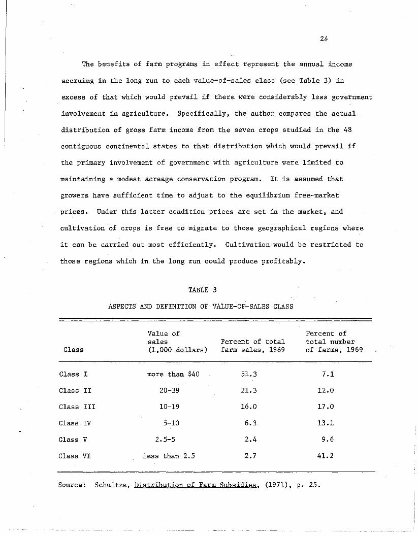
The benefits of farm programs in effect represent the annual income

accruing in the long run to each value-of-sales class (see Table 3) in

excess of that which would prevail if there were considerably less government

involvement in agriculture. Specifically, the author compares the actual·

distribution of gross farm income from the seven crops studied in the 48

contiguous continental states to that distribution which would prevail if

the primary involvement of government with agriculture were limited to

maintaini~g a modest acreage conservation program. It is assumed that

growers have sufficient time to adjust to the equilibrium free-market

prices. Under this latter condition prices are set in the market, and

cultivation of crops is free to migrate to those geographical regions where

it can be carried out most efficiently. Cultivation would be restricted to

those regions which in the long run could produce profitably.

TABLE 3

ASPECTS AND DEFINITION OF VALUE-OF-SALES CLASS

Value of Percent ofsales Percent of total total number

Class (1,000 dollars) farm sales, 1969 of farms, 1969

Class I more than $40 51.3 7.1

Class II 20-39 21.3 12.0

Class III 10-19 16.0 17.0

Class IV 5-10 6.3 13.1

Class V 2.5-5 2.4 9.6

Class VI less than 2.5 2.7 41.2

Source: Schultze, Distribution of Farm Subsidies, (1971), p. 25.

25

Note: "Class VI includes a number of categories that the Bureau of th~

Census shows separately (small commercial farms, part-time farms,etc.), with one very minor exception, these categories all havethe common characteristic of selling less than $2,500 farmproducts eacp year." Schultze, The Distribution of Farm Subsidies,p. 25.

Price-support benefits: The distribution of gross far~income from

the sale of crops among the sales classes was calculated for 1969. This

distribution was calculated assuming that the relative distribution of

acreage among sales classes reported for each state for each crop in the

1964 Census of Agriculture also prevailed in 1969. (This assumption was

required since the results of the 1969 Census were unavailable at the time

this research was performed.) The fraction of total acreage harvested for

each class for each of the crops studied in each continental state was

multiplied by the gross value of the sale of each crop in each state to

determine the share of sales attributable to each class. Summing these

quantities across all crops and all 48 continental states provided the

distribution of actual gross sales in 1969.

Obtaining the free-market distribution of gross income from the sale

of crops required the use of a model capable of generating a free-market

distribution of output. For this the Iowa State University (ISU) general

equilibrium linear programming model was used.

The spatial linear programming model in use at Iowa State's Center for

Agricultural and Economic Development is a versatile tool. It is being

used to study such matters as the impact of eliminating chemical fertilizers

and the impact of water-resource:projects on American agriculture. It

has, in the past, been used to study the impact of changes in farm legislation

t 'h d 1 . 1 d' f 19on ou put 1n t e near an re at1ve y 1stant uture.

26

In conjunction with a demand model, the programming model permits one

to determine the spatial distribution of output among producing regions

under the assumption that long-run equilibrium prevails. The long-run

equilibrium condition requires that no region produce any of the crops

(feedgrains, wheat, soybeans, and cotton) covered by the model at a loss~

The model can provide both the equilibrium prices which prevail in 1969

under the free-market conditions specified as well as the most efficient

distribution of output among producing regions. Alternatively, using a

different formulation of the model, one can specify a set of input prices and

various constraints in determining the optimal distribution of output.

This paper reports results based on the latter formulation. The input

prices used, however, approximate the free-market levels calculated by other

researchers using the ISU mode1.20

The long-run levels of free-market prices

for crops were calculated to be:

Soybeans

Wheat

Feedgrains

Cotton

$1.85 per bushel

$1.06 per bushel

$0.85 per bushel (average)

$0.22 per pound

Output from the ISU model provided information on the distribution of

output among states. It is assumed by the author that for each crop, the

distribution of output among sales classes prevailing within a state in 1964

continued to 1969 and that distribution of planting among classes would also

have prevailed under a free market in 1969. The free-market distribution

among sales classes was calculated employing the same methodology described

for the distribution of actual gross income from the sale of the seven crops.

The difference between the actual and hypothetical gross incomes from the

27

sale of the crops provides a measure of the price-support benefits of·

farm programs. Such distribution among sales classes have been calculated

by others, the most notable work having been done by Charles Schultze.

The present work reported has two primary advantages: (1) The model employed

is spatial, and consequently permits an optimal allocation of cultivation

among states. This affects the results of the distribution of farm income,

since the economic classes produce differang shares of output of the seven

crops in different states. (2) The present work calculates a distribution

of price-support benefits assuming long-run equilibrium. The long-run

formulation is .superior if one is interested in knowing how actual 1969

farm income compares with the hypothetical distribution--assuming programs

were terminated sufficiently in advance of that year to leave in production

only those areas for which production of each crop is at zero or positive

profits.

In Table 4 the results of the calculations on the price-support benefits

of farm programs are presented. These benefits are calculated for each

class as the difference between actual and free-market 1969 farm income.

TABLE 4

DISTRIBUTION OF PRICE SUPPORT BENEFITS ATTRIBUTABLE TOFEEDGRAINS, WHEAT, SOYBEANS AND COTTON IN 1969

($ million)

Va1ue-of-sa1es class

I II III IV V VI Total

1. Gross benefit 600 250 250 170 110 100 1,480

2. Actual gross fromincluded crops 2,930 3,970 3,410 2,030 830 570 12,840

3. Benefits as apercent of gross 20 8 7 8 13 18 12

Sources: Lines (1)-(2) Output of Iowa State University Model.Line (3) Farm Income Situation, 1969.

28

The above table cannot give a complete picture of the impact of farm

programs on the sale of crops since nowhere above are cost estimates included.

However, the ISU model predicts that under long-run equilibrium conditions,

21free-market production costs would about equal current actual costs.

Additionally, analysis underlying the work in this report indicates that'

output shares of the crops studied would shift only a little among economic

classes with the end of price supports. It can thus be assumed that costs

to each economic class will be approximately unchanged. This enables the

assumption that the calculated changes in gross income can be fully

translated into equal changes in net income.

This report looks only at the price-support benefits of the seven

major crops. For further analysis, it is assumed that the price-support

benefits attributable to other crops are negligible. This assumption is

necessitated because of the limited coverage of the ISU model. However,it

is justified because of the minimal controls over, and/or the relative

unimportance of, other crops. Price-support benefits are not calculated

for the following: sugar, wool and mohair, tobacco, rice, and other relatively

minor crops.

Note that the price-support benefits represent the lower bound of the

costs of farm programs to the public in their roles as consumer. The $1.48

billion represents the higher price middlemen must pay farmers for commodities

because of supply control. The cost borne by consumers will exceed this

amount if the intermediaries pursue a mark-up policy in setting their prices.

Direct payment benefits: Direct payments of slightly under $3.8 billion

were distributed to all farms in 1969. The USDA has broken down total benefit

22payments among value-of-sales classes. Of those seven crops presently

considered, only soybeans and oats did not have direct payments associated

29

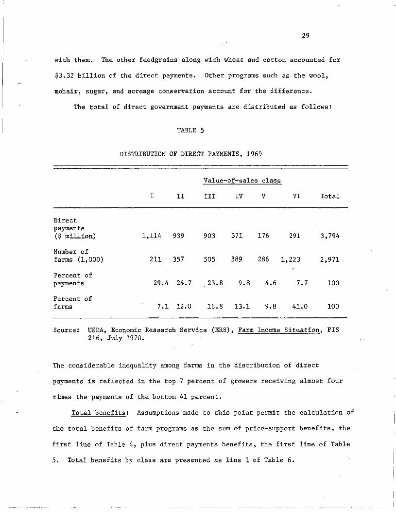
with them. The other feedgrains along with wheat and cotton accounted for

$3.32 billion of the direct payments. Other programs such as the wool,

mohair, sugar, and acreage conservation account for the difference.

The total of direct government payments are distributed as follows:

TABLE 5

DISTRIBUTION OF DIRECT PAYMENTS, 1969

Value-of-sales class

I II III IV V VI Total

Directpayments($ million) 1,114 939 903 371 176 291 3,794

Number offarms (1,000) 211 357 505 389 286 1,223 2,971

Percent ofpayments 29.4 24.7 23.8 9.8 4.6 7.7 100

Percent offarms 7.1 12.0 16.8 13.1 9.8 41.0 100

Source: USDA, Economic Research Service (ERS), Farm Income Situation, FIS216, July 1970.

The considerable inequality among farms in .the distribution of direct

payments is reflected in the top 7 percent of growers receiving almost four

times the payments of the bottom 41 percent.

Total benefits: Assumptions made to this point permit the calculation of

the total benefits of farm programs as the sum of price-support benefits, the

first line of Table 4, plus direct payments benefits, the first line of Table

5. Total benefits by class are presented as line 1 of Table 6.

30

Long-run total benefits of farm programs add up to $5.27 billion (line 1).

Of this amount about 1/3 accrues to class I and about 3/4 to classes I-III

taken together. Class VI derives 7 percent of the total benefits (line 3).

Compared to their shares of gross farm income, classes II-VI all derive' a

higher percentage share of benefits (lines 5 and 3). That the low-gross

growers derive relatively higher benefits as a percentage of. gross farm­

income is also illustrated in line 8. Here it is shown that for class VI,

benefits represent about 1/7 of gross income and for class V, about 1/5,

while for classes II and I, benefits represent but 1/10 and 1/16 respectively.

There appears to be a relatively greater supplement to the incomes of the

lower-gross farms in a comparison between benefits and gross income. However,

this progressivity largely vanishes when one compares benefits to realize

net farm-income (line 9). Such a comparison shows that farm programs supplement

net income of the sales classes fairly uniformly. All but one class would

experience about a 1/3 decline in net farm-income with the termination of·

commodity programs; the sole exception is class V--which would experience a

decline of about 1/2. The relative differences among classes between the

ratios of benefits to gross versus benefits to net farm-income, results from

the lower margins of the higher sales-class farms (line 10).

Total benefits per farm are another aspect of the equity of farm programs.

Table 6 shows that the benefits to class I farms average more than $8,000

while those to class VI but $320 (line 12) ~ The benefits per farm decline

uniformly moving from class I to class VI.

A considerable portion of farm operators derive some off-farm income.

Line 19 indicates how much accrues on average to farms by value-of-sales

class. The highest average off-farm income accrues to class VI growers.

This can be attributed largely to the fact that about 3/4 of the farms in

TABLE 6

IMPACT OF AGRICULTURAL PROGRAMS, 1969

Value-of-Sales Class

Item I II III IV V VI Total

(1) Total benefits* 1,710 1,190 1,150 540 290 390 5,270

(2) Direct payment benefitsas a percent of total 65 79 78 68 62 74 72

(3) Percent of benefits 32 23 22 10 6 7 100

(4) Realized gross farmincome* 26,530 11,480 8,840 3,630 1,490 2,630 54,600

(5) Percent of realizedgross income 49 21 16 7 3 5 100

(6) Realized net income(including payments)* 5,800 3,740 3,270 1,410 610 1,320 16,150

(7) Percent of realizednet income 36 23 20 9 4 8 100

(8) Benefits as a percent ofrealized gross 6.4· 10 13 15 19 15 9.6

(9) Benefits as a percent of wrealized net 29 32 35 38 48 29 32 I-'

(10) Net as a percent of gross 22 32 37 39 41 50 30

.(11) Number of farms** 211 357 505 389 286 1,223 2,971

TABLE 6 (Continued)

Value-of-Sales Class

Item I II III IV V VI Total

(12) Percent of farms 7 12 17 13 10 41 100

(13) Total benefits per farm** 8.1 3.3 2.3 1.4 1.0 .32 1.77

(14) Realized gross farm incomeper farm** 125.7 32.2 17 .5 9.34 5.20 2.15 18.4

(15) Production expenses perfarm** 98.2 21. 7 11.0 5.71 3.08 1.07 12.9

(16) Realized net farm incomeper farm** 27.5 10.5 6.48 6.63 2.12 1.08 5.44

(17) Direct payments per farm** 5.3 2.6 1.8 0.95 0.62 0.24 1.28

(18) Price support and spatialbenefits per farm** 2.8 0.70 0.50 0.45 0.38 0.08 0.49

(19) Off-farm income per farm** 5.46 3.24 3.14 4.49 4.90 7.01 5.26

(20) Total money income perfarm** 33.0 13.7 9.62 8.12 7.02 8.09 10.7

(21) Benefits as a percent oftotal income 25 24 24 17 14 4 16

wN

Sources: ERS, USDA, Farm Income Situation, FIS 216, July 1970. Tables 4 and 5.

*In millions of dollars.

**In thous ands of dollars.

33

this class are not commercial, i.e., they are either part-time or part

. f 23ret~rement arms. One would suspect that for this bottom class well

over 3/4 of the off-farm earnings accrue to noncommercial farms. The lumping

together of commercial with noncommercial farms, forced by the form of the

presentation of direct payments data in the Farm Income Situation of July·

1970, obscures the reliance of low-gross commercial farms on farm income.

Combining the data on farm and off-farm income and comparing the

resulting magnitude with total benefits (line 21), demonstrates the

decreasing relative liability, moving from high to low gross farms, on

total income consequent upon the termination of farm programs. Because low-

gross farms rely to a lesser extent on farm income this liability is

correspondingly lower. This last line presents the strongest evidence

against the notion that farm programs are responsible for the continued

existence of the small and, in particular, poor farms.

One way economists examine the equality of a distribution is by means

of a Gini coefficient. A coefficient of 0 indicates a perfectly even

distribution of a quantity among a population. A coefficient of 1.00 indicates

complete inequality, i.e., one person has every unit of that which the

distribution is looking at while everyone else has nothing. For comparative

purposes, the Gini coefficients of percent distribution of family personal

income in this country in 1954 and 1956 was 0.39 and in 1962 was 0.40.24

Over all, farm programs have only a small effect on the distribution of

income within agriculture. The Gini ~oefficient of the total benefit distri-

bution indicates slightly greater equality than the actual 1969 distribution

of realized net farm-income. Subtracting for each class total annual benefits

from actual 1969 realized net farm-income results in a distribution of hypo-

thetical realized net farm-income, the Gini coefficient for which is 0.58.

34

Terminating farm programs would have the effect of worsening the distribution

of net farm-income by two points (see Table 7). Highly concentrated farm

programs improve the distribution of net farm-income only because net

farm-income is itself so highly concentrated.

TABLE 7

GINI COEFFICIENTS OF VARIOUS DISTRIBUTIONS

Distribution

Direct payments

Price support and spatial benefits

Total benefits

Realized net farm-income

Hypothetical realized net farm-income

Coefficient

0.53

0.51

0.52

0.56

0.58

Benefits and land ownership: It has been argued that much of the

benefits from direct payments and price supports have been capitalized into

land values and rents. This would imply that farm operators who have acquired

their land following the capitalization process and farm renters, would not

receive the benefits attributed to them. Even if it were true that the

benefits were fully capitalized into land values, the meaningfulness of the

results of this section would not be negated. The benefits distribution is

open to two interpretations:

(1) It tells the annual benefits to farm operators by economic class

from farm programs, assuming no gains were capitalized into land values.

(2) It tells the annual loss by economic class incurred, assuming a'

capitalization process drove up land values in the past.

35

This latter interpretation looks at the benefit distribution in the

sense of an opportunity cost. The benefits received by each class are

measured by how much higher their income is under the actual as opposed

to hypothetical situation. This calculation does not assume that current

operators are actually receiving benefits from the government programs.

It does assume that they will be worse off after the programs are terminated

since their net farmrincome, in particular the return to the land, will fall,

and this will lead to a decline in land values.

In the hypothetical example illustrating the capitalization of direct

payments benefits it was noted that a later purchase would be unaffected by

the farm programs if they were continued at constant levels. However, the

termination of farm programs would result in a loss to the later purchaser

of land of $200 or $10 per year. Thus, although a current landholder may

receive no actual benefit from the farm programs, he may lose considerably

when and if they are terminated. It is in this sense that decline in income,

which would be a consequence of the termination of farm programs, is termed

a benefit. Renters in each economic class will not be similarly affected.

However, the owners of the land which they operate will suffer a capital loss •.

Thus the benefit distribution, if properly adjusted for the economic

class of the landowner, is a good indication of the annual benefits of the

programs or, looked at alternatively, the costs o:f:termina~ing thetIl,.:.

Tenurial patterns do not appear to differ considerably among connnerc.ial

economic classes. Thel964 u.s. Census of Agriculture indicates that 75

t f h . h 1 h d h . 25percen or more 0 t e. operators ~n eac c ass a owners ~p status. .

This is not to say, however, that 3/4 of the land they farmed was owned within

the economic class since (1) owned farms could on the average be larger or

36

smaller than rented farms and (2) land rented by part owners could be

owned outside their own economic class.

Significantly, the highest rates of full ownership occur among growers

of the lowest economic classes.

If it can be assumed that owners' and nonowners' farms are approximately

equal in acreage, then it follows that growers in the bottom economic classes

realize nearly the full amount of annual benefits (or will realize nearly

the entire annual losses) which have been calculated. This statement holds

with a lesser degree of certainty to the high economic classes since full

ownership occurs with lower frequency. On the other hand it seems plausible,

though it cannot be ascertained, that ownership of land rented by part

owners and tenants, is concentrated in the higher economic classes. The

available evidence indicates that the opportunity-costs of ending farm

programs, the calculated "benefits" of farm programs, accurately reflects

the distribution among economic classes.

CONCLUSION

This paper has evaluated commodity programs in terms of their impact on

the distribution of income within agriculture. It has been shown that these

programs redistribute relatively little income to the lower tail of the

income distribution. However, few would claim that the sole, or even

central, rationale of commodity programs has been their potential usefulness

as surrogate welfare programs. Rather, the primary purpose of these programs

seems to have been to maintain farm income in the aggregate. This objective,

the paper demonstrates, has to a degree been attained by supply-control programs.

37

Nonetheless, commodity programs remain as one of the foremost

mechanisms addreseed to the rural poverty problem. The President's

National Advisory Commission on Rural Poverty said of them,

• our public programs in rural America are woefully out ofdate. Many of them, especially your farm programs and vocationalagriculture programs, are relics from an earlier era. Theywere developed during a period when there was a strong beliefthat people born in rural America should stay there and work onfarms, or in farrnrre1ated occupations. The programs emergedfrom legislation which equated the welfare of farm familieswith conditions on farms and the welfare of rural communitieswith the incomes of farmers. These conditions no longer prevail.

• • • instead of combatting low incomes among rural people, theseprograms have helped to increase the wealth of land owners whilelargely bypassing the rural poor. 26

The data presented in Tables 4, 5, and 6 demonstrate the concentration

of benefits among the farm population. The bottom 41 percent (1,223,000

farms) of the producing units, class VI, receive only 7 percent ($390 billion)

of the benefits. The bottom 63 percent (1,898,000 farms), classes IV-VI,

receive only 23 percent ($1,220 million) of the benefits. Included among. these

farms are many nonpoor operators, since the mean total money income. to

operators of class IV, V, and VI, is $8,120, $7,020, and $8,090 respectively.

27The 29 percent of the farm population which is poor receives only a small

share of the benefits of farm programs.

A rough calculation will illustrate this. Assume the poor 29 percent

constitute a like percentage of the operators and receive a proportionate

share of benefits accruing to the bottom 63 percent of operators. The benefits

of farm programs reaching this population then totals about $560 mi11ion~

This extremely liberal estimate of the benefits reaching the rural poor,

even assuming further that these benefits were not largely capitalized into

land values before the land came into the hands of the poor, is indicative

of the inadequacy of farm programs in dealing with the rural poverty. The

38

President's Commission has estimated that, "To close the income gap for

the rural poor alone would cost nearly $5 billion.,,28 It should be stressed

that closing the income gap means bringing the rural poverty population

up to the equivalent of 85 percent of the urban poverty line.

Farm programs, at the very most, contribute to closing this gap by

ten percent. The cost of doing this alone, $5.25 billion annually, exceeds

the size of the gap by a quarter billion dollars.

Charles Schultze has pointed out another fault in the present approach.

He has correctly commented that the concept of parity income is an

unattainable goal of farm policy.29 Briefly, he argues that farmers are

willing to stay in that occupation at below parity-incomes. Any attempt to

raise their incomes above this level will result in a rise in land rents

and ultimately a rise in land values. A later calculation .of parity income

will show that it has risen, because of a higher input cost, and the farmer

will appear to be little, if at all, better off in comparison between

actual and parity incomes.

The implication of his argument is that only those subsidies granted to

individuals instead of to saleable assets will not be capitalized into land

values.

This insight is both an important criticism of past programs and,

a beacon to light the way to further reforms. Future farm policy must

recognize the important limitations of supply control in influencing incomes

of the farm population. Of course, increasing the benefits of the current

type of farm programs would increase the dollar benefits reaching poor

landowning farmers. However, this approach to income maintenance is

undesirable for four reasons. First, it would still not channel income to

39

all those in need, since the mechanism is selective and bypasses tenants,

hired farm workers, and the other landless agriculturalists. Second,

it is an inefficient way of redistributing income since the bulk of the

increased benefits would accrue to the higher-income growers. Third, the

capitalization of benefits into land values remains a problem. Lastly,

supply controls tend to result in farm prices above free-market levels.

Since this is translated into higher food prices, a relatively great burden

from this rise is borne by low-income consumers, the group whose food

budget tends to be a large share of their income.

An attempt has been made to reduce the amount of farm program direct­

payment benefits accruing to the biggest growers. Currently, a grower is

limited to $50,000 in direct payments per crop. In theory, such a limitation

would offer a means to defend the current type of program from the charge

that it is "woefully out of date" and unable to deal with the problems posed

by the poor within agriculture. A limitation on individual payments would

permit increased benefit levels without the amount going to the biggest farm

growing way out of publicly acceptable bounds. Furthermore, a payments

limitation works in the direction of evening the distribution of benefits.

However, the limit of $50,000 per farmer per crop is so high that it will

have minimal impact on the over all distributional consequences of the present

type of farm program.

In the 1968 wheat program, only 41 growers received more than $50,000

indirect payments, only 8 of these more than $100,000 and only one of those

received between $500,000 and $1,000,000. 30 In 1968, for all major programs

combined, only 1,274 producing units received more than $50,000; the total

payments they received were slightly more than $100 million. 3l The vast

J _

40

bulk of the benefits, about 86 percent was received by those whose benefits

were in the range of $1,000 to $49,999. (See Table 8.) Consequently,

a uniform increase in benefits, even with a limitation would still be

accompanied by the overwhelming majority of the payments flowing to the

large-scale growers. An additional defect of payment limitations is that

most growers can effectively short circuit the limitation by splitting their

32holdings among such units as family trusts.

Future farm policy must take a considerably different course if it is

to have a meaningful impact on the poor within agriculture. It is well

beyond the scope of the present work to specify the details required of

such a policy. However, this paper has pointed out the limitations of

present policies and this should serve as a guide to what has been ineffective.

41

TABLE 8

FREQUENCY DISTRIBUTION OF PRODUCER PAYMENTS, EXCLUDING WOOLAND SUGAR, UNITED STATES, CALENDAR YEAR 1968

Producers Total Amount of PaymentsPayment Range Percent Distribution Percent Distribution

less than $100 11.9 .4

$100-499 33.8 6.9

$500-999 21.2 11.4

$1,000-4,999 28.7 44.3

$5,000-9,999 3.1 15.8

$10,000-24,999 1.1 12.6

$25,000-49,999 .2 4.8

$50,000-99,999 * 2.1

$100,000 and over * 1.6·

total percentage 100.0 100.0

total numbers 2,371,634 $3,187.3 million

Source: Unpublished Tables, ERS, USDA, (July 1, 1969).

*is less than 0.1 percent.

For example, Roman conquests in the 3rd and 2nd centuriesavailability of thousands of slaves. Slavery madeand hence the domination of Roman agriculture by th~

(,

42

FOOTNOTES

1An example is the Ptolemaic Kingdom in Egypt. Their agriculturewas so centralized that all transport of the major food crops was carriedout by the state. "Prices for the most important provisions t like bread t

were steadily balanced for more than 300 years •••• " See Fritz M.Heichelheimt An Ancient Economic History, Vol. III. (Leyden, A.W. Sijthoff,1970) t p. 89.

2Ibidq p. 160.B.C. resulted in theplantations possibleupper class.

3Karl Po1anyi t Dahomey and the Slave Trade (Seattle: Universi~y ofWashington Press, 1966), p. 90.

4Edwin Nourse, Joseph S. Davis, and John D. Black, Three Years of theAgricultural Adjustment Administration (Washington D.C.: The BrookingsInstitution, 1937), p. 23.

5See Don F. Hadwiger, Federal Wheat Commodity Programs (Ames: Iow~

State University Press, 1970), for an interesting political history of theAgricultural Adjustment Act (AAA).

6United States Department of Agriculture (USDA), Yearbook of Agriculture,1934, pp. 21, 22.

7United States Department of Agriculture (USDA), Yearbook of Agriculture,1935, 144 ff.

8Ibid ., p. 35.

9Ibid., pp. 31, 115.

10Hadwiger, Federal Wheat Commodity Programs, 137 ff.

11D• Gale Johnson has put this succinctly in "Efficiency and Welfare Con­siderations of U.S. Agricultural Policy," Journal of Farm Economics, 45, no. 2(May, 1963): 332. "The rationale for extensive governmental involvement hasbeen that the income of farm families remains below that of nonfarm families."

12See for example, The 1969 Voluntary Feed Grain and Wheat Programs,PA-906, Agricultural Stabilization and Conservation'Service, United'States Department of Agriculture, January 1969.

13See Wayne D. Rasmussen and Gladys Baker, "Programs for Agriculture1933-1965," Agricultural Economics Research, (July 1966), Economic ResearchService, United States Department of Agriculture, reprinted in Vernon Ruttonet a1., Agricultural Policy in an Affluent Society (New York: W.W. Norton,1969) pp. 69-88. Also see in this same volume F. L. Thomson and R.J. Foote,"Parity Prices," pp. 90-95.

"

l4Rutton et al., Agricultural Policy, p. 94.

15 . dSee National Advisory Commission on Foo and Fiber,Concept Needed," reprinted in Rutton et aL, Agricultural

43

"Parity: NewPolicy, pp. 96-98.

l6The 1969 Voluntary Feed Grain and Wheat Programs, p. 8.

l7Bruce B. Johnson, "An Active Land Market in Perspective," Farm RealEstate Market Developments, CD-71 (December 1968),- pp. 27-35.

18Charles Schultze, The Distribution of Farm Subsidies, (Washington, D.C.:The Brookings Institution, 1971), Chapter 4.

19See L. V. Mayer et al., "Farm Programs for the 1970s," Center forAgricultural and Economic Development Report No. 32, (Ames: Iowa StateUniversity, 1968). E. o. Heady, et aL, "Analysis of Some Farm ProgramAlternatives for the Future," Center for Agricultural and Economic DevelopmentReport No. 34, (Ames: Iowa State University, 1969). Howard Madsen, et a1.,"Trade-offs in Farm Policy," Center for Agricultural and Economic DevelopmentReport No. 36, (Ames: Iowa State University, 1970).

20See Mayer, "Farm Programs for the 1970's," p. 33.

21Ibid ., p. 34.

22United States Department of Agriculture, Economic Research Service,Farm Income Situation, (FIS 216), July 1970.

23See 1964 U.S. Census of Agriculture, Vol. II, Chapter 6, p. 599. Basedon figures for 1964.

24See Edward Budd, Inequality and Poverty (New York: . W.W. Norton, 1967),p. xii.

251964 U.S. Census of Agriculture, Vol. II, Chapter 6, p. 638.

26The People Left Behind (Washington, D.C.: U.S. Government Printing

Office, 1967), p. 13.

27Ibid ., Chapter 1, Table L

28Ibid ., p. 7.

29Charles Schultze, The Distribution of Farm Subsidies, p. 40.

30United States Department of Agriculture, Economic Research Service,unpublished tables.

3~nited States Department of Agriculture, Economic Research Service,unpublished tables (dated July 1, 1969).

32The People Left Behind, p. 145. The President's Commission recognizedthis potential drawback to a payments limitation scheme.