File Structures and

Indexing

CPS352: Database Systems

Simon Miner

Gordon College

Last Revised: 10/11/12

Agenda

• Check-in

• Database File Structures

• Indexing

• Database Design Tips

Check-in

Database File Structures

File System Performance

• Often the major factor in DBMS performance

• Response time – time between issuing a command and

seeing its results

• Want to minimize this

• Throughput – number of operations per unit of time

• Want to maximize this

• Especially important for a system with many users (i.e.

large scale web site)

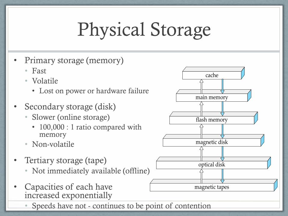
Physical Storage

cache

main memory

flash memory

magnetic disk

optical disk

magnetic tapes

• Primary storage (memory)

• Fast

• Volatile

• Lost on power or hardware failure

• Secondary storage (disk)

• Slower (online storage)

• 100,000 : 1 ratio compared with memory

• Non-volatile

• Tertiary storage (tape)

• Not immediately available (offline)

• Capacities of each have increased exponentially

• Speeds have not - continues to be point of contention

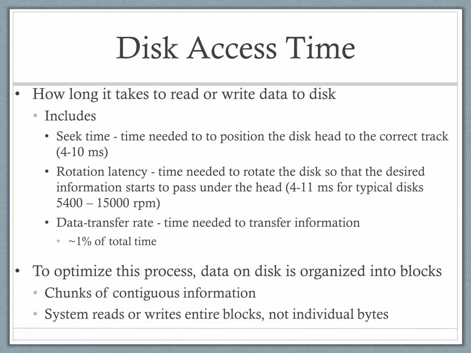
Disk Access Time

• How long it takes to read or write data to disk

• Includes

• Seek time - time needed to to position the disk head to the correct track

(4-10 ms)

• Rotation latency - time needed to rotate the disk so that the desired

information starts to pass under the head (4-11 ms for typical disks

5400 – 15000 rpm)

• Data-transfer rate - time needed to transfer information

• ~1% of total time

• To optimize this process, data on disk is organized into blocks

• Chunks of contiguous information

• System reads or writes entire blocks, not individual bytes

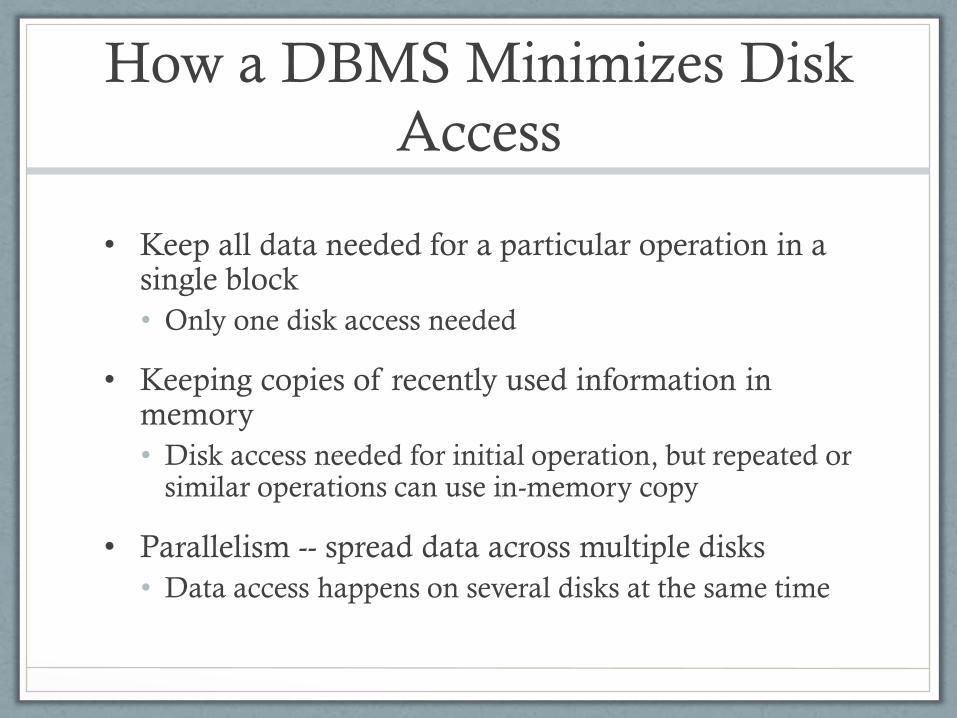
How a DBMS Minimizes Disk

Access

• Keep all data needed for a particular operation in a single block

• Only one disk access needed

• Keeping copies of recently used information in memory

• Disk access needed for initial operation, but repeated or similar operations can use in-memory copy

• Parallelism -- spread data across multiple disks

• Data access happens on several disks at the same time

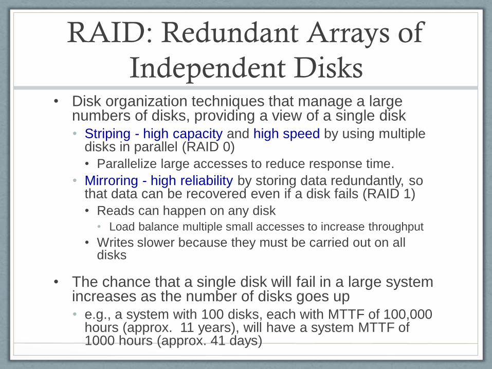
RAID: Redundant Arrays of

Independent Disks • Disk organization techniques that manage a large

numbers of disks, providing a view of a single disk • Striping - high capacity and high speed by using multiple

disks in parallel (RAID 0)

• Parallelize large accesses to reduce response time.

• Mirroring - high reliability by storing data redundantly, so that data can be recovered even if a disk fails (RAID 1)

• Reads can happen on any disk

• Load balance multiple small accesses to increase throughput

• Writes slower because they must be carried out on all disks

• The chance that a single disk will fail in a large system increases as the number of disks goes up • e.g., a system with 100 disks, each with MTTF of 100,000

hours (approx. 11 years), will have a system MTTF of 1000 hours (approx. 41 days)

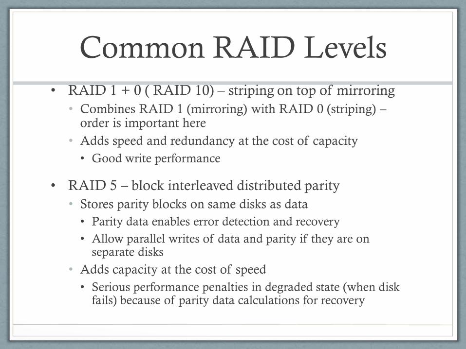
Common RAID Levels

• RAID 1 + 0 ( RAID 10) – striping on top of mirroring

• Combines RAID 1 (mirroring) with RAID 0 (striping) – order is important here

• Adds speed and redundancy at the cost of capacity

• Good write performance

• RAID 5 – block interleaved distributed parity

• Stores parity blocks on same disks as data

• Parity data enables error detection and recovery

• Allow parallel writes of data and parity if they are on separate disks

• Adds capacity at the cost of speed

• Serious performance penalties in degraded state (when disk fails) because of parity data calculations for recovery

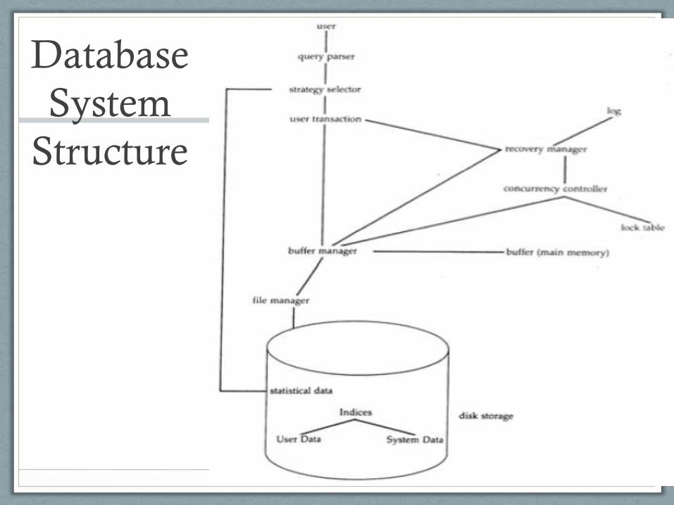
Database

System

Structure

Database System Structure:

Data Components • Database itself is stored as one or more files on disk

• As a collection of files – i.e. one for each table (MySQL)

• A single large file on the operating system in which the DBMS builds its own file system (DB2)

• Hybrid of these approaches (Oracle – tablespace files)

• Classifications of data

• User data

• Systems data

• Data dictionary or system catalog

• User access control data

• Statistical data about data access

• Index data

• Logging data

Database System Structure:

Memory Components

• Main memory buffer pools

• Stores most recently accessed block from disk for each

table (at a minimum)

• Often, retains data that has been used once and is likely

to be used again

• Logic needed to manage what data is kept in the pool

• Since memory is usually smaller than the entire database

Database System Structure:

Software Components

• Buffer manager – manages the memory pool

• Query parser -- accepts and translates queries

• Strategy selector – plans the best way to carry out queries

• Crash recovery manager – restores data to a consistent

state after an unexpected failure

• Uses a log of changes made to the database

• Concurrency controller – prevents inconsistencies from

simultaneous changes to same data by multiple users

File Organization Approaches

• Fixed-length records

• Variable-length records

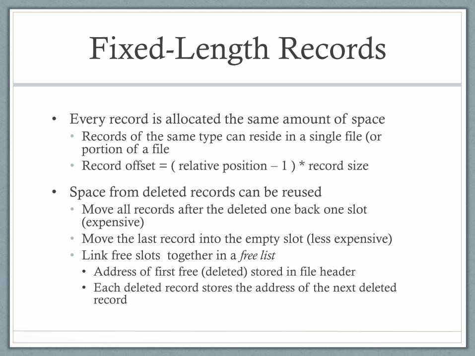
Fixed-Length Records

• Every record is allocated the same amount of space

• Records of the same type can reside in a single file (or portion of a file

• Record offset = ( relative position – 1 ) * record size

• Space from deleted records can be reused

• Move all records after the deleted one back one slot (expensive)

• Move the last record into the empty slot (less expensive)

• Link free slots together in a free list

• Address of first free (deleted) stored in file header

• Each deleted record stores the address of the next deleted record

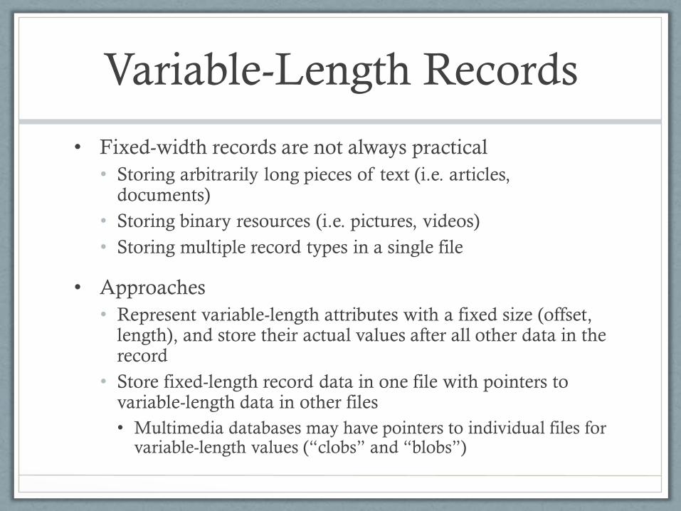
Variable-Length Records

• Fixed-width records are not always practical

• Storing arbitrarily long pieces of text (i.e. articles, documents)

• Storing binary resources (i.e. pictures, videos)

• Storing multiple record types in a single file

• Approaches

• Represent variable-length attributes with a fixed size (offset, length), and store their actual values after all other data in the record

• Store fixed-length record data in one file with pointers to variable-length data in other files

• Multimedia databases may have pointers to individual files for variable-length values (“clobs” and “blobs”)

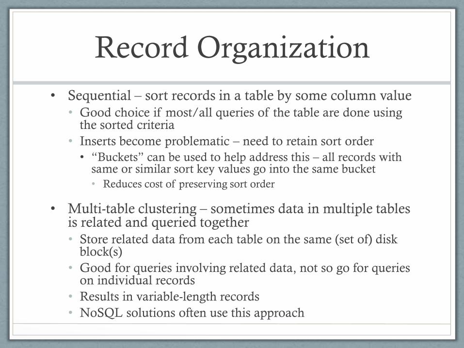
Record Organization

• Sequential – sort records in a table by some column value

• Good choice if most/all queries of the table are done using the sorted criteria

• Inserts become problematic – need to retain sort order

• “Buckets” can be used to help address this – all records with same or similar sort key values go into the same bucket

• Reduces cost of preserving sort order

• Multi-table clustering – sometimes data in multiple tables is related and queried together

• Store related data from each table on the same (set of) disk block(s)

• Good for queries involving related data, not so go for queries on individual records

• Results in variable-length records

• NoSQL solutions often use this approach

Buffer Management

• How does the DBMS decide which data is tossed from the buffer when new query results are being loaded?

• Policies

• Least Recently Used (LRU) – toss the buffer contents which have not been used for the longest period of time

• Based on the idea that past query patterns are a good predictor of the future

• Most Recently Used (MRU) – toss the buffer contents which have been used most recently

• Good when cycling through contents of a table which is too big for memory

• Based on frequency of block usage

• Examples: blocks in the data dictionary, root blocks of indexes

Indexing

Indexing Overview

• Indexes (indices) used to efficiently search for row(s) in a table that match certain criteria

• Find the disk block with the desired data with minimal disk accesses

• Index trade-off

• Improved search efficiency vs.

• Cost of maintaining the index

• Disk space required for index

• Search key

• Attribute(s) used to do lookups on an index

• Multiple indexes can be created on a table with different search keys

Index Considerations

• What will the index be used for?

• Find rows which match exact values

• Range queries (i.e. values between, greater, or less than some bounds)

• Sequential access of all rows in the table

• How frequently is the underlying data modified?

• Lots of inserts, updates, and deletes mean more index maintenance

• Read-only / read-mostly data can use indexes that facilitate faster data access but are expensive to maintain

• Is the search key a superkey (or the primary key)?

• Can multiple rows share a single key value?

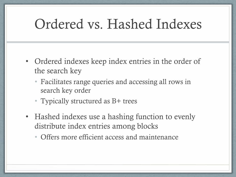
Ordered vs. Hashed Indexes

• Ordered indexes keep index entries in the order of

the search key

• Facilitates range queries and accessing all rows in

search key order

• Typically structured as B+ trees

• Hashed indexes use a hashing function to evenly

distribute index entries among blocks

• Offers more efficient access and maintenance

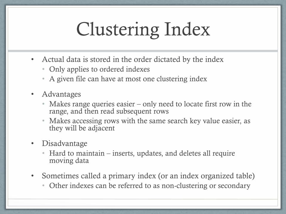
Clustering Index

• Actual data is stored in the order dictated by the index

• Only applies to ordered indexes

• A given file can have at most one clustering index

• Advantages

• Makes range queries easier – only need to locate first row in the range, and then read subsequent rows

• Makes accessing rows with the same search key value easier, as they will be adjacent

• Disadvantage

• Hard to maintain – inserts, updates, and deletes all require moving data

• Sometimes called a primary index (or an index organized table)

• Other indexes can be referred to as non-clustering or secondary

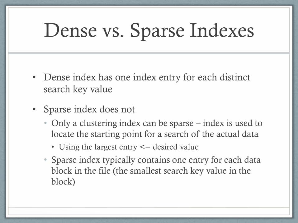
Dense vs. Sparse Indexes

• Dense index has one index entry for each distinct

search key value

• Sparse index does not

• Only a clustering index can be sparse – index is used to

locate the starting point for a search of the actual data

• Using the largest entry <= desired value

• Sparse index typically contains one entry for each data

block in the file (the smallest search key value in the

block)

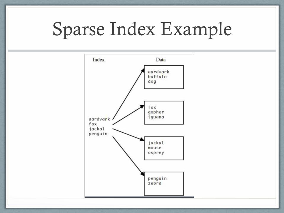
Sparse Index Example

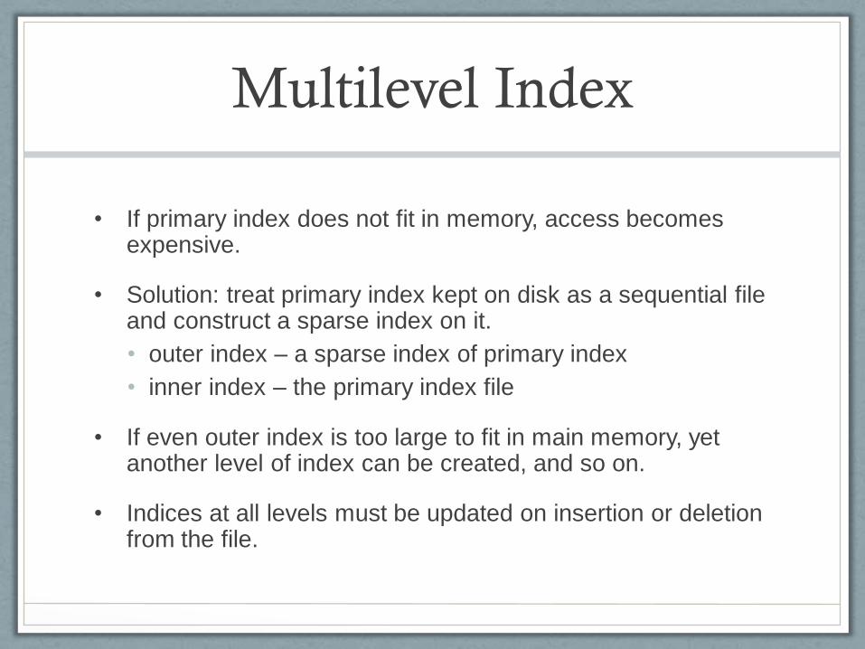
Multilevel Index

• If primary index does not fit in memory, access becomes expensive.

• Solution: treat primary index kept on disk as a sequential file and construct a sparse index on it.

• outer index – a sparse index of primary index

• inner index – the primary index file

• If even outer index is too large to fit in main memory, yet another level of index can be created, and so on.

• Indices at all levels must be updated on insertion or deletion from the file.

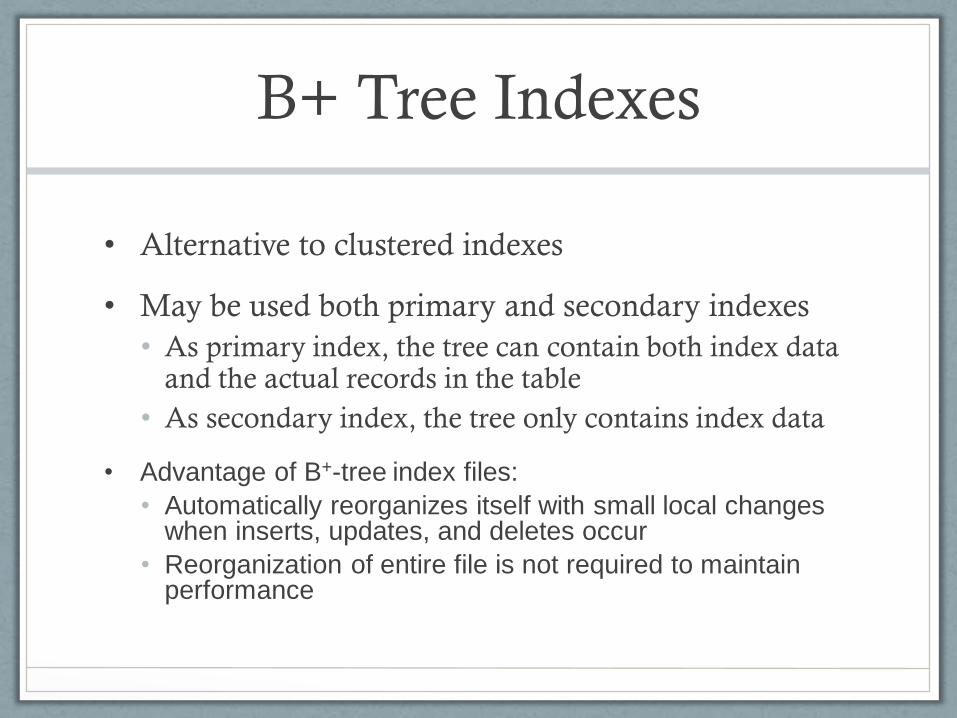
B+ Tree Indexes

• Alternative to clustered indexes

• May be used both primary and secondary indexes

• As primary index, the tree can contain both index data and the actual records in the table

• As secondary index, the tree only contains index data

• Advantage of B+-tree index files:

• Automatically reorganizes itself with small local changes when inserts, updates, and deletes occur

• Reorganization of entire file is not required to maintain performance

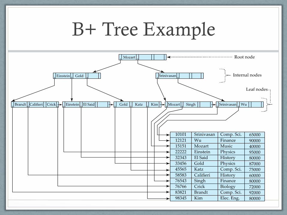
B+ Tree Example

B+ Tree Structure

• Multi-leveled with all leaf nodes on the same

level

• The order (n) of a B+ tree is determined by the

size of a node and the size of a key-value pair

• Components

• Root (with at least 2 children)

• Internal (non-leaf) nodes

• Leaf nodes

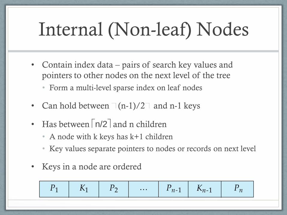
Internal (Non-leaf) Nodes

• Contain index data – pairs of search key values and

pointers to other nodes on the next level of the tree

• Form a multi-level sparse index on leaf nodes

• Can hold between (n-1)/2 and n-1 keys

• Has between n/2 and n children

• A node with k keys has k+1 children

• Key values separate pointers to nodes or records on next level

• Keys in a node are ordered

Leaf Nodes

• Comprised of one of the following

• Index data -- pairs of search key values with pointers to actual

records

• Contain between (n-1)/2 and n-1 search key values

• Last pointer in an indexing leaf node points to next leaf node

(instead of a record)

• Actual records

• In primary index

• Number of records in a leaf depends on the size of each record

(separate from order of the B+ tree)

• May also include pointer to next leaf

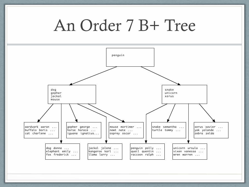
An Order 7 B+ Tree

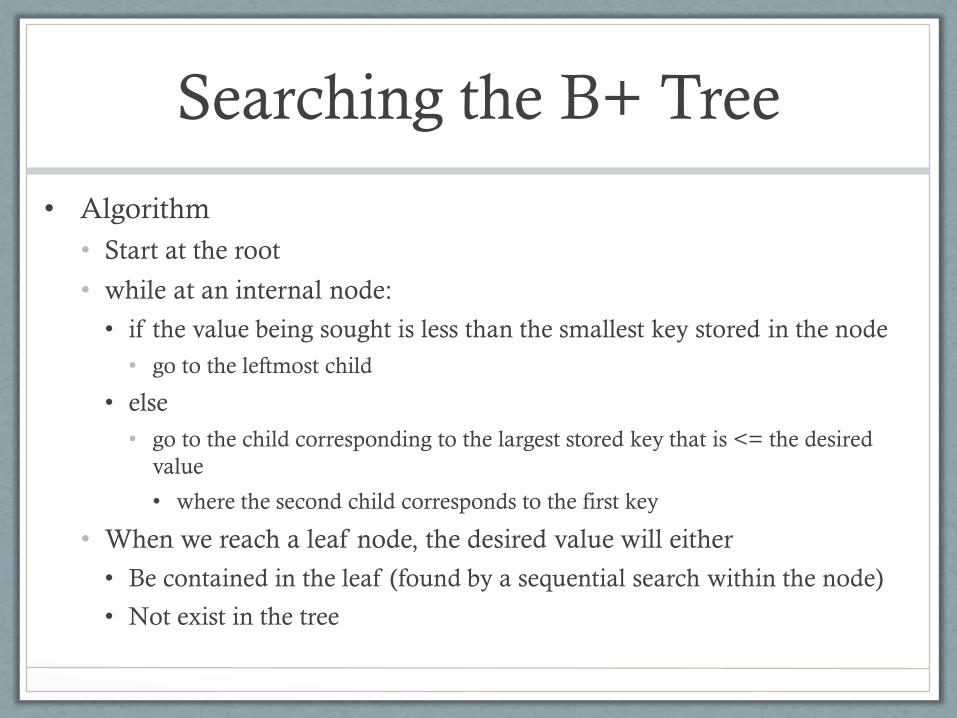
Searching the B+ Tree

• Algorithm

• Start at the root

• while at an internal node:

• if the value being sought is less than the smallest key stored in the node

• go to the leftmost child

• else

• go to the child corresponding to the largest stored key that is <= the desired

value

• where the second child corresponds to the first key

• When we reach a leaf node, the desired value will either

• Be contained in the leaf (found by a sequential search within the node)

• Not exist in the tree

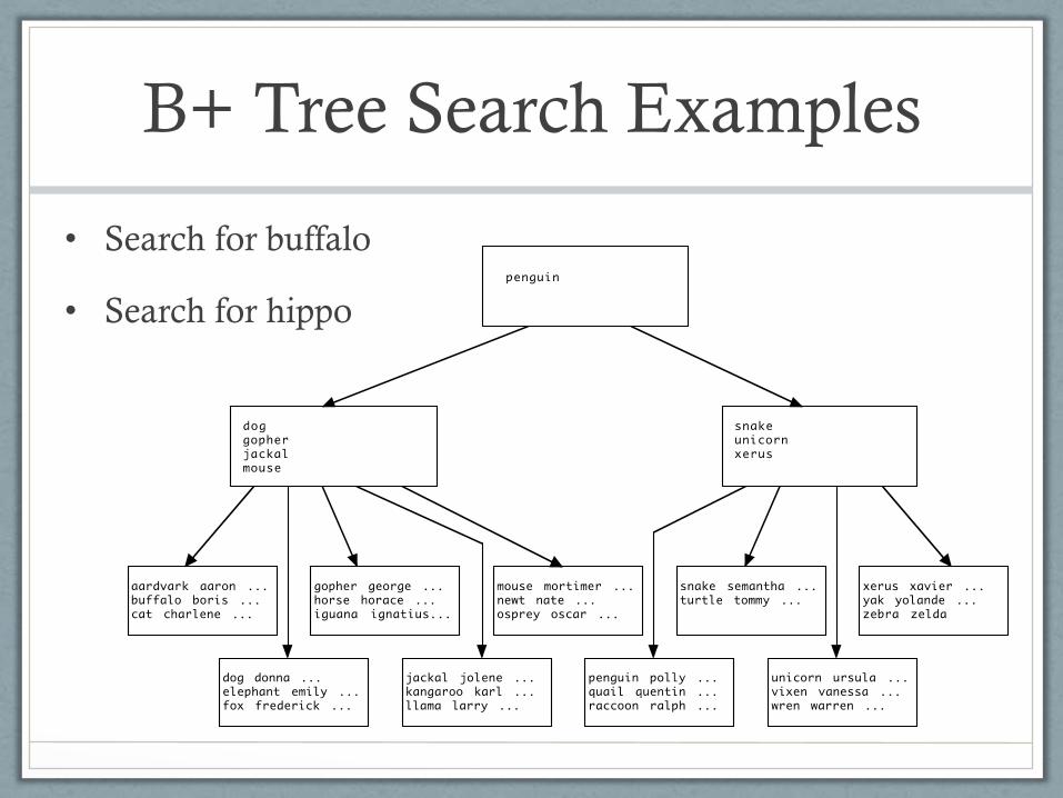
B+ Tree Search Examples

• Search for buffalo

• Search for hippo

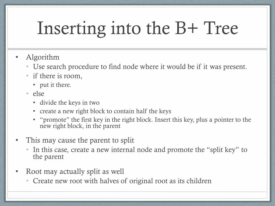
Inserting into the B+ Tree

• Algorithm

• Use search procedure to find node where it would be if it was present.

• if there is room,

• put it there.

• else

• divide the keys in two

• create a new right block to contain half the keys

• “promote” the first key in the right block. Insert this key, plus a pointer to the new right block, in the parent

• This may cause the parent to split

• In this case, create a new internal node and promote the “split key” to the parent

• Root may actually split as well

• Create new root with halves of original root as its children

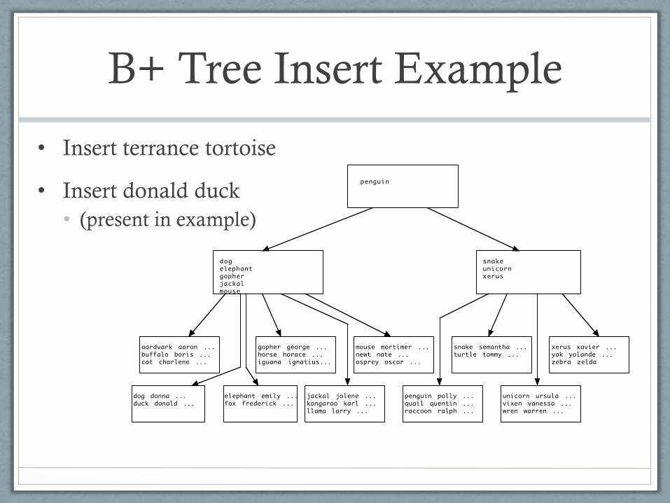
B+ Tree Insert Example

• Insert terrance tortoise

• Insert donald duck

• (present in example)

Hashing

• Alternate index structure facilitating fast access

• Search key hashed to look up records (primary index)

• Search key hashed to look up record pointers

(secondary index)

• Records (or record pointers) reside in one of several

buckets

• A hashing function on the search key determines which

bucket a record/pointer goes in

Hashing Functions

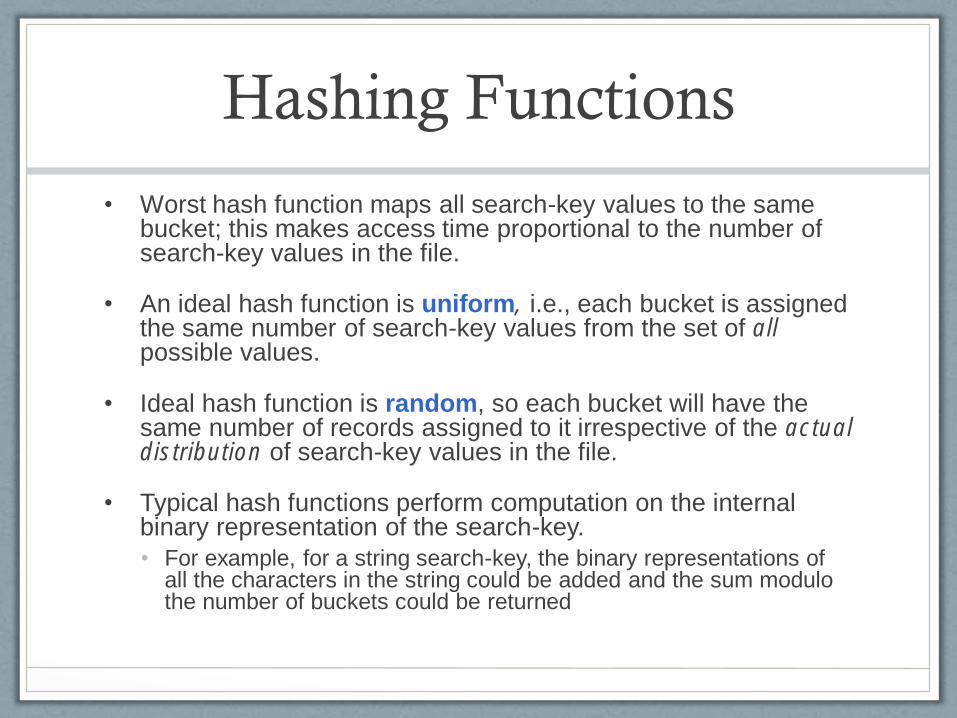
• Worst hash function maps all search-key values to the same bucket; this makes access time proportional to the number of search-key values in the file.

• An ideal hash function is uniform, i.e., each bucket is assigned the same number of search-key values from the set of all possible values.

• Ideal hash function is random, so each bucket will have the same number of records assigned to it irrespective of the actual distribution of search-key values in the file.

• Typical hash functions perform computation on the internal binary representation of the search-key.

• For example, for a string search-key, the binary representations of all the characters in the string could be added and the sum modulo the number of buckets could be returned

Hashing

Example

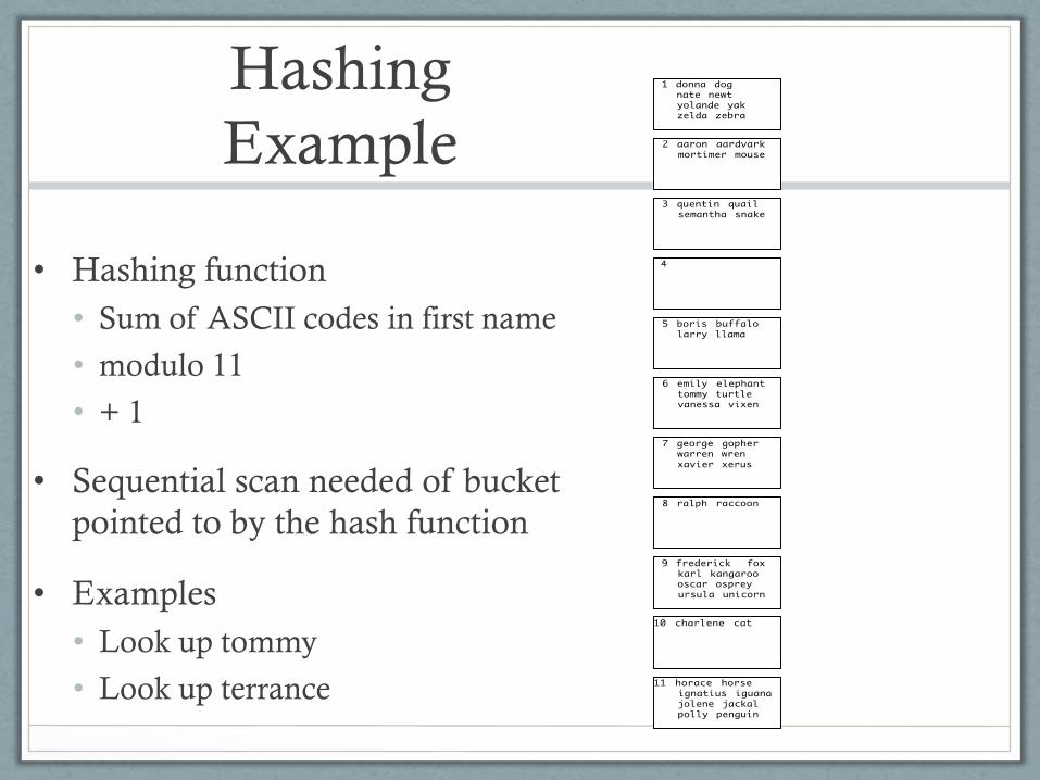
• Hashing function

• Sum of ASCII codes in first name

• modulo 11

• + 1

• Sequential scan needed of bucket

pointed to by the hash function

• Examples

• Look up tommy

• Look up terrance

Hashing Challenges

• What happens when a bucket runs out of room?

• Because of an insufficient number of buckets

• Because multiple records have the same search key (and hence, hash value)

• Because the hashing function is non-uniform

• Possibilities

• Overflow buckets

• Reorganize the file with a new hashing function

• Extendable hashing – dynamically modify the number of buckets

Comparison of Ordered and

Hashed Indexes

• Hashed indexes

• Allow fast access for exact match queries– usually 1 or 2 disk accesses (for primary and secondary indexes, respectively)

• Do not support range queries or sequential access of entire table

• Ordered Indexes

• Slower access – potentially several disk accesses as you work through the B+ tree levels

• Supports more types of queries

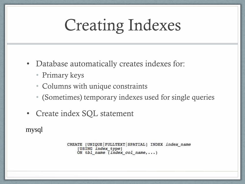
Creating Indexes

• Database automatically creates indexes for:

• Primary keys

• Columns with unique constraints

• (Sometimes) temporary indexes used for single queries

• Create index SQL statement

mysql

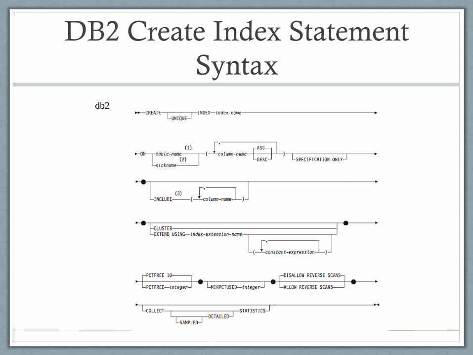
DB2 Create Index Statement

Syntax

db2

Database Design Tips

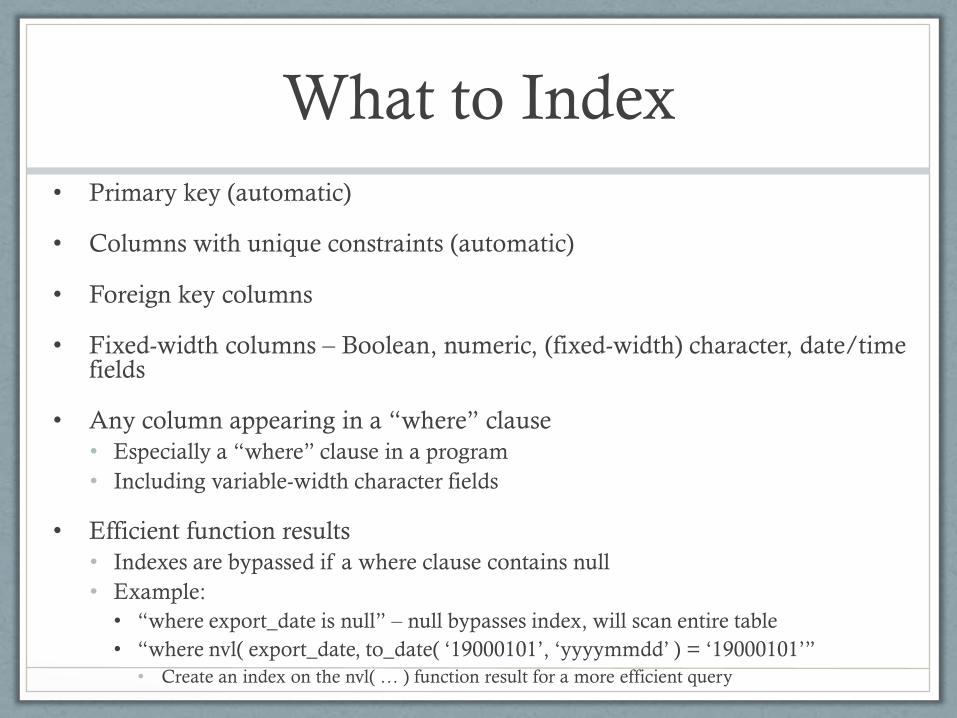
What to Index

• Primary key (automatic)

• Columns with unique constraints (automatic)

• Foreign key columns

• Fixed-width columns – Boolean, numeric, (fixed-width) character, date/time fields

• Any column appearing in a “where” clause

• Especially a “where” clause in a program

• Including variable-width character fields

• Efficient function results

• Indexes are bypassed if a where clause contains null

• Example:

• “where export_date is null” – null bypasses index, will scan entire table

• “where nvl( export_date, to_date( ‘19000101’, ‘yyyymmdd’ ) = ‘19000101’”

• Create an index on the nvl( … ) function result for a more efficient query

Don’t Index…

• Small tables (< 100 records) that will stay small

• i.e. list of states and their capitals

• Columns containing binary (blob) or large text (clob)

data

• Columns containing data that may be fetched or

updated, but will never appear in a "where” clause

• Long-ish variable width text fields (i.e. product

descriptions, review text, comments)

Index Names

• Explicitly name your indexes

• Don’t let the database make up names for you

• Index naming conventions

• Begin with 2-5 letter prefix of table name or abbreviation

• Column name(s) or abbreviation(s) that comprise the index’s search key

• End with a date stamp (i.e. 20121011)

• Gives the index a unique name

• Helpful when you need to rebuild the index or copy the table

• Prefix or suffix the following indexes

• Primary keys – “pk”

• Foreign keys – “fk”

• Unique constraints – “uniq

See you in 2 weeks!

Don’t forget to finish your design project and prepare your final

presentation on it for our next class.