Filtering and Planning in Information Spaces ∗ Steven M. LaValle Department of Computer Science University of Illinois Abstract This tutorial presents a fresh perspective on modeling sensors and then using them for filtering and planning. The concepts and tools are motivated by many problems of current interest, such as tracking, monitoring, navigation, pursuit-evasion, exploration, and mapping. First, an overview of sensors that appear in numerous systems is presented. Following this, the notion of a virtual sensor is explained, which provides a mathematical way to model numerous sensors while abstracting away their particular physical implementation. Dozens of useful models are given. In the next part, a new perspective on filtering is given based on information spaces. This includes classics such as the Kalman and Bayesian filters; however, it also opens up a new family of reduced-complexity filters that try to maintain as little information as possible while performing their required task. Finally, the planning problem is presented in terms of filters and information spaces. Contents 1 Introduction 3 2 Physical Sensors 6 2.1 What Is a Sensor? ..................................... 6 2.2 Where Might We Want to Use Sensors? ......................... 7 2.3 What Physical Quantities Are Sensable? ......................... 8 2.4 What Sensors Are Available? ............................... 8 2.5 Common Sensor Characteristics .............................. 10 3 Virtual Sensors 11 3.1 Physical State Spaces ................................... 11 3.1.1 A mobile robot among obstacles ......................... 12 3.1.2 A bunch of bodies ................................. 13 3.1.3 Fields ........................................ 14 3.1.4 Introducing Time .................................. 15 3.2 Virtual Sensor Models ................................... 15 3.2.1 The Sensor Mapping ................................ 15 3.2.2 Basic Examples ................................... 16 3.2.3 Depth Sensors ................................... 16 3.2.4 Detection Sensors ................................. 19 ∗ Technical Report, Dept. of Computer Science, University of Illinois at Urbana-Champaign, October 2009. This paper accompanied an IROS tutorial in St. Louis, USA, on 11 Oct. 2009. 1
Transcript
Filtering and Planning in Information Spaces∗
Steven M. LaValleDepartment of Computer Science
University of Illinois
Abstract
This tutorial presents a fresh perspective on modeling sensors and then using them forfiltering and planning. The concepts and tools are motivated by many problems of currentinterest, such as tracking, monitoring, navigation, pursuit-evasion, exploration, and mapping.First, an overview of sensors that appear in numerous systems is presented. Following this, thenotion of a virtual sensor is explained, which provides a mathematical way to model numeroussensors while abstracting away their particular physical implementation. Dozens of useful modelsare given. In the next part, a new perspective on filtering is given based on information spaces.This includes classics such as the Kalman and Bayesian filters; however, it also opens up a newfamily of reduced-complexity filters that try to maintain as little information as possible whileperforming their required task. Finally, the planning problem is presented in terms of filtersand information spaces.
∗Technical Report, Dept. of Computer Science, University of Illinois at Urbana-Champaign, October 2009. Thispaper accompanied an IROS tutorial in St. Louis, USA, on 11 Oct. 2009.
Think about the devices we build that intermingle sensors, actuators, and computers. Whether theybe robot systems, autonomous vehicles, sensor networks, or embedded systems, they are completelyblind to the world until we equip them with sensors. All of their accomplishments rest on theirability to sift through sensor data and make appropriate decisions. This tutorial therefore takes acompletely sensor-centric view for designing these systems.
It is tempting (and common) to introduce the most complete and accurate sensors possible toeliminate uncertainties and learn a detailed, complex model of the surrounding world. In contrast,this tutorial heads in the opposite direction by starting with sensing first and then understandingwhat information is minimally needed to solve specific tasks. If we can accomplish our missionwithout knowing certain details about the world, then the overall system may be more simple androbust.
This can be partly understood by considering computational constraints. One way or another,we want computers to process and interpret the data obtained from sensors. The computers mightrange from limited embedded systems to the most powerful computer systems. The source of theirdata is quite different from classical uses of computers, in which data are constructed by humans,possibly with the help of software. When data are obtained from sensors, there is a direct sensormapping from the physical world onto a set of sensor readings. Even though sensors have beenconnected to computers for decades, there has been a tendency to immediately digitize the sensordata and treat it like any other data. With the proliferation of cheap sensors these days, it istempting to easily gather hordes of sensor data and google them for the right answer. This may bedifficult to accomplish, however, without carefully understanding the sensor mapping. A large partof this tutorial is therefore devoted to providing numerous definitions and examples of practicalsensor mappings.
When studying sensors, one of the first things to notice is that most sensors leave a huge amountof ambiguity with regard to the state of the physical world. Example: How much can we inferabout the world when someone triggers an infrared sensor to turn on a bathroom sink? In manyfields, there is a common temptation to place enough powerful sensors so that as much as possibleabout the physical world can be reconstructed. The idea is to give a crisp, complete model thattends to make computers happy. In this tutorial, however, we argue that it is important to startwith the particular task and then determine its information requirements: What critical pieces ofinformation about the world do we need to maintain, while leaving everything else ambiguous?The idea is to “handle” uncertainty by avoiding big models whenever possible. This is hard toaccomplish if we design a general purpose robot with no clear intention in mind; however, mostdevices appearing in practice have specific, well-defined tasks to perform.
Depending on your background, there might be surprises in this tutorial:
1. Discrete vs. continuous: Not very important: Even though computation is discreteand the physical world is usually modeled with continuous spaces, the distinction is not tooimportant in this tutorial. The field of hybrid systems is devoted to the interplay betweencontinuous models, usually expressed with differential equations, and discrete computationmodels. The point in this tutorial, however, is to study sensor mappings. These may be fromcontinuous to continuous spaces, continuous to discrete, or even discrete to discrete (if thephysical world is modeled discretely).
2. Information spaces, not information theory: As an elegant and useful mathematicalframework for characterizing information transmitted through a noisy channel, information
3
MachineState
1 10 1 0 1 10
Infinite Tape
Sensing
Actuation
M E
(a) (b)
Figure 1: (a) For classical computation, the full state is given by the finite machine state, the headposition, and the binary string written on the tape. (b) In this tutorial, there is both an internalcomputational state and an external physical state.
theory is extremely powerful. The concepts are fundamental to many fields; however, informa-tion spaces were formulated in the context of game theory and control theory for systems thatare unable to determine their state. Thus, this tutorial talks more about how to accomplishtasks in spite of huge amounts of ambiguity in state, rather than measuring information con-tent, using entropy-based constructs. There may indeed be interesting connections betweenthe two subjects, but they are not well understood and are therefore not covered here.
3. Perfectly accurate and reliable sensors yield huge amounts of uncertainty: Uncer-tainty in sensing systems is usually handled by formulating statistical models of disturbance.For example, a global positioning system (GPS) may output location coordinates, but a Guas-sian noise model might be used to account for the true position. It is important, however, tostudy the often neglected source of uncertainty due simply to the sensor mapping. Considerthe sensor pad at the entrance to a parking garage or drive through restaurant. It providesone bit of information, usually quite reliably and accurately. It performs its task well, in spiteof enormous uncertainty about the world: What kind of car drove over it? Where preciselydid the car drive? How fast was it going? We are comfortable allowing this uncertainty toremain uncertain. We want to study these situations broadly. This is complementary to thetopic of noisy sensors, and both issues can and should be addressed simultaneously. Thistutorial, however, focuses mainly on the underrepresented topic of uncertainty that arisesfrom the sensor mapping.
Based on the discussion above, it is clear that sensing and computation are closely intertwined.For robotic devices, actuation additionally comes into play. This means that commands are issuedby the computer, causing the device to move in the physical world. Therefore, many problemsof interest mix all three: sensing, actuation, and computation. Alternative names for sensing areperception or even learning, but each carries distinct connotations. A broader name for actuationis control, which may or not refer to forcing changes in the physical world. Based on this three-waymixture and its increasing relevance, we are forced more than ever to develop new mathematicalabstractions and models that reduce complexity and meet performance goals.
Figure 1 shows a conceptual distinction between classical computation and the three-way mixtureconsidered in this tutorial. In Figure 1(a), the Turing machine model is shown, in which a statemachine interacts with a boundless binary tape. This and other computation models representuseful, powerful abstractions for ignoring the physical world. Figure 1(b) emphasize the interactionbetween the physical world and a computer. Imagine discarding the Turing tape and interactingdirectly with a wild, unknown, chaotic world through sensing and actuation.
A natural questions arises: What is the “state” of this system? In the case of the Turing machinethe full state is given by: the finite machine state, head position, and the binary string written
4
on the tape. For Figure 1(b), this becomes replaced by two kinds of states: internal and external.The internal state corresponds to the state inside of the computation box. Some or all of theinternal state will be called an information state (or I-state), to be defined later. The external statecorresponds to the state of the physical world. The internal state is closer to the use of state incomputer science, whereas the external state is closer to its use in control theory. The internal vs.external distinction is more important than discrete vs. continuous; either kind of state may becontinuous or discrete.
These internal states will be defined to live in an information space (or I-space), which is wherefiltering and planning problems naturally live when sensing is involved. In this tutorial, we willdefine and interpret these spaces in many settings. A continuing mission is to make these spacesas small as possible while being able to efficiently compute over them and to understand theirconnection to the external states.
Here are some key themes to take from this tutorial:
• Start from the task and try to understand what information is actually required to be extractedfrom the physical world.
• Since sensors leave substantial uncertainty about the physical world, they are best understoodas inducing partitions of the external state space into indistinguishable classes of physicalstates.
• We can design combinatorial filters that are structurally similar to Bayesian or Kalman filters,but involve no probabilistic models. These are often dramatically simpler in complexity.They are also perfectly compatible with probabilistic reasoning: Stochastic models can beintroduced over them.
• There is no problem defining enormous physical state spaces, provided that we do not directlycompute over them. However, state estimation or recovery of a particular state in a giantstate space should be avoided if possible.
• Virtual sensor models provide a powerful intermediate abstraction that can be implementedby many alternative physical sensing systems.
The remainder of this tutorial is divided into four main parts:
1. Physical sensors: Before going into mathematical models, a broad overview of real sensorswill be given along with discussions about what we would like to sense.
2. Virtual sensors: This part introduces mathematical models of sensors that are abstractedaway from the particular physical implementation. Using a definition of the physical statespace, a sensor is defined as a mapping from physical states to data that can be measured.
3. Filtering: Information accumulates from multiple sensor readings over time or space andneeds to be efficiently combined. Spatial filters generalize ancient triangulation methods andcombine information over space. For temporal filters, we find and attempt to “live” in thesmallest I-space possible, given the task. The concepts provide a generalization of Kalmanand Bayesian filters. The new family includes reduced-complexity filters, called combinatorialfilters, that avoid physical state estimation.
4. Planning: The next step in many applications is to determine whether the world can bemanipulated to achieve tasks. In this case, a plan specifies actuation primitives (or actions)that are conditioned on the I-states maintained in a filter.
The filtering and planning parts can be distinguished by being passive and active, respectively.A filtering problem might require making inferences, such as counting the number of people in abuilding or determining the intent of a set of autonomous vehicles. A planning problem usuallydisturbs the environment, for example by causing a robot to move a box across the floor.
2 Physical Sensors
2.1 What Is a Sensor?
What is a sensor? Even though we are quick to find examples, it is a difficult question to answerprecisely. Consider some devices shown in Figure 2. To consider each a sensor, it seems that thedevice must be used by a larger system for some form of inference or decision making. The light-dependent resistor (LDR) in Figure 2(a) alters the current or voltage when placed in a circuit. Itcan be considered as a transducer, which is a device that converts one form of energy into another;the LDR converts light into an electrical signal. When connected to a larger system, such as arobot, we will happily consider it as a sensor. Figure 2(b) shows a complete global position system(GPS) device, which measures position, orientation, and velocity information. As a black box, itproduces information similar to the LDR placed into a tiny circuit; however, its operation is muchcomplex because it measures phase shifts between signals emitted by orbiting satellites. Whenconnected to a larger system, its precision and error characteristics are much harder to analyze(for example, are trees blocking satellites?). The process occurring inside the sensor is much morecomplex than for a simple transducer. A sensor could quite easily be more complex than a robotthat uses it.
We might take a device that was designed for another purpose and abuse it into being a sensor.For example, the wireless card in Figure 2(c) was designed mainly for communications; however,it can also be configured in a larger system to simply serve as a signal meter. It was illustrated in[12] that when used as a sensor, it provides powerful localization information. This should causeus to look around and abuse any device we can find into performing as a sensor.
Finally, it seems that the float mechanism in a toilet water tank, shown in Figure 2(d), serves asa sensor to determine when to shut off the flow valve. This is perfectly fine as a sensor in a purelymechanical system, but we in this tutorial we consider only sensors that provide input to electricalor computer systems.
Based on these examples, it seems best to avoid having a precise definition of a sensor. We will
6
(a) Shopping mall (b) Control room (c) Assisted living (d) Coral reef
(e) Roomba (f) CMU Boss (g) UAV (h) Protein
Figure 3: Several motivational settings in which we would like to use sensors to monitor or controlthe environment.
talk about numerous sensors, with the understanding they are just devices that respond to externalstimuli and provide signals to a larger system. The next step is to consider the kinds of scenariosin which we will be placing sensors.
2.2 Where Might We Want to Use Sensors?
It is difficult to exhaustively list settings where sensors might be placed. To nevertheless providesome perspective on the kinds places where the concepts from this tutorial may apply, consider themotivating examples shown in Figure 3. Figure 3(a) shows a shopping mall with numerous peoplemove around. Common tasks could be monitoring activities for security or studying consumerhabits. Related to this, Figure 3(b) shows a security control room in which video is monitored fromnumerous sources within the same building. How much can be reconstructed about the movementsof people, as they become visible to various cameras? We might want to count people, estimatetheir flow, or classify them. Now consider a home setting, in which security is a common problem;see Figure 3(c). An increasingly important engineering problem is to monitor activities of peoplewho require assisted living. By keeping track of their movements, changes in their behavior can bedetected. Furthermore, if they become trapped, an alarm can be sounded for emergency action.In this setting, people prefer not to be monitored by cameras for privacy reasons. What kind ofminimally invasive sensors can be used to accomplish basic monitoring tasks? Figure 3(d) showssimilar task, but instead involves monitoring wildlife. Imagine gathering data on air, land, or seaanimals for scientific and conservation purposes.
The examples so far have involved passive monitoring, without directly interfering with theenvironment. Figures 3(e)-(g) show three examples of robotic vehicles that interact with theirenvironment. Sensing is combined with actuation to move vehicles. In the 3(e), a low-cost robotvacuums floors inside of homes.
7
Figure 3(f) shows the vehicle that won the DARPA Urban Challenge, which involved drivingautonomously through a town while taking into account traffic rules and other vehicles. Automateddriving is gaining increasing interest for both transportation and military use. We can imaginerobots or autonomous vehicles in the sea, on land, in the air, and in space; Figure 3(g) shows anautonomous aerial vehicle (UAV). Other robotic examples include arms that weld in a factory (as inPUMA or ABB robots), mobile robots that arrange inventory in a warehouse (as in Kiva Systems),and humanoids.
Finally, some of the concepts from this tutorial may apply well beyond the scope of the exampleshere. For example, the problem of measuring protein structure, shown in Figure 3(h), can beviewed as trying to reconstruct as much information possible from limited measurements (whichare obtained by sensors, such as mass spectroscopy and NMR).
2.3 What Physical Quantities Are Sensable?
Based on the numerous examples from Section 2.2, it is helpful to group together similar phenomenathat can be measured from the surrounding physical world. Consider the following categories ofphysical quantities:
Electromagnetic: voltage, current, power, charge, capacitance, inductance, magneticfield, light intensity, color. These may operate within a circuit or within open space.
Clearly a wide variety of phenomena can be sensed. In Section 2.4, it will be helpful to keepthese categories to understand the source of the information they provide.
2.4 What Sensors Are Available?
Dozens of abstract sensors models will soon appear in this tutorial. To emphasize that these aregrounded in reality, some widely available sensors are shown in Figure 4. Consider this, in additionto Figure 2, as a market where we can easily obtain real, physical sensors that fulfill the expectationsof the mathematical models in Section 3. For each sensor, consider its category from Section 2.3,which indicates the type of phenomenon causing the sensor reading. It is also helpful to imaginesensors as being simple, which directly produces an output through transduction (an example isthe LDR of Figure 2(a)), or compound which may be composed of several simpler sensors and evencomputational components (an example is the GPS device of Section 2(b)).
The sensors in the top row of Figure 4 cost under $20 US. The contact sensor in Figure 4(a)is simply a mechanical switch that forms a circuit when a strong enough force is applied. Incombination with a faceplate, this could let a robot know it is hitting a wall. The sonar shown inFigure 4(b) emits a high-pitched sound and uses the time that it takes for the sound to reboundfrom the wall to estimate directional distance. A cheap compass (Dinsmore 1490) is shown in Figure4(c), which indicates 8 possible general directions. A microphone, such as the one in Figure 4(d),
(i) Camera (j) Wii remote (k) Pressure mat (l) SICK laser scanner
Figure 4: Some examples of widely available sensors, roughly sorted from low-cost to high-cost.
can be used as a sensor in a wide variety of ways, from simple sound detection to sophisticatedvoice recognition.
Figure 4(e) depicts the inside of a wheel encoder, which is used in many applications to countwheel revolutions. By counting the number of light pulses of the LED visible through the disc holes,the total angle can be estimated. Figure 4(f) shows a stopwatch, which is just one kind of clock orchronometer that can be used to estimate time information (either the current time or total elapsedtime). The sensors in Figures 4(g) and 4(h) are both based on infrared light detection. Figure 4(g)shows an example of a cheap occupancy detector (or motion detector), and Figure 4(h) shows abeam sensor, which is designed to keep a garage door from closing on someone or something.
Figure 4(i) shows a camera, which in combination with image processing or computer visiontechniques, can perform a wide variety of functions, such as identifying people, tracking motion,analyzing lighting conditions, and so on. Figure 4(j) shows the Wii remote and its sensor bar,which are used in combination by the Nintendo Wii game console to infer hand motions andpositions. A cheap camera tracks LEDs on the sensor bar to estimate position and orientation,and accelerometers in the remote estimate velocities. Figure 4(k) shows a pressure mat that sendsa signal to open the door when someone steps on it. For all of the sensors shown so far, there are
9
versions available for under $50 US (some as low as $5). In many settings, though, expensive sensorsmay be used to provide more complete information. The GPS device of Figure 2(b) is more complexand more expensive than the sensors shown so far in Figure 4. As a final example, however, considerthe SICK laser rangefinder, which costs around $5000 and provides distance measurements at everyhalf-degree over 180 degrees, with accuracy around one centimeter. Furthermore, a complete scancan be performed in about 1/30 of a second. This sensor has been extremely popular over the lastdecade in mobile robotics for building indoor maps and localizing the robot.
Many other sensors are possible, such as mechanical scales to measure weight, gyroscopes tomeasure orientation, thermometers to measure temperature, radiation detectors, carbon monoxidedetectors, smoke alarms, and so on.
2.5 Common Sensor Characteristics
Most sensors are characterized in terms of a transfer function, which relates the possible inputs(phenomena) to the outputs (sensor readings). In Section 3, the important notion of a sensormapping is introduced, which can be considered as a generalization and idealization of the transferfunction. The transfer function is central in engineering manuals that characterize sensor perfor-mance.
Several important terms and concepts will be introduced with respect to the transfer function.For simplicity here, suppose that the transfer function is a mapping g : R → R, and the sensorreading is g(x) for some phenomenon x. Thus, the sensor transforms some real-valued phenomenoninto a real-valued reading. The domain of g may describe an absolute value or compare relativevalues. For example, a clock measures the absolute time and a chronometer measures the changein time.
The transfer function g may be linear in simple cases, as in using a resistor to convert currentinto voltage; however, more generally it may be nonlinear. Since the so-called real numbers aremerely a mathematical construction, the domain and range of g are actually discrete in practice.The resolution of the sensor is indicated by the set of all possible values for g(x). For example, adigital thermometer may report any value in the set {−20,−19, . . . , 39, 40} degrees Celsius. Fora more complex example, a camera may provide an image of 1024 × 768 pixels, each with 24-bitintensity values.
Whereas resolution is based on the range of g, sensitivity is based on the domain. What set ofstimuli produce the same sensor reading? For example, for what set of actual temperatures will thedigital thermometer read 18 degrees? To fully understand sensitivity in a general way, study thepreimages of sensor mappings in Section 3.3. This leads to the fundamental source of uncertaintycovered in this tutorial. More uncertainty may arise, however, due to lack of repeatability. If thesensor used under the exact conditions multiple times, does it always produce the same reading?
An important process for most sensors is calibration. In this case, systematic (or repeatable)errors can be eliminated to improve sensor accuracy. For example, suppose we have purchased acheap digital thermometer that has good repeatability but is usually inaccurate by several degrees.We can used a high-quality thermometer (assumed to be perfect) to compare the readings andmake a lookup table. For example, when our cheap thermometer reads 17 and the high-qualitythermometer reads 14, we will assume for ever more that the actual temperature is 14 whenever thecheap thermometer reads 17. The lookup table can be considered as a mapping that is composedwith g to compensate for the errors. As another example, a wristwatch is actually a chronometerthat is trying to behave as an absolute time sensor. Via frequent calibration (setting the watch),we are able to preserve this illusion.
10
Figure 5: A mobile robot is placed in an indoor environment with polygonal walls. It measures thedistance to the wall in the direction it is facing.
3 Virtual Sensors
Now that physical sensors have been described, we turn to making mathematical models of theinformation that is obtained from them. This leads to virtual sensors that could have manyalternative physical implementations. The key idea in this section is to understand how two spacesare related:
1. The physical state space, in which each physical state is a cartoon-like description of thepossible world external to the sensor.
2. The observation space, which is the set of possible sensor output values or observations.
We will define a sensor mapping, which indicates what the sensor is supposed to observe, giventhe cartoon-like description of the external world. For most sensors, a tremendous amount ofuncertainty arises because the sensor does not observe everything about the external world. Under-standing how to model and manipulate this uncertainty is the main goal of this section. Additionaluncertainty may arise due to sensor noise or calibration errors, but it is important to considerthese separately. Eventually, all sources of uncertainty combine, making it difficult or impossibleto reason about them without understanding them independently.
3.1 Physical State Spaces
Consider the scenario shown in Figure 5, in which an indoor mobile robot measures the distanceto the wall in the direction that it happens to be facing. This could, for example, be achievedby mounting a sonar or laser on the front of the robot. If the sensor is functioning perfectly andreads 3 meters, then what do we learn about the external world? This depends on what is alreadyknown before the sensor observation. Do we already know the robot’s configuration (position andorientation)? Do we have a precise geometric map of all of the walls? If we know both of thesealready, then we would learn absolutely nothing from the sensor observation. If we know therobot’s configuration but do not have a map, then the sensor reading provides information abouthow the walls are arranged. Alternatively, if we have a map but not the configuration, then welearn something about the robot’s position and orientation. If we have neither, then something is
11
learned about both the configuration and the map of walls. The purpose of defining the physicalstate space is to characterize the set of possible external worlds that are consistent with a sensorobservation and whatever background information is given.
Since the physical state contains both configuration and map information, a common structurefrequently appears for the physical state space. Let Z be any set of sets. Each Z ∈ Z can beimagined as a “map” of the world and each z ∈ Z would be the configuration or “place” in themap. If the configuration and map are unknown, then the state space would be the set of all (z, Z)such that z ∈ Z and Z ∈ Z.
3.1.1 A mobile robot among obstacles
No walls Return to Figure 5. If there were no walls, then the robot could move to any position(qx, qy) ∈ R
2 and orientation qθ ∈ [0, 2π). The physical state, denoted by x, is completely expressedby x = (qx, qy, qθ). The physical state space, denoted by X, in this case is the set of all robotpositions and orientations. We can imagine X ⊂ R
3 by noting that qy, qy ∈ R and xθ ∈ [0, 2π) ⊂ R.This will be perfectly fine for defining a sensor; however, we sometimes need to capture additionalstructure. Here, the fact that 0 and 2π are the same orientation has not been taken into account.Formally, we can place the robot at the origin, facing the x axis, and apply homogeneous trans-formation matrices to translate and rotate it [13, 14]. The set of all such transformations is calleda matrix group. In particular, we obtain X = SE(2), which is the set of all 3 by 3 matrices thatcan translate and rotate the robot. As is common in motion planning, we could alternatively writeX = R
2 × S1, in which S1 denotes a circle in the topological sense and represents the set of pos-sible orientations. Let S1 = [0, 2π] with a declaration that 0 and 2π are the same. Most of theseissues are quite familiar in robotics, control theory, and classical mechanics; see [1, 3, 16, 17]. Thediscussion in this tutorial will be kept simple to avoid technicalities that are mostly orthogonal toour subject of interest.
Known map Now suppose that the robot has a perfect polygonal map of its environment. Thisconstrains the robot position (qx, qy) to lie in some set E ⊂ R
2 that has a polygonal boundary. Thestate space becomes X = E × S1, in which S1 once again accounts all possible orientations.
One of several maps The robot is now told that one of k possible maps is the true one. Forexample, we may have a set E of five possible maps {E1, E2, E3, E4, E5}. This can be imagined ashaving k = 5 copies of the previous state space. The state space X is the set of all pairs (q, Ei) inwhich (qx, qy) ∈ Ei and Ei ∈ E .
Unknown map If the map is completely unknown, then the robot may be told only the mapfamily, which is an infinite collection. For example, E may be the set of all polygonal subsets1 ofR
2. Every map can be specified by a polygon and describes a subset of R2. The state space X is
the set of all pairs (q, E) in which (qx, qy) ∈ E and E ∈ E . Note that we can write X ⊂ SE(2)×E .Numerous other map families can be made. Here are several thought-provoking possibilities, in
which each defines E as a set of subsets of R2. Thus, E could be:
• The set of all connected, bounded polygonal subsets that have no interior holes (formally,they are simply connected).
1To be more precise, each subset must be closed, bounded, and simply connected.
12
• The previous set expanded to include all cases in which the polygonal region has a finitenumber of polygonal holes.
• All subsets of R2 that have a finite number of points removed.
• All subsets of R2 that can be obtained by removing a finite collection of nonoverlapping discs.
• All subsets of R2 obtained by removing a finite collection of nonoverlapping convex sets.
• A collection of piecewise-analytic subsets of R2.
Each map does not even have to contain homogeneous components. For example, each could bedescribed as a polygonal region that has a finite number of interior points removed. Furthermore,three-dimensional versions exist for the families above. For example, E could be a set of polyhedralregions in R
3.In some of the examples above, obstacles such as points or discs are removed. We could imagine
having an augmented map in which a label is associated with each obstacle. For example, if n disksare removed, then they may be numbered from 1 to n. This becomes a special case of the modelsconsidered next.
3.1.2 A bunch of bodies
Now consider placing other kinds of entities into an environment E, which may or may not containrobots. Each such entity will be called a body, which could have one of a number of possibleinterpretations in practice. A body B occupies a subset of E and can be transformed using itsown configuration parameters. For example, a body could be a point that is transformed by(qx, qy) parameters or a rectangle that is transformed by (qx, qy, qθ) parameters. We can writeB(qx, qy, qθ) ⊂ E to indicate the set of points occupied by B when at configuration (qx, qy, qθ). Ingeneral, bodies could be as complex as any robots considered in robot motion planning; however,this is too much of a digression for the tutorial; see [13, 14] for understanding how the configurationspace of bodies is constrained when they are not points. Here, it will be assumed that all bodiesare points, except for obstacles.
In this tutorial, bodies may have many different interpretations and uses. Here are terms andexamples that appear all over the literature:
• Robot: A body that carries sensors, performs computations, and executes motion commands.
• Landmark: Usually a small body that has a known location and is easily detectable anddistinguishable from others.
• Object: A body that can be detected and manipulated by a robot. It can carried by a robotor dropped at a location.
• Pebble: A small object that is used as a marker to detect when a place has been revisited.
• Target: A person, a robot, or any other moving body that we would like to monitor using asensor.
• Obstacle: A fixed or moving body that obstructs the motions of others.
• Evader: An unpredictable moving body that attempts to elude detection.
13
• Treasure: Usually a stationary body that has an unknown location but is easy to recognizeby a sensor directly over it.
• Tower: A body that transmits a signal, such as a cell-phone tower or a lighthouse.
Rather than worry about particular names of bodies, which are clearly arbitrary, it is moreimportant to think about their mathematical characteristics. Think about these three importantproperties of a body:
1. What are its motion capabilities?
2. Can it be distinguished from other bodies?
3. How does it interact with other bodies?
First consider motion capabilities. At one extreme, a body could be static, which means thatit never moves. Its configuration could nevertheless be unknown. If the body moves, then it mayhave predictable or unpredictable motion. Furthermore, the body may be able to move by itself, asin a person, or it may move only when manipulated by other bodies, such as a robot pushing abox.
Next we handle distinguishability. Consider a collection of bodies B1, . . ., Bn that are distin-guishable simply by the fact that each is uniquely defined. We can now define any equivalencerelation ∼ and say Bi ∼ Bj if and only if they cannot be distinguished from each other. Anotherway to achieve this is by defining a set of labels and assigning a not-necessarily-unique label to eachbody. For example, the bodies may be people, and we may label them as male and female. Morecomplicated models are possible, but are not considered here. (For example, indistinguishabilitydoes not even have to be an equivalence relation: Perhaps Bi and Bj are pairwise indistinguishable,Bj and Bk are pairwise indistinguishable, but Bi and Bk could be distinguishable.)
Finally, think about how bodies might interact or interfere with each other. Three interactiontypes are generally possible between a pair B1, B2, of bodies:
• Sensor obstruction: Suppose a sensor would like to observe information about body B1.Does body B2 interfere with the observation? For example, a truck could block the view ofa camera, but a sheet of glass might not.
• Motion obstruction: Does body B2 obstruct the possible motions of body B1? If so, thenB2 becomes an obstacle that must be avoided.
• Manipulation: In this case, body B1 could cause body B2 to move. For example, if B2 isan obstacle, then B1 might push it out of the way.
In the remainder of the tutorial, many different kinds of bodies will appear and it is crucial topay attention to their properties rather than their particular names. In all cases, it will be assumedthat bodies are contained in E.
3.1.3 Fields
A field is a function f : Rn → R
m, in which n is the dimension of the environment (n = 2 or n = 3)and m could be any finite dimension. Usually, m ≤ n.
As a first example, a map in Section 3.1.1 could equivalently be expressed as a function f : R2 →
{0, 1} in which f(qx, qy) = 1 if and only if (qy, qy) ∈ E. This causes a clear division of R2 into an
obstacle region and a collision-free region; however, it is sometimes useful to assign intermediate
14
values. Let the map be defined as f : R2 → [0,∞) in which f(qx, qy) yields an altitude. For an
outdoor setting, f could describe a terrain map. In this case, E is a set of functions in which eachf ∈ E satisfies some properties, such as a bound on the maximum slope. If there are no otherobstacles, then the state space would be X = SE(2) × E .
Perhaps the most important example is the electromagnetic field generated by a radio trans-mitter. In a 2D environment, this is captured by a vector field f : R
2 → R2. Thus, a 2D vector
is produced at every point in R2. A simplified version could be defined as an intensity field,
f : R2 → [0,∞), in which the scalar values represent the signal intensity (the magnitudes of the
original vectors).Fields can also be defined with the consideration of other obstacles. For example, waves may
propagate through a world that is constrained to a polygonal region.
3.1.4 Introducing Time
Of course the world is not static. If the physical state space X is meant to be a cartoon-likedescription of the world, it only represents a single snapshot. Time will now be introduced toanimate the world. Let T refer to an interval of time, in which the most convenient case isT = [0,∞). Starting from any physical state space X as defined above, we can obtain a state-timespace Z = X × T , in which each z ∈ Z is a pair z = (x, t) and x is the state at time t.
Since time always marches forward, we can consider the “animation” as a path through Z that isparameterized by time. This leads to a state trajectory, x : T → X. The value x(t) ∈ X representsthe state at time t. The value x(0) is called the initial state.
The configurations of bodies may change over time, but are continuous functions. In fact, they areusually differentiable, leading to time derivatives. For example q = dq/dt is velocity and q = d2q/dt2
is acceleration. Such quantities can be incorporated directly into the state to expand X into a phasespace as considered in mechanics. For example, x = (q, q) is the phase of a mechanical system inLagrangian mechanics. However, the rest of this tutorial will avoid working directly with velocities.
Before time was introduced, E was introduced to represent possible maps. Now it is possible thatthe maps vary over time, along with configurations. This variation may or may not be predictable.
3.2 Virtual Sensor Models
Now that the state space X is defined, we can introduce numerous sensor models that are inspiredby the physical sensors in Section 2.4, but are expressed abstractly in terms of X.
3.2.1 The Sensor Mapping
We define models of instantaneous sensors, which use the physical state to immediately producean observation. Let X be any physical state space. Let Y denote the observation space, which isthe set of all possible sensor observations. A virtual sensor is defined by a function
h : X → Y, (1)
called the sensor mapping, which is very much like the transfer function described in Section 2.5.The interpretation is that when x ∈ X, the sensor instantaneously observes y = h(x) ∈ Y . Equation1 is perhaps the most important definition in this tutorial. Numerous virtual sensor models will nowbe defined in terms of it. These models can be physically implemented in several alternative waysusing various sensors. If (1) seems too idealistic, considering that sensors may be unpredictable,do not worry. Sensor disturbances and other complications are handled in Section 3.5.
15
3.2.2 Basic Examples
Models 1, 2 and 3 will be useful for comparisons to other, more practical models.
Model 1 (Dummy Sensor)At one extreme, a worthless sensor can be made by letting Y = {0} with h(x) = 0 for all x ∈ X.This sensor never changes its output, thus providing no information about the external world. �
Model 2 (Identity Sensor)At the other extreme, we can define an “all knowing” sensor by setting Y = X and lettingy = h(x) = x. From a single observation, no uncertainty about the external world exists. �
Model 3 (Bijective Sensor)Let h be any bijective function from X to Y . By one interpretation, this sensor is as powerful asModel 2 because x can be reconstructed from y using the inverse x = h−1(y). In practice, however,it may be costly or impossible to compute the inverse of h. �
The next two models are generic but useful in many settings.
Model 4 (Linear Sensor)For a model that is in between the power of Models 1 and 2, suppose X = Y = R
3. Lety = h(x) = Cx for some 3 by 3 real-valued matrix C. In this case, x can be reconstructed from y ifC has full rank. This is a special case of Model 3. More generally, if C has rank k ∈ {1, 2, 3}, thenthere is a (3 − k)-dimensional linear subspace of X that produces the same observation y. Linearsensors can be similarly defined for any X = R
n and Y = Rm. In fact, this is the standard output
model for linear systems in control theory [4]. �
Model 5 (Projection Sensor)This convenient sensor directly observes some components of X. For example, if x = (x1, x2, x3) ∈R
3, then a projection sensor could yield the first two coordinates. In this case, we have Y = R2
and y = h(x) = (x1, x2). �
3.2.3 Depth Sensors
We now introduce an important family of sensor models that arise in mobile robotics. Using thestate space models from Section 3.1.1, depth sensors base the observation on distance from thesensor to the boundary of E. The state space is X ⊂ SE(2) × E , in which each state x ∈ Xis represented as x = (qx, qy, qθ, E) with (qx, qy) ∈ E and E ∈ E . For convenience, the notationp = (qx, qy) and θ = qθ will be used.
Model 6 (Directional Depth Sensor)How far away is the wall in the direction the robot is facing? Figure 6(a) shows a mobile robotfacing a direction to the upper right. Let b(x) denote the point on the boundary of E that is struckby a ray emanating from p and extended in the direction of θ. The sensor mapping
hd(p, θ, E) = ‖p − b(x)‖ (2)
16
(a) Directional depth (b) Boundary distance
(c) K-directional depth (d) Omnidirectional depth
Figure 6: Several variations exist for depth sensors.
precisely yields the distance to the wall. This could be implemented using a sonar, shown in Figure4(b), or a single laser/camera combination. �
Model 7 (Boundary Distance Sensor)How far away is the nearest wall, regardless of direction? As shown in Figure 6(b), this can beconsidered as the radius of the largest disk that can be placed in E, centered on the robot. Thesensor mapping can be expressed in terms of hd:
hbd(p, θ, E) = minθ′∈[0,2π)
hd(p, θ′, E) (3)
Note that hbd ignores θ, as expected. This sensor could be implemented expensively by using twoSICK laser scanners (shown in Figure 4(l)) and reporting the minimum distance value. A cruderversion could be made from an array of sonars. �
Model 8 (Proximity Sensor)Imagine that a light goes on when the robot is within a certain distance, ǫ > 0, to the wall. Thisis easily modeled as
hpǫ(p, θ, E) =
{
1 if hbd(p, θ, E) ≤ ǫ0 otherwise.
(4)
An array of simple infrared sensors could accomplish this. A directional version could alternativelybe made by using hd from (2) instead of hbd above. �
17
Model 9 (Boundary Sensor)By reducing ǫ to 0, we obtain a sensor that indicates whether the robot is touching the boundary.This is called a boundary or contact sensor:
hbd(p, θ, E) =
{
1 if hbd(p, θ, E) = 00 otherwise.
(5)
Note that hbd(p, θ, E) = hp0(p, θ, E). Again, a directional version can be made by substituting hd
for hbd. This sensor could be implemented using contact sensors, as shown in Figure 4(a). �
Model 10 (Shifted Directional Depth Sensor)This model is convenient for defining the next two. It is simply a directional sensor that allowsan offset angle φ between the direction that the robot faces and the direction that the sensor ispointing:
hsdφ(p, θ, E) = ‖p − b(p, θ + φ, E)‖. (6)
In comparison to hd in (2), only φ has been inserted. �
Model 11 (K-Directional Depth Sensor)Suppose there is a set of offset angles φ1, . . ., φk, which in most cases are regularly spaced. Figure6(c) shows an example for which k = 4 and the directions are spaced at right angles. In this case,the observation is a vector y = (y1, . . . , yk) in which
yi = hi(p, θ, E) = hsdφi(p, θ, E). (7)
�
Model 12 (Omnidirectional Depth Sensor)In the limiting case, imagine letting k become infinite so that measurements are taken in all di-rections, as shown in Figure 6(d). In this case, the observation is an entire function (imagine aninfinite-dimensional vector). We obtain hod(x) = y, in which y : S1 → [0,∞) and
y(φ) = hodφ(p, θ, E). (8)
This means that evaluating the function y at φ ∈ [0, 2π) yields the shifted directional distancehodφ(p, θ, E); see Figure 7. In practice, most sensors have a limited range of directions. In thiscase the domain of y can be restricted from S1 to [φmin, φmax] to obtain observations of the formy : [φmin, φmax] → [0,∞). In practice, this corresponds closely to the dense measurements obtainedfrom the SICK laser scanner, shown in Figure 4(l). That one scans over 180 degrees; however,360-degree variants exist. �
For all of the sensor models from Model 6 to 12, an important depth-limited variant can be made.When placed into large enough environments, a sensor might not be able to detect a wall that istoo far away. Instead of a distance range [0,∞), we could have a range of distances from dmin todmax. The following model illustrates the idea.
18
φ
Figure 7: For the omnidirectional depth sensor, Model 12 a function y : S1 → [0,∞) is obtain inwhich each y(φ) is the depth in the direction θ + φ. The figure shows how the depth data appearsfor the environment in Figure 6(a) and θ = 0.
Model 13 (Depth-Limited Directional Depth Sensor)Model 6 can be modified to obtain a depth-limited version in which the sensor cannot give mea-surements when the distance is outside of the interval [dmin, dmax] for some dmin, dmax ≥ 0 withdmin < dmax. Let d(x) = p − b(x). The sensor mapping is
hdd(p, θ, E) =
{
d(x) if dmin ≤ d(x) ≤ dmax
# otherwise,(9)
in which the symbol # indicates that the sensor cannot determine the distance. If the wall is toofar away, most sensors will not report a value. For example, a sonar echo will not be heard. Thus,this model is realistic in many settings. �
Section 3.2.4 covers many depth-limited sensors, but with a different purpose in mind. Ratherthan measuring depth, they are designed to detect bodies within their field of view. Depth-limitedsensors also become important in Section 3.2.6, for defining gap sensors.
3.2.4 Detection Sensors
As the name suggests, this family models sensors that detect whether one of more bodies are withintheir sensing range. Physical examples include a camera, the occupancy detector of Figure 4(e),and the pressure mat of Figure 4(k).
Three fundamental aspects become important in detection sensor models:
1. Can the sensor move? For example, it could be mounted on a robot or it could be fixed to awall.
2. Are the bodies so large relative to the range of the sensor that the body models cannot besimplified to points?
3. Can the sensor provide additional information that helps to classify a body within its detectionregion?
19
Detectionregion
Figure 8: The detection regions may take many different shapes and may or may not be attachedto a movable body.
If the answer is “no” to all three questions, then the simplest case is obtained: A stationarydetection sensor that indicates whether at least one point body is within its range. For this case,let V ⊂ E be called the detection region. Suppose that E contains one ore more point bodies thatcan move around. Note that V can be any shape, as shown in Figure 8.
We now present several models, starting with the simplest case and eventually taking into accountall three complications above.
Model 14 (Static Binary Detector)A simple detection model can now be defined in terms of V . Suppose that a single body moves inE and its position is denoted by p. The sensor mapping is
h(p, E) =
{
1 if p ∈ V0 otherwise.
(10)
It simply indicates whether the body is in the detection region. Physically, this could correspondto a cheap occupancy sensor that is mounted on the wall. �
There are three separate axes along which to generalize (10). Each will be handled separately,but all three generalizations can clearly be combined.
Model 15 (Moving Binary Detector)Suppose the sensor can move, as in a camera that is mounted on a mobile robot. Let q denote theconfiguration of the body that is carrying the sensor. We now obtain V (q) ⊂ E as the configuration-dependent detection region. The sensor mapping is
h(p, E) =
{
1 if p ∈ V (q)0 otherwise.
(11)
�
Model 16 (Detecting Larger Bodies)What if the body has some shape and is transformed by q′ to obtain B(q′) ⊂ E? Then we could,for example, make a static binary detector for general bodies:
h(q′, E) =
{
1 if B(q′) ∩ V 6= ∅0 otherwise.
(12)
20
The sensor detects the body if any part of it enters V . This is similar to the definition ofconfiguration-space obstacle region, Cobs, in motion planning [5, 13, 14]. An alternative defini-tion would require the body to be contained in the detection region: B(q′) ⊆ V . If the sensor canadditionally move, then V in (12) is replaced with V (q) and the state becomes x = (q, q′, E). �
Now suppose there are multiple bodies. Let P = {p1, . . . , pn} denote a set of n point bodies thatmove in E. The state becomes x = (q, p1, . . . , pn, E) in which q is the sensor configuration.
Model 17 (At-Least-One-Body Detector)This model detects whether there is at least one body in the detection region V (q). The sensormapping is
h(q, p1, . . . , pn, E) =
{
1 if for any i, pi ∈ V (q)0 otherwise.
(13)
�
Model 18 (Body Counter)Moving away from a binary sensor, the sensor could count the number of bodies in the detectionregion V (q). The sensor mapping is
h(q, p1, . . . , pn, E) = |P ∩ V (q)|, (14)
in which | · | denotes the number of elements in a set. �
More generally, we can consider bodies that are partially distinguishable to the sensor. Let L bea set of class labels, attribute values, or feature values that can be assigned to bodies, as discussedin Section 3.1.2. Let ℓ be an assignment mapping ℓ : {1, . . . , n} → L.
Model 19 (Labeled-Body Detector)Suppose that we want to detect when a body is in the detection region and it has a particular labelλ ∈ L. In this case, the sensor mapping is:
hλ(p, E) =
{
1 if for some i, pi ∈ V and ℓ(i) = λ0 otherwise.
(15)
In a physical implementation, a camera could be used with computer vision techniques to classifyand label bodies in the image. �
Numerous other extensions and variations are possible. Here are some ideas: 1) a detectionsensor could count bodies that share the same label, 2) each body could be modeled as havingits own configuration parameters, to allow translation and rotation, 3) the number of bodies maynot be specified in advance, 4) if the boundary of V has multiple components, the sensor mightindicate which component was crossed, and 5) multiple detection sensors could be in use, each ofwhich classifying bodies differently.
21
3.2.5 Relational Sensors
We now take detection sensors as a starting point and allow them to provide a critical piece ofinformation: How is one body situated relative to another? This leads to the family of relationalsensors, a term introduced by Guibas [8]. A detection sensor only tells us which bodies are in view,whereas a relational sensor additionally indicates how they are arranged.
Let R be any relation on the set of all bodies. For a pair of bodies, B1 and B2, examples ofR(B1, B2) are:
• B1 is in front of B2
• B1 is to the left of B2
• B1 is on top of B2
• B1 is closer than B2
• B1 is bigger than B2.
This information actually depends on the full state: The configurations of the sensor and thebodies. We therefore write the relation as Rx and define it over the set {1, . . . , n}, which includesthe indices of the bodies. Using this notation for the “in front of” example, Rx(i, j) means thatbody Bi is in front of Bj when viewed from the state x = (qs, q1, . . . , qn), in which qs is the sensorconfiguration and each remaining qi is the ith body configuration.
Model 20 (Primitive Relational Sensor)This sensor indicates whether the relation Rx is satisfied for two bodies Bi and Bj that are in thedetection region:
h(x) =
{
1 if Rx(i, j)0 otherwise.
(16)
�
Numerous instantiations of Model 20 can be used in combination to obtain compound relationalsensors. The idea is to make a sensor that produces a vector of binary observations, one from eachprimitive. The resulting observation can be considered as a graph Gx for which the vertices are theset of bodies and a directed edge exists if and only if Rx(i, j). As the state changes, the edges inGx may change.
An important compound relational sensor will now be defined.
Model 21 (Linear Permutation Sensor)Suppose there is a finite set of static point bodies in the plane that are considered as completelydistinguishable landmarks. Consider a relation �l, for which a�lb means that a appears to be tothe left of b when viewed from the sensor position (qx, qy). If these are in the field of view of acamera, we should be able to determine the value of the relation for any pair of points. See Figure9(a). The binary observations that determine �l can be combined to yield a single observation thatis a linear ordering of the landmarks. In the example, the observation would be y = (4, 2, 1, 3, 5).If the landmarks were capable of moving, then any permutation might be possible, and Y wouldbe the set of all 5! permutations. �
22
1
3
5
2
4
2
3
5
1
4
4
3
5
2
1
(a) (b) (c)
Figure 9: Three kinds of compound relational sensors: (a) The linear sensor observes that thelandmarks are ordered from left to right as (4, 2, 1, 3, 5). (b) This sensor sorts the landmarks closestto farthest, resulting in the observation (2, 3, 5, 4, 1). (c) The cyclic sensor sweeps counterclockwiseand yields the cyclic ordering (1, 2, 4, 3, 5)
It is tempting to make primitive relations that have more than two outputs, especially if thebodies appear in some degenerate positions. For example, the sensor might not be able to determinewhether a is to the left or right of b because they are perfectly aligned in the sensor view. Suchcases can be handled by defining multiple relations. For example, one primitive could be �l, andan new one �a could indicate whether they are aligned.
Model 22 (Distance Permutation Sensor)Figure 9(b) shows how to obtain an alternative permutation based on sorting the bodies fromnearest to farthest. In practice, imagine that each landmark has a radio transmitter. A sensorthat measures the signal strengths could in principle sort them according to strength, and hencedistance. This would work only under idealized conditions. In practice, it might be preferable toallow the sensor to report that two landmarks are of approximately equal distance away, when itis unable to reliably decide which is further. �
For some problems, two-argument relations are insufficient. For example, we might want aprimitive observation that tells whether point pk is to the left or right of a ray that starts at pointpi and pierces point pj . This relation involves triples of points, and can be expressed as Rx(i, j, k).This relation can be used to define the next model.
Model 23 (Cyclic Permutation Sensor)We extend Model 21 to a sensor that performs a 360◦ sweep. In this case, the notion of “left of” isnot well defined because of the cyclic ordering. However, for a set of three points, a, b, and c, wecan determine whether the cyclic permutation is (a, b, c) or (a, c, b) (note that others are equivalent,such as (b, c, a) = (a, b, c)). When the primitive observations are combined, the compound sensorin this case yields a cyclic permutation of the landmarks, as shown in Figure 9(c). �
If the bodies are only partially distinguishable, then many interesting relational sensor variantsarise.
3.2.6 Gap Sensors
This next family of sensor models is closely related to the previous three families. The idea is toreport information obtained along the boundary of V (q), which is denoted as ∂V (q). For most 2D
23
φ
g1
g2
g3
g4
g5
g1
g2 g3
g4
G2
G3
G1
(a) (b) (c)
Figure 10: Gap sensor models: (a) Five discontinuities in depth are observed. (b) A limited rangeis considered. (c) Two kinds of gaps are obtained for limited range.
cases, ∂V (q) is a closed curve. To motivate this model, recall Model 12, Figure 6(d), and Figure 7.The data from the omnidirectional depth sensor are depicted again in Figure 10(a), but this timediscontinuities or gaps in the depth measurements are shown. When sweeping counter-clockwise,imagine a sensor that reports: A wall, then a gap g1, then a wall, then a gap g2, then a wall, andso on. The alternation between an obstacle or body and a gap in the distance measurements is theinformation provided by a gap sensor. In general, a gap sensor observation is a sequence, for example(B2, g1, B3, g2, B1), which alternates between bodies and gaps. Examples will be given in which thissequence is linear or cyclic. For the mobile robot models in Section 3.2.3, the complement of E canbe treated as a static body, so that the observation alternates between gaps and the environmentboundary.
Model 24 (Simple Gap Sensor)This sensor has already been described using Figure 10(a). Suppose that a robot carries a sensorwith an omnidirectional field of view and is placed into a nondegenerate environment E thatbounded by a simply polygon and contains no interior obstacles. Treating the complement of E asa special body, say B0, the gap sensor for Figure 10(a) observes
which is interpreted as a cyclic sequence. Since it is impossible to have two consecutive gaps, theB0 components contain no information, and (17) can be simplified to y = (g1, g2, g3, g4, g5). Onceagain, this observation is cyclic; for example, y = (g3, g4, g5, g1, g2) is equivalent. �
Model 25 (Depth-Limited Gap Sensor2)In reality, most sensors have limited range. Suppose that for an omnidirectional sensor, nothing canbe sensed beyond some fixed distance, as shown in Figure 10(b). The resulting data from a depthsensor would appear as in Figure 10(c). There are two kinds of gaps: one from a discontinuity indepth and the other from a range of angles where the depth cannot be measured because the bound-ary is too far away. Let the discontinuity gaps be labeled gi, as before, and the new gaps be labeled
2This model is based on the one introduced in [15].
24
G2
G1
g1
g2
g4g5
g3
B3
B2
B1
B4
B5
g7
g6
(a) (b)
Figure 11: (a) A gap sensor among multiple bodies. (b) A sensor that counts landmarks betweengaps.
Gi. The observation for the example in Figure 10(c) is y = (B0, G1, B0, g1, G2, g2, B0, g3, G3, g4),which again is a cyclic sequence. In contrast to Model 24, the appearances of B0 cannot be deletedwithout losing information. �
Model 26 (Multibody Gap Sensor)In the models so far, only one body, B0, was considered. Now suppose there are multiple bodies,as shown in Figure 11(a). The sensor sweeps from right to left, and is not omnidirectional. In thiscase, the observation is a linear sequence,
For Model 26, it was assumed that the bodies are completely distinguishable. As in Model 19, itis once again possible assign labels to be bodies. In this case, Model 26 could be extended so thatthe observation yields a sequence of gaps and labels, as opposed to gaps and bodies.
Following along these lines, the next model simply counts the number of bodies between gaps.It is based on a model called the combinatorial visibility vector in [7].
Model 27 (Landmark Counter)Let E be a bounded environment with no interior holes. Let the bodies be a finite set of points thatare static and distributed at distinct locations along the boundary of E. All bodies are assigneda common label, such as “feature”, meaning that they are completely indistinguishable. Whenin the interior of E, the sensor observation is a cyclic sequence of integers, corresponding to thenumber of bodies between each pair of gaps. The observation for the example in Figure 11(b) isy = (3, 3, 4, 0, 1).
25
The model can be adapted in several ways: 1) a linear sequence could be obtained by placingthe sensor on the boundary, or by observing the starting point of the omnidirectional sweep, 2) anylevel of partial or full distinguishability of bodies could be allowed, 3) the bodies could be placedin the interior, and 4) the bodies could be capable of motion. �
3.2.7 Field Sensors
Recall from Section 3.1.3 that vector fields can be defined in the world. For the next models, supposethat the world is two-dimensional and a field f : R
2 → R2 is known. Furthermore, the particular
E is known and is simply E = R2. Extensions that remove obstacles from E are straightforward.
The state space here is simply X = SE(2), which is parameterized as x = (p, θ).
Model 28 (Direct Field Sensor)This sensor observes the field vector. The sensor mapping is
h(x) = h(p, θ) = (f1(p), f2(p)), (19)
which yields a two-dimensional observation vector. �
Model 29 (Direct Intensity Sensor)This sensor provides the magnitude of the field vector. For radio signals, this could be achievedusing a non-directional signal meter. The sensor mapping is
h(x) = h(p, θ) = ‖f(p)‖, (20)
which yields a nonnegative real intensity value. �
Model 30 (Intensity Alarm)In the spirit of previous sensor models in the section, a binary sensor can be made that indicateswhen the intensity is above a certain threshold ǫ ≥ 0. The sensor mapping is
h(p, θ) =
{
1 if ‖f(p)‖ ≥ ǫ0 otherwise.
(21)
�
Model 31 (Transformed Intensity)In most settings, it is unreasonable to expect to recover the precise magnitude. We might never-theless have a sensor that returns higher values as the intensity increases. Let g : [0,∞) → [0,∞)be any strictly monotonically increasing smooth function. The sensor mapping is
h(x) = g(‖f(x)‖). (22)
If the observations h(x) are linearly proportional to the field intensity, then g is a linear function.In general, g may be nonlinear.
To make the model more interesting, g might not be given. In this case, the set of possible gfunctions becomes a component of the state space and g becomes part of the state (in other words,x = (p, θ, g)). Such a sensor can still provide useful information. For example, if y = h(x) isincreasing over time, then we might know that we are closer to the radio transmitter, even thoughg is unknown. �
26
Model 32 (Field Vector Observation)This sensor directly measures the entire field vector f(p); however, the vector is rotated based onthe orientation θ. For example, if the field vector “points” in the direction 3π/4 and θ = π/4, thenthe sensor observes the vector as pointing at 3π/4− θ = π/2. Let R(φ) be a 2× 2 rotation matrixthat induces a rotation by φ. The rotated vector observation is
hfv(x) = R(−θ)f(p). (23)
If f is given and θ is unknown, then it can be determined using hfv(x). Likewise, if θ is known andf is unknown, then f(p) can be determined from f(p) = R(θ)hfv(x). �
Now consider constructing a magnetic compass. If the field is known, as in the case of the earth’smagnetic field, then we can look at the direction of the vector observed using Model 32 and inferthe direction θ. The direction with respect to an arbitrary given field is given in the next model.
Model 33 (Field Direction Observation)The direction obtained by the observation vector (24). Let y′ = hfv(x). The sensor mapping is
y = hfdo(x) = atan2(y′2, y′1), (24)
in which y ∈ [0, 2π) and atan2 is the two-argument arctangent function, common in many pro-gramming languages. �
Model 34 (Ideal Magnetic Compass)Suppose it is known that the field vectors are all directed to the north. This means f(p) = (0, 1)for all p ∈ R
2. This is, of course, not true of the earth’s magnetic field, but we often pretendit is correct. To obtain a compass y = h(x) = hfdo(x) − π/2, which adjusts for the angular dif-ference between θ = 0 and North, θ = π/2. Under these idealized conditions, we should obtainy = h(p, θ) = θ. �
Model 35 (Magic Compass)Without even referring to fields, a kind of “magic” compass can be defined as
y = h(x) = h(p, θ) = θ. (25)
This is a projection sensor, as defined in Model 5. It somehow (magically) obtains the orientationwithout using fields. �
We can use Model 34 to simulate Model 35 if the perfect field is given. Using perfect calibration,any given field can be used to simulate this compass by simply transforming the angles producedby Model 33.
3.3 Preimages
3.3.1 The amount of state uncertainty due to a sensor
We have now seen many kinds of virtual sensors, all of which were of the form h : X → Y . Whatdoes an observation y tell us about the external, physical state? To understand this, we should
27
V V V VV
Figure 12: A fixed detection sensor among 4 moving points in R2 yields these 5 equivalences classes
for the partition Π(h) of X. In this model, the observation y is the number of points in V .
Figure 13: The preimage for a single-directional depth sensor is a two-dimensional subset of SE(2),assuming the environment is given. Shown here are several robot configurations within the samepreimage.
think about all states x ∈ X that could have produced the observation. For a given sensor mappingh this is defined as
h−1(y) = {x ∈ X | y = h(x)}, (26)
and is called the preimage of y. If h were invertible, then h−1 would represent the inverse; however,because our sensor models are usually many-to-one mappings, h−1(y) is a subset of X, which yieldsall x that map to y.
Consider the collection of subsets of X obtained by forming h−1(y) for every y ∈ Y . These setsare disjoint because a state x cannot produce multiple observations. Since h is a function on all ofX, the collection of subsets forms a partition of X. For a given sensor mapping h, the correspondingpartition is denoted as Π(h).
The connection between h and Π(h) is fundamental to sensing. As soon as X, Y , and a sensormapping are defined, you should immediately think about how X is partitioned. The sets in Π(h)can be viewed as equivalence classes. For any x, x′ ∈ X, equivalence implies that h(x) = h(x′).These states are indistinguishable when using the sensor. In an intuitive way, Π(h) gives the sensor’ssensitivity to states, or the “resolution” at which the state can be observed. The equivalence classesare the most basic source of uncertainty associated with a sensor.
The following model provides a clear illustration.
Model 36 (Enumeration Sensor)Suppose that n point bodies move in R
2 and a detection sensor is stalled that counts how manypoints are within a fixed detection region V . The state space is X = R
2n and observation space isY = {0, 1, . . . , n}. The partition Π(h) is formed by n + 1 equivalence classes. Figure 12 shows howthese subsets of X could be depicted for the case of n = 4. If the sensor was additionally able todistinguish between the points and determine which are in V , then there would be 2n equivalenceclasses. Such a sensor would be strictly more powerful and the equivalence classes would be corre-spondingly smaller. �
Many more interesting partitions of X could be made from the sensors of Section 3.2. Recall thedepth sensors of Section 3.2.3. First consider the case of a given polygonal environment, leading toX = E×S1. For Model 6, each h−1(y) is generally a two-dimensional subset of X that correspondsto all possible configurations from which the same directional distance could be obtained. Thus,Π(h) is a collection of disjoint, two-dimensional subsets of E × S1. For example, equivalent statesalong a single wall are depicted in Figure 13. Using the boundary sensor, Model 9, Π(h), contains
28
only two classes: All states in which the robot is in the interior of E, and all states in which it ison the boundary of E. The omnidirectional depth sensor, Model 12, is quite powerful. This leadsto very small preimages. In most cases, these correspond to the finite set of symmetry classes ofthe environment. Such symmetries are usually encountered in robot localization. For example, inenvironment at the extreme left of Figure 8, h−1(y) is a three-element set, corresponding to thethree possible orientations at which the same observation could be obtained.
Now suppose that the environment is unknown, leading to X ⊂ SE(2) × E . Each h−1(y)contains a set of possible environment and robot configuration pairs that could have producedthe observation. In the case of a boundary sensor, h−1(1) would mean “all environments andconfigurations in which the robot is touching a wall”. For the omnidirectional sensor, h−1(y)indicates all ways that the environment could exist beyond the field of view of the sensor.
3.4 The Sensor Lattice
After seeing so many sensor models, you might already have asked, what would it mean for onesensor to be more powerful than another? It turns out that there is a simple, clear way to determinethis in terms of preimages.
For all of the discussion in this section, assume that the state space X is predetermined andfixed. Let h1 : X → Y1 and h2 : X → Y2 be any two sensor models (recall the great variety fromSection 3.2). We say that h1 dominates h2 if and only if Π(h1) is a refinement of Π(h2). This isdenoted as h1 � h2.
For some state x ∈ X, imagine receiving y1 = h1(x) and y2 = h2(x). If h1 � h2, thenh−1
1 (y1) ⊆ h−12 (y2) ⊆ X. This clearly means that h1 provides at least as much information about
x as h2 does. Furthermore, using y1, we could infer what observation y2 would be produced by h2.Why? Since Π(h1) is a refinement of Π(h2), then every x ∈ h−1
1 (y1) must produce the same obser-vation y2 = h2(x). This implies that there exists a function g : Y1 → Y2 such that h2(x) = g(h1(x)),written as h2 = g ◦ h1. Here is a diagram of the functions:
X Y2
Y1h1 g
h2
.The existence of g implies that h1’s observations can be used to “simulate” h2, without needingadditional information about the state. One important point, however, is that it might be compu-tationally impractical or infeasible to compute g in practice. The decidability and complexity ofcomputing g lead to interesting open research questions for various sensing models.
Using the dominance relation �, we can naturally compare many of the sensors in Section 3.2.Note that � is a partial ordering; most sensor pairs are incomparable. Figure 14 shows howsome sensors are related. The most powerful sensor of Section 3.2.3 is the omnidirectional depthsensor because it induced the finest partition of X. We can use it to simulate all other sensors inthat section. For the directional sensors, it is assumed that the directions are properly aligned.Since gaps are just discontinuities in the depth function, the depth sensors can even be used tosimulate gap sensors, such as Models 24 and 25. Note that these relationships hold regardless ofthe particular collection E of possible environments. It does not matter whether the environmentis given or is open to some infinite collection of possibilities.
Other sensors could be added to Figure 14. For example, the dummy sensor, Model 1, is dom-inated by all of these sensors. Furthermore, the identity sensor, Model 2 dominates all of these.The same is true of the bijective sensor, Model 3, since both induce the same partition of X.
What happens as we include more and more sensors, and continue to extend the diagram inFigure 14? It is truly remarkable that all possible sensors of the form h : X → Y over a fixed state
29
Model 7:
Boundary Distance Sensor
Model 10:
Shifted Dir. Depth Sensor
Model 11:
K-Directional Depth Sensor
Model 13:
Depth-Lim. Dir. Depth Sensor
Model 24:
Simple Gap Sensor
Model 12:
Omnidirectional Depth Sensor
Model 6:
Directional Depth Sensor
Model 9:
Boundary Sensor
Model 8:
Proximity Sensor
Model 25:
Depth-Limited Gap Sensor
Figure 14: Several models from Section 3.2 are related using the idea of dominance, based onrefinements of the partitions they induce over X. Models higher in the tree induce finer partitions.A lower sensor model can be “simulated” by any model along the path from the root of the tree toitself.
space X can be related in a clear way, and the tree extends into a lattice.Note that Y is not fixed, meaning we could take any set Y and define any mapping h : X → Y .
Consider defining an equivalence relation ∼ on this enormous collection of sensors: We say thath1 ∼ h2 if and only if Π(h1) = Π(h2). For example, Models 2 and 3 are equivalent because theboth induce the same partitions of X (all preimages are singletons). More precisely, Model 3 is afamily of sensors, which includes Model 2; however, the entire family is equivalent.
If we no longer pay attention to the particular h and Y , but only consider the induced partitionof X, then we imagine that a sensor is a partition of X. Continuing in this way, the set of allpossible sensors is the set of all partitions of X.
The relationship between sensors in terms of dominance then leads to the well-known idea of apartition lattice, depicted in Figure 15 for the set X = {1, 2, 3, 4}. Recall that a lattice is a settogether with a partial order relation � for which every pair of elements has a least upper boundand a greatest lower bound. Starting with any set, the set of all partitions forms a lattice. Therelation � is defined using refinements of partitions: π1 � π2 if and only if π1 is a refinement of π2.
Now observe that for any state space X, all possible sensors fit nicely into the partition latticeof X. Furthermore, � indicates precisely when one sensor dominates another. The tree depicted inFigure 14 is embedded in this lattice. The partition corresponding to the bijective sensor, Model3, is at the top of the lattice because it is the finest partition possible. The dummy sensor, Model1 is at the bottom of the lattice because it is the coarsest partition possible.
An important property of a lattice is that every pair of elements has a unique greatest lowerbound (glb) and a unique least upper bound (lub). These have an interesting interpretation in thesensor lattice. Suppose that for two partitions, Π(h1) and Π(h2), neither is a refinement of theother. Let Π(h3) and Π(h4) be the glb and lub, respectively, of h1 and h2. The glb Π(h3) isthe partition obtained by “overlaying” the partitions Π(h1) and Π(h2). Take any state x ∈ X.Let y1, . . . , y4, be the observations obtained by applying h1, . . . , h4, respectively. An element ofΠ(h3) is obtained by intersecting preimages, h−1
1 (y1) ∩ h−12 (y2). There is a straightforward way to
construct some representative h3 from h1 and h2. Let Y3 = Y1 × Y2 and h3 : X → Y3 be defined asy3 = (y1, y2) = (h1(x), h2(x)). This means that both h1 and h2 are combined to produce a singlesensor. The partition Π(h3) is just the common refinement.
The lub, Π(h4), is the opposite of Π(h3) in some sense. The partition Π(h4) is as coarse as itneeds to be so that every element contains the complete preimages of h1 and h2. Again startingfrom any x ∈ X, Π(h4) is the finest partition for which h−1(y1) ∪ h−1(y2) ⊆ h−1(y3).
30
Figure 15: The partition lattice for a four-element set (copied from Wikipedia).
One way to “visualize” these relationships is to imagine the case in which X = Y = R3 and
restrict the set of all sensor mappings to be only linear ones, y = Cx, as given in Model 4. If Chas rank 2, then the preimages h−1(y) are lines in R
3. Consider two linear sensors, with matricesC1 and C2 having rank 2. The glb produces preimages that are the intersection of two lines. Thelines must always intersect because both preimages are observations of same state x ∈ R
3. If thecombined 3 by 6 matrix, [C1 C2], has rank three, then all preimages will be points, and the glb isa bijective sensor. The preimages for the lub in this case is the set of all planes in R
3. Each planeis obtained by taking the union of the preimages, which forms a pair of intersecting lines.
3.5 Additional Complications
Up until now, all sensor models have been idealized because the observation is immediately andcompletely determined by applying y = h(x). Although preimages h−1(y) reveal important in-formation about sensing problems, additional concerns have so far been neglected. This sectionhandles three independent issues: 1) the sensor observation might not be predictable, even if thestate is known, 2) the observation might depend on state and time, and 3) the observation mightdepend on one or more previous states, rather than being instantaneous.
3.5.1 Nondeterministic Disturbance
Suppose that a sensor provides an observation instantaneously, but there is uncertainty about whichobservation will occur at state x. We consider two general models to address this: Nondeterministicand probabilistic. First, the nondeterministic model will be defined, which might alternatively becalled possibilistic. In this case, the sensor mapping specifies a set of possible observations thatcould be obtained from some state x ∈ X.
Let an observation space Y be defined as before and let X be any state space. A nondeterministicsensor mapping is defined as
h : X → pow(Y ) (27)
31
in which pow(Y ) is the power set of Y , to yield any possible subset. For a state x ∈ X, themapping h yields a set h(x) ⊆ Y . An alternative to (27) is to define a nature action that generatesa disturbances and construct a function that maps states and nature actions into observations; seeSection 11.1 of [14].
Before giving examples of (27), consider the effect on preimages. A reasonable definition of apreimage for a nondeterministic sensor mapping h is
h−1(y) = {x ∈ X | y ∈ h(x)}. (28)
If h(x) is a singleton subset for all x ∈ X, then (28) reduces to the original preimage (26). As h(x)grows in size, the preimages become larger. Rather than a partition of X, a cover of X is obtained,denoted by C(h). This means that the union of all h(x) is equal to X, but the preimages are notnecessarily disjoint.
Model 37 (One-Dimensional Position Sensor)Let X = Y = R. Imagine a sensor the measures the position along X. Let ǫ > 0 be a bound in themaximum amount of measurement error. The nondeterministic sensor mapping is
h(x) = {y ∈ Y | |x − y| ≤ ǫ}. (29)
For example, h(2) = [2− ǫ, 2+ ǫ]. The actual observation produced by the sensor may be any valuey ∈ [2 − ǫ, 2 + ǫ].
The preimage of an observation y is
h−1(y) = {x ∈ X | |x − y| ≤ ǫ}. (30)
For example, h−1(5) = [5 − ǫ, 5 + ǫ]. Clearly, the preimages of h yield a cover of X = R. �
Nondeterministic versions of the sensors in Section 3.2 can be easily constructed. A couple ofexamples are given here.
Model 38 (K-Dimensional Position Sensor)Model 37 can be easily extended to k dimensions, usually with k = 2 or k = 3. Reusing ǫ > 0, thesensor mapping could be
h(x) = {y ∈ Y | ‖x − y‖ ≤ ǫ}, (31)
in which ‖ · ‖ is the Euclidean norm. In this case, h(x) is a disc of radius ǫ, as are the preimagesof h. �
Model 39 (Faulty Detectors)Consider modifying a static binary sensor given by (10). The sensor might produce a false positiveby yielding h(p, E) = 1 even though p 6∈ V . In this case, the preimage would be h−1(1) = X. If thesensor could also produce a false negative by yielding h(p, E) = 0 when p ∈ V , then h−1(0) = X.These two preimages together cover X twice, and we clearly see that the sensor is absolutely worth-less under this model: We can infer nothing about the state from the observation if false negativesand false positives are permitted. In practice, a sensor that commits such errors might neverthelessbe useful, but probabilistic modeling is then needed (how likely is it to make a mistake?); this isthe subject of Section 3.5.2. �
32
The notion of dominance from Section 3.4 can be extended to the nondeterministic sense. Onceagain, we must determine whether one sensor can “simulate” the other. We say that h1 dominatesh2 another if there exists a mapping g : Y1 → pow(Y2) such that for all y1 ∈ h1(x), g(y1) ⊆ h2(x).
Model 40 (Inaccurate Directional Depth)Recall Model 6. For any ǫ ≥ 0, we can define a mapping
Note the similarity to (29). For this model, hǫ dominates hǫ′ if and only if ǫ ≤ ǫ′. �
3.5.2 Probabilistic Disturbance
Perhaps we have been observing a sensor over many trials and are able to better characterizethe disturbances. Rather than simply talking about the set of possible observations, we couldstatistically learn a probability density over them. Start with (27), in which h(x) yields a set ofpossible observations in Y . The models in this section place a probability density over h(x). Aconvenient way to express this is
p(y|x), (33)
which is a probability density function over Y , but conditioned on the particular state, x ∈ X.Unfortunately, this representation hides the underlying sensor mapping. Using h that we candeclare p(y|x) = 0 for all y 6∈ h(x), which is powerful information that is not reflected in (33).Furthermore, all of the important preimage and cover information is obscured. It is thereforecritical when using probabilistic models to recall and utilize the underlying structure of the sensormapping h.
Some probabilistic sensor models will now be defined.
Model 41 (Probabilistic 1D Position Sensor)We first make a probabilistic variant of Model 37. Assume the error density is Gaussian with zeromean and variance σ2. The probability density function is
p(y|x) =1
σ√
2πe−
(x−y)2
2σ2 . (34)
This function is maximized when x = y, which corresponds to the case of no disturbance. �
Model 42 (Probabilistic General Position Sensor)Now consider a probabilistic variant of Model 38. Assume the error density is Gaussian with zeromean and Σ as a k × k covariance matrix. The density function is
p(y|x) =1
|Σ|1/2(2π)k/2e(y−x)T Σ−1(y−x). (35)
�
Model 43 (Probabilistic Detectors)Revisiting Model 39, simply attach probabilities to false positives and false negatives. For a falsepositive, we define p(y = 1 | p 6∈ V ). The condition p 6∈ V could be replaced with a more precise
33
location for p, to allow conditional probabilities that vary because of the state. Note that the “cor-rect” positive is obtained by subtracting the above probability from one. Likewise, a false negativeis defined by p(y = 0 | p ∈ V ). �
Model 44 (Probabilistic Directional Depth)A generalization of Model 40, again assuming a zero-mean Gaussian density for disturbances, is
p(y|p, θ, E) =1
σ√
2πe−
(y−‖p−b(x)‖)2
2σ2 . (36)
�
3.5.3 Sensors Over State-Time Space
Recall from Section 3.1.4, that once time is introduced, the state-time space Z = X × T is usedto fully describe any situation. In this case, the sensor should logically be defined over Z, ratherthan X. This means that a combination of state x ∈ X and time t ∈ T produces an observation y.Thus, the basic sensor mapping (1) is replaced by
h : Z → Y, (37)
for which we write y = h(z), or equivalently, y = h(x, t).Here is a simple example.
Model 45 (Perfect Clock)This sensor simply reports the current time:
y = h(z) = h(x, t) = t. (38)
�
The basic sensing examples from Section 3.2.2 can be easily extended by replacing X with Z.They could, for example, report time in addition to their existing observation. Here is an examplethat extends Model 14.
Model 46 (Detector With Time Stamp)Use the same model for V , E, and p as in Model 46. Let Y = {0, 1} × T . The sensor mappingh : Z × Y is
h(p, E, t) =
{
(1, t) if p ∈ V at time t(0, t) otherwise.
(39)
�
All of the concepts from Section 3.3 extend naturally from X to Z. A preimage under the sensingmodel in (37) is
h−1(y) = {(x, t) ∈ Z | y = h(x, t)}, (40)
Now consider partitions Π(h) over Z. A weak sensor may partition Z into large chunks of state-timespace. Following Section 3.4, a sensor h1 dominates another h2 if and only if its partition Π(h1) ofZ is a refinement of Π(h2). In the same way as for X, a partition lattice over Z is obtained.
The concepts from Sections 3.5.1 and 3.5.1 can be adapted here to yield nondeterministic andprobabilistic sensor models. This results in h : Z → pow(Y ) for the nondeterministic case andp(y|z) for the probabilistic case.
34
3.5.4 History-Based Sensors
As a natural transition to the temporal filters of Section 4, we consider one final extension tothe sensor models. It might be the case that the sensor output depends on a history of previousstates. The most common examples in practice are odometers, such as the wheel encoder in Figure4(e). They accumulate changes over time and report the aggregate amount, such as total distancetraveled. The relationship to Section 4 is that the sensors here could be realized by employinga filter that uses information from instantaneous sensors (such as h : X → Y ). In other words,a history-based sensor usually contains a built-in filter. This should become clearer after readingSection 4.
Let a state trajectory up to time t be denoted as x : [0, t] → X. The set of all possible trajectoriesfor any possible t ∈ T is called the trajectory space and is denoted by X. For a history-based sensor,the sensor mapping is
h : X → Y. (41)
In this case, a given state trajectory x produces an observation y = h(x).Once again, the notions of preimages, partitions, and the sensor lattice naturally extend. In this
case, X is simply replaced by X. For example,
h−1(y) = {x ∈ X | y = h(x)}, (42)
yields a set of possible trajectories in X that yield the same y. The preimages induce a partitionof X, and all history-based sensors can be arranged into a sensor lattice over X.
Some examples of history-based sensors follow.
Model 47 (Linear Odometer)Suppose we would like to measure how far a robot has traveled. Let (vx, vy) represent the instanta-neous velocity of a planar robot. A history-based sensor could integrate the magnitude of velocityobtain the distance:
y = θ0 +
∫ t
0
√
v2x + v2
yds. (43)
This model implies that vx and vy are components of state (as is common in classical mechanicsand modern control theory). For a robot moving in a given planar environment, the state could berepresented as x = (px, py, θ, vx, vy). �
Model 48 (Angular Odometer)Recall the wheel encoder of Figure 4(e). An idealized model of this sensor can be made by con-sidering the limit after making smaller and smaller holes along the disc. This results in a perfectangular odometer, which is modeled as
y = θ0 +
∫ t
0θ(s)ds, (44)
in which y measures the net orientation change from some starting orientation. What would thesensor report if |θ(s)| is integrated instead? �
In practice, sensors cannot actually produce instantaneous observations. Using a history-basedsensor, the delay can be explicitly modeled:
35
Model 49 (Delayed Measurement)Suppose a sensor measures the state perfectly, but it takes one unit of time to output the result.This can be modeled as
y =
{
x(t − 1) if t ≥ 1# otherwise,
(45)
in which # means that the state cannot yet be determined. A delayed version of any sensor of theform h : X → Y or h : Z → Y can be made in this way. �
Model 50 (Discrete-Time Odometer)Without referring directly to velocities, a history-based sensor can be constructed that estimatesthe distance traveled by comparing positions reported at various times. Consider some ∆t > 0,corresponding to a fixed time increment. Let p(t) denote the robot position in R
2 at time t; thiscan be determined from x(t).
The sensor mapping is
h(x) =
⌈t/∆t⌉∑
i=1
‖p(i∆t) − p((i − 1)∆t)‖. (46)
For a state trajectory x : [0, t] → X, the total distance traveled is estimated. The quality of theestimate depends on how small ∆t is selected. This sensor is essentially constructed as a temporalfilter, which will be covered in Section 4.2. �
4 Filtering
A filter combines information from multiple observations to efficiently keep track of state propertiesthat are needed for inference tasks. Although it comes with different historical connotations, analternative term is sensor fusion. The observations may come from different sensors, which eitherappear in the same location or are distributed around the same environment. In these cases, a spatialfilter sews the information together to make a coherent view. Alternatively, the observations mayarrive sequentially over time from the same sensor. This leads to a temporal or causal filter, whichincrementally updates its internal information for each new observation. A filter may even combineboth spatial and causal elements. In the most general settings, we must resolve observations takenat different times from various sensors distributed around the environment.
4.1 Spatial Filters
Here we suppose that some sensors have been distributed around the environment and each hasproduced an observation. How is this information interpreted? The answer is mostly provided byanalyzing preimages, which were introduced in Section 3.3.
4.1.1 A general triangulation principle
Suppose that several instantaneous sensors produce their observations at the same time. Tech-niques have been widely used for hundreds of years for combining information from these to obtainimportant quantities such as distance, longitude, and latitude. Most of this section is a general-ization of the ancient idea of triangulation, in which observing the angles between pairs of distant
36
Preimage Object
PlaneImage
Pinhole
a. b.
Figure 16: a) Using the pinhole camera model, the preimage of a point object is an infinite ray thatthat connects from the pinhole to the object. b) From matching the same object in two cameraimages, its location can be determined by intersecting the two preimage rays.
features has been used to infer location. We now develop this idea in a general way using conceptsof Section 3.
Consider any n sensor mappings hi : X → Yi for i from 1 to n. If each produces an observationyi ∈ Yi at some common instant, then what are the possible states? The triangulation3 of theobservations is denoted by ∆(y1, . . . , yn). It is determined by intersecting the preimages (26) ofeach sensor to obtain
∆(y1, . . . , yn) = h−11 (y1) ∩ h−1
2 (y2) ∩ · · · ∩ h−1n (yn), (47)
which is a subset of X. It is the set of all states that could possibly have produced the n observationssimultaneously.
Here are some important, classical examples of triangulation.
Filter 1 (Stereopsis)Figure 16(a) shows a small object appearing in an image under the pinhole camera model. Thiscan be imagined as an object in X = R
3 with a 2D image, or an object in X = R2 with a one-
dimensional image. The sensor mapping h : X → Y is the standard perspective projection model,in which y ∈ Y represents the location of the object in the image. The preimage h−1(y) is a raythat extends outward from the pinhole and through the object in R
3. Figure 16(b) illustrates theprinciple of stereopsis, commonly used to locate objects in human vision and computer vision sys-tems. In this case, the preimages are intersected to reveal the precise object location. This assumesthat the positions and orientations of the cameras are known. �
Filter 2 (Ancient Triangulation)Figure 17 shows classical triangulation, which is a technique used for thousands of years by an-cient Greeks, Egyptians, and Chinese. The sensor mapping provides the angle between a pair oflandmarks, as observed from the sensor location. To understand the preimage, depicted in Figure17(a), imagine moving around in the plane while holding the angle between two landmarks fixed.What curve do you trace? It turns out to be a circular arc; however, there are two arcs dependingon whether you are “in front of” or “behind” the landmarks. The example shown is for angle
3This is completely different from triangulations in computational geometry, topology, or meshing.
37
y
Landmark
Landmark
Sensor
Preimage
y
Landmark
Landmark
Sensor
Preimage
y1
y2
a. b. c.
Figure 17: The ancient triangulation technique uses observations of the angle between pairs oflandmarks. (a) Holding the angle between two landmarks fixed, the preimage is a portion of twocircles. (b) If it is known which landmark is to the left, then half of the original preimage iseliminated to obtain a circular arc. (c) With three landmarks, with known left-to-right order, thecircular arcs are intersected to determine the sensor location.
TowerSensor
Preimage
1
2
3
a. b.
Figure 18: The principle of trilateration enables the sensor location to be determined from obser-vations of distances to known towers. a) From a single tower, the sensor could be anywhere alonga circle. b) Using three towers, the position is uniquely determined.
observations y < π/2. If y = π/2, then the two arcs fuse into a single circle. If y > π/2, thenthe preimages appears as the dashed lines in Figure 17(a). If there is not front/behind ambiguity,then one arc can be eliminated, as depicted in Figure 17(b). If there are three landmarks, thentwo angles are obtained and the preimage arcs are intersected to obtain the precise sensor location,shown in Figure 17(c). �
Filter 3 (Trilateration)Figure 18 shows the principle of trilateration. Rather than observing the angle between landmarks,imagine that a sensor observes the distance to a landmark. If both the landmark and sensor havesynchronized clocks, then a virtual sensor can be constructed that estimates the distance based onthe time of arrival (TOA) of the signal. This assumes a known propagation speed for sound wavesor radio signals. Suppose that X = R
2 and the landmark location is known. The sensor mapping
38
h : X → Y yields a distance y = h(x) ∈ (0,∞). The preimages h−1(y) are circles of radius y,centered at the landmark.
Now consider determining the precise sensor location. If there are two landmarks, the intersectionof preimages yields a pair of points because two circles intersect at two points in general. If thereare three landmarks, then three circles are intersected to obtain the precise sensor location. Thisis the principle of trilateration.
If X = R3, then the preimages become spheres. In this case, four landmarks are needed: A pair
of intersected spheres yields a circle, three spheres intersected yields two points, and four finallyyield a unique point. �
Filter 4 (Hyperbolic Positioning)One shortcoming of trilateration is the precise clock synchronization needed to determine the sig-nal time of arrival. Suppose that the towers are synchronized but the sensor is not. If the towerssend their signals at the same time, then the sensor can instead use a chronometer to measure thedifferences in their arrival times. This is called time difference of arrival (TDOA). If the signalpropagation speed is known, then the virtual sensor yields the relative distances for each pair oftowers. For example, it might tell us that Tower 1 is 432 meters closer to the sensor than Tower 2.What is the preimage in this case? The set of all points in the plane in which one tower is a fixeddistance closer than another fall along a hyperbolic curve. The preimage in the three-dimensionalcase is one sheet of a hyperboloid. The method of hyperbolic positioning involves intersecting thehyperbolic preimages from multiple observations, one for each pair of towers, to obtain the preciselocation. This technique was used in the Decca Navigator System in World War II to locate ships,and in modern times it can be applied to localize a cell phone user using multiple cell towers. �
How much can be learned about x ∈ X from the observations? For any two sensors h1 : X → Y1
and h2 : X → Y2, consider their associated partitions Π(h1) and Π(h2). Let their observations becombined to produce one stronger sensor h3 : X → Y1 × Y2, defined as h3(x) = (h1(x), h2(x)). Interms of partitions, Π(h3) is just the common refinement of Π(h1) and Π(h2). Furthermore, h3 isjust the greatest lower bound (glb) in the sensor lattice over X; recall Section 3.4.
Based on the filter models just presented, it is natural to wonder how information improves whensensors are combined. This depends on the properties of the preimages. Suppose, for example, thatthe sensor mappings are linear yi = Cix, with Y = R
mi and X = Rn. Each h−1
i (yi) is a hyperplanethrough the origin of X, with its dimension depending on mi and the rank of Ci. Let every Ci havefull rank. If mi = n, then h−1
i (yi) indicates a unique x ∈ X with a single observation. If mi = 1,then ∆(y1, . . . , yk) produces a unique x ∈ X only if k = n and the Ci column vectors are linearlyindependent. Moving away from this linear example, we generally consider nonlinear preimages.However, the properties of preimage dimension and sensor mapping independence remain criticalto characterizing ∆(y1, . . . , yn).
4.1.2 Handling disturbances
In most applications of the triangulation principle, sensor observations are not perfectly predictable,even when the state is given. Therefore, it is crucial to consider disturbances. For the case ofnondeterministic sensor mappings (27), the enlarged preimage (28) is obtained. In that case, (47)is simply applied to the new preimages. One problem, however, is that the intersection of preimagesmight not be small enough to determine the state, regardless of how many observations are obtained.For example, suppose Filter 3 considers disturbances on the distance measured to the tower. If
39
upper and lower bounds are specified on the distance, then each preimage is an annulus. If thedistance error is at most ǫ > 0, then the annulus has thickness 2ǫ. The intersection of several annuliwill usually not result in a point.
This issue could motivate the consideration of disturbances probabilistically. The generalizedtriangulation principle can be adapted to the probabilistic case, in which the original set intersectionis replaced by Bayes’ rule. The probabilistic analog to (47) is
If we forget about making normalized probability density functions and define p(yi|x) = 1 if andonly if yi ∈ h(x), then (48) is equivalent to (47). It can therefore be considered as an extension,assuming that such probabilities are realistically available.
In the probabilistic setting, it becomes reasonable to use many more observations than wereminimally needed in Filters 1 to Filter 4. This allows as much information as possible to be appliedto reduce ambiguity. In many problems the goal is to estimate the state x that is producing theobservations. Suppose x is a guess of the state. Let di(x, yi) denote the Euclidean distance in Xfrom x to the nearest point on the preimage h−1(yi). State estimation can now be formulated asan optimization problem: Try to find x that minimizes the distances di. How are all di optimizedsimultaneously? One popular idea is to convert them to a scalar criterion, which often results inthe least squares optimization problem:
minx∈X
n∑
i=1
d2i (x, yi). (49)
This optimization is equivalent to maximum likelihood estimation in the probabilistic setting if themeasurement errors are assumed to be distributed as zero-mean Gaussian densities. Otherwise, itcan be simply viewed as a way to select x by reducing total error.
4.1.3 Spatial filters over state-time space
Recall from Section 3.5.3 that a sensor can also be defined over state-time space Z to obtainh : Z → Y . In this case, the concepts discussed so far extend naturally over time. We use thepreimage definition (40) for triangulation in (47). In this case, a spatiotemporal filter can be madethat gains information simultaneously about state and time. An important example of this is GPSunits. There is a difficult time synchronization problem, which makes it hard to use the simpletrilateration model (Filter 3). GPS units therefore intersect preimages in Z to infer both positionand time, simultaneously. Minimally, one additional satellite is needed to sufficiently reduce thedimension of the set of possible z = (x, t) values. This scheme generally requires 5 satellites;however, 4 is often cited the minimum number because the constraint that people stand on theearth is used to eliminate one. More satellites may be used, however, resulting in an optimizationsimilar to (49) to overcome disturbances.
4.2 Temporal Filters
This section introduces filters that combine measurements over time.
4.2.1 The Inference Problem
Recall from Section 3.5.4 the notion of a state trajectory x : [0, t] → X and the space X of all statetrajectories. Now suppose that over the interval of time [0, t], we have gathered and recorded sensor
40
observations. If this could be done continuously, we obtain what would look like a “observationtrajectory”. Since observations may jump around erratically, rather than appearing as motions inthe physical world, we instead call them the observation history, which is defined as a functiony : [0, t] → Y .
When presented with y, there are two fundamental questions:
1. What is the set of state trajectories x : [0, t] → X that might have occurred?
2. What is the set of possible current states, x(t)?
Using a single observation y = h(x(t)), we could answer the second question by the preimage h−1(y)from (26). However, based on an entire history y, we may able to further narrow down the set ofpossibilities. This will be the purpose of a temporal filter.
Before preceding to the filter details, we first introduce some concepts that help to illuminatethe two fundamental questions above. Suppose that a sensor h : X → Y is given and is appliedover an interval of time [0, t]. For every t′ ∈ [0, t] some observation y(t′) = h(x(t′)) is obtained.This means that we can use h, applied over [0, t], to define a mapping
H : X → Y , (50)
in which Y is the set of all possible observation histories. For any sensor mapping h : X → Y , themapping H is automatically induced.
To understand the two fundamental questions, we now only need to look at preimages of H.Compare this to (26):
H−1(y) = {x ∈ X | y = H(x)}. (51)
This is the “answer” to the first fundamental question: It yields the set of all state trajectories thatcould have produced y. Computing or even explicitly representing this answer could be extremelychallenging.
The second fundamental question can also be addressed using H. Here is one way to express theanswer:
{x ∈ X | ∃x ∈ H−1(y) such that x(t) = x} (52)
A simple example will now be presented.
Example 1
Consider the upper part of Figure 19(a), in which there are four edges in an embedded graphthat represents the state space X. For convenience, the edges are labeled from a to d. A pointbody travels around inside of the graph, and we would to determine where it has gone using asimple sensor that measures only the horizontal coordinate. In other words, for any p ∈ X, withcoordinates p = (px, py), the sensor yields y = h(x) = px.
Consider the preimages of h for various observations. If the body moves in edge d, then the statecan be immediately inferred from the sensor observation. The preimage h−1(y) consists of a singlepoint in d. If the body moves in the other edges, then h−1(y) contains three points, one inside ofeach of edge a, b, and c.
Now think about the two fundamental questions above. Imagine that the body has been movingaround in X for some time, and we want to reason about where it has been. Given y : [0, t] → Y ,what trajectories are possible, assuming the body must move on a continuous path? Any trajectoryportion that places the body in edge d can be completely determined from the observations. Thereis ambiguity only when the body is in other edges. If the body moves from edge d to the left, thenit can only enter edge b or c. The observation preimage indicates that the body could be in a, b,
41
X
Y
x
h(y)
a
b
cd
(a) (b)
Figure 19: (a) Imagine trying to infer the location of a point on a planar graph while observingonly a single coordinate. This simple example involves a point moving along a graph that has fouredges. When the point is on the rightmost edge, there is no uncertainty; however, uncertaintyexists when the point travels along the other edges. (b) The various possible I-states are shown,based on sensor preimages.
or c; however, the history that the body came from d eliminates the possibility of being in edge a.This nicely answers the second basic question, which is formulated mathematically in (52).
For the first question, we consider entire possible trajectories. For this simple problem, the setis always finite. For a simple example, imagine a trajectory that starts the body in the midpoint ofd at time t = 0. The body then moves left to the midpoint of edge b or c, arriving at time t = 1/2.The body then returns to the right, reaching the midpoint of edge d at time t = 1. Based ony : [0, 1] → Y , the preimage H−1(y), defined in (51), contains only two possible trajectories. Onetrajectory moves the body up to edge b and then returns. The other moves the body down to edgec and returns. Note that the particular timing information is not ambiguous because using y, weknow exactly which the time the body must be in various positions. The only ambiguity is whichedge, b or c, contains the body during part of the trajectory. If the sensor did not report all of thetiming information, then H−1(y) could be infinite. Imagine, for example, the possible trajectoriesif the sensor reports the horizontal position only once every 0.1 seconds. Any continuous trajectorysegment is possible in between the observations. �
In the spirit of Section 3.4, we can talk about the partition of X, denoted by Π, that is inducedby H. Note that Π(h1) is a refinement of Π(h2) if and only if h1 � h2. This means that a morepowerful sensor produces a better filter, which we would expect.
4.2.2 The structure of a temporal filter
Discretely indexed observation histories Suppose that for some sensor model h : X → Y ,observations arrive at discretely over time, to yield a sequence y = (y1, . . . , yk) observations. Eachyi will be said to correspond to a stage i. Depending on the particular model, it may or may not beknown when each yi occurred; however, it will always be assumed that yi+1 is obtained at a latertime than yi for every i from 1 to k − 1.
In the previous model of observation histories y : [0, t] → Y , the state was always being observedby the sensor. Under this new model, y provides observations at some discrete points along time.
42
In between these observations, the sensor does not make any other observations. Based on thissituation, two distinguishing features of temporal filters arise:
1. Since observations arrive incrementally, we define filter information that can be updatedincrementally.
2. A model is needed of how the state might change over time, particularly when no observationsare available.
Let I be any set, and call it an information space4 (or I-space) and let any ι ∈ I be called aninformation state (or I-state). A filter has two components:
1. A given initial I-state, denoted by ι0 ∈ I.
2. A transition function φ of the form φ : I × Y → I. In particular, the structure is
ιk = φ(ιk−1, yk), (53)
in which the new I-state ιk is determined from the previous I-state ιk−1 and new observationyk. When convenient, (53) will be shifted one stage forward to equivalently obtain ιk+1 =φ(ιk, yk+1)
Some generic, straightforward examples are now given.
Filter 5 (Sensor Feedback)As a trivial special case, imagine a filter that maintains only the most recent observation. In thiscase I = Y and ιk = φ(ιk−1, yk) = yk. Note that this filter did not even use the previous I-stateιk−1. This implies that it does not even require the initial I-state ι0, which has been left unspecified.�
Filter 6 (Stage Counter)Another simple example is to report the current stage. In this case, I = N ∪ {0}, the set ofnonnegative integers. We have ι0 = 0 and the filter is
ιk = ιk−1 + 1. (54)
�
Filter 7 (Simple State Estimator)Suppose that I = X and the goal is to reconstruct the state from observations. To make the filtersimple, suppose that X = R
2 and a history-based sensor mapping is defined as
yk = h(xk, xk−1) = xk − xk−1. (55)
The initial I-state ι0 is the initial state, ι0 ∈ X. The following filter perfectly recovers the state:
ιk = ιk−1 + yk. (56)
By adding the observations, a telescoping sum is produced that results in ιk = xk. Note that thisfilter refers back to the state space. Such reference is critical to most useful filters, and will beconsidered more carefully in Section 4.2.3. �
4A more mathematically accurate name here would be information set because no topology is implied.
43
Note that any filter can be extended to form a mapping over all observation histories. Supposethat yk = (y1, . . . , yk) is provided. Starting with ι0, we can apply φ iteratively to obtain ιk.This implies that any filter (53), once given an initial I-state ι0, can be converted into a mappingκ : I × Y → I. This appears as
ιk = κ(ι0, yk). (57)
We could more generally consider proposing any I-space I and any mapping κ : I × Y → I;however, in this section we are only interested in ones that can be constructed incrementally byiterating (53).
4.2.3 Including motion models
We would like to use a model about the evolution of states to help construct more informed filters.Filter 7 referred to the state, but did not need any assumptions about how states change.
We can introduce a state transition function, f : X → X, which correctly predicts xk+1 fromxk with the equation xk+1 = f(xk). Let Xk denote a given subset of X that means the set ofpossible states at stage k. We will sometimes write Xk(...) to denote the set of possible states atstage k based on all information inside of the parentheses. If the current state is not known, butis restricted to some subset Xk ⊆ X, then we can apply f to every x ∈ Xk to determine a forwardprojection:
Xk+1(Xk) = {xk+1 ∈ X | xk ∈ Xk and xk+1 = f(xk)}. (58)
For many problems, perfect predictability is too restrictive. Perhaps we only know a set ofpossible future states. In this case, a nondeterministic state transition function is obtained, whichis of the form F : X → pow(X). The forward projection for this model becomes:
Xk+1(Xk) = {xk+1 ∈ X | xk ∈ Xk and xk+1 ∈ F (xk)}. (59)
Probabilistic models could also be introduced, to obtain a probabilistic transition function p(xk+1|xk).The forward projection in this case becomes a marginalization: xk is not actually given, but is re-placed by some density p(xk). This yields:
p(xk+1) =∑
xk∈X
p(xk+1|xk)p(xk). (60)
It could be the case that our characterization of future states depends on some actions chosenby ourselves or other bodies in the environment. Suppose that these actions are known and arerecorded in the same way as a sensor observation. In this case, let U be an action space and letuk ∈ U be an action applied at stage k. The particular uk simply becomes a new parameter in thestate transition functions. In the predictable case, we obtain f : X ×U → X and xk+1 = f(xk, uk).In the nondeterministic case, we obtain F : X × U → pow(X). In the probabilistic case, weobtain p(xk+1|xk, uk). These are standard models used in control theory. The forward projectionspresented above naturally extend to allow uk to appear in the conditions.
It is assumed that one action is chosen at each stage. Let uk = (u1, . . . , uk) be called an actionhistory. These actions may be chosen externally, but the filter is able to obtain u, or the systemwe are designing may itself choose the actions to force desired behaviors to happen in the external,physical world. This is the subject of Section 5. In either case, the total information available atstage k for constructing a filter in some I-space I is ι0, yk, and uk−1.
Taking the additional action information into account, the filter structure from (53) is extendedto
ιk = φ(ιk−1, uk−1, yk). (61)
44
��������
����������
������
��������
��������
��������
��������
Xk+1(ηk, uk)Xk(ηk)F (xk, uk)
xk
Figure 20: The first step in computing the nondeterministic I-state is to take the union of F (xk, uk)over all possible xk ∈ Xk(ηk). It is the effect of applying an action when the current state is notprecisely known.
Filter 8 (History I-Space Filter)One special kind of I-space will now be defined. Let ηk = (yk, uk−1) be called the history I-state atstage k. It corresponds to all information available at stage k. Let Ihist be the set of all possibleηk for all possible k ≥ 1. For k = 1, we obtain η1 = y1 because there is no u0. A trivial filter canbe defined over Ihist as
ηk = φ(ηk−1, uk−1, yk). (62)
In each iteration, the history I-state ηk−1 = (uk−1, yk−1) is simply extended to include the newinformation uk−1 and yk, which directly forms ηk. To initialize (62) properly, let η0 = ∅ and definethe history I-space to include ∅ ∈ Ihist. �
4.2.4 Nondeterministic filters
Once a state transition function has been determined, a generic filter can be defined that keepstrack of the set of possible states at every stage, given all available information. For this filter, wedefine Indet = pow(X), in which Indet is called the nondeterministic I-space. Using all availableinformation ηk = (uk−1, yk−1) at stage k, we denote an I-state as Xk(ηk), which is a subset of X.Thus, Xk(ηk) ∈ Indet.
See Section 11.2.2 of [14] for a detailed derivation and presentation of the filter appearing here.The general form of the generic nondeterministic filter is
Xk+1(ηk+1) = φ(Xk(ηk), uk, yk+1). (63)
Let X1 ⊆ X denote the initial I-state. We thus interpret X1 as ι0, and X1 ∈ Indet. The filteruses the sensor mapping h : X → Y and state transition function F : X × U → pow(X). Afterthe first observation, the set of possible states is X1(y1) = X1 ∩ h−1(y1). In words, this simplyintersects the initial possible states with the preimage due to y1.
Now suppose inductively that Xk(ηk) has been given, as appearing in (63). First consider takinginto account uk. This yields:
Xk+1(ηk, uk) =⋃
xk∈Xk(ηk)
F (xk, uk). (64)
This can be considered as the set of all states that can be reached by starting from some state inXk(ηk) and applying an action uk ∈ U . See Figure 20.
45
The next step is to take into account the observation yk+1. This information alone indicates thatxk+1 lies in the preimage h−1(yk+1). Therefore, an intersection is performed to obtain
The completes the detailed specification of (63).After starting with the initial subset of X, the nondeterministic I-states at any stage can be
computed by iterating (64) and (65) as many times as necessary. Note, however, that this genericfilter may have high complexity or might not even be computable. This depends on the particularstructure of the problem and on how the I-states are encoded.
4.2.5 Probabilistic filters
A generic probabilistic (or Bayesian) filter can also be made. We define Iprob as the probabilisticI-space, which is the set of all probability density functions over X. It is assumed that such densityfunctions exist, which might be possible for some state spaces. Using ηk, we denote an I-state asp(xk|ηk) and note that p(xk|ηk) ∈ Iprob. The filter takes the general form
p(xk+1|ηk+1) = φ(p(xk|ηk), uk, yk+1), (66)
which should be compared to the nondeterministic version (63).To construct the filter, we use the sensor model p(xk|yk) and the state transition model p(xk+1|xk, uk).
The initial density, corresponding to ι0, is a given prior p(x1). The filter presented here is derivedin Section 11.2.3 of [14] using the same notation. Other sources include [5, 11, 19].
Assume for now that X is discrete. The filter (66) can be nicely expressed by first consideringthe effect of uk, followed by yk+1. Starting from p(xk|yk) and using uk in the state transition model,we obtain
p(xk+1|ηk, uk) =∑
xk∈X
p(xk+1|xk, uk, ηk)p(xk|ηk)
=∑
xk∈X
p(xk+1|xk, uk)p(xk|ηk).(67)
Taking this result and applying the sensor model on yk+1 yields
If X is not discrete, then the summations above are replaced with integrals.Once again, there may be consderable computational challenges when implementing these filters.
Many sampling-based techniques, such as particle filters, have been developed and used in practiceto implement them. For their application in robotics, see [19].
Although not covered in detail here, one of the most famous and useful examples of a Bayesianfilter is the Kalman filter. In this case, every probability density function is a Gaussian. Everyp(xk|ηk) can therefore be specified by the mean µ and covariance Σ. The general structure of theKalman filter is
(µk+1, Σk+1) = φ((µk, Σk), uk, yk+1). (69)
46
a
b
e
d
c
f
a. b. c.
Figure 21: (a) Imagine placing some beam-shaped detection sensors around an indoor environment.(b) Virtual beams could even arise by noticing when towers become aligned in an image whileexploring a field. (c) Alternatively, virtual beams could arise from a robot using a compass: Avirtual beam is crossed whenever a target is directly north.
4.3 Combinatorial Filters
The filters described in Sections 4.2.4 and 4.2.5 maintain as much information as possible regardingpossible states. The resulting I-spaces Indet and Iprob are too unwieldy in many situations. Analternative is to start with a particular task and try to determine what information can be dis-carded by the filter, while still maintaining task-critical information. This leads to a new family offilters based on designing small I-spaces that extract and maintain weak geometric, topological, orcombinatorial information. They will generally be referred to as combinatorial filters.
4.3.1 Obstacles and beams
This section considers what information can be obtained from the knowledge that one or moremoving bodies pass through detection beams. Consider the problem in Figure 21(a). An unpre-dictable point body moves inside of a given polygonal region E in the plane. The state space isX = E ⊂ R
2. There are several static binary detectors, as in Model 14, and for each the detectionregion V is a line segment for which each endpoint connects to ∂E. Each detector is called a beamand is uniquely labeled a, b, c and so on. Rather than output 0 or 1 as in (10), we modify h sothat each outputs 0 or its own label instead of 1. We can combine the beams into a single sensorthat produces a label whenever the corresponding beam is crossed. If the body is not touchingany beams, then the combined sensor continuously yields 0. An observation history y will there-fore be compressed to indicate the sequence of beams that were crossed over time. For exampley = cbabdeeefe for the state trajectory in Figure 21(a).
There are many ways to physically implement this model. We could, for example, use the safetybeams shown in Figure 4(h). We could even obtain “virtual beams” through an entirely differentphysical sensor model. For example, Figure 21(b) shows 5 landmarks (imagine them as towers)in the plane. If a robot moves in the plane and uses a camera, it could detect when a pair oflandmarks is perfectly aligned. This would correspond to having beams placed as shown in thefigure. Alternatively, Figure 21(c) shows how virtual beams would appear if a robot has a compassand can determine precisely when a landmark is directly north of its position.
Now think about what can be inferred after receiving a sequence of beam crossings. Clearly,the sensing model is too weak to recover the state. For the example in Figure 22(a), suppose the
47
r2
r1r3
a
b
e
d
c
f r1
r2
a
b
e
d
c
f
r5
r6
r8
r7
r4r3
b
ea
a. b.
Figure 22: (a) A simple example, which leads to three regions, r1, r2, and r3. (b) Beams may bedirectional, may intersect, and may be indistinguishable.
beams divide E into three two-dimensional regions, r1, r2, r3. Let R = {r1, r2, r3}. For this simpleexample, if the initial region is given, then the new region can be determined after each beam iscrossed. This assumes that the body never touches a beam without crossing it completely.
Filter 9 (Simple Region Filter)Consider any environment E ⊆ R
2 in which a finite collection of beams is arranged so that: 1) everybeam either touches ∂E at each end or shoots off to infinity, 2) every beam is uniquely labeled,3) no pair of beams intersects. Let R be the set of two-dimensional regions formed by taking themaximal connected regions that can be traversed by the body without crossing a beam (this wasapplied to generate the three regions in Figure 22(a)).
For this general problem, we can make a simple filter that keeps track of the current region,assuming it was known initially. Let I = R and specify ι0 = r0 as the initial region. Using thefilter template (53), we obtain φ : R × Y → R and
rk = φ(rk−1, yk). (70)
The next region rk can be easily determined once rk−1 and yk (the most recent beam crossed) aregiven. �
We now consider a more complicated problem, such as the one shown in Figure 22(b). Supposethat the initial region is not known. Furthermore, we will allow a much more complicated collectionof beams. We still require all beams to have linear detection regions for which both ends reach ∂E.However, beams may or may not have each of the following three properties:
1. Beams may or may not be distinguishable. Two or more beams could produce the same label.
2. Beams may or may not be disjoint. In other words, a pair of beams may intersect in theinterior of E.
48
r1
r2b a
b
r2
a
a b ba′
r1a′
a. b.
Figure 23: (a) An example that has two intersecting beams, one directed and one undirected. (b)The corresponding multigraph G.
3. Beams may or may not be directed. If a beam is directed, then we know which direction thatbody went when crossing. The beams in Figure 22(a) were undirected. For some beams inFigure 22(b), the beam’s natural direction is shown with a triangular pointer placed on thebeam. A body may traverse such beams in the natural direction or in the opposite direction.This information can be observed. For example, we may receive a if beam a is crossed in thenatural direction, or receive a′ for crossing in the opposite direction.
In spite of this complicated problem, the set R of regions can be defined as before. Each r ∈ R is aconnected two-dimensional region in R
2 in which the body can travel without crossing a beam. Wecan define a multigraph G as follows. Every vertex in G corresponds to a region in R
2. A directededge is made from r1 ∈ R to r2 ∈ R if and only if the body can cross a single beam to go from r1
to r2. The beam label is placed on the edge. If the beam is undirected, then directed edges aremade in both directions with the same label, say a for beam a. If the beam is directed, then thelabel is a in one direction and a′ in the other. Note that a loop edge may be formed if a beam canbe crossed while remaining in the same region. Figure 23 shows a simple example in which thereare two beams and two regions.
Filter 10 (Nondeterministic Region Filter)We now describe a filter that keeps track of the set of possible current regions. In this case,I = pow(R), and ι0 = R0, a set of possible initial regions. The multigraph G is given (it can becomputed from a description of E and the beam locations). A simple example is shown in Figure23.
The method keeps track possible regions by marking the corresponding vertices of G. Initially,mark every vertex in R0; all other vertices are cleared. The filter proceeds inductively, yieldingRk+1 = φ(Rk, yk+1). At stage k, the marked vertices are precisely those corresponding Rk. Sup-pose that yk+1 is observed, which extends the sensor word by one observation. For each markedvertex, look for any outgoing edge labeled with yk+1. For each one found, the destination vertexis marked. Any vertex that was marked at stage k but did not get marked in stage k + 1 becomescleared. Note that the total number of marked vertices may increase because from a single vertexthere may be multiple edges that match yk+1. Also, this approach works for the case of partiallydistinguishable beams because the match is based on the observation yk+1, rather than the partic-ular beam. The set of marked vertices yields Rk+1. �
49
b
c
a
Da
Dc Db
a
bc
b c
a
T
a. b.
Figure 24: (a) Two bodies move in an environment consisting of three regions and three undirectedbeams. (b) A simple filter with only four I-states is sufficient to keep track of whether the twobodies are together in some region.
Filter 11 (Multiple Body Filter)What if there are multiple bodies moving in E? Filter 10 could be generalized to keep track ofwhich room each body might be in. Consider the example in Figure 24 in which two bodies movein an annulus-shaped environment E. The state space is X = E2 ⊂ R
4. Since there are two agents,there are 9 possible combinations: (1, 1), (1, 2), (1, 3), (2, 1), (2, 2), (2, 3), (3, 1), (3, 2), and (3, 3).In terms of the filter template (53), we let I = pow(R × R). Initially, ι0 is given, which is the setof possible initial room combinations. For example, someone may tell us that they are both in R1,in which case ι0 = {(1, 1)}.
For simplicity here, assume that beams cannot be crossed simultaneously by two bodies. Tomake the filter, we can directly extend the method of Filter 10. Let G2 be the multigraph formedby taking the Cartesian product G×G in the sense that the vertices correspond to all ordered pairsof regions. Each edge in G2 is formed if a transition from one ordered pair to another is possibleafter a single observation yk+1. Once G2 is formed, the method of propagating markers over thevertices, used in Filter 10, can be adapted and used here. In each iteration, the set of possibleregion pairs is maintained.
If there are n bodies in the environment, then the method can be extended by forming an n-foldCartesian product of R to obtain I and a n-fold product of G to obtain Gn. If the number ofbodies is unknown but bounded by n, then the disjoint union of I-spaces and Gi is formed, for eachi from 0 to n. If the number is bodies is unbounded, then the method as described fails. �
Of course the scheme described in Filter 11 is computationally prohibitive if there are manybodies and regions. Asymptotically, the number of vertices in Gn is exponential in n. Thereare many opportunities to dramatically reduce the filter complexity depending on the particularinformation of interest. This remains an open research problem: Determine what information canbe maintained by a region filters that have much lower complexity. This is similar to the task ofminimizing automata using Nerode equivalence classes in the classical theory of computation [10].
Filter 12 (Two-Bit Filter)A simple example is presented in Figure 24. Two bodies move in a simple environment and weare interested only in one particular question: Are the two bodies together in a region, or are they
50
Figure 25: Imagine trying to keep track of bodies outside of the field of view–in the shadows.
separated by a beam? It turns out that a particular filter can be designed for this question, and itis dramatically simpler than the generic one from Filter 11. The I-space is I = {T, Da, Db, Dc} andthe filter is depicted in Figure 24(b). The T I-state means that the bodies are together. Each Dx
I-state means that they are in neighboring regions and are separated by beam x. The automatonin Figure 24 defines the filter ιk = φ(ιk−1, yk) by indicating the transitions caused by each specificyk. If the initial I-state is given, then this simple “two-bit” filter can always, correctly answer thequestion about whether the two bodies are together (in the T I-state). �
Filter 12 dramatically reduces the complexity of Filter 11 by finding the perfect I-space. Howcan this be done for other problems? Many exciting problems for future research remain!
In addition to trying to simplify the region filters, we might also want to make them more robustby tolerating disturbances in the beams. There may be false positives and false negatives, asdescribed in Model 39. If we learned probabilistic models of these disturbances, then Filter 10 canbe adapted to the probabilistic case. The I-space is the set of all probability density functions overR. This would follow the template of Section 4.2.5, resulting in a probabilistic filter that starts witha prior p(r1) and iteratively computes p(rk+1|yk+1) using only p(rk|yk) and yk+1. At each stage,the filter maintains a probability density over the possible regions that contain the body, based onthe entire observation history.
4.3.2 Shadow information spaces
For these filters, imagine that several robots carry detection sensors (from Section 3.2.4) and movethrough a common environment that contains numerous moving point bodies, as shown in Figure25. Suppose that q represents the configuration of all robots and V (q) ⊆ E is their combineddetection region in some environment E. The topic of interest is the part of E that is not visibleto the sensors at a particular instant. We define S(q) = E \V (q) and call it the shadow region. See
51
V (q) V (q)
S(q)
a. b.
Figure 26: (a) The detection region for a single robot that carries a detection sensor. (b) Thecorresponding shadow region, which has 5 connected components.
Figure 26. Assume that if any body enters V (q) it is detected by the sensors. Now think aboutportions of S(q) within which bodies become trapped: Within any connected component of S(q),a body cannot leave without being detected. We therefore consider a family of filters based onanalyzing the connected components of the shadow region S(q) and how they change over time.
A shadow region can generally be partitioned into a finite set of such components, called shadowcomponents. As the robots move, the particular S(q) gradually changes. The only changes ofinterest to us are the following combinatorial events:
1. Disappear: A shadow component vanishes, which eliminates a hiding place for the bodies.
2. Appear: A shadow component appears, which introduces a new hiding place for the bodies.
3. Split: A shadow component splits into multiple shadow components.
4. Merge: Multiple shadow components merge into one shadow component.
These are the only events that will concern us. To keep this tutorial simple, assume that: 1) notwo events occur simultaneously, 2) a shadow component splits into at most two components, and3) at most two components may merge into one. The events are illustrated in Figure 27.
Each time period over which no combinatorial events occur can be referred to as a stage. Duringa stage, if the particular shape or size of a shadow component varies, it will not be of interest. Eachshadow component during a stage will be denoted s, and an entire set of n shadow components atstage k is denoted
Sk = {s1, s2, . . . , sn}. (71)
We start with S1 as the initial shadow components. Based on a combinatorial event, we obtaina transition from Sk to Sk+1. Typically, most components remain unchanged. For the disappearevent, Sk+1 = Sk \ {s} for some component s. For an appear event, some new s is used to obtainSk+1 = Sk ∪{s}. For the split and merge events, three components become involved in the change.Let M(s, s′, s′′) denote a merge relation, which is true when s and s′ merge to form s′′. Likewise,let S(s, s′, s′′) denote a split relation, which is true when s splits to form s′ and s′′.
52
a. b. c.
Figure 27: (a) A disappear or appear event occurs, depending on the direction of motion. (b,c) Ansplit or merge event is illustrated, depending on the direction of motion.
s1 s2 s3 s6s4 s5
s1 s2 s3 s5 s6
s2 s3 s6s5 s7s1
s2 s8 s6s5 s7s9s1
s2 s8 s6s10s1 s7
s7 appears
s4 disappears
s3 splits into s8 and s9
s9 and s5 merge into s10
Figure 28: This example shows five stages, caused by each of the four combinatorial events.
Figure 28 shows a simple example.We call the complete sequence (S1, . . . , Sk), together with the specification of the split and merge
relations, a shadow sequence I-state, and denote it by σk. Let Isseq denote the shadow sequenceI-space, which corresponds to all possible σk for a given problem. We assume that for whatevergiven problem, the mapping from Ihist to Isseq exists and can be applied to yield σk from theobservation and action histories.
We now define some filters that keep track of information over Isseq.
Filter 13 (Pursuit-Evasion Filter)Suppose we would like to keep track of whether each shadow component is known not to containany agents. This is useful, for example, to record the status of a pursuit strategy when solving avisibility-based pursuit-evasion problem [6, 9, 18].
The filter needs only to maintain a single bit per component:
• “0” means that there is definitely no body in s1
• “1” means that could be a body in s1
53
It will obtain all of the information it needs from the shadow sequence I-state. For each set Sk ofshadow components, we associate a mapping bk : Sk → {0, 1} which assigns a status bit to eachshadow component. The initial mapping b1 is given. If there might be an evader in a shadowcomponent and we have no idea which one, then a common initial assignment is b1(s) = 1 for everys ∈ S1.
Now consider the operation of the filter when transitioning from σk to σk+1. Assume that bk isalready computed, and we have to determine bk+1. The only additional information used comesfrom the split and merge relations from stage k to k + 1. For any shadow component that appears,we assign bk+1(s) = 0. For any that disappears, there is no assignment to make. The split andmerge relations are utilized to handle the other two event types. If S(s, s′, s′′), then bk+1(s
′) = bk(s)and bk+1(s
′′) = bk(s). If M(s, s′, s′′), then bk+1(s) = 0 if and only if bk(s′) = 0 and bk(s
′′) = 0.To gain an intuition for this filter, imagine that we are searching for a “lost” moving body which
is outside of the field of view of the sensors. We do not know where it might be initially, whichmotivates assigning a value of 1 to every shadow component. As shadow events occur, we mustupdate the bits so that every component s ∈ Sk+1 that might contain a body has bk+1(s) = 1. Anycomponent for which we are sure a body does not lie obtains the 0 status. If components merge,then we can assign 0 only if both original components are certain to not contain a body. �
Filter 14 (Count Bounding Filter)For this filter, we want to keep track of how many bodies there are in every shadow component. Thissimply replaces the each bk function of Filter 13 with two functions ℓk : Sk → C and uk : Sk → Cin which C = N∪{0,∞}. The function ℓk is the lower bound on the number bodies in each shadowcomponent. Likewise, uk is the upper bound. As the names suggest, we require that ℓ(s) ≤ u(s) forany shadow component s.
The first functions ℓ1 and u1 are assumed to be given. If no information is available for a shadowcomponent s, we could assign ℓ1(s) = 0 and u1(s) = ∞. Now consider the incremental operation ofthe filter. If a component s appears, it receives ℓk+1(s) = uk+1(s) = 0. If a component disappears,there is nothing to do. If S(s, s′, s′′), then ℓk+1(s
′) = 0, ℓk+1(s′′) = 0, ℓk+1(s
′) = uk(s), anduk+1(s
′′) = uk(s). If M(s, s′, s′′), then ℓk+1(s′′) = ℓk(s) + ℓk(s
′) and uk+1(s′′) = uk(s) + uk(s
′).So far the filter seems to lose important information. Let c, c′, and c′′ be the actual number of
bodies in s, s′, and s′′, respectively. Even though these quantities are unknown, if S(s, s′, s′′), thenwe must have c = c′ + c′′. Likewise, if M(s, s′, s′′), then c + c′ = c′′. The filter should keep track ofthis information as well.
An interesting interpretation can be made. Let S′k be the set of all shadow components observed
up to stage k, even including ones that have disappeared. Let m be the number of elements inS′
k. For each i from 1 to m, an unknown integer represents the number of bodies in a particularshadow component. An m-dimensional vector v of integers can represent the number of bodies inevery component. The set of all possible v is a subset of Z
m (each Z is the set of all integers).For component of v, upper and lower bounds are determined, which means that v is restricted toan axis-aligned rectangular subset of Z
m. Furthermore, constraints of the form c = c′ + c′′ andc + c′ = c′′ due to splits and merges further restrict the set of possible v. Since all constraints arelinear, the set of allowable v all lie in a polytope in R
m. To ask particular questions about howmany bodies are in a particular shadow component, taking all constraints into account, an inte-ger linear program is obtained. Efficient solutions to this particular program are described in [21].�
Filter 15 (Team Maintenance Filter)Filter 14 can be extended easily to the case of partially distinguishable bodies. Suppose that each
54
body belongs to a team. There could be only one team, which means they are all indistinguishable.If each is on a unique team, then they are all fully distinguishable. As an example in between,suppose they are classified as men or women. This yields two teams, and bodies are assumed to beindistinguishable inside of each team.
For this problem, we simply make a “vector version” of Filter 14, with one part for each team.For each shadow component and team, an upper and lower bound is maintained. All filter updatesare handled for each team independently [21]. �
An important complication can be easily considered in the filters above, and it is importantto practical implementations. A body may pass in or out of the detection region V (q), in whichcase we obtain additional information to be used in the filters. In this case, V (q) may be treatedas a special component for which the exact count on the number of bodies is known. Considerextending Filter 14. If we observe a body entering from shadow component s into V (q), then weshould decrement by one the upper and lower bounds associated with s. Likewise, if a body leavesV (q) and enters some shadow component s, then we could increment its bounds. Such details areworked out in [21].
4.3.3 Gap navigation trees
We now develop a filter that is closely related to the shadow I-space. If a single robot is placed intoa simply connected environment with a gap sensor, Model 24, then every gap corresponds directlyto a shadow component. For example, when the robot is placed as in Figure 26(a), there are 5 gapsand each one corresponds to a shadow component.
Return to the shadow sequence I-state. We can similarly define a gap sequence I-state. Thenotions of combinatorial events and stages from Section 4.3.2 are used here. Rather than (71), weobtain
Gk = {g1, g2, . . . , gn}, (72)
in which Gk is the set of gaps that exist over stage k, which is an interval of time during which nocombinatorial events occur. We start with G1, and have transitions from Gk to Gk+1 in the sameway as with shadow components: Gaps may disappear, appear, split, or merge. Furthermore, themerge and split relations are used here. This results in a gap sequence I-state γk and gap sequenceI-space, Igseq.
As part of γk, we additionally assume that the split and merge relations can be inferred fromthe observation history. Here we obtain M(g, g′, g′′) and S(g, g′, g′′), defined in the same way asfor shadows in Section 4.3.2. Note that this may or may not be possible in practice, depending inparticular on how the gap sensor is implemented. In other words, to determine M(g, g′, g′′), thereneeds to be sufficient information to infer that g′′ was formed precisely as g and g′ merged.
Filter 16 (Gap Navigation Tree)We describe a filter over an I-space Itrees of rooted trees. Each tree captures some critical structureof the environment. Initially, for γ1, the I-state ι0 ∈ Itrees consists of a root node that is connectedto one child node for every gap in G1. Every child vertex is labeled with its corresponding gapname.
The construction of the tree will now be described inductively. Assume that a tree ιk has beencomputed by the filter. Using the new gaps Gk+1, a new tree ιk+1 is formed. Assuming that onlyone event occurs from stage k to k + 1, it must either be an appear, appear, split, or merge. Thefilter is defined by describing the “surgery” that performed on ιk to obtain ιk+1. For an appear
55
Figure 29: The shortest-path graph.
event, a new child is added from the root and given the label of the new gap. For a disappearevent, the corresponding child is deleted from ιk to obtain ιk+1.
For a merge event M(g, g′, g′′), consider the two subtrees corresponding to the two gaps g and g′.A new child of the root is inserted with label g′′. The subtrees corresponding to g and g′ are movedfrom the root and attached to g′′ to indicate that these were merged into g′′. In the case of a splitevent, the process works in reverse. For S(g, g′, g′′), if there are already subtrees corresponding tog′ and g′′, then these are attached as children of the root when g is deleted. If there are no subtreeslabeled g′ and g′′, then new child nodes corresponding to g′ and g′′ are attached to the root. Moredetails appear in [14, 20]. �
What is actually being recorded by the tree in Filter 16? The critical events are actually caused
Disappear
Appear
(a) (b)
Figure 30: (a) The robot crosses a ray that extends from an inflectional tangent. (b) A gap appearsor disappears from the gap sensor, depending on the direction.
56
Merge
Split
(a) (b)
Figure 31: (a) The robot crosses a ray that extends from a bitangent. (b) Gaps split or merge,depending on the direction.
by generalized inflections and bitangents. Figures 30 and 31 show these cases. If the robot crossesan inflection ray, then an appear or disappear event occurs, depending on which direction it crosses.If the robot crosses a bitangent ray, then a split or merge event occurs, again depending on thedirection. It turns out that the inner segments of bitangents are part of a well-known structurecalled the shortest-path graph (or sometimes called the reduced visibility graph [13]). An example isshown in Figure 29. Consider all pairs p, p′ of points in a simply connected polygonal environmentE. For each pair, there is a unique shortest path, which happens to be piecewise linear. Except forthe initial and final path segments, all other segments must be either polygon edges or bitangentedges. Every nonsmooth point along the path corresponds to a reflex vertex along ∂E (interiorangle greater than π).
If the robot explores enough of the environment, it is shown in [20] that the tree produced byFilter 16 encodes a portion of the shortest-path graph that is sufficient for optimal navigation toany place in E from the current robot location. This is depicted in Figure 32. Distance-optimalnavigation can be performed using this filter, and is briefly described in Section 5.3.
5 Planning
Planning is a subject too vast to thoroughly cover here. Rather than give a complete introductionto planning, this tutorial briefly shows how to view planning from the perspective of I-spaces, usingthe filtering concepts from Section 4. For a more complete introduction to planning that fits withthe notation of this tutorial, see [14]. Other helpful references include [5, 13].
This section views all planning problems as a search or optimization in an I-space, rather than thestate space (unless the I-space happens to coincide with the state space). When there is substantialuncertainty due to sensors, planning occurs of an appropriate I-space. The challenging task is todesign the system and resulting I-space so that task-solving plans can be efficiently computed andsuccessfully executed. Ideally, we would like to accomplish tasks without having to fully reconstructor estimate the full external state.
5.1 Plans and Execution
Let I be any I-space. Suppose that a state transition model from Section 4.2.3 is available thatincludes an action space U . Furthermore, suppose that a filter φ has been defined of the form (61).
57
1
2 3
4
1
2
3
4 5
5
Figure 32: The gap navigation tree captures the structure of the shortest paths to the current robotlocation. The robot position is shown on the left. The tree on the right characterizes precisely howthe shortest to the robot location are structured.
This produces a new I-state ιk ∈ I from the previous I-state ιk−1 ∈ I, previous action uk−1 ∈ U ,and new observation yk ∈ Y .
Generally, the planning problem is to chose each uk so that some predetermined goal is achieved.Let G ⊂ I be called a goal region in the I-space. Starting from an initial I-state ι0 ∈ I, whatsequence of actions u1, u2, . . ., will lead to some future I-state ιk ∈ G? Since future observations areusually unpredictable, it may be impossible to specify the appropriate action sequence in advance.Therefore, a more complete way to define the action selections is to define a plan:
π : I → U. (73)
In this case, an action is determined from every I-state. During execution of the plan, the filter isexecuted, I-states are generated, and actions get automatically applied using π.
Using a filter φ, the execution of a plan can be expressed as
ιk = φ(ιk−1, yk, π(ιk−1)), (74)
which makes the filter no longer appear to depend on actions. The filter runs autonomously as theobservations appear.
The main challenge is to construct a plan that achieves the desired goals. This topic is beyondthe scope of the tutorial. The main issues that arise repeatedly in planning are:
• Predictability: Are the effects of actions predictable in the I-space? If not, then plansmay be considered in which actions depends on future, unpredictable I-states. Otherwise,execution may look like a predictable path in the I-space.
• Reachability: Is the goal region even reachable from the initial I-state? In other words, dothere even exist actions that will take us to the goal? Also, based on the I-space, does there
58
exist a plan that can reach the goal? If there is unpredictability, then we might additionallyrequire that the goal is guaranteed to be reachable, over all possible disturbances.
• Optimality: If there are many plausible alternative plans, then what cost criteria should beformulated, and which plans are optimal with respect to them? Do optimal plans even exist?
• Computability: Given a description of the problem, can an algorithm be determined thatautomatically computes a useful plan? In many cases, a plan is designed by a clever human;however, automated planning is desirable in many circumstances. If a plan is theoreticallycomputable, there are still practical issues such as algorithm complexity (running time andspace) and implementation difficulty.
5.2 Important Generic Examples
Several examples are given here in which plans are described over various I-spaces that appeared inSection 4. They are widely used in robotics, planning, and control theory. Their description here,however, may look unusual because we based all of them on I-space concepts.
Example 2 (State Feedback Plans)Suppose we have a filter that produces a reliable estimate of xk using ηk. Assume the filter fits thegeneral form (61), in which the I-space is I = X and ιk is the estimate of xk. In this case, a planas expressed in (73) becomes π : X → U .
Once the filter is running, there is no need to worry in the planning stage about uncertaintywith regard to the current state. All sensing uncertainty is the problem of the filter. This is astandard approach throughout control theory and robotics: Produce a good state-estimating filterand then produce a plan or policy that uses state feedback. This enables the two issues of sensingand planning to be decoupled. Although a useful approach in many settings, we are most interestedin this tutorial in ways to analyze both together, leading to simpler I-spaces, filters, and planningproblems. �
Example 3 (Open-Loop Plans)In this case, we use Filter 6, which simply counts the number of stages. Recall the simple updateequation (54) and I-space I = N. A plan is expressed as π : N → U . This can be interpreted as aspecifying a sequence of actions:
π = (u1, u2, u3, . . .). (75)
Such plans are often called open loop because no significant sensor observations are being utilizedduring execution. However, it is important to be careful, because some implicit time informationis certainly being used: It is known that u3 is being applied later than u2, for example.
In (75), the actions appear to execute forever. In practice, the plan may terminate after a finitenumber of stages. See Chapter 2 of [14] for discussions of termination issues. �
Example 4 (Sensor-Feedback Plans)Now suppose that Filter 5 is applied, which produces only the most recent sensor observation yk.In this case, a plan becomes π : Y → X. It is wonderfully simple if such a plan can solve a usefultask. For most tasks, however, some history of observations is needed. �
59
Example 5 (Plans Over History I-Space)Recall Filter 8, which simply reports the complete history of all observations and actions obtainedso far. In this case, a plan is π : Ihist → U , which appears to be the most powerful plan possible.Every action depends on all possible information that can be utilized. There are several drawbacks,however. Since Ihist is large, it maybe be difficult or impossible to even represent an interestingplan. Furthermore, it may be hard to determine that the plan is in fact achieving a goal. Expressingthe goal in this I-space may also be impractical because there is no direct connection to the statespace. �
5.3 Problem-Specific Examples
The examples of Section 5.2 used generic I-spaces that do not necessarily take into account problem-specific information to reduce the overall complexity of the planning problem. Using the conceptsof this tutorial, we encourage the following overall process:
1. Design the system, which includes the environment, bodies, and sensors.
2. Define the models, which provide the state space X, the sensor mapping h, and the statetransition function f .
3. Select an I-space I for which a filter φ can be practically computed.
4. Take the desired goal, expressed over X, and convert it into an expression over I.
5. Compute a plan π over I that achieves the goal in terms of I.
Ideally, these steps should all be taken into account together; otherwise, a poor choice in an earlierstep could lead to artificially high complexity in later steps. Worse yet, a feasible solution mightnot even exist. Consider how Steps 4 and 5 may fail. Suppose that in Step 3, a simple I-space isdesigned so that each I-state is straightforward and efficient to compute. If we are not careful, thenStep 4 could fail because it might be impossible to determine whether particular I-states achievethe goal. For example, Filter 6 simply keeps track of the current stage number. In most settings,this provides no relevant information about what has been achieved in the state space. Supposethat Step 4 is successful, and consider what could happen in Step 5. A nice filter could be designedwith an easily expressed goal in I; however, there might exist no plans that can achieve it. It couldbe the case that the problem is impossible to solve in the physical world under any circumstances,but a more common problem is that sufficient progress cannot be made in I. This could mean, forexample, that when actions are applied as in (74), the desired I-states are not even reachable.
Some examples that follow the approach are given here. Each is only briefly described, and werefer the reader to other sources for more details.
Example 6 (Maze Searching)An example that was well ahead of its time and nicely follows the framework above is the mazesearching algorithm by Blum and Kozen [2]. The robot is placed into a discrete environment,in which coordinates are described by a pair (i, j) of integers, and there are only four possibleorientations (such as north, east, west, south). The state space is
X = Z × Z × D × E , (76)
in which Z×Z is the set of all (i, j) positions, D is the set of 4 possible directions, and E is a set ofenvironments. Every E ∈ E is a connected, bounded set of “white” tiles and all such possibilities
60
��������
����������������
��������������
������������
������������
������������
������������
������������
������
��������
����������������
��������������
������������
������������
������������
������������
������������
������
��������
����������������
��������������
������������
������������
������������
������������
������������
������
��������
����������������
��������������
������������
������������
������������
������������
������������
������
��������
����������������
��������������
������������
������������
������������
������������
������������
������
���������
���������
���������
���������
���������
���������
���������
���������
������
������
���������
���������
���������
���������
���������
���������
������
������
��������
��������
������������
������������
���������
���������
���������
���������
���������
���������
������������
������������
������������
������������
(a) (b)
Figure 33: (a) A discrete grid problem is made in which a robot is placed into a bounded, unknownenvironment. (b) An encoding of a partial map, obtained from some exploration. The hatchedlines represent unknown tiles (neither white nor black).
are included in E ; an example appears in Figure 33(a). All other tiles are “black”. Note thatZ × Z × D can be imagined as a discrete version of SE(2), which was represented in Section 3.1.1as R × R × S1.
The robot is initially placed on a white tile, in an unknown environment, with an unknownorientation. The task is to move the robot so that every tile in E is visited. This strategy couldbe used to find an lost “treasure”, which has been placed on an unknown tile. Only two actionsare needed: 1) move forward in the direction the robot is facing, and 2) rotate the robot 90degrees counterclockwise. If the robot is facing a black tile and forward is applied, then a sensorreports that it is blocked and the robot does not move.
Consider what kind of filters can be made for solving this task. The most straightforward one isfor the robot to construct a partial map of E and maintain its position and orientation with respectto its map. A naive way so attempt this is to enumerate all possible E ∈ E that are consistent withthe history I-state, and for each one, enumerate all possible (i, j) ∈ Z × Z and orientations in D.Such a filter would live in an I-space I = pow(Z × Z ×D ×E), with each I-state being a subset ofI. An immediate problem is that every I-state describes a complicated, infinite set of possibilities.
A slightly more clever way to handle this is to compress the information into a single map, asshown in Figure 33(b). Rather than be forced to label every (i, j) ∈ Z × Z as “black” or “white”,we can assign a third label, “unknown”. Initially, the tile that contains the robot is “white” andall others are “unknown”. As the robot is blocked by walls, some tiles become labeled “black”.The result is a partial map that has a finite number of “white” and “black” tiles, with all othertiles being labeled “unknown”. An I-state can be described as two finite sets W (white tiles) andB (black tiles), which are disjoint subsets of Z×Z. Any tiles not included in W or B are assumedto be “unknown”.
Now consider a successful search plan that uses this filter. For any “unknown” tile that isadjacent to a “white” tile, we attempt to move the robot onto it to determine how to label it. Thisprocess repeats until no more “unknown” tiles are reachable, which implies that the environmenthas been completely explored.
A far more interesting filter and plan are given in [2]. Their filter maintains I-states that useonly logarithmic memory in terms of the number of tiles, whereas recording the entire map woulduse linear memory. They show that with very little space, not nearly enough to build a map, theenvironment can nevertheless be systematically searched. For this case, the I-state keeps track ofonly one coordinate (for example, in the north-south direction) and the orientation, expressed with
61
two bits. An entire plan is defined in [2] that is guaranteed to visit all white tiles using only thisinformation. �
Example 7 (Gap Navigation Trees)Suppose that we would like to fully explore a continuous, planar environment, in a way that is similarto visiting all of the white tiles in Example 6. The map together with position and orientation isreplaced in the current setting by a tree.
We start with Filter 16 and additionally introduce a motion model. The idea is that the robotcan “chase” a gap, which means that an action u can be given so that the robot moves in thedirection of the gap until a critical event occurs: The gap will either disappear or split [14, 20].
The first task is to make a plan that explores the whole environment. Recall the “unknown”labels from Example 6. The analogous issue here is that each leaf of the tree might contain a partof the environment that has not yet been explored. This means that if we chase that gap, we do notknow whether it will disappear or split. We therefore augment Filter 16 so that it records a singlebit of information for each leaf node. If we are certain that the gap would disappear, then we labelthe corresponding leaf node as “primitive”. The search strategy is to chase any ancestor of a non-primitive leaf node, causing a sequence of splits, and terminating with a critical event for the leafnode. If it splits, then a descendent is chased. If it disappears, then a new non-primitive leaf nodeis selected and the plan continues. It is shown in [20] that in a simply connected environment, thisplan always terminates with all leaves labeled as “primitive”. At this point, the entire environmenthas been explored.
Once the entire environment has been explored, the tree can also be used for optimally movingthe robot between locations. Since there are no coordinates in which to express the goals, the sens-ing model and filter are slightly augmented so that an object can be placed in E and is detectedwhen it is visible from the robot. As the object disappears from view, it is simply recorded in thetree as if it were a disappearing gap. To return to the object optimally in terms of the shortestpossible Euclidean distance traveled, the plan chases every ancestor of the object [20]. �
Based on this tutorial, it should be clear that many more planning solutions can be developedby following this overall design process. There are many exciting opportunities for future research.
Acknowledgments
This work is supported in part by and NSF grant 0904501 (IIS robotics), DARPA SToMP grantHR0011-05-1-0008, and MURI/ONR grant N00014-09-1-1052.
References
[1] V. I. Arnold. Mathematical Methods of Classical Mechanics, 2nd Ed. Springer-Verlag, Berlin,1989.
[2] M. Blum and D. Kozen. On the power of the compass (or, why mazes are easier to searchthan graphs). In Proceedings Annual Symposium on Foundations of Computer Science, pages132–142, 1978.
[3] F. Bullo and A. D. Lewis. Geometric Control of Mechanical Systems. Springer-Verlag, Berlin,2004.
62
[4] C.-T. Chen. Linear System Theory and Design. Holt, Rinehart, and Winston, New York,1984.
[5] H. Choset, K. M. Lynch, S. Hutchinson, G. Kantor, W. Burgard, L. E. Kavraki, and S. Thrun.Principles of Robot Motion: Theory, Algorithms, and Implementations. MIT Press, Cam-bridge, MA, 2005.
[6] B. Gerkey, S. Thrun, and G. Gordon. Clear the building: Pursuit-evasion with teams of robots.In Proceedings AAAI National Conference on Artificial Intelligence, 2004.
[7] B. Gfeller, M. Mihalak, S. Suri, E. Vicari, and P. Widmayer. Counting targets with mobilesensors in an unknown environment. In ALGOSENSORS, July 2007.
[8] L. Guibas. Sensing, tracking, and reasoning with relations. IEEE Signal Processing Magazine,19(2):73–85, 2002.
[9] L. J. Guibas, J.-C. Latombe, S. M. LaValle, D. Lin, and R. Motwani. Visibility-based pursuit-evasion in a polygonal environment. International Journal of Computational Geometry andApplications, 9(5):471–494, 1999.
[10] J. E. Hopcroft and J. D. Ullman. Introduction to Automata Theory, Languages, and Compu-tation. Addison-Wesley, Reading, MA, 1979.
[11] P. R. Kumar and P. Varaiya. Stochastic Systems. Prentice-Hall, Englewood Cliffs, NJ, 1986.
[12] A. Ladd, K. E. Bekris, A. Rudys, G. Marceau, L. E. Kavraki, and D. S. Wallach. Robotics-based location sensing using wireless ethernet. In Proceedings of the 8th Annual InternationalConference on Mobile Computing and Networking, pages 227–238, Atlanta, 2002.
[14] S. M. LaValle. Planning Algorithms. Cambridge University Press, Cambridge, U.K., 2006.Also available at http://planning.cs.uiuc.edu/.
[15] L. Murphy and P. Newman. Using incomplete online metric maps for topological explorationwith the gap navigation tree. In Proceedings IEEE International Conference on Robotics &Automation, 2008.
[16] S. Sastry. Nonlinear Systems: Analysis, Stability, and Control. Springer-Verlag, Berlin, 1999.
[17] M. W. Spong, S. Hutchinson, and M. Vidyasagar. Robot Modeling and Control. Wiley, NewYork, 2005.
[18] I. Suzuki and M. Yamashita. Searching for a mobile intruder in a polygonal region. SIAMJournal on Computing, 21(5):863–888, October 1992.
[19] S. Thrun, W. Burgard, and D. Fox. Probabilistic Robotics. MIT Press, Cambridge, MA, 2005.
[20] B. Tovar, R Murrieta, and S. M. LaValle. Distance-optimal navigation in an unknown en-vironment without sensing distances. IEEE Transactions on Robotics, 23(3):506–518, June2007.
[21] J. Yu and S. M. LaValle. Tracking hidden agents through shadow information spaces. InProceedings IEEE International Conference on Robotics and Automation, 2008.


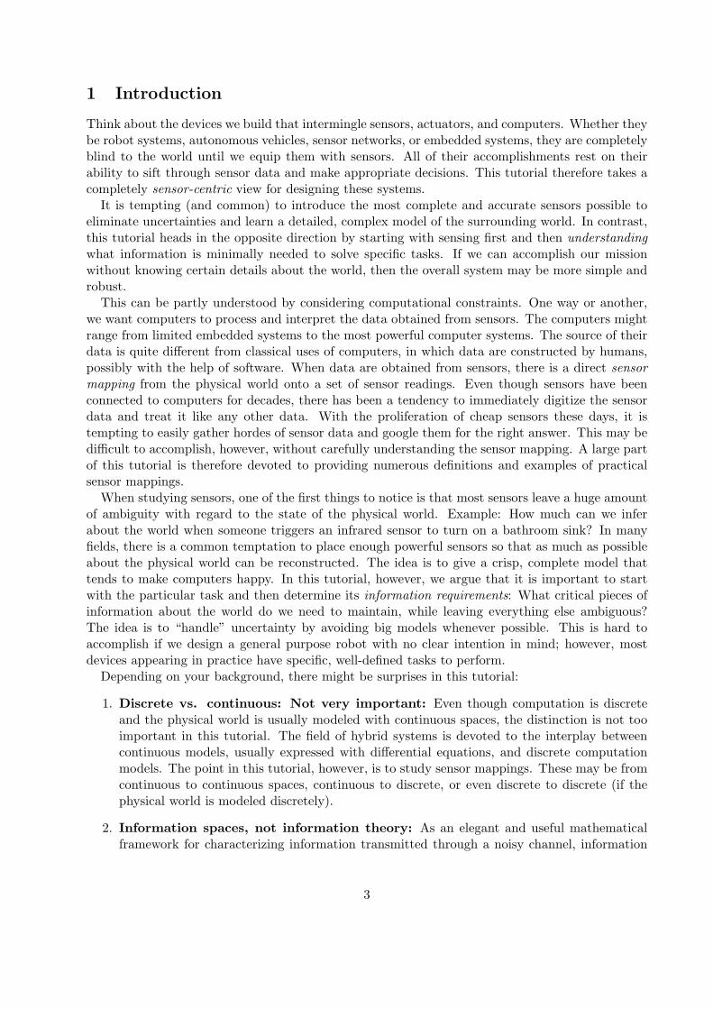


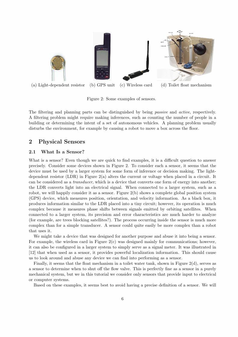


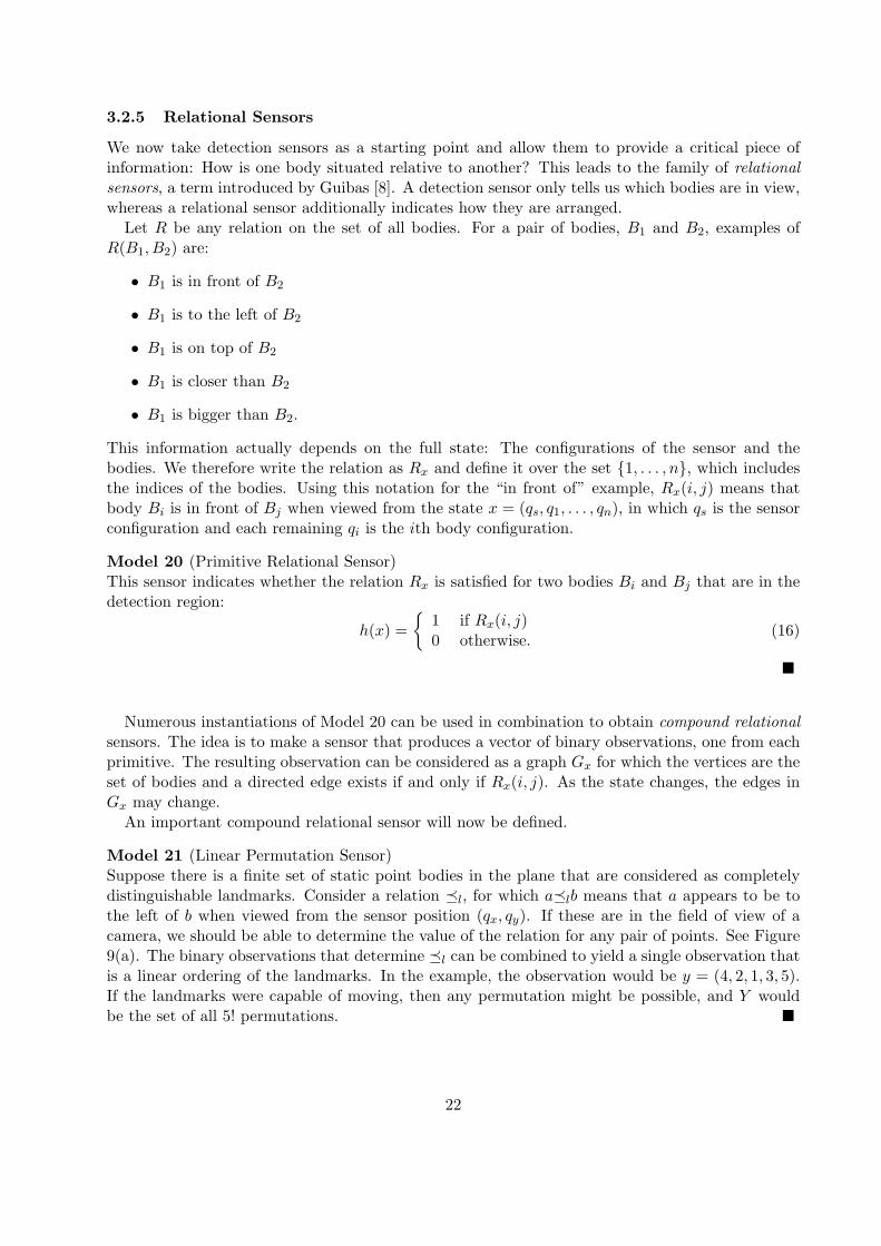


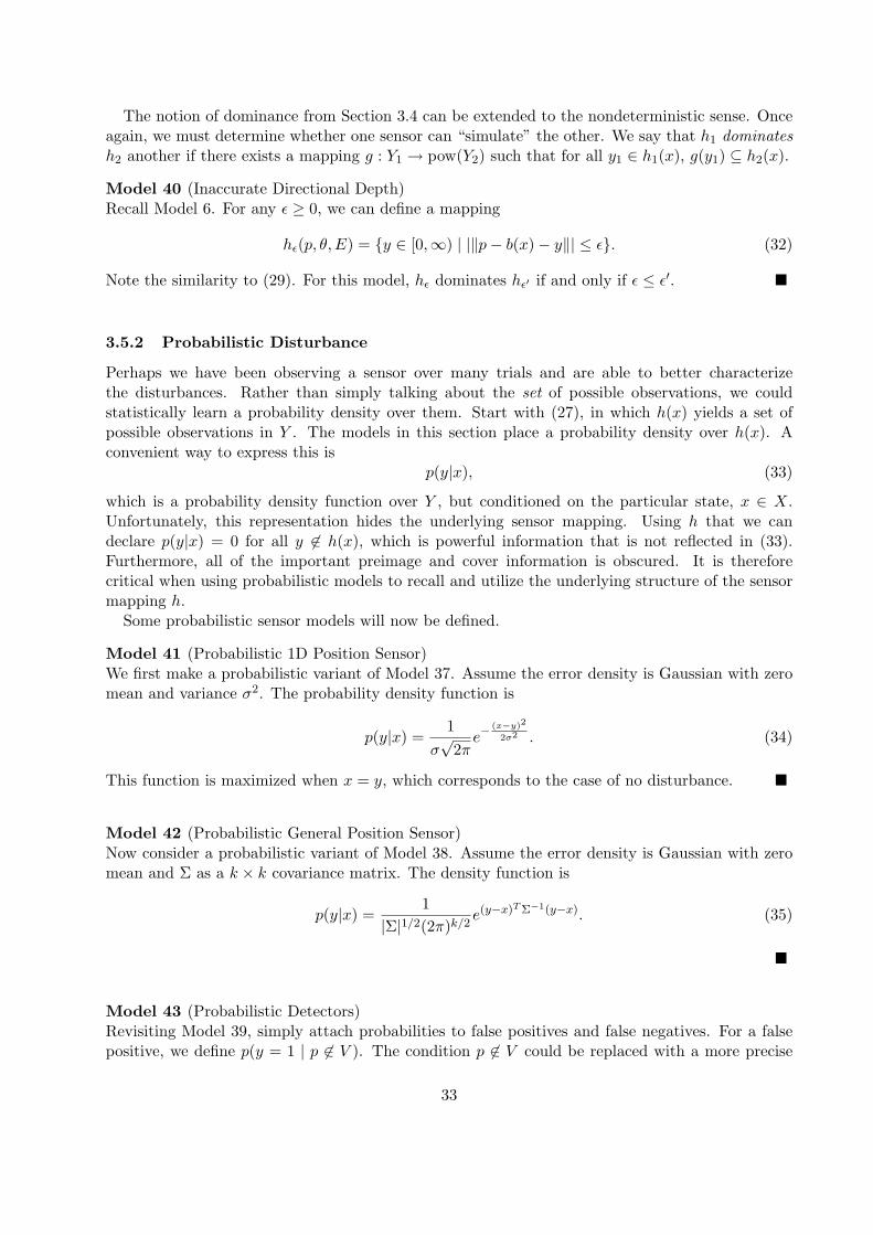


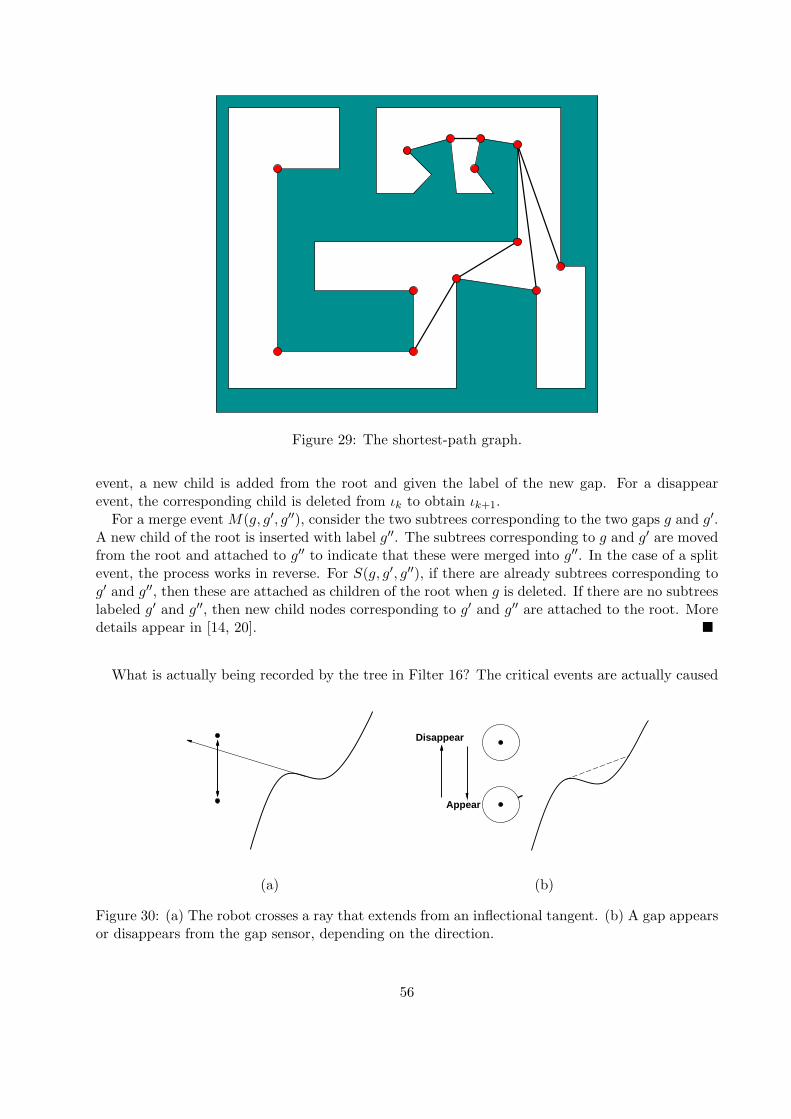


![Robotic Motion Planning: RRT’smotionplanning/lecture/lec20.pdf · 2007. 11. 5. · Rapidly-Exploring Random Trees (RRTs) [Kuffner, Lavalle] The Basic RRT single tree bidirectional](https://static.documents.pub/doc/80x56/60f00c9195ca203cda2c94d8/robotic-motion-planning-rrtas-motionplanninglecturelec20pdf-2007-11-5.jpg)


