FINAL A Front 5.11 - Baylor

FINAL REPORT Freshwater Wetland Functional Assessment Study Contract No. 582-7-77820

Chicken Road study site, Brazoria National Wildlife Refuge

Margaret Forbes, Robert Doyle Adam Clapp, Joe Yelderman,

Nick Enwright and Bruce Hunter

May 2010

Freshwater Wetland Functional Assessment Project TCEQ Contract 582-7-77820

i

FINAL REPORT

Freshwater Wetland Functional Assessment Study

Prepared by

Margaret Forbes and Robert Doyle Baylor University

Center for Reservoir and Aquatic Systems Research

Joe Yelderman and Adam Clapp

Baylor University Geology Department

Nick Enwright and Bruce Hunter

University of North Texas Center for Remote Sensing and Land Use Analyses

Under agreement with

Galveston Bay Estuary Program and

Texas Commission on Environmental Quality Contract # 582-7-77820

PREPARED IN COOPERATION WITH THE TEXAS COMMISSION ON ENVIRONMENTAL QUALITY AND THE U.S.

ENVIRONMENTAL PROTECTION AGENCY - THE PREPARATION OF THIS REPORT WAS FINANCED IN PART THROUGH GRANTS FROM THE U.S. ENVIRONMENTAL PROTECTION AGENCY THROUGH THE TEXAS COMMISSION ON

ENVIRONMENTAL QUALITY.

THIS IS A REPORT OF THE COASTAL COORDINATION COUNCIL PURSUANT TO THE NATIONAL OCEANIC AND

ATMOSPHERIC ADMINISTRATION AWARD NO. NA07NOS4190144.

May 2010


ii

TABLE OF CONTENTS Section Page Table of Contents ............................................................................................................................. ii

List of Tables .................................................................................................................................. iii

List of Figures .................................................................................................................................. v

Executive Summary ...................................................................................................................... viii

A. Introduction ............................................................................................................................... 1

Project Overview ....................................................................................................................... 2

Study Design ............................................................................................................................. 3

Study Area ................................................................................................................................. 3

Study Sites ................................................................................................................................. 8

Literature Cited ........................................................................................................................ 23

B. Functional Assessment Models .............................................................................................. 25

Introduction ............................................................................................................................. 26

Methods ................................................................................................................................... 26

Results ..................................................................................................................................... 29


C. Hydrologic Assessment ........................................................................................................... 43

Introduction ............................................................................................................................. 44

Methods ................................................................................................................................... 45

Results and Discussions .......................................................................................................... 49

Conclusions ............................................................................................................................. 66


D. Water Quality Assessment ...................................................................................................... 70

Introduction ............................................................................................................................. 71

Methods ................................................................................................................................... 71

Results ..................................................................................................................................... 73

Conclusions ............................................................................................................................ 92


E. GIS Application ....................................................................................................................... 96

Introduction ............................................................................................................................. 97

Methods ................................................................................................................................... 97

Results ................................................................................................................................... 107

Error and Uncertainty ............................................................................................................ 118


iii

Conclusions…………………………………………………………………………………126

Literature Cited ...................................................................................................................... 127

APPENDICES ............................................................................................................................. 128

Appendix I – Percent Cover Vegetation ................................................................................ 129

Appendix II – Model Variable Data ...................................................................................... 131

Appendix III – Physical Chemical Soil Characteristics ....................................................... 147

Appendix IV – Water Quality Data…………………………...............................................149

Appendix V – Hydrographs for Random Sites ...................................................................... 180

Appendix VI – LiDAR Elevation Error Analysis ................................................................. 187

LIST OF TABLES Table A1. Climate Normals: Houston Hobby Airport . .............................................................7 Table A2. Summary characteristics of wetland sites ...............................................................10 Table B1. Interactions between model variables and their mathematical expressions. ...........29 Table C1. Turtle Hawk seasonal water budget. .......................................................................52 Table C2. Kite Site seasonal water budget. .............................................................................52 Table C3. Chicken Road seasonal water budget. .....................................................................53 Table C4. Wounded Dove seasonal water budget. ..................................................................53 Table C5. LeConte seasonal water budget. ..............................................................................54 Table C6. Sedge Wren seasonal water budget. ........................................................................54 Table C7. Catchment and wetland areas of the six wetlands. ..................................................56 Table C8. Runoff calculations of three similar magnitude PPT events. ..................................56 Table C9. Average PPT, number of days inundated, discharge volume, and days with discharge for the six monitored wetland. ........................................................63 Table D1. Parameters ..............................................................................................................72 Table D2. PPT dates and sites ..................................................................................................74 Table D3. Depth and YSI data .................................................................................................75


iv

Table D4. Nutrient medians .....................................................................................................76 Table D5. PAH ........................................................................................................................89 Table D6. Phosphorus comparison among sites .....................................................................90 Table D7. N comparison among sites ......................................................................................91 Table E1. Source and description of geodatabases used to estimate variables. .......................98 Table E2. Distribution of hydroperiod type by count and area. .............................................113 Table E3. Functional assessment model variables, field/laboratory methods and GIS databases. ................................................................................................119 Table E4. Comparison of water regime for six study sites and observed inundation ............120 Table E5. Comparison of NDVI derived vegetation cover and field surveys .......................122 Table E6. Comparison of soil pH as measured in lab and from GIS SSURGO database .....................................................................................…123 Table E7. Comparison of soil clay content as measured in lab and from GIS SSURGO database. .......................................................................................124 Table E8. Comparison of land use categories with observed land use ..................................124


v

LIST OF FIGURES Figure A1. Flow chart of project activities ...................................................................................5 Figure A2. Study area consisting of 32 USGS 7.5-minute quadrangles. ......................................6 Figure A3. Location of six initial wetland study sites and six randomly selected sites ...............9 Figure A4. Wounded Dove and Chicken Road with water level monitoring equipment ..........11 Figure A5. Aerial view of Wounded Dove and Chicken Road ..................................................12 Figure A6. Photos of monitoring equipment at Turtle Hawk and Kite Site ...............................13 Figure A7. Aerial view of Kite Site and Turtle Hawk ................................................................14 Figure A8. Photos of monitoring equipment at LeConte and Sedge Wren ................................15 Figure A9. Aerial view of LeConte and Sedge Wren .................................................................16 Figure A10. Photos of installing monitoring equipment at Killdeer and Senna .........................17 Figure A11. Aerial view of Killdeer and Senna .........................................................................18 Figure A12. Photos of monitoring equipment at Dow Chemical and League City ....................19 Figure A13. Aerial view of Dow Chemical and League City .....................................................20 Figure A14. Photos of University of Houston and Harris County ..............................................21 Figure A15. Aerial view of University of Houston and Harris County ......................................22 Figure B1. Ammonia and nitrate removal ..................................................................................33 Figure C1. Wounded Dove hydrograph during Hurricane Ike ..................................................48 Figure C2. Water level at KS weir after Hurricane Ike ..............................................................49 Figure C3. Monthly PPT at Anahuac sites compared to “normal” PPT .....................................50 Figure C4. Monthly PPT at Brazoria sites compared to “normal” PPT ....................................50 Figure C5. Monthly PPT at Armand sites compared to “normal” PPT. ....................................51 Figure C6. Chicken Road 2008 and 2009 hydrograph ..............................................................57


vi

Figure C7. Wounded Dove 2008 and 2009 hydrograph ............................................................58 Figure C8. Turtle Hawk Bird Blind 2009 water level hydrograph .............................................59 Figure C9. Kite Site 2009 weir and interior pond hydrographs ..................................................60 Figure C10. Sedge Wren 2008 and 2009 hydrograp...................................................................61 Figure C11. LeConte 2008 and 2009 hydrograph ......................................................................62 Figure C12. SW discharge event 10/21/2009 – 1/27/2010 .........................................................63 Figure C13. Chicken Road August 2008 water level hydrograph ..............................................64 Figure D1. DO comparison of sites to PPT…… ........................................................................78 Figure D2. TSS comparison of sites to PPT ...............................................................................79 Figure D3. Photo of Wounded Dove ..........................................................................................79 Figure D4. PO4 comparison of sites to PPT ................................................................................80 Figure D5. TP comparison of sites to PPT .................................................................................81 Figure D6. NH4 comparison of sites to PPT ...............................................................................83 Figure D7. NO3 comparison of sites to PPT ...............................................................................84 Figure D8. TN “JMP” comparison of sites to PPT .....................................................................86 Figure E1. Example of flow direction from cell to cell on a DEM ............................................99 . Figure E2. Profile view of a sink as identified on a DEM ........................................................100 Figure E3. Example of a conjoined NWI wetland system ........................................................101 Figure E4. Example of catchment delineation in Harris County using ArcHydro “sink watershed delineation” method ....................................................102 Figure E5. Two small NWI wetlands in Harris County ..........................................................103 Figure E6. Conceptual cross-section of filling a DEM-depression using GIS “fill sinks” function .........................................................................................104 Figure E7. Example of a NAIP image converted to an NDVI image ......................................106


vii

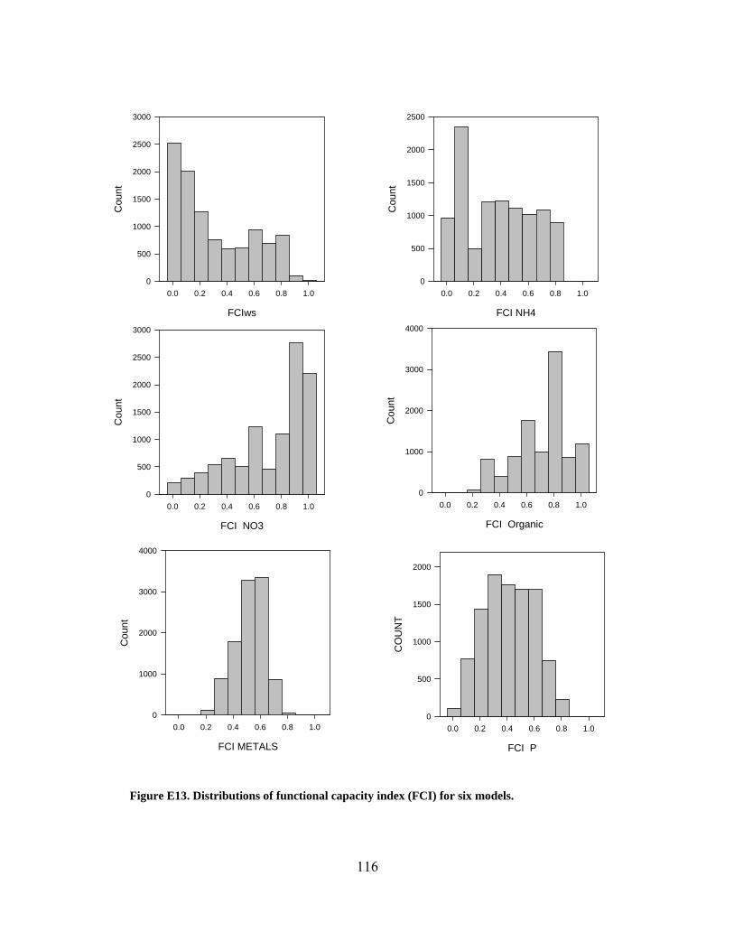
Figure E8. Pie charts of number of wetlands by class and wetland area by class ....................108 Figure E9. Histograms for LiDAR delineated and 100-m buffer strip catchment areas ..........110 Figure E10. Histograms for VcatchRAW (Wetland Area:Catchment Area) ............................111 Figure E11. Histogram of wetland volumes ..............................................................................111 Figure E12. Distribution of model variables Vwet VLU, VsoilpH, Vmac, Vbuff and Vclay ................114 Figure E13. Distributions of functional capacity index (FCI) for six models ...........................116


viii

Executive Summary

Palustrine wetlands are the fastest disappearing wetland type in coastal Texas, and

development pressure is only expected to increase in the area around Houston and Galveston

Bay. The cumulative impact of wetland losses could have substantial detrimental impacts on the

hydrology, water quality, and general ecosystem health of regional aquatic systems, including

Galveston Bay and its tributaries. Although freshwater wetlands are abundant in the 32

quadrangle area around the bay, few quantitative data exist to evaluate the pollutant reduction

and flood storage effectiveness of these coastal prairie wetlands (CPWs). In fact, there is little

hydrologic or water quality data on CPWs in general. Such information is critical for developing

linkages between wetland functions and the environmental integrity of jurisdictional waters such

as Galveston Bay.

To better understand the value of these wetlands, our project assessed their water storage

and water quality functions by conducting field studies and constructing functional assessment

models. The study was designed to: (1) evaluate the capacity of CPWs to store water from

precipitation events; (2) evaluate the water quality function of CPWs; and (3) develop water

quality and flood storage functional assessment models that can be applied through a Geographic

Information System (GIS) to similar wetlands within the study area. The results of this study will

provide a basis for estimating their cumulative value on a regional scale.

CPWs are a component of the globally imperiled Coastal Prairie Ecosystem (USGS

2000). According to our analyses of NWI data, there are 10,349 palustrine wetlands within the

32 quad study area. The total area covered by these wetlands is approximately 512 km2; or 9.5%

of the 5,376 km2 study area. When their catchment areas are included, they cover 28.9% of the

landscape. On an areal basis the largest CPW class is emergent (42,313 ha, 83%) followed by

forested (4,987 ha, 10%), unconsolidated bottom (2,080 ha, 4%) and scrub/shrub (1,735 ha, 3%).

Two thirds of the total wetland area is classified as temporarily or seasonally flooded, and much

of the remaining third are classified as “farmed” and are primarily the large tracts located in

Chambers County. Although the typical CPW is small (<1 ha), we estimate that their total

volume is approximately 47,000,000 m3 (38,535 ac-ft).

We selected six CPW sites for a detailed study of water quality and hydrology, and later

randomly selected additional sites to further evaluate wetland functions. At each sites we

installed water level recorders, and at some sites tipping bucket rain gages and weirs were also


ix

installed. From these data we described each site’s hydroperiod and constructed water budgets

that model runoff, evapotranspiration, and storage volumes. Runoff acounted for an average of

48% of water entering the wetlands, ranging from 5.9% to 89.5%. Runoff estimates were highly

variable both temporally and seasonally and were strongly affected by catchment size and

climate. Potential evapotranspiration losses (as a percentage of total water losses) ranged from

43% to 94% with an average of 69%, supporting assumptions that this is the major pathway for

wetland water losses. Despite drought conditions for much of the study, all six wetlands

overflowed during the monitoring period. The average duration of outflow was 27 days. On a

volume basis, the six wetlands stored an average of 82% of incoming water and discharged 18%.

Patterns of storage and discharge were strongly influenced by antecedent moisture conditions.

These results, combined with the preliminary water level data from six additional CPWs,

indicate that discharge appears to be a regular feature of most CPWs.

Surface water quality sampling was conducted on approximately 9-10 dates at the initial

six CPWs. We also collected and analyzed precipitation as their primary source. Inorganic

nitrogen levels, which can be particularly high in precipitation, has been linked to eutrophication

of coastal waters in the Gulf of Mexico and to algal blooms in Galveston Bay. We found that

each wetland was capable of reducing incoming nitrate-nitrogen by approximately 98%,

regardless of land use, hydroperiods, or other model variables. Ammonia in wetland surface

water was also significantly lower than in precipitation. Phosphate-phosphorus was not

statistically different in wetland surface water than in precipitation. As expected, total nitrogen

and total phosphorus levels were higher in CPWs than in precipitation due to increases in the

organic component of these nutrients. The export of fixed carbon and nitrogen to estuaries and

other receiving waters is acknowledged as a valuable wetland function (i.e. food chain

export/support) and these data confirm that coastal freshwater wetlands lower inorganic nutrient

concentrations and produce organic material both to support local biota and for export to

receiving waters. We found no evidence of nutrient saturation or persistent water quality

degradation at the twelve wetlands.

To model water quality and water storage function, we developed six conceptual models

that predict a CPW’s capacity for (1) water storage, (2) nitrate removal (3) ammonia removal, (4)

phosphorus removal, (5) heavy metal removal, and (6) removal of organic compounds. The

models were derived from literature reviews and are largely theoretical. They do not measure


x

water quality function but rather, provide a relative estimate of the type and degree of functions

that would be gained or lost in wetland conversions. The six models were comprised of variables

that were obtained and applied through GIS and applied to all palustrine wetlands in the 32-

quadrangle study area. They included geomorphic variables (volume, relative catchment size),

hydrologic variables (water regime), soil characteristics (clay content, pH), vegetation (density)

and land use.

Application of the models to the 10,349 CPWs resulting in the following generalizations:

(1) Most of the models resulted in a normal or nearly normal distribution. (2) The water storage

model was skewed toward lower function by approximately 1,000 wetlands that are excavated or

impounded. Removal of these wetlands resulted in a nearly normal distribution of water storage

model values. (3) The phosphorus, ammonium-N and heavy metal models indicated that CPWs

have a moderate capacity for retaining/removing these pollutants.(4) The organic and nitrate

models predicted that many CPWs have a high capacity for removing these pollutants. We were

able to compare the nitrogen and phosphorus models to our field sampling; however we did not

have evidence of organic or heavy metal loading with which to evaluate these models. Most of

the precipitation and wetland samples analyzed for organics and heavy metals were below

analytical detection limits. There was considerable disagreement between soil characteristics as

mapped in soil databases and as evaluated in the field; however LiDAR derived elevations, water

regimes, and land use characterizations were more reliable.

1

A. Introduction

Sabatia campestrus and Limnosciadium pinnatum, LeConte wetland, Chambers County, 27 April 2008

2

Project Overview

Palustrine wetlands in the Houston-Galveston area are being destroyed at an alarming

rate, in part due to the recent Supreme Court rulings that removed many small wetlands from

federal jurisdiction. They are the fastest disappearing wetland type in the area, making up almost

36% of wetland permits issued in Texas between 1991 and 2003 (Brody et. al. 2008). In Texas,

population by shoreline kilometer was projected to double between 1960 and 2010 to 1,216

people per km, which makes the Texas Coast one of the fastest growing coastal regions in the

country (Culliton et al. 1990). Inevitably, the increases in tourism, recreation, commercial

projects, and residences will accelerate wetland alterations and may have negative impacts on

local watersheds. The cumulative impact of wetland losses could also have substantial

detrimental impacts on the hydrology, water quality, and general ecosystem health of nearby

aquatic systems, particularly in Galveston Bay and its tributaries.

Few quantitative data exist to evaluate the pollutant reduction and flood storage

effectiveness of coastal prairie wetlands. In fact, there is little hydrologic or water quality data on

freshwater coastal prairie wetlands (CPWs) in general. Such information is critical for

developing linkages between wetland functions and the environmental integrity of jurisdictional

waters such as Galveston Bay. To better understand the cumulative value of these wetlands, our

project assessed their water storage and water quality functions. The study was designed to: (1)

evaluate the capacity of freshwater wetlands to store water during precipitation events; (2)

evaluate the role of freshwater wetlands in maintaining water quality; and (3) develop water

quality and flood storage functional assessment models that can be applied through a Geographic

Information System (GIS) to similar wetlands within the study area. The results of this study will

provide a more quantitative understanding of how CPWs perform water storage and water

quality functions, and provide a basis for estimating their cumulative value on a regional scale.

This report summarizes project activities for the period August 22, 2007 through

December 31, 2009. It includes an evaluation of the hydrologic and water quality monitoring at

12 field sites that are considered representative of wetlands throughout the study area. The report

also describes the methods, results, and error associated with GIS based water storage and water

quality models that were applied to over 10,000 wetlands in the study area.

3

Study Design

This project consists of four distinct components: 1) development of functional

assessment models for water quality and water storage; 2) GIS application of these models; 3)

hydrologic monitoring of selected CPWs; and 4) water quality monitoring of selected CPWs.

These components and associated deliverables are related as shown in Figure A1. Briefly,

conceptual models for water storage and various water quality functions were developed based

on literature information. Field sampling provided data to evaluate and modify the models and to

increase our understanding of the function and variability of CPWs. Models were finalized and

applied to all CPWs in the study area. These results were then summarized and evaluated with

respect to their distribution. To evaluate the error associated with the models, we compared field

data on the model variables to data predicted using the GIS databases and algorithms. Final

deliverables include electronic maps, databases, reports, and manuscripts.

Study Area

The study area is composed of 32 USGS 7.5-minute quadrangle maps (Fig. A2), which

includes the 30 quads analyzed by White et al. (1993). Wetlands included in this study are all

palustrine, and include ponds, emergent, scrub/shrub, forested and aquatic bed classes as mapped

in the National Wetland Inventory (NWI) database.

Coastal Prairie Wetlands (CPWs) are a component of the globally imperiled Coastal

Prairie Ecosystem (USGS 2000). This southernmost extension of the tall-grass prairie is a mosaic

of depressional wetlands, and flats interspersed with pimple mounds (Moulton and Jacob 2000).

Smeins et al. (1992) described the area as a “clay plain” due to the impervious soils and lack of

incised drainageways. The geology of the study area is Pleistocene, Beaumont Formations

characterized by fluvial-deltaic sediments. The Beaumont Formation includes meanderbelt sand,

floodplain-overbank mud and mud veneer, and circular to irregular depressions on distributary-

fluvial sands which appear to be remnants of abandoned channels (McGowen et al. 1976). The

relict depositional topography consists of meanderbelt ridges with local relief of 1.5 to 3 m and

lower floodbasins. The meanderbelt ridges have loamy and sandy soils, pimple mounds,

undrained depressions, and segments of meandering stream channels (Aronow, S., 1986). The

lower floodbasins have clayey and loamy soils that have high shrink-swell potential.

4

CPWs are characterized by microtopography and complex patterns of inundation that

promote diverse plant communities. Some of these freshwater wetlands originated from ancient

channel scars that have been reworked by aeolian erosion, while other “gilgai” wetlands are

formed by the vertical action of clay soils (Sipocz 2002). The dominant soil types are Vertisols

and Alfisols that developed over Pleistocene deposits flanking the Gulf coast. These wetlands

have diverse and locally variable hydrology, ranging from temporarily flooded to intermittently

exposed. Freshwater CPWs tend to have small watersheds, seasonal inundation, intermittent

outflows, and hydrology driven largely by precipitation and evapotranspiration.

5

Figure A1. Flow chart of project activities.

Although few data have been collected to quantify the basic hydrologic and water quality

processes in freshwater CPWs, recent analysis indicates that cumulative impacts from small

water bodies on regional and global processes such as carbon cycling may be vitally important

Annotated Bibliography

Compile GIS layers (surface

waters-NWI, watershed boundaries, soils, cover)

Evaluate models through

collection of water quality/water storage data

Stakeholder meetings / site visits, develop work plan

Construct conceptual assessment model

Refine models

Apply variables

calculate functional indices with GIS model

Produce maps and GIS matrix showing CPWs

and indices

Final report with model documentation and

methodology for field verification

Publish 2 peer-reviewed articles

6

(Downing et al. 2006). Unfortunately, CPWs are being lost at an alarming rate, particularly those

within Harris County, Texas (Houston area) where 13 % disappeared between 1992 and 2002

(Jacob and Lopez 2005). Their new status as “geographically isolated” from navigable waters

(Comer et al. 2005) puts them at even greater risk.

Figure A2. Study area consisting of 32 USGS 7.5-minute quadrangles.

7

Climate

Climate in the region is described as humid subtropical and is dominated by warm, moist

tropical air masses from the Gulf of Mexico brought landward by the prevailing south-easterly

winds. Annual precipitation (PPT) in the study area is approximately 127 cm (50 inches),

ranging from approximately 110 cm (44 inches) to 137 cm (54 inches) from southwest to

northeast respectively. PPT typically has the highest monthly totals from May to September and

lowest totals from February to April with the rest of the months receiving relatively moderate

PPT (Table A1). An important feature of the upper Gulf coastal climate is the occurrence of

tropical storms and hurricanes that can drop a large amount of PPT in a short period of time

accompanied by high winds. Landfall of these storms is infrequent, but these disturbances

contribute to the long-term hydrology and natural history of the region (Smeins et al. 1992).

Temperatures range from an average low of 7°C (45° F) in January to an average high of 34°C

(94° F) in August; the mean annual temperature is approximately 21°C (70° F). Temperature

ranges become wider farther inland as the buffering ability of the Gulf diminishes. Table A.1

contains monthly and annual mean values for PPT and temperature.

Table A1. Climate Normals: Houston Hobby Airport (source: National Weather Service, 1971-2000).

Month Jan Feb Mar Apr May Jun Jul Aug Sep Oct Nov Dec Year

Mean PPT (cm) 10.8 7.6 8.1 8.8 13.0 17.4 11.1 11.5 14.3 13.4 11.5 9.6 137.1

Mean Temp (° F) 54.3 57.7 64.2 70.0 77.0 82.3 84.5 84.4 80.5 72.2 63.0 56.1 70.5

Average High (° F) 63.3 67.1 73.6 79.4 85.9 91 93.6 93.4 89.3 82 72.5 65.4 79.7

Average Low (° F) 45.2 48.2 54.8 60.6 68.1 73.5 75.3 75.3 71.6 62.3 53.4 46.7 61.3

Geomorphology

The study area occurs on fluviomarine Quaternary deposits gently sloping towards the

coast, mostly deposited during the Pleistocene (> 10,000 years ago). Pleistocene deposits

occurred as a result of alternating periods of glaciation and fluctuating sea-levels in which

sediments were deposited. Holocene (10,000 years to present) deposits are found closer to the

coast and on the flood plains of the many rivers crossing the landscape (Aronow 2000). Geologic

8

processes and hydrology associated with climate changes are complex and have resulted in a

seemingly homogenous flat landscape; however, slight differences in elevation and variation in

substrate composition contribute to a diverse setting.

Soils in the study area are predominantly Vertisols, which are characterized by high clay

content (up to 65%) and high shrink swell potential. Vertisols have low hydraulic conductivity

and consequently may produce more runoff than other soils. On the other hand, the high shrink

swell potential of these soils results in large surficial cracks in dry periods, which can direct

runoff into the soil until soils become moist and swell resulting in closure of cracks. An

important feature of Vertisols is the microtopography of small depressions and ridges they

develop known as gilgai (Aronow 2000). Depressions associated with gilgai collect water from

immediate uplands leading to variations in soil moisture, drying and cracking (Kishné 2009).

Topographical relief between micro-highs and micro-lows is typically 10 to 40 cm (Nordt et al.

2004).

Meander ridges and channel scars are other important features characterizing the

topography of the study area. These features have been reworked by wind and water resulting in

shallow undrained depressions and distinctive soil patterns crossing the landscape. The elevated

areas associated with these meander ridges are typically underlain by sandier, loamier substrates

than the adjacent depressions. Meander ridges and channel scar depressions occur on the

landscape as isolated fragments and as patterns extending several kilometers. Many of the

topographical features discussed above have disappeared due to row-crop tillage, pasture

improvement, drainage ditching, land-leveling and levee construction (Aronow 2000).

Study Sites Six wetland sites were initially selected for hydrologic and water quality monitoring, as

well as to assess general wetland characteristics that relate to the functional assessment models.

The six sites were selected with input from the project Advisory Group. The sites, located in

pairs to facilitate sampling of precipitation, were located at Brazoria National Wildlife Refuge

(NWR), Armand Bayou Nature Center, and Anahuac NWR (Fig. A3, red markers).

During Phase II, six additional sites were selected (Fig. A3, green markers). The advisory

group requested that additional sites be located outside the 100-yr floodplain; therefore, we

randomly selected 70 wetlands outside the floodplain and attempted to obtain permission for

9

access. From the randomly selected wetlands, we added four sites (DW, SE, LG, UH). After

failed efforts to secure the final two sites on Exxon property, we included the fifth site near SE

(KIL). The final site (HA) was added at the request of the Project Manager despite the fact that it

was not within the study area. We did not calculate model indices for that site due to lack of GIS

coverages. Table A2 summarized characteristics of the twelve sites.

Wetland sites were assessed for their soils and vegetation, as well as land use, and other

characteristics related to the model variables. The hydrology of the initial six sites was

characterized for nearly 18 months concurrent with water quality sampling. The random sites

were sampled for water quality at least twice. Over the course of the study, many of the sites

were impacted by hurricanes, drought, hogs, spraying, mowing, or other disturbances. We

describe these events further in the report as they potentially impacted sampling results.

Figure A3. Locations of six initial study sites (red) and six randomly selected sites (green). DW=Dow, CR=Chicken Road, WD=Wounded Dove, LG=League City, UH=University of Houston, KS=Kite Site, TH=Turtle Hawk, HA=Harris, KIL=Kildeer, SE=Senna, SW=Sedge Wren, and LC=LeConte.

10

Table A2. Summary characteristics of wetland sites included in hydrologic and water quality sampling. Hydrologic monitoring began at the initial six sites in May-June 2008 and in July-Dec 2009 at the random sites.

Site

NWI Code

Size (ha)

Longitude (W)

Latitude (N)

Within 100-yr Floodplain?

Land Ownership

CR PEM1C 0.53 95.28740 29.10366 Yes Brazoria National Wildlife Refuge

WD PEM1C 1.54 95.27451 29.11055 Yes Brazoria National Wildlife Refuge

TH PFO1A 4.82 95.07763 29.59315 No Armand Bayou Nature Center

KS PFO1A 3.44 95.06553 29.59794 Partially Armand Bayou Nature Center

SW PEMf 2.39 94.46955 29.67314 Yes Anahuac National Wildlife Refuge

LC PSSf 1.05 94.43611 29.67100 No Anahuac National Wildlife Refuge

DW PEM1C 0.97 95.35685 29.02015 No Dow Chemical

LG PEM1A 9.60 95.01972 29.51859 No City of League City

UH PFO1A 1.58 95.09415 29.58777 No University of Houston

HA PEM1C 1.00 95.13431 29.61630 No Harris County

KIL PEM1F 1.62 94.70628 29.57501 No Private rancher

SE PEM1A 0.20 94.70388 29.57519 No Private rancher


11

Chicken Road and Wounded Dove

Chicken Road (CR) and Wounded Dove (WD) are emergent wetlands consisting mostly as

thick grasses, rushes, and sedges (Fig. A4). Abundant vegetation at CR (Appendix I) was dominated

by Cyperus articulatus, Spartina patens, Ipomoaea sagittata, Paspalum vaginatum and patches of

Juncus roemerianus. Wounded Dove was dominated by Spartina patens, Cyperus articulatus,

Ipomoaea sagittata,and Eleocharis montevidensis. Historically, land in the area was used for livestock

pasture; presently the land is actively managed to maintain prairie habitat. The landscape is extremely

flat (0 – 1% slopes), gently sloping towards the Gulf of Mexico. CR occurs within an ancient channel

scar (Fig. A5) surrounded by upland on either side of the channel with approximately 1 m difference

between the highest upland and the deepest part of the wetland. CR collects runoff from the

surrounding upland. In times of sufficient rain, water may flow into CR from depressions farther up

the ancient channel than those in its immediate catchment area. Once CR’s depression fills up, water

flows out through a culvert as it continues through the channel scar. WD is located approximately 1

mile east of CR on Gilgai formation characterized by microhighs and microlows differing by

approximately 30 cm in altitude. WD does not have a visible channelized outlet. WD is the least

disturbed, most pristine CPW of the 12 study sites.

Figure A4. Wounded Dove (left) and Chicken Road (right) with water level monitoring equipment.


12

Figure A5. Aerial view of Wounded Dove (top) and Chicken Road (bottom) showing study area (aqua) and NWI boundaries (blue), water level recorders (red triangles), piezometers (yellow square), and sampling locations (aqua circles). Note different scales on top and bottom panels.


13

Turtle Hawk and Kite Site

Turtle Hawk and Kite Site wetlands are located at the Armand Bayou Nature Center, which

consists of over 1,000 ha adjacent to Armand Bayou. TH is a forested wetland characterized by many

small depressions. The deepest recorded water depth before overflow was approximately 12 cm.

Discharge occurs through a culvert draining into Armand Bayou. The vegetation is multi-storied with

the overstory dominated by Ulmus americana, Sapium sebiferum (Chinese tallow), and Querca

falcata. The understory consisted of Sabal minor, Vitis rotundifolia, and other vines and saplings;

while the ground cover was dominated by leaf litter, Chasmanthium laxum, Polygonum spp, and

Saccharum giganteum. Kite site is an emergent, scrub/shrub, and forested wetland mapped on

Beaumont Clay, a common soil in the region. Vegetation in the forested area was similar to Turtle

Hawk and the rest of the sites was a mixture of Sabium sebiferum, sedges, and Saccharum giganteum.

A maximum depth at KS of approximately 35 cm produced discharge from a shallow drainage ditch

that is conveyed across Red Bluff Road to Taylor Lake (Fig. A7).

Figure A6. Photos of monitoring equipment at TH bird blind (left) and KS (right).


14

Figure A7. Aerial view of Kite Site (top) and Turtle Hawk (bottom) showing study area (aqua) and NWI boundaries (blue), water level recorders (red triangles), weirs (green boxes), and sampling locations (aqua circles). Note different scales on top and bottom panels.


15

Sedge Wren and LeConte

Sedge Wren (SW) and LeConte (LC) are located on the eastern side of Galveston Bay within

the Anahuac NWR. Both SW and LC occur on similar clay soils. SW is a restored wetland created by

the USFWS in a site previously farmed in rice (Fig. A8). The site has a water control structure that

conveys discharge to Onion Bayou, an irrigation canal. The maximum observed water depth at SW

was approximately 30 cm. SW has a catchment area delineated by Whites Ranch Road (FM 1985) to

the north and a levee/service road on the other three sides. Vegetation at SW includes Eleocharis

montevidensis, E. quandrangulata, Alternanthera philoxeroides, Diodia virginiana, and Panicum

hemitomum.

LC is located approximately 2 miles to the east of SW on FM 1985. It is adjacent to an

irrigation ditch to the south that is used for rice farming. LC is a smaller wetland with a maximum

depth of approximately 15 cm. LC has a greater slope than the other study sites. It has a road ditch

along its southern boundary(see photo) and we installed a weir and water level recorder in the ditch,

about 30 m upslope of a drainage culvert that conveys runoff to the adjacent irrigation ditch (Fig. A9).

LC is grazed by cattle, sometimes heavily, which made plant identification difficult at times. Plant

species include Alternanthera philoxeroides, Echinochloa sp. Panicum repens, Juncus validus,

Eleocharis sp. and Ludwigia sp.

Figure A8. Photos of monitoring equipment at LC (left) and SW (right). Note damage and wrack at LC from Hurricane Ike


16

Figure A9. Aerial views of LeConte (top) and Sedge Wren (bottom) showing study area (aqua) and NWI boundary of adjacent wetlands (blue), water level recorders (red triangles), weirs (green boxes), and sampling locations (aqua circles). Sedge Wren boundaries were determined by walking the wet perimeter Note different scales on top and bottom panels.

.


17

Killdeer and Senna

Killdeer (KIL) and Senna (SE) are located on private ranch land on the eastern side of

Galveston Bay near Smith Point in Chambers County. Killdeer is a pothole-shaped pond (Fig. A10)

and this morphology appears to be common in the surrounding landscape. Both sites were inundated

with Hurricane Ike storm surge but only KIL is still saline (~7 ppt). According to the landowner, prior

to Ike, Killdeer was densely vegetated with an unknown grass and we saw evidence of thick wrack on

our first visit. No vegetation has reestablished at KIL, but adjacent wetlands have Bacopa sp. E.

quadrangulata, and Sesbania drummondii. SE is a smaller depressional wetland located approximately

100 m east of KIL. Maximum SE water depths were only ~7 cm while KIL depths were over 40 cm.

Vegetation at SE consisted of Centella asiatica, S. drummondii, Panicum scoparium, and Juncus

effusus. Both sites are grazed by cattle and have considerable bare ground. Remnant furrows suggest

cropping was a prior activity. Neither site has a channelized outlet.

Figure A10. Photos of installing monitoring equipment at KIL Aug 2009 (top) and SE Nov 2009 (bottom).


18

Figure A11. Aerial view of Killdeer (left) and Senna (right) showing study area (aqua/green) and NWI boundaries (blue), water level recorders (red triangles), and sampling locations (circles).


19

Dow and League City

Dow Chemical (DW) and League City (LG) wetlands are randomly selected wetlands located

several km apart. DW is in Brazoria County northeast of Freeport, in the far southwestern corner of the

study area and LG is in the northern part of Galveston County. DW is within 1-2 km of a chemical

refinery complex in Brazoria County. Historically, the site probably drained into Oyster Creek;

however, a large berm now separates the wetland from the creek. The site is actively grazed by cattle.

In summer 2009, the site was dry with cracked soils and a monoculture of senna. Hydrologic

equipment was installed in August, 2009 and by October 2009; rains had filled the wetland to over 50

cm depth. Submersed and emergent aquatic vegetation now dominate the site (Fig. A12). Plant species

include Paspalum vaginatum, Sagittaria sp. Echinodorus sp. Alternanthera philoxeroides, and

Nymphaea sp.

LG is a mitigation wetland that is managed by the City of League City. It is actively managed

for Chinese tallow by mowing and since being dry in August has accumulated up to 28 cm of water. A

residential development was recently built on its western boundary. The site contains intact mima

mounds and a strikingly diverse vegetation community including grasses, sedges, and submersed

aquatics. Water appears to discharge through a broad channel off site toward Galveston Bay (Fig.

A13). Plant species include Cyperus virens, Panicum sp. Pluchea foetida, Sapium sebiferum,

Paspalum floridanum, Letpochloa fascicularis, and Proserpinaca palustris and many other grasses

and forbs.

Figure A12. Photos of monitoring equipment at DW (left) and LG (right).


20

Figure A13. Aerial view of Dow (top) and League City (bottom) showing study area (aqua) and NWI boundaries (blue), water level recorders (red triangles), and sampling locations (circles). Note different scales on top and

bottom panels.


21

University of Houston and Harris County

University of Houston (UH) and Harris County mitigation site (HA) are located in developed

areas of Harris County. UH is a forested wetland (Fig. A15) that lies within the Clear Lake UH

campus grounds. The site is bounded on the north by Middlebrook Drive and we have witnessed the

wetland discharge flowing across the sidewalk of this road on two occasions. The southern upland area

adjacent to the wetland is used to dispose of landscaping material. The maximum recorded water depth

at this site was 6-7 cm. Plants species at UH include Rubus trivialis, Lonicera japonica, Sapium

sebiferum, Ulmus americana, Ilex vomitoria and Carex sp.

HA is east of Ellington Field and bisected by Space Center Blvd. HA is similar to LG in its

vegetation and topography (wet prairie). The monitoring equipment was not installed at this site until

December 2009. Plant species were surveyed in April 2010 and included Panicum sp. The site is

managed by Harris County.

Figure A14. Photos of UH (left) and HA (right). The road behind HA is Space Center Blvd.


22

Figure A15. Aerial view of University of Houston (top) and Harris County (bottom) showing study area (aqua) and NWI boundaries (blue), water level recorders (red triangles), and sampling locations (aqua circles). Note different

scales on top and bottom panels. The Harris County NWI boundary is approximate.


23

Literature Cited

Aronow, S. 2000. Geomorphology and surface geology of Harris County and adjacent parts of Brazoria, Fort Bend, Liberty, Montgomery, and Waller Counties, Texas. Unpublished manuscript. Department of Geology, Lamar University, Beaumont, Texas.

Brody, S. D., S. E. Davis, W. E. Highfield, and S. P. Bernhardt. 2008. A spatial-temporal analysis of

section 404 wetland permitting in Texas and Florida: thirteen years of impact along the coast. Wetlands 28:107-116.

Comer, P., K. Goodin, A. Tomaino, G. Hammerson, G. Kittel, S. Menard, C. Nordman, M. Pyne, M.

Reid, L. Sneddon, and K. Snow. 2005. Biodiversity Values of Geographically Isolated Wetlands in the United States. NatureServe, Arlington, VA.

Culliton, T. J., M. A. Warren, T. R. Goodspeed, D. G. Remer, C. M. Blackwell, and J. J. McDonough.

1990. Fifty Years of Population Change along the Nation's Coasts. Rockville, Maryland: National Oceanic and Atmospheric Administration. 41. p.

Downing, J. A., Y. T. Prairie, J. J. Cole, C. M. Duarte, L. J. Tranvik, R. G. Striegl, W. H. McDowell,

P. Kortelainen, N. F. Caraco, J. M. Melack and J. J. Middelburg. 2006. The global abundance and size distribution of lakes, ponds, and impoundments. Limnology and Oceanography 51: 2388–2397.

Jacob, J. S. and R. Lopez. 2005. Freshwater, non-tidal wetland loss, lower Galveston Bay watershed

1992-2002: A rapid assessment method using GIS and aerial photography. Texas Coastal Watershed Program, GBEP 582-3-53336.

Kishné, A. S., C. L. S. Morgan, and W. L. Miller. 2009. Vertisol crack extent associated with gilgai

and soil moisture in the Texas Gulf Coast Prairie. Soil Science Society of America Journal 73:1221-1230.

Moulton, D. W. and J. S. Jacob. 2000. Texas coastal wetlands guidebook. Texas SeaGrant Publication

TAMU-SG-00-605. www.texaswetlands.org 66 pp. Nordt, L.C., L.P. Wilding, W.C. Lynn, and C.C. Crawford. 2004. Vertisol genesis in a humid climate

of coastal plain of Texas, U.S.A. Geoderma 122:83-102. Sipocz, A. 2002. Southeast Texas isolated wetlands and their role in maintaining estuarine water

quality. Paper presented at “The Coastal Society 2002 Conference: Converging Currents: Science, Culture, and Policy at the Coast”, Galveston, Texas.

Smeins, F. E., D. D. Diamon, and C. W. Hanselka. 1992. “Coastal Prairie”, Chapter 13, In, Kusler and

Brooks, eds. Ecosystems of the World 8A Natural Grasslands, pp 269-290. USGS. 2000. Coastal prairie. FS-019-00. National Wetlands Research Center, Lafayette, LA.


24

White, W.A., T.A. Tremblay, E.G. Wermund, Jr. and L.R. Handley. 1993. Trends and status of wetland and aquatic habitats in the Galveston Bay system, Texas. Galveston Bay National Estuary Program GBNEP-31, 144 pp.

25

B. Functional Assessment Models

Robert Doyle at League City wetland, November 2009

26

Introduction

There is abundant evidence that wetlands have the capacity to improve water quality and

provide storage and desynchronization of floodwaters. The inherent capacity to perform these

functions is dependent on the physical, biological, and chemical characteristics of the wetland.

Coastal Prairie Wetlands (CPWs) are an integral part of the Galveston Bay ecosystem, yet their

water quality and flood storage functions have not been evaluated. This report presents six

conceptual models that predict a CPW’s capacity for (1) water storage, (2) nitrate removal (3)

ammonia removal, (4) phosphorus removal, (5) heavy metal removal, and (6) removal of organic

compounds. The models are derived from literature reviews of site specific research studies and

functional assessment models (primarily hydrogeomorphic models) developed for other classes

of wetlands. This literature was used in conjunction with the project team’s professional

judgment and what is known about hydrology and biogeochemical processes in CPWs.

Methods

The models presented in this document are consistent with previous HGM models

derived for depressional wetlands (Gilbert et al. 2006, Lin 2006, Stutheit et al. 2004) and

wetlands in south Florida (Zahina et al. 2001). Our approach to model development also

incorporates some of the general guidelines for HGM modeling presented by Smith et al. (1995).

Most functional assessment approaches predict a wetland’s potential for performing a given

function based on the wetlands’ characteristics such as position in the landscape, morphology,

hydrology, soils, vegetation, etc. The resulting predictive models do not measure whether the

function is actually being performed and such verifications are rarely attempted. Instead,

functional models provide a relative estimate of functional capacity. They typically provide

qualitative values (low, medium or high) or indexed values (0.0 – 1.0) relative to a “fully

functional” reference wetland. Some models (e.g. WET 2.0) include variables that account for

the opportunity the wetland has to perform the function and the social significance of the

function. Other approaches (e.g. HGM) do not include opportunity or social significance

variables. The CPW functional models presented in this report do not include opportunity or

social significance variables. They are also indexed to provide a relative estimate of function

known as the Functional Capacity Index (FCI). The FCI can range from 0.0 – 1.0, where 0.0

27

indicates that the functional capacity is absent and a 1.0 indicating that the wetland functions at a

level similar to the selected reference wetlands. It is important to understand that, although FCI

provides a numerical value for wetland function, that value is relative and may best be

interpreted as low, moderate, or high.

One important difference between the CPW models presented here and existing

hydrogeomorphic (HGM) models is the use of reference wetlands. Development of an HGM

approach for a regional class of wetlands requires extensive data collection in reference

wetlands, which are wetlands believed to be performing at a high functional capacity (Smith et

al. 1995). Data collected in reference wetlands are used to define the range of functionality and

the range of values for predictor variables. Instead of using this somewhat subjective approach,

we will evaluate the wetlands based on how well they perform the function. For example,

wetland # 1 is considered to have a higher ammonium removal function if concentrations of

ammonium are lower in wetland # 1 (relative to rainfall) than in the other wetlands evaluated.

Conversely, if a wetland tends to have higher ammonium levels, it would be considered to have a

lower functional capacity.

Variables used in HGM models characterize relative catchment size, land use, hydrology,

soils, and vegetation. They are assigned values that range from 0.0 to 1.0 scaled to the range of

expected values for the type of wetland. Variables selected for CPW models were defined so as

to allow them to be quantified in the field either by direct measurement or by field indicators.

Because GIS methods will be utilized to apply the models to CPWs in the study area, it was also

necessary that each variable be applicable using GIS databases.

The final step in conceptualizing the assessment model is to develop an aggregation

equation that combines model variables and derives the FCI. We used the approach developed by

Smith and Wakeley (2001) for HGM development. In this approach, the types of interactions

between model variables (Table B1) may be additive, where either variable alone or both in

combination contribute to functional capacity. If the sum exceeds 1.0, the FCI is taken to be 1.0.

A limiting relationship is one in which a low value for any one variable lowers the function. This

type of relationship is defined by the minimum of the two variables. It is commonly used in

habitat indices, where factors such as food, cover, or nesting sites are all necessary for survival.

A compensatory relationship occurs when a high value for one variable compensates for a lower

value of another variable. This type of relationship is defined by the maximum value of the two

28

variables. A partially compensatory relationship occurs when two or more variables contribute

equally and independently to the level of function. It is calculated as either the arithmetic mean

or the geometric mean, with the former being more sensitive to low values. Another important

difference between the arithmetic mean and the geometric mean is that with the geometric mean,

if any variable is equal to zero, the resulting FCI is zero. A controlling feature is one that is

critical to the performance of a function. For example, organic carbon export might be modeled

by the following equation: FCI = VFREQ x (VLITTER + VCSD)/2. Carbon export is affected by the

abundance of leaf litter (VLITTER) and coarse woody debris (VCSD), which are grouped and

averaged because they contribute equally and independently to the availability of material for

export. However the export cannot occur until floodwaters scour the site (VFREQ). Thus the

product relationship allows VFREQ to drive the FCI to zero at sites where no flooding occurs,

despite high values of the other variables. Finally, variables may also be weighted if their

contribution to the function is believed to be more important than other variables. Methods and

supporting information for assigning values to model variables are provided in Appendix 1.

The models presented here may be revised to reflect the results of water quality data,

water storage data, and model variable data collected at six CPWs in the study area. For

example, two model variables have been eliminated due to limitations of available GIS

databases. The first variable described the presence of modified wetland outlets. While this

variable may impact water storage function, we could not develop a reliable method for

identifying the presence of such outlets using available GIS databases. The second variable

eliminated was soil organic matter. While potentially important for removal of nitrogen, metals,

and organic contaminants, our laboratory analyses of soil organic matter (loss on ignition

method) did not correlate well with soil organic matter values provided in the Soil Survey

Geographic (SSURGO) database.

29

Table B1. Types of interactions between model variables and their mathematical expression for developing HGM assessment models (adapted from Smith and Wakeley 2001).

Type of Interaction Mathematical Operation Example

Cumulative Addition FCI = VA + VB + VC; if sum > 1.0 then FCI = 1.0

Limiting Minimum FCI = MIN (VA, VB )

Fully compensatory Maximum FCI = MAX (VA, VB )

Partially compensatory Arithmetic mean FCI = (VA + VB + VC )/3

Geometric mean FCI = (VA x VB x VC )1/3

Controlling Product FCI = VA x (VB + VC)/2

Weighted Coefficient FCI = 2(VA + VB + VC)/4

Results

Surface Water Storage Model

Surface water storage is defined as the capacity of a wetland to temporarily store and

convey surface water during rainfall or flood events. This function is often referred to as flood

attenuation or flood peak desynchronization. The primary source of surface water is from direct

precipitation, with a secondary source from overland runoff. The water budget of depressional

wetlands is influenced by precipitation within the catchment, groundwater recharge and

discharge, evapotranspiration, and the configuration of the wetland outlet. In wetlands with flow-

through, density and rigidity of emergent vegetation can retard water velocities by providing

hydraulic roughness. In addition, vegetation may influence evapotranspiration rates. At any

given moment, the water level in the wetland is a balance of these factors.

In general, the underlying geology and soils of the coastal plain area promote slow rates

of exchange between ground water and surface water. In CPWs, therefore, precipitation and

evapotranspiration (EVPT) are believed to play the largest role in determining fluctuations in the

wetland water level (Smeins et al. 1992). Evapotranspiration may be the most important pathway

for water losses in depressional wetlands; annual lake evaporation in the Galveston Bay Area is

approximately 53 inches and annual class A pan evaporation is 70 to 75 inches (Dunne and

Leopold 1978). Rates of EVPT have been shown to be higher in systems with abundant emergent

vegetation. For example, wetlands dominated by broadleaf cattail (Typha latifolia) were

demonstrated to have double or triple EVPT rates of an unvegetated area (Towler et al. 2004).

30

Wetlands with larger surface areas would also have greater potential for total EVPT. A

wetland with higher evapotranspiration rates would be expected to have greater storage function

because a wetland’s capacity for flood attenuation is dependent upon the storage volume

available at the onset of precipitation events. Thus overall wetland size and volume are important

characteristics for predicting flood storage. The ratio of the wetland surface area to the surface

area of its catchment (Vcatch) has been proposed as an important characteristic for evaluating

water storage function (Bradshaw 1991, Fennessy et al. 2004, Lin 2006). Wetlands that can store

at least 25% of the catchment runoff from a 24-hr two-year rain event have been assigned a high

water storage function (Simon et al. 1987, Bradshaw 1991). Water storage and flood attenuation

tend to be greater in wetlands with substantial water level fluctuations, such as those with large

wet meadow zones (Gilbert et al. 2006), or with intermittent, seasonal, temporary, or semi-

permanent hydrologic regimes. Hydrological modifications or modifications that maintain water

in the wetland typically reduce their effective storage volumes.

The conceptual model for water storage (Eq. 1) contains variables for wetland volume

(Vvol), the presence of year-round or nearly year-round water in the wetland (Vwet), the ratio of

wetland size to catchment size (Vcatch) and percent of wetland area that is vegetated with

macrophytes (Vmac). The wetland volume variable can be zero if the wetland has been filled or

modified to drain completely.

(Eq. 1)

Water Quality Models

Wetlands have the ability to remove, reduce, degrade, or provide long-term storage of a

variety of pollutants. Pollutants include elements such as heavy metals, nutrients such as

nitrogen and phosphorus, compounds such as PAHs, herbicides and pesticides, and particulates.

These compounds may enter wetlands through aerial deposition, surface runoff, groundwater

exchange, or through streams or manmade conveyances. A quantitative measure of water quality

function would require a determination of the amount of pollutant removed or retained per unit

area during a specified period of time (e.g. g/m2/year). Such data-intensive studies are rarely

undertaken in the context of functional assessment. Rather, functional assessment models are

⎟⎠⎞

⎜⎝⎛ +

×=2

maccatchwetvolWS

VVVVFCI

31

used by regulators and land use managers to inform decisions regarding proposed activities in

wetlands. In this context, functional assessment models have been used to estimate the type and

degree of functions that would be gained or lost in wetland conversions.

Most HGM models developed for depressional wetlands have used a single model for

retention or removal of nutrients, organics, heavy metals and other contaminants. However, most

contaminants have unique fate and transport pathways. For example, the wetland characteristics

that promote nitrogen removal will not necessarily optimize the removal of other pollutants. To

incorporate our understanding of the fate and transport of specific contaminants in wetlands, we

have developed separate water quality models for nitrogen, phosphorus, selected heavy metals,

and organics.

Nitrogen Retention/Removal

Nitrogen pollution is an important consideration in the Galveston Bay area and near-

shore ecosystems, particularly as anthropogenic inputs associated with development continue to

increase. Nitrogen retention/removal function is defined as the capacity of a wetland to reduce

the water column concentrations of ammonium and nitrate. This may occur through short term or

long term storage of nitrogen in biota and sediments; or through permanent removal of nitrogen

primarily through the nitrification-denitrification process.

Nitrogen may enter CPWs through precipitation, surface runoff, and from direct faunal

deposition. Nitrogen transformations in wetlands may be substantial depending upon the nature

of nitrogen loading as well as characteristics of the individual wetland. Nitrogen is removed from

the water column primarily by four processes (Reddy and Patrick 1984): (1) uptake by plants, (2)

immobilization by microorganisms during plant decomposition, (3) adsorption of ammonium

onto organic matter and clay, and (4) most importantly, through the nitrification-denitrification

process.

The nitrification–denitrification process leads to permanent removal of nitrogen from

wetland systems. Nitrification is the microbially mediated oxidation of ammonium to nitrite and

then nitrate. The process consumes approximately 4.3 grams of oxygen for each gram of nitrogen

oxidized, and therefore occurs primarily in aerobic areas of the wetland (surface waters,

unsaturated soils, rhizospheres of emergent plants, etc.). Once ammonium is oxidized, the

resulting nitrate then diffuses to anaerobic areas of the wetland where it may be denitrified. This

32

transport of the resulting nitrate from aerobic to anaerobic zones has been shown to be the rate

limiting step in the removal of nitrogen from flooded systems (Patrick and Reddy 1976). In

general however, nitrification rates can be limited in wetland systems due to nitrifying bacteria’s

sensitivity to reduced oxygen levels, temperature, toxicity, pH, and competition from bacteria

that oxidize carbon rather than ammonium.

Denitrification is the reduction of nitrate into gaseous nitrous oxide (N2O) and molecular

nitrogen (N2), which are then released to the atmosphere (Mitsch and Gosselink 1993).

Denitrification occurs primarily in reduced soils and sediments where abundant organic matter is

used as a carbon source for denitrifying bacteria. Denitrification has been shown to remove

relatively large quantities of nitrogen from wetlands, particularly when the proportion of nitrate

in incoming loads is high (Nelson et al. 2004).

Because nitrification and denitrification are promoted by different environmental

conditions, their removal depends both on the incoming water and the characteristics of the

individual wetland. For example, wetlands receiving inputs primarily from precipitation or

runoff from undisturbed catchments will likely be able to process incoming nitrogen through the

processes described earlier. In contrast, wetlands receiving runoff from fertilized agricultural

fields or other enriched sources may not be able to nitrify ammonia rapidly enough to achieve

background levels. In this case, a fluctuating hydrologic regime would facilitate nitrification by

enhancing aeration (Figure B1). It has been demonstrated that nitrification is greater in wetlands

where soil moisture contents fluctuate repeatedly (Patrick and Mahapatra 1968, Ponnamperuma

1972, Reddy and Patrick 1975), such as in the wet meadow zone.

In contrast, denitrification rates can be rapid in wetlands during periods of inundation or

soil saturation. Denitrification rates have been shown to increase with higher initial

concentrations of nitrate. Thus higher rates of nitrate removal may occur in wetlands receiving

high nitrate runoff.

33

Figure B1. Conditions that promote ammonia and nitrate removal, and the corresponding functional capacity equations.

Two conceptual models are proposed for predicting nitrogen removal in CPWs. Equation

2 is for ammonium removal and Eq. 3 is for nitrate removal. Both models contain variables for

percent of buffer that is vegetated (Vbuff), and percent of wetland area that is vegetated with

macrophytes (Vmac).

(Eq. 2)

The ammonia model contains two additional variables. The first variable (Vdry) describes

the wetland hydroperiod, which is scaled to reflect the duration of inundation (Table 3, Appendix

I). This variable describes the tendency of the wetland to dry out or draw down, which

theoretically promotes nitrification. Vdry values are high for systems with frequently fluctuating

water levels, such as those classified as seasonally flooded or saturated. Lower values would be

assigned to wetlands classified as permanently flooded or intermittently flooded. The ammonia

model also includes a term for wetland and catchment land use (VLU). This variable is the

AMMONIUM

Removal favored by AEROBIC CONDITION

(frequent drying)

Removal favored by ANAEROBIC CONDITION

(persistent inundation)

EQUATION 3 EQUATION 2

NITRATE

⎟⎠⎞

⎜⎝⎛ ++

×=3

3LUmacbuff

dryNHVVVVFCI

34

observation that surface waters collected from a grazed site appear to have higher ammonia

concentrations than waters collected from non-grazed sites. We used Table 5 (Appendix I),

which was developed from phosphorus concentrations associated with runoff from different land

uses, to assign values to VLU.

(Eq. 3)

Phosphorus Retention Model

Phosphorus retention is defined as the capacity of a wetland to remove phosphorus from

overlying water and provide long-term storage of that phosphorus in sediments, soils, plant

material, or other biota. Although phosphorus removal may occur when vegetation is harvested

or sediment is removed, these processes are difficult to predict and therefore are not considered

in this model.

Phosphorus enters CPWs primarily via wet and dry deposition, surface runoff, and piped

or channelized inflows. Because phosphate has a strong affinity for clay and other mineral

particles, much of an annual phosphorus load may enter wetlands sorbed to particulate matter

during one or two large flood events (McKee et al. 2000). These particulate phosphorus loads

often settle out in wetlands and become a permanent part of the bottom sediments. Thus wetlands

with low water velocities and high hydraulic roughness would be expected to have good

suspended sediment and particulate phosphorus removal. Macrophytes also contribute to total

phosphorus retention by providing hydraulic roughness which slows water velocities and thus

enhances sedimentation of particulate-phosphorus.

The primary mechanisms of wetland phosphorus storage are: (1) microbial uptake by

plankton and periphytic organisms, (2) plant uptake, (3) incorporation of organic phosphorus into

soil peat, and (4) soil adsorption (Richardson 1985). Inside the wetland, phosphorus may be

taken up by plankton and periphyton, but this storage pool is small with rapid turnover.

Macrophytic production may account for measurable phosphorus uptake, however approximately

30-75% of the nutrient is seasonally released back to the water column during senescence, with

⎟⎠⎞

⎜⎝⎛ +

=2

3macbuff

NOVVFCI

35

some permanent storage as peat and litter (Richardson and Craft 1993). Adsorption of dissolved

phosphorus to soil and sediments is the largest retention processes in wetlands with mineral soils.

Whereas the atmosphere is the ultimate sink for nitrogen, the sediment-litter compartment

contains greater than 95% of the phosphorus in natural wetlands (Faulkner and Richardson

1989). Phosphorus associates with sediments through sorption, precipitation, and incorporation

into the crystalline lattice of iron, aluminum and calcium compounds (Nichols 1983). Several

researchers have found that phosphorus sorption to natural and artificial substrates is correlated

to their iron and aluminum contents (Sakadevan and Bavor 1998, Reddy and D’Angelo 1997,

Pierzynski 1991). Although anaerobic conditions can lead to the release of iron-bound

phosphates from sediments, soils with high mineral or clay contents are generally predicted to

have high phosphorus retention capacities (Zahina et al. 2001, Masscheleyn et al. 1992, Cedfeldt

et al. 2000). However, even wetlands with high phosphate-sorbing mineral soils can become

saturated with respect to phosphorus. At high phosphorus loading rates (e.g. wastewater effluent

at concentrations of 2 mg L-1 or higher), wetlands may eventually become a phosphorus source

rather than a sink (Tilton and Kadlec 1979, Forbes et al. 2004).

Wetlands with shallow, slow moving water and dense vegetation would be predicted to

have a high capacity for settling particulate phosphorus. In addition, wetlands with clay soils

would be expected to retain phosphorus at low phosphorus loading rates. Wetlands with high

vegetation production rates and prolonged inundation would also provide some long-term

phosphorus storage through the accumulation of litter and peat (Mitsch and Gosselink 1993). A

conceptual model for phosphorus retention in CPWs (Eq. 4) includes variables for adjacent

buffer (Vbuff), the density of macrophytes (Vmac), and the soil clay content (Vclay). To account for

a wetland’s potential for phosphorus saturation, land use (VLU) and the ratio of the wetland

surface area to catchment surface area (Vcatch) are also included. Note that unimpacted land use

categories such as forested or natural areas will have the highest value (i.e. 1.0) whereas land

uses associated with phosphorus pollution (i.e. agriculture) will have small values (i.e. 0.05).

⎟⎠⎞

⎜⎝⎛ ++

×⎟⎠⎞

⎜⎝⎛ +

=32

claymacbuffcatchLUP

VVVVVIFC (Eq. 4)

36

Heavy Metal Retention Model

Heavy metal retention is defined as the capacity of a wetland to remove heavy metals

from the overlying water and provide long-term storage in sediments, soils or plant material.

Heavy metals enter wetlands from a variety of sources including fertilizer impurities, tire dust,

cement production, wastewater, urban runoff, combustion products of fossil fuels, industrial

sources, and natural sources. The dispersion of heavy metals into the atmosphere, both as

particles and as vapors, often exceeds levels associated with natural releases (Stumm and

Morgan 1996).

There are three primary mechanisms for heavy metal sequestration in wetlands (Kadlec

and Knight 1996): (1) binding to particulates and soluble organics through cation exchange and

chelation, (2) precipitation as insoluble salts, principally sulfides and oxyhydroxides, and (3)

uptake by biota. Studies of heavy metal retention by treatment and natural wetlands indicate that

sediments are the primary storage components for metals, with minor (~2%) retention in plant

tissue (Lesage et al. 2007, Zuidervaart et al. 1999).

There is considerable variation in behavior and removal efficiencies among individual

metals. For example, iron and manganese have been shown to increase in some treatment

wetlands due to their solubilities under reducing conditions (Lesage et al. 2007, Nelson et al.

2004). Mercury is unique for several reasons: it is primarily transported atmospherically, it may

volatilize from sediments to the atmosphere, it may be methylated under anaerobic conditions to

a more toxic form (mono- and dimethyl mercury) which also bioconcentrates in animal tissue.

Due to the unique properties of mercury, this metal is not included in the functional model.

In general, well buffered, alkaline soils and the presence of organic matter or clay

increase the ability of wetlands to remove heavy metals from the water column via sorption and

precipitation. In nonacidic soils with plentiful sulfates, carbonates, or phosphates, metals can

form insoluble complexes (e.g. metal sulfides) and be retained more or less permanently in the

sediments. Soil organic matter may also form stable complexes with metal ions, however this

variable was eliminated due to our inability to represent it with GIS databases. The presence of

vegetation and appropriate soil types adjacent to the wetland (buffer) also enhances retention of

heavy metals by slowing runoff, settling particulates, and facilitating contact with soils. The

functional assessment model for heavy metal retention is shown below (Eq. 5). The index

increases when wetlands contain nonacidic soils, soils with high clay contents, dense macrophyte

37

cover, and vegetated buffers. A low rating is assigned to wetlands with acidic soils or soils that

are low in organic matter or clay, and with sparse vegetation.

32

soilpHclaymacbuff

eMVVVV

IFC++

+

= (Eq. 5)

Organic Compounds Removal

Organic contaminant removal or retention is defined as the capacity of a wetland to

remove or transform organic contaminants present in the water column. Organic contaminants

include a wide variety of compounds, both natural and synthesized. Organics that are of

particular concern for water quality include pesticides, petroleum hydrocarbons, and other

industrial organics such as solvents. Additional pathways for the removal or retention of organics

in wetlands are a function of their tendency to serve as food for microbes and to degrade over

time particularly when exposed to the atmosphere and sunlight. The major pathways for removal

of hydrocarbons from wetlands waters are: (1) volatilization, (2) photochemical oxidation, (3)

sedimentation, (4) sorption, and (5) biological degradation (Kadlec and Knight 1996).

Photochemical oxidation rates are chemical specific. In general, however, longer

hydraulic retention times and shallow water depths should result in greater degradation of

organics via this process. The capacity of an organic contaminant to settle out of the wetland

would be dependent upon its ability to associate with particulate matter. Charged (polar) organics

may associate ionically with clays while nonpolar molecules tend to associate with organic

matter in the wetland. Partitioning of organics between aqueous and solids (particulates,

sediments, etc.) can be predicted to some extent using physicochemical properties of organic

compounds such as the relative partitioning between the liquid octanol and water coefficient

(Kow) and water solubilities (Sawyer et al. 1994).

A conceptual model for removal or retention of organics (Eq. 6) includes variables for a

wetland surface area to catchment surface ratio (Vcatch), density of vegetation (Vmac). Vcatch,

which is correlated to relative hydraulic retention time, is predicted to have a greater role in

functional capacity than vegetation density or soil organic matter.

38

2catchmac

rgoVVIFC +

= (Eq. 6)

39

Literature Cited Adamus, C. L. and M. J. Bergman. 1995. Estimating nonpoint source pollution loads with a GIS

screening model. Water Resources Bulletin 31 :647-655. Antonic, O., D. Hatic and R. Pernar. 2001. DEM-based depth in sink as an environmental

estimator. Ecological Modeling 138:247-254. Baker, J. E., S. J. Eisenreich, and B. J. Eadie. 1991. Sediment trap fluxes and benthic recycling

of organic carbon, polycyclic aromatic hydrocarbons, and polychlorobiphenyl congeners in Lake Superior. Environmental Science and Technology 25: 500-509.

Bradshaw, J. G. 1991. A technique for the functional assessment of nontidal wetlands in the

coastal plain of Virginia. Special Report No. 315. Virginia Institute of Marine Science, College of William and Mary, Virginia.

Cedfeldt, P. T., M. C. Watzin, and B. D. Richardson. 2000. Using GIS to identify functionally

significant wetlands in the Northeastern United States. Environmental Management 26: 13-24.

Cowardin, L. M., V. Carter, F. C. Golet, and E. T. LaRoe. Classification of wetlands and

deepwater habitats of the United States. FWS/OBS-79/31. Dunne, T. and L. B. Leopold. 1978. Water in Environmental Planning. W. H. Freeman and

Company, USA. 818 pp. Faulkner, S. P. and C. J. Richardson. 1989. “Physical and chemical characteristics of freshwater

wetland soils”. In: Constructed wetlands for wastewater treatment, pp. 41-72. Ed. Donald A. Hammer. Lewis Publishers, Inc.

Fennessy, M. S., A. D. Jacobs and M. E. Kentula. 2004. Review of rapid methods for assessing

wetland condition. EPA/620/R-04/009. U.S. Environmental Protection Agency, Washington, DC.

Forbes, M. G., K. R. Dickson, T. D. Golden, P. Hudak and R. D. Doyle. 2004. Dissolved

phosphorus retention of expanded-shale and masonry sand used in subsurface flow treatment wetlands. Environmental Science and Technology 32: 892-898.

Gilbert, M. C., P. M. Whited, E. J. Clairain, Jr. and R. D. Smith. 2006. A regional guidebook for

applying the hydrogeomorphic approach to assessing wetland functions of prairie potholes. ERDC/EL TR-06-5.

Kadlec, R. H. and R. L. Knight. 1996. Treatment wetlands. CRC Lewis Publishers., USA. Lesage, D.P., L. Rousseau, A. Van de Moortel, F.M.G. Tack, N. De Pauw and M.G. Verloo.

2007. Effects of sorption, sulphate reduction, and Phragmites australis on the removal of

40

heavy metals in subsurface flow constructed wetland microcosms. Water Science & Technology 56: 193–198.

Lin, J. P. 2006. A regional guidebook for applying the hydrogeomorphic approach to assessing

wetland functions of depressional wetlands in the Upper Des Plaines River Basin. ERDC/EL TR-06-4.

McGowen, J.H., L.F. Brown Jr., T.F. Evens, W.L. Fisher, and C.G. Groat. 1976. Environmental

geologic atlas of the Texas coastal zone – Port Lavas area. University of Texas Bureau of Economic Geology, Austin, TX.

McKee, L. J., B. D. Eyre, and S. Hossain. 2000. Transport and retention of nitrogen and

phosphorus in the sub-tropical Richmond River estuary, Australia – A budget approach. Biogeochemistry 50: 241-278.

Mitsch, W. J. and J. G. Gosselink. 1993. Wetlands, 2nd Ed. Van Nostrand Reinhold Co., New

York, 722 pp. Nelson, E. A., W. L. Specht, and A. S. Knox. 2004. Metal removal from process and storm water

discharges by constructed treatment wetlands. WSRC-MS-2004-00763. Nichols, D. S. 1983. Capacity of natural wetlands to remove nutrients from wastewater. Journal

of Water Pollution Control Federation 55: 495-505. Patrick, W. H., Jr. and I. C. Mahapatra. 1968. Transformations and availability to rice of nitrogen

and phosphorus in water logged soils. Advances in Agronomy 20: 329. Academic Press, New York.

Patrick, W. H. Jr. and K. R. Reddy. 1976. Nitrification-denitrification reactions in flooded soils

and water bottoms: Dependence on oxygen supply and ammonium diffusion. Journal of Environmental Quality 5: 469-472.

Pierzynski, G. M. 1991. The chemistry and mineralogy of phosphorus in excessively fertilized

soils. Critical Reviews in Environmental Control 21: 265-295. Ponnamperuma, F. N. 1972. The chemistry of submerged soils. Advances in Agronomy 24: 29-

96. Reddy, K. R. and E. M. D’Angelo. 1997. Biogeochemical indicators to evaluate pollutant

removal efficiency in constructed wetlands. Water Science Technology 35: 1-10. Reddy, K. R. and W. H. Patrick, Jr. 1984. Nitrogen transformations and loss in flooded soils and

sediments. Critical Reviews in Environmental Control 13: 273-309. Richardson, C. J. 1985. Mechanisms controlling phosphorus retention capacity in freshwater

wetlands. Science 228: 1424-1426.

41

Richardson, C. J. and C. B. Craft. 1993. Effective phosphorus retention in wetlands: fact or

fiction? In Constructed wetlands for water quality improvement, Ed. Gerald Moshiris. CRC Press, Inc.

Sakadevan, K. and H. J. Bavor. 1998. Phosphate adsorption characteristics of soils, slags and

zeolite to be used as substrates in constructed wetland systems. Water Research 32: 393-399.

Simon, B. D., L. J. Stoerzer and R. W. Watson. 1987. Evaluating wetlands for flood storage. In

Wetland hydrology: Proceedings of the national wetlands symposium. Association of State Wetland Managers. New York. Pp 104-09. Kusler and Brooks, eds.

Smeins, F. E., D. D. Diamond, and C. W. Hanselka. 1992. “Coastal Prairie”, Chapter 13,

Ecosystems of the World 8A Natural Grasslands, pp 269-290. Elsevier Publishers, New York.

Smith, R. D. and J. S. Wakeley. 2001. Hydrogeomorphic approach to assessing wetland

functions: Guidelines for developing regional guidebooks. Chapter 4, “Developing Assessment Models”. ERDC/EL TR-01-30.

Smith, R., D. A. Ammann, C. Bartoldus, and M. M. Brinson. 1995. An approach for assessing

wetland functions using hydrogeomorphic classification, reference wetlands, and functional indices. US Army Corps of Engineers Wetlands Research Program Tech Report WRP-DE-9.

Stumm, W. and J. J. Morgan. 1981. Aquatic chemistry: An introduction emphasizing chemical

equilibria in natural waters, 2nd Ed. John Wiley & Sons, Inc. USA. Stutheit, M. C., P. Gilbert, M. Whited, and K. L. Lawrence. 2004. A regional guidebook for

applying the hydrogeomorphic approach to assessing wetland functions of rainwater basin depressional wetlands in Nebraska. ERDC/EL TR-04-4.

Tilton, D. L. and R. H. Kadlec. 1979. The utilization of a fresh-water wetland for nutrient

removal from secondarily treated waste water effluent. Journal of Environmental Quality 8: 328-334.

Towler, B. W., J. E. Cahoon, and O. R. Stein 2004. Evapotranspiration coefficients for cattail

and bulrush, Journal of Hydrologic Engineering 9: 235-239. U.S.D.A. Natural Resource Conservation Service. 1993. National Soil Survey Handbook.

http://soils.usda.gov/technical/handbook/. Wetland Training Institute, Inc. 1995. Field guide for wetland delineation: 1987 Corps of

Engineers manual. Poolesville, Md. WTI 95-3, 143 pp,

42

Zahina, J. G., K. Saari and D. A. Woodruff. 2001. Functional assessment of South Florida freshwater wetlands and models for estimates of runoff and pollution loading. South Florida Water Management District, Tech. Publ. WS-9.

Zuidervaart, I., R. Tichy, J. Kvet, and F. Hezina. “Distribution of toxic metals in constructed

wetlands treating municipal wastewater in the Czech Republic”. In: Nutrient cycling and retention in natural and constructed wetlands, pp. 127-139. Ed. J. Vymazal. Bachuys Publishers, Leiden, The Netherlands.

43

C. Hydrology

Weir and water level recorder at Chicken Road, Brazoria County, 17 November, 2009

44

Introduction

The hydrology of CPWs is an integral factor in the performance of several wetland

functions, and is an important element for establishing a meaningful connection (i.e. nexus)

between isolated wetlands and other surface waters. Of course no wetland is isolated from an

ecological standpoint, but studies on isolated wetlands in other regions of the U.S. have shown

that these wetlands often possess hydrologic connections to other water bodies by groundwater

flow and intermittent surface flow (Tiner 2003a, Leibowitz and Nadeau 2003, Winter and

LaBaugh 2003). Additionally, variations in wetland hydrology have important effects on wetland

ecological structure and function (Sharitz 2003).

The frequency and duration of surface water connectedness is largely dependent on the

magnitude, frequency, and timing of weather events as they relate to the antecedent moisture

condition of the wetland and catchment area (Leibowitz and Vining 2003, Winter and LaBaugh

2003). In addition to climate variability and antecedent conditions, wetlands occurring on less

permeable soils may be more likely to accumulate water and spill over (discharge) depending on

their storage capacity (Winter and LaBaugh 2003).

The storage of local flood waters and flood peak desynchronization are also important

function performed by CPWs. Capturing runoff increases evapotranspiration and infiltration

thereby desynchronizing inputs to channels and attenuating peak flows, which can reduce

flooding (McAllister et. al. 2000, Ward and Trimble 2003). Moreover, wetlands can regulate the

volume and strength of freshwater runoff into streams (Demissie and Khan 1993) and estuaries

with ecologically sensitive salinities (Tiner 2003b).

Unfortunately, few studies exist that describe the hydrology of CPWs. Sipocz (2002)

studied the hydrology of four local watersheds containing CPWs: two at Armand Bayou, one

within Addicks Reservoir, and one at the Nannie M Stringfellow Wildlife Management Area.

Sipocz found that 25% of the annual precipitation left the watersheds as runoff and 76.5% of that

runoff passed through CPWs prior to discharging into interstate waters. Sipocz described their

hydrology as draining in a stair-step fashion. Miller and others (Kishne 2009) reported on two

wetland hydrology studies along the coastal plain and concluded that most CPW soils are

episaturated. Episaturation denotes a perched water table and is evidenced by soil that is

saturated with water in one or more layers within 200 cm of the surface, with one or more

45

unsaturated layers below the saturated layer. Thus, with the exception of coastal dune wetlands

or CPWs occurring within sandy or alluvial soils, most CPWs have little groundwater exchange.

The objectives of this study were to describe the hydrologic processes of selected CPWs

by measuring discharge and constructing water budgets. Both the flood storage capacity and the

regularity of discharge are important issues for the regional valuation of CPWs. Therefore this

study attempts to answer the following three questions:

1. What are the major processes controlling wetland water storage and discharge?

2. What is the water storage capacity of CPWs?

3. What is the frequency of CPW discharge?

Methods

Water Budget

Monthly water budgets were constructed for the six initial wetland sites. Discharge and

rainfall measurements have been collected for the remaining six sites. Water budgets were

quantified in terms of the change in storage (∆S) described in Equation 1.

∆S = A(PPT – ET) + Inflow – Outflow ± GW Eq. 1

where:

∆S = increase (negative values) or decrease (positive values) in storage capacity

relative to previous time period (m3)

A = area of the wetland (m²)

PPT = precipitation (m)

ET = evapotranspiration (m)

Inflow = runoff from the wetland catchment area into the wetland (m³)

Outflow = water flowing out of the wetland catchment area when the storage

capacity of the wetland has been exceeded (m³)

GW = net gain or loss in storage due to interaction with groundwater (m³)

Wetland areas were obtained from the NWI database. Wetland volumes were determined

from LiDAR data as described in Section E of this report. Wetland volumes were based on the

amount of water held within the wetland at the spill-point elevation and were used to estimate the

available storage based on the water budget calculations. Catchment areas were delineated from

46

LiDAR derived DEMs (Section E of this report) for four of the sites. For CR and WD, a 100-m

wide buffer strip was used as a catchment area.

Precipitation, Potential Evapotranspiration and Actual Evapotranspiration

Precipitation (PPT) was measured with Onset tipping bucket rain gauges with Hobo data

loggers. One tipping bucket was installed for each pair of study sites. The tipping buckets were

installed at SW, CR, and KS. PPT data from nearby weather stations were used to replace

missing data when gauges malfunctioned. Nearby weather stations were also used to estimate

average monthly and annual PPT for each study area from the long-term record.

Estimates of potential evapotranspiration (PET) were calculated using the Thornthwaite

empirical model (Eq. 2, Ward and Trimble 2003).

PET = N 16 [10 tc / I]a Eq. 2

where:

PET = adjusted monthly potential evapotranspiration

tc = mean monthly temperature in degrees Celsius

I = the heat index for the year based on the average temperatures for the six months

before and after tc: I = ∑ i12 = ∑ [ tc / 5]1.5

a = location-dependent coefficient calculated from the equation below:

a = 6.7 x 10-7 I³ - 7.7 x 10-5 I² + 1.8 x 10-2 I + 0.49

N = latitude correction which corrects for day length

The Thornthwaite model calculates monthly PET using a simple model developed for

humid grasslands based on average monthly air temperatures and latitudinal correction. It was

chosen for its simplicity and ease of use with available data. A shortcoming of the Thornthwaite

model is that it defines PET as the water loss that will occur if there is no shortage of water;

however, CPWs are seasonally inundated. Our estimates of wetland volumes do not include soil

pore space; therefore, continued evaporation of soil water was not accounted for in the water

budgets. Average monthly temperatures for Anahuac, Brazoria and Armand were obtained from

National Weather Service, stations 410235, 413340, and 410586 respectively.

47

Runoff

Inflow associated with runoff from wetland catchment areas was calculated by the

Stormwater Management and Design Aid (SMADA) via the NRCS curve number method.

SMADA is a stormwater modeling computer program developed at the University of Central

Florida. The NRCS procedure was chosen based on available data and calculates runoff (i.e.

excess rainfall) by the relationship given by Equation 3.

Q = (P – Ia)2 / (P – Ia + S) Eq. 3

where:

Q = accumulated runoff or excess rainfall

P = the rainfall depth in inches

S = 1000 / CN – 10 where CN is the curve number

Ia = the initial abstraction in inches that includes surface storage and infiltration

prior to runoff. Ia is commonly approximated as 0.2S, thus Eq. 3 becomes Eq. 4

Q = (P – 0.2S)2 / (P + 0.8S) Eq.4

The NRCS curve number is a function of the infiltration capacity of the soil as given by

the hydrologic soil groups A-D, land use, and the antecedent soil moisture conditions (Ward and

Trimble 2003).

Groundwater Exchange

Groundwater recharge, discharge, and infiltration were assumed to be negligible as a

result of heavy clay soils underlying the region. Water can be absorbed by wetland and

catchment area soils; however, transmission of water long distances through soil is limited by the

clay pan. Investigations of wetland soils in the region have demonstrated that they tend to be

episaturated, with a zone of unsaturated soils between the surface saturated soils and the

unconfined groundwater table (Kishné 2009, Wes Miller personal communication 2010). We

installed and monitored a shallow groundwater piezometer at WD and found that at 1 m below

ground, variations in water levels did not reflect variations in surface water levels.

48

Discharge

Outflow volumes (discharge) were calculated using a weir constructed at the wetland

spill point if a discrete outlet could be located. Weirs were calibrated to a known elevation and

the water level in the weir was monitored by a pressure transducer installed near the weir. At

WD, a discrete outlet could not be located, therefore water level data were analyzed to estimate a

spill point elevation. The outlet level was determined by the rate of water level drop. The

decrease in water level (slope of the hydrograph line) is steep when water is discharging;

however, once the water level drops below the outlet level, water level declines are primarily due

to ET. The spill point elevation at WD (47 cm) was determined by the occurrence of a near zero

slope for a period of 5 hours (inset, Fig. C1). For WD, outflow was calculated by subtracting

available storage from direct PPT and runoff from the catchment area. WD was treated as a

rectangular pool where every rise in water level meant an equal proportion of volume in the

wetland. This method was validated at study sites with obvious spill points. For example, the

hydrograph from the KS weir revealed an approximate spill point of 20.5 cm (horizontal line,

Fig. C2). Spill-point elevation was measured on 2 Nov 2009, 1430 hrs, when the water

Mon 08 Fri 12 Tue 16 Sat 20

Wat

er L

evel

(cm

)

0

20

40

60

80

PPT

(mm

)

0

50

100

150

200

250

300

Water LevelOutlet Level PPT

10:00:00 12:00:00 14:00:00 16:00:0046.9446.9646.9847.0047.0247.0447.0647.08

Figure C1. WD hydrograph from hurricane Ike relative to the estimated spill point elevation (47 cm ). Inset: each dot represents a depth recorded by the pressure transducer. There is no noticeable change in water level over the five hour period.

49

was observed flowing through the weir. The water level was physically measured 2 cm above the

v-notch and the transducer reading was 22.47 cm; thus, the simultaneous occurrence of a near

zero water level slope and measured spill point elevation of 20.5 cm prediction of spill-point was

confirmed.

.9/17/2008 9/18/2008 9/19/2008 9/20/2008 9/21/2008

Wat

er L

evel

(cm

)

19

20

21

22

23

24

25

26

27

Figure C2. Water level at KS weir after Hurricane Ike relative to outlet level of 20.5 cm.

Results and Discussion

Study Period Climate

In general, the study period was drier than normal with a few wetter than normal months

(Fig. C3, C4, and C5). Cumulative PPT measurements for 20 months shown were 2,263 mm,

1,544 mm, and 2,059 mm for Armand, Brazoria, and Anahuac respectively. These totals are

45%, 45%, and 50% below average for Armand, Brazoria, and Anahuac respectively. Above

normal PPT occurred at Armand, Brazoria, and Anahuac only in 30%, 15%, and 20% of the

months respectively. The drier than normal weather conditions provide a conservative estimate

of discharge frequency and may lead to an overestimation of water storage, particularly for the

Brazoria sites, which experienced the driest conditions.

50

May 08

Jun 0

8Ju

l 08

Aug 08

Sep 08

Oct 08

Nov 08

Dec 08

Jan 0

9

Feb 09

Mar 09

Apr 09

May 09

Jun 0

9Ju

l 09

Aug 09

Sep 09

Oct 09

Nov 09

Dec 09

PPT

(mm

)

0

100

200

300

400 LL NRCS NormalUL NRCS Normal

Anahuac PPT

Figure C3. Monthly PPT at Anahuac sites compared to “normal” PPT. LL and UL represent the upper and lower limits of the normal ranges of monthly PPT defined by the NRCS.

May 08

Jun 0

8Ju

l 08

Aug 08

Sep 08

Oct 08

Nov 08

Dec 08

Jan 0

9

Feb 09

Mar 09

Apr 09

May 09

Jun 0

9Ju

l 09

Aug 09

Sep 09

Oct 09

Nov 09

Dec 09

PPT

(mm

)

0

100

200

300

400 LL NRCS Normal UL NRCS Normal

Brazoria PPT

Figure C4. Monthly PPT at Brazoria sites compared to “normal” PPT. LL and UL represent the upper and lower limits of the normal ranges of monthly PPT defined by the NRCS.

51

May 08

Jun 0

8Ju

l 08

Aug 08

Sep 08

Oct 08

Nov 08

Dec 08

Jan 0

9

Feb 09

Mar 09

Apr 09

May 09

Jun 0

9Ju

l 09

Aug 09

Sep 09

Oct 09

Nov 09

Dec 09

PPT

(mm

)

0

100

200

300

400 LL NRCS NormalUL NRCS NormalArmand PPT (mm)

Figure C5. Monthly PPT at Armand sites compared to “normal” PPT. LL and UL represent the upper and lower limits of the normal ranges of monthly PPT defined by the NRCS.

Seasonal Water Budgets

Tables C1 – C7 summarize quarterly water budgets for the six sites for the period June

2008 through November 2009. Wetland water levels were largely dependent on the balance of

PPT and ET which was strongly affected by season and weather events. For example, October

2009 was particularly wet with PPTs of 249 mm, 150 mm, and 193 mm above normal for

Armand, Brazoria, and Anahuac respectively. Standing water remained through January at all

sites except for LC.

Precipitation

Precipitation accounted for just over half of the water entering the wetlands, although at

wetlands with relatively small catchments such as WD and TH, PPT accounted for over 90% of

incoming water. Precipitation exceeded or equaled PET at all but the Brazoria sites, but this

balance is likely to change with deviations from average climate conditions.

52

Table C1. Turtle Hawk seasonal water budget.

Time Period PPT (mm) PPT (m³)

Runoff (mm)

Runoff (m³)

PET (mm)

PET (m³)

Outflow (m³)

∆ Storage (m³) Hydroperiod

Percent Stored

Jun 08 - Aug 08 428 20671 90 1285 549 26515 890 -5448 24 96 Sep 08 - Nov 08 422 20381 125 1785 246 11881 8605 1680 42 61 Dec 08 - Feb 09 68 3284 0 0 79 3815 0 -531 2 100 Mar 09 - May 09 459 22168 134 1914 257 12412 9227 2443 24 62 Jun09- Aug 09 265 12798 9 129 546 26392 0 -13465 0 100

Sep 09 - Nov 09 502 24245 96 1371 240 11599 8155 5862 40 68

Total 2144 103547 454 6484 1918 92613 26877 -9459 132 76

Table C2. Kite Site seasonal water budget.


Runoff (mm)

Runoff (m³)

PET (mm)

PET (m³)

Outflow (m³)


Percent Stored

Jun 08 - Aug 08 428 14643 107 123809 549 18783 0 119669 0 100 Sep 08 - Nov 08 422 14438 143 170303 246 8417 29036 147289 42 84 Dec 08 - Feb 09 68 2327 0 0 79 2703 0 -376 2 100 Mar 09 - May 09 459 15704 152 181079 257 8793 8767 179223 65 96 Jun09- Aug 09 265 9067 14 16392 546 18696 0 6763 24 100

Sep 09 - Nov 09 502 17175 115 137001 240 8217 12894 133065 60 92

Total 2144 73354 531 628585 1918 65608 50697 585633 193 93

53

Table C3. Chicken Road seasonal water budget.


Runoff (mm)

Runoff (m³)

PET (mm)

PET (m³)

Outflow (m³)


Percent Stored

Jun 08 - Aug 08 319 32998 46 18735 561 58122 8763 -15152 13 83 Sep 08 - Nov 08 272 28211 80 32459 262 27144 25753 7773 90 58 Dec 08 - Feb 09 21 2196 0 0 86 8910 2 -6716 61 100 Mar 09 - May 09 145 14991 4 1455 258 26730 6978 -17261 50 58 Jun09- Aug 09 129 13344 0 0 570 59105 0 -45761 6 100

Sep 09 - Nov 09 491 50859 57 23193 281 29137 8014 36902 58 89

Total 1376 142601 187 75842 2019 209148 49510 -40215 278 77

Table C4. Wounded Dove seasonal water budget.


Runoff (mm)

Runoff (m³)

PET (mm)

PET (m³)

Outflow (m³)


Percent Stored

Jun 08 - Aug 08 319 4939 46 580 561 8692 15 -3188 39 100 Sep 08 - Nov 08 272 4222 80 1005 262 4060 2068 -901 75 60 Dec 08 - Feb 09 21 329 0 0 86 1340 0 -1011 51 100 Mar 09 - May 09 145 2244 4 45 258 4007 0 -1718 38 100 Jun09- Aug 09 129 1997 0 0 570 8846 0 -6849 0 100

Sep 09 - Nov 09 491 7612 57 718 281 4361 0 3969 64 100

Total 1376 21342 187 2348 2019 31305 2083 -9698 267 91

54

Table C5. LeConte seasonal water budget. September and October 2008 outflow and hydroperiod were not quantified due to loss of equipment during Hurricane Ike.


Runoff (mm)

Runoff (m³)

PET (mm)

PET (m³)

Outflow (m³)


Percent Stored

Jun 08 - Aug 08 393 4073 141 15610 494 5125 7250 7308 30 63 Sep 08 - Nov 08 344 3569 154 17053 232 2407 1299 16916 8* 94 Dec 08 - Feb 09 68 707 0 31 74 768 4 -34 37 99 Mar 09 - May 09 332 3442 84 9311 228 2366 8135 2253 25 36 Jun09- Aug 09 221 2298 30 3264 524 5440 0 122 13 100

Sep 09 - Nov 09 540 5603 190 20983 244 2527 7630 16428 20 71

Total 1898 19691 599 66251 1796 18632 24318 42992 125 72

Table C6. Sedge Wren seasonal water budget. Note that September and October 2008 outflow and hydroperiod were not quantified due to loss of equipment during Hurricane Ike.


Runoff (mm)

Runoff (m³)

PET (mm)

PET (m³)

Outflow (m³)


Percent Stored

Jun 08 - Aug 08 422 10118 170 30875 494 11847 10941 18205 26 73 Sep 08 - Nov 08 331 7938 154 28045 232 5564 76* 30419* 37* Dec 08 - Feb 09 77 1847 0 69 74 1775 0 141 84 100 Mar 09 - May 09 276 6619 93 16975 228 5468 5433 12693 78 77 Jun09- Aug 09 247 5914 45 8264 524 12575 0 1603 29 100

Sep 09 - Nov 09 446 10691 95 17356 244 5840 7862 14345 61 72

Total 1798 43127 559 101585 1796 43069 24439 77203 338 83

55

Runoff

Runoff accounted for an average of 48% of water entering the wetlands, ranging from

5.9% at TH to 89.5% at KS. Runoff estimates were proportional to catchment area (Table C7).

The low runoff percentage at TH wetland is due to the small catchment area in relation to the

wetland area. Runoff estimates were also influenced by antecedent moisture conditions as

several rainfall events may result in zero calculated runoff. Table C8 provides an example of

three similar size storms and runoff associated with the three antecedent moisture conditions per

NRCS methods. While accounting for slightly less than half water inputs, our runoff estimates do

not clearly support our earlier assumptions that precipitation is the major source of water

entering CPWs. Clearly runoff volume estimates are highly variable both temporally and

seasonally. Furthermore, error associated with these estimates are compounded by errors in

catchment size estimates.

Evapotranspiration

Calculated potential evapotranspiration losses (PET) exceeded incoming water at WD

which is probably due to underestimation of catchment size and associated runoff volumes. PET

accounted for an average of 69% of water lost from the wetlands. PET losses ranged from 43%

at LC to 94% at WD. The Thornthwaite method may overestimate PET during times of drought,

and underestimate PET at other times. Lu et al. (2005) found the Thornthwaite method to

consistently yield the lowest long term average annual PET when compared to 6 other PET

models at 39 weather stations across the Southeastern United States. Regardless of the

uncertainty associated with calculated PET, our results support the assumptions that PET is the

primary pathway for water losses in CPWs.

Storage

Water stored in the wetland (i.e. the portion of water not discharged) ranged from 72% of

inputs at LC to 93% at KS. WD and SW stored 91% and 83% respectively. CR is located in a

remnant channel and during larger PPT events, will receive water conveyed from a much larger

area than we estimated. LC catchment does not include a large wetland just upgradient that

discharges into LC during some events. We are in the process of recalculating these catchment

areas and will subsequently recalculate runoff and water budgets for these two sites.

56

Table C7. Catchment and wetland areas of the six wetlands.

Study Site Catchment Area (ha) Wetland Area (ha)

Chicken Road 40.4 10.3

Wounded Dove 1.25 1.55

Turtle Hawk 1.4 4.8

Sedge Wren 18.2 2.4

Kite Site 115.7 3.4

LeConte 3.1 1.0

Table C8. Runoff calculations for three PPT events of similar magnitude.

PPT (mm) Antecedent Moisture

Condition Curve

Number Runoff (mm)

30.00 1 63 0 26.16 2 80 2 23.40 3 91 8

Discharge Frequency

Hydrographs for the six wetlands are presented in Figures C6 through C11. Appendix X

includes short-term hydrographs for the randomly selected wetlands. The dashed lines in these

figures indicate the spill point elevation, therefore water levels above these lines indicate an

outflow event (discharge). All study sites overflowed during the monitoring period. Wounded

Dove overflowed the least (twice), while discharge at LeConte, the shallowest and most sloped

wetland, was recorded 19 times throughout the study period.

Discharge volumes averaged 18% of incoming water to the six wetlands; however

discharge was dependent on antecedent conditions and water levels. Frequent discharge occurred

at all of the study sites during periods of limited storage capacity. The average outflow duration

was 27 days, but periods of outflow ranged from 1 day for small outflow events to 98 days at

Sedge Wren. Figure C12 shows the longest outflow event (98 days) recorded during the study

period; several PPT events occurred during the discharge period, which sustained the water level

above the spill-point elevation. The number of outflow days was greatest during autumns of

2008 and 2009 when there was a surplus of PPT and cool temperatures (Table C9).

57

Feb Mar Apr May Jun Jul Aug Sep Oct Nov Dec Jan 0

50

100

150

200

250

300

350

0

20

40

60

80

Jan Feb Mar Apr May Jun Jul Aug Sep Oct Nov Dec Jan

PP

T/E

T (m

m)

0

50

100

150

200

250

300

350

Wet

land

Lev

el (c

m)

0

20

40

60

80

Wetland Level

PPT

ET

Outlet 60 cmOutlet 30 cm

2008

2009

Figure C6. Chicken Road 2008 and 2009 hydrograph with monthly PPT and PET. The dashed line is the original weir outlet elevation. In Oct 2009, a new weir was installed, raising the spill point elevation from 30 to 60 cm.

58


50

100

150

200

250

300

350

0

20

40

60

80

100

Jan Feb Mar Apr May Jun Jul Aug Sep Oct Nov Dec

PPT

/ET

(mm

)

0

50

100

150

200

250

300

350

Wet

land

Lev

el (c

m)0

20

40

60

80

100

Wetland Level

PPT

ET

Outlet 47 cm

2008

2009

Figure C7. Wounded Dove 2008 and 2009 hydrograph with monthly PPT and PET. The dashed line is the original weir outlet elevation.

59

Feb Mar Apr Jun Jul Aug Oct Nov Dec Jan May Sep

PP

T/E

T (m

m)

0

100

200

300

400

500

0

5

10

15

20


0

100

200

300

400

500

Wet

land

Lev

el (c

m)

0

5

10

15

20

Wetland Level

PPTET

2009

2008

Figure C8. Turtle Hawk Bird Blind 2009 water level hydrograph with monthly PPT and PET. The dashed line is the outlet elevation.

60


100

200

300

400

500

Wet

land

Lev

el (c

m)

0

10

20

30

40

50

Wetland Level

PPTET

2009

Feb Mar Apr May Jun Jul Aug Sep Oct Nov Dec Jan

PP

T/E

T (m

m)

0

100

200

300

400

500

Wet

land

Lev

el (c

m)

0

10

20

30

40

50

2009

WEIR

POND

Figure C9. Kite Site 2009 weir and interior pond hydrographs with monthly PPT and PET. The dashed line is the weir outlet elevation.

61


100

200

300

400

0

10

20

30

40

50

60


PPT

/ET

(mm

)

0

100

200

300

400

Wet

land

Lev

el (c

m)

0

10

20

30

40

50

60

Wetland Level

PPT

ET

Outlet Level 30 cm

2008

2009

HURRICANEIKE

Figure C10. Sedge Wren 2008 and 2009 hydrograph with monthly PPT and PET. The dashed line is the outlet elevation.

62


100

200

300

400

500

0

10

20

30

40

50

60


PPT/

ET (m

m)

0

100

200

300

400

500

Wet

land

Lev

el (c

m)

0

10

20

30

40

50

60

Wetland Level

PPT

ET

Outlet Level 6 cm

2008

2009

Figure C11. LeConte 2008 and 2009 hydrograph with monthly PPT and PET. The dashed line is the outlet elevation.

63

Based on the number of quarterly periods with discharge during the six quarters studied,

the discharge frequency was 33% at WD, 50% at SW and KS, 67% at TH, and 83% at CR and

LC. Thus, although on a volume basis most of the incoming water was stored in the CPWs, they

also exhibited a regular discharge frequency.

Table C9. Average PPT, number of days inundated, discharge volume, and days with discharge for the six monitored wetland.

Season PPT (mm) Days Inundated Discharge (m³) Days Outflow

Jun 08 - Aug 08 128 26 27045 12

Sep 08 - Nov 08 115 62* 127117 19*

Dec 08 - Feb 09 18 40 1 2

Mar 09 - May 09 101 47 6423 12

Jun 09 - Aug 09 70 12 0 0

Sep 09 - Nov 09 165 51 7426 16

Oct Nov Nov Nov Dec Dec Jan Jan

Dis

char

ge (l

pm)

0

500

1000

1500

2000

2500

3000

PPT

(mm

)

0

10

20

30

40

50

60

70

DischargePrecipitation

Figure C12. SW discharge event 10/21/2009 – 1/27/2010; the longest discharge event recorded throughout the study period..

64

Antecedent Moisture

Figure C13 illustrates the importance of antecedent moisture conditions as indicated by

patterns of PPT. In this example, several PPT events occurred, but were quickly absorbed by the

dry soil. Because these storms occurred within a short period of time and were able to saturate

the soil, accumulation of surface water occurred on August 19th 2008 resulting in eventual

discharge from the wetland at the 30 cm spill point elevation.

8/4/08 8/11/08 8/18/08 8/25/08 9/1/08

Wat

er L

evel

(cm

)

0

10

20

30

40

50

60

8/4/08 8/11/08 8/18/08 8/25/08 9/1/08

Prec

ipita

tion

(mm

)

0

10

20

30

40

50

Figure C13. Chicken Road August 2008 water level hydrograph and PPT.

Limitations and Uncertainty

Catchment area is an important variable in runoff volumes calculation used in these water

budgets. In the extremely low relief landscape that characterizes the study area, catchment size

calculations represent a substantial source of error. The error is obvious for CR and LC, where

measured discharge exceeded inflow. Furthermore, the ratio of wetland area to catchment area is

65

considered constant when calculating water budgets. However, the area of land inundated with

water fluctuates with fluctuating water levels. This will lead to an underestimation of runoff and

overestimation of direct PPT in times when water level is low and the area of inundation is

smaller than the wetland area. Because the actual inundated area is often smaller than the NWI

wetland area, this error more often represents an overestimation of water entering the wetlands.

Errors in wetland volumes determined from LiDAR derived DEMs affect the accuracy of storage

estimates.

Hydrologic modifications have altered the hydrology of most watersheds in the study

area. All but two sites (WD and TH) are impacted by a nearby road/culvert system at or near the

downgradient end, however these culverts are placed at what appears to be a natural outlet level;

that is, the wetlands are not artificially impounded.

The Thornthwaite method may overestimate or underestimate ET. Site specific

conditions that are not accounted for by the Thornthwaite equation can produce errors in PET

estimates. These conditions include wind, humidity, temperature variations, vegetation type, and

canopy cover.

The accuracy of estimating discharge through a weir is affected by water level relative to

the weir. Both the 90° V-notch weir and the rectangular weir are intended to measure flow that

has a minimum head (drop) of 6 cm. The flat topography of the study area made it difficult to

attain the necessary drop required for accurate weir calculations. Additionally, at higher flow

rates, some weirs were overtopped. We observed this at the Kite Site weir, but it probably also

happened during peak flows at the other sites with weirs. While insufficient drop would

overestimate discharge, this would occur during low to moderate discharge events. Overtopping

the weir would occur during high discharge events, and would constitute a significant

underestimation of discharge volume. However neither factor affects the accuracy of discharge

frequency which is based strictly on surface water elevation. Outflow volumes calculated

without weirs depend on the accuracy of the determined spill-point elevation, precipitation

volume, runoff volume, and wetland volume. Spill-point elevation of the wetlands without an

obvious spill-point is determined from inferences made by observing the hydrograph.

Error in PPT measurements result from difference in spatial distribution of rainfall.

Tipping bucket rain gauges were installed at each pair of sites; however, PPT volumes can still

vary between the two sites. This error is probably greater during the late spring and summer

66

months when PPT events are characterized by flashy thunderstorms that can drop considerably

different volumes of rain in two locations a mile apart.

Conclusions

Water budgets synthesize several variables (e.g. catchment area, evapotranspiration,

discharge) that are difficult to accurately measure. Additionally, the low relief landscape that

characterizes this study area only compounds these difficulties. Potential errors were present in

all components of the water budgets; however, estimates of catchment areas were probably the

largest source of error in the quantification of the budgets. Even if these catchments were

surveyed, they are likely to be dependent on the PPT event and during large events they would

likely be meaningless. Catchment error most affected CR and LC. Further analyses are needed to

more accurately determine the catchment area and percent storage for these two wetlands.

Moreover, catchment size did not impact the accuracy of measurements of outflow frequency,

PPT, or EVPT.

Despite these issues, our results represent the most detailed hydrologic description of

CPWs in the study area and perhaps in the entire Coastal Prairie Ecosystem. CPWs in the study

area likely provide considerable storage of PPT and flood waters within their catchment area.

Most PPT events were completely stored by the wetlands. The majority of water entering the

wetlands is stored and lost primarily to ET. Temporal patterns of discharge versus storage are

largely a function of the PPT volume and intensity, and the antecedent moisture. For example,

several small events in the fall and winter of 2009 triggered discharge at all sites except WD due

to the presence of water in the wetlands from the previous month.

Although on a volume basis, these wetlands are able to store most of the water falling in

their catchment areas, they also discharge regularly, even during drought years such as 2008. The

patterns of storage versus discharge are strongly influenced by antecedent moisture conditions,

as it may take 4 – 6 inches (10 – 15 cm) of PPT to satisfy soil moisture in dry, cracked, Vertisol

soils (Wes Miller personal communication). Results of outflow events for study sites may not be

indicative of all CPWs in the region. However, our preliminary results of monitoring the six

67

“random” CPWs (Appendix V) revealed that discharge occurs with similar regularity in 4 of

these 6 CPWs.

It is clear that CPWs have the storage capacity to play an integral role in moderating the

flood peaks and providing water storage in the region. Our estimates (Section E this report) are

that 28.9% (1,553 km2) of the study area is occupied by CPWs and their catchments. The

potential flood prevention role of these wetlands is enhanced by this density, their widespread

distribution, and the impending increases in impervious surface that accompany development

(Adamus and Stockwell 1983). In Wisconsin watersheds, Novitzki (1979) found that flood peaks

were 60 to 65% lower in watershed with 15% of its land area in wetlands. In Florida, Ammon et

al. (1981) projected that flood peak attenuation was substantial once wetland acreage exceeded

10 percent, and flood peak attenuation of up to 95% was indicated where 15% of the watershed

was wetland. In Illinois, Demissie and Khan (1993) found that for every one percent increase in

wetland area, flood volume decreased 1.4% and stream low flow (Q95) increased 7.9%. The

ability of CPWs to gradually release high quality water to receiving waters may be as important

to the ecology of the Galveston Bay system as flood storage. The risk and potential cost

associated with the loss of such an extensive water control system could have enormous adverse

consequences for resident human and wildlife communities, not to mention the potential impacts

to the waters of Galveston Bay and its tributaries.

Results of this study indicate that CPWs are hydrologically connected to navigable waters

through regular discharge to navigable waters. The frequency and volume of discharge does not

appear to be dependent upon the shape of the outlet or receiving area (i.e. channelized versus

diffuse). Five of the six wetlands studied discharged into “channelized” conveyances and of

these all but one appear to have been altered to facilitate drainage in a particular direction. While

the cumulative, landscape scale effect of these discharges are not fully understood, the periodic

discharge of high quality water to numerous tributaries of Galveston Bay would be expected to

provide a critically important role in regional water supply and water quality.

68

Literature Cited

Adamus, P. R. and C. T. Stockwell 1983. A method for wetland function assessment Vol. 1. United States Federal Highway Administration. FHWA-IP-82-83.

Ammon, D. C., W. C. Huber and J. P. Heaney. 1981. Wetland use for water management in

Florida. ASCE Journal of the Water Resources Planning and Management Division. 315 pp.

Demissie, M. and A. Khan. 1993. Influence of Wetlands on Streamflow in Illinois. Illinois

Department of Conservation, 57 pp. Kishné, A. Sz., C. L. S. Morgan, and W. L. Miller. 2009. Vertisol Crack Extent Associated with

Gilgai and Soil Moisture in the Texas Gulf Coast Prairie. Soil Science Society of America Journal 73:1221-1230.

Leibowitz, S. G., and T. L. Nadeau. 2003. Isolated wetlands: state-of-the-science and future directions. Wetlands 23:663-684.

Leibowitz, S., and K.C. Vining. 2003. Temporal connectivity in a prairie pothole complex.

Wetlands 23: 13-25.

Lu, J., G. Sun, D. M. Amatya, and S. G. McNulty. 2005. A comparison of six potential evapotranspiration methods for regional use in the southeastern United States. Journal of American Water Resources Association 41:621–33.

McAllister, L., B. E. Peniston, and S.G. Leibowitz. 2000. A synoptic assessment for prioritizing wetland restoration efforts to optimize flood attenuation Wetlands 20: 70-83

Novitzki, R. P. 1979. The hydrologic characteristics of Wisconsin wetlands and their influence

on floods, streamflow, and sediment. p. 377-388 In P. Greeson, J. R. Clark, and J. E. Clark (eds). Wetland functions and values: the state of our understanding. American Water Resources Assoc. Minneapolis.

Sharitz, R. 2003. Carolina bay wetlands: Unique habitats of the southeastern United States.

Wetlands 23: 550-562

Sipocz, A. V., Southeast Texas isolated wetlands and their role in maintaining estuarine water quality. 2002. http://gbic.tamug.edu/gbeppubs/sob2003/fullpapers/SipoczFullPaper.doc

Tiner, R. W. 2003a. Estimated extent of geographically isolated wetlands in selected areas of the

United States. Wetlands 23:636-652.

69

Tiner, R. W. 2003b. Geographically isolated wetlands of the United States. Wetlands 23:494-516.

Ward, A. D., and S. W. Trimble. 2003. Environmental Hydrology: Second Edition. CRC Press,

NY, 475 pages. Winter, T. C., and J. W. LaBaugh. 2003. Hydrologic considerations in defining isolated

wetlands. Wetlands 23:532-540. Yue, S. 2001. A bivariate gamma distribution for use in multivariate flood frequency analysis.

Hydrological Processes 15 (6): 1033-1045.


70

D. Water Quality

Frog eggs at Turtle Hawk wetland April 2009


71

Introduction Water quality of small, geographically isolated wetlands nationwide has been poorly

characterized and we are not aware of any water quality data on CPWs. Yet these wetlands

occupy approximately 9.5 % of the landscape around Galveston Bay. These wetlands and their

associated functions continue to be converted to other uses such as agriculture and urbanization,

yet there is no data available to evaluate the cumulative impacts of such losses on receiving

waters in the region.

As previously discussed in Section C of this report, the hydrology of CPWs is driven

largely by patterns of precipitation and evapotranspiration. Overland flow (runoff) does not

occur during many Rain events. Furthermore, most CPW catchment areas are small and form a

continuum with respect to soils and vegetation with the wetlands they encompass. Therefore, for

comparative purposes, we evaluated the water quality of precipitation (Rain) as the primary

hydrologic input to wetlands.

During some weather events such as floods and hurricanes, substantial fluxes of material

occur in and out of wetlands as the low-relief landscape is inundated. For example, Hurricane Ike

impacted several of our sites prior to sampling. Material fluxes also occur biotically; for

example, when animals consume wetland vegetation or defecate in the wetland. Within the

wetland, many biogeochemical processes can occur that cycle chemicals between sediments,

biota, water column, and the overlying atmosphere. This study does not attempt to construct a

water quality budget for coastal prairie wetlands, but rather seeks to describe general water

quality characteristics of wetland surface waters relative to precipitation and appropriate surface

water benchmarks.

Methods

Beginning in September 2008, surface water grab samples were collected from multiple

locations within six wetlands. On dates when the surface area of inundation was large, we

collected samples through that area. However on many dates, water was only present at one or

two areas within the wetland. On these dates, we collected at least one “field duplicate” sample

within the inundated area and these were treated as independent samples. Temperature, pH,

dissolved oxygen, and conductivity were measured in situ with a YSI multiparameter datasonde.


72

The samples were placed on ice and transferred to Baylor laboratories, where aliquots were

prepared for total phosphorus, total nitrogen, total organic carbon, and turbidity analyses.

Samples were then filtered for total suspended solids determination and the filtrates analyzed for

dissolved nutrients (nitrate + nitrite, ammonium, phosphate, and dissolved organic carbon). A

complete list of analytes and analytical methods is provided in Table D1. Detailed methods and

quality control measures are provided in the Quality Assurance Project Plan (QAPP).

Table D1. Analytes, units and methods for water quality sampling.

Analyte

Units

Method

Temperature ºC YSI 600 XLM® multiparameter datasonde Conductivity/salinity mS cm-1/ Rain

pH unitless Dissolved oxygen percent/mg L-1 Turbidity NTU Hach 2100N Turbidimeter Suspended solids mg L-1 dry weight (103-105 ºC)

NutrientsSoluble reactive phosphate

μg L-1

QuickChem 8500 Flow Injection Autoanalyzer – colorimetric methods

Nitrate + nitrite-nitrogen Ammonium – nitrogen Total nitrogen Total phosphorus Dissolved organic carbon mg L-1 Shimadzu TOC Analyzer

Heavy MetalsAntimony

μg L-1

Inductively coupled plasma-mass spectrometry (ICP-MS)

Beryllium Lead Selenium Zinc

Polycyclic aromatic hydrocarbonsAcenaphthylene

μg L-1

Gas Chromatography / Ion Trap Mass Spectrometer with Electron Impact (GC/MS EI)

Acenaphthene Anthracene Benz[a]anthracene Benzo[k]fluoranthene Benzo[b]fluoranthene Benzo[e]pyrene Benzo[a]pyrene Benzo[ghi]perylene Chrysene Dibenz[a,h]anthracene Fluoranthene Fluorene Indeno[1,2,3-cd]pyrene Naphthalene Phenanthrene


73

Precipitation (Rain) was collected in three to five collection barrels lined with plastic

bags. Method blanks were used to assure that the bags did not contaminate the samples. Field

duplicates, i.e. two samples from the same barrel, were collected as well, resulting in a maximum

number of samples submitted for analyses of 52. To avoid pseudo-replication, Rain field

duplicates were removed by averaging. Rain was collected at seven of the twelve sites. For sites

that were located close together, (e.g. CR and WD), Rain collected at one of the sites was

presumed to represent Rain at the nearby site. For example, Rain collected at KS was used for

comparison to surface waters at nearby HA and UH.

All Rain collections included dry deposition, meaning that the barrels were placed in the

field prior to an event and thus collected airborne deposits such as dust and insects. This is in

contrast to “wet deposition only” Rain collection with automated devices that open when the

event begins and close immediately afterwards. Wet+dry deposition is more representative of

inputs to freshwater wetlands, however our method underestimates dry deposition, which occurs

continuously. Our barrels were sometimes in place for days prior to an event. Other important

sources of variability in concentrations of pollutants in Rain include wind speed and direction,

number of days since the last event, and the magnitude of the event (i.e. dilution factor). These

factors complicate comparison of Rain values among sites and dates.

We evaluated differences among the 12 sites and precipitation with two-way analysis of

variance (ANOVA) using JMP® version 8.0. software (SAS Institute Inc.). The two factors were

date and site (Rain treated as a site). Nutrients and conductivity had non-Gaussian distributions

and were normalized by log transformation prior to statistical analyses. Where differences

amongst site means were detected with ANOVA, we used Dunnett’s multiple range tests with

Rain as the control (α = 0.05) to determine which sites were different than precipitation.

Results

Rain was collected on 14 dates beginning October 2008 and ending November 2009. On

some dates, Rain was collected at multiple sites, resulting in collection and analyses of a total of

20 Rain events. Table D2 lists the location and date of each collected Rain event.


74

Table D2. Date, location, and amount of Rain events collected.

Event Date Site Amount (cm)

1 10/23/2008 CR* 0.50 2 11/11/2008 CR 8.70 3 12/9/2008 KS 1.15 4 1/6/2009 KS 0.56 5 2/10/2009 SW 0.33 6 2/11/2009 CR* 1.00 7 2/11/2009 SW 0.30 8 2/18/2009 SW 0.20 9 3/27/2009 KS 3.51

10 4/19/2009 KS 17.96 11 10/8/2009 DW 7.60 12 10/8/2009 KS 0.10 13 10/10/2009 KS 5.50 14 10/10/2009 LG 5.16 15 10/23/2009 CR 9.17 16 10/23/2009 KS 14.10 17 11/9/2009 KIL 0.40 18 11/9/2009 LC 14.70 19 11/16/2009 KIL 0.60 20 11/16/2009 LC 0.12

TOTAL 91.66 *Rain gage failed, event amount is from Brazoria and Galveston weather stations

Wetland surface water was sampled on several occasions at the original six sites and at

least twice at the randomly selected wetlands. Most collections occurred September through

April because surface water was not normally present in summer. Typically, surface water was

sampled in conjunction with Rain collection, and again 7-10 days later. This is important because

it allows an assessment of short term nutrients trends in CPWs. Additional surface waters were

collected outside of Rain events. The raw water quality data are provided in Appendix C1.

Depth

Water depth can affect water quality parameters as well as habitat function. As

evapotranspiration occurs, particulate and dissolved solids, (e.g. ions) tend to increase and may

result in higher concentrations even as other processes such as plant uptake may simultaneously

reduce the total load of that constituent. Two sites, UH and SE, were shallow due to their

topography (Table D3). When UH was sampled, the maximum water depth was approximately 5

cm and water was discharging from the site. At other wetlands, such as CR and SW, a portion of

the site was often deep (30-40 cm) and thus these areas were sampled more frequently.


75

Table D3. Mean water depth and YSI parameters for Rain and wetland sites. Medians are presented for turbidity, total suspended solids (TSS), specific conductivity (SpC), and salinity due to non normal distribution. Mean all sites is the average of wetland site means or medians, not the average of all data. Note (*) sites impacted by IKE not included in mean for SpC and salinity at all sites.

Site n Depth (cm) Temp (°C) DO (%) DO (mg/L) pH Turbidity

(NTU) TSS (mg/L)SpC

(mS/cm)Salinity (Rain)

Rain 29-47 -- 19.8 104 10 5.7 2.8 12 0.06 0.1

CR 58 22 18.7 58 5.4 6.5 7 16 1.0 0.5DW 16 19 21.3 72 6.0 6.3 44 26 0.1 0.1HA 8 12 14.5 77 7.8 6.3 25 24 0.1 0.0KIL 18 26 19.4 125 11.2 8.4 6 17 15.6* 9.2*KS 31 12 22.4 73 6.3 6.2 19 33 0.4 0.2LC 26 10 20.3 95 8.6 7.0 18 31 2.8* 1.4*LG 24 15 19.6 64 5.7 6.2 6 22 0.1 0.0SE 6 3 13.7 107 11.2 6.7 56 25 0.2 0.1SW 55 15 21.1 76 6.6 6.5 18 15 5.9* 3.2*TH 32 8 21.9 69 5.9 6.4 9 18 0.1 0.1UH 8 4 14.7 52 5.2 6.7 35 27 0.2 0.1WD 41 13 17.7 62 5.8 6.8 40 53 0.6 0.3

MEAN ALL

SITES

13.3

18.8

77.5

7.2

6.7

23.4

25.6

0.3*

0.2*


76

Table D4. Median dissolved organic carbon (DOC), phosphate-P (PO4-P), ammonium-N (NH4-N), nitrate+nitrite-nitrogen (NO3-N), total nitrogen (TN), and total phosphorus (TP) for Rain and wetland sites. Mean all sites is the average of wetland site medians, not the average of all data.

Site NDOC mg/L

PO4-P(μg/L)

NH4-N(μg/L)

NO3-N(μg/L)

TN(μg/L)

TP(μg/L)

Rain 47 1 9 250 240 1030 51

CR 60 26 13 32 3.8 1633 124DW 16 16 134 50 2.7 1860 890HA 8 22 14 40 5.4 2007 114KIL 18 35 15 30 3.5 2957 118KS 31 22 21 34 6.3 2490 170LC 26 37 17 400 8.5 4193 311LG 24 31 14 45 3.0 2078 80SE 6 30 7 10 4.8 4323 214SW 56 17 14 81 5.0 1794 294TH 35 34 21 90 18 1992 151UH 8 30 15 22 185 2019 139WD 41 25 23 69 3.9 1494 134

Wetlands Average

of Medians 27 25 75 21 2403 228


77

Salinity

All six original sites (CR, WD, SW, LC, KS, and TH) were dry during the 2008 summer

and were first sampled a few weeks after Hurricane Ike. Ike affected the sites differently. At KS

and TH, there was heavy Rain and tree-fall, but no storm surge. At CR, we observed heavy

wrack from storm surge on the seaward side of the site and believe that the storm surge reached

CR but did not completely inundate the site. Both CR and WD had one sample (out of 12) with

approximately 1 part per thousand (Rain) salinity, but the remaining samples were less than 1

Rain and the water depth was approximately 28 cm. A month later, however, as the water in the

wetlands evaporated (depth ~ 3 cm), salinity levels in CR were 3-4 Rain (WD was dry). By 10

November, following the 9.6-cm precipitation event, the salinities at both sites were below 1

Rain. The two Anahuac sites (LC and SW) were inundated with approximately 3 m of Hurricane

Ike storm surge (salinity ~ 19 Rain). USFWS personnel dRained SW shortly after Ike allowing

some flushing to occur. Post-Ike salinities at SW declined rapidly to 3 Rain, while salinities at

LeConte trended higher. We have continued to monitor the vegetation and soil salinity at the

Anahuac sites.

Two of the randomly selected sites located in Chambers County were also inundated with

storm surge. One of the sites, KIL, still has saline water (9 Rain) and the other (SE) was fresh

water. All of the wetlands selected for this study are palustrine freshwater wetlands under normal

conditions.

Dissolved Oxygen

Rain nearly always had dissolved oxygen (DO) concentrations that was at or near

saturation. The average %DO (+ standard deviation) in Rain was 104% + 9% (n = 33). Surface

water DO varied by site and by date, with many wetlands having mean DO that was below

saturation (Table D3). One wetland (KIL) had a higher DO than Rain (Tukey HSD, α=0.05).

Three wetlands (SE, LC, and HA) had values that were not statistically different than Rain. KIL,

SE, and occasionally LC had visible benthic or floating algal mats that contributed to

supersaturated values during daytime when samples were collected. The remaining sites had a

mean DO that was significantly lower than Rain, and most had values that ranged from

supersaturated to low (Fig. D1). Only UH, which is forested, lacked high DO values. The small

sample size for the randomly selected wetlands may affect these results. The range of DO values


78

for the more frequently sampled sites is consistent with both the photosynthetic activity by

floating and attached algae that contribute to high DO and the seasonal oxygen demand exerted

by decaying biota that contributes to low DO.

Site

Rain CRW

D KS TH LC SW DW LG UH HA KIL SE

DO

(% S

atur

atio

n)

0

20

40

60

80

100

120

140

160

Figure D1. Means comparisons of dissolved oxygen (% saturation) with a control (Rain = Rain) using Dunnett's Method. Each dot represents a sample. Sites with red symbols and boxed site names are not significantly different than Rain. Red bar is the mean value for Rain.

Depth was not well correlated to DO at all sites, however at the deeper sites (CR, WD,

and SW) DO was negatively correlated to depth (r = -0.716, -0.649, and -0.685 respectively). At

these deeper areas, benthic and floating mats were not observed despite the presence of open

water. The deeper water column at these sites was often darkly colored as well, which may have

limited light penetration. Suspended Solids and Turbidity

Total suspended solids (TSS) and turbidity varied in both surface water and Rain (due to

dry deposition). Only one site, WD, was statistically higher in both turbidity and TSS than Rain

(Fig. D2, Dunnett's, α=0.05). In general, the quiescent waters of wetlands produce low turbidity

conditions, with a few exceptions. Three sites, CR, WD, and SW, were invaded by hogs at least

once during the study and this disturbance created high turbidity and TSS. The higher values at

WD were not due only to hog disturbance, however. Most of the surface waters at WD occur

under a thick cover of grass (Fig. D3) and we observed abundant invertebrates (including


79

crayfish) that shred the vegetation and contributed very fine particulate matter to the shallow

water column. We did not obeserve this type of turbidity at other sites.

Site

Rain CRW


TSS

(mg

L-1)

0

200

400

600

800

Figure D2. Means comparisons of TSS (mg/L) with a control (Rain = Rain) using Dunnett's Method. Each dot represents a sample. Sites with red symbols and boxed site names are not significantly different than Rain. Red bar is the mean value for Rain.

Figure D3. Sampling surface water under thick vegetation at Wounded Dove, Brazoria NWR, November 2008.


80

Phosphorus

Phosphorus concentrations in Rain and wetland surface water varied considerably over

time and exhibited a log-normal distribution, therefore medians are presented in Table D4. To

evaluate trends in nutrient transformations, we first compare all sources (Rain and wetland sites)

and then examine the nutrient trends at groups of sites, paired with the Rain that occurred there.

Phosphate-P (PO4-P) was highly variable in Rain, ranging over three orders of magnitude

(Fig. D4). Variability (i.e. the range of values) was smaller within each wetlands, however it was

high among the wetlands. Phosphate-P was statistically higher than Rain in only one wetland,

DW. The DW wetland is located in a ag-pasture/natural area located north of Freeport. This area

is approximately 3 km northeast of TCEQ Air Pollution Watch List (APWL 1201) Area of

Concern for acrolein, cobalt, nickel, and vanadium. Precipitation collected at DW was not

particularly high in PO4-P (20 μg/l), although this concentration occurred during a large (~5 cm)

Rain event which tends to dilute constituents. There are other sites (LC, KIL, and SE) that are

ag-pasture that were not statistically higher than Rain. Livestock were present at all four sites.

Site

Rain CRW


Log

PO

4 (ug

L-1

)

-1

0

1

2

3

Figure D4. Means comparisons of log PO4-P with a control (Rain = Rain) using Dunnett's Method. Each dot represents a sample. Sites with red symbols and boxed site names are not significantly different than Rain. Red bar is the mean value for Rain.


81

Total phosphorus (TP) was statistically higher than Rain at all but two wetland sites (UH

and LG) (Fig. D5), although even at these sites the TP values tended to exceed that of Rain. The

DW wetland had the highest median TP at 890 μg/l followed by 311 μg/l at LC and 294 μg/l at

SW (Table D4); the SW site is not grazed but was recently cropped with rice.

Site

Rain CRW


Log

Tota

l Pho

spho

rus

(ug

L-1)

-1

0

1

2

3

Figure D5. Means comparisons of log TP with Rain (=Rain) as the control using Dunnett's Method. Each dot represents a sample. Sites with red symbols and boxed site names (HA, LG) are not significantly different than the control. Red bar is the mean value for Rain.

Total phosphorus and phosphate concentrations varied considerably by date at all of the

sites. TP in surface water was generally an order of magnitude higher than TP in most Rain. TP

is the combination of both soluble and sorbed PO4-P, plus organically bound P. Wetlands are

among the most productive ecosystems on earth, and the annual cycles of biotic growth and

scenescence, primarily by the large standing stocks of emergent vegetation, dominate nutrient

cycles. Thus wetlands tend to be sinks for inorganic nutrients and sources or organically fixed

nutrients. The production of organic matter is evident in the consistently higher TP relative to

Rain.


82

Nitrogen

Precipitation is the primary process by which biologically available nitrogen (nitrate,

nitrate, ammonia, some organic N) is transported to aquatic systems from the atmosphere (Paerl

et al. 1990). Urban areas tend to have higher areal deposition of nitrogen, up to one-third of the

total N load to watershed in the northeastern United States (Puckett, 1994). Products of the

combustion of fossil fuels and other releases of agricultural and industrial N- compounds into the

atmosphere are transported by wind and deposited into the water bodies either directly or through

precipitation. In agricultural settings, substantial nitrogen inputs also come from agricultural

fertilizers and animal manure.

Inorganic nitrogen in Rain was high in NH4-N and NO3-N with a geometric mean (+ SD)

of 215 + 3.4 and 272 + 3.6 μg L-1 respectively. These values are higher than NH4 and NO3

concentration in Rain (wet deposition only), which is monitored by the National Atmospheric

Deposition Program (NADP) at the Attwater Prairie Chicken preserve. The NADP geometric

means (+ SD) of NH4-N and NO3-N for 1984-2009 was 150 + 4 and 165 + 3 respectively.

Studies indicate that, although dry deposition is rarely measured, it is believed to be of the same

order of magnitude as wet deposition (Valiela et al. 1997, Hinga et al. 1991). This dry deposition

includes atmospheric particles and adsorption of NOx gases and ammonia through leaves.

Because our Rain collection barrels were not in place continuously, our Rain likely

underestimates atmospheric deposition.

Inorganic nitrogen was lower in most of the coastal prairie wetlands than in Rain,

indicating a substantial capacity of these wetlands to absorb or remove incoming NH4-N and

NO3-N. Only LC had higher NH4-N than Rain (Fig. D6), but these maxima occurred at LC in

post-Ike samples in October and December of 2008. These samples consisted of storm surge and

were noticeably foul smelling. SW also contained storm surge, but, as previously stated, the

wetland had been dRained by the USFWS allowing some flushing to occur. Statistically,

removal of these two LC sample dates changed the statistical grouping of LC from being

grouped with Rain, to being grouped with the other wetlands.


83

Rain CRW


Log

NH

4 (ug

L-1

)

-1

0

1

2

3

Site

Rain CRW


Log

NH

4 (ug

L-1

)

-1

0

1

2

3

Figure D6. Means comparisons of log NH4-N with Rain as the control using Dunnett's Method. Rain = Rain. Sites in red are not significantly different. Each dot represents a sample. Sites with red symbols and boxed site names (LG top panel) are not significantly different than the control. The top panel contains two sample dates impacted by Hurricane Ike at LC and the bottom panel omits those samples. Red bar is the mean value for Rain.


84

Nitrate-N (NO3-N) was considerably lower in most wetland surface waters than in Rain

at all but one of the sites (Fig. D7). At UH, nitrate was not significantly different than Rain with

a geometric mean of 151 + 11.9 ug L-1 NO3-N. Note that despite the lack of statistical

significance, this geometric mean is only 58% as large as the geometric mean for Rain. This

wetland site wraps around a small upland area that is used to dispose of landscape waste such as

brush, landscape plants, and soil. Although we have a limited number of samples at this sites, the

close proximity and up-gradient location of fertilized soil and plant material could contribute to

the elevated NO3-N levels at this urban site.

Site

Rain CRW


Log

NO

3 + N

O2 (

ug L

-1)

0

1

2

3

Figure D7. Means comparison of log Nitrate+Nitrite-N with Rain as the control using Dunnett's Method. Rain = Rain. Each dot represents a sample. Sites with red symbols and boxed site names (UH) are not significantly different than the control. Red bar is the mean value for Rain.


85

Total nitrogen (TN) was generally higher in wetland surface water than in Rain (Fig. D8)

and this is primarily due to some Rain samples with very low TN concentrations. In other words,

precipitation was occasionally as high in TN as wetland surface water. Rain was also very low

on occasion (minimum = 146 μg L-1) compared to the wetlands minimum of 783 μg L-1. The two

wetlands that were not statistically different than Rain were HA and WD, both wet prairie sites.

However, even these wetlands had TN values above the mean for Rain.

There are many reasons why wetlands are high in total nitrogen, while low in inorganic

nitrogen. The difference between TN and TIN is generally assumed to be organic nitrogen

although some particulate inorganic nitrogen could be included in TN. As with TP, the general

trend in wetlands is to fix inorganic nitrogen into plant material, which is then partially released

as organic nitrogen when plant material decomposes. Much of the fixed nitrogen is buried in

wetland soils and thus more or less permanently retained. The higher levels of ammonium-N in

wetlands are probably due to the constant cycling (mineralization) of organic material within the

wetlands, and the inputs from Rain.

Because of their anaerobic zones and abundant organic carbon supplies, wetlands also

have a large capacity of denitrification, the conversion of nitrate to nitrogen gas (N2), which is

then returned to the atmosphere. This mechanism is undoubtedly responsible for the reduction of

NO3-N in Rain from a geometric mean of 272 + 3.6 to a geometric mean of 6.0 + 4.4 in the 12

wetlands (n=324). This represents a removal of 97.8%. An example of nitrogen removal capacity

was observed at Kite Site during spring 2009 sampling. This site had been dry since Hurricane

Ike in September 2008 and site managers mowed and sprayed the site with the herbicide Tordon

K (Dow Chemical ) at 2 quarts per acre. The herbicide contains Picloram (4-amino-3,5,6-

trichloro-2-pyridinecarboxylic acid). We sampled the first Rain event that resulted in surface

water after the application of this product to control Chinese tallow. The samples had a

geometric mean NO3-N of 6,244 μg L-1 on 27 March 2009 and 2.2 μg L-1 (n=2) on 4 April 2009.

Subsequent sampling was slightly higher, but further KS samples maintained a low nitrate level.


86

Site

Rain CRW


Log

Tota

l Nitr

ogen

(ug

L-1)

0

1

2

3

4

Figure D8. Means comparisons of log TN with Rain as the control using Dunnett's Method. Rain = Rain. Each dot represents a sample. Sites with red symbols and boxed site names (WD, HA) are not significantly different than the control. Red bar is the mean TN value for Rain.

Heavy Metals

Heavy metals were near or below detection levels and therefore were eliminated from the

analyses after the first year. Of the five metals sampled, only lead (Pb) and zinc (Zn) were above

the analytical detection limit. Mean Pb concentrations ranged from a high 4.5 μg L-1 at Wounded

Dove to a low of 0.7 μg L-1 at Sedge Wren. Zinc levels ranged from 20.8 μg L-1 at Sedge Wren

to 5 μg L-1 at Chicken Road and Wounded Dove. Based on our measurements of hardness (75-80

mg CaCO3 L-1), the ecological benchmark for acute Pb and Zn exposure is 50 and 80 μg L-1

respectively. The mean concentration of Pb and Zn in the sampled wetlands were not

significantly different than those in precipitation (Dunnett’s, α=0.05).

Polycyclic Aromatic Hydrocarbons

PAHs were near or below detection levels in Rain and these parameters were eliminated

from the analyses after the first year. PAH results in wetland surface water samples from three of

the wetlands indicate that the most frequently detected (n=6) analytes were naphthalene,


87

fluorene, fluoranthene, pyrene, and benzo(a)anthracene. Average concentrations ranged from 65

to 430 ng L-1 (Table D5), with relative percent standard deviation (RPSD) ranging from 7.9 to

32%. The average surrogate recoveries for naththalene-d8, acenaphthylene-d8, phenanthrene-d10,

and fluoranthene-d10, pyrene-10 were 63%, 72%, 90%, 76%, 75%, respectively. These surrogates

were used to quantify and recovery-correct for target analyte loss during the extraction

procedure. Surrogates were added to the water samples prior to extraction via a 0.5-mL

methanol surrogate solution.

Benzo(b)fluoranthene was detected in 5 of the 6 samples however could not be quantified

due to poor surrogate recovery; benzo(a)pyrene-d12 had a 44% average recovery. Calibration

check standards were run both before and after the batch.

PAHs with greater than 4 cyclic rings were infrequently or never detected in the six

wetland aqueous samples. When measured in the atmosphere, PAHs with more than 4 cyclic

rings are most commonly associated with the particulate phase while PAHs with less 2-4 cyclic

rings are typically associated with the gas phase (Chang et al. 2003). The five most frequently

detected analytes all contained 2-4 cyclic rings. It is important to note that acenaphthylene was

only detected in half of the samples and anthracene was not detected in any of the wetland water

samples. Anthracene typically has an atmospheric half-life that is 0.6 to 1.7 hours, which is

approximately one tenth the atmospheric half-life of phenanthrene (Mackay et al. 1992). Both

acenaphthylene and anthracene consists of 3 cyclic rings. Phenanthrene was detected in 5 of the

6 samples and had an average concentration of 127 ng L-1 and a RPSD of 27.3%. Phenanthrene

was not detected in 11 November, Chicken Road sample. This may suggest that PAHs with more

than 4 cyclic rings tend to be associated with the wetland substrate.

Average PAH concentrations ranged from 65 to 430 ng L-1 and never exceeded the

“Ecological Benchmarks for Freshwater” described by TCEQ Guidance for Conducting

Ecological Risk Assessments at Remediation Sites in Texas (listed in Table D5). Most

concentrations were 1 to 3 orders of magnitude lower than benchmarks. It is important to note

that these samples also had fairly high concentrations of dissolved organic matter (DOM), which

is characteristic of wetlands. DOM increases the apparent water solubility for sparingly soluble

(hydrophobic) compounds (Schwarzenbach et al. 2003). DOM measured in the wetland may

serve as a site where PAHs can partition, thereby increasing their apparent water concentrations.


88

Differences among Sites

Most wetland sites examined in this studied appeared to function similarly with respect to

nutrient, metals, and organic carbon constituents. It is difficult, however, to detect differences

among a large number of groups, because the threshold significance level (α) decreases with an

increasing number of comparisons. To evaluate differences among sites more closely, we

compared the first six sites to each other, without considering Rain, using a two-way ANOVA

and Tukey HSD. We repeated that procedure with the six random sites. This is a reasonable

approach because the sample size and sampling period was approximately the same for the first

six sites, but substantially larger than the sampling size and time period for sites in the random

group. These comparisons will facilitate an evaluation of the water quality functional assessment

models presented in section B.


89

Table D5. PAH concentrations in six wetland aqueous samples.

Site

Ecological Benchmarks*** CR WEIR SW WEIR SW1 LC9 CR5 CR4for freshwater 10/7/2008 10/8/2008 10/8/2008 10/8/2008 11/11/2008 11/11/2008 Average %RSD

RT Target Analytes Surrogate %REC ng/L ng/L ng/L ng/L ng/L ng/L ng/L5.214 Naphthalene Naphthalene-d8 62.76 490000 267.9 228.6 249.6 237.9 260.7 294.9 257 97.161 Acenaphthylene Acenaphthylene-d8 71.51 bdl nd nd 59.1 132.9 155.4 116 44 7.381 Acenaphthene Acenaphthylene-d8 71.51 23000 126.9 144.3 183.9 239.1 266.7 bdl 192 31 8.436 Fluorene Acenaphthylene-d8 71.51 11000 116.7 212.7 130.5 193.5 107.4 108 145 32

10.523 Phenanthrene Phenanthrene-d10 89.68 30000 114.6 188.1 107.7 122.4 nd 103.8 127 27 10.558 Anthracene Phenanthrene-d10 89.68 300 nd nd nd nd nd nd13.14 Fluoranthene Fluoranthene-d10 76.49 6200 72.3 64.8 60 64.8 58.5 70.5 65 8

13.704 Pyrene Pyrene-d10 75.30 7000 109.2 115.5 116.1 129.9 99 103.5 112 10 16.954 Benz(a)anthracene* Pyrene-d10 75.30 34600 417.3 421.8 454.2 484.5 410.4 389.4 430 817.097 Chrysene* Pyrene-d10 75.30 7000 BQL nd nd BQL BQL BQL19.809 Benzo(b)fluoranthene* Benzo(a)pyrene‐d12 44.56 detected detected detected detected detected nd19.993 Benzo(k)fluoranthene* Benzo(a)pyrene‐d12 44.56 nd nd nd nd nd nd20.509 Benzo(a)pyrene* Benzo(a)pyrene‐d12 44.56 BQL BQL BQL BQL BQL BQL23.77 Indeno(1‐2‐3,c,d)Pyrene Benzo(g,h,i)perylene‐d12** nd nd nd nd nd nd

23.887 Dibenzo(a,h)anthracene Benzo(g,h,i)perylene‐d12** 5000 nd nd nd nd nd nd24.693 Benzo(g,h,i)perylene Benzo(g,h,i)perylene‐d12** nd nd nd nd nd nd

*Poor Surrogate Recovery nd=not detected**Matric interference bdl =below the detection limit*** TNRCC Guidance for Conducting Ecological Risk Assessments at Remediation Sites in Texas


90

Tables D6 and D7 show the results of these comparisons for both groups, by nutrient.

Note the mean is the least squares mean of the logged values and that it has been adjusted for the

effect of “date” and therefore are not the original means.

Table D6. Significant differences in phosphorus among sites at initial sites (left side) and randomly selected sites (right side) using Tukey HSD after Two-way Anova with site and date as factors. α=0.05. LS Means are logged values and adjusted for effects of date.

Initial Sites Random Sites

PO4-P Site LS Means Site LS Means

WD A 1.394 DW A 2.016

LC A B 1.281 KIL B 1.225

KS A B 1.241 HA B 1.188

TH A B 1.236 UH B 1.169

CR A B 1.202 LG B 1.135

SW B 1.152 SE B 1.033

TP Site LS Means Site LS Means LC A B 2.388 DW A 2.795 SW A 2.334 SE A B 2.470 WD A B 2.231 KIL B C 2.116 KS A B 2.165 UH B C 2.112 CR A B 2.144 HA C 2.003 TH B 2.078 LG C 1.910


91

Table D7. Significant differences in nitrogen species among sites at initial sites (left side) and randomly selected sites (right side) using Tukey HSD after Two-way Anova with site and date as factors. α=0.05. LS Means are logged values and adjusted for effects of date.

INITIAL SITES RANDOM SITES

NH4-N Site LS Means Site LS Means

TH A 2.033 HA A 1.818 LC A B 1.933 LG A B 1.495 SW A B 1.870 DW A B 1.452 KS A B 1.776 SE A B 1.384 WD B 1.722 UH A B 1.328 CR C 1.453 KIL B 1.285


NO3-N Site LS Means Site LS Means

TH A 1.319 UH A 2.228 KS A B 1.018 KIL B 0.574 LC A B C 0.964 HA B 0.55 CR B C 0.678 SE B 0.537 SW B C 0.666 DW B 0.482 WD C 0.521 LG B 0.334


TN

Site LS

Means

Site

LS

Means

LC A 3.451 SE A 3.559 KS A B 3.373 UH A B 3.482 TH A B C 3.299 KIL A B 3.464 SW A B C 3.276 LG B C 3.318 CR B C 3.235 DW C 3.277 WD C 3.182 HA B C 3.261


92

Conclusions The water quality data presented here were collected span weather events such as drought

– hurricanes – wet periods. While precipitation was the primary source of water at the Brazoria

sites, surface waters at the Anahuac sites were a result of precipitation and the storm surge.

Despite these large differences in climate and source water, the sites exhibited similar levels of

nutrients and metals. Our water quality investigations revealed no indication of degraded water

quality or impairment at any of the CFWs sampled.

Increased nitrogen loading to coastal watersheds is of concern because rates of primary

production in coastal waters are largely limited by nitrogen supply (Valiela 1995, Howarth

1988). Eutrophication of coastal waters in the Gulf of Mexico has been linked both to increased

nitrogen loading and decreased acreages of filtering capacity including the loss of wetlands (Day

2004). Although the contribution percentage of atmospheric nitrogen to U.S. coastal estuaries are

estimate to be between 10% and 40%, estimates are lower (11%) for Galveston Bay due to the

high total N loading (Li personal communication). Furthermore, total direct deposition is

estimated to be 632 kg N km2 y-1 which is on the high end of all U.S. estuaries.

Phosphate was generally similar to precipitation levels and dissolved ammonium was

lower at most of the wetland sites than ammonia in Rain. Nitrate+nitrite was substantially lower,

suggesting that the wetlands are a net sink for nitrate. As expected, solids, total nitrogen and total

phosphorus levels were slightly higher in the wetland than in precipitation. Wetlands (and

grasslands) are among the most productive ecosystems in the world, and these systems transform

inorganic nutrients into organic forms. The export of fixed carbon and nitrogen to estuaries and

other receiving waters is acknowledged as a valuable wetland function (i.e. food chain

export/support) and these data confirm that coastal freshwater wetlands produce organic material

both to support local biota and for export to receiving waters.

As expected, some parameters were statistically different among sites. These may be due

to differences in many factors such as water depth, vegetation, soils, topography, land use, etc.

Although these results do not permit a detailed analyses of causative factors, they do suggest that

the inverse relationship between depth and suspended solids is site specific and may drive

additional differences in related water quality parameters.

Land use may also explain some of the differences among sites, particularly with respect

to nutrient levels. The LeConte site is heavily grazed by cattle. In fact, some of the wetland


93

microtopography is a result of created by cattle hooves, and these hoof prints hold water and

aquatic biota after much of the wetland has dRained. Cow dung is abundant and vegetation is

kept short in summer. Although not always statistically significant, LeConte typically had higher

levels of nutrients than the other sites.


94

LITERATURE CITED

Adamus, C. L, and M. J. Bergman. 1995. Estimating nonpoint source pollution loads with a GIS screening model. Water Resources Bulletin 31:647-655.

Aller L., T. Bennett, J.H. Lehr, R.J. Petty, and G. Hackett. 1987. DRASTIC: A standardized

system for evaluating ground water pollution potential using hydrogeological settings. EPA/600/2-87/035. Washington, D.C.: Environmental Protection Agency.

Antonic, O., D, Hatic and R. Pernar. 2001. DEM-based depth in sink as an environmental

estimator. Ecological Modeling 138:247-254. Chang, K. F., Fang, G. C., Lu, C.; Bai, H. 2003. Estimating PAH Dry Deposition by Measuring

Gas and Particle Phase Concentrations in Ambient Air. Aerosol and Air Quality Research, 3, 41-51.

Day, J. 2004. Watermarks Interview: Louisiana Coastal Wetlands Planning, Protection and

Restoration News 26. Hinga, K. R., A. A. Keller, and C. A. Oviatt. 1991. Atmospheric deposition and nitrogen inputs

to coastal waters. Ambio 20:256-260. Howarth, R. 1988. Nutrient limitation of net primary production in marine ecosystems. Annual

Review of Ecology and Systematics 19:89-1 10. Mackay, D.; Shiu, W.-Y.; Ma, K.-C. 1992. Illustrated Handbook of Physical-Chemical

Properties and Environmental Fate for Organic Chemicals (PAHs, PCDD, and PCDFs); CRC Press LLC Lewis Publishers: New York,; Vol. 2.

Mitsch, W. J. and J. G. Gosselink. 2007. Wetlands, 4th Ed. John Wiley and Sons, Inc. Rosenberry, D. O., D. I. Stannard, T. C. Winter, and M. L. Martinez. 2004. Comparison of 13

equations for determining evapotranspiration from a prairie wetland, Cottonwood Lake area, North Dakota, USA. Wetlands 24:483-497.

Paerl, H. W., J. Rudek and M. A. Mallin. 1990. Stimulation of phytoplankton production in

coastal waters by natural Rainfall inputs: Nutritional and trophic implications. Marine Biology 107: 247-254.

Schwarzenbach, R.; Gschwend, P.; Imboden, D. 3002. Environmental Organic Chemistry; 2nd

ed.; Wiley-Interscience: New York. Sham. 1997. Nitrogen loading from coastal watersheds to receiving estuaries: New method and

application. Ecological Applications 7: 358-380.


95

Smith, R. D. and J. S. Wakeley. 2001. Hydrogeomorphic approach to assessing wetland functions: Guidelines for developing regional guidebooks. Chapter 4, “Developing Assessment Models”. ERDC/EL TR-01-30.

Smith, R., D. A. Ammann, C. Bartoldus, and M. M. Brinson. 1995. An approach for assessing

wetland functions using hydrogeomorphic classification, reference wetlands, and functional indices. US Army Corps of Engineers Wetlands Research Program Tech Report WRP-DE-9.

Wischmeier, W.C., and D.D. Smith. 1978. Predicting Rainfall erosion losses: A guide to

conservation planning. Agricultural Handbook 537. Washington, D.C.: Department of Agriculture.

Valiela, I. 1995. Marine ecological processes. Second edition. Springer-Verlag, New York, New

York, USA. Zahina, J.G., K. Saari and D.A. Woodruff. 2001. Functional assessment of South Florida

freshwater wetlands and models for estimates of runoff and pollution loading. South Florida Water Management District, Tech. Publ. WS-9.

96

E. GIS Applications

Bruce Hunter and Nick Enwright at Wounded Dove, Brazoria County, 9 June 2008

97

Introduction

A Geographic Information System (GIS) was used to estimate model variables and

calculate functional capacity indices (FCI), as described in the previous section, for NWI-

mapped wetlands in the study area. A GIS approach to wetland functional assessment offers the

advantage of applying conceptual models at a landscape scale using readily available geospatial

data. A similar approach was used to estimate function and pollutant loadings of freshwater

wetlands in south Florida (Zahina et al. 2001). That study utilized soil, land use/land cover, and

NWI databases to derive variables in the functional assessment models. We also used soil, land

use/land cover, and NWI databases, as well as topography and vegetation databases, to estimate

variables in the functional assessment models for coastal prairie wetlands (CPW) in the study

area. We generated the following items with these databases:

1. Geodatabases containing raw data and derived data;

2. Electronic map files (.pdf) for each quadrangle with color-coded model FCI values

for each wetland and each of the six assessed functions (192 maps);

3. Maps were created for ArcReader, a free GIS viewer, for each model result

4. A description and analyses of potential error associated with databases and variables

estimates.

Methods

The primary coordinate system used was Universal Transverse Mercator Zone 15N

(North American Datum 1983). Databases used and their sources are summarized in Table E1.

ESRI® ArcGIS 9.3 and ArcHydro Tools 1.3 (Environmental Systems Research Institute,

Redlands, California) were used to calculate model variables from these data.

Wetland Presence and Size

The number, size, and class of wetlands assessed in this study were obtained from

National Wetlands Inventory (NWI) shapefiles, which are maintained by the U.S. Fish and

Wildlife Service. While the NWI database contains inaccuracies, it was considered the best

available dataset for the 32-quad area. NWI files were downloaded for each of the 32

quadrangles (quads) in the study area. Most of the NWI data for the study area were recently

98

updated in 2006; however, a few quads were updated in 1992. “Freshwater Emergent”,

“Freshwater Ponds”, and “Freshwater Forested” wetlands were extracted from the NWI datasets.

To avoid edge effects at the study area boundary, only wetlands completely within 125 m of the

study area boundary were included in the study, resulting in a total of 10,349 wetlands with a

total area of 51,126 ha.

Table E1. Source and description of geodatabases used to estimate variables.

Data Source Year Resolution

Wetlands National Wetland Inventory 2006 1:24,000

Soils County Soil Survey Geographic

Database (SSURGO)

various 1:24,000

Vegetation National Agriculture Imagery

Program (NAIP)

2004 1 m

Land Use/ Cover USGS National Land cover

Dataset (NLCD)

2001 30 m

Accuracy

Elevation Horiz Vert

Harris County Harris County Flood Control

District LiDAR

2008 1 m 0.67 m 0.09 m

Other Counties Texas Natural Resource

Information Systems (TNRIS)

LiDAR

2006 1.4 m 0.73 m 0.37 m

Catchment Delineation

Delineating watersheds or “catchments” was one of the most challenging aspects of the

study. Topographical coverages used to define catchments were derived from LiDAR (Light

Detection and Ranging) data. LiDAR coverages were obtained from Harris County Flood

Control District (Harris County) and from TNRIS (Chambers, Brazoria, and Galveston

Counties). LiDAR data are generated by firing a laser beam from an airplane-based instrument

and recording the time increment required for the beam return. Elevations are calculated based

on the time/distance of the surface to the exact position of the aircraft as determined by highly

accurate Global Positioning System (GPS). Once processed, LiDAR data provides both

horizontal (x,y) and vertical or elevation coordinates (z). The x,y,z output tables from available

99

LiDAR were used to create a digital elevation model (DEM), a raster dataset in which cell/pixel

values represent the elevation at that location. DEMs were then used to determine water flow

direction across surfaces (Fig. E1) based on the principle that water flows from high to low

elevations and takes the shortest route possible. Catchment delineation was determined

computationally by identifying the breaklines, or watershed boundaries, between drainage

systems. Because DEMs used for this project were created from two LiDAR datasets with

dissimilar resolutions, the Harris County data were resampled to 1.4 m to match the resolution of

the data for the other counties. Both LiDAR datasets were post-processed to remove vegetation,

buildings, and other structures and represent “bare earth”.

Figure E1. Example of flow direction from cell to cell on a DEM.

Delineating catchments for depressional wetlands was based on identification of “sinks”

(Fig. E2). Sinks are defined as locations where surface water flow is interrupted. Sinks can occur

through an error during interpolation to create a DEM; however, sinks can also represent natural

depressions. In traditional catchment delineation all sinks are filled and watersheds are

delineated at locations on streams (pour points). ArcHydro Tools 1.3 offers functionality to

preserve natural sinks (wetlands) while filling other sinks (errors in DEM). Wetland catchments

were delineated using a tiled approach. Using the DEM, tiles were designed along natural

100

breaklines (roads, rivers, etc) to avoid edge effects. When this was not possible, a smoothing

process was

Figure E2. Profile view of a sink as identified on a DEM. The y-axis represents DEM elevation.

used to avoid edge effects caused by tile boundaries. After delineating all catchments within a

tile, the tile borders were buffered by 0.5 km and catchments were delineated for wetlands falling

inside the buffer. All of the catchments were combined into a seamless dataset for the study area.

The NWI dataset was used to confirm which sinks were natural depressions. If a sink occurred

that was not overlapped by an NWI wetland, the sink was filled and not regarded as a natural

depression in the catchment delineation process.

The NWI mapping process often divides an individual wetland into smaller conjoined

wetlands based on observable characteristics such as hydroperiod or dominant vegetation.

However, for catchment delineations and volume calculations, we treated conjoined wetlands as

one wetland system (Fig. E3).

Individual catchments were delineated for 3,843 wetlands that are outside of the 100-yr

floodplain. An example of a delineated catchment in Harris County is shown in Fig. E4. Note

that the catchment area includes the wetland surface area. Catchment delineation for wetlands

within the 100-yr floodplain presented a unique problem because these wetlands tend to share the

same watersheds as their adjacent systems. For example, attempts to delineate catchments along

the Trinity River system produced some large catchment areas that extended into several

counties. To address this, we substituted a catchment area that was calculated from a 100-m

buffer around the perimeter of the wetland. This approach was also used for wetlands with a

Vcatch < 0.01 (i.e. small wetlands with extremely large catchments); and wetlands with a Vcatch >

1), which could result from poor LiDAR data resolution or error in the NWI coverage. These

101

wetlands were flagged to indicate greater uncertainty with respect to catchment size. Of the

3,843 wetlands outside the 100-yr floodplain, we were unable to delineate catchments for 167

(~4%). 100-m wide buffer strips were substituted for these wetlands as well.

Figure E3. Example of a conjoined NWI wetland system. The 4 wetlands (PEM1A, PEM1C, PSS1C, and PEM1Cx) were treated as separate wetlands for water regime, vegetation and other water quality variables, but as a single wetland for volume and catchment calculations.

102

Figure E4. Example of catchment delineation in Harris County using ArcHydro “sink watershed delineation” method. The left panel shows the NWI and the right panel includes the delineated catchment (yellow line).

Catchment delineation using the tools discussed above involves assumptions and

uncertainties that affect the accuracy of resulting catchment size. First, very shallow wetlands

may not be recognized as natural depressions using LiDAR datasets with a vertical accuracy of

0.37 m (TNRIS data), as was used for much of the study area. Second, it may be difficult to

identify an exact boundary where a wetland ends and upland begins. This is particularly true for

NWI coverages, which are mapped primarily using aerial photography and may not correspond

exactly with LiDAR generated DEMs. In reality, boundaries between wetland and catchment

upland are temporally dynamic, fluctuating both with season and annually with climate, thus the

catchment:wetland ratio would increase during periods of drought and decrease during wetter

climates. Furthermore, in the low relief landscape that characterizes the study area, a large

precipitation event could create a temporary but very large catchment area as the breakpoint

elevations are exceeded. Third, many wetlands have been drained and filled, or bisected by roads

or irrigation canals and these features may lead to issues in the catchment delineation process.

103

For example, the two wetlands in the upper right quadrant of the highlighted catchment in Figure

E5 were not detected by LiDAR and thus no catchment could be delineated.

The ratio of wetland area:catchment area was calculated to yield Vcatch raw. These values

were then normalized to produce the model variable (Vcatch) which has a potential value from 0.0

to 1.0. Details of the normalization are provided in Section B, Functional Assessment Models.

Figure E5. Two small NWI wetlands in Harris County (red circle) that have apparently been filled and thus no volume or catchment estimates were made.

104

Wetland Volumes

Wetland volumes were estimated with a method developed by Antonic et al. (2001) that

fills in depressions in DEMS. This “fill sinks” function fills depressions in order to remove the

flow interruption caused by a sink (Fig. E6). First, a single DEM for the entire study area was

created by joining LiDAR-derived DEM data from the four counties. Wetland volumes were

calculated by determining the differences between the filled DEM and the original DEM.

Specifically, subtracting the elevation of the filled DEM from the original DEM elevation

determined the wetland depth for each pixel. Next, the depth per pixel was multiplied by the area

of the pixel (1.96 m2) to obtain the volume per pixel. Finally, using ArcMap zonal statistics,

pixel volumes were summed over the wetland area as delineated by the NWI to obtain the total

potential volume of each wetland or wetland system as well as the mean depth. Vvol values were

ranked and normalized based on percentile groups. For example wetlands in the smallest 0 - 15%

of volumes were assigned a value of 0.1, wetlands with volumes in the 15 - 25% were given a

value of 0.2, so on. Details of these normalizations are included in Section B of this report.

Figure E6. Conceptual cross-section of filling a DEM-depression using GIS “fill sinks” function.

Land Use\Land Cover

Land cover\land use for the study area was obtained from the 2001 USGS National Land

Cover Dataset (NLCD). This raster dataset has a resolution of 30 m and was resampled to 1.4 m

to match the LiDAR resolution. Land use was used in two water quality models, ammonium

removal and phosphorus reduction. Because nitrogen loadings were not available, we used

105

phosphorus loading estimates as a surrogate for both nitrogen and phosphorus loading. We used

loading values associated with different land cover types from a study conducted by Adamus and

Bergman (1995) and converted to a relative scale from 0 to 1 (as detailed in Appendix Y).

Calculated as the mean weighted average for each catchment, the resulting variable (VLU) was

high for land uses such as agriculture and low for undeveloped forest and grassland.

Vegetation Density

Color infrared images from National Agriculture Imagery Program (NAIP) were used to

calculate a Normalized Difference Vegetation Index (NDVI). NDVI is a standard vegetation

index used by remote sensors to identify general vegetative cover types. The index is obtained

using the equation:

( )( )REDNIR

REDNIRNDVI+−

=

where NIR is the near infrared band and RED is the red band in the imagery. The equation is

based on plant chlorophyll absorption of red visible light and reflection of near-infrared light.

Application of the equation produces a raster dataset with pixel values ranging from -1.0 to 1.0.

Negative values and near zero values represent open water features and bare soil; generally,

values of 0.1 – 1.0 represent vegetated areas. Using 2005 true-color NAIP imagery, transitions

from bare soil areas to vegetated areas were sampled and a value of 0.1 was assigned as the

lowest detectable value (threshold) for the presence of vegetation. Values below this threshold

were considered unvegetated pixels (Fig. E7), allowing the calculation of percent vegetated

cover of the wetland (Vmac) or its 30-m buffer (Vbuff). The zonal statistics tool in ESRI® ArcMap

was used to calculate a mean weighted average from variable-valued rasters within a polygon.

106

Figure E7. Example of a NAIP image converted to an NDVI image and finally to an image of vegetated pixels, in which bright green represents vegetation.

Soil Parameters

Soil data (SSURGO) were used to derive parameters as percent clay (Vclay) and soil pH (VsoilpH)

variables. SSURGO data are identified by soil map units dominated by 1-3 types of soil. Soil

data were overlaid with the NWI to assign Vclay and VsoilpH to each wetland. Where multiple map

units occurred within a wetland, a mean weighted average of the soil parameter was calculated.

SSURGO data sometimes assigns a zero value to a map unit (e.g. water). In these cases, the

value of the dominant neighboring soil map units was assigned to the map unit; and these

wetlands were flagged to indicate greater uncertainty associated with the variable estimate.

Overlapping Polygons

ESRI’s Zonal Statistics tool, which was used to calculate a mean-weighted average for

vegetation, soils, and other variable-value raster sets, cannot process data with overlapping

polygons (zones). Therefore, the zonal statistics in Hawth’s Tools (version 3.27) was used to

calculate the following variables for overlapping polygons:

1) Vbuff – Vegetated area within 30 meter buffer of wetlands; and

107

2) VLU – Mean weighted average of normalized phosphorus loading value for watersheds

and wetlands where a 100 m buffer was used as the catchment.

Model Result Maps

A set of electronic maps with color coded Functional Capacity Index (FCI) values for

individual wetlands has been created as a deliverable for this project. These maps are quadrangle

maps and thus there are 32 maps for each model for a total of 192 maps. These maps, as well as

the GIS geodatabase containing all raw and output data layers, are provided on a hard drive.

Adobe® Acrobat® Professional was used to create mapbooks for each model, with maps in the

PDF file format. This was accomplished using the Adobe® link tool to draw links with relative

paths to topo quad maps on map indexes for each model. An advantage of using a PDF mapbook

is that users may use the zoom and pan tools to navigate within the maps and examine specific

wetland sites in detail. Additionally, the Adobe® interface offers easy print options including

printing in large format (native format) or letter size. The mapbooks were burned to a DVD and

contain data dictionary documentation.

Maps for each model result were published for ESRI ArcReader, a free GIS viewer. The

ArcReader maps content and symbology is similar to the topo quad maps, however, they offer

more advanced functionality including the ability to easily zoom or pan anywhere within the

study area, querying a wetland to view model variables and other information.

Results

Wetland Presence and Size

According to NWI, there are 10,349 palustrine wetlands within the 32 quad study area.

The total area covered by these wetlands is approximately 51,200 ha (512 km2) and the study

area is 5,376 km2 (32 quads x 168 km2 per quad), resulting in an estimate of 9.5% of the

landscape occupied by these wetlands. Nearly half of the wetlands are classified as emergent

(Fig. E8, top panel), followed by unconsolidated bottom (25%), forested (19%), scrub/shrub

(9%), and aquatic bed (1%). Most of the emergent wetlands have a subclass of persistent

vegetation. On an areal basis (Fig. E8, bottom panel), the largest class is emergent (42,313 ha,

108

83%) followed by forested (4,987 ha, 10%), unconsolidated bottom (2,080 ha, 4%) and

scrub/shrub (1,735 ha, 3%). Aquatic bed wetlands cover only 72 ha (<1%).

Figure E8. Top: Percent by class of number of palustrine wetlands in study area. Bottom: Total wetland area (ha) by class. AB=aquatic bed, EM=emergent, FO=forested, SS=scrub/shrub, UB=unconsolidated bottom. Data source: NWI.

109

Model Variables

Catchment Delineation (Vcatch)

Of the 10,349 NWI-mapped wetlands in the study area, nearly 3,000 were conjoined

wetlands, reducing to approximately 7,360 the number of “wetland systems” for which

catchments and volumes were calculated. Figure E9 shows the distribution of catchment values

that were delineated (top panel), and catchment values that were calculated from buffer strips

(bottom panel). The median size of delineated catchments was 37 ha and the median catchment

size of buffer strips was 61.5 ha. This suggests that actual wetland catchments may be smaller

than a 100-m perimeter strip.

The model variable Vcatch was derived by normalizing the ratio of wetland area to

catchment area. Therefore, we first calculated Vcatch raw (Fig. E10) for the combined dataset of

delineated and buffer strip catchments. Vcatch raw ranged from 0.005 to 0.9996 with a median of

0.09. A Vcatch raw of 0.09 means that the area of the [wetland+catchment] is 11 times larger than

the area of the wetland alone. This analysis confirms that these wetlands tend to be small with

small catchments.

Wetland Volume (Vvol)

Of the ~7,360 wetland systems for which volume estimates were calculated, seven

wetlands were eliminated because, according to aerial photography, they were converted to other

land uses. These wetlands were coded as -9999 and omitted from further analyses. Additionally a

volume of zero was calculated for 22 wetlands (0.3% of the total). Zero volumes could result

from: 1) wetland has been filled; 2) wetland was deeply flooded and LiDAR did not penetrate the

water; or, 3) depression was too shallow to be detected by the LiDAR due to error associated

with LiDAR. Wetlands with zero volumes were flagged and assigned the minimum Vvol value of

0.1.

The distribution of wetland volumes was lognormal (Fig. E11). Note that 1 m3 was added

to all values to allow logarithmic transformation of the zero-volume wetlands. Wetland volumes

ranged from a minimum of zero to a maximum of 10,353,582 m3. The median wetland volume

was 235 m3 (0.19 ac-ft) and the total volume of all the wetlands was approximately 47,000,000

m3 (38,535 ac-ft). The largest wetlands were located in Chambers County. Some wetlands, such

as those coded with a hydrologic modifier of “x” (excavated), “f” (farmed) or “r” (artificial) have

110

been modified to increase their volumes, often resulting in steep contours. These wetlands, (e.g.

holding ponds, stock tanks) tend to have greater depths and volumes and do not represent the

natural morphology for coastal prairie wetlands. The larger volume does not enhance their water

storage capacity because much of this volume nearly always contains water.

100 m Buffer Catchment Size

LOG10 (Catchment in m2)2 3 4 5 6 7 8

Cou

nt

0

500

1000

1500

2000

2500

3000

3500

Cou

nt

0

200

400

600

800

1000

LiDAR Catchment Size

Figure E9. Histograms for log of catchment areas for wetlands that had LiDAR delineated catchment areas (top panel) and 100-m buffer strip catchment areas (bottom panel).

111

Vcatch RAW

0.0 0.2 0.4 0.6 0.8 1.0

Cou

nt

0

500

1000

1500

2000

2500

3000

Figure E10. Histograms for VcatchRAW (Wetland Area:Catchment Area).

LOG10 Wetland Volume + 1

0 1 2 3 4 5 6 7

Cou

nt

0

200

400

600

800

1000

1200

LiDAR-derivedwetland volumesMedian = 235 m3

Figure E11. Histogram of wetland volumes. Note log scale.

Water Regimes (Vwet and Vdry)

The distributions of the six model variables, including Vwet, are shown in Figure E12. The

NWI-hydroperiod classifications were used to determine Vwet and Vdry according to the details

provided in Appendix Y of this report. According to these classifications, approximately one

third of the total wetland area in the study area is temporarily flooded and one third is seasonally

112

flooded (Table E2). Much of the remaining third are classified as “farmed” and are primarily the

large tracts located in Chambers County. The water regime that best described “farmed”

wetlands in the study area depends primarily on whether they are grazed pasture or rice fields

(David Mathei, Anahuac NRCS, personal communication). We used NCLD coverages to

determine which of these activities was occurring. Wetlands classified as grazed pasture (n =

121, area = 10,191 ha) were assigned the dominant hydroperiod of the adjacent wetlands and rice

(n = 63, area = 5,422 ha) was assigned an intermittently exposed hydroperiod. Although slightly

over 3,000 wetlands are assigned a low value for Vwet, 60% (6,261) were assigned 1.0, the

highest value for Vwet.

Wetlands with Vwet = 1.0 are flooded less than 18 weeks per year. This feature generally

enhances water storage capacity because such wetlands have more frequent and greater available

storage to capture precipitation. As wetlands dry out in summer, the soil moisture capacity

increases as well. Many biogeochemical processes are also enhanced by drawdown, as oxygen is

introduced and rates of some metabolic processes such as nitrification and decomposition can

increase. These enhancements are reflected in the assignment of Vwet and Vdry variables for the

water quality and water storage models. The seasonal droughts that occur in these wetlands also

provide an important ecological disturbance that help to maintain the diversity of plant species

and fauna such as amphibians. In contrast, artificially and permanently flooded palustrine

wetlands can become persistently anaerobic and tend to have lower flora and faunal diversity.

Of the 10, 349 wetlands, 1,972 (19%) were coded with the “x” (excavated) modifier. Artificially

and permanently flooded wetlands, particularly excavated wetlands, generally have lower water

storage function.

Vegetation Density

The distributions of model variables Vmac and Vbuff are shown in Figure E12. The most

abundant class for both variables was the fully vegetated condition. NAIP data may classify open

water area as unvegetated, even though most natural wetlands with open water likely have either

submersed vegetation (e.g. Chara, pondweeds, bladderworts) or the vegetation had not yet

emerged from the water surface.

113

Table E2. Distribution of hydroperiod type by count and area. P=irregularly flooded, S=temporarily flooded-tidal, V=permanently flooded-tidal.

NWI

Code Description

Weeks

Flooded

Area

(ha)

Area

(%) Count

A Temporarily Flooded 1 - 4 17,316 34 4,233

C Seasonally Flooded 5 - 17 11,628 23 2,215

F Semipermanently Flooded 18 - 40 2,382 4.7 2,296

H Permanently Flooded 52 1,056 2.1 776

K Artificially Flooded 52 819 1.6 269

R Seasonally Flooded-Tidal 5-17 1,021 2.0 152

T Semipermanently Flooded-Tidal 18-40 1,206 2.4 141

NC/f Not classified/farmed various 15,625 31 184

Other P, S, & V various 134 0.3 83

Totals 51,187 100% 10,349

Soil pH and Clay

The distribution of variable values for VsoilpH and Vclay as derived from SSURGO

databases are also shown in Figure E12. For soil pH, values increase with increasing alkalinity.

For example, the VsoilpH value of 0.6 corresponds to a soil pH of between 6.6 – 7.3 (neutral). This

variable is used in the phosphorus and heavy metals models. For Vclay, the variable is analagous

to approximate percentage clay content, thus sites with higher Vclay values have greater clay

content. The largest category was sandy loam/loamy sand, followed by sandy clay/silty clay

loam.

114

Vwet

0.0 0.2 0.4 0.6 0.8 1.0

Cou

nt

0

1000

2000

3000

4000

5000

6000

7000

Vbuff

0.0 0.2 0.4 0.6 0.8 1.0

Cou

nt

0

1000

2000

3000

4000

Vmac

0.0 0.2 0.4 0.6 0.8 1.0

Cou

nt

0

1000

2000

3000

4000

Vclay

0.0 0.2 0.4 0.6 0.8 1.0

Cou

nt

0

1000

2000

3000

4000

VsoilpH

0.0 0.2 0.4 0.6 0.8 1.0

Cou

nt

0

1000

2000

3000

4000

VLU

0.0 0.2 0.4 0.6 0.8 1.0

Cou

nt

0

1000

2000

3000

4000

Figure E12. Distribution of model variables Vwet VLU, VsoilpH, Vmac, Vbuff and Vclay.

115

Land Use

Over 32% of wetlands were located in an area with a land use classification of “natural”,

and these were assigned a VLU of 1.0. The remaining wetlands were evenly distributed among

the other land use classes, with the exception of 34 wetlands with VLU near 0.0. Wetlands toward

the low end of VLU are located in agricultural settings or high density residential/commercial

settings.

Model Results

Water Storage Model (FCIws)

A wetland with an FCIws = 1 would be seasonally flooded (or less frequently) with a

volume in the top 10 percentile, have >90% emergent vegetation, and a moderately sized

catchment area. The mean (+ SD) FCIWS for all wetlands in the study area was 0.3 + 0.28 and the

median was 0.2. The distribution is skewed, that is a greater number of wetlands have a low

water storage capacity. Over 1,000 wetlands (~10%) are artificially flooded (i.e. permanently

flooded) or have hydrologic modifications, resulting in a Vwet of 0.1. Excluding these wetlands

from the model results in a more normal distribution and a median FCIWS of 0.4. The distribution

of FCIws shown in Fig. E13 includes these wetlands. Thus, wetlands in our study period with a

natural hydroperiod have a moderate potential to store surface water during precipitation events.

Ammonium Removal Model (FCINH3)

A wetland with an FCINH3 = 1 would be intermittently flooded, have >90% density of

wetland and buffer vegetation, and be located in a natural area. The mean and the median FCINH3

was 0.37 and 0.40 respectively (Fig. E13). Note that similar to FCIWS, the distribution of FCINH3

is somewhat skewed. This is due to the influence of the variable Vdry, which, like Vwet, has low

values (0.1) for permanently and artificially flooded wetlands, and those with hydrologic

modifications. Removing these resulted in a more normal distribution of the results. Based on

these results, natural wetlands in the study area have a moderate capacity to remove ammonium.

116

FCI NH4

0.0 0.2 0.4 0.6 0.8 1.0

Cou

nt

0

500

1000

1500

2000

2500

FCI NO3

0.0 0.2 0.4 0.6 0.8 1.0

Cou

nt

0

500

1000

1500

2000

2500

3000

FCI P

0.0 0.2 0.4 0.6 0.8 1.0

CO

UN

T

0

500

1000

1500

2000

FCI METALS

0.0 0.2 0.4 0.6 0.8 1.0

Cou

nt

0

1000

2000

3000

4000

FCI Organic

0.0 0.2 0.4 0.6 0.8 1.0

Cou

nt

0

1000

2000

3000

4000

FCIws

0.0 0.2 0.4 0.6 0.8 1.0

Cou

nt

0

500

1000

1500

2000

2500

3000

Figure E13. Distributions of functional capacity index (FCI) for six models.

117

Nitrate Removal Model

A wetland with an FCINO3 = 1 have >90% vegetation density in both the wetland and its

buffer. The distribution of FCINO3 for all wetlands is skewed toward higher nitrate removal

capacity (Fig. E13). This is primarily a result of the high values of the variables associated with

nitrate removal, Vbuff and Vmac. Most CPWs contain abundant vegetation both within the wetland

itself and within a 30-meter buffer of the wetland. Model results with all wetlands had a mean of

0.7 and a median of 0.8. These values suggest that CPWs in the study area provide a high nitrate

removal function.

Phosphorus Retention Model Results

A wetland with an FCIP = 1 would have >90% vegetation density in the wetland and

buffer, a natural area land use, clay soils, and a moderately sized catchment area. The results for

phosphorus retention, when including all wetlands, had an approximately normal distribution,

with a mean of 4.0 and a median of 0.41 (Fig. E13). Although our study area is described as

being dominated by clay soils, most soil types have enough sand and silt, that the Vclay variable

was relatively low with a median value of 0.2. The model results suggest that wetlands in the

study area have a moderate capacity for phosphorus retention.

Heavy Metals

A wetland with an FCImetal = 1 would have >90% vegetation density in the wetland and

buffer, clay soils, and very strongly alkaline soil pH. Functional capacity indices for heavy metal

removal were approximately normally distributed, as reflected in the mean and median of 0.5

(Fig. E13). The distribution of values for heavy metal retention had the least variability of all the

models.

Organic Compounds

A wetland with an FCIorg = 1 would have >90% emergent vegetation, and a moderately

sized catchment area. The distribution of indices for organic retention/removal had a mean of 0.7

and a median of 0.8 (Fig. E13). This model is driven primarily by density of emergent

vegetation, which tended to be high throughout the study area. The model results suggest that

wetlands in the study area have a high capacity to retain/remove organic material.

118

Error and Uncertainty

Considerable uncertainty and error (henceforth referred to as error) exists in any project

of this scale. Of course the addition of conceptual models increases this error, as such models are

theoretically based and thus predict only qualitative or indexed values. We present here an

analyses of error associated with the model variables, followed by a discussion of error in the

model results. Our analyses is based on a comparison of GIS derived information to data

collected in the field and laboratory from selected wetland sites within the study area. Twelve

wetlands were evaluated, however the Harris County site was located outside the study area and

GIS coverages were not available for a comparison at this site. A brief description of the

methods used to derive GIS and field/laboratory data for model variables is included in Table E3.

A detailed description of the model variables in included in Appendix Y.

Model Variables

The error associated with estimating model variables derives primarily from two types of

error. The first is error associated with the geodatabases used to quantify the model variables,

specifically NWI, SSURGO, and NLCD. Data and variables with this type of error include

wetland presence, size (Vvol and Vcatch), water regime (Vwet and Vdry), wetland soil (Vclay and

VsoilpH) and landuse (VLU). The second is error associated with applying a GIS technique to

estimate values from a geospatial database. Data and variables with this type of error include

wetland volume and catchment size (Vvol and Vcatch), and buffer/wetland vegetation density (Vmac

and Vbuff).

119

Table E3. Functional assessment model variables, field/laboratory methods and GIS databases. GPS = global positioning system, LAI = leaf area index, NLCD = National Land Cover Database, NAIP = National Agricultural Imagery Program, SSURGO = Soil Survey Geographic Database.

Variable (symbol)

Field/Laboratory Method

GIS Method

Wetland Volume (Vvol) Topographic survey ArcMap “fill analysis”

Wetland Area to Catchment Area Ratio (Vcatch)

Wetland area determined by walking perimeter with GPS

ArcHydro Tools 1.3 “sink watershed delineation”

Wetland Outlet (Vout) Direct observation Aerial photography

Land Use (VLU) Direct observation NLCD covers

Macrophyte Density (Vmac)

LAI within wetland at randomly selected plots and percent cover by species NAIP data

Wetland Buffer (Vbuff) LAI in buffer (10 m intervals to 30 m width) NAIP data

Soil Organic Matter (Vsom) Loss on ignition (ash free dry weight) SSURGO soil data

Soil Clay Content (Vclay) Texture by feel SSURGO soil data

Soil pH (VpH) Soil-water slurry (1:1 ratio) SSURGO soil data

Errors in Wetland Presence and Size

The NWI databases are generally believed to be conservative in establishing wetland

boundaries; therefore, the total area of wetlands addressed in this study may be underestimated.

On the other hand, the NWI database is approximately 4 years old, and thus changes in land use

or wetland condition that has occurred since the aerial imagery was flown and interpreted are

another source of error. For example, our study site Sedge Wren is a USFWS restoration wetland

and was not mapped on the NWI. Quantifying NWI error is beyond the scope of this study,

however, based on our field knowledge of the remaining 11 wetlands evaluated in this study, the

NWI boundaries appear to be reasonable.

Water Regime Error

The NWI water regime classes were also used to estimate Vwet and Vdry. Although we

have sufficient hydrologic data to confirm the hydrologic class for six of the wetlands studied,

120

that data represents only one point within the wetland. Our water level recorders were placed in

the deepest portion of the wetlands and although we observed dry conditions at every water level

recorder at least once during the study, our hydrology data is skewed toward more frequent

inundation. On many occasions, a large portion of a wetland lacked surface water while the

deeper portion (with the water level recorders) still had surface water. In spite of this, our

monthly observations of the 12 wetland sites provide a qualitative basis for evaluating the error

associated with using NWI water regimes. Table E4 below lists the sites with their NWI water

regime and assigned Vwet value. One incorrect Vwet occurred where a value of 0.2 was assigned

to LeConte, although we know that this wetland is flooded less than 18 weeks annually. All Vwet

and Vdry assignmments for farmed wetlands were flagged to indicate greater uncertainty. Error

associated with Vdry is likely to be somewhat greater than error associated with Vwet because Vdry

had a great number of categories. In conclusion, our observations support the broader finding

that most natural palustrine wetlands in the study area have a frequent wet - dry cycle.

Table E4. Comparison of water regime for six study sites and observed inundation. NC/f = water regime not classified, land use is farmed. *Class assigned based on nearest wetland class, not included in NWI.

Site NWI Code

Water Regime

Weeks Flooded Vwet Correct?

Chicken Road PEM1C C 5 - 17 1.0 Yes Wounded Dove PEM1C C 5 - 17 1.0 Yes Kite Site PFO1A A 1 - 4 1.0 Yes Turtle Hawk PFO1A A 1 - 4 1.0 Yes LeConte PSSf NC/f 18 - 40 0.2 No Sedge Wren PEMf* NC/f <18 1.0 Yes Dow PEM1C C 5 - 17 1.0 Yes League City PEM1A A 1 - 4 1.0 Yes Univ. of Houston PFO1A A 1 - 4 1.0 Yes Kildeer PEM1F F 18 - 40 0.3 Yes Senna Bean PEM1A A 1 - 4 1.0 Yes

Vegetation Density Error

Vegetation density in the field was measured during vegetation surveys at selected plots.

These surveys provide an error estimate for both Vmac and Vbuff. The imagery used to calculate

the NDVI contained minimal cloud cover. If deep water was present in the imagery, submerged

121

vegetation may not have been recognized, resulting in an underestimation of vegetation density.

Conversely, forested wetlands may lead to overestimation in the emergent macrophytic

vegetation variable (Vmac). Tree canopies are typically identified in the NDVI, and the wetland

may appear to have a high percent cover of vegetation. However, understory vegetation may be

more important to the removal of pollutants.

Surveys on the original six sites were performed in spring and summer of 2008 when

wetlands were in a fully vegetated condition. The average percent cover of the 10-15 surveyed

plots for each site are shown in Table E5, together with the NDVI percent cover estimated from

NAIP coverages (=Vmac). The table gives an overall RMS error as well as a modified RMS error

that eliminated 3 of the 11 sites for various reasons discussed below. Note that cover for the three

wetlands with forested area were described in field surveys according to ground, understory, and

overstory values which sum to greater than 100%.

Two wetlands, Killdeer and Senna, were surveyed after Hurricane Ike and reflect the

impacts of storm surge on the vegetation at these sites. Killdeer was, according to the landowner,

fully vegetated prior to the hurricane. Sedge Wren was surveyed prior to the hurricane, however

the wetland was a rice field when the NAIP data was obtained and therefore the error represents

change in land use. These three wetlands were eliminated from the calculation of adjusted RMS

error, resulting in an error estimate of 33%.

Error in the Dow survey may be due to time of survey, which was conducted early in the

season when the wetland was flooded (63.3% open water) and emergent vegetation was not fully

established. Our initial visit to the site in August, however, revealed 100% cover by senna bean

plants and no standing water. Thus this wetland has two distinct vegetation types and the error

associated with this type of wetland sites may be due to time of year vegetation was surveyed.

122

Table E5. Comparison of NDVI derived vegetation cover and field surveys. Adjusted RMS error removed sites surveyed after Hurricane Ike and Sedge Wren restoration site.

Percent Cover NAIP/NDVI SiteName Ground Understory Overstory Total Vmac Error Chicken Road 100.0 100 0.9 -0.10 Dow 31.2 31.2 0.9 0.59 League City 100.0 100 0.5 -0.50 LeConte 100.0 100 0.9 -0.10 Sedge Wren 100.0 100 0.1 -0.90 Kildeer 0.0 0.0 0.7 0.70 Senna Bean 43.4 43.4 1.0 0.57 Wounded Dove 100.0 100 0.5 -0.50 Kite Site 37.8 16.5 14.7 100 1.0 0.00 Turtle Hawk 37.9 19.8 46 100 1.0 0.00 Univ. of Houston 79.0 29 30 100 1.0 0.00

Net error -0.02 RMS error 0.48

adjusted RMS error 0.33

Two grass dominated sites, League City and Wounded Dove, were poorly characterized

by NDVI analyses. The Wounded Dove NDVI imagery is shown in Figure E7. We have visited

this site regularly since August of 2008 and it is always densely vegetated throughout, yet the

NDVI failed to read much of the area dominated by grasses (mostly Spartina patens). League

City also has abundant grass cover and was poorly characterized by the NDVI.

Soil Parameters

Wetland soil data was generated from soil collected at multiple plots at each of the 12

wetlands (Appendix soil). The GIS values for percent clay and pH were derived from SSURGO

databases. SSURGO data are from county soil surveys which typically analyze limited soil

samples to derive information about a soil type. This limited sampling can result in substantial

error when compared to a similarly mapped soil unit at another location. As previously stated,

we eliminated one soil parameter due to poor agreement between field and SSURGO data.

Table E6 below shows soil pH ranges from soil collected at each site to data from the

SSURGO database. Lab pH measurements were consistently lower than SSURGO values and

123

possibly result from our collection of soils from frequently inundated areas (in order to collect

water samples), rather than distributing our sample plots throughout the soil mapped area.

Greater inundation and flushing would tend to lower the soil pH by removing cations that are

replaced by hydrogen ions. One exception to this general trend is the Kildeer wetland site, which

was inundated by Hurricane Ike and soil samples were collected while storm surge water was in

the wetland, which raised the pH of the soil. Based on these results, the GIS model could

overestimate heavy metal removal in coastal prairie wetlands.

Soil clay content exhibited a similar lack of agreement between field collected soils and

SSURGO databases (Table E7). The disagreements were biased in the opposite direction than

soil pH, however, SSURGO underestimated the amount of clay in site soils in 6 of the 7 results

that were different. Thus the models may underestimate phosphorus and heavy metal removal in

these wetlands.

Table E6. Comparison of soil pH as measured in lab and from GIS SSURGO database. High, Med, Low rating in italics indicate disagreement with lab results.

LAB

DATA

Qual SSURGO

DATA

Qual SiteName pH-range median Vsoil pH rating pH range median VsoilpH rating

KS 4.6 - 5.1 4.8 0.2 LOW 5.3 5.3 0.3 LOW

LC 4.4 - 5.4 4.8 0.2 LOW 4.3 – 5.8 5.3 0.3 LOW

SW 4.3 - 5.1 4.8 0.2 LOW 4.3 – 6.2 5.3 0.3 LOW

TH 3.6 - 4.8 4.4 0.1 LOW 5.3 5.3 0.3 LOW

UH 4.3 - 4.8 4.6 0.2 LOW 4.7 - 6.7 5.8 0.4 MED

KIL 6.2 - 6.5 6.4 0.5 HIGH 5.8 5.8 0.4 MED

SB 4.5 - 5.6 4.8 0.2 LOW 5.8 5.8 0.4 MED

WD 4.6 - 7.0 5.2 0.3 LOW 7.3 5.8 0.6 HIGH

CR 4.2 - 5.6 4.4 0.1 LOW 6.2 – 7.3 6.3 0.5 HIGH

LG 4.2 - 4.9 4.3 0.1 LOW 6.2 – 7.3 6.3 0.5 HIGH

DW 4.5 - 4.7 4.6 0.2 LOW 7.5 7.5 0.7 HIGH

124

Table E7. Comparison of soil clay content as measured in lab and from GIS SSURGO database. High, Med, Low rating in italics disagree with lab results.

Site LAB

Dominant Soil Type

Vclay Qual Rating

SSURGO Dominant Soil

Type - Vclay Qual.

Rating

League City sandy clay loam 0.37 MED loam 0.20 LOW LeConte sandy clay loam 0.37 MED silt loam/clay 0.30 MED

Senna Bean sandy clay loam 0.37 MED loamy sand 0.10 LOW Kildeer sandy loam 0.22 LOW loamy sand 0.10 LOW

Chicken Road silty clay 0.64 HIGH loam 0.20 LOW Dow silty clay 0.64 HIGH silt loam 0.20 LOW

Sedge Wren silty clay 0.64 HIGH silt loam/clay 0.30 MED Wounded Dove silty clay 0.64 HIGH clay 0.40 HIGH

Univ. of Houston silty clay loam 0.44 MED clay 0.50 HIGH Kite Site silty clay/clay 0.64 HIGH silty clay loam 0.30 MED

Turtle Hawk silty/sandy clay loam 0.40 MED silty clay loam 0.30 MED

Land Use / Land Cover Data

Land use data was compared to our observed land uses determined during site visits. The

Sedge Wren site land use changed from a rice farm to a restored wetland since the NLCD

coverage was developed. Table E8 below compares these coverages by site. The net error of the

11 sites was negative, indicating that the models may underestimate function associated with this

variable.

Table E8. Comparison of land use categories with observed land use.

Site Observed Landuse

VLU NLCD Landuse VLU Difference

League City Natural Area 1.0 Natural Area 0.6 -0.4 LeConte Ag - Pasture 0.1 Natural/Crop/ 0.3 +0.2

Senna Bean Ag - Pasture 0.1 Ag - Pasture 0.1 0.0 Kildeer Ag - Pasture 0.1 Ag - Pasture 0.1 0.0

Chicken Road Natural Area 1.0 Natural Area 1.0 0.0 Dow Ag - Pasture 0.1 Natural Area 1.0 +0.9

Sedge Wren Natural Area 1.0 Crop/Natural 0.1 -0.9 Wounded Dove Natural Area 1.0 Natural Area 1.0 0.0

Univ. of Houston Natural/Dev Low 0.8 Natural /Developed 0.8 0.0 Kite Site Natural Area 1.0 Natural/Ag - Pasture 0.6 -0.4

Turtle Hawk Natural Area 1.0 Natural Area 1.0 0.0 Net Error -0.6

125

LiDAR Derived Data

A significant source of potential error associated with LiDAR data used in this project

involves the poor penetration of laser into standing water. This feature most affects the accuracy

of wetland volume calculations. Terrestrial LiDAR systems use laser beams with a spectral

resolution of near-infrared (0.75 – 1.4 μm), which is partially absorbed by water. LiDAR systems

for mapping bathymetry use lasers with a spectral reference in the green band and infrared band.

The return of the infrared laser indicates the surface of the water and the return from the green

laser is the bottom of the waterbody (Guenther, 2007). The LiDAR used in this study was

obtained to map floodplains and delineate catchments, thus terrestrial LiDAR was used. It is

important to note that if water was present in wetlands during LiDAR flights, it would

theoretically create additional uncertainty in the volume measurements, resulting in an

underestimation of wetland volume.

To evaluate the error associated with LiDAR-derived elevations, topographical surveys

were performed at four of the six study sites. For each survey, the elevation difference between

a control point and randomly selected individual survey points were compared to the elevation

difference in LiDAR for the same locations. Although the error associated with the

topographical surveys is unknown, the LiDAR horizontal error is +0.73 m and the GPS

horizontal error is approximately 1 m for differentially corrected data. Differences in elevation

between LiDAR and manually surveyed points are partially attributable to differences in

horizontal position. To minimize horizontal error, sample elevations from LiDAR were

compared to GPS using both a “spot check approach” and a “neighborhood approach”. The

neighborhood approach involves calculating the mean elevation for a nine-pixel neighborhood

and assigning that elevation to the point falling in the center pixel of the neighborhood.

The results of the vertical error (root mean square error) analysis for three wetland sites

are detailed in Appendix GIS A. The average RMS vertical error for the analysis at the three

sites was 0.14 m using the spot check approach and 0.13 m for the neighborhood approach.

Dense canopy can also contribute to error in LiDAR data. When the laser beam hits tree canopy,

multiple beam returns occur. The first return is the canopy and the last return is assumed to be

the ground. However in areas with very dense canopy where one cannot see the sky, it is

unlikely that the laser beam will reach the ground. Post-processing of raw LiDAR data identifies

the ground returns and smooths areas where anomalies exist (Fowler et al. 2007). For example,

126

an area in a forest where the last return was not the “ground” return would be smoothed using

surrounding data. This may result in a loss of microtopography for some forested wetlands.

Conclusions

Overall, results from this study found CPW have capability to perform numerous

functions. The GIS models predict that most CPWs have a high capacity to remove nitrate and

retain\remove organic compounds. While we do not have data for evaluating the organics model,

the nitrate model is supported by our water quality sampling. Two models, water storage and

ammonium removal, highlight the functional differences between hydrologically altered

wetlands (~10% of all wetlands in the study area) and those with a natural hydroperiod. The

remaining CPWs had a moderate capacity to store surface water from precipitation events,

remove ammonium, and retain phosphorus and heavy metals.

One of the objectives of this study was to construct a GIS model that would yield detailed

information on wetlands within a large study area. This information would then be used to

estimate the relative function of this wetland type. The resulting estimates are only as accurate as

the databases used to derive the estimates and the validity of the theoretical models. The LiDAR

derived catchment areas and volumes are probably among the most accurate estimates developed

in this project. The SSURGO soils data, on the other hand, appear to have the greatest

uncertainty. The primary use of datasets such as SSURGO soils, NWI, and NLCD should be as a

regional screening tool. It must be remembered that with over 10,000 individual wetlands, it is

not possible to verify model variables for each site. Results from this study are useful in

analyzing the general capacity of wetlands to perform specific functions. For this reason,

conclusions should not be made about individual wetlands without a field visit.

127

Literature Cited

Adamus P.R., and M.J. Bergman. 1995. Estimating nonpoint source pollution loads with a GIS screening model. Water Resources Bulletin 31: 647-655. Antonic, O., D. Hatic and R. Pernar. 2001. DEM-based depth in sink as an environmental estimator Ecological Modeling 138: 247-254. Blak, T.A. 2007. DEM Quality Assessment. In: Digital Elevation Model Techniques and

Applications: The DEM Users Manual, 2nd Ed. pp. 425 - 447. Ed. D. Maune. American Society for Photogrammetry and Remote Sensing. Bethesda, MD.

Fowler, R.A., A. Samberg, M.J. Flood, and T.J. Greaves. 2007. Topographic and Terrestrial

Lidar. In: Digital Elevation Model Techniques and Applications: The DEM Users Manual, 2nd Ed. pp. 199 - 252. Ed. D. Maune. American Society for Photogrammetry and Remote Sensing. Bethesda, MD

Guenther, G.C. 2007. Airborne Lidar Bathymetry. In: Digital Elevation Model Techniques and Applications: The DEM Users Manual, 2nd Ed. pp. 253 - 320. Ed. D. Maune. American Society for Photogrammetry and Remote Sensing. Bethesda, MD. Zahina, J.G., K. Saari and D.A. Woodruff. 2001. Functional assessment of South Florida freshwater wetlands and models for estimates of runoff and pollution loading. South Florida Water Management District, Tech. Publ. WS-9.

Freshwater Wetland Functional Assessment Project TCEQ Contract 582-7-77820 Conceptual Models

128

APPENDICES


129

APPENDIX I

Percent Cover

Vegetation by Species

and Site


131

Chicken Rd

Wetland Vegetation Percent Cover Date: 6-9-2008 Site: Chicken Road at Brazoria NWR GPS coord: 3221594.21 277377.41 Quadrat # T1‐6 T1‐1 T8‐3 T3‐1 T2‐6 T3‐4 T5‐1 T3‐5 T8‐5 T2‐2 GPS coordinates Species Name Percent Cover Juncus effusus 9 Ipomoea sagittata 10 25 25 5 28 10 Paspalum vaginatum (Unkg1-grooved nodes) * 40 5 90 Unknown grass 2 40 Cyperus articulatus * 1 3 3 2.5 2 2 Sagittaria platyphylla* 2 Rubus trivialis 1 Paspalum vaginatum 55 Sesbania sp. 1 Bare ground 8 Juncus roemerianus 45 100 100 Spartina patens * 70 90 8 70 90 Unkown grass 3 * 2.5 Juncus roemerianus wrack 55 unknown grass 4 2 TOTAL * herbarium 100 100 100 100 100 100 100 100 100 100


132

Wounded Dove

Wetland Vegetation Percent Cover Date:6-9-2008 and 6-10-2008 Site: Wounded Dove at Brazoria NWR GPS coord: 322291.08N x 278711.4 E Quadrat # T20‐3 T19‐3 T6‐2 T11‐2 T21‐1 T22‐1 T19‐2 T21‐2 T10‐1 T15‐1 T27‐3 T8‐1 T8‐2 T26‐3 T18‐2

Species Name Percent Cover Bare ground 75 Spartina patens 54 50 100 80 90 85 85 80 70 90 5 80 70 70 80 Ipomoea sagitatta 2 5 10 5 5 5 10 5 15 20 5 Cyperus articulatus 4 5 5 5 5 5 5 5 5 5 15 5 5 3 Eleocharis montevidensis (Mullins i.d.) * 40 40 5 5 5 5 10 10 Typha dominguensis 5 Rhynchospora corniculata? * 5 2 Paspalum vaginatum* 5 5 5 Eleocharis quadrangulata 5 10 Neptunia lutea 5 5 Note: Lythrum alata seen near plots-purple flowers* TOTAL 100 100 100 100 100 100 100 100 100 100 25 100 100 100 100 * herbarium


133

Kite Site Wetland Vegetation Percent Cover Date: 6-11/16-2008 Site: Kite Site at Armand Bayou GPS coord: 3280646.37 N 881333.52E Quadrat # T2‐2 T2‐2 T2‐2 T2‐4 T2‐4 T2‐4 T3‐3 T3‐3 T3‐3 T3‐5 T3‐5 T3‐5 T3‐7 T9.5‐5 T11‐1 T11‐0 T11‐0 T12‐2 T13‐0 T13‐0

G US OS G US OS G US OS G US OS G G G G U G G U

Species Name Percent Cover Bare ground / leaf litter 80 70 83 50 82 15 50 80 32 40 Unk forb 1 (ground cover) 10 Rubus trivialis 15 12 Ilex vomitoria* 5 5 Quercus sp 2 30 2 unknown shrub 1 1 Locust sp 20 2 30 Quercus phellos 5 20 30 5 Sapifera sabium 20 2 5 50 10 5 60 20Chasmanthium laxum 50 Ulmus americanum 30 1 unknown rush 1 - tenuis?* 5 Juncus effusis 3 5 Rhyncospora sp. 83 Unknown grass 1* 1 Tripsacum dactyloides* 1 Mikania scandens* 3 5 10 3 30 Saccharum giganteum 30Sesbania sp. 20 Carex lurida 40 Smilax bona-nox 3 Polygonum sp. 1 TOTAL 100 20 50 100 25 37 100 50 0 100 0 60 100 100 100 90 20 100 70 50* herbarium


134

Turtle Hawk Wetland Vegetation Percent Cover Date: 6-10-2008 (and confirmation in Sept) Site: Turtle Hawk, Armand Bayou Nature Center, Harris Co. TX GPS coord: 29o35'37.74"N, 95o04'38.35"W G=ground; U= understory; OS=overstory Quadrat # T1‐1 T1‐1 T1‐1 T2‐1 T2‐1 T2‐1 T5‐1 T5‐1 T5‐1 T6‐1 T6‐1 T6‐1 T12‐1 T12‐1 T12‐1 T12‐3 T12‐3 T12‐3

G U OS G U OS G U OS G U OS G U OS G U OS Species Name Percent Cover Bare ground 100 75 Leaf litter 40 78 96 99 Sabal minor 20 3 Ulmus americana 100 100 2 79 1 Ulmus crassifolia Ligustum sinense * 15 2 Vitis rotundifolia* 100 Sapium sebiferum 60 2 1 1 Chasmanthium laxum* 10 26 Juncus tenuis*? 2 1 Eupatorium capillifolium* Quercus falcata (cherrybark oak)* 50Quercus phellos (willow oak)* 30 Cyperus surinamensis* Unknown sedge 2* 3 Sesbania sp.* Mikania scandens* Unknown sedge 1* 4 Pluchea camphorata* Unknown grass 2* 30 Oplismenus hirtellus 1 Polygonum sp.* 1 8 3 Saccharum giganteum* Juncus effusis Pinus tata (loblolly pine) Hydrocotyle umbellata TOTALs *herbarium 100 20 100 100 100 100 100 0 60 100 0 80 100 3 30 100 0 50


135

Turtle Hawk continued Wetland Vegetation Percent Cover Date: 6-10-2008 (confirmation in Sept) Site: Turtle Hawk, Armand Bayou Nature Center, Harris Co. TX G=ground; U= understory;OS= overstory Quadrat # T15‐3 T15‐3 T15‐3 T20‐2 T20‐2 T20‐2 T22‐1 T22‐1 T22‐1 T22‐2 T22‐2 T22‐2

G U OS G U OS G U OS G U OS Species Name PERCENT COVER Bare ground 40 10 60 Leaf litter 81 Sabal minor Ulmus americana 3 Ulmus crassifolia 40 1 2 Ligustum sinense * Vitis rotundifolia* Sapium sebiferum 10 5 30 Chasmanthium laxum* Juncus tenuis*? Eupatorium capillifolium* 1 1 Quercus falcata (cherrybark oak)* Quercus phellos (willow oak)* 20 Cyperus surinamensis* 2 Unknown sedge 2* Sesbania sp.* Mikania scandens* 3 15 9 15 Unknown sedge 1* Pluchea camphorata* 10 Unknown grass 2* Oplismenus hirtellus Polygonum sp.* 25 1 22 Saccharum giganteum* 70 Juncus effusis 1 10 Pinus tata (loblolly pine) 20 Hydrocotyle umbellata 8 TOTAL 100 40 20 100 5 20 100 0 0 100 30 0


136

LeConte

Wetland Vegetation Percent Cover Date: 6-17-2008 Site: Le Conte, Anahuac NWR Chambers Co TX GPS coord: 29°40'15.39"N 94°26'09.62"W Quadrat # T1‐2 T2‐2 T2‐5 T3‐7 T3‐9 T1‐7 T1‐3 T4‐4 T6‐4 T6‐7

Species Name Percent Cover bare ground 15 25 11 5 20 20 Echinochloa sp. 47 32 3 15 2 16 45 10 49 Panicum repens * 47 33 40 15 35 27 45 40 Juncus validus* 1 10 6 5 Alternanthera philoxeroides 5 20 5 12 10 21 5 15 15 5 Typha latifolia 5 Juncus effusus 15 10 10 10 Eleocharis sp. 30 15 37 45 32 10 Ludwigia sp (small seed box) 1 1 1 1 Limnosciadium pinnatum 1 1 Cyperus virens 5 5 Centella asiatica 1 1 Galium tinctorium 1 Acmella oppositifolia 1 Hydrocotyle umbellata 3 Eleocharis quadrangulata 4 Iva annua 1 Juncus marginatus * 11 10 TOTAL 100 100 100 100 100 100 100 100 100 100


137

Sedge Wren Wetland Vegetation Percent Cover Date: 6-18-2008 Site: Sedge Wren Site, Anahuac NWR Chambers Co TX GPS coord: 94°28'10.28297"W 29°40'23.198"N

Quadrat # T1‐1 T1‐4 T1‐5 T1‐11 T1‐13 T2‐21 T1‐22 T1‐25 T2‐23 T1‐24 T3‐22 T2‐19 T1‐14 T1‐18 T2‐18

Species Name Percent Cover Bare ground (unvegetated) 40 5 43 20 30 95 60 50 6 Wrack (of panicum hemitomum) 50 85 Wrack (dead plant material) 10 65 7 30 Acmella oppisitifolia ** 10 Alternanthera philoxeroides 55 50 3 5 15 10 57 30 Aster tenuifolius* 8 10 Coreopsis sp. ( yellow flower *) 1 1 Cyperus virens * 10 Diodia virginiana * 10 30 1 10 2 Eleocharis montevidensis ** 5 45 3 5 4 38 20 Eleocharis quadrangulata 13 20 15 Eryngium hookeri (purple thistle) 2 1 Iva annua 2 Juncus effusus 25 50 Juncus validus 1 1 Leptochloa fascicularis 1 Ludwigia octavalis * 5 5 Panicum hemitomum 50 50 15 30 30 5 Paspalum vaginatum 10 44 Polygonum hydropiperoides * 1 10 10 Rhyncospora corniculata 5 Unknown forb 3 1 1 Unknown grass 1 2 Unknown gray green bunchgrass 1 8 unknown sedge 2 TOTAL 50 50 15 60 95 47 35 73 70 70 5 40 100 50 94 * herbarium


138

Dow

Wetland Vegetation Percent Cover Date:10/19/09 Site: DOW Brazoria Co TX GPS coord: 29.02011N, -95.3568514E Plot DW‐1 DW‐2 DW‐3 DW‐4 DW‐5 Species Name Percent Cover Bare ground 40 Open water 83 60 55 55 Ambrosia psilostachya (western ragweed) 51 Unknown forb 1* 5 Unkn sedge (nutgrass) 2 Verbena brasiliensis 2 Paspalum vaginatum* 10 26 35 33 Sagittaria sp 5 4 2 Echinodorus sp. 5 4 Unk forb#2* 2 6 Alternanthera philoxeroides 2 2 Nymphaea odorata 5 2 Eleocharis sp. 2 Lemna minor 2 TOTAL VEG 17 40 45 60 45 TOTAL COVER 100 100 100 100 100 * herbarium


139

League City Wetland Vegetation Percent Cover Date: 10-01-2009 Site: League City, Brazoria Co TX GPS coord: 29.51860, -95.019700 Note: site had just been mowed

Plot # LG13 LG5 LG1 LG16 LG14 LG6 LG7 LG10 LG11 LG4 LG18Species Name Percent Cover

bare ground wrack 30 25 50 30 35 50 60 35 22 15 Cyperus virens 5 5 13 20 65 5 35 25 Panicum sp. (unk grass # 1*) 50 60 20 8 10 Pluchea foetida 6 5 10 5 Justicia ovata (purple flower)* 8 8 2 Sapium sebiferum 55 15 Paspalum floridanum* 50 10 Leptochloa fascicularis (Unk g3) 5 20 Unk. Forb # 7 5 10 Coelorachis rugosa* (unk grass 2) 20 Eleocharis sp. 2 Ipomoea sp. 2 Unk forb #2 2 Diodia virginica 2 Centella asiatica 5 unk forb # 3 aster-like 20 unk grass # 4 40 Proserpinaca palustris 2 Panicum anceps 33 Croton capitatus 15 Lippia lanceolata 15 Eragrostis spectabilis 15 Eupatorium leucolepsis 25 Hedyotis nigricans 10 Panicum scoparium 5 TOTAL VEG 100 100 100 100 100 100 100 100 100 100 100 TOTAL COVER 100 100 100 100 100 100 100 100 100 100 100

* herbarium


140

University of Houston Wetland Vegetation Percent Cover Date: 9-21-2009 Site: Univ of Houston, Harris Co. TX GPS coord: 29.587800, -95.094150 G=ground; U= understory;OS= overstory PLOT Quadrat # UH‐1 UH‐1 UH‐1 UH‐2 UH‐2 UH‐2 UH‐3 UH‐3 UH‐3 UH‐4 UH‐4 UH‐4 UH‐5 UH‐5 UH‐5

G US OS G US OS G US OS G US OS G US OS Species Name Percent Cover bare ground leaf litter/woody debris 5 55 45 moss 3 Ulmus americana 40 40 Chasmanthium sp. 65 5 Carex sp 1 30 20 45 Rubrus trivialis 40 15 5 30 35 Juniperus virginiana 10 Lonicera japonica * 5 15 10 5 5 5 10 10 Ilex vomitoria 5 30 20 unk grass* 10 Myrica cerifera (wax myrtle) 40 30 Celtis laevigata (hackberry) 5 Sapium sebiferum 20 20 20 unk sedge 7 Quercus falcata 20 Quercus phellos 5 unk forb 2 unk vine 5 unk grass* 3 TOTAL VEGETATION 100 15 0 100 40 40 100 25 40 100 45 30 100 20 40 TOTAL 100 30 0 200 80 80 200 50 80 200 90 60 200 40 80


141

Killdeer Wetland Vegetation Percent Cover Date:11/16/09 Site: Killdeer Chambers Co TX GPS coord: 29.575013, -94.706277 Quadrat # WL‐1 WL‐2 WL‐3 WL‐4 WL‐5 GPS coordinates Species Name Percent Cover Bare ground Open water 100 100 100 100 100 There is no vegetation at this site except along shoreline and none of the plots are along shoreline The site used to be vegetated but is now full of water with salinity approx 7 - 9 ppt 100 100 100 100 100 * herbarium


142

Senna

Date:9/30/09 Site: SENNA Chambers Co TX GPS UTM: 3272928N, 334953E Quadrat # SE‐1 SE‐2 SE‐3 SE‐4 SE‐5 GPS coordinates Species Name Percent Cover Bare ground 30 14 Open water 25 45 60 Wrack/litter 5 5 Pluchea odorata 5 Eleocharis sp. (very small) 5 5 Leptochloa fascicularis Unknown grass #1(grazed) 25 35 52 10 Juncus effusus 28 5 35 Sesbania drummondia 2 2 2 Eragrostis spectablis 5 35 Centella asiatica 10 20 Unknown forb (chickweed) 10 Unknown grass #2 2 Unknown grass #3 3 Eupatorium capitata 8 Panicum scoparium 2 2 Unknown forb 2 6 Unknown forb 3 (sprouting) 2 PERCENT COVER VEG 75 55 40 70 86 TOTAL PERCENT COVER 100 100 100 100 100 * herbarium


131

APPENDIX II

Model Variables

Definitions, Rationales

and

Measurement Methods


132

List of Variables by Model

The following variables are defined and their measurements explained in the order that they appear in the previous section: Water Storage Model

1. Wetland Volume (Vvol) 2. Water Regime (Vwet) 3. Wetland Area to Catchment Area Ratio (Vcatch) 4. Macrophyte Density (Vmac)

Ammonium Removal Model

1. Wet-dry Potential (Vdry) 2. Wetland Buffer (Vbuff) 3. Macrophyte Density (Vmac) 4. Wetland and Catchment Land Use (VLU)

Nitrate Removal Model

1. Wetland Buffer (Vbuff) 2. Macrophyte Density (Vmac)

Phosphorus Retention Model

1. Wetland and Catchment Land Use (VLU) 2. Wetland Area to Catchment Area Ratio (Vcatch) 3. Wetland Buffer (Vbuff) 4. Macrophyte Density (Vmac) 5. Soil Clay Content (Vclay)

Heavy Metal Retention Model

1. Wetland Buffer (Vbuff) 2. Macrophyte Density (Vmac) 3. Soil Clay Content (Vclay) 4. Soil pH (VsoilpH)

Organic Retention / Removal Model

1. Macrophyte Density (Vmac) 2. Wetland Area to Catchment Area Ratio (Vcatch)


133

Model Variables Wetland Volume (Vvol)

Definition: The wetland volume refers to the storage volume capacity of the wetland. It represents the maximum volume of water that can be stored by the wetland if the wetland was empty at the onset of a precipitation event. Rationale: The wetland volume is an important predictor of the wetland’s capacity to store water and to attenuate flooding of downstream areas. Measure/Units: Cubic meters. Field Measurement: The water storage volume of the wetland is calculated by multiplying the wetland area by the average wetland flood storage depth. Average flood storage depth is defined as half the elevation range of the wetland. The elevation range is the difference in elevation of the deepest portion of the wetland and the shallowest part of the wetland, which is assumed to be zero. Practically, the mean wetland depth is half the maximum wetland depth. The wetland area could be determined in the field by walking the wet perimeter with a hand-held GPS unit. However, for the purpose of comparison to GIS volume estimates, we used NWI wetland areas to calculate the wetland volumes. GIS Measurement: Wetland volumes were determined using Digital Elevation Models (DEM) derived from LiDAR aerial photography. ArcHydro Tools 1.3 “sink” tool was used to fill the depressions within NWI areas. The volume of a fill represents the wetland volume. Variable Uncertainties: Wetland volume estimates do not account for soil moisture (soil pore space) and thus underestimate the storage capacity of wetlands during dry conditions. Wetland volumes are calculated from NWI wetland areas and thus propagate errors associated with NWI boundaries. NWI areas are generally considered conservative and thus this error may also contribute to underestimation of wetland volumes. LiDAR, DEM, and ArcHydro sink tool all have associated errors. These errors do not appear to bias the volume calculation by over- or underestimating, however they affect the accuracy of a single wetland volume. The vertical accuracy of LiDAR ranges from 0.09 m (Harris County) to 0.37 m (all other counties). In addition, the affect of deep standing water on the vertical accuracy of LiDAR is unclear. It has been noted (REF) that LiDAR cannot penetrate deep water, however the exact depth at which LiDAR is compromised is not known. Our comparison of LiDAR-DEM elevations to surveyed elevations for four wetlands indicates that LiDAR was not affected by standing water present in these wetlands.


134

Water Regime (Vwet)

Definition: Water regime refers to the duration of inundation in a wetland as determined by the NWI database. Most palustrine wetlands in the study area are seasonally inundated. However, changes in the natural drainage structure or other modifications may result in an artificially prolonged hydroperiod. For example, wetlands that are excavated for use as holding ponds tend to be permanently flooded. Also wetlands farmed for rice are artificially flooded for most of the year. These wetlands typically have classifications of H (permanently flooded) or a hydrologic modifier of x (excavated), f (farmed), or h (diked, impounded). Table 2 provides general guidelines for NWI water regime classifications as well as the Vwet value assigned to the water regime. Rationale: Permanently and artificially flooded wetlands have a reduced capacity to store precipitation and runoff from storm events. Measure/Units: Not applicable. Field Measurement: The hydroperiod of an individual wetland can be observed seasonally in the field or measured with hydrologic equipment. GIS Measurement: The value of Vwet is derived from NWI water regime codes and modifiers as shown in Table 2.

Table 2. Vwet values based on Cowardin classification of water regimes.

Water Regime

Weeks Flooded

Description of Surface Water

NWI symbol

Vwet

Permanently flooded Artificially flooded

52 Present year round H, V, K, h, x, hs

0.1

Intermittently exposed 41 – 51 Present except during extreme drought

G , f ( rice) 0.2

Semipermanently flooded

18 - 40 Present most of year, when absent, very shallow water table

F,T 0.3

Seasonally flooded 5 - 17 Wet during growing season, typically exposed during some period of each year

C,R, d, s, f (not rice)

1.0

Saturated seldom Seldom present but soils saturated for extended periods

B 1.0

Temporarily flooded 1 – 4 Present for brief periods, lower water table, facultative vegetation

A,S 1.0

Intermittently flooded seldom If present, no seasonal pattern, hydric soils unlikely

J 1.0


135

Variable Uncertainties: For field measurements, the error associated with Vwet results primarily from an inadequate observation period. An individual wetland should be observed seasonally to determine its water regime and for more than one year to observe the wetland during both an above-normal or below-normal year (i.e. most years). For GIS estimates of Vwet, error is primarily associated with the accuracy of the NWI characterizations. A subset of wetlands with modifiers such as “K” and “x” (artificially flooded, excavated) were examined with aerial photography and based on the subset, all such wetlands were assigned a water regime (Table 3). The wetland group with the greatest uncertainty were farmed wetlands (modifier “f”). Farmed wetlands occur primarily in Chambers County and include primarily pasture or cropland. Farmed pasture was assumed to have the same water regime as adjacent non-farmed land. Cropland is primarily cultivated rice fields, which were assigned an intermittently exposed water regime. The rice field assignment has the greatest uncertainty because they are cultivated with rice for a year and then left fallow for grazing for 2-4 years (David Manthei, NRCS, 2009, personal communication). We used National Land Use Databases to distinguish between pasture and cropland in the study area.


136

Wetland Area to Catchment Area Ratio (Vcatch)

Definition: The ratio of the wetland surface area to the surface area of that wetland’s catchment (watershed). The catchment area includes the wetland. Rationale: The ratio of watershed size to wetland size provides an estimate for relative hydraulic retention time. Wetlands that can store 25% or more of the runoff from their catchment have been assigned a high water storage function. Measure/Units: Unitless ratio. Field Measurement: Catchment delineation of individual wetlands could be determined using topographic maps, surveys, or other elevation data. Our individual wetland catchments were determined using the GIS method described below. GIS Measurement: Catchments for wetlands outside the 100-year floodplain were delineated using LiDAR derived DEMs and ArcHydro 1.3 sink watershed delineation tools. A 100-m buffer area around the perimeter of each wetland was used to determine the catchment area for wetlands within the 100-year floodplain. For all catchments, a theoretical 2-yr rainfall event (5 cm in one hour) and a runoff coefficient of 0.15 was used to estimate the volume of runoff from 1 m2 of catchment. The median wetland depth (4.9 cm) and an infiltration rate of 15% was used to estimate the available volume of a typical wetland. This estimate resulted in wetlands with a wetland area:catchment area ratio of between 0.04 and 0.18 able to store 25-100% of runoff and these wetlands were assigned a value of 1.0 (Table 3). Ratios smaller than this range (storage between 10-25%) were assigned a value of 0.6 and ratios associated with less than 10% storage were assigned a value of 0.4. Ratios greater than 0.18 represent wetlands that have more storage capacity than runoff and were assigned a Vcatch value of 0.6. Table 3. Wetland area: catchment area ranges, approximate runoff storage, and Vcatch values.

Wetland Area:

Catchment Area Approximate Runoff Storage Capacity (%)

Vcatch Number of wetlands

0.005 – 0.017 < 10 0.4 779 0.018 – 0.044 0.181 – 0.999

10-<25 >100

0.6 3723

0.045 – 0.180 25-100 1.0 2861 Variable Uncertainties: It is not within the scope of this project to accurately determine catchment areas, runoff volumes or infiltration rates. The calculations used to obtain a gross estimate of runoff volumes do not account for the antecedent moisture, soil type, or groundwater potentials of individual wetlands. These and other variables are likely to vary considerably among wetlands and with season and climate. For example, wetlands


137

located on sandier soil may have enhanced or reduced runoff storage related to groundwater recharge/discharge potentials. During summer, wetlands may store many times more water than during winter due to soil moisture conditions that increase infiltration and high evapotranspiration rates. Delineated catchment area estimates (n=4,006) are particularly problematic due to the low-relief topography that characterizes the coastal plain. In contrast, 100-m wide buffer areas (n=3,357) are arbitrary estimates of catchment size. For these reasons, catchment area may not be valid when applied to an individual wetland within the study area. Furthermore, values assigned to the Vcatch should be considered qualitative and are designed to provide a relative rating to a wide range of wetlands.


138

Macrophyte Density (Vmac)

Definition: The relative coverage of the wetland area by erect vegetation. Submersed vegetation is not included. Rationale: High densities of emergent wetland vegetation are associated with abundant dissolved and particulate organic matter and the buildup of litter and peat substrates. Abundant plant matter also indicates that microbial activity is high and reducing conditions would be likely. These qualities are predictive of long-term phosphorus storage, sequestration of metals, partitioning of organic contaminants, and denitrification. Measure/Units: Fraction (unitless). Field Measurement: A 0.25-m2 quadrat was used to determine percent cover in the wetland. A 50-point grid pattern was imposed on the wetland surface and 10 to 15 plots were randomly selected from the 50 points. The percent cover from these plots was averaged to obtain percent cover vegetation for the wetland. GIS Measurement: A Normalized Difference Vegetation Index (NDVI) was created from remotely sensed images. NDVI is a standard vegetation index used by remote sensors to identify general vegetative cover types. NAIP imagery is analyzed to produce a raster dataset with pixel values ranging from -1.0 to 1.0. Negative values and near zero values represent open water features and bare soil; generally, values of 0.1 – 1.0 represent vegetated areas. Using 2005 true-color NAIP imagery, transitions from bare soil areas to vegetated areas were sampled and a value of 0.1 was assigned as the lowest detectable value (threshold) for the presence of vegetation.Values below this threshold were considered unvegetated pixels allowing the calculation of percent vegetated cover of the wetland (Vmac) or its 30-m buffer (Vbuff). Variable Uncertainties: Errors associated with NDVI coverages are related to cloud cover, forest cover, and inundation. Percent vegetated area within wetland polygons was extracted from a NDVI dataset that contained minimal cloud cover. However, water was likely present in some of the wetlands at the time the images were taken, thus submerged vegetation may have been underestimated. Forested wetlands may lead to uncertainty in the emergent macrophytic vegetation variable (Vmac) because tree canopies are typically identified in the NDVI, and the wetland may appear to have a high percent cover of vegetation. However, understory vegetation may be more important to the removal of pollutants.


139

Wet-Dry Potential (Vdry)

Definition: Wet-dry potential refers to the tendency of a wetland to periodically dry out or drawn down. Most wetlands in the CPW study area tend to dry out seasonally or intermittently due to rainfall patterns and high summer evapotranspiration rates. Rationale: Wetlands that dry out periodically have more oxygen which facilitates nitrification and ammonia removal. Measure/Units: Not applicable. Field Measurement: Where hydrologic data is available, the observed hydroperiod of individual wetlands may be used to determine Vdry. GIS Measurement: The value of Vdry will be derived from NWI water regime codes and modifiers as shown in Table 4.

Table 4. Vdry values based on Cowardin classification of water regimes.

Water Regime

Weeks

Flooded

Description of Surface

Water

NWI

symbol

Vdry

Eq. 3 Permanently flooded Artificially flooded

52 Present year round H,V,K, h, hs, x

0.1

Intermittently exposed 41 – 51 Present except during extreme drought

G, f (if rice)

0.2

Semipermanently flooded

18 - 40 Present most of year, when absent, very shallow water table

F,T 0.4

Seasonally flooded 5 - 17 Wet during growing season, typically exposed during some period of each year

C,R, d, s, f (not rice)

0.5

Saturated seldom Seldom present but soils saturated for extended periods

B 0.6

Temporarily flooded 1 – 4 Present for brief periods, lower water table, facultative vegetation

A,S 0.8

Intermittently flooded seldom If present, no seasonal pattern, hydric soils unlikely

J 1.0

Variable Uncertainties: Errors associated with Vdry are similar to those associated with Vwet.


140

Buffer Density (Vbuff)

Definition: The extent to which the area immediately adjacent to the wetland (30 m from wetland perimeter) is vegetated. Rationale: High density of vegetation within the buffer area around the wetland contributes to filtration of particulate matter that carries pollutants. During runoff events, these moist soil areas may also contribute to transformation and sequestration of nitrogen, phosphorus, metals, and organics through microbial and sorption processes. The buffer area can be thought of as an extension of the wetland ecosystem, particularly during wet periods, during which the buffer areas may exhibit wetland characteristics such as hydric soils and vegetation. Measure/Units: Unitless. Field Measurement: LAI was used to determine average percent cover in the wetland buffer areas. Transects were laid out perpendicular to the perimeter every 40 m and LAI was measured at points approximately10 m and 30 m from the wetland edge. GIS Measurement:: A Normalized Difference Vegetation Index (NDVI) was created from within the 30-m wide buffer around the wetland polygons and vegetative cover was determine in the same manner as percent cover vegetation within the wetland. Variable Uncertainties: Errors associated with Vbuff are similar to those associated with Vmac.


141

Land Use (VLU)

Definition: The dominant land use in the catchment area (including the wetland) based on categories defined in the National Land Cover Database. Rationale: Land uses in the catchment predict the quality and quantity of runoff that will enter the wetland. This variable is used to determine whether high levels of phosphorus or ammonium are present in the wetland or wetland catchment. Measure/Units: Unitless. Field Measurement: Direct observation will confirm the predominant land uses in the area for comparison to aerial photography. GIS Measurement: Land use was obtained from the 2001 National Land Cover Database (NLCD). The total phosphorus loading was based on mean runoff concentrations for various land use categories shown in Table 5. Because the NLCD did not distinguish between residential, commercial and industrial categories, the mean loading of these three categories were used to estimate total phosphorus in runoff from developed land use categories. Table 6 summarizes the loading values as well as the corresponding FCI for each NLCD category. For catchments with more than one land use, a mean weighted average was calculated. The weighted average of phophorus pollution associated with each land uses (Table 6) was multiplied by the percentage of that land use present in the wetland catchment and the sum of the coverages was calculated. Table 5. Mean runoff concentrations from selected land use types (from Adamus and Bergman 1995). Value set to zero to indicate no additional pollution loading from natural lands.

Land Use Category Total

Phosphorus (mg L-1)

Low Density Residential 0.18 Medium Density Residential 0.30 High Density Residential 0.47 Low Intensity Commercial 0.15 High Intensity Commercial 0.43 Industrial 0.31 Agriculture - Pasture 0.48 Agriculture - Crops 0.42 Agriculture - Other 0.34 Mining 0.15 Recreation, Open Space, Range 0.15 Natural Areas 0.00


142

Table 6. Estimated phosphorus concentrations in runoff and FCI values for NLDC land use categories.

NLCD Code

NLCD

Definition

Land Use Category

(Adamus and Bergman 1995)

Total Phosphorus

Conc. in Runoff (mgL-1)

FCI

11 Open Water Natural Areas 0 1.0 21 Developed Open Space Recreation, Open Space,

Rangea

0.05 0.53

22 Developed, Low Intensity Low Density Residential, Commercial and Industriala

0.21

0.41

23 Developed, Medium Intensity Medium Density Residential, Commercial

and Industriala

0.30

0.24 24 Developed, High Intensity High Density Residential,

Commercial and Industriala

0.40

0.15 31 Barren land Mining and Natural Areasa 0.075 0.78 41 Deciduous Forest Natural Areas 0 1.0 42 Evergreen Forest Natural Areas 0 1.0 43 Mixed Forest Natural Areas 0 1.0 52 Shrub/Scrub Natural Areas 0 1.0 71 Grassland/Herbaceous Natural Areas 0 1.0 81 Pasture/Hay Agriculture - Pasture 0.48 0.07 82 Cultivated Crops Agriculture - Crop 0.68 0.0 90 Woody Wetlands Natural Areas 0 1.0 95 Emergent Herbaceous

Wetlands Natural Areas 0 1.0

a. Phosphorus concentrations for these land use categories were averaged to obtain corresponding NLDC values. Variable Uncertainties: Error is associated with both the NLCD coverages, which have a 30-m resolution, and the estimated loadings associated with land uses. These loading estimates should be viewed as providing a relative pollution loading potential and may not be valid when applied to an individual wetland within the study area.


143

Soil Clay Content (Vclay)

Definition: The percentage of a soil sample, by weight, that is comprised of material classified as <0.002 mm in size. Rationale: Clay particles in soil have very high surface areas as well as a surface chemistry that enhance the sorption of polar molecules such as ammonium, heavy metals, some organics, and phosphates. Soils with high clay contents are also more likely to retain these contaminants over time. Measure/Units: unitless. Field Measurement: Soil samples were taken from a subset of locations and the “Texture-by-feel” method (Figure 2) was used to determine the soil textural class (clay, silt, sand, etc.). The class was then used to determine the average clay content as indicated by the soil pyramid (Figure 3.). The textural class of soil was indexed to provide values between 0.0 and 1.0 (Table 6).

GIS Measurement: Soil clay content was estimated from percent clay data included in the Soil Survey Geographic (SSURGO) database. The FCI value was determined from the midpoint of the range of clay percentiles associated with the soil type (Table 7). For example, a soil with a SSURGO clay content of 32 percent was assigned an Vclay value of 0.32. If more than one toil type occurs within the wetland, a weighted average was calculated. Table 7. Vclay FCI values based on soil surface texture categories.

Textural Classification

Range of Clay Content (%)

FCI Value

Clay 56-100 1.00 Silty clay 40-60 0.64 Sandy clay 38-56 0.60 Silty clay loam 28-40 0.44 Clay loam 28-40 0.44 Sandy clay loam 20-38 0.37 Loamy sand 10-15 0.23 Sandy loam 15-20 0.22 Loam 8-28 0.18 Silt loam 0-28 0.16 Silt 0-12 0.08 Sand 0-10 0.06


144

Figure 2. A method for determining soil class by surface texture. Modified from S.J. Thien. 1979. A flow diagram for teaching texture by feel analysis. Jour. of Agron. Educ. 8:54-55. http://soils.usda.gov/education/resources/k_12/lessons/texture/


145

Figure 3. Soil pyramid for textural classifications. Variable Uncertainties: Resolution of GIS datasets such as SSURGO soils data, can be a problem. SSURGO data are typically derived from aerial photographs and the parameters are not sampled at the resolution of individual wetlands.


146

Soil pH (VsoilpH)

Definition: The pH (acidity) of a soil-water mixture on a scale of 0 to 14 with 7.0 being neutral. Rationale: Soil pH influences water quality and sorption/precipitation mechanisms. Many pollutants are more soluble in acidic conditions. In alkaline soils, calcium and magnesium will form insoluble precipitates with many pollutants, especially phosphates and metals. Measure/Units: Soil pH ranges and categories are included in USDA Soil Survey Manuals for each mapped soil type. The pH ranges are converted to index values as shown in Table 6. Field Measurement: Soil collected for determination of clay content were used for determination of soil pH. After determination of soil dry weight, 40 grams of dried soil will be added to an equal weight of distilled water and mixed. A pH probe will be used to determine the pH of the supernatant. Three replicates will be analyzed for pH(Table 8). GIS Measurement: Soil pH data were obtained from the SSURGO database and converted to FCI values according to Table 8. If more than one soil type occurs within the wetland, a weighted average was calculated. Table 8. Soil pH classes, associated pH values, and indices values for VsoilpH.

Soil pH Class Soil pH Rangea FCI Value

Ultra acid < 3.5 0.0 Extremely acid 3.5 – 4.4 0.1 Very strongly acid 4.5 – 5.0 0.2 Strongly acid 5.1 – 5.5 0.3 Moderately acid 5.6 – 6.0 0.4 Slightly acid 6.1 – 6.5 0.5 Neutral 6.6 – 7.3 0.6 Slightly alkaline 7.4 – 7.8 0.7 Moderately alkaline 7.9 – 8.4 0.8 Strongly alkaline 8.5 – 9.0 0.9 Very strongly alkaline > 9.0 1.0

a. National Soil Survey Handbook (USDA 1993).

Variable Uncertainties: Resolution of GIS datasets such as SSURGO soils data, can be a problem. SSURGO data are typically derived from aerial photographs and the parameters are not sampled at the resolution of individual wetlands.


147

APPENDIX III

Physical and Chemical Soil Characteristics


148

Table II. Minimum, maximum, and medians of physical-chemical parameters of soils

from 12 palustrine wetlands.

Site

N

Soil Moisture

%

Soil Organic Matter % pH Sp Cond

mS cm-1 Salinity

ppt Clay

%

CR 10 13 – 26 19

2.4 – 8.5 5.2

4.2 – 5.6 4.4

0.59 – 1.44 0.84

0.29 – 0.91 0.42

17.5 – 50 50

WD 15 15 – 27 22

4.8 – 12.9 7.1

4.6 – 7.0 5.2

0.29 – 0.79 0.46

0.14 – 0.39 0.22

29 – 78 50

KS 10 15 – 31 26

3.5 – 11.4 6.0

4.6 – 5.1 4.8

0.07 – 0.39 0.11

0.03 – 0.18 0.05

34 – 78 50

TH 10 10 – 26 15

2.7 – 7.1 4.9

3.6 – 4.8 4.4

0.16 – 0.72 0.24

0.07 – 0.23 0.12

29 – 34 29

SW 15 1.5 – 24 7

1.8 – 10.3 3.1

4.3 – 5.1 4.8

0.06 – 0.44 0.16

0.03 – 0.21 0.07

12.5 – 78 50

LC 10 8.8 – 55 12

5.7 – 19 11.5

4.4 – 5.4 4.8

0.26 – 1.1 0.50

0.13 – 0.55 0.24

18 – 78 29

DW 5 16 – 32 30

3.6 – 6.3 4.6

4.5 – 4.7 4.6

0.12 – 0.21 0.18

0.06 – 0.105 0.08

29 – 29 29

LG 12 19 – 43 29

4.1 – 11.2 5.3

4.2 – 4.9 4.3

0.14 – 0.34 0.23

0.07 – 0.17 0.11

17.5 – 38 31.5

UH 5 17 – 22 18

4.8 – 11.6 8.0

4.3 – 4.8 4.6

0.17 – 0.25 0.20

0.08 – 0.12 0.09

34 – 34 34

HA 5 19 – 24 21

1.5 – 2.8 1.9

4.3 – 4.8 4.6

0.17 – 0.25 0.20

0.08 – 0.12 0.09

29 – 38 38

KIL 5 39 – 57 47

4.2 – 11.5 7.8

6.2 – 6.5 6.4

2.4 – 6.5 3.2

1.3 – 3.6 1.7

17.5 – 17.5 17.5

SE 5 18 – 36 23

3.2 – 6.0 3.9

4.5 – 5.6 4.8

0.04 – 0.09 0.06

0.02 – 0.04 0.03

17.5 – 29 29

SM = soil moisture, SOM = soil organic matter, Sp Cond = specific conductivity, Sal = salinity


149

APPENDIX IV

Water Quality Data


150

Water Quality Data for Freshwater Wetland Functional Assessment Study

Sp Cond Date Site Plot Temp (˚C) (mS cm-1) DO (%) DO (mgL-1) Depth (in) pH Note

9/22/2008 CR CR1 25.54 1.92 23.3 1.85 12.2 6.48 9/22/2008 CR CR10 11.23 1.22 78.4 8.6 11.2 7.36 9/22/2008 CR CR2 25.03 1.66 27.23 2.10 16.5 6.22 9/22/2008 CR CR3 25.11 1.52 25.76 2.06 11.7 6.26 9/22/2008 CR CR4 13.91 1.04 75.1 7.84 10.0 7.16 9/22/2008 CR CR5 12.19 1.034 80.4 8.61 10.2 7.11 9/22/2008 CR CR6 11.43 0.577 77.9 8.5 8.5 7.05 9/22/2008 CR CR7 14.51 1.013 75.7 7.72 9.7 6.89 9/22/2008 CR CR8 14.38 0.978 74.8 7.65 9.5 6.94 9/22/2008 CR CR9 10.52 0.946 83.4 9.3 9.8 7.2 9/22/2008 TB TB 9/22/2008 WD WD1 11.65 2.117 87.4 9.52 7.7 7.47 9/22/2008 WD WD10 11.17 0.599 65.8 7.24 2.8 7.27 9/22/2008 WD WD11 11.82 0.479 107.3 11.62 3.3 7.16 9/22/2008 WD WD2 9.33 0.677 62.8 7.2 1.2 7.33 9/22/2008 WD WD3 9.58 0.535 64.5 7.34 1.8 7.32 9/22/2008 WD WD5 9.12 0.494 68.8 7.92 2.8 7.39 9/22/2008 WD WD6 10.41 0.534 63 7.04 1.8 7.24 9/22/2008 WD WD7 10.85 0.504 101.8 11.25 2.4 7.2 9/22/2008 WD WD8 12.6 0.59 73.5 7.82 2.2 7.13 9/22/2008 WD WD9 10.67 0.723 71.4 7.94 3.3 7.25 10/7/2008 CR CR WEIR 26.95 5.23 90 7.48 2 6.38 10/7/2008 WD WD1 27.86 1.845 106.7 8.67 7.5 6.74 10/8/2008 LC LC1 21.17 9.725 61.1 5.22 4 7.9 10/8/2008 LC LC10 26.64 16.81 71 4.25 2 6.63 10/8/2008 LC LC2 22.69 10.28 65.9 5.4 3 7.29 10/8/2008 LC LC3 23.65 6.282 64.7 5.22 3 7.49


151


10/8/2008 LC LC4 23.91 11.42 74.5 6.03 3 6.97 10/8/2008 LC LC5 24.94 11.38 64.8 5.2 2.5 7.03 10/8/2008 LC LC7 11.43 12.64 64.4 5.11 2.5 6.58 10/8/2008 LC LC8 25.73 15.83 68.3 6.62 1.5 6.69 10/8/2008 LC LC9 25.88 12.02 64.5 5.07 2 6.32 10/8/2008 LC LC-irr ditch 25.61 13.81 46.2 3.6 48 6.85 10/8/2008 LC LC-weir 25.76 9.842 64.1 5.07 4 6.66 10/8/2008 SW SW PD 31.59 11.41 73.8 5.24 4 6.71 10/8/2008 SW SW WCS 28.06 12.27 142.3 10.7 4 6.89 10/8/2008 SW SW1 26.9 10.79 80.3 6.19 3 6.9 10/8/2008 SW SW2 27.54 10.84 83 6.37 3 6.93 10/8/2008 SW SW3 28.7 10.62 95 7.09 3 6.94 10/8/2008 SW SW4 28.88 10.58 113 8.5 3 6.87 10/8/2008 SW SW5 28.22 16.43 126.4 9.35 1.5 6.75 10/8/2008 SW SW6 28.58 16.54 157.4 11.54 0.5 6.41 10/8/2008 TB TB

10/23/2008 CR CR1 19.72 6.98 80.1 7.1 3.7 6.56 10/23/2008 CR CR10 24.24 7.70 105.8 8.68 0.5 6.91 10/23/2008 CR CR2 18.82 6.79 83.4 7.6 2.0 6.54 10/23/2008 CR CR3 20.07 6.26 85.6 7.46 1.9 6.52 10/23/2008 CR CR4 17.19 6.37 67.8 6.3 1.5 6.59 10/23/2008 CR CR5 20.89 6.32 92.3 8.05 1.0 6.75 10/23/2008 CR CR6 20.51 6.45 93.9 8.24 6.98 10/23/2008 CR CR7 19.16 6.49 88.8 7.99 0.7 6.56 10/23/2008 CR CR8 21.81 6.61 89.4 7.66 1.6 6.62 10/23/2008 CR CR9 20.54 6.33 83.4 7.32 0.3 6.42 10/23/2008 R CR RAIN 10/23/2008 TB TB 11/11/2008 CR CR weir 24.47 1.7 94.5 7.84 6.01


152


11/11/2008 CR CR1 25.39 1.719 76.3 6.21 9.2 6.16 11/11/2008 CR CR10 25.66 1.095 69.7 5.66 7.05 6.47 11/11/2008 CR CR2 24.6 1.489 73.1 6.15 9.9 6.23 11/11/2008 CR CR4 24.18 1.752 84.9 7.07 7.9 6.27 11/11/2008 CR CR5 24.59 1.812 66.3 5.48 6.15 6.26 11/11/2008 CR CR9 24.69 2.13 80.7 6.68 6.14 6.25 11/11/2008 LC LC irr 11/11/2008 R CR RAIN 13.94 0.16 119 12.31 6.92 11/11/2008 R CR RAIN 13.98 0.159 121.8 12.7 7.35 11/11/2008 TB TB 11/11/2008 WD WD1 27.09 1.628 80.1 6.36 3.65 6.26 11/11/2008 WD WD11 25.25 2.815 94.6 7.31 2.85 5.87 11/11/2008 WD WD2 26.16 1.12 96.2 7.77 1.92 6.35 11/11/2008 WD WD5 25.25 1.296 96.2 7.87 3.5 6.59 11/11/2008 WD WD7 25.31 1.224 99.6 8.14 2.51 6.66 11/11/2008 WD WD9 27.58 1.611 103.9 8.14 4 6.61 11/20/2008 CR CR weir 20.85 0.989 118.1 10.4 8 6.71 11/20/2008 CR CR1 21.19 1.019 103.5 9.07 5.6 6.76 11/20/2008 CR CR10 20.34 0.721 99.7 8.94 5 6.84 11/20/2008 CR CR2 19.27 0.952 107.9 9.89 9.1 6.71 11/20/2008 CR CR4 19.16 1.084 99.1 9.13 6.4 6.62 11/20/2008 CR CR5 17.95 1.102 101.8 9.5 6.4 6.61 11/20/2008 CR CR9 19.42 1.07 96.5 8.85 6 6.59 11/20/2008 TB TB 11/20/2008 WD WD1 22.33 1.42 125.2 10.69 6.8 6.18 11/20/2008 WD WD11 22.37 1.598 120.4 10.41 1.4 6.69 11/20/2008 WD WD2 22.58 1.279 131.5 11.31 0.33 6.66 11/20/2008 WD WD5 24.4 1.161 127.2 10.59 1.5 6.71 11/20/2008 WD WD7 22.69 1.193 133.9 11.5 0.55 6.72


153


11/20/2008 WD WD9 23.13 1.133 133 11.34 1.1 6.75 12/9/2008 LC LC irr 21.87 20.41 96.9 7.92 6 12/9/2008 LC LC1 21.86 14.25 82.3 6.88 3.6 6.01 12/9/2008 LC LC2 22.11 20.52 99.6 8.43 2.4 5.92 12/9/2008 R KSR2 12.42 0.185 116.0 12.37 6.21 12/9/2008 R KSR3 11.87 0.182 114.9 12.41 6.15 12/9/2008 R KSR1 11.11 0.197 114.8 12.6 6.12 12/9/2008 SW SW irr 20.42 9.143 116.2 10.16 5.77 12/9/2008 SW SW1 22.45 6.14 88 7.47 5.7 6.01 12/9/2008 SW SW4 22.22 5.869 106 9.4 7.8 6 12/9/2008 SW SW5 22.08 5.873 107.1 9.23 6.83 5.55 12/9/2008 SW SW7 21.94 5.753 107.7 9.25 2.95 5.96 12/9/2008 SW SW8 22.27 5.481 103.1 8.83 2.38 5.09 12/9/2008 SW SW9 22.29 5.991 106.6 9.16 3.7 6.03 12/9/2008 TB TB 18.48 0.051 65.8 6.8 4.65 1/6/2009 R KSR1 18.12 0.181 111.8 10.56 4.54 1/6/2009 R KSR2 14.07 0.165 118.5 12.17 6.19 1/9/2009 MB teflon bag+DI 21.91 0.127 84.1 7.37 7.11 1/20/2009 CR CR BP 17.01 2.971 103.9 9.91 6.53 1/20/2009 CR CR1 18.00 5.037 91.6 8.57 2 5.73 1/20/2009 CR CR2 18.05 4.942 91.9 8.56 4.5 6.27 1/20/2009 LC LC irr 16.72 16.87 107.8 9.89 1/20/2009 SW SW irr 15.58 4.867 88.5 8.7 8.08 1/20/2009 SW SW1 17.46 6.112 84.5 8.01 5.4 7.91 1/20/2009 SW SW4 16.36 6.226 100.9 9.72 6.5 7.8 1/20/2009 SW SW5 15.96 6.121 99.3 9.77 7.3 7.94 1/20/2009 SW SW7 16.61 6.484 85.1 8.12 2.75 7.45 1/20/2009 SW SW8 16.76 6.524 82.4 7.81 1.83 7.54 1/20/2009 SW SW9 17.17 6.77 85.6 8.13 2.8 7.26


154


1/20/2009 TB TB 10.47 0.175 96.1 10.69 4.56 2/10/2009 LC LC irr 18.86 18.65 79.0 6.78 5.84 2/10/2009 R SWR1 2/10/2009 R SWR2 2/10/2009 SW SW irr 20.35 9.515 89.2 7.79 7.55 2/10/2009 SW SW1 21.31 8.364 112.4 9.71 1.7 7.59 2/10/2009 SW SW4 21.4 8.548 93.6 8.07 3.7 7.38 2/10/2009 SW SW5 21.07 8.593 91.3 7.91 2.5 7.44 2/10/2009 SW SW6 21.37 8.705 105.6 9.09 1.5 7.35 2/10/2009 TB TB 2/11/2009 R CRR1 2/11/2009 R CRR2 2/11/2009 R SWR1 2/11/2009 R SWR2 2/18/2009 R SWR1 0.38 104.7 11.92 8.73 2/18/2009 R SWR2 0.22 93 11.36 8.26 3/27/2009 KS KS 5 22.43 2.014 87.4 7.51 1.13 5.20 3/27/2009 KS KS 6 22.16 2.013 81 6.98 2.00 5.49 3/27/2009 KS KS 6 FD 22.24 1.995 79.1 6.85 2.00 5.56 3/27/2009 R KSR1 18.63 0.112 93.2 8.68 5.24 3/27/2009 R KSR2 20.27 0.115 102.2 9.23 5.04 3/27/2009 R KSR3 20.73 0.116 95.2 8.51 5.19 3/27/2009 TB TB 22.08 0.156 76.4 6.65 4.90 3/27/2009 TH TH6 25.04 0.254 93.5 7.71 2.00 6.17 4/4/2009 KS KS6 21.65 2.387 80.7 7.03 1.83 6.99 4/4/2009 KS KS6 FD 20.45 2.362 84.5 7.5 1.83 5.72 4/4/2009 TB TB 25.88 0.127 88.2 6.9 NA 7.22 4/8/2009 SW SW1 24.58 8.001 97.8 7.92 2.40 5.77 4/8/2009 SW SW4 28.11 6.407 102 7.85 3.40 4.31


155


4/8/2009 SW SW5 24.69 5.992 91.9 7.48 4.65 4.36 4/8/2009 SW SW5 FD 26.15 5.899 93.9 7.47 4.65 4.35 4/8/2009 SW SW7 26.2 6.105 139.9 11.2 1.42 4.32 4/8/2009 SW SW8 25.66 6.854 120 9.5 1.19 4.29 4/8/2009 SW SW9 26.73 7.517 116.1 9.09 1.19 4.24 4/8/2009 TB TB 24.83 0.714 98 8.01 6.27 4/19/2009 KS KS6 17.92 0.166 85.8 8.12 5.7 5.90 4/19/2009 KS KS6 FD 17.90 0.169 88.8 8.38 5.7 5.96 4/19/2009 R KSR1 20.30 0.141 91.5 8.24 6.07 4/19/2009 R KSR1 FD 19.44 0.140 104.5 9.67 5.89 4/19/2009 R KSR2 19.48 0.140 96.6 8.85 5.83 4/19/2009 R KSR2 FD 19.51 0.138 98 9.07 5.78 4/19/2009 TH TH5 18.02 0.160 93.8 8.91 6.7 5.88 4/19/2009 TH TH5 FD 18.00 0.161 90.7 8.59 6.7 5.76 4/25/2009 KS KS1 26.16 0.16 75.2 6.08 7.6 6.69 4/25/2009 KS KS10 24.80 0.153 63.8 5.29 4.6 6.24 4/25/2009 KS KS2 24.77 0.159 71.7 5.77 3.6 6.58 4/25/2009 KS KS5 24.83 0.171 77.0 6.37 7.2 6.45 4/25/2009 KS KS6 25.46 0.174 62.7 5.53 9.6 6.65 4/25/2009 KS KS6FD 9.6 4/25/2009 KS KS9 24.80 0.156 74.7 6.14 5.2 6.42 4/25/2009 TB TB 19.88 0.124 87.4 7.86 6.91 4/25/2009 TH TH1 26.05 0.157 71.8 5.76 2.6 6.48 4/25/2009 TH TH4 26.05 0.162 61.4 4.90 2.9 6.3 4/25/2009 TH TH5 26.77 0.163 83.6 6.61 6.7 6.45 4/25/2009 TH TH5 FD 26.00 0.157 94.4 7.61 6.7 6.4 4/25/2009 TH TH7 26.31 0.157 88.8 7.06 5.8 6.43 4/25/2009 TH TH8 26.50 0.167 87.3 6.87 3.1 6.41 4/25/2009 TH TH9 26.01 0.152 87.0 7.00 2.8 6.3


156


5/11/2009 KS KS5 36.53 0.378 71.3 4.82 1.1 7.5 5/11/2009 KS KS6 34.50 0.361 85.4 5.95 5.2 7.46 5/11/2009 KS KS6FD 34.48 0.365 87.6 6.11 5.2 7.45 5/11/2009 TB TB 19.31 0.178 82.6 7.33 9.25 5/11/2009 TH TH4 28.84 0.197 95.6 7.37 3 7.53 5/11/2009 TH TH5 34.27 0.208 122 8.62 1.8 7.4 5/11/2009 TH TH5 FD 34.69 0.205 129.6 9.13 1.8 7.33 5/11/2009 TH TH7 34.03 0.208 112.9 8.01 1.5 7.36 9/30/2009 KIL KIL1 20.45 15.97 88.7 7.33 6.0 9/30/2009 KIL KIL2 18.96 15.81 83.5 11.09 6.0 9/30/2009 KIL TB 10.67 0.049 101.9 11.09 10/8/2009 DW DW1 33.52 0.141 135.6 9.63 5 6.47 10/8/2009 DW DW2 33.8 0.127 126 9.02 9 6.44 10/8/2009 DW DW3 33.17 0.128 132.1 9.24 10 6.52 10/8/2009 DW DW4 33.31 0.114 132.2 9.45 9 6.23 10/8/2009 DW DW4 FD 9 10/8/2009 DW TB 16.29 0.002 56.1 5.45 5.47 10/8/2009 R DWR1 31.29 0.055 110 8.13 4.37 10/8/2009 R DWR1 FD 10/8/2009 R DWR2 31.43 0.03 106.5 7.85 4.53 10/8/2009 R DWR2 FD 10/8/2009 R KSR1 28.95 0.01 94.8 7.3 5.23 10/8/2009 R KSR1FD 28.95 0.01 96.6 7.44 5.30 10/8/2009 R KSR2 28.88 0.011 97.7 7.53 5.65 10/8/2009 R KSR3 28.9 0.009 97.1 7.48 5.00 10/9/2009 KS KS6 22.03 0.622 93.2 8.02 5 5.39 10/9/2009 KS KS6FD 22.04 0.569 97.7 8.45 4 6.19 10/9/2009 KS KS6FD2 21.61 0.545 99.2 8.66 3 6.15

10/10/2009 LG LG1 26.63 0.113 108.9 9.12 4 6.26


157


10/10/2009 LG LG2 23.6 0.06 77.3 6.5 7 5.60 10/10/2009 LG LG3 24.4 0.061 76.2 6.32 6 5.50 10/10/2009 LG LG4 26.06 0.093 94.1 7.64 10 5.96 10/10/2009 LG LG4 FD 26.02 0.084 104.5 8.47 10 5.95 10/10/2009 LG LG5 26.23 0.144 108.9 8.77 8 6.25 10/10/2009 R KSR1 18.91 0.026 113.5 10.54 5.13 10/10/2009 R KSR1FD 18.78 0.019 110.1 10.26 5.28 10/10/2009 R KSR2 19.07 0.02 112.2 10.4 5.61 10/10/2009 R KSR3 18.88 0.018 109.4 10.18 5.32 10/10/2009 R LGR1 20.7 0.012 106.1 9.62 5.19 10/10/2009 R LGR1 FD 10/10/2009 R LGR2 20.6 0.012 107.3 6.94 4.96 10/10/2009 TB TB 10/18/2009 KS KS6a 22.72 0.455 71 6.07 4.5 5.83 10/18/2009 KS KS6b 23.47 0.481 70.2 5.97 4 5.95 10/18/2009 KS KS6c 23.59 0.478 62.1 5.23 5 6.00 10/18/2009 KS KS6cFD 25.61 0.482 65.6 5.28 5 6.06 10/18/2009 LG LG1 24.02 0.094 49.5 4.13 2 6.07 10/18/2009 LG LG2 24.12 0.069 64.5 5.41 4 5.9 10/18/2009 LG LG3 23.1 0.076 80.7 6.92 4.5 5.97 10/18/2009 LG LG4 23.89 0.078 74.2 6.26 5.5 5.99 10/18/2009 LG LG4 FD 24.17 0.076 63.3 5.32 5 5.87 10/18/2009 LG LG5 23.35 0.163 59.7 5.09 10 6.18 10/19/2009 DW DW1 21.78 0.167 59.9 5.2 4.5 6.77 10/19/2009 DW DW2 21.3 0.165 45 3.99 4 6.09 10/19/2009 DW DW2FD 21.3 0.165 45 3.99 4 6.09 10/19/2009 DW DW3 24.06 0.117 78.3 6.58 3 6.51 10/19/2009 DW DW5 23.47 0.208 78.9 6.71 3 6.95 10/19/2009 DW TB 14.5 0.13 78.6 8.02 4.69


158


10/19/2009 MB MB 10/23/2009 CR CR weir 19.96 0.216 16.9 1.52 17 6.23 10/23/2009 CR CR weir P 19.27 0.247 3.9 0.34 17 6.19 10/23/2009 CR CR1 20.73 0.137 6.6 0.59 13.5 6.31 10/23/2009 CR CR2 19.24 0.162 13.3 1.23 24 6.28 10/23/2009 CR CR5 21.94 0.337 10.7 0.92 13 6.48 10/23/2009 CR CR5 FD 13 10/23/2009 CR CR9 22.23 0.287 5.8 0.5 13 6.44 10/23/2009 R CRR1 16.55 0.022 96.6 9.49 5.05 10/23/2009 R CRR2 15.77 0.021 95.5 9.39 5.3 10/23/2009 R KSR1 18.88 0.017 94.0 8.73 5.95 10/23/2009 R KSR2 17.03 0.014 92.8 8.95 5.5 10/23/2009 R KSR3 16.52 0.013 90.9 8.87 5.24 10/23/2009 TB TB 10/23/2009 UH UH1 16.69 0.139 42.9 4.2 0.75 6.09 10/23/2009 UH UH2 16.03 0.423 49.2 4.85 1 7.2 10/23/2009 UH UH3 16.51 0.105 61.1 5.96 2 6.27 10/23/2009 UH UH4 16.14 0.1 35.3 3.48 1.5 6.12 10/23/2009 UH UH4 FD 1.5 10/23/2009 WD WD1 21.07 0.298 15.3 1.36 10.5 6.58 10/23/2009 WD WD11 20.08 0.476 10.2 0.93 8.5 6.61 10/23/2009 WD WD2 19.83 0.191 12.5 1.14 6.5 6.5 10/23/2009 WD WD5 21.83 0.31 5 0.43 6.5 6.63 10/23/2009 WD WD5 FD 10/23/2009 WD WD9 20.83 0.537 17.2 1.51 10.5 6.59 10/24/2009 TH TH weir 19.89 0.088 69.6 6.34 6.1 10/24/2009 TH TH1 18.75 0.076 72.9 6.72 5 6.19 10/24/2009 TH TH4 18.2 0.048 39 3.65 1 5.72 10/24/2009 TH TH5 17.99 0.069 37.3 3.53 4 5.91


159


10/24/2009 TH TH5 FD 4 10/24/2009 TH TH7 17.61 0.069 51.8 4.92 2.5 6.03 10/24/2009 TH TH9 20.37 0.072 38.4 3.47 1.5 6.2 11/2/2009 CR CR weir 16.87 0.188 20.2 2.09 6.11 11/2/2009 CR CR weirP 16.13 0.176 10.7 1.03 16.0 6.03 11/2/2009 CR CR1 16.48 0.166 6.0 0.65 9.0 6.25 11/2/2009 CR CR2 17.18 0.187 8.4 0.8 11.0 6.31 11/2/2009 CR CR5 17.54 0.186 9.3 0.87 12.5 6.37 11/2/2009 CR CR5 FD 16.23 0.187 6.5 0.60 12.5 6.33 11/2/2009 CR CR9 16.47 0.196 7.0 0.66 10.25 6.33 11/2/2009 TB TB 11/2/2009 TH TH weir 18.72 0.08 75.6 7.5 6.5 6.53 11/2/2009 TH TH1 18.68 0.081 40 3.73 5 6.33 11/2/2009 TH TH4 11/2/2009 TH TH5 17.58 0.084 39.2 3.74 3.25 6.23 11/2/2009 TH TH5 FD 11/2/2009 TH TH7 19.88 0.093 40.1 3.64 1.25 6.27 11/2/2009 TH TH9 11/2/2009 WD WD1 18.05 0.332 18.4 1.73 10 6.76 11/2/2009 WD WD11 16.56 0.43 10.3 1.02 5.5 6.65 11/2/2009 WD WD2 16.08 0.415 7.8 0.77 4.5 6.73 11/2/2009 WD WD5 15.09 0.337 7.4 0.74 5 6.78 11/2/2009 WD WD5 FD 6 11/2/2009 WD WD9 15.59 0.365 9.0 0.89 8 6.64 11/9/2009 KIL KIL1 21.49 13.32 120.4 10.14 10.5 8.19 11/9/2009 KIL KIL2 21.52 13.43 132.5 11.18 10.5 8.32 11/9/2009 KIL KIL3 21.49 13.39 122.4 10.35 10 8.24 11/9/2009 KIL KIL4 21.78 13.46 128.1 10.74 8 8.29 11/9/2009 KIL KIL4 FD 8


160


11/9/2009 KIL KIL5 21.58 13.49 128.6 10.84 10 8.32 11/9/2009 LC LC1 20.42 1.108 71 6.36 4.0 7.04 11/9/2009 LC LC1 FD 19.93 0.912 44.4 4.03 4.0 6.92 11/9/2009 LC LC2 20.62 1.841 109.1 9.75 4.0 6.76 11/9/2009 LC LC4 20.95 1.464 76.4 6.79 2.0 6.72 11/9/2009 LC Lcirr 20.16 0.785 73 6.61 6.0 7.09 11/9/2009 R LCR1 11/9/2009 R LCR2 no YSI 11/9/2009 R LCR3 11/9/2009 R WLR2 11/9/2009 SW SW weir 20.86 0.173 29.8 2.66 6.58 11/9/2009 SW SW1 19.93 0.224 20.4 1.89 7.5 6.67 11/9/2009 SW SW4 19.92 0.158 7.0 0.64 12 6.39 11/9/2009 SW SW5 19.68 0.155 7.8 0.69 30 6.54 11/9/2009 SW SW7 20.22 0.221 9.4 0.85 9 6.62 11/9/2009 SW SW8 21.05 0.148 40.7 3.63 7 6.78 11/9/2009 SW SW9 20.94 0.153 32.9 2.94 8 6.63 11/9/2009 TB TB

11/16/2009 KIL KIL1 21.77 15.68 127.9 10.77 11.0 8.25 11/16/2009 KIL KIL2 21.92 15.71 146.7 12.32 11.0 8.40 11/16/2009 KIL KIL3 21.78 15.7 123.4 9.90 14.0 8.10 11/16/2009 KIL KIL4 22.08 15.64 152.8 12.65 7.5 8.46 11/16/2009 KIL KIL5 27.78 15.67 124.6 10.61 10.0 8.24 11/16/2009 LC LC1 21.32 2.136 153.6 13.34 3.5 7.15 11/16/2009 LC LC1 FD 21.14 1.948 128 11.49 4.0 7.1 11/16/2009 LC LC2 21.62 2.751 122.3 10.49 2.0 6.82 11/16/2009 LC LCirr 21.42 1.692 74.4 6.57 7.14 11/16/2009 R KILR1 11/16/2009 R KILR2


161


11/16/2009 R LCR1 no YSI 11/16/2009 R LCR2 11/16/2009 R LCR3 11/16/2009 SW SW weir 20.57 0.201 27.4 2.44 8.5 6.49 11/16/2009 SW SW1 20.25 0.296 27.5 2.51 7.0 6.64 11/16/2009 SW SW4 20.44 0.212 32.4 2.91 10.5 6.52 11/16/2009 SW SW4 FD 10.5 11/16/2009 SW SW5 19.94 0.2 19.9 1.82 14.5 6.48 11/16/2009 SW SW7 21.06 0.251 32.2 2.8 7.0 6.66 11/16/2009 SW SW8 22.06 0.175 43.7 3.84 6.0 6.79 11/16/2009 SW SW9 22.26 0.212 48.1 4 7.5 6.77 11/16/2009 TB TB 11/17/2009 CR CR weir 14.49 0.25 23.5 2.4 19.5 6.43 11/17/2009 CR CR1 13.42 0.211 19.5 2.04 7.5 6.57 11/17/2009 CR CR2 15 0.239 23.6 2.33 9.0 6.50 11/17/2009 KS KS6 15.45 0.163 27.2 2.74 6.0 6.56 11/17/2009 KS KS6 FD 11/17/2009 LG LG1 14.65 0.088 56.4 5.74 7.5 6.55 11/17/2009 LG LG2 16.15 0.077 32.2 3.46 5.0 6.33 11/17/2009 LG LG3 14.17 0.1 57.9 5.93 3.0 6.67 11/17/2009 LG LG4 16.71 0.073 55.5 5.33 3.0 6.33 11/17/2009 LG LG5 14.31 0.153 22.8 2.35 9.0 6.75 11/17/2009 TH TH5 14.28 0.094 48.5 4.97 1.0 6.55 11/17/2009 TH TH5 FD 11/17/2009 WD WD1 12.58 0.464 25.9 2.78 10.5 6.93 12/9/2009 CR CR weir 10.33 0.184 10.5 1.17 16 6.08 12/9/2009 CR CR1 10.54 0.157 13.4 1.4 10 6.17 12/9/2009 CR CR2 9.74 0.165 9.5 1.05 14 6.21 12/9/2009 DW DW1 8.79 0.084 44.1 5.11 11 5.81


162


12/9/2009 DW DW3 8.65 0.07 56.4 6.58 12 6.21 12/9/2009 DW DW5 8.79 0.079 19.5 1.86 14 6.05 12/9/2009 KS KS1 weir 11.61 0.091 71.9 7.7 4 5.92 12/9/2009 KS KS3 11.53 0.094 69.8 7.54 3 6.13 12/9/2009 KS KS6 12.37 0.099 52.6 5.6 15 6.12 12/9/2009 LG LG WLR 10.98 0.17 50.5 5.55 11 6.31 12/9/2009 LG LG3 11.8 0.058 80.9 8.86 5 5.96 12/9/2009 LG LG4 12.24 0.345 56.7 6.09 3 6.67 12/9/2009 LG LG4 FD 3 12/9/2009 TB TB 12/9/2009 TH TH weir 13.68 0.09 49.0 4.59 2.4 6.26 12/9/2009 TH TH5 14.05 0.105 28.7 2.95 5.5 6.1 12/9/2009 TH TH7 14.13 0.123 20.2 2.04 1.6 6.16 12/9/2009 UH UH ditch 12.95 0.223 54.9 5.85 3 6.62 12/9/2009 UH UH1 11.9 0.999 55.3 5.83 2 7.52 12/9/2009 UH UH1 FD 12.41 1.403 62 6.53 1.5 7.3 12/9/2009 WD WD1 10.72 0.502 28.7 2.89 5 6.76 12/9/2009 WD WD2 11.04 0.222 13.7 1.48 6 6.59 12/9/2009 WD WD4 10.07 0.371 23.6 2.6 16 6.79

12/10/2009 HA HA1 13.29 0.091 75.7 7.75 10 6.23 12/10/2009 HA HA2 12.98 0.162 67.2 7.05 6 6.52 12/10/2009 HA HA3 13.85 0.052 102.8 10.69 2 6.53 12/10/2009 HA HA4 12.21 0.055 101.2 10.67 6 6.45 12/11/2009 KIL KIL3 8.23 13.65 102 11.33 10 7.97 12/11/2009 KIL KIL4 8.02 13.58 101.1 11.41 12 7.96 12/11/2009 LC LC1 9.63 0.642 124.5 14.17 8 7.00 12/11/2009 LC LC2 9.76 0.692 126.3 14.31 8 6.91 12/11/2009 LC LC4 10.01 0.658 123.9 13.94 5 7.16 12/11/2009 SE SE WLR 8.7 0.171 131.2 15.25 1 5.84


163


12/11/2009 SE SE WLR FD 1 12/11/2009 SE SE1 9.42 0.121 80.7 9.23 2 5.49 12/11/2009 SE SE3 9.37 0.112 102.8 11.77 2 5.72 12/11/2009 SW SW weir 8.67 0.255 58.3 6.77 8 6.58 12/11/2009 SW SW1 8.27 0.379 49.5 5.86 7 6.63 12/11/2009 SW SW5 8.79 0.3 54.6 6.33 12 6.57 12/11/2009 SW SW9 8.83 0.273 52.8 6.13 7 6.57 1/27/2010 KIL Kil1 17.73 15.55 142.5 13.01 19 9.09 1/27/2010 KIL KIL2 16.54 15.65 149.2 13.8 9 9.1 1/27/2010 KIL KIL3 16.61 15.66 146.3 13.6 10.5 9.12 1/27/2010 LC LC3 19.04 1.084 159.9 14.81 6 8.16 1/27/2010 LC LC1 19.49 0.968 145.9 13.38 4 8.18 1/27/2010 LC LC2 18.53 1.049 156.1 14.57 5 7.56 1/27/2010 LC LC2 FD 5 1/27/2010 SE SE1 21.68 0.506 108.6 9.59 1 8.07 1/27/2010 SE SE2 19.27 0.46 109.4 10.09 1.25 8.42 1/27/2010 SW SW weir 17.77 0.365 69.6 6.61 5 6.93 1/27/2010 SW SW1 15.71 0.517 47 4.83 8 6.69 1/27/2010 SW SW4 15.17 0.441 48.4 5.09 10 7.01 1/27/2010 SW SW5 16.56 0.365 61.8 5.85 12 6.82 1/27/2010 SW SW9 18.44 0.311 99.8 9.29 6 7.41 1/27/2010 SW SW9 FD 6 1/28/2010 CR CR1 13.73 0.212 17.8 1.79 9.5 6.01 1/28/2010 CR CR10 14.90 0.265 61 5.81 9 6.71 1/28/2010 DW DW1 16.01 0.078 54.5 5.43 8 5.92 1/28/2010 DW DW2 15.94 0.04 38.2 3.77 9 5.93 1/28/2010 DW DW5 15.85 0.074 30.4 3.64 5 5.85 1/28/2010 HA HA1 15.9 0.075 35 3.45 9 6.33 1/28/2010 HA HA1 FD


164


1/28/2010 HA HA3 17.07 0.063 94.5 9.12 2 6.12 1/28/2010 HA HA4 16.43 0.059 61.9 6.05 4 5.75 1/28/2010 KS KS6 13.45 0.128 13.6 1.4 9 5.68 1/28/2010 KS KS6 FD 1/28/2010 LG LG1 14.58 0.088 24.7 2.43 6 5.71 1/28/2010 LG LG2 15.75 0.090 33.7 3.4 5 6.23 1/28/2010 LG LG4 14.22 0.204 29.1 2.96 8 6.76 1/28/2010 TB TB 1/28/2010 TH TH5 15.24 0.092 38.9 3.99 4.5 6.29 1/28/2010 TH TH5 FD 1/28/2010 WD WD1 15.43 0.778 7 0.7 8 6.74 1/28/2010 WD WD1 FD 15.53 0.788 4.2 0.41 8 6.52


165

Turbidity Salinity Suspended SRP NH4-N NO3-N TN TP Date Site Plot (NTU) (ppt) Solids (mgL-1) (µg L-1) (µg L-1) (µg L-1) (µg L-1) (µg L-1) Note

9/22/2008 CR CR1 3.58 0.97 3.2 15.6 26.2 2.9 1390 74.2 9/22/2008 CR CR10 1.93 0.61 1.8 11.9 15.0 6.5 1660 63.3 9/22/2008 CR CR2 3.05 0.66 5.0 8.2 20.7 4.0 1260 62.1 9/22/2008 CR CR3 2.06 0.81 1.4 9.4 20.1 3.2 1430 55.7 9/22/2008 CR CR4 1.75 0.52 16.0 15.1 23.8 3.6 1350 71.2 9/22/2008 CR CR5 1.93 0.52 2.4 13.5 17.8 3.2 1335 55.5 9/22/2008 CR CR6 2.21 0.28 25.2 9.0 14.3 2.5 1320 59.4 9/22/2008 CR CR7 3.25 0.5 101 11.2 25.8 2.9 1350 67.1 9/22/2008 CR CR8 1.92 0.49 7.8 7.6 17.2 1.9 1323 57.8 9/22/2008 CR CR9 2.49 0.47 43.5 15.3 19.4 4.8 1407 65.5 9/22/2008 TB TB 1.21 2.1 19 2.16 9/22/2008 WD WD1 8.13 1.09 160.6 142.7 58.0 2.6 1851 422 9/22/2008 WD WD10 30.8 0.29 22.7 19.3 75.6 1.9 1517 135 9/22/2008 WD WD11 29.5 0.23 32.3 29.3 278.3 1.6 1912 124 9/22/2008 WD WD2 305 0.33 422.5 35.6 136.5 4.3 2110 298 9/22/2008 WD WD3 162 0.26 236.5 29.3 348.0 3.9 2415 177 9/22/2008 WD WD5 56.2 0.24 108.3 91.6 465.5 3.9 3555 372 9/22/2008 WD WD6 44.1 0.26 51.5 50.7 381.7 2.0 2330 208 9/22/2008 WD WD7 47.2 0.25 80.6 41.5 301.5 4.2 1925 149 9/22/2008 WD WD8 36.1 0.29 49.8 28.0 145.3 2.2 1791 164 9/22/2008 WD WD9 30.8 0.36 55.3 39.5 177.5 1.5 1823 176 10/7/2008 CR CR WEIR 8.78 2.8 24 804.7 92 7.6 1621 1828 10/7/2008 WD WD1 8.74 0.93 69 44.6 97 4.9 1634 1318 10/8/2008 LC LC1 8.67 5.4 23 20.3 1374 31.4 4440 316 10/8/2008 LC LC10 28.4 6.62 35 15.3 2135 8.8 6920 307 10/8/2008 LC LC2 13.4 5.38 29 23.7 1003 8.0 4340 367 10/8/2008 LC LC3 11.9 3.42 30 11.3 2500 38.7 6230 298 10/8/2008 LC LC4 8.74 6.49 20 13.2 1090 8.3 4200 237 10/8/2008 LC LC5 8.19 6.47 75 10.3 1535 16.3 6350 249


166


10/8/2008 LC LC7 17.4 7.25 34 99.2 3350 6.8 5520 1228 10/8/2008 LC LC8 21.6 9.26 28 17.9 2935 5.3 5230 312 10/8/2008 LC LC9 16.6 6.85 26 13.0 3020 4.2 4850 322 10/8/2008 LC LC-irr ditch 17 7.97 31 74.4 585 9.1 3300 385 10/8/2008 LC LC-weir 17.6 5.5 28 819.0 977 13.4 4570 2815 10/8/2008 SW SW PD 147 6.43 3510 460 10/8/2008 SW SW WCS 54.3 6.99 50 18.3 372 5.0 2250 349 10/8/2008 SW SW1 55.8 6.09 88 117.0 1369 2.1 4480 1595 10/8/2008 SW SW2 50.3 6.12 34 33.8 941 2.7 3775 645 10/8/2008 SW SW3 30.6 5.97 23 21.5 806 2.1 2260 341 10/8/2008 SW SW4 42.8 5.92 38 24.6 788 4.3 2180 425 10/8/2008 SW SW5 135 9.59 261 8.4 313 6.1 2060 302 10/8/2008 SW SW6 9.66 126 5.3 737 7.1 3020 344 10/8/2008 TB TB 16.7 30 3.6 -30 3 10/23/2008 CR CR1 54 3.87 75.4 50.7 106.0 2.1 2349 304 10/23/2008 CR CR10 8.54 4.26 109 12.4 43.6 3.5 2295 115 10/23/2008 CR CR2 7.05 3.74 28.8 17.5 170.0 5.7 2022 120 10/23/2008 CR CR3 22.3 3.42 24.8 8.8 195.0 11.3 2337 80 10/23/2008 CR CR4 30.7 3.49 21.4 10.8 246.5 13.2 1992 128 10/23/2008 CR CR5 5.27 3.46 12.8 10.9 244.0 6.2 2409 115 10/23/2008 CR CR6 11.5 3.54 28.6 14.1 295.0 3.2 3090 163 10/23/2008 CR CR7 53.4 3.56 26.9 17.7 487.0 3.6 2904 190 10/23/2008 CR CR8 20.3 3.62 10.8 12.9 498.5 3.1 3210 110 10/23/2008 CR CR9 18.6 3.46 10.8 18.1 452.0 3.8 3210 114 10/23/2008 R CR RAIN 56.0 184.0 472.3 567 3352 383 10/23/2008 TB TB 39.8 19.0 18.0 20 43 11/11/2008 CR CR weir 6.05 0.86 11.0 56.4 189.0 82.2 1758 232.0 11/11/2008 CR CR1 10.1 0.87 15.8 38.4 125.0 79.0 1474 156.5 11/11/2008 CR CR10 10.7 0.54 37.6 21.9 86.0 40.4 1758 186.0


167


11/11/2008 CR CR2 7.08 0.75 31.8 20.3 225.5 44.1 2100 159.0 11/11/2008 CR CR4 7 0.89 26.4 16.6 171.0 48.8 1448 150.0 11/11/2008 CR CR5 9.15 0.92 32.5 16.5 257.7 45.2 1608 143.0 11/11/2008 CR CR9 7.27 1.09 14.9 12.5 161.0 27.8 1208 129.5 11/11/2008 LC LC irr 12 824 132 11/11/2008 R CR RAIN 1.37 0.1 0.2 4.7 134.0 151.0 196 5.4 11/11/2008 R CR RAIN 1.58 0.1 0.1 3.7 131.5 151.0 241 6.2 11/11/2008 TB TB 19.8 8 8.05 5.39 17.6 11/11/2008 WD WD1 25.4 0.82 29.8 243.5 34.1 12.4 969 871.0 11/11/2008 WD WD11 29.9 1.46 57.8 22.4 4.2 953 161.0 11/11/2008 WD WD2 30.7 0.55 53.7 27.1 21.1 7.5 945 112.0 11/11/2008 WD WD5 40.1 0.64 71.1 14.2 33.5 5.9 962 97.9 11/11/2008 WD WD7 40.9 0.61 66.2 10.1 4.1 4.0 917 97.1 11/11/2008 WD WD9 61.4 0.81 60.2 17.4 44.4 1.8 1056 134.0 11/20/2008 CR CR weir 23.1 0.49 12.8 4.1 17.0 2.3 1065 232.0 11/20/2008 CR CR1 18.2 0.51 20.3 3.9 31.6 2.4 1207 156.0 11/20/2008 CR CR10 30.4 0.35 31.9 6.6 51.9 4.9 1725 186.0 11/20/2008 CR CR2 23.6 0.47 24.1 3.9 29.0 3.2 1078 159.0 11/20/2008 CR CR4 24.2 0.54 31.9 4.3 60.5 3.1 1147 150.0 11/20/2008 CR CR5 37 0.55 61.5 5.3 93.3 3.8 1474 142.0 11/20/2008 CR CR9 28.9 0.53 48.8 5.6 67.7 7.2 1291 129.0 11/20/2008 TB TB 0.7 9 5.36 5.39 3 11/20/2008 WD WD1 21.5 0.71 17.1 21.4 90.7 2.0 1060 142.5 11/20/2008 WD WD11 94.2 0.81 406.5 5.5 186.0 5.6 1264 128.0 11/20/2008 WD WD2 271 0.64 533.0 12.1 226.3 13.8 1579 218.5 11/20/2008 WD WD5 188 0.58 386.0 6.4 122.0 3.8 1036 95.7 11/20/2008 WD WD7 133 0.59 222.0 7.6 169.0 4.0 1326 160.5 11/20/2008 WD WD9 142 0.56 558.0 9.2 133.7 5.7 1199 111.0 12/9/2008 LC LC irr 12 12.21 39.8 8.5 57.8 3.2 1211 106


168


12/9/2008 LC LC1 50.4 8.28 80.3 12.1 831 173.3 4245 299 12/9/2008 LC LC2 47.5 12.29 162.3 20.0 6980 360.3 5505 376 12/9/2008 R KSR2 5.27 0.09 10.5 17.1 257 384.5 749 33.3 12/9/2008 R KSR3 2.4 0.09 7.5 18.1 216 440.3 768 45.0 12/9/2008 R KSR1 6.47 0.09 15.5 9.3 235 239.5 990 37.9 12/9/2008 SW SW irr 21.1 5.13 28.6 7.1 84.8 10.7 1545 109 12/9/2008 SW SW1 3.58 3.35 9.5 1.9 52.2 8.7 1068 46.7 12/9/2008 SW SW4 4.3 3.19 11.2 3.0 82.4 5.3 1410 61.4 12/9/2008 SW SW5 3.53 3.19 12.4 2.7 485 14.2 1930 54.4 12/9/2008 SW SW7 5.51 3.12 10.3 2.6 2593 17.0 4875 53.7 12/9/2008 SW SW8 5.44 2.97 10.2 5.0 2324 12.9 4200 58.3 12/9/2008 SW SW9 3.02 3.26 11.6 3.8 2112 19.0 3255 52.7 12/9/2008 TB TB 0.144 0.02 2.0 1.3 88 2.2 1.56 3.2 1/6/2009 R KSR1 0.09 2.7 16.1 885 514.3 1191 20.2 1/6/2009 R KSR2 0.09 3.0 7.7 352 182.0 1384 17.6 1/9/2009 MB teflon bag+DI 0.074 0.06 0.0 2.2 35.7 4.4 1.11 4.8

1/20/2009 CR CR BP 10.8 1.56 29.2 11.9 109 7.8 3245 169 1/20/2009 CR CR1 224 2.72 336.6 24.4 120 34.6 5775 693 1/20/2009 CR CR2 91.1 2.67 344.8 45.3 102 17.0 7805 1710 1/20/2009 LC LC irr 15.5 36.4 5.5 107 4.8 2305 75.6 1/20/2009 SW SW irr 8.65 2.62 11.00 3.8 76 4.0 1003 53.5 1/20/2009 SW SW1 8.25 3.34 15.12 13.0 137 2.6 2500 201 1/20/2009 SW SW4 4.7 3.41 0.00 6.7 131 7.2 2500 86.1 1/20/2009 SW SW5 7.28 3.35 0.00 6.6 141 7.3 2405 94.9 1/20/2009 SW SW7 3.31 3.56 29.88 3.1 136 3.1 1900 40.3 1/20/2009 SW SW8 4.74 3.59 14.07 2.2 132 1.5 1835 74.0 1/20/2009 SW SW9 5.08 3.73 5.88 4.8 137 2.7 2910 70.2 1/20/2009 TB TB 1.64 0.08 5.70 1.9 124 1.2 128 2.1 2/10/2009 LC LC irr 12.8 11.1 29.15 5.7 997 3.4 3280 48.9


169


2/10/2009 R SWR1 8.22 28.7 285 524 1320 4660 314 2/10/2009 R SWR2 8.49 13.6 150 326 1795 6010 602 2/10/2009 SW SW irr 20.7 5.36 28.04 6.5 121 3.4 2080 80.9 2/10/2009 SW SW1 94.7 4.66 173.2 9.0 126 2.8 5010 552 2/10/2009 SW SW4 38.8 4.77 33.18 2.4 155 2.7 4350 305 2/10/2009 SW SW5 39.5 4.80 82.2 5.5 111 5.0 3810 381 2/10/2009 SW SW6 44.8 4.87 44.24 6.7 121 3.1 4210 353 2/10/2009 TB TB 0.422 -6.1 1.7 124 0.9 110 4.1 2/11/2009 R CRR1 6270 282 2/11/2009 R CRR2 22.3 134.92 91.5 561 794 5070 331 2/11/2009 R SWR1 11.2 44.4 325 289 1550 53 2/11/2009 R SWR2 342 5850 53 2/18/2009 R SWR1 3.33 0.0 18.7 417 539 1609 69.8 2/18/2009 R SWR2 3.25 0.0 114 404 909 2986 33.5 3/27/2009 KS KS 5 16.6 1.03 32.7 22.2 200 7907 16800 109.5 3/27/2009 KS KS 6 15.5 1.03 33.2 14.65 243 5985 16480 198.0 3/27/2009 KS KS 6 FD 12.6 1.02 27.8 10.79 223 5145 16640 125.0 3/27/2009 R KSR1 3.57 12.0 3.33 193 387 1030 29.8 3/27/2009 R KSR2 8.1 12.3 2.68 225 405 1364 53.7 3/27/2009 R KSR3 3.4 18.5 8.36 243 414 1366 56.9 3/27/2009 TB TB 0.983 -0.2 3.06 90 2 18.7 -0.2 3/27/2009 TH TH6 0.12 65.1 9.51 96 1336 4260 161.5 4/4/2009 KS KS6 50.4 1.23 49.0 5.65 101 2.19 2234 148.5 4/4/2009 KS KS6 FD 10.7 1.22 58.6 6.66 94 2.40 2067 109.0 4/4/2009 TB TB 0.06 -0.5 3.17 61 5.18 9.85 3.2 4/8/2009 SW SW1 9.5 4.43 15.3 4 84 2.3 1314 53.5 4/8/2009 SW SW4 3.67 3.48 15.4 2.68 81 1.5 993 55.4 4/8/2009 SW SW5 3.78 3.25 11.6 2.68 100 1.5 970 42.1 4/8/2009 SW SW5 FD 3.68 3.21 10.0 2.68 81 1.5 1650 40.3


170


4/8/2009 SW SW7 1.83 3.31 7.6 3.7 99 1.8 1060 26.7 4/8/2009 SW SW8 2.07 3.76 12.3 3.55 98 1.8 1426 42.3 4/8/2009 SW SW9 1.53 4.12 12.4 4.9 69 2.2 1280 47.9 4/8/2009 TB TB 0.097 0.35 -0.2 3.15 70 2.1 15 -0.8

4/19/2009 KS KS6 18.0 0.08 -0.3 22.85 166 294 973 53 4/19/2009 KS KS6 FD 19.5 0.08 1.6 22.7 169 289 974 53 4/19/2009 R KSR1 39.0 0.07 36.3 11.6 461 159 889 55 4/19/2009 R KSR1 FD 11.3 0.07 35.5 5.54 447 162 847 47 4/19/2009 R KSR2 35.8 0.07 89.6 8.09 554 148 1055 84 4/19/2009 R KSR2 FD 39.3 0.06 118.6 8.415 573 148.5 1020 71 4/19/2009 TH TH5 6.0 0.08 22.7 11.2 61 28.6 1230 64.65 4/19/2009 TH TH5 FD 5.6 0.08 6.9 13.05 50 31.7 1235 65 4/25/2009 KS KS1 29.1 0.07 15.7 16.5 33.5 13.7 783 51 4/25/2009 KS KS10 46.4 0.07 22.2 22.2 89 9.81 1010 115 4/25/2009 KS KS2 39.5 0.07 20.2 24.2 58.7 24.9 866 52 4/25/2009 KS KS5 25.3 0.08 11.9 19.4 30.5 8.69 898 62 4/25/2009 KS KS6 31.8 0.08 14.6 16.5 58 8.41 891 63 4/25/2009 KS KS6FD 17.1 18.95 26.9 7.05 931 64 4/25/2009 KS KS9 51.1 0.07 40.7 20.1 38.9 8.17 825 72 4/25/2009 TB TB 0.241 0.06 -0.5 3.15 3.56 1.81 72 2 4/25/2009 TH TH1 9.11 0.07 8.5 27.3 80.3 52.4 889 63 4/25/2009 TH TH4 5.30 0.08 6.9 36.9 86 65 806 136 4/25/2009 TH TH5 10.2 0.07 18.9 14.2 105 149 913 73 4/25/2009 TH TH5 FD 9.31 0.07 12.2 14.55 91.5 184 896 61 4/25/2009 TH TH7 12.2 0.07 6.0 17.2 109 198 947 69 4/25/2009 TH TH8 6.00 0.08 4.5 19 132 203 941 62 4/25/2009 TH TH9 7.58 0.07 6.2 13.8 108 177 893 53 5/11/2009 KS KS5 4.94 0.18 11.8 32.3 171 21.3 2760 175 5/11/2009 KS KS6 4.87 0.17 13.9 22.1 160 5.0 2740 150


171


5/11/2009 KS KS6FD 4.17 0.17 29.9 23.3 156 6.0 2890 170 5/11/2009 TB TB 0.302 0.09 -0.7 3.1 120 0.5 163 -3 5/11/2009 TH TH4 16.2 0.09 33.5 9.6 297 3.5 3140 272 5/11/2009 TH TH5 5.31 0.10 21.7 11.8 135 1.0 2780 168 5/11/2009 TH TH5 FD 7.84 0.09 13.2 30.2 139 2.2 2860 174 5/11/2009 TH TH7 10.4 0.10 37.3 23.7 139 2.5 7180 239 9/30/2009 KIL KIL1 2.13 9.37 11.7 56.0 62.6 3.9 3435 342 9/30/2009 KIL KIL2 2.23 9.28 13.0 56.0 59.0 5.1 2957 324 9/30/2009 KIL TB 0.333 0.02 ND 3.3 1.4 2.0 18.5 5 10/8/2009 DW DW1 15.8 0.06 6.6 574 127 3.93 2112 1040 10/8/2009 DW DW2 10.4 0.06 16.6 480 80.1 4.15 1629 990 10/8/2009 DW DW3 22.9 0.06 15.0 425 24.4 2.73 1686 914 10/8/2009 DW DW4 15.1 0.05 5.2 443 62.9 2.67 1404 866 10/8/2009 DW DW4 FD 386 46.5 2.72 1467 930 10/8/2009 DW TB 0.31 0.00 ND 2.96 -1.2 3.73 44 -2 10/8/2009 R DWR1 3.77 0.02 4.4 28.75 264 86.25 685 75 10/8/2009 R DWR1 FD 6.33 ND 13.2 158 36.9 625 68 10/8/2009 R DWR2 6.29 0.01 6.8 5.25 82 83.2 397 37 10/8/2009 R DWR2 FD 7.43 5.6 4.15 74.2 82.8 366 34 10/8/2009 R KSR1 0.975 0.00 1.6 3.92 28.1 62.9 227 10 10/8/2009 R KSR1FD 1.42 0.00 ND 5.98 53.3 62.8 248 14 10/8/2009 R KSR2 3.26 0.00 5.6 31.7 263 94.1 611 76 10/8/2009 R KSR3 1.96 0.00 18.0 5.04 5.14 59.1 199 13 10/9/2009 KS KS6 18.5 0.3 16.8 61.35 14.35 0.38 2823 280 10/9/2009 KS KS6FD 22.6 0.28 40.8 41.7 23.4 0.794 3532 380 10/9/2009 KS KS6FD2 22.9 0.26 52.0 20.6 16.9 1.85 3756 189 10/10/2009 LG LG1 8.74 0.05 5.0 12.9 51.3 2.29 1638 80 10/10/2009 LG LG2 8.16 0.03 4.4 14.3 77.8 1.3 1707 80 10/10/2009 LG LG3 13.2 0.03 19.0 11.7 49.8 0.943 1635 69


172


10/10/2009 LG LG4 14.1 0.04 22.0 7.68 47.2 3.9 1695 54 10/10/2009 LG LG4 FD 14.9 0.04 8.8 9.86 33.3 5.66 1698 49 10/10/2009 LG LG5 12.2 0.07 10.2 38.6 30 1.54 2595 224 10/10/2009 R KSR1 2.13 0.01 3.4 3.6 261 98.6 448 9.4 10/10/2009 R KSR1FD 1.26 0.01 8.8 3.74 282 96.5 512 17 10/10/2009 R KSR2 1.02 0.01 37.3 32.1 355 109 633 54 10/10/2009 R KSR3 0.854 0.01 14.2 2.84 178 99.7 435 14 10/10/2009 R LGR1 2.41 0 ND 4.6 61.95 61.35 185 2.0 10/10/2009 R LGR1 FD 4.12 65.8 61.5 167 3.1 10/10/2009 R LGR2 1.59 0 ND 3.67 68.05 58.95 170 1.4 10/10/2009 TB TB 3.5 -5.89 1.99 73 10/18/2009 KS KS6a 11.2 0.22 25.8 23 24.9 0.38 2955 273 10/18/2009 KS KS6b 12.2 0.23 46.6 15.8 16.7 0.38 2793 254 10/18/2009 KS KS6c 12.5 0.23 49.4 30.8 13.3 0.38 2424 408 10/18/2009 KS KS6cFD 16.6 0.23 108.4 29.75 21.9 0.38 2373 279 10/18/2009 LG LG1 7.47 0.04 45.6 15.6 48.4 0.38 2640 118 10/18/2009 LG LG2 4.05 0.03 19.0 12.45 33.25 0.38 2055 53 10/18/2009 LG LG3 3.42 0.03 11.2 14.4 62.3 0.38 3210 63 10/18/2009 LG LG4 1.22 0.04 13.0 18.7 26.4 0.38 2073 42 10/18/2009 LG LG4 FD 1.66 0.03 25.2 6.49 26.1 0.38 2049 68 10/18/2009 LG LG5 4.34 0.08 3.2 32.9 56.3 0.38 2622 172 10/19/2009 DW DW1 270 0.08 159.6 105 98.5 8.96 3120 1670 10/19/2009 DW DW2 46.5 0.10 39.8 117 60.5 1.97 2382 1210 10/19/2009 DW DW2FD 58.3 0.10 55.6 150 103 1.98 2829 1280 10/19/2009 DW DW3 64.7 0.05 78.9 161 69.5 1.95 3060 1090 10/19/2009 DW DW5 48.3 0.10 44.5 59.6 53.6 0.84 3420 576 10/19/2009 DW TB 1.52 0.06 -3.8 0.797 7.42 0.335 51.9 -0.7 10/19/2009 MB MB 0.29 -1.0 3.12 -6.84 0.485 189.0 -0.5 10/23/2009 CR CR weir 6.5 0.1 5.1 89 22 3 1671 179


173


10/23/2009 CR CR weir P 0.12 97.7 8 22 7 1484 85 10/23/2009 CR CR1 15 0.06 13.9 31 39 2 1614 165 10/23/2009 CR CR2 8.28 0.08 16.3 11 24 3 1338 98 10/23/2009 CR CR5 5.65 0.14 8.7 48 19 2 2151 226 10/23/2009 CR CR5 FD 10.9 30 7 2 2454 376 10/23/2009 CR CR9 5.65 0.14 7.3 61 59 4 2504 320 10/23/2009 R CRR1 0.527 0.01 -0.3 9 77 75 324 18 10/23/2009 R CRR2 0.609 0.01 2.7 4 83 72 219 10 10/23/2009 R KSR1 0.48 0.01 1.9 1 32 49 146 9 10/23/2009 R KSR2 0.316 0.01 1.7 3 44 52 201 9 10/23/2009 R KSR3 0.261 0.00 3.4 3 48 51 201 10 10/23/2009 TB TB 0.2 1 7 1 40 1 10/23/2009 UH UH1 38.5 0.07 69.2 13 69 36 1752 129 10/23/2009 UH UH2 7.56 0.2 28.7 81 20 2453 5650 235 10/23/2009 UH UH3 31.6 0.05 23.4 6 17 333 1698 58 10/23/2009 UH UH4 44.4 0.05 138.3 7 22 13 2274 148 10/23/2009 UH UH4 FD 27.7 148.0 8 37 6 1719 89 10/23/2009 WD WD1 40.1 0.14 24.4 19 40 3 1278 97 10/23/2009 WD WD11 9.98 0.23 16.4 36 41 2 1404 118 10/23/2009 WD WD2 28.1 0.09 24.1 24 53 4 1488 110 10/23/2009 WD WD5 34.7 0.15 35.7 24 78 2 1494 108 10/23/2009 WD WD5 FD 20.3 22 66 2 1270 109 10/23/2009 WD WD9 10.1 0.26 42.6 28 51 2 1435 298 10/24/2009 TH TH weir 9.78 0.04 3.3 9 19 35 1623 45 10/24/2009 TH TH1 8.38 0.03 3.7 9 26 35 1647 49 10/24/2009 TH TH4 3.14 0.02 8.1 35 57 2 3300 248 10/24/2009 TH TH5 4.24 0.03 125.9 33 92 73 2019 428 10/24/2009 TH TH5 FD 4.82 69.2 26 79 69 1851 161 10/24/2009 TH TH7 3.54 0.03 19.0 8 13 4 1416.0 91.0


174


10/24/2009 TH TH9 6.25 0.03 NS NS NS 11/2/2009 CR CR weir 5.17 0.09 3.1 7 7 3 1212.0 61.3 11/2/2009 CR CR weirP 5.34 0.08 1.7 6 7 3 1404.0 60.8 11/2/2009 CR CR1 7.40 0.08 6.1 8 20 4 1473.0 65.3 11/2/2009 CR CR2 8.09 0.09 8.6 14 19 5 1644 80.7 11/2/2009 CR CR5 4.73 0.09 27.7 12 7 5 1671 97.7 11/2/2009 CR CR5 FD 4.66 0.09 72.4 9 38 4 2049 242 11/2/2009 CR CR9 6.52 0.09 23.1 6 15 3 1596 86.2 11/2/2009 TB TB -0.4 1 7 4 43 0.6 11/2/2009 TH TH weir 12.3 0.04 10.7 8 88 40 1965 57.7 11/2/2009 TH TH1 11.2 0.04 8.3 8 87 36 2088 66.2 11/2/2009 TH TH4 NS NS NS NS 11/2/2009 TH TH5 13.2 0.04 27.4 43 146 5 2469 220 11/2/2009 TH TH5 FD 8.67 48.0 43 148 7 2349 213 11/2/2009 TH TH7 11.1 0.04 30.8 31 69 4 2343 224 11/2/2009 TH TH9 NS NS NS 11/2/2009 WD WD1 25.1 0.16 13.0 13 16 5 1542 89.7 11/2/2009 WD WD11 11.6 0.21 15.7 12 13 4 1335 82.3 11/2/2009 WD WD2 25.6 0.20 16.1 13 22 4 1437.0 61.9 11/2/2009 WD WD5 49.1 0.16 62.3 23 77 5 1791.0 88.3 11/2/2009 WD WD5 FD 59.3 52.9 15 27 5 1974.0 121 11/2/2009 WD WD9 14.6 0.18 45.4 34 85 5 1512.0 206 11/9/2009 KIL KIL1 6.65 7.69 71 15 36 2 3000 119 11/9/2009 KIL KIL2 1.52 7.79 17 12 38 2 2412 78 11/9/2009 KIL KIL3 6.31 7.74 35 13 46 3 2829 155 11/9/2009 KIL KIL4 1.87 7.78 13 11 25 3 2535 66 11/9/2009 KIL KIL4 FD 3.49 12 11 25 2 83 11/9/2009 KIL KIL5 1.71 7.79 10 13 43 3 2730 94 11/9/2009 LC LC1 7.71 0.55 11 78 36 8 2262 311


175


11/9/2009 LC LC1 FD 27.1 0.45 38 75 84 12 2745 506 11/9/2009 LC LC2 16.7 0.941 15 35 235 21 2628 224 11/9/2009 LC LC4 32.7 0.74 138 214 80 9 4185 1040 11/9/2009 LC Lcirr 14.8 0.38 6 10 81 38 973 135 11/9/2009 R LCR1 2.25 32 174 240 1964 3156 253 11/9/2009 R LCR2 27 409 464 1663 4945 556 11/9/2009 R LCR3 5.19 63 2 153 1391 3552 226 11/9/2009 R WLR2 1.95 6 1 36 336 743 113 11/9/2009 SW SW weir 20.9 0.08 117 109 36 10 1674 643 11/9/2009 SW SW1 14.8 0.11 50 155 52 6 2085 844 11/9/2009 SW SW4 11.5 0.07 10 132 34 10 1389 560 11/9/2009 SW SW5 15.1 0.07 30 111 39 10 1503 605 11/9/2009 SW SW7 35.1 0.10 41 48 33 8 1548 411 11/9/2009 SW SW8 26.7 0.07 40 18 15 7 1100 285 11/9/2009 SW SW9 27.1 0.07 40 21 18 10 929 165 11/9/2009 TB TB 0.213 0 1 7 3 124 7 11/16/2009 KIL KIL1 5.67 9.18 17.4 18 13 5.9 3200 117 11/16/2009 KIL KIL2 5.56 9.20 13.5 15 33 5.9 3265 119 11/16/2009 KIL KIL3 6.19 9.20 17.9 15 42 5.9 2825 124 11/16/2009 KIL KIL4 4.85 9.15 14.1 10 27 5.9 2555 111 11/16/2009 KIL KIL5 5.70 9.16 14.1 14 36 5.9 3520 116 11/16/2009 LC LC1 58 1.09 51.2 23 64 7 3790 558 11/16/2009 LC LC1 FD 74.6 0.89 48.5 12 564 12 4980 464 11/16/2009 LC LC2 62.7 1.43 50.3 13 202 9 3400 533 11/16/2009 LC LCirr 16.5 0.86 15.1 7 71 47 1170 83 11/16/2009 R KILR1 36.9 36 602 1120 3290 345 11/16/2009 R KILR2 321.1 832 2488 2055 6700 1420 11/16/2009 R LCR1 77.5 813 1708 3290 11700 11/16/2009 R LCR2 149.3 776 1682 2870 9160


176


11/16/2009 R LCR3 51.2 58 999 1205 7430 608 11/16/2009 SW SW weir 35.6 0.09 245.7 44 62 6 2725 963 11/16/2009 SW SW1 13.0 0.14 29.4 94 57 6 1840 922 11/16/2009 SW SW4 19.5 0.10 9.7 46 31 6 1350 794 11/16/2009 SW SW4 FD 21.8 11.0 62 35 6 1600 797 11/16/2009 SW SW5 17.7 0.1 6.8 36 26 6 1490 780 11/16/2009 SW SW7 14.4 0.12 15.1 22 25 6 1400 495 11/16/2009 SW SW8 28.7 0.08 15.5 13 26 6 1075 203 11/16/2009 SW SW9 33.9 0.10 31.9 16 19 6 967 234 11/16/2009 TB TB 0.173 -0.1 2 14 6 107 5 11/17/2009 CR CR weir 5.64 0.12 5 32 49 5.9 1865 119 11/17/2009 CR CR1 4.34 0.1 7 15 16 5.9 1750 85 11/17/2009 CR CR2 7.15 0.11 9 18 32 5.9 2100 143 11/17/2009 KS KS6 13.1 0.08 208 16 30 5.9 3020 439 11/17/2009 KS KS6 FD 10.6 69 18 34 5.9 3260 616 11/17/2009 LG LG1 5.13 0.04 4 16 50 5.9 2280 61 11/17/2009 LG LG2 7.65 0.04 68 13 45 5.9 3380 169 11/17/2009 LG LG3 6.64 0.05 135 20 45 5.9 3180 82 11/17/2009 LG LG4 6.45 0.03 85 13 57 5.9 3085 83 11/17/2009 LG LG5 2.83 0.07 50 24 73 5.9 2330 82 11/17/2009 TH TH5 8.47 0.04 171 32 128 5.9 4195 238 11/17/2009 TH TH5 FD 28.9 194 42 190 5.9 3480 254 11/17/2009 WD WD1 7.04 0.23 10 69 19 5.9 2330 254 12/9/2009 CR CR weir 54.8 0.09 13 9.22 8.15 2.54 1815 73 12/9/2009 CR CR1 61 0.07 13 8.83 8.15 3.79 980 65 12/9/2009 CR CR2 16.7 0.03 14 6.9 9.135 3.69 1230 119 12/9/2009 DW DW1 50.3 0.04 35 154 26.1 3.04 1180 552 12/9/2009 DW DW3 43.8 0.03 26 50.7 19 3.11 1190 382 12/9/2009 DW DW5 54.1 0.04 70 38.1 10.8 2.49 2034 471


177


12/9/2009 KS KS1 weir 394 0.04 132 7.77 26 8.91 2676 216 12/9/2009 KS KS3 249 0.04 53 8.73 16.1 4.45 2394 164 12/9/2009 KS KS6 144 0.05 65 9.49 27.9 4.49 2490 289 12/9/2009 LG LG WLR 6.26 0.08 32 9.18 42.2 3.02 2082 101 12/9/2009 LG LG3 9.81 0.03 104 7.51 10.7 4.17 2334 178 12/9/2009 LG LG4 3.32 0.17 50 12.5 10.2 2.83 1180 58 12/9/2009 LG LG4 FD 3.85 61 13 64.25 3.05 1150 38 12/9/2009 TB TB 0.527 0 17 8.15 3.8 101 5 12/9/2009 TH TH weir 24.3 0.04 15 9.96 8.15 5.36 1767 84 12/9/2009 TH TH5 12.7 0.05 14 25 30.8 5.53 1872 141 12/9/2009 TH TH7 26.2 0.06 17 44.5 106 5.42 3390 355 12/9/2009 UH UH ditch 66.1 0.11 20 16.3 19.9 34 1764 116 12/9/2009 UH UH1 22.4 0.49 8 30.9 21.5 2388 7710 206 12/9/2009 UH UH1 FD 47.5 0.52 25 26.7 26.6 1700 8310 199 12/9/2009 WD WD1 74.3 0.24 15 13.4 46.4 2.07 853 87 12/9/2009 WD WD2 55.1 0.11 18 11.4 41 2.76 1120 83 12/9/2009 WD WD4 39 0.18 32 11.9 23.6 2.85 2721 74 12/10/2009 HA HA1 47 0.04 42 10.3 29.5 5.44 2052 256 12/10/2009 HA HA2 13.1 0.08 14 13 21.2 3.33 1962 39.25 12/10/2009 HA HA3 28.9 0.02 11 6.9 10.925 3.44 1130 56.5 12/10/2009 HA HA4 8.2 0.03 7 6.9 12.3 3.74 1070 27.9 12/11/2009 KIL KIL3 31.4 7.84 38 16.6 17.5 4.28 2265 109 12/11/2009 KIL KIL4 6.21 7.83 33 12.8 17.8 4.61 2805 84 12/11/2009 LC LC1 14.1 0.31 32 17.3 15.2 6.39 1995 123 12/11/2009 LC LC2 11.4 0.34 4 12.0 8.15 3.23 1974 128 12/11/2009 LC LC4 11.5 0.32 9 11.8 8.15 11.50 1983 136 12/11/2009 SE SE WLR 226 0.08 18 6.9 10.9 4.67 5500 971 12/11/2009 SE SE WLR FD 595 43 6.9 16.5 4.92 4560 587.5 12/11/2009 SE SE1 31.6 0.06 4 6.9 9.12 5.43 1860 102


178


12/11/2009 SE SE3 16.3 0.05 7 6.9 8.15 4.65 2517 138 12/11/2009 SW SW weir 13.2 0.12 14 22.0 18.8 4.41 1060 228 12/11/2009 SW SW1 39.3 0.18 22 37.4 28.8 4.56 1713 433 12/11/2009 SW SW5 13.3 0.14 24 24.3 11.9 4.81 1020 200 12/11/2009 SW SW9 55.8 0.13 12 10.7 8.15 9.45 1100 153 1/27/2010 KIL Kil1 40.2 9.11 66 14.5 1.6 2.86 3090 175 1/27/2010 KIL KIL2 35.6 9.18 69 26 1.6 2.89 3090 188 1/27/2010 KIL KIL3 36.1 9.19 83 25.4 1.74 2.8 3330 225 1/27/2010 LC LC3 14.4 0.54 13 19.8 15.3 4.72 2619 199 1/27/2010 LC LC1 26.5 0.48 15 14 6.8 3.5 2100 146 1/27/2010 LC LC2 42.3 0.52 57 16.5 7.86 2.8 2706 318 1/27/2010 LC LC2 FD 54.4 50 12.3 6.86 2.88 2331 224 1/27/2010 SE SE1 80.2 0.24 135 14.1 6.77 2.32 4455 202 1/27/2010 SE SE2 20.2 0.22 31 14.5 117 5.33 4190 225 1/27/2010 SW SW weir 22.1 0.18 14 72.9 1.6 4.58 1827 513 1/27/2010 SW SW1 12.6 0.25 6 190 39.9 4.49 2331 916 1/27/2010 SW SW4 19.9 0.21 10 103 1.6 4.96 1827 612 1/27/2010 SW SW5 17.7 0.18 7 43.7 1.6 2.95 1632 486 1/27/2010 SW SW9 21 0.15 14 19 11 2.87 1761 187 1/27/2010 SW SW9 FD 17.9 18 13.7 12.2 2.43 1509 134 1/28/2010 CR CR1 3.26 0.1 11 14.3 2.12 2.58 1377 78.4 1/28/2010 CR CR10 5.68 0.13 16 21.8 25.1 2.77 2121 170 1/28/2010 DW DW1 27.9 0.04 13 22.6 4.86 4.73 2145 240 1/28/2010 DW DW2 20.4 0.03 10 14.4 8.08 2.7 1371 177 1/28/2010 DW DW5 21.4 0.02 7 14.7 5.57 2.91 1275 168 1/28/2010 HA HA1 22.7 0.03 31 16.1 74.6 6.04 2103 119 1/28/2010 HA HA1 FD 16.8 19 14.1 50.8 5.4 1779 158 1/28/2010 HA HA3 28.1 0.03 49 14.9 102 6.81 2583 123 1/28/2010 HA HA4 35.6 0.03 29 19.7 84.4 6.39 2466 109


179


1/28/2010 KS KS6 141 0.06 85 22.5 14.3 6.62 2526 182 1/28/2010 KS KS6 FD 138 74 21.2 15 6.25 2100 193 1/28/2010 LG LG1 5.07 0.04 23 19.8 21 3.5 2115 287 1/28/2010 LG LG2 1.94 0.04 29 16.4 20.75 5.77 1953 92.2 1/28/2010 LG LG4 1.31 0.1 6 26.3 17.7 3.58 1425 52 1/28/2010 TB TB 0.644 -0.4 5.3 3.73 3.34 14.7 8.03 1/28/2010 TH TH5 5.4 0.04 27 23.7 48.75 4.53 2889 161 1/28/2010 TH TH5 FD 8.8 68 23.8 32.6 7.32 3390 356 1/28/2010 WD WD1 889 0.38 684 28.7 70.4 5.48 3540 624 1/28/2010 WD WD1 FD 1054 0.39 906 24.8 67.5 4.89 3090 660


180

APPENDIX V

Hydrographs for Random Sites


181

University of Houston Clear Lake

Date

9/1/2009 10/1/2009 11/1/2009 12/1/2009 1/1/2010 2/1/2010 3/1/2010

Wat

er L

evel

(cm

)

-10

-5

0

5

10

15

20

25

Figure V.1 Hydrograph for University of Houston Clear Lake (UH) showing approximate elevation of spill point.


182

League City

Date

9/1/2009 10/1/2009 11/1/2009 12/1/2009 1/1/2010 2/1/2010 3/1/2010

Wat

er L

evel

(cm

)

-10

0

10

20

30

40

Figure V.2 Hydrograph for League City (LG) showing approximate elevation of spill point.


183

Harris County

Date

9/1/2009 10/1/2009 11/1/2009 12/1/2009 1/1/2010 2/1/2010 3/1/2010

Wat

er L

evel

(cm

)

0

10

20

30

40

50

Figure V.3 Hydrograph for Harris County Mitigation Site (HA) showing approximate elevation of spill point.


184

Killdeer - Smith Point

Date

9/1/2009 10/1/2009 11/1/2009 12/1/2009 1/1/2010 2/1/2010 3/1/2010

Wat

er L

evel

(cm

)

-10

0

10

20

30

40

50

60

70

Figure V.4 Hydrograph for Killdeer (KIL) which has not reached its water storage capacity.


185

Senna Bean - Smith PointW

ater

Lev

el (c

m)

-4

-2

0

2

4

6

8

10

12

14

16

Figure V.5 Hydrograph for Senna Bean Pond (SE) and approximate spill point elevation.


186

Dow Chemical

Date

9/1/2009 10/1/2009 11/1/2009 12/1/2009 1/1/2010 2/1/2010 3/1/2010

Wat

er L

evel

(cm

)

-10

0

10

20

30

40

Figure V.6 Hydrograph for Dow Chemical (DW) which has not reached its water storage capacity.


187

APPENDIX VI

Lidar Elevation Error Analysis


188

Le Conte

Field Data

Lidar Data Spot Check Approach Neighborhood Approach

Survey Label

Relative Diff (m) Relative Diff (m) Error(m) Relative Diff (m) Error (m)

1.3 ‐0.20 ‐0.29 0.09 ‐0.06 0.14 1.9 ‐0.16 ‐0.30 0.14 ‐0.29 0.14 2.1 ‐0.34 ‐0.10 0.24 ‐0.15 0.19 2.2 ‐0.13 ‐0.18 0.05 ‐0.14 0.02 2.9 ‐0.21 ‐0.14 0.07 ‐0.26 0.05 2.10 ‐0.12 ‐0.17 0.05 ‐0.08 0.04 3.1 ‐0.23 0.02 0.25 ‐0.17 0.06 3.7 ‐0.10 ‐0.26 0.16 ‐0.18 0.08 4.2 ‐0.17 ‐0.17 0.00 ‐0.36 0.19 4.5 ‐0.09 ‐0.16 0.07 ‐0.20 0.10 4.7 ‐0.18 0.01 0.19 ‐0.23 0.05 5.2 ‐0.21 ‐0.08 0.13 ‐0.19 0.02 5.3 ‐0.19 ‐0.11 0.08 ‐0.23 0.04 5.5 ‐0.23 ‐0.08 0.15 ‐0.20 0.03 5.7 ‐0.14 0.05 0.19 ‐0.14 0.00 5.8 ‐0.23 ‐0.36 0.13 ‐0.23 0.00 6.6 ‐0.16 ‐0.21 0.05 ‐0.37 0.21 4.3 ‐0.12 ‐0.27 0.15 ‐0.15 0.02 2.6 ‐0.06 ‐0.27 0.21 ‐0.01 0.06 2.7 ‐0.20 ‐0.16 0.04 ‐0.25 0.05

RMSE 0.14 0.10

Vertical Accuracy (95%) M 0.27 0.19 Difference + 9 7 Difference ‐ 10 11


189

Sedge Wren

Field Data

Lidar Data

Spot Check Approach Neighborhood Approach

Survey Label Relative Diff (m) Relative Diff (m) Error(m) Relative Diff (m) Error (m)

1.1 ‐‐‐‐‐‐‐ ‐‐‐‐‐‐‐ ‐‐‐‐‐‐‐ ‐‐‐‐‐‐‐ ‐‐‐‐‐‐‐ 1.4 0.07 ‐0.06 0.13 ‐0.01 0.08 1.6 0.06 ‐0.07 0.13 ‐0.07 0.13 1.11 ‐‐‐‐‐‐‐ ‐‐‐‐‐‐‐ ‐‐‐‐‐‐‐ ‐‐‐‐‐‐‐ ‐‐‐‐‐‐‐ 1.12 ‐0.25 ‐0.03 0.22 0.02 0.27 1.13 0.04 0.04 0.00 0.01 0.03 1.17 ‐0.01 ‐0.11 0.10 ‐0.13 0.12 1.18 0.02 ‐0.13 0.15 ‐0.14 0.16 1.19 0.05 ‐0.11 0.16 ‐0.14 0.19 1.24 ‐0.22 ‐0.01 0.21 ‐0.04 0.18 1.26 0.03 0.10 0.07 0.04 0.01 1.27 ‐0.01 0.16 0.17 0.12 0.13 2.19 0.05 ‐0.12 0.17 ‐0.13 0.18 2.20 0.02 ‐0.11 0.13 ‐0.15 0.17 2.21 ‐0.01 ‐0.10 0.09 ‐0.12 0.11 2.23 ‐0.01 ‐0.14 0.13 ‐0.18 0.17 2.26 ‐0.07 ‐0.04 0.03 ‐0.06 0.01 3.24 0.04 ‐0.07 0.11 ‐0.13 0.17 4.19 0.02 ‐0.08 0.10 ‐0.13 0.15 4.20 0.01 0.01 0.00 ‐0.03 0.04 4.23 ‐0.07 ‐0.06 0.01 ‐0.11 0.04 4.24 0.04 ‐0.04 0.08 ‐0.10 0.14

RMSE (m) 0.13 0.14 Vertical Accuracy (m) (95%) 0.25 0.28 Difference + 6 5 Difference ‐ 13 15


190

Kite Site

Field Data

Lidar Data

Spot Check Approach Neighborhood Approach Survey Label Relative Diff (m) Relative Diff (m) Error(m) Relative Diff (m) Error (m)

2.2 ‐0.05 ‐0.06 0.01 0 0.05 2.3 ‐0.11 ‐0.08 0.03 0.1 0.21 2.4 0.05 ‐0.04 0.09 0.08 0.03 3.1 ‐0.25 ‐0.18 0.07 ‐0.11 0.14 3.2 ‐0.02 ‐0.03 0.01 0.06 0.08 3.6 ‐0.04 0.02 0.06 ‐0.03 0.01 3.7 ‐0.05 0.09 0.14 ‐0.01 0.04 4.6 ‐0.05 0.03 0.08 0.00 0.05 8.5.4 ‐0.05 ‐0.17 0.12 ‐0.23 0.18 8.5.5 ‐0.14 ‐0.51 0.37 ‐0.37 0.23 9.5.3 0.07 ‐0.19 0.26 ‐0.15 0.22 10.2 ‐0.03 ‐0.20 0.17 ‐0.05 0.02 10.3 ‐0.17 ‐0.18 0.01 ‐0.03 0.14 10.4 ‐0.15 ‐0.48 0.33 ‐0.40 0.25 12 0.00 0.07 0.07 0.02 0.02 12.3 0.04 0.17 0.13 0.07 0.03 12.4 0.03 0.06 0.03 0.07 0.04 13 ‐0.01 ‐0.21 0.20 ‐0.25 0.24 14 0.01 0.09 0.08 ‐0.02 0.03 14.1 0.02 ‐0.07 0.09 ‐0.10 0.12

RMSE (m) 0.15 0.14 Difference + 15 13 Difference ‐ 5 7 *Not normally distributed

Date post:	27-Oct-2021
Category:	Documents
Upload:	others
View:	2 times
Download:	0 times

FINAL A Front 5.11 - Baylor

Documents