62
Reference number ECMA-123:2009 © Ecma International 2009 ECMA-396 4 th Edition / June 2017 Test Method for the Estimation of Lifetime of Optical Disks for Long-term Data Storage
Reference number
ECMA-123:2009
© Ecma International 2009
ECMA-396 4th Edition / June 2017
Test Method for the
Estimation of Lifetime of Optical Disks for
Long-term Data
Storage

COPYRIGHT PROTECTED DOCUMENT
© Ecma International 2017

© Ecma International 2017 i
Contents Page
1 Scope ...................................................................................................................................................... 1
2 Normative references ............................................................................................................................ 2
3 Terms and definitions ........................................................................................................................... 3
4 Abbreviated terms ................................................................................................................................. 4
5 Conformance ......................................................................................................................................... 5
6 Conventions and notations .................................................................................................................. 5 6.1 Representation of numbers .................................................................................................................. 5 6.2 Variables ................................................................................................................................................. 5 6.3 Names ..................................................................................................................................................... 5
7 Measurements ....................................................................................................................................... 5 7.1 Summary ................................................................................................................................................ 5 7.1.1 Stress incubation and measuring ........................................................................................................ 5 7.1.2 Assumptions .......................................................................................................................................... 5 7.1.3 Data error................................................................................................................................................ 6 7.1.4 Data quality ............................................................................................................................................ 7 7.1.5 Regression ............................................................................................................................................. 7 7.2 Test specimen ........................................................................................................................................ 7 7.3 Recording conditions ............................................................................................................................ 8 7.3.1 General ................................................................................................................................................... 8 7.3.2 Recording test environment ................................................................................................................. 8 7.4 Playback conditions .............................................................................................................................. 8 7.4.1 Playback tester ...................................................................................................................................... 8 7.4.2 Playback test environment ................................................................................................................... 8 7.4.3 Calibration .............................................................................................................................................. 9 7.5 Disk testing locations ........................................................................................................................... 9 7.5.1 General ................................................................................................................................................... 9 7.5.2 Rigorous testing location ..................................................................................................................... 9 7.5.3 Basic testing location ........................................................................................................................... 9
8 Accelerated stress test ....................................................................................................................... 10 8.1 General ................................................................................................................................................. 10 8.2 Stress conditions ................................................................................................................................ 10 8.2.1 General ................................................................................................................................................. 10 8.2.2 Temperature ......................................................................................................................................... 11 8.2.3 Relative humidity ................................................................................................................................. 11 8.2.4 Incubation and ramp profiles ............................................................................................................. 12 8.3 Measuring-time intervals .................................................................................................................... 13 8.4 Design of stress conditions ............................................................................................................... 13 8.5 Disk orientation ................................................................................................................................... 13
9 Lifetime estimation .............................................................................................................................. 13 9.1 Time-to-failure ...................................................................................................................................... 13 9.2 Accelerated-aging test methods ........................................................................................................ 14 9.2.1 Eyring acceleration model (Eyring method) ..................................................................................... 14 9.2.2 Arrhenius accelerated model (Arrhenius method) .......................................................................... 14 9.3 Data analysis and judgment of effectiveness................................................................................... 14 9.4 Result of estimated disk life ............................................................................................................... 15
Annex A (normative) Outline of Disk-life estimation method and data-analysis steps ............................. 17 A.1 Data analysis for Disk-life estimation ................................................................................................ 17
ii © Ecma International 2017
A.1.1 General ................................................................................................................................................. 17
A.1.2 Lognormal model and point estimation of 5ˆlnB and 50
ˆlnB ............................................................ 17
A.1.3 Interval estimation for optical disks ................................................................................................. 18 A.1.4 Estimation of β and σ using least-squares method ...................................................................... 18
A.2 Data analysis steps for lifetime estimation ...................................................................................... 20 A.2.1 Judgment of effectiveness of test data and time-to-failure determination................................... 20 A.2.2 Judgment of complete data ............................................................................................................... 21 A.2.3 Condition for lifetime-estimation effectiveness .............................................................................. 22 A.2.4 Life-time estimation when there are missing times-to-failure (Informative) ................................ 22 A.2.5 Lifetime-estimation calculation method (Maximum-likelihood method with least-squares
method) ................................................................................................................................................ 23 A.2.6 Lifetime-estimation calculation method (acceleration-factor method) ......................................... 23
Annex B (normative) Disk-life estimation for Controlled storage-condition (Eyring method) ................. 25 B.1 General ................................................................................................................................................. 25 B.2 Data analysis and lifetime estimation using least-squares method .............................................. 25 B.3 Data analysis and lifetime estimation using conventional acceleration-factor method
(Step 4-7) .............................................................................................................................................. 31
Annex C (normative) Disk-life estimation for Harsh storage-condition (Arrhenius method) ................... 37 C.1 Stress conditions and data-analysis steps for Arrhenius method ................................................ 37 C.2 Data analysis ....................................................................................................................................... 38
Annex D (normative) Alternative non destructive stress-condition .......................................................... 43
Annex E (informative) Interval Estimation for B5 Life using Maximum Likelihood ................................... 45 E.1 Lower confidence bound ................................................................................................................... 45 E.2 Maximum-likelihood method ............................................................................................................. 45 E.3 Calculation method of Fisher information matrix and variance .................................................... 47 E.4 Example of variance calculation ....................................................................................................... 49
Annex F (informative) RSER measurement of BD disks .............................................................................. 51
© Ecma International 2017 iii
Introduction
Markets and industry have developed a common understanding that the property referred to as the lifetime of data recorded to optical disks plays an increasingly important role in many applications. Disparate standardized test methodologies exist for Magneto-Optical disks vs recordable compact disks and DVD systems. The first edition of ECMA-396 provided a common methodology, applicable for various purposes that included lifetime testing of then-available writable CD and DVD optical disks.
ISO/IEC JTC 1/SC 23/JWG 1, which was a Joint working group comprising ISO/TC 42, ISO/TC 171/SC 1 and ISO/IEC JTC 1/SC 23, initiated work on this subject and developed initial drafts with assistance from Ecma International TC31.
After the issuance of the first edition of ECMA-396, ISO/IEC standards for the physical formats of BD Recordable and Rewritable disks were published. Accordingly, ISO/IEC JTC 1/SC 23/JWG 1 and TC31 started work again to include testing of writable BD optical disks in the second and now in this third edition of the Standard. Please note that the 2nd Edition of this standard is an Ecma International only version. In the 3rd Edition of ECMA-396 – which is a result of synchronization with ISO/IEC 16963 Edition 2 - further additions for lifetime estimation had been incorporated.
The 4th Edition of ECMA-396 is synchronized with the ISO/IEC 16963 3rd edition.
This Ecma Standard was developed by Technical Committee 31 and was adopted by the General Assembly of June 2017.

iv © Ecma International 2017

© Ecma International 2017 v
"COPYRIGHT NOTICE
© 2017 Ecma International
This document may be copied, published and distributed to others, and certain derivative works of it may be prepared, copied, published, and distributed, in whole or in part, p rovided that the above copyright notice and this Copyright License and Disclaimer are included on all such copies and derivative works. The only derivative works that are permissible under this Copyright License and Disclaimer are:
(i) works which incorporate all or portion of this document for the purpose of providing commentary or explanation (such as an annotated version of the document),
(ii) works which incorporate all or portion of this document for the purpose of incorporating features that provide accessibility,
(iii) translations of this document into languages other than English and into different formats and
(iv) works by making use of this specification in standard conformant products by implementing (e.g. by copy and paste wholly or partly) the functionality therein.
However, the content of this document itself may not be modified in any way, including by removing the copyright notice or references to Ecma International, except as required to translate it into languages other than English or into a different format.
The official version of an Ecma International document is the English language version on the Ecma International website. In the event of discrepancies between a translated version and the official version, the official version shall govern.
The limited permissions granted above are perpetual and will not be revoked by Ecma International or its successors or assigns.
This document and the information contained herein is provided on an "AS IS" basis and ECMA INTERNATIONAL DISCLAIMS ALL WARRANTIES, EXPRESS OR IMPLIED, INCLUDING BUT NOT LIMITED TO ANY WARRANTY THAT THE USE OF THE INFORMATION HEREIN WILL NOT INFRINGE ANY OWNERSHIP RIGHTS OR ANY IMPLIED WARRANTIES OF MERCHANTABILITY OR FITNESS FOR A PARTICULAR PURPOSE."

vi © Ecma International 2017

© Ecma International 2017 1
Test Method for the Estimation of Lifetime of Optical Disks for Long-term Data Storage
1 Scope
This Ecma Standard specifies an accelerated-aging test method for estimating the lifetime of the retrievability of information stored on recordable or rewritable optical disks.
The method is based on the theoretical assumption that the lifetime of data recorded on an optical disk has a lognormal distribution.
Detailed testing is specified for the following formats: DVD-R/RW/RAM disks, +R/+RW disks, CD-R/RW disks and BD Recordable / Rewritable disks. The testing may be applied to additional optical-disk formats, with substitution of the appropriate specifications, and may also be updated by committee in the future as required.
This Ecma Standard includes:
- stress conditions
Basic and Rigorous stress-conditions for testing and subsequent analysis using both the Eyring and Arrhenius methods.
- ambient storage conditions in which the lifetime of data stored on optical disk is estimated
A Controlled storage-condition, 25 °C and 50 % RH, representing full-time air conditioning. The Eyring method is used to estimate the lifetime under this storage condition.
A Harsh storage-condition, 30 °C and 80 % RH, representing the most severe conditions in which users handle and store optical disks. The Arrhenius method is used to estimate the lifetime under this storage condition.
- a description of the evaluation system
- procedures for specimen preparation and data acquisition
- definitions and methods used in testing specific disk types
- analysis of test results to determine the lifetime of stored data
- a format for reporting the estimated lifetime of stored data
The methodology includes only the effects of temperature and relative humidity. It does not attempt to model degradation due to complex failure-mechanism kinetics, nor does it test for exposure to light, corrosive gases, contaminants, handling, or variations in playback subsystems. Disks exposed to these additional sources of stress or higher levels of temperature and relative humidity are expected to experience shorter usable lifetime.

2 © Ecma International 2017
2 Normative references
The following referenced documents are indispensable for the application of this document. For dated references, only the edition cited applies. For undated references, the latest edition of the referenced document (including any amendments) applies.
ECMA-330 120 mm (4,7 Gbytes per side) and 80 mm (1,46 Gbytes per side) DVD Rewritable Disk (DVD-RAM), 3rd edition (ISO/IEC 17592:2004)
ECMA-337 120 mm and 80 mm – Optical Disk using +RW Format – Capacity: 4,7 and 1,46 Gbytes per side (Recording speed up to 4X), 4th edition (ISO/IEC 17341:2009)
ECMA-338 80 mm (1,46 Gbytes per side) and 120 mm (4,70 Gbytes per side) DVD Re-recordable Disk (DVD-RW) (ISO/IEC 17342:2004)
ECMA-349 120 mm and 80 mm Optical Disk using +R Format – Capacity: 4,7 and 1,46 Gbytes per Side (Recording speed up to 16X), 4th edition (ISO/IEC 17344:2009)
ECMA-359 80 mm (1,46 Gbytes per side) and 120 mm (4,70 Gbytes per side) DVD Recordable Disk (DVD-R) (ISO/IEC 23912:2005)
ECMA-364 120 mm and 80 mm Optical Disk using +R DL Format – Capacity: 8,55 and 2,66 Gbytes per Side (Recording speed up to 16X), 3rd edition (ISO/IEC 25434:2008)
ECMA-371 120 mm and 80 mm Optical Disk using +RW HS Format – Capacity: 4,7 and 1,46 Gbytes per Side (Recording speed 8X) 2nd edition (ISO/IEC 26925:2009)
ECMA-374 120 mm and 80 mm Optical Disk using +RW DL Format – Capacity: 8,55 and 2,66 Gbytes per Side (Recording speed 2,4x) 2nd edition (ISO/IEC 29642:2009)
ECMA-382 120 mm (8,54 Gbytes per side) and 80 mm (2,66 Gbytes per side) DVD Recordable Disk for Dual Layer (DVD-R for DL) (ISO/IEC 12862:2009)
ECMA-384 120 mm (8,54 Gbytes per side) and 80 mm (2,66 Gbytes per side) DVD re-recordable disk for dual layer (DVD-RW for DL) (ISO/IEC 13170: 2009)
ECMA-394 Recordable Compact Disc Systems CD-R Multi-Speed
ECMA-395 Recordable Compact Disc Systems CD-RW Ultra-Speed
ISO/IEC 30190 Information technology – Digitally recorded media for information interchange and storage – 120 mm Single Layer (25,0 Gbytes per disk) and Dual Layer (50,0 Gbytes per disk) BD Recordable disk
ISO/IEC 30191 Information technology – Digitally recorded media for information interchange and storage – 120 mm Triple Layer (100,0 Gbytes per disk) and Quadruple Layer (128,0 Gbytes per disk) BD Recordable disk
ISO/IEC 30192 Information technology – Digitally recorded media for information interchange and storage – 120 mm Single Layer (25,0 Gbytes per disk) and Dual Layer (50,0 Gbytes per disk) BD Rewritable disk
ISO/IEC 30193 Information technology – Digitally recorded media for information interchange and storage – 120 mm Triple Layer (100,0 Gbytes per disk) BD Rewritable disk
© Ecma International 2017 3
3 Terms and definitions
For the purposes of this document, the following terms and definitions apply.
3.1 Arrhenius method accelerated aging model based on the effects of temperature only
3.2 baseline analysis of an initial test (e.g., initial data errors) after recording and before exposure to any stress condition, i.e. measurement at stress time t = 0 hours
3.3 Basic stress-condition accelerated-aging conditions for estimating the lifetime of data stored on optical disks with a reasonable amount of time and labour
3.4 B5 Life 5 percentile of the lifetime distribution (i.e. 5 % failure time) or 95 % survival lifetime
3.5 (B5 Life)L 95 % lower confidence bound of B5 Life
3.6 B50 Life 50 percentile of the lifetime distribution (i.e. 50 % failure time) or 50 % survival lifetime
3.7 Controlled storage-condition well-controlled storage-conditions with full-time air conditioning (25 °C and 50 % RH), which may extend the lifetime of data stored on optical disks
3.8 Eyring method accelerated-aging model based on the combined effects of temperature and relative humidity
3.9 data error data error measured on a sample disk before error correction is applied
3.10 Harsh storage-condition most-severe conditions in which users handle and store the optical disks (30 °C and 80 % RH) under which the lifetime of data stored on optical disks can be reduced
3.11 incubation process of enclosing and maintaining controlled test-sample environments
3.12 LDC Block ECC Block of BDs using Long-Distance Code
[SOURCE: ISO/IEC 30190:2016 13.6 ]
4 © Ecma International 2017
3.13 Maximum Data Error greatest level of data error measured anywhere in one of the relevant areas on the disk:
NOTE For BD Recordable SL/DL disks, BD Recordable TL/QL disks, BD Rewritable SL/DL disks and BD Rewritable TL disks, this is the Maximum RSER; for DVD-R/RW disks and +R/+RW disks, this is the Maximum PI Sum 8; for DVD-
RAM disks, this is the Maximum BER and for CD-R/RW disks, this is the Maximum C1 Ave 10.
3.14 retrievability ability to recover physically-recorded information as recorded
3.15 RH variable for relative humidity used with %
3.16 Rigorous stress-condition accelerated-aging conditions for estimating the lifetime of data stored on optical disks with higher confidence
3.17 shelf life maximum time an unrecorded disk can be stored under specific conditions and still meet the performance requirements specified
3.18 shelf time time of an unrecorded disk spent on the shelf
3.19 stress temperature and relative humidity variables to which the sample is exposed during the incubation sub-intervals
3.20 system combination of hardware, software, storage medium and documentation used to record, retrieve and reproduce information
3.21 Temp variable for Celsius temperature used with °C
4 Abbreviated terms
BER Byte Error Rate
BLER BLock Error Rate
DL Dual Layer
ECC Error-Correction Code
LDC Long-Distance Code
PI Parity (of the) Inner (code)
QL Quadruple Layer
RSER Random Symbol Error Rate
© Ecma International 2017 5
SER Symbol Error Rate
SL Single Layer
TL Triple Layer
5 Conformance
A disk tested by this methodology shall conform to all normative references specific to that disk format
6 Conventions and notations
6.1 Representation of numbers
A measured value is rounded off to the least significant digit of the corresponding specified value. For instance, it follows that a specified value of 1,26 with a positive tolerance of + 0,01 and a negative tolerance of - 0,02 allows a range of measured values from ,235 to 1,2756.2 Variables
6.2 Variables
A variable with "^" above the character denotes that its value is obtained by estimation.
6.3 Names
The names of entities having explicitly-defined meanings for the purpose of this document are capitalized.
7 Measurements
7.1 Summary
7.1.1 Stress incubation and measuring
A group of disks shall be measured at four stress conditions for Basic stress-condition testing, or five stress conditions for Rigorous stress-condition testing, for analysis by the Eyring method. For analysis by the Arrhenius method, three stress conditions shall be used for Basic stress-condition testing and four stress conditions shall be used for the Rigorous stress-condition testing.
Each total incubation time is divided into several incubation sub-interval time periods. The purpose of the sub-intervals is to provide sufficient data points to enable proper fitting of the data to an exponential curve during analysis. Each disk in each group of disks has its initial data errors measured before exposure to a stress condition. After each incubation sub-interval, each disk shall be measured for its data errors again.
A control disk used for monitoring the measurement equipment may also be measured after each incubation sub-interval.
7.1.2 Assumptions
This Ecma Standard is based on the following assumptions for applicability to the optical disks to be tested:
- the life-distribution of the disks is appropriately modeled by a statistical distribution,
- the Eyring method can be used to model aging with both stresses involved (temperature and relative humidity),

6 © Ecma International 2017
- the dominant failure mechanism acting when disks are in use under normal conditions will be the same as that acting under the stress conditions,
- compatibility of a disk and drive combination can assure the initial recording quality, and will not otherwise affect the resulting lifetime estimation,
- a hardware and software system needed to read the disk will be available at the time retrieval of the information is attempted,
- the recorded format will be recognizable and interpretable by the reading software.
7.1.3 Data error
7.1.3.1 General
Data errors shall be measured at disk locations defined in 7.5. For each format, the Maximum Data Error used to estimate the time-to-failure shall be determined as follows:
BD Recordable SL/DL disks, BD Recordable TL/QL disks, BD Rewritable SL/DL disks and BD Rewritable TL disks defined in ISO/IEC 30190, ISO/IEC 30191, ISO/IEC 30192 and ISO/IEC 30193, respectively : Maximum Random SER (Max RSER),
DVD-R disks defined in ECMA-359 and ECMA-382 (ISO/IEC 23912 and ISO/IEC 12862), DVD-RW disks defined in ECMA-338 and ECMA-384 (ISO/IEC 17342 and ISO/IEC 13170), +R disks defined in ECMA-364 and ECMA-349 (ISO/IEC 25434 and ISO/IEC 17344), and +RW disks defined in ECMA-337, ECMA-371 and ECMA-374 (ISO/IEC 17341, ISO/IEC 26925 and ISO/IEC 29642) : Maximum PI Sum 8 (Max PI Sum 8),
DVD-RAM disks defined in ECMA-330: Maximum Byte Error Rate (Max BER),
CD-R/RW disks defined in ECMA-394 and ECMA-395 respectively: Maximum C1 Ave 10 (Max C1 Ave 10).
7.1.3.2 RSER
Per ISO/IEC 30190, ISO/IEC 30191, ISO/IEC 30192 and ISO/IEC 30193, a Random Symbol Error Rate (RSER) is defined as the SER where all erroneous bytes contained in burst errors of length ≥ 40 bytes are not counted, neither in the numerator nor in the denominator of the SER calculation:
where, i
Ea = number of all erroneous bytes in LDC Block i,
iEb = number of all erroneous bytes ≥ 40 bytes in LDC Block i,
N = number of LDC Blocks.
RSER shall be averaged over any 10 000 consecutive LDC Blocks with the condition that all Blocks are recorded either in a continuously-written sequence, or in a discontinuously-written sequence excluding disk defects.
A burst error is defined as a sequence of bytes where there are not more than two correct bytes between any two erroneous bytes.
For determining burst errors, the bytes shall be ordered in the same sequence as they were recorded on the disk. The length of a burst error is defined as the total number of bytes counting from the first erroneous byte that is preceded by at least three correct bytes to the last erroneous byte that is followed by at least three correct bytes.
N
i
N
i
i
ii
EN
EE
1
b
1
ba
39275

© Ecma International 2017 7
The number of erroneous bytes in a burst is defined as the actual number of bytes in that burst that are not correct (see example in Figure 1).
The maximum value of the RSER measured over the area specified in 7.5 (Max RSER) shall not exceed 10-3.
Figure 1 — Example of burst error
7.1.3.3 PI Sum 8
Per ISO/IEC 16448 or ISO/IEC 16449, a row in an ECC block that has at least 1 byte in error constitutes a PI error. PI Sum 8 is measured over any 8 consecutive ECC blocks. The maximum number of PI errors, also called Max PI Sum 8, before error correction, measured over the area specified in 7.5 shall not exceed 280.
7.1.3.4 BER
The number of erroneous symbols shall be measured in any consecutive 32 ECC blocks in the first pass of the decoder before correction. The BER is the number of erroneous symbols divided by the total number of symbols included in the 32 consecutive ECC blocks. The maximum value of the BER measured over the area specified in 7.5 (Max BER) shall not exceed 10-3.
7.1.3.5 C1 Ave 10
ISO/IEC 10149 specifies that the BLER averaged over any 10 seconds shall be less than 3×10⁻². At the standard (1X) data transfer rate, the total number of blocks per second entering the C1-decoder is 7 350.
Thus, the number of C1 errors per second before error correction which is averaged over any 10 seconds is called C1 Ave 10. The maximum value measured over the area specified in 7.5 (Max C1 Ave 10) shall not exceed 220.
7.1.4 Data quality
Data quality is checked by plotting the median rank of the estimated time to failure values with a best-fit line for each stress condition. The lines are then checked for reasonable parallelism.
7.1.5 Regression
The log predicted time-to-failure values shall be calculated using linear regression.
Multiple linear-regression is used for the Eyring method and linear regression is used for the Arrhenius method.
7.2 Test specimen
The sample disks shall represent the construction, materials, manufacturing process, quality and variation of the final process output.
8 © Ecma International 2017
Consideration shall be made for shelf life. Longer shelf time of optical disks before recording and testing can impact test results. Shelf time shall be a representative of normal usage.
NOTE In case the support of disk manufacturer is available, it is recommended to use the disks gathered from as many production lots as possible.
7.3 Recording conditions
7.3.1 General
Before disks are entered into accelerated-aging tests, they shall be recorded as optimally as is practicable according to the descriptions given in the related standard. OPC (Optimum Power Control) during the writing process shall serve as the method to achieve minimum data errors. It is generally assumed that optimally-recorded disks will yield the longest estimated-lifetime. Disks are deemed acceptable for entry into the aging tests when their data errors and all other disk parameters are found to be within their respective standard’s specification limits.
The choice of recording hardware is at the discretion of the recording party. It may be based either on a commercial drive or a specialty recording tester. It shall be capable of producing recordings that meet all specifications.
The recording speed used for testing shall be reported.
NOTE It is expected that the lifetime of data on a disk can be affected by recording conditions including recording
speed.
7.3.2 Recording test environment
When performing recordings, the air immediately surrounding the disk shall have the following properties:
Temperature: 23 °C to 35 °C
Relative humidity: 45 % to 55 %
Atmospheric pressure: 60 kPa to 106 kPa
No condensation on the disk shall occur. Before testing, the disk shall be conditioned in this environment for 48 hrs minimum. It is recommended that, before testing, the entrance surface be cleaned according to the instructions of the manufacturer of the disk.
7.4 Playback conditions
7.4.1 Playback tester
Specimen disks shall be read as described in the relevant format standards identified in Clause 3.
7.4.2 Playback test environment
When measuring the data errors, the air immediately surrounding the disk shall have the following properties:
Temperature: 23 °C to 35 °C,
Relative humidity: 45 % to 55 %,
Atmospheric pressure: 60 kPa to 106 kPa.
Unless otherwise stated, all tests and measurements shall be made in this test environment.

© Ecma International 2017 9
7.4.3 Calibration
The test equipment should be calibrated as needed or prescribed by its manufacturer using calibration disks approved by said manufacturer before disk testing. A control disk should be maintained at ambient conditions, and its data error should be measured at the same time the stressed disks are measured, both initially and after each stress sub-interval.
The mean and standard deviation of the control disk shall be established by collecting at least five measurements. Should any individual data error differ from the mean by more than three times the standard deviation, the problem shall be corrected and all data collected since the last valid control point shall be re-measured.
7.5 Disk testing locations
7.5.1 General
Disk testing locations for Data Error measurement shall be Rigorous testing location or Basic testing location. Rigorous testing location should be applied combined with Rigorous stress-condition testing. Basic testing location should be applied combined with Basic stress-condition testing. A combination of Rigorous testing location and Basic stress-condition testing and a combination of Basic testing location and Rigorous stress-condition testing are also applicable (see 8.2.1).
7.5.2 Rigorous testing location
Rigorous testing location is all data areas on a disk to be tested.
7.5.3 Basic testing location
Basic testing location is a minimum of three bands spaced evenly across the inner, middle and outer radius regions on the disk as indicated in Table 1. The total testing area shall represent a minimum of 5 % of the disk capacity. For BD disks, each of the three test bands in each layer shall have more than 10 000 LDC Blocks. For DVD disks and +R/+RW disks, each of the three test bands in each layer shall have more than 750 ECC blocks for 80 mm disks, or 2 400 ECC blocks for 120 mm disks. For CD disks, each of the three test bands shall have more than 5 900 sectors.
Table 1 — Nominal radii of three test bands (Unit; mm)
BD Recordable disk/BD Rewritable
disk (SL/DL/TL/Q) (inner radius)
DVD-R/DVD-RW/+R/+RW disk(SL/DL)
(Inner radius) DVD-RAM disk
CD-R/RW disk (inner radius)
120 mm 80 mm 120 mm 80 mm 120 mm 120 mm
Band 1 25,0 25,0 25,0 24,1 to 25,0 24,1 to 25,0 25,0
Band 2 40,0 30,0 40,0 29,8 to 38,8 39,4 to 40,4 40,0
Band 3 55,0 35,0 55,0 34,6 to 35,6 54,9 to 55,8 55,0
NOTE For Multi-layer disks it is recommended that additional test band(s) at the outer diameter covering data in the
transition(s) between layers in the disk be included in the test.
10 © Ecma International 2017
8 Accelerated stress test
8.1 General
Accelerated stress testing is used in order to estimate the lifetime of the optical disk. All information needed for this testing is provided in this document.
8.2 Stress conditions
8.2.1 General
Stress conditions for this test method are increases in temperature and/or relative humidity. The stress conditions are intended to accelerate the chemical reaction rate from what would occur normally at ambient storage or usage conditions. The chemical reaction is expected to cause degradation in some desired material property that eventually leads to disk failure.
Regarding the use of the Eyring method, five stress conditions shall be used for Rigorous stress-condition testing and the minimum number of specimens that shall be used for those stress conditions are shown in Table 2. The four stress conditions that shall be used for Basic stress-condition testing and the minimum numbers of specimens are shown in Table 3. Additional specimens and conditions may be used, if desired for improved precision.
The total incubation time for each stress condition shall be greater than or equal to the minimum total incubation time. The minimum total incubation-time for the Rigorous stress-condition is defined in Table 2. The minimum total incubation-time for the Basic stress-condition is defined in Table 3. If all the data errors of specimens for a certain stress condition far exceed the failure criteria (see 9.1) before the minimum total incubation-time and the continuation of testing is judged as irrelevant then the testing for that stress condition may be stopped.
The incubation sub-interval time shall be smaller than or equal to the maximum incubation sub-interval time. The maximum incubation sub-interval time for the Rigorous stress-condition is defined in Table 2. The maximum incubation sub-interval time for the Basic stress-condition is defined in Table 3.
The number of incubation sub-intervals depends on the total incubation time and the incubation sub-interval time. For example the total time for each stress condition given in Table 2 and Table 3 is divided into five and four equal incubation sub-intervals respectively in the case of a combination of the maximum incubation sub-interval time and the minimum total incubation-time. It is recommended to set the number of incubation sub-intervals to greater than or equal to 4, considering the case that a specimen reaches the failure criteria (see 9.1) before the minimum total incubation-time.
Regarding use of the Arrhenius method, stress conditions are given in Table C.1 and Table C.2 in Annex C.
The temperature and relative humidity during each incubation sub-interval shall be controlled as given in Table 4 and shown in Figure 2.

© Ecma International 2017 11
Table 2 — Rigorous stress-condition for use with Eyring method
Test
specimen
group
Test stress
condition
(incubation)
Number of
specimens
Maximum
incubation
sub-interval
time
Minimum
total
incubation-
time
Intermediate
relative
humidity
Minimum
equilibration
duration time
Temp
°C
RH
% h h
RH
% h
A 85 80 20 300 1 500 30 7
B 85 70 20 400 2 000 30 6
C 85 60 20 600 3 000 30 5
D 75 80 20 600 3 000 32 8
E 65 80 30 800 4 000 35 9
Table 3 — Basic stress-condition for use with Eyring method
Test
specimen
group
Test stress
condition
(incubation)
Number of
specimens
Maximum
incubation
sub-interval
time
Minimum
total
incubation-
time
Intermediate
relative
humidity
Minimum
equilibration
duration time
Temp
°C
RH
% h h
RH
% h
A 85 80 20 250 1 000 30 7
B 85 70 20 250 1 000 30 6
C 65 80 20 500 2 000 35 9
D 70 75 30 625 2 500 33 11
NOTE Total incubation time and incubation sub-interval time should be determined from the aging characteristic of the disks under test. In the situation where only one condition or less reaches the failure criteria during the minimum total
incubation time it is recommended that the test should be extended for all conditions until at least two conditions reach the failure criteria.
8.2.2 Temperature
The temperature levels chosen for this test plan are based on the following:
There shall be no change of phase of moisture within the test system over the test-temperature range. This restricts the temperature to greater than 0 °C and less than 100 °C.
The temperature shall not be so high that plastic deformation occurs anywhere within the disk structure. In case a stress condition would be destructive for a disk to be tested see Annex D for alternative stress- conditions.
The typical substrate material used for optical disks is polycarbonate (glass-transition temperature is around 150 °C). The glass-transition temperature of other layers can be lower. Experience with high-temperature testing of BD disks, DVD disks, +R/+RW disks, and CD disks indicates that an upper limit of 85 °C is practical for most applications.
8.2.3 Relative humidity
Experience indicates that 80 % of relative humidity is the generally-accepted upper limit for control within most accelerated test cells.
12 © Ecma International 2017
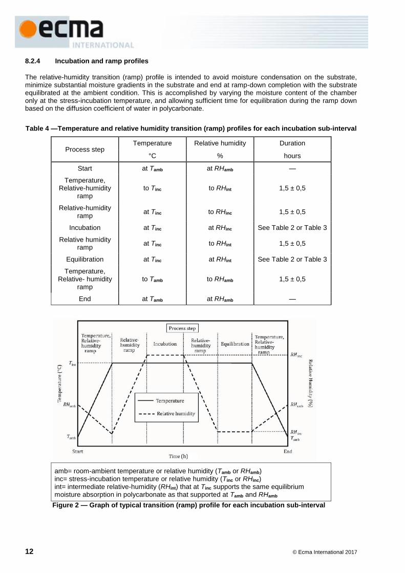
8.2.4 Incubation and ramp profiles
The relative-humidity transition (ramp) profile is intended to avoid moisture condensation on the substrate, minimize substantial moisture gradients in the substrate and end at ramp-down completion with the substrate equilibrated at the ambient condition. This is accomplished by varying the moisture content of the chamber only at the stress-incubation temperature, and allowing sufficient time for equilibration during the ramp down based on the diffusion coefficient of water in polycarbonate.
Table 4 —Temperature and relative humidity transition (ramp) profiles for each incubation sub-interval
Process step Temperature Relative humidity Duration
°C % hours
Start at Tamb at RHamb —
Temperature, Relative-humidity
ramp to Tinc to RHint 1,5 ± 0,5
Relative-humidity ramp
at Tinc to RHinc 1,5 ± 0,5
Incubation at Tinc at RHinc See Table 2 or Table 3
Relative humidity ramp
at Tinc to RHint 1,5 ± 0,5
Equilibration at Tinc at RHint See Table 2 or Table 3
Temperature, Relative- humidity
ramp to Tamb to RHamb 1,5 ± 0,5
End at Tamb at RHamb —
amb= room-ambient temperature or relative humidity (Tamb or RHamb) inc= stress-incubation temperature or relative humidity (Tinc or RHinc) int= intermediate relative-humidity (RHint) that at Tinc supports the same equilibrium moisture absorption in polycarbonate as that supported at Tamb and RHamb
Figure 2 — Graph of typical transition (ramp) profile for each incubation sub-interval

© Ecma International 2017 13
8.3 Measuring-time intervals
For data collection, RSER (BD Recordable SL/DL disk, BD Recordable TL/QL disk, BD Rewritable SL/DL disk, BD Rewritable TL disk), PI Sum 8 (DVD-R, DVD-RW, +R, +RW disk), BER (DVD-RAM disk), or C1 Ave 10 (CD-R, CD-RW disk) shall be measured on each disk : 1) before disk exposure to any stress condition to determine its baseline measurement and 2) after each incubation sub-interval. The length of time for intervals is dependent on the severity of the stress conditions.
In case all the data errors of specimens do not reach the failure criteria (see 9.1) within the minimum total incubation time, testing at a particular stress condition may have to be stopped (see A.2.1 for guidance).
8.4 Design of stress conditions
A separate group of specimens shall be used for each stress condition.
Table 2, for the Rigorous stress-condition, and Table 3, for the Basic stress-condition, specify the temperatures, relative-humidity values, maximum Incubation sub-intervals, minimum total incubation time, and minimum number of specimens for each stress condition. All temperatures shall be maintained within ± 2 °C of the target temperature; all relative-humidity values shall be maintained within ± 3 % RH of the target relative humidity.
The intermediate relative-humidity values in Table 2 and Table 3 are calculated assuming 25 °C and 50 % RH ambient conditions. If the ambient is different, the intermediate relative humidity to be used is calculated using the equation:
ambinc
ambint
7003,024,0
7003,024,0RH
T
TRH
where,
Tamb and Tinc are the ambient and incubation temperature in units of °C,
RHamb is the ambient relative humidity,
RHint is the intermediate relative humidity.
The stress conditions in Table 2, Table 3 and Table 4 offer sufficient combinations of temperature and relative humidity to satisfy the mathematical requirements of the Eyring method.
8.5 Disk orientation
The disks subjected to this test method shall be maintained during incubation in a vertical position with a minimum of 2 mm separation between disks to allow air flow between disks and to minimize deposition of debris, which could negatively influence the data-error measurements, on the disk surface.
9 Lifetime estimation
9.1 Time-to-failure
Ideally, all disks subjected to stress conditions should have their times-to-failure calculated at the stress conditions they have been subjected to. The time-to-failure of a disk is determined by the test data including the Maximum Data Error (see A.2.1). In case any times-to-failures are not available for a stress condition, however, see A.2.3.
Failure criteria are: Max RSER exceeding 10-3 for BD Recordable SL/DL disks, BD Recordable TL/QL disks, BD Rewritable SL/DL disks and BD Rewritable TL disks (see Annex F), Max PI Sum 8 exceeding 280 for

14 © Ecma International 2017
DVD-R/RW disks and +R/+RW disks, Max BER exceeding 10-3 for DVD-RAM disks and Max C1 Ave 10 exceeding 220 for CD-R/RW disks.
It is assumed that the data errors on a disk are the result of material degradation. The chemical changes are generally expected to cause test data to have a distribution that follows an exponential function over time. Therefore, test values of: PI Sum 8, BER, C1 Ave 10 or RSER as functions of time are expected to exhibit an exponential distribution.
The best function fitting an error trend can be found by regression of the test data against time, for example, with a least-squares fit. The time-to-failure per disk type can be calculated using the error-trend function and the failure criteria. But if a determination of time-to-failure is judged not to be effective then that case should be treated as a missing time-to-failure (see A.2.1).
9.2 Accelerated-aging test methods
9.2.1 Eyring acceleration model (Eyring method)
Using the Eyring model, the following equation is derived from the laws of thermodynamics and can be used to handle the two critical stresses of temperature and relative humidity.
RHTkTH eeTt )/CB(/aA
where
t is the time to failure, A is the pre-exponential time constant,
aT is the pre-exponential temperature factor, ΔH is the activation energy per molecule, k is the Boltzmann's constant (1,380 7 × 10-23 J/molecule degree K), T is the temperature (in Kelvin), B, C are the RH exponential constants, In this Ecma Standard T (in Kelvin) is set as T = 273,15+Temp (°C).
For the temperature range used in this test method, “a” and “C” shall be set to zero. The Eyring-model equation then reduces to the following equation:
RHkTH eet B/A
or, RHkT
Ht
B)A(ln)(ln .
9.2.2 Arrhenius accelerated model (Arrhenius method)
The Arrhenius method uses only temperature stress for accelerated aging.
The time-to-failure is assumed to be governed by the following Arrhenius-model equation:
kTHet /A ,
kT
Ht
)A(ln)(ln .
9.3 Data analysis and judgment of effectiveness
Data analysis and a method for judging the effectiveness of the data are contained in the following Annexes:
© Ecma International 2017 15
Annex A: Outline of Disk-life estimation method and data-analysis steps,
Annex B: Disk-life estimation for the Controlled storage-condition (Eyring method),
Annex C: Disk-life estimation for the Harsh storage-condition (Arrhenius method),
Annex E: Interval estimation for B5 Life using maximum likelihood.
9.4 Result of estimated disk life
An estimated lifetime based on the data analysis shall be reported as follows.
(a) Number and title of this standard.
(b) Ambient storage-condition for the lifetime estimation:
25 °C / 50 % RH (Controlled storage-condition) or 30 °C / 80 % RH (Harsh storage-condition).
(c) Disk testing location:
Rigorous testing location or Basic testing location (see 7.5).
(d) Stress and testing condition:
Rigorous stress-condition testing or Basic stress-condition testing and whether or not the alternative condition was used.
(e) The recording speed used for testing shall be reported (see 7.3).
(f) Time-to-failure data
Complete data or data with the substitutes of missing times-to-failure.
(g) Sample information
Number of samples tested under each stress condition.
(h) Estimation method and the estimated data
Maximum-likelihood method with the least squares method/acceleration-factor method and the estimated log standard deviation
(i) B50 Life, B5 Life and 95 % lower confidence bound of B5 Life (= (B5 Life)L) for the maximum-likelihood method with least squares method.
B50 Life, B5 Life and the point estimates of the 5 percentile with variation (= B5V Life) for the acceleration-factor method.

16 © Ecma International 2017

© Ecma International 2017 17
Annex A (normative)
Outline of Disk-life estimation method and data-analysis steps
A.1 Data analysis for Disk-life estimation
A.1.1 General
Data analysis for lifetime estimation is based on the following assumptions.
- The lifetime of data recorded on an optical disk has a lognormal distribution.
- The Eyring method is used for the Controlled storage condition (25 °C, 50 % RH) (see Annex B).
- The Arrhenius method is used for the Harsh storage condition (30 °C, 80 % RH) (see Annex C).
The maximum-likelihood method (see Annex E) is applied for a precise analysis and a precise interval estimation. Thus the lifetime estimation in this Ecma Standard is specified based on the maximum-likelihood method estimation.
The calculation for the maximum-likelihood method is complicated and it is not so easy to adopt. If the lifetime data is complete and its distribution is lognormal, then the estimated lifetime can also be calculated using the least-squares method and the calculated results will be the same as that of the maximum-likelihood method. Thus for the complete data case the least-squares method, which is relatively easy to calculate, is adopted as the practical calculation method for estimating the population.
For the case that the lifetime data is not complete and there are missing times-to-failure, the estimation method is shown in A.2.4 as an informative sub clause.
The acceleration-factor method has been widely used for the lifetime estimation of DVD disks. Those who need the evaluation with relation to the past data can refer to the acceleration method, explained in A.2.6 and B.3.
There can be the case of the multi-layer disk that the Maximum Data Error occurs in different layers after each incubation sub-interval time according to the acceleration condition. In that case at first it is recommended to confirm that there is not any abnormal Maximum Data Error value. In such a case the time-to-failure of multi-layer disk should be estimated for each layer and the time-to-failure of the disk should be the minimum one among the layers.
A.1.2 Lognormal model and point estimation of 5ˆlnB and 50
ˆlnB
As time-to-failure t is distributed with lognormal distribution ),( 2σμLN , log lifetime ( ty ln ) follows a normal
distribution ),( 2σμN , where μ and 2σ are the expected values of y and variance, respectively. μ can be
expressed as a function of x as follows,
zσμy )(x
zσxβxββ 22110
NOTE x is a vector with two dimensions (x1, x2).

18 © Ecma International 2017
where z denotes a percentile of N(0,1), β0 = ln A, β1 = ΔH /k, β2 = B (for the definition of A and B see 9.2.1), x1 represents the variable related to the temperature as x1 = 1/T and x2 represents the variable related to the relative humidity as x2 = RH .
The p percentile of the lifetime distribution, or BP Life, is widely used in reliability engineering. The point
estimation of pBln is described as
σzxβxββB ˆˆˆˆˆln 100/p22110p .
Then the point estimates of the 5 percentile and 50 percentile of the lifetime distribution are given by:
σ,xβxββB ˆ641ˆˆˆˆln 20210105 ,
202101050ˆˆˆˆln xβxββB .
where, 2010,xx denotes the Controlled storage-condition ( 25 °C and 50 % RH ).
(x10 = 1/(273,15 + 25) , x20 = 50 )
NOTE The purpose of the lifetime estimation is to estimate the lifetime of the population. Thus 2 is the unbiased
variance.
A.1.3 Interval estimation for optical disks
For interval estimation of pBln for an optical disk, one may consider only the lower bound.
%)100( α lower confidence bound of log lifetime pBln is given by the following equation:
)ˆvar(lnˆln)ˆln( 100/L pαpp BzBB ,
where, )ˆln(var pB denotes the variance of pBln (see Annex E).
A.1.4 Estimation of β and σ using least-squares method
The multiple linear-regression model for the i j th specimen is described as follows.
)to1()to1(22110 Jjniεxβxββy jijjjij ,
where, i jε denotes errors, nj denotes the number of specimens in each group and J denotes the
total number of groups.
The estimate jy is given as
jjj xβxββy 22110ˆˆˆˆ ,
where, x1j = 1/(273,15 + Tj (in °C) x2j = RHj.
Also, the sum of squared residual errors eS is computed as
2
11
)ˆ( j
n
iij
J
je yyS
j
.
© Ecma International 2017 19
If the lifetime data is complete and the distribution is lognormal then the estimated regression coefficients obtained by the least-squares method are the same as that of the maximum-likelihood method and they can be used for the estimation. The following shows the way to utilize the calculation results obtained by the least-squares method.
The estimated regression coefficients of jy can be obtained by applying the least-squares method to eS . The
estimates 210ˆandˆ,ˆ βββ are obtained by solving 110 linear-regression equations of group A, B, C, D and E.
Let 2ˆlsmσ be the unbiased variance obtained by the least-squares method, then
the estimate 2ˆlsmσ is given by
)3(
)ˆ(
)3(ˆ 1 1
2
2
n
yy
n
Sσ
J
j
n
i
jij
elsm
j
where, n =
J
jjn
1
and it denotes the total number of specimens.
3n 12n . -1 is for the limited number of the sampling and -2 is for the number of degrees of freedom
(temperature and humidity).
NOTE This clause shows the case for the Eyring method. In case of the Arrhenius method the degree of freedom is 1
(temperature only) and n -3 becomes n-2.
The estimated regression-coefficients 10ˆ,ˆ ββ and 2β and estimated variance of residual errors 2ˆ
lsmσ are
obtained using regression analysis statistics software tools.
B50 Life, B5 Life and the 95 % lower confidence bound of B5 Life are described as follows.
B50 Life = )ˆln(exp 50B
= exp ( 2021010ˆˆˆ xβxββ ),
B5 Life = )ˆln(exp 5B
= exp ( σxβxββ ˆ64,1ˆˆˆ2021010 ),
= exp ( lsmσxβxββ ˆ64,1ˆˆˆ2021010 ),
where, 2010,xx denotes the Controlled storage-condition ( 25 °C and 50 % RH ).
By substitutinglsm
σ for σ , )ˆln(var50
B and )ˆln(var5
B are obtained as follows (see E.3).
20
10
2
2
1
221
1
2
1
22
21
1
2
2
1
1
2
1
12
1
22
1
122
201050
1
ˆ
1
ˆ
1
ˆ
1
ˆ
1
ˆ
1
ˆ
1
ˆ
1
ˆ
1
ˆ
1)ˆln(var
1
x
x
xnσ
xxnσ
xnσ
xxnσ
xnσ
xnσ
xnσ
xnσσ
n
xxB
j
J
j
j
lsm
jj
J
j
j
lsm
J
j
jj
lsm
jj
J
j
j
lsm
j
J
j
j
lsm
J
j
jj
lsm
J
j
jj
lsm
J
j
jj
lsmlsm
20 © Ecma International 2017
64,1
1
ˆ
2000
0ˆ
1
ˆ
1
ˆ
1
0ˆ
1
ˆ
1
ˆ
1
0ˆ
1
ˆ
1
ˆ
64,11)ˆln(var20
10
2
2
2
1
221
1
2
1
22
21
1
2
2
1
1
2
1
12
1
22
1
122
20105
1
x
x
σ
n
xnσ
xxnσ
xnσ
xxnσ
xnσ
xnσ
xnσ
xnσσ
n
xxB
lsm
j
J
j
j
lsm
jj
J
j
j
lsm
J
j
jj
lsm
jj
J
j
j
lsm
j
J
j
j
lsm
J
j
jj
lsm
J
j
jj
lsm
J
j
jj
lsmlsm
where, n =
J
jjn
1
and it denotes the total number of specimens.
Using the result of the above equation, the lower confidence bound of log lifetime 5
ˆlnB = (B5 Life)L is given by
the following equation.
(B5 Life)L ))ˆvar(ln64,1ˆln(exp))ˆln((exp 55L5 BBB
A.2 Data analysis steps for lifetime estimation
A.2.1 Judgment of effectiveness of test data and time-to-failure determination
Before the lifetime-estimation calculation, the effectiveness of the test data shall be checked, following the procedure listed below.
Step 1:
Calculate the linear regression or the polynomial regression of the logarithm of test-data error rate (Errort) = ln(Errort) against incubation time and plot ln(Errort) versus the incubation time and their best-fit line on the linear-scale graph for each test-condition specimen.
Step 2:
Check the following three conditions:
a) The best-fit line increases monotonously.
b) All ln(Errort) are almost on the best-fit line.
c) The best-fit line has reasonable increase and is not flat nor having a negative slope.
If all three conditions are satisfied, then go to Step 3.
If the three conditions are not satisfied, then that time-to-failure shall not be determined.
There are two cases where the above three conditions are not satisfied.
- The first case is that there is a sample that shows unexpected deterioration during the first sub-interval time of the accelerated-aging test while other samples satisfy the three conditions. In this case the deterioration mechanism of the abnormal sample can be different from that of other samples. The sample whose error rate cannot be obtained after the first sub-interval time shall
© Ecma International 2017 21
be treated as having the missing time-to-failure. Then go to Step 4 in A.2.2. In this case keep the number of specimens as it is.
- The second case is that there is a sample in a group which does not deteriorate within the minimum total incubation-time and its best-fit line does not show reasonable increase while other samples in that group satisfy the three conditions. The case when the time-to-failure of a sample that does not satisfy the three conditions shall be treated as the missing time-to-failure and the procedure shall continue at Step 4 in A.2.2. In this case keep the number of specimens as it is.
If there are some ln(Errort)s that show abnormal values, it is recommended to check the reason why those values are abnormal, if possible, and it is also recommended to judge whether to adopt those values or not.
Step 3:
For each test-condition specimen, determine the time-to-failure where the best-fit line crosses the failure criteria.
For a test-condition specimen for which the measured error rate did not reach the failure criteria within the minimum total incubation-time, the time-to-failure may be determined using the extrapolation of the best-fit line of ln(Errort) as a predicted time-to-failure.
After Step 3, go to the procedure in A.2.2.
A.2.2 Judgment of complete data
Follow the procedure listed below.
Step 4:
For each specimen of a stress group, order the time-to-failure values by increasing incubation time. Calculate the median rank of each specimen for each time-to-failure (see B.1 Step 2).
If there is a sample that shows unexpected deterioration during the first sub-interval time of the accelerated-aging then its missing time-to-failure shall be given the median rank smaller than that of the shortest time-to-failure when sorting times-to-failure for the determination of the median rank.
If there is a sample that does not deteriorate within the minimum total incubation-time then its missing time-to-failure shall be given the median rank larger than that of the longest time-to-failure when sorting times-to-failure for the determination of the median rank.
Step 5:
Plot the median rank versus the time-to-failure on a lognormal graph, with time-to-failure on the abscissa and median rank on the ordinate, for each specimen of the stress group.
Plot the best-fit straight line for each specimen of the stress group.
Step 6:
Check the following conditions.
a) All the times-to-failure corresponding to each median rank are almost on the best-fit straight-line of each stress group.
b) The best-fit straight lines of all stress groups are reasonably parallel with each other.
If both conditions listed above are satisfied, then the data is deemed complete. Proceed to the procedure in A.2.5 (Maximum-likelihood method with least-squares method) or in A.2.6 (acceleration-
22 © Ecma International 2017
factor method). For the precise analysis or the precise interval estimation, go to the procedure in A.2.5.
If a time-to-failure is away from the best-fit straight line, then that time-to-failure shall not be used for the lifetime estimation. That time-to-failure is treated as a missing time-to-failure.
If at least one condition listed above is not satisfied, then go to the procedure in A.2.3.
A.2.3 Condition for lifetime-estimation effectiveness
Follow the procedure listed below.
Step 7:
Check the following three conditions and judge the effectiveness of the time-to-failure.
a) The lognormal data plots of each stress group are almost on the best-fit straight-line.
b) Exclude the missing times-to-failure, then check the specimens of each stress group have effective times-to-failure that span over one-half of a median rank point.
c) The best-fit straight lines of all stress groups are reasonably parallel with one another.
If these three conditions are satisfied, we can assume that the lifetime distribution is lognormal. In case there are missing times-to-failure the calculation based on the maximum-likelihood method can be possible, but the method is complicated and is not easy to apply. There is a possibility that it is not as precise as the maximum-likelihood method but the other method in which the missing times-to-failure are substituted is shown in A.2.4.
In A.1, it was assumed that the lifetime data has a lognormal distribution. If the three conditions are not satisfied, it is proven that the assumption is not effective and a reliable lifetime estimation cannot be obtained.
A.2.4 Life-time estimation when there are missing times-to-failure (Informative)
As shown in Step 7 in A.2.3 there are cases that lifetime distribution is lognormal but missing times-to-failure exist. The method to substitute those missing times-to-failure is shown in this clause. Be aware that this method uses substituted data in the best-fit straight lines and the estimated lifetime may be longer.
a) Substitution of times-to-failure
For each missing time-to-failure, check the corresponding median rank and substitute the missing time-to-failure value with the value where the best-fit straight line crosses the corresponding median rank on the lognormal graph.
b) Maximum-likelihood method with least-squares method application
Substitute all the missing times-to-failure and prepare the complete data set. Then follow the steps in A.2.5.
c) Acceleration-factor method application
Substitute all the missing times-to-failure and prepare the complete data set. Then follow the steps in A.2.6. For the precise analysis or the precise interval estimation, go to the steps in A.2.5.
© Ecma International 2017 23
A.2.5 Lifetime-estimation calculation method (Maximum-likelihood method with least-squares method)
Calculation of the maximum likelihood method with the least-squares method can be done as listed below.
a) Calculate the multiple regression coefficients and standard error using the least-squares method across all times-to-failure. This calculation can be performed by multiple regression analysis using statistics software tools.
The coefficient of determination is expected to be over 0,8. If the coefficient of determination of the multiple regression analysis is too small then it is recommended to reconsider the accelerated aging-test condition.
b) B50 Life, B5 Life and 95 % lower confidence bound of B5 Life at the Controlled storage condition are calculated using the multiple regression-coefficients and standard error obtained by the least-squares method and the equations of maximum-likelihood method (see B.33 and E.4).
A.2.6 Lifetime-estimation calculation method (acceleration-factor method)
Calculation of the conventional acceleration-factor method can be done as follows.
a) Calculate regression coefficients using the log-mean failure time.
b) Calculate acceleration factors from the difference between the estimated log-mean at each stress condition.
c) Calculate the normalized time-to-failure at the ambient condition for each specimen group using the acceleration factors, and plot these data on a lognormal graph.
d) Assuming that the normal distribution of the population varies according to the 95% lower confidence bound of the normal distribution, B50 Life, B5 Life and the point estimates of the percentile with variation
(= B5V Life) at the Controlled storage-condition are calculated using σμ ˆandˆ obtained from the fitting
line (see B.33).
NOTE The data-analysis steps using the Arrhenius method are almost the same as with the Eyring method. A single
regression at the Harsh storage temperature can be used with the Arrhenius method.

24 © Ecma International 2017
© Ecma International 2017 25
Annex B (normative)
Disk-life estimation for Controlled storage-condition
(Eyring method)
B.1 General
In this annex, the analysis of the complete data case using the results of a least-squares method and a conventional acceleration-factor method for the Rigorous stress-condition testing are shown.
B.2 Data analysis and lifetime estimation using least-squares method
Step 1
Determine the time-to-failure for each specimen at the stress applied following the procedure described below. The data error to be measured is defined in 7.1.3:
BD Recordable disks and BD Rewritable disks: Max RSER, DVD-R/RW, +R/+RW disks: Max PI Sum 8,
DVD-RAM disks: Max BER, CD-R/RW disks: Max C1 Ave 10.
Use the initial data-errors measured prior to accelerated aging plus the data errors measured after each specified accelerated-aging incubation sub-interval.
For each specimen, a linear regression is performed with the natural logarithm of measured data-errors as the dependent variable and time as the independent variable. The time-to-failure of the specimen is calculated from the slope and intercept of the regression as the time at which the specimen would have a Max RSER of 10-3, Max PI Sum 8 of 280, Max BER of 10-3 or Max C1 Ave 10 of 220.
Table B.1 shows calculations leading to an estimated time-to-failure from a hypothetical data set. The data for five stress conditions (Group A, Group B, Group C, Group D and Group E) are offered solely as an example of the mathematical methodology used in this test procedure.
Step 2
For each stress condition, the specimens are ordered by increasing log time-to-failure values.
The median rank of each specimen is calculated using the estimate )4,0/()3,0( ni , where i is the time-to-
failure order and n is the total number of specimens at the stress condition.
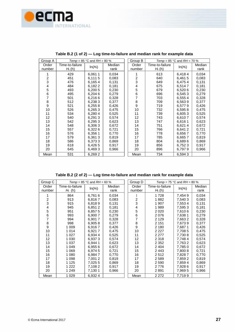
Table B.2 shows the ordered log time-to-failure and the median rank for the example data.
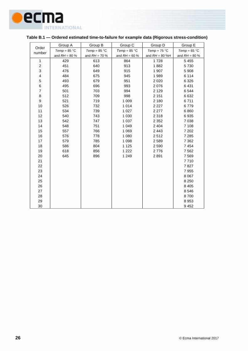
26 © Ecma International 2017
Table B.1 — Ordered estimated time-to-failure for example data (Rigorous stress-condition)
Order
number
Group A Group B Group C Group D Group E
Temp = 85 °C
and RH = 80 %
Temp = 85 °C
and RH = 70 %
Temp = 85 °C
and RH = 60 %
Temp = 75 °C
and RH = 80 %H
Temp = 65 °C
and RH = 80 %
1
2
3
4
5
6
7
8
9
10
11
12
13
14
15
16
17
18
19
20
21
22
23
24
25
26
27
28
29
30
429
451
476
484
493
495
501
512
521
526
534
540
542
548
557
576
579
586
618
645
613
640
649
675
679
696
703
709
719
732
739
743
747
751
766
778
785
804
856
896
864
913
915
945
951
993
994
998
1 009
1 014
1 027
1 030
1 037
1 049
1 069
1 080
1 098
1 125
1 222
1 249
1 728
1 882
1 907
1 989
2 020
2 076
2 129
2 151
2 180
2 227
2 277
2 318
2 352
2 404
2 443
2 512
2 589
2 590
2 776
2 891
5 455
5 730
5 908
6 114
6 326
6 431
6 544
6 632
6 711
6 779
6 860
6 935
7 038
7 108
7 202
7 285
7 362
7 454
7 562
7 569
7 710
7 827
7 955
8 067
8 250
8 405
8 546
8 700
8 953
9 452
© Ecma International 2017 27
Table B.2 (1 of 2) — Log time-to-failure and median rank for example data
Group A Temp = 85 °C and RH = 80 % Group B Temp = 85 °C and RH = 70 %
Order number
Time-to-failure Ht (h)
ln(Ht) Median
rank Order
number Time-to-failure
Ht (h) ln(Ht)
Median rank
1 2 3 4 5 6 7 8 9 10 11 12 13 14 15 16 17 18 19 20
429 451 476 484 493 495 501 512 521 526 534 540 542 548 557 576 579 586 618 645
6,061 1 6,111 5 6,165 4 6,182 2 6,200 5 6,204 6 6,216 6 6,238 3 6,255 8 6,265 3 6,280 4 6,291 3 6,295 3 6,306 3 6,322 6 6,356 1 6,361 3 6,373 3 6,426 5 6,469 3
0,034 0,083 0,131 0,181 0,230 0,279 0,328 0,377 0,426 0,475 0,525 0,574 0,623 0,672 0,721 0,770 0,819 0,869 0,917 0,966
1 2 3 4 5 6 7 8 9 10 11 12 13 14 15 16 17 18 19 20
613 640 649 675 679 696 703 709 719 732 739 743 747 751 766 778 785 804 856 896
6,418 4 6,461 5 6,475 4 6,514 7 6,520 6 6,545 3 6,555 4 6,563 9 6,577 9 6,595 8 6,605 3 6,610 7 6,616 1 6,621 4 6,641 2 6,656 7 6,665 7 6,689 6 6,752 3 6,797 9
0,034 0,083 0,131 0,181 0,230 0,279 0,328 0,377 0,426 0,475 0,525 0,574 0,623 0,672 0,721 0,770 0,819 0,869 0,917 0,966
Mean 531 6,269 2 Mean 734 6,594 3
Table B.2 (2 of 2) — Log time-to-failure and median rank for example data
Group C Temp = 85 °C and RH = 60 % Group D Temp = 75 °C and RH = 80 %
Order number
Time-to-failure Ht (h)
ln(Ht) Median
rank
Order number
Time-to-failure Ht (h)
ln(Ht) Median
rank
1 2 3 4 5 6 7 8 9 10 11 12 13 14 15 16 17 18 19 20
864 913 915 945 951 993 994 998
1 009 1 014 1 027 1 030 1 037 1 049 1 069 1 080 1 098 1 125 1 222 1 249
6,761 6 6,816 7 6,818 9 6,851 2 6,857 5 6,900 7 6,901 7 6,905 8 6,916 7 6,921 7 6,934 4 6,937 3 6,944 1 6,955 6 6,974 5 6,984 7 7,001 2 7,025 5 7,108 2 7,130 1
0,034 0,083 0,131 0,181 0,230 0,279 0,328 0,377 0,426 0,475 0,525 0,574 0,623 0,672 0,721 0,770 0,819 0,869 0,917 0,966
1 2 3 4 5 6 7 8 9 10 11 12 13 14 15 16 17 18 19 20
1 728 1 882 1 907 1 989 2 020 2 076 2 129 2 151 2 180 2 227 2 277 2 318 2 352 2 404 2 443 2 512 2 589 2 590 2 776 2 891
7,454 9 7,540 3 7,553 4 7,595 3 7,610 6 7,638 1 7,663 2 7,673 9 7,687 1 7,708 5 7,730 8 7,748 4 7,763 2 7,785 0 7,800 8 7,828 7 7,859 2 7,859 4 7,928 6 7,969 5
0,034 0,083 0,131 0,181 0,230 0,279 0,328 0,377 0,426 0,475 0,525 0,574 0,623 0,672 0,721 0,770 0,819 0,869 0,917 0,966
Mean 1 029 6,932 4 Mean 2 272 7,719 9
28 © Ecma International 2017
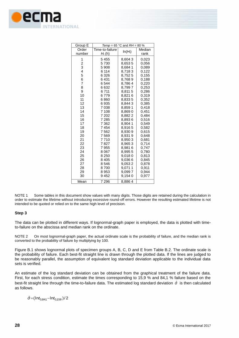
Group E Temp = 65 °C and RH = 80 %
Order number
Time-to-failure Ht (h)
ln(Ht) Median
rank
1 2 3 4 5 6 7 8 9 10 11 12 13 14 15 16 17 18 19 20 21 22 23 24 25 26 27 28 29 30
5 455 5 730 5 908 6 114 6 326 6 431 6 544 6 632 6 711 6 779 6 860 6 935 7 038 7 108 7 202 7 285 7 362 7 454 7 562 7 569 7 710 7 827 7 955 8 067 8 250 8 405 8 546 8 700 8 953 9 452
8,604 3 8,653 5 8,684 1 8,718 3 8,752 5 8,768 9 8,786 4 8,799 7 8,811 5 8,821 6 8,833 5 8,844 3 8,859 1 8,869 0 8,882 2 8,893 6 8,904 1 8,916 5 8,930 9 8,931 9 8,950 3 8,965 3 8,981 6 8,995 5 9,018 0 9,036 6 9,053 2 9,071 1 9,099 7 9,154 0
0,023 0,056 0,089 0,122 0,155 0,188 0,220 0,253 0,286 0,319 0,352 0,385 0,418 0,451 0,484 0,516 0,549 0,582 0,615 0,648 0,681 0,714 0,747 0,780 0,813 0,845 0,878 0,911 0,944 0,977
Mean 7 296 8,886 4
NOTE 1 Some tables in this document show values with many digits. Those digits are retained during the calculation in order to estimate the lifetime without introducing excessive round-off errors. However the resulting estimated lifetime is not
intended to be quoted or relied on to the same high level of precision.
Step 3
The data can be plotted in different ways. If lognormal-graph paper is employed, the data is plotted with time-to-failure on the abscissa and median rank on the ordinate.
NOTE 2 On most lognormal-graph paper, the actual ordinate scale is the probability of failure, and the median rank is converted to the probability of failure by multiplying by 100.
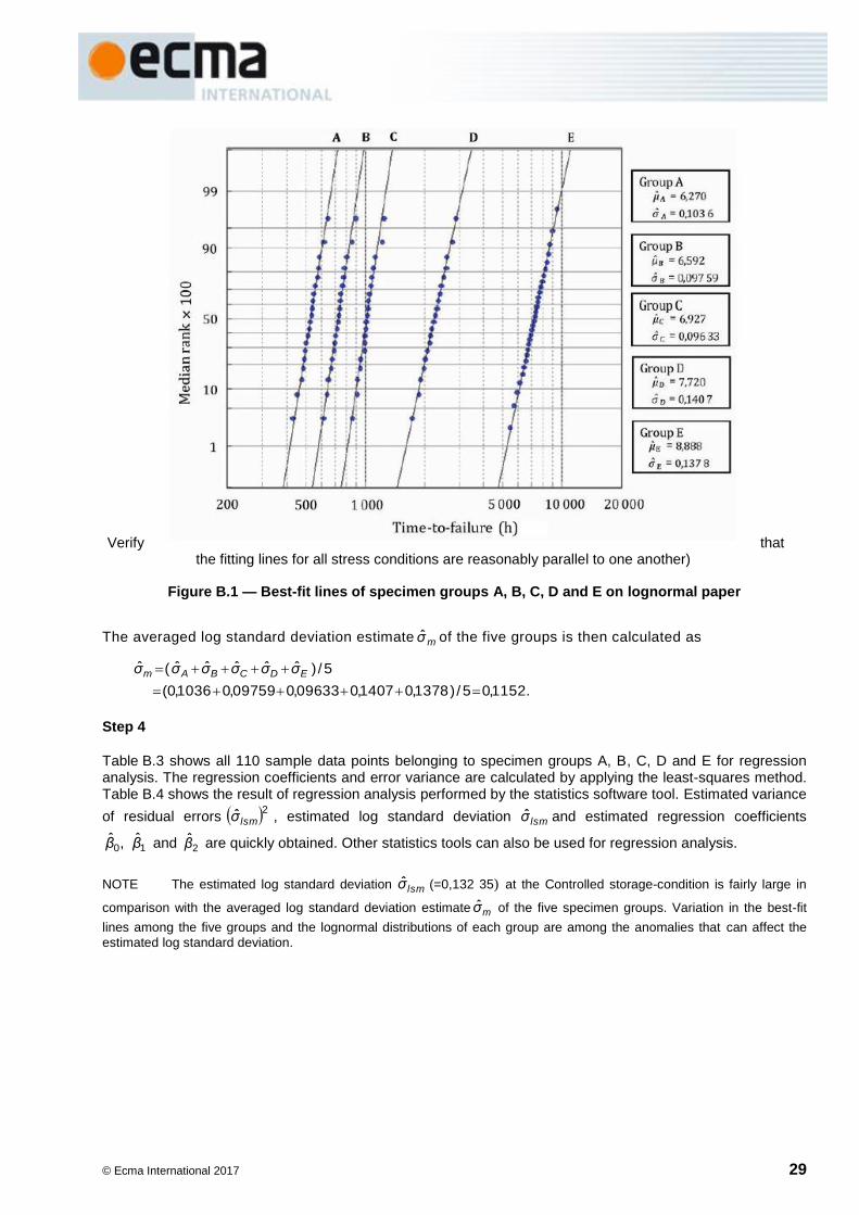
Figure B.1 shows lognormal plots of specimen groups A, B, C, D and E from Table B.2. The ordinate scale is the probability of failure. Each best-fit straight line is drawn through the plotted data. If the lines are judged to be reasonably parallel, the assumption of equivalent log standard deviation applicable to the individual data sets is verified.
An estimate of the log standard deviation can be obtained from the graphical treatment of the failure data. First, for each stress condition, estimate the times corresponding to 15,9 % and 84,1 % failure based on the
best-fit straight line through the time-to-failure data. The estimated log standard deviation σ is then calculated
as follows.
2/)lnln(ˆ159,0841,0 ttσ
© Ecma International 2017 29
Verify that the fitting lines for all stress conditions are reasonably parallel to one another)
Figure B.1 — Best-fit lines of specimen groups A, B, C, D and E on lognormal paper
The averaged log standard deviation estimate mσ of the five groups is then calculated as
.2115,05/)8137,07140,033096,059097,06103,0(
5/)ˆˆˆˆˆ(ˆ
EDCBAm σσσσσσ
Step 4
Table B.3 shows all 110 sample data points belonging to specimen groups A, B, C, D and E for regression analysis. The regression coefficients and error variance are calculated by applying the least-squares method. Table B.4 shows the result of regression analysis performed by the statistics software tool. Estimated variance
of residual errors 2ˆlsmσ , estimated log standard deviation lsmσ and estimated regression coefficients
10ˆ,ˆ ββ and 2β are quickly obtained. Other statistics tools can also be used for regression analysis.
NOTE The estimated log standard deviation lsmσ (=0,132 35) at the Controlled storage-condition is fairly large in
comparison with the averaged log standard deviation estimate mσ of the five specimen groups. Variation in the best-fit
lines among the five groups and the lognormal distributions of each group are among the anomalies that can affect the
estimated log standard deviation.
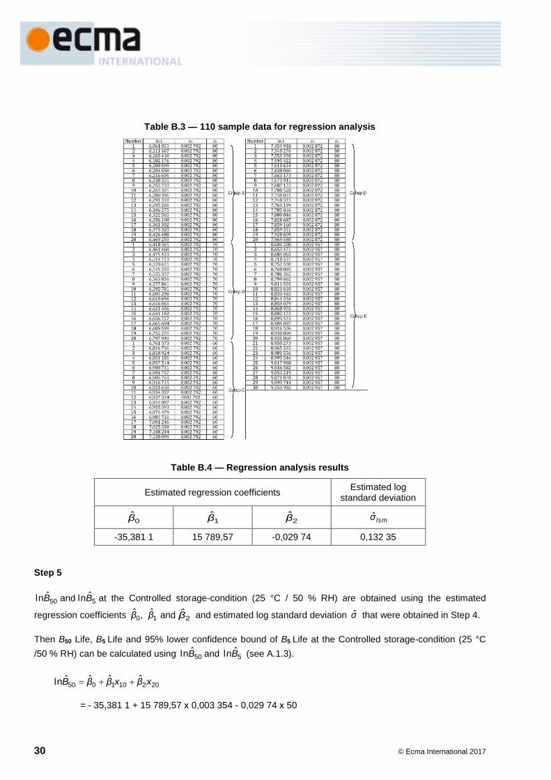
30 © Ecma International 2017
Table B.3 — 110 sample data for regression analysis
Table B.4 — Regression analysis results
Estimated regression coefficients Estimated log
standard deviation
0β 1β 2β lsmσ
-35,381 1 15 789,57 -0,029 74 0,132 35
Step 5
50ˆlnB and 5
ˆlnB at the Controlled storage-condition (25 °C / 50 % RH) are obtained using the estimated
regression coefficients 10ˆ,ˆ ββ and 2β and estimated log standard deviation σ that were obtained in Step 4.
Then B50 Life, B5 Life and 95% lower confidence bound of B5 Life at the Controlled storage-condition (25 °C
/50 % RH) can be calculated using 50ˆlnB and 5
ˆlnB (see A.1.3).
202101050ˆˆˆˆln xβxββB
= - 35,381 1 + 15 789,57 х 0,003 354 - 0,029 74 х 50

© Ecma International 2017 31
= 16,090 1.
B50 Life = exp (16,090 1) = 9 724 120 hours (1 110 years).,
lsmσBσxβxββB ˆ64,1ˆlnˆ64,1ˆˆˆˆln 5020210105
= 16,090 1 – 1,64 х 0,132 35
= 15,873 0
B5 Life = exp (15,873 0) = 7 826 297 hours (893 years).
The 95% lower confidence bound of B5 Life is therefore
(B5 Life)L ))ˆvar(ln64,1ˆ(lnexp))ˆvar(lnˆ(lnexp))ˆ(lnexp(555100/55L5
BBBzBB
= exp (15,873 0 – 1,64 х 129021,0 ) = exp (15,634 6)
= 6 166 241 hours (704 years) (see E.4).
B.3 Data analysis and lifetime estimation using conventional acceleration-factor method (Step 4-7)
Step 4
Table B.5 shows the average of log time-to-failure for each stress group A, B, C, D, and E (see Table B.2).
Table B.5 — Average log failure time for each stress condition
Group Average Temp
°C 1/T
RH
%
A 6,269 2 85 0,002 792 80
B 6,594 3 85 0,002 792 70
C 6,932 4 85 0,002 792 60
D 7.719 9 75 0,002 872 80
E 8,886 4 65 0,002 957 80
NOTE The average in Table B.5 shows the average value of the ln(Ht)s of each acceleration condition in the mean
row of Table B.2. Instead of such the average value the centre value of the median rank can also be used for log-meani in
the following equation.
To determine the coefficients A, ΔH / k and B of the reduced Eyring equation, regression analysis is done using five average values obtained at the temperature values and relative humidity values in Table B.5 as log-meani.
iii
i εRHTk
Hlog-mean
B)
1()()Aln(
where i = 1 ~ 5.
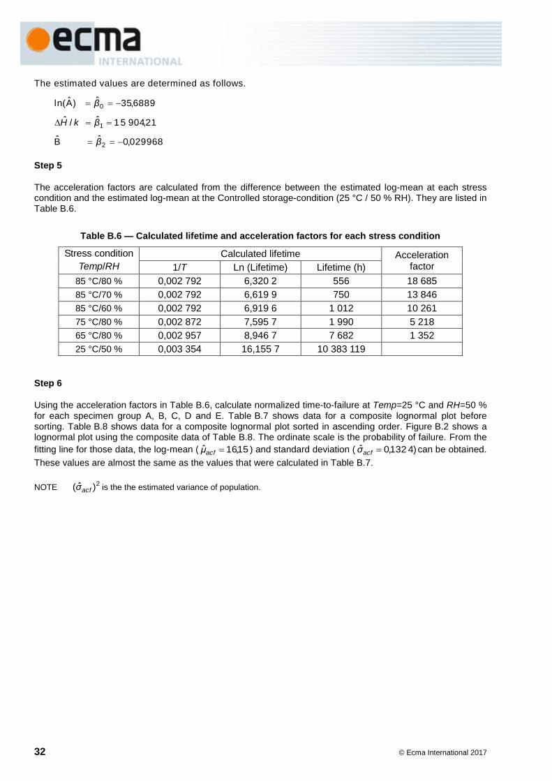
32 © Ecma International 2017
The estimated values are determined as follows.
968029,0ˆB
21,90451ˆ/ˆ
9688,35ˆ)A(ln
2
1
0
β
βkH
β
Step 5
The acceleration factors are calculated from the difference between the estimated log-mean at each stress condition and the estimated log-mean at the Controlled storage-condition (25 °C / 50 % RH). They are listed in Table B.6.
Table B.6 — Calculated lifetime and acceleration factors for each stress condition
Stress condition
Temp/RH
Calculated lifetime Acceleration factor 1/T Ln (Lifetime) Lifetime (h)
85 °C/80 % 0,002 792 6,320 2 556 18 685
85 °C/70 % 0,002 792 6,619 9 750 13 846
85 °C/60 % 0,002 792 6,919 6 1 012 10 261
75 °C/80 % 0,002 872 7,595 7 1 990 5 218
65 °C/80 % 0,002 957 8,946 7 7 682 1 352
25 °C/50 % 0,003 354 16,155 7 10 383 119
Step 6
Using the acceleration factors in Table B.6, calculate normalized time-to-failure at Temp=25 °C and RH=50 % for each specimen group A, B, C, D and E. Table B.7 shows data for a composite lognormal plot before sorting. Table B.8 shows data for a composite lognormal plot sorted in ascending order. Figure B.2 shows a lognormal plot using the composite data of Table B.8. The ordinate scale is the probability of failure. From the
fitting line for those data, the log-mean ( 15,16ˆ acfμ ) and standard deviation ( )4132,0ˆ acfσ can be obtained.
These values are almost the same as the values that were calculated in Table B.7.
NOTE 2)ˆ( acfσ is the the estimated variance of population.

© Ecma International 2017 33
Table B.7 — Data before sorting for composite lognormal plot
Time to Failure
Group Normalized to
Temp = 25 °C
and RH = 50 %
Ln Time to Failure
Group Normalized to
Temp = 25 °C
and RH = 50 %
Ln
429 A 8 015 865 15,896 933 3 1728 D 9 016 704 16,014 589 4
451 A 8 426 935 15,946 943 7 1882 D 9 820 276 16,099 959 8
476 A 8 894 060 16,000 894 2 1907 D 9 950 726 16,113 156 1
484 A 9 043 540 16,017 561 2 1989 D 10 378 602 16,155 256 7
493 A 9 211 705 16,035 985 5 2020 D 10 540 360 16,170 722 3
495 A 9 249 075 16,040 034 1 2076 D 10 832 568 16,198 067 7
501 A 9 361 185 16,052 082 4 2129 D 11 109 122 16,223 277 1
512 A 9 566 720 16,073 801 0 2151 D 11 223 918 16,233 557 6
521 A 9 734 885 16,091 226 4 2180 D 11 375 240 16,246 949 6
526 A 9 828 310 16,100 777 6 2227 D 11 620 486 16,268 280 1
534 A 9 977 790 16,115 872 2 2277 D 11 881 386 16,290 483 5
540 A 10 089 900 16,127 045 5 2318 D 12 095 324 16,308 329 5
542 A 10 127 270 16,130 742 3 2352 D 12 272 736 16,322 890 8
548 A 10 239 380 16,141 751 6 2404 D 12 544 072 16,344 758 8
557 A 10 407 545 16,158 041 6 2443 D 12 747 574 16,360 851 5
576 A 10 762 560 16,191 584 0 2512 D 13 107 616 16,388 704 0
579 A 10 818 615 16,196 778 8 2589 D 13 509 402 16,418 896 4
586 A 10 949 410 16,208 796 1 2590 D 13 514 620 16,419 282 6
618 A 11 547 330 16,261 964 8 2776 D 14 485 168 16,488 635 8
645 A 12 051 825 16,304 726 7 2891 D 15 085 238 16,529 227 2
613 B 8 487 598 15,954 116 6 5455 E 7 375 160 15,813 628 2
640 B 8 861 440 15,997 219 8 5730 E 7 746 960 15,862 811 1
649 B 8 986 054 16,011 184 4 5908 E 7 987 616 15,893 402 9
675 B 9 346 050 16,050 464 4 6114 E 8 266 128 15,927 676 8
679 B 9 401 434 16,056 372 8 6326 E 8 552 752 15,961 763 7
696 B 9 636 816 16,081 101 3 6431 E 8 694 712 15,978 225 6
703 B 9 733 738 16,091 108 6 6544 E 8 847 488 15,995 644 1
709 B 9 816 814 16,099 607 2 6632 E 8 966 464 16,009 002 0
719 B 9 955 274 16,113 613 0 6711 E 9 073 272 16,020 843 5
732 B 10 135 272 16,131 532 2 6779 E 9 165 208 16,030 925 1
739 B 10 232 194 16,141 049 6 6860 E 9 274 720 16,042 803 0
743 B 10 287 578 16,146 447 7 6935 E 9 376 120 16,053 676 6
747 B 10 342 962 16,151 816 8 7038 E 9 515 376 16,068 419 6
751 B 10 398 346 16,157 157 3 7108 E 9 610 016 16,078 316 4
766 B 10 606 036 16,176 933 8 7202 E 9 737 104 16,091 454 3
778 B 10 772 188 16,192 478 2 7285 E 9 849 320 16,102 913 0
785 B 10 869 110 16,201 435 4 7362 E 9 953 424 16,113 427 2
804 B 11 132 184 16,225 350 9 7454 E 10 077 808 16,125 846 3
856 B 11 852 176 16,288 022 0 7562 E 10 223 824 16,140 231 2
896 B 12 406 016 16,333 692 1 7569 E 10 233 288 16,141 156 5
864 C 8 865 504 15,997 678 3 7710 E 10 423 920 16,159 613 7
913 C 9 368 293 16,052 841 5 7827 E 10 582 104 16,174 674 8
915 C 9 388 815 16,055 029 6 7955 E 10 755 160 16,190 896 2
945 C 9 696 645 16,087 290 5 8067 E 10 906 584 16,204 877 2
951 C 9 758 211 16,093 619 6 8250 E 11 154 000 16,227 308 7
993 C 10 189 173 16,136 836 2 8405 E 11 363 560 16,245 922 3

34 © Ecma International 2017
Table B.7 (continued)
Time to Failure
Group Normalized to
Temp = 25 °C
and RH = 50 %
Ln Time to Failure
Group Normalized to
Temp = 25 °C
and RH = 50 %
Ln
994 C 10 199 434 16,137 842 8 8546 E 11 554 192 16,262 558 9
998 C 10 240 478 16,141 858 9 8700 E 11 762 400 16,280 418 6
1009 C 10 353 349 16,152 820 6 8953 E 12 104 456 16,309 084 2
1014 C 10 404 654 16,157 763 8 9452 E 12 779 104 16,363 321 9
1027 C 10 538 047 16,170 502 8 Mean 16,150 284 7
1030 C 10 568 830 16,173 419 7 Deviation 0,130 956 0
1037 C 10 640 657 16,180 192 8
1049 C 10 763 789 16,191 698 2
1069 C 10 969 009 16,210 584 5
1080 C 11 081 880 16,220 821 9
1098 C 11 266 578 16,237 351 2
1125 C 11 543 625 16,261 643 9
1222 C 12 538 942 16,344 349 7
1249 C 12 815 989 16,366 204 1
Table B.8 — Data sorted in ascending order for composite lognormal plot
Group Normalized to
Temp = 25 °C
and RH = 50 %
Order Median
rank Group
Normalized to
Temp = 25 °C
and RH = 50 %
Order Median
rank
E 7 375 160 1 0,006 3 B 10 398 346 61 0,549 8
E 7 746 960 2 0,015 4 C 10 404 654 62 0,558 9
E 7 987 616 3 0,024 5 A 10 407 545 63 0,567 9
A 8 015 865 4 0,033 5 E 10 423 920 64 0,577 0
E 8 266 128 5 0,042 6 C 10 538 047 65 0,586 1
A 8 426 935 6 0,051 6 D 10 540 360 66 0,595 1
B 8 487 598 7 0,060 7 C 10 568 830 67 0,604 2
E 8 552 752 8 0,069 7 E 10 582 104 68 0,613 2
E 8 694 712 9 0,078 8 B 10 606 036 69 0,622 3
E 8 847 488 10 0,087 9 C 10 640 657 70 0,631 3
B 8 861 440 11 0,096 9 E 10 755 160 71 0,640 4
C 8 865 504 12 0,106 0 A 10 762 560 72 0,649 5
A 8 894 060 13 0,115 0 C 10 763 789 73 0,658 5
E 8 966 464 14 0,124 1 B 10 772 188 74 0,667 6
B 8 986 054 15 0,133 2 A 10 818 615 75 0,676 6
D 9 016 704 16 0,142 2 D 10 832 568 76 0,685 7
A 9 043 540 17 0,151 3 B 10 869 110 77 0,694 7
E 9 073 272 18 0,160 3 E 10 906 584 78 0,703 8
E 9 165 208 19 0,169 4 A 10 949 410 79 0,712 9
A 9 211 705 20 0,178 4 C 10 969 009 80 0,721 9
A 9 249 075 21 0,187 5 C 11 081 880 81 0,731 0
E 9 274 720 22 0,196 6 D 11 109 122 82 0,740 0
B 9 346 050 23 0,205 6 B 11 132 184 83 0,749 1
A 9 361 185 24 0,214 7 E 11 154 000 84 0,758 2
C 9 368 293 25 0,223 7 D 11 223 918 85 0,767 2
E 9 376 120 26 0,232 8 C 11 266 578 86 0,776 3
C 9 388 815 27 0,241 8 E 11 363 560 87 0,785 3
B 9 401 434 28 0,250 9 D 11 375 240 88 0,794 4
E 9 515 376 29 0,260 0 C 11 543 625 89 0,803 4
A 9 566 720 30 0,269 0 A 11 547 330 90 0,812 5
E 9 610 016 31 0,278 1 E 11 554 192 91 0,821 6
B 9 636 816 32 0,287 1 D 11 620 486 92 0,830 6
C 9 696 645 33 0,296 2 E 11 762 400 93 0,839 7
B 9 733 738 34 0,305 3 B 11 852 176 94 0,848 7
A 9 734 885 35 0,314 3 D 11 881 386 95 0,857 8
E 9 737 104 36 0,323 4 A 12 051 825 96 0,866 8

© Ecma International 2017 35
Table B.8 (continued)
Group Normalized to
Temp = 25 °C
and RH = 50 %
Order Median
rank Group
Normalized to
Temp = 25 °C
and RH = 50 %
Order Median
rank
C 9 758 211 37 0,332 4 D 12 095 324 97 0,875 9
B 9 816 814 38 0,341 5 E 12 104 456 98 0,885 0
D 9 820 276 39 0,350 5 D 12 272 736 99 0,894 0
A 9 828 310 40 0,359 6 B 12 406 016 100 0,903 1
E 9 849 320 41 0,368 7 C 12 538 942 101 0,912 1
D 9 950 726 42 0,377 7 D 12 544 072 102 0,921 2
E 9 953 424 43 0,386 8 D 12 747 574 103 0,930 3
B 9 955 274 44 0,395 8 E 12 779 104 104 0,939 3
A 9 977 790 45 0,404 9 C 12 815 989 105 0,948 4
E 10 077 808 46 0,413 9 D 13 107 616 106 0,957 4
A 10 089 900 47 0,423 0 D 13 509 402 107 0,966 5
A 10 127 270 48 0,432 1 D 13 514 620 108 0,975 5
B 10 135 272 49 0,441 1 D 14 485 168 109 0,984 6
C 10 189 173 50 0,450 2 D 15 085 238 110 0,993 7
C 10 199 434 51 0,459 2
E 10 223 824 52 0,468 3
B 10 232 194 53 0,477 4
E 10 233 288 54 0,486 4
A 10 239 380 55 0,495 5
C 10 240 478 56 0,504 5
B 10 287 578 57 0,513 6
B 10 342 962 58 0,522 6
C 10 353 349 59 0,531 7
D 10 378 602 60 0,540 8
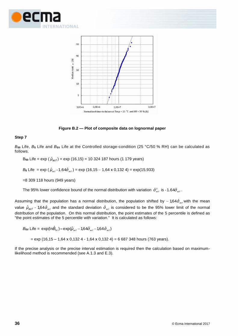
36 © Ecma International 2017
Figure B.2 — Plot of composite data on lognormal paper
Step 7
B50 Life, B5 Life and B5V Life at the Controlled storage-condition (25 °C/50 % RH) can be calculated as follows.
B50 Life = exp ( acfμ ) = exp (16,15) = 10 324 187 hours (1 179 years)
B5 Life = exp (acfacf
σμ ˆ64.1ˆ - ) = exp (16,15 1,64 х 0,132 4) = exp(15,933)
=8 309 118 hours (949 years)
The 95% lower confidence bound of the normal distribution with variation 2ˆacf
σ is -acf
σ64.1 .
Assuming that the population has a normal distribution, the population shifted by acf
σ64,1 with the mean
value acfμ - acf
σ64,1 and the standard deviation acf
σ is considered to be the 95% lower limit of the normal
distribution of the population. On this normal distribution, the point estimates of the 5 percentile is defined as "the point estimates of the 5 percentile with variation." It is calculated as follows:
B5V Life = )ˆ64,1ˆ64,1ˆexp()ˆexp(ln5 acfacfacfV
σσμB
= exp (16,15 – 1,64 х 0,132 4 - 1,64 х 0,132 4) = 6 687 348 hours (763 years).
If the precise analysis or the precise interval estimation is required then the calculation based on maximum-likelihood method is recommended (see A.1.3 and E.3).

© Ecma International 2017 37
Annex C (normative)
Disk-life estimation for Harsh storage-condition
(Arrhenius method)
C.1 Stress conditions and data-analysis steps for Arrhenius method
Here, a test method is shown for the Harsh storage-condition at higher temperature and relative humidity than that of the Controlled storage-condition (25 °C and 50 % RH).
This test method follows the scope in this document, which is based on an environment of 30 °C and 80 % RH representing the most-severe condition in which users handle and store optical disks. This test method also uses a different stress-test design that makes the use of the Arrhenius method possible.
The same assumptions and data-analysis methods apply for the ambient storage-condition, stress design, and Arrhenius equation. The Controlled storage-condition of 25 °C and 50 % RH is replaced by an expected harsher user environment of 30 °C and 80 % RH.
Table C.1 and C.2 summarize the stress design for the Arrhenius method. In case a stress condition would be destructive for the disk to be tested see Annex D.
Table C.1 — Rigorous stress-condition for use with Arrhenius method
Test
specimen
group
Test stress
condition
(incubation)
Number of
specimens
Maximum
incubation
sub-interval
time
Minimum
total
incubation
time
Intermediate
relative
humidity
Minimum
equilibration
duration time
Temp
°C
RH
% h h
RH
% h
A 85 80 20 300 1 500 30 5
B 80 80 20 400 2 000 31 7
C 75 80 20 600 3 000 32 8
D 65 80 30 800 4 000 35 10
Table C.2 — Basic stress-condition for use with Arrhenius method
Test
specimen
group
Test stress
condition
(incubation)
Number of
specimens
Maximum
incubation
sub-interval
time
Minimum
total
incubation
time
Intermediate
relative
humidity
Minimum
equilibration
duration time
Temp
°C
RH
% h h
RH
% h
A 85 80 20 250 1 000 30 5
B 75 80 20 425 1 700 32 8
C 65 80 30 600 2 400 35 10
Regarding the data-analysis steps in Annex B, Step 4 is replaced as follows.
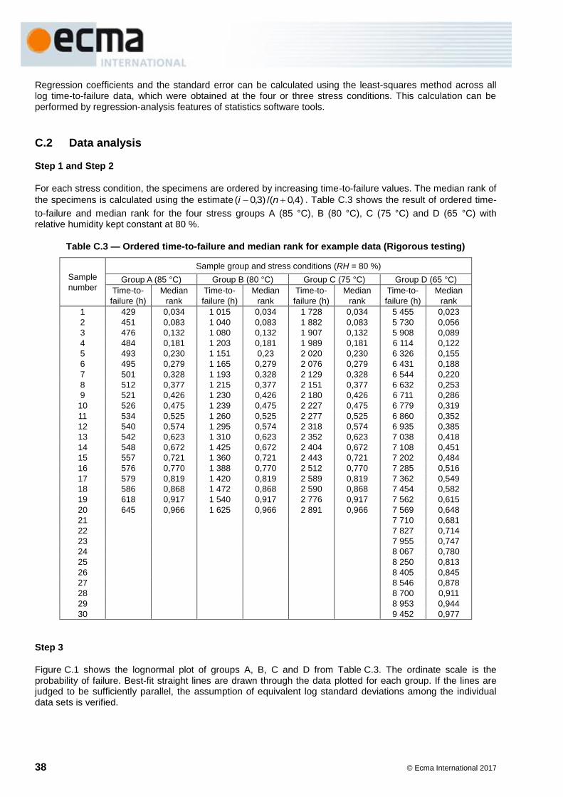
38 © Ecma International 2017
Regression coefficients and the standard error can be calculated using the least-squares method across all log time-to-failure data, which were obtained at the four or three stress conditions. This calculation can be performed by regression-analysis features of statistics software tools.
C.2 Data analysis
Step 1 and Step 2
For each stress condition, the specimens are ordered by increasing time-to-failure values. The median rank of
the specimens is calculated using the estimate )4,0/()3,0( ni . Table C.3 shows the result of ordered time-
to-failure and median rank for the four stress groups A (85 °C), B (80 °C), C (75 °C) and D (65 °C) with relative humidity kept constant at 80 %.
Table C.3 — Ordered time-to-failure and median rank for example data (Rigorous testing)
Sample
number
Sample group and stress conditions (RH = 80 %)
Group A (85 °C) Group B (80 °C) Group C (75 °C) Group D (65 °C)
Time-to-
failure (h)
Median
rank
Time-to-
failure (h)
Median
rank
Time-to-
failure (h)
Median
rank
Time-to-
failure (h)
Median
rank
1 429 0,034 1 015 0,034 1 728 0,034 5 455 0,023
2 451 0,083 1 040 0,083 1 882 0,083 5 730 0,056
3 476 0,132 1 080 0,132 1 907 0,132 5 908 0,089
4 484 0,181 1 203 0,181 1 989 0,181 6 114 0,122
5 493 0,230 1 151 0,23 2 020 0,230 6 326 0,155
6 495 0,279 1 165 0,279 2 076 0,279 6 431 0,188
7 501 0,328 1 193 0,328 2 129 0,328 6 544 0,220
8 512 0,377 1 215 0,377 2 151 0,377 6 632 0,253
9 521 0,426 1 230 0,426 2 180 0,426 6 711 0,286
10 526 0,475 1 239 0,475 2 227 0,475 6 779 0,319
11 534 0,525 1 260 0,525 2 277 0,525 6 860 0,352
12 540 0,574 1 295 0,574 2 318 0,574 6 935 0,385
13 542 0,623 1 310 0,623 2 352 0,623 7 038 0,418
14 548 0,672 1 425 0,672 2 404 0,672 7 108 0,451
15 557 0,721 1 360 0,721 2 443 0,721 7 202 0,484
16 576 0,770 1 388 0,770 2 512 0,770 7 285 0,516
17 579 0,819 1 420 0,819 2 589 0,819 7 362 0,549
18 586 0,868 1 472 0,868 2 590 0,868 7 454 0,582
19 618 0,917 1 540 0,917 2 776 0,917 7 562 0,615
20 645 0,966 1 625 0,966 2 891 0,966 7 569 0,648
21 7 710 0,681
22 7 827 0,714
23 7 955 0,747
24 8 067 0,780
25 8 250 0,813
26 8 405 0,845
27 8 546 0,878
28 8 700 0,911
29 8 953 0,944
30 9 452 0,977
Step 3
Figure C.1 shows the lognormal plot of groups A, B, C and D from Table C.3. The ordinate scale is the probability of failure. Best-fit straight lines are drawn through the data plotted for each group. If the lines are judged to be sufficiently parallel, the assumption of equivalent log standard deviations among the individual data sets is verified.
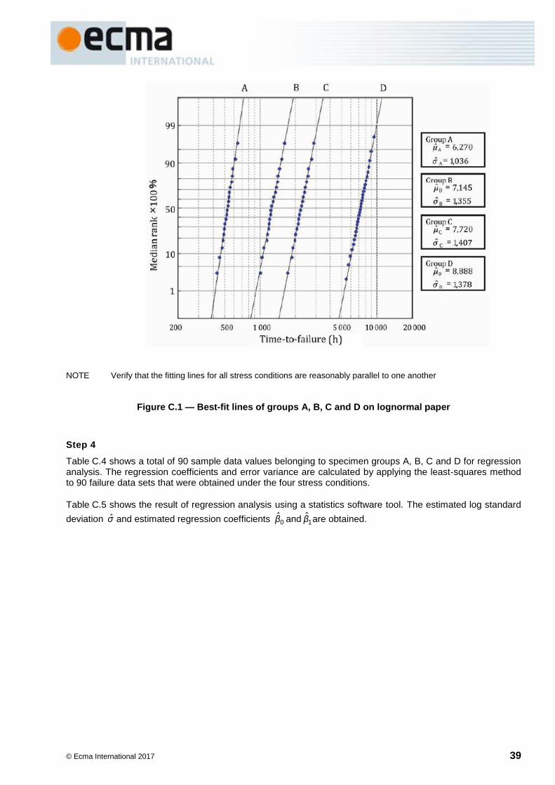
© Ecma International 2017 39
NOTE Verify that the fitting lines for all stress conditions are reasonably parallel to one another
Figure C.1 — Best-fit lines of groups A, B, C and D on lognormal paper
Step 4
Table C.4 shows a total of 90 sample data values belonging to specimen groups A, B, C and D for regression analysis. The regression coefficients and error variance are calculated by applying the least-squares method to 90 failure data sets that were obtained under the four stress conditions.
Table C.5 shows the result of regression analysis using a statistics software tool. The estimated log standard
deviation σ and estimated regression coefficients 0β and 1β are obtained.

40 © Ecma International 2017
Table C.4 — 90 sample data values for regression analysis
Number ln t x1 Number ln t x1
1 6,061 05 0,002 792
Group A
1 7,454 92 0,002 872
Group C
2 6,111 47 0,002 792 2 7,540 28 0,002 872
3 6,165 42 0,002 792 3 7,553 36 0,002 872
4 6,182 18 0,002 792 4 7,595 32 0,002 872
5 6,200 51 0,002 792 5 7,610 63 0,002 872
6 6,204 56 0,002 792 6 7,638 06 0,002 872
7 6,216 61 0,002 792 7 7,663 17 0,002 872
8 6,238 32 0,002 792 8 7,673 91 0,002 872
9 6,255 75 0,002 792 9 7,687 12 0,002 872
10 6,265 30 0,002 792 10 7,708 53 0,002 872
11 6,280 40 0,002 792 11 7,730 83 0,002 872
12 6,291 31 0,002 792 12 7,748 37 0,002 872
13 6,295 27 0,002 792 13 7,763 20 0,002 872
14 6,306 28 0,002 792 14 7,785 04 0,002 872
15 6,322 57 0,002 792 15 7,800 85 0,002 872
16 6,356 11 0,002 792 16 7,828 69 0,002 872
17 6,361 30 0,002 792 17 7,859 16 0,002 872
18 6,373 32 0,002 792 18 7,859 35 0,002 872
19 6,426 49 0,002 792 19 7,928 61 0,002 872
20 6,469 25 0,002 792 20 7,969 48 0,002 872
1 6,922 64 0,002 832
Group B
1 8,604 29 0,002 957
Group D
2 6,946 98 0,002 832 2 8,653 47 0,002 957
3 6,984 72 0,002 832 3 8,684 06 0,002 957
4 7,092 57 0,002 832 4 8,718 34 0,002 957
5 7,048 39 0,002 832 5 8,752 50 0,002 957
6 7,060 48 0,002 832 6 8,768 89 0,002 957
7 7,084 23 0,002 832 7 8,786 36 0,002 957
8 7,102 50 0,002 832 8 8,799 66 0,002 957
9 7,114 77 0,002 832 9 8,811 50 0,002 957
10 7,122 06 0,002 832 10 8,821 63 0,002 957
11 7,138 87 0,002 832 11 8,833 46 0,002 957
12 7,166 27 0,002 832 12 8,844 34 0,002 957
13 7,177 78 0,002 832 13 8,859 08 0,002 957
14 7,261 93 0,002 832 14 8,868 98 0,002 957
15 7,215 24 0,002 832 15 8,882 17 0,002 957
16 7,235 62 0,002 832 16 8,893 57 0,002 957
17 7,258 41 0,002 832 17 8,904 09 0,002 957
18 7,294 38 0,002 832 18 8,916 51 0,002 957
19 7,339 54 0,002 832 19 8,930 89 0,002 957
20 7,393 26 0,002 832 20 8,931 86 0,002 957
21 8,950 27 0,002 957
22 8,965 33 0,002 957
23 8,981 56 0,002 957
24 8,995 55 0,002 957
25 9,017 97 0,002 957
26 9,036 58 0,002 957
27 9,053 22 0,002 957
28 9,071 08 0,002 957
29 9,099 74 0,002 957
30 9,153 98 0,002 957
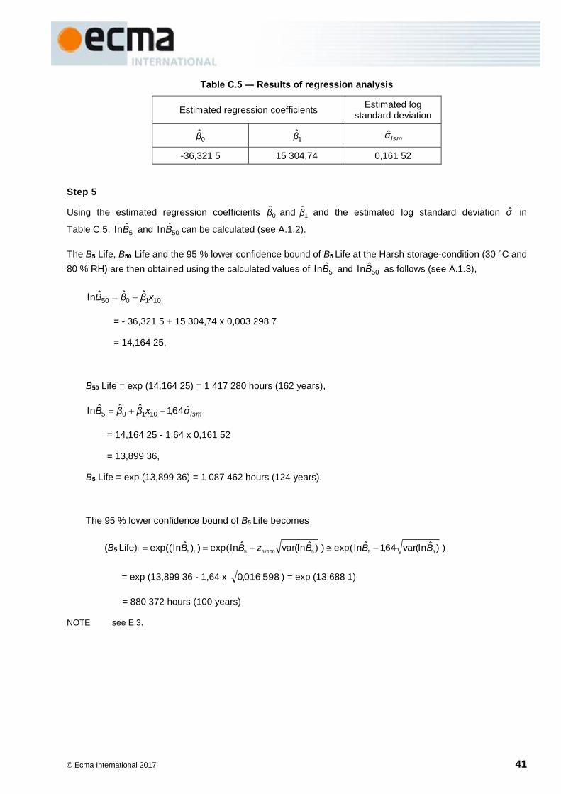
© Ecma International 2017 41
Table C.5 ― Results of regression analysis
Estimated regression coefficients Estimated log
standard deviation
0β 1β lsmσ
-36,321 5 15 304,74 0,161 52
Step 5
Using the estimated regression coefficients 0β and 1β and the estimated log standard deviation σ in
Table C.5, 5ˆlnB and 50
ˆlnB can be calculated (see A.1.2).
The B5 Life, B50 Life and the 95 % lower confidence bound of B5 Life at the Harsh storage-condition (30 °C and
80 % RH) are then obtained using the calculated values of 5ˆlnB and 50
ˆlnB as follows (see A.1.3),
101050ˆˆˆln xββB
= - 36,321 5 + 15 304,74 х 0,003 298 7
= 14,164 25,
B50 Life = exp (14,164 25) = 1 417 280 hours (162 years),
lsmσxββB ˆ64,1ˆˆˆln 10105
= 14,164 25 - 1,64 х 0,161 52
= 13,899 36,
B5 Life = exp (13,899 36) = 1 087 462 hours (124 years).
The 95 % lower confidence bound of B5 Life becomes
(B5 Life)L ))ˆvar(ln64,1ˆln(exp))ˆvar(lnˆln(exp))ˆln(exp(555100/55L5
BBBzBB
= exp (13,899 36 - 1,64 х 598016,0 ) = exp (13,688 1)
= 880 372 hours (100 years)
NOTE see E.3.

42 © Ecma International 2017

© Ecma International 2017 43
Annex D (normative)
Alternative non destructive stress-condition
In case a stress condition is destructive for the disk to be tested, an alternative stress condition shall be applied.
The stress conditions of Temp/RH used in this Ecma Standard are 85 °C/80 %, 85 °C/70 %, 85 °C/60 %, 80 °C/80 %, 75 °C/80 %, 70 °C/75 % and 65 °C/80 %.
Among these stress conditions, the most severe temperature is 85 °C. In case the stress condition with temperature 85 °C is considered to be destructive for a disk to be tested regardless of the relative humidity, it should be replaced with 80 °C in all the stress conditions with 85 °C. Recommended alternative stress-conditions for the Eyring and Arrhenius methods are shown in Table D.1, D.2, D.3 and D.4.
Table D.1 — Alternative Rigorous stress-condition for use with Eyring method
Test
specimen
group
Test stress
condition
(incubation)
Number of
specimens
Maximum
incubation
sub-interval
time
Minimum
total
incubation
time
Intermediate
relative
humidity
Minimum
equilibration
duration time
Temp
°C
RH
% h h
RH
% h
A 80 80 20 300 1 500 31 7
B 80 70 20 400 2 000 31 6
C 80 60 20 600 3 000 31 5
D 75 80 20 600 3 000 32 8
E 65 80 30 800 4 000 35 9
Table D.2 — Alternative Basic stress-condition for use with Eyring method
Test
specimen
group
Test stress
condition
(incubation)
Number of
specimens
Maximum
incubation
sub-interval
time
Minimum
total
incubation
time
Intermediate
relative
humidity
Minimum
equilibration
duration time
Temp
°C
RH
% h h
RH
% h
A 80 80 20 250 1 000 31 7
B 80 70 20 250 1 000 31 6
C 65 80 20 500 2 000 35 9
D 70 75 30 625 2 500 33 11

44 © Ecma International 2017
Table D.3 — Alternative Rigorous stress-condition for use with Arrhenius method
Test
specimen
group
Test stress
condition
(incubation)
Number of
specimens
Maximum
incubation
sub-interval
time
Minimum
total
incubation
time
Intermediate
relative
humidity
Minimum
equilibration
duration time
Temp
°C
RH
% h h
RH
% h
A 80 80 20 300 1 500 31 7
B 75 80 20 400 2 000 32 8
C 70 80 20 600 3 000 33 9
D 65 80 30 800 4 000 35 10
Table D.4 — Alternative Basic stress-condition for use with Arrhenius method
Test
specimen
group
Test stress
condition
(incubation)
Number of
specimens
Maximum
incubation
sub-interval
time
Minimum
total
incubation
time
Intermediate
relative
humidity
Minimum
equilibration
duration time
Temp
°C
RH
% h h
RH
% h
A 80 80 20 250 1 000 31 7
B 75 80 20 425 1 700 32 8
C 65 80 30 600 2 400 35 10
The amount of water absorbed by the inkjet printing label due to the stress conditions far exceeds what would be experienced in normal use and operating conditions. A disk with a label layer for inkjet printing can show a large tilt due to the excessive moisture in the label layer. Thus it is recommended to use disks without the inkjet printing label layer for the test specimen. In case to use disks with the inkjet printing label layer that shows a large tilt by the excessive moisture for the accelerated-aging test, it is recommended to set the minimum equilibration duration time long enough, as an alternative stress-condition, so that the excessive humidity goes out from that inkjet printing label layer and the large tilt disappears. To leave the disks in the test environment for a while until the large tilt disappears may also be applied.

© Ecma International 2017 45
Annex E (informative)
Interval Estimation for B5 Life using Maximum Likelihood
E.1 Lower confidence bound
Lifetime-estimation analysis (point estimation and simple interval estimation) for B5 Life and B50 Life are described in Annex A. In this Annex, a more precise analysis method for interval estimation is introduced. One may consider only the lower bound of the confidence interval to estimate lifetime.
NOTE The equations shown in this annex are for the case of complete data.
E.2 Maximum-likelihood method
To ensure that log lifetime ( y = tln ) follows the normal distribution described in A.1.2, the likelihood function
of parameters β and σ can be defined by the following equation.
J
j
n
i
ij
j
yfσβ,L
1 1
ix |)(
2
1 1
2
1exp
2
1
σ
y
σπ
ijJ
j
n
i
j βx・
where J denotes the number of specimen groups, jn denotes the number of specimens in the specimen
group j and σ is the standard deviation of the population.
The log likelihood function is then
222110
1 12
1
))((2
12ln(ln jj
J
j
n
i
ij
J
j
j xβxββyσ
nσπσβL
j
),
The maximum-likelihood estimators β and σ can be obtained by maximizing the second member of the
equation.
The estimates 210ˆandˆ,ˆ βββ are coefficients in the multiple regression equation, and the estimate σ is the
standard deviation.
The point estimation of pBln can be obtained using the estimates asσβββ ˆandˆ,ˆ,ˆ210
.ˆˆˆˆˆln 100/22110 σzxβxββB pp
Then the point estimates of 5 percentile and 50 percentile of the lifetime distribution are
σxβxββB ˆ64,1ˆˆˆˆln 20210105 and
202101050ˆˆˆˆln xβxββB
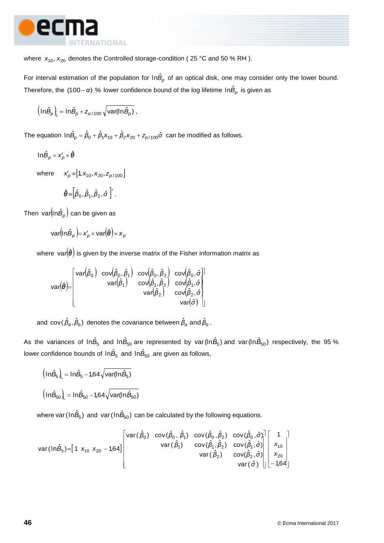
46 © Ecma International 2017
where 2010, xx denotes the Controlled storage-condition ( 25 °C and 50 % RH ).
For interval estimation of the population for pBln of an optical disk, one may consider only the lower bound.
Therefore, the %)100( α lower confidence bound of the log lifetime pBln is given as
)ˆvar(lnˆlnˆln 100/L pαpp BzBB ,
The equation σzxβxββB ˆˆˆˆˆln 100/p2021010p can be modified as follows.
θˆln pp xB
where 100/2010 ,,,1 pp zxxx
σβββ ˆ,ˆ,ˆ,ˆˆ210θ .
Then pBlnvar can be given as
ppp xxB θvarˆlnvar
where θvar is given by the inverse matrix of the Fisher information matrix as
σ
σββ
σββββ
σββββββ
ˆvar
ˆ,ˆcovˆvar
ˆ,ˆcovˆ,ˆcovˆvar
ˆ,ˆcovˆ,ˆcovˆ,ˆcovˆvar
ˆvar22
1211
020100
θ
and )ˆ,ˆ(cov ba ββ denotes the covariance between ba ββ ˆandˆ .
As the variances of 5ˆlnB and 50
ˆlnB are represented by )ˆ(lnvar 5Β and )ˆ(lnvar 50Β respectively, the 95 %
lower confidence bounds of 5ˆlnB and 50
ˆlnB are given as follows,
)ˆvar(ln64,1ˆlnˆln 55L5 BBB
)ˆvar(ln64,1ˆlnˆln 5050L50 BBB
where )ˆln(var 5Β and )ˆln(var 50Β can be calculated by the following equations.
64,1
1
)ˆ(var
)ˆ,ˆcov()ˆ(var
)ˆ,ˆ(cov)ˆ,ˆ(cov)ˆ(var
)ˆ,ˆ(cov)ˆ,ˆ(cov)ˆ,ˆ(cov)ˆ(var
64,11)ˆln(var20
10
22
1211
020100
20105x
x
σ
σββ
σββββ
σββββββ
xxB
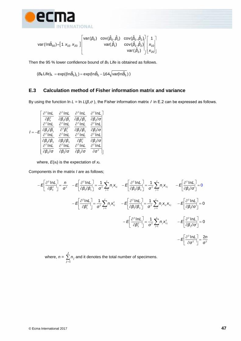
© Ecma International 2017 47
20
10
2
211
20100
201050
1
)ˆ(var
)ˆ,ˆ(cov)ˆvar(
)ˆ,ˆ(cov)ˆ,ˆ(cov)(var
1)ˆln(var
x
x
β
βββ
βββββ
xxB
Then the 95 % lower confidence bound of B5 Life is obtained as follows.
(B5 Life)L )ˆvar(ln64,1ˆ(lnexp))ˆ(lnexp( 55L5 BBB )
E.3 Calculation method of Fisher information matrix and variance
By using the function ln L = ln L(β,σ ), the Fisher information matrix I in E.2 can be expressed as follows.
2
2
2
2
1
2
0
22
2
2
2
2
21
2
20
21
2
21
2
2
1
2
2
10
20
2
20
2
10
2
2
0
2
lnlnlnln
lnlnlnln
lnlnlnln
lnlnlnln
σ
L
σβ
L
σβ
L
σβ
L
σβ
L
β
L
ββ
L
ββ
L
σβ
L
ββ
L
β
L
ββ
L
σβ
L
ββ
L
ββ
L
β
L
EI
where, E(xi) is the expectation of xi.
Components in the matrix I are as follows;
22
0
2 ln
σ
n
β
LE
J
j
jjxn
σββ
LE
1
12
10
2 1ln
J
j
jjxn
σββ
LE
1
22
20
2 1ln
σβ
LE
0
2 ln0
2
1
1
22
1
2 1lnj
J
j
jxn
σβ
LE
jj
J
j
jxxn
σββ
LE
21
1
2
21
2 1ln
0
ln
1
2
σβ
LE
2
2
1
22
2
2 1lnj
J
j
jxn
σβ
LE
0
ln
2
2
σβ
LE
22
2 2ln
σ
n
σ
LE
where, n =
J
jjn
1
and it denotes the total number of specimens.
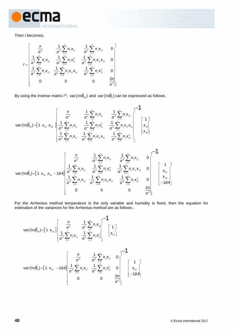
48 © Ecma International 2017
Then I becomes,
2
2
2
1
221
1
2
1
22
21
1
2
2
1
1
2
1
12
1
22
1
122
2000
0111
0111
011
σ
n
xnσ
xxnσ
xnσ
xxnσ
xnσ
xnσ
xnσ
xnσσ
n
I
j
J
j
jjj
J
j
j
J
j
jj
jj
J
j
jj
J
j
j
J
j
jj
J
j
jj
J
j
jj
By using the inverse matrix I-1, )ˆln(var50
B and )ˆln(var5
B can be expressed as follows.
20
10
2
2
1
221
1
2
1
22
21
1
2
2
1
1
2
1
12
1
22
1
122
201050
1
111
111
11
1)ˆln(var
1
x
x
xnσ
xxnσ
xnσ
xxnσ
xnσ
xnσ
xnσ
xnσσ
n
xxB
j
J
j
jjj
J
j
j
J
j
jj
jj
J
j
jj
J
j
j
J
j
jj
J
j
jj
J
j
jj
64,1
1
2000
0111
0111
011
64,11)ˆln(var20
10
2
2
2
1
221
1
2
1
22
21
1
2
2
1
1
2
1
12
1
22
1
122
20105
1
x
x
σ
n
xnσ
xxnσ
xnσ
xxnσ
xnσ
xnσ
xnσ
xnσσ
n
xxB
j
J
j
jjj
J
j
j
J
j
jj
jj
J
j
jj
J
j
j
J
j
jj
J
j
jj
J
j
jj
For the Arrhenius method temperature is the only variable and humidity is fixed, then the equation for estimation of the variances for the Arrhenius method are as follows:.
102
1
1
2
1
12
1
122
1050
1
11
1
1)ˆln(var
1
xxn
σxn
σ
xnσσ
n
xB
j
J
j
j
J
j
jj
J
j
jj
64,1
1
200
011
01
64,11)ˆln(var10
2
2
1
1
2
1
12
1
122
105
1
x
σ
n
xnσ
xnσ
xnσσ
n
xBj
J
j
j
J
j
jj
J
j
jj
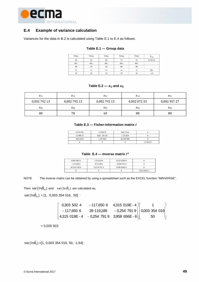
© Ecma International 2017 49
E.4 Example of variance calculation
Variances for the data in B.2 is calculated using Table E.1 to E.4 as follows:
Table E.1 — Group data
Table E.2 — x1j and x2j
Table E.3 — Fisher-information matrix I
Table E.4 — Inverse matrix I-1
NOTE The inverse matrix can be obtained by using a spreadsheet such as the EXCEL function "MINVERSE".
Then )ˆln(var50
B and )ˆln(var 5B are calculated as,
)ˆln(var50
B = [1, 0,003 354 016, 50] ·
50
016354003,0
1
6-E656958,39791254,04-E019315,4
9791254,0189,119396650,117
4-E019315,46650,1174502303,0
= 0,020 915
)ˆln(var5
B =[1, 0,003 354 016, 50, -1,64] ·

50 © Ecma International 2017
64,1
50
016354003,0
1
5-E056962,7000
06-E656958,39791254,04-E019315,4
09791254,0189,119396650,117
04-E019315,46650,1174502303,0
= 0,021 129.
NOTE The matrix multiplication can be calculated using a spreadsheet such as the EXCEL function "MMULT".
© Ecma International 2017 51
Annex F (informative)
RSER measurement of BD disks
The Max RSER value of 10-3 was adopted as suitable for evaluating the time-to-failure in accelerated stress testing of BD disks. The ECC used for BD is powerful enough and has better error-correction capability than that of DVD at RSER = 10-3.[8][9]
RSER excludes burst errors of length ≥ 40 bytes. But it is still affected by bursts shorter than 40 bytes.
When measuring disks, manual handling of disks is inevitable. In order to avoid introducing short bursts, it is important to take care not to leave fingerprints on the surface of disks, especially before recording initial data.
If the RSER should increase unexpectedly (especially near the outer edge of disk), it is recommended to wipe off any fingerprints and re-measure the RSER.

52 © Ecma International 2017
© Ecma International 2017 53
Bibliography
[1] ISO/IEC 10149, Information technology — Data interchange on read-only 120 mm optical data disks (CD-ROM)
[2] ISO/IEC 16448, Information technology — 120 mm DVD — Read-only disk
[3] ISO/IEC 16449, Information technology — 80 mm DVD — Read-only disk
[4] ISO 18927, Imaging materials — Recordable compact disc systems — Method for estimating the life expectancy based on the effects of temperature and relative humidity
[5] Experimental statistics, US National Bureau of Standards Handbook 91, 1963
[6] Applied Regression Analysis, Draper and Smith, Wiley Edition 2
[7] Statistical Methods for Reliability Data, Meeker, Escobar, 1998, John Wiley & Sons Inc.
[8] V. Bagdonavičius and M. Nikulin, Accelerated Life Models: Modeling and statistical analysis, Chapman & Hall/CRC, 2002
[9] J. F. Lawless, Statistical Models and Methods for Lifetime Data, 2nd Ed., Wiley, 2003
[10] W. Yamamoto, C. Kumazaki, and K. Suzuki, On Estimation of Archival Lifetime Distribution of Writable Optical Discs, Proceeding of the 21st Symposium on Phase Change Optical Information Storage PCOS 2009, pp.72-75, 2009
[11] White Paper Blu-ray Disc™ Format BD-ROM 9th Ed., August, 2015. Available from http://www.blu-raydisc.com/Assets/Downloadablefile/White%20Paper%20BD-ROM_Part1_9th_20150806_clean.pdfWhite Paper Blu-ray Disc™ Format BD-ROM 8th December,
[12] White Paper Blu-ray Disc™ Format General 4th Ed., August, 2015. Available from http://www.blu-raydisc.com/Assets/Downloadablefile/White_Paper_General_4th_20150817_clean.pdf

© Ecma International 2017


![[MS-WPE376]: WordPad ECMA 376 Standards Support · WordPad ECMA 376 Standards Support](https://static.documents.pub/doc/80x56/5fab533dea0e1c27ad282e55/ms-wpe376-wordpad-ecma-376-standards-support-wordpad-ecma-376-standards-support.jpg)


