Final projectCEE 744 Advanced Structural Dynamics

Dynamic Analysis of the Elizabeth Ashman Bridge

University of Wisconsin, MadisonSpring 2013

Nasser M. Abbasi

May 16, 2014

Contents

1 Introduction 5

2 step one. Displacements at joints S15L, S07L and 21 52.1 Results . . . . . . . . . . . . . . . . . . . . . . . . . . . . . . . . . . . . . . . . . . 52.2 Method used . . . . . . . . . . . . . . . . . . . . . . . . . . . . . . . . . . . . . . . 5

3 Step two, period and damping calculations 123.1 Results . . . . . . . . . . . . . . . . . . . . . . . . . . . . . . . . . . . . . . . . . . 123.2 Method used . . . . . . . . . . . . . . . . . . . . . . . . . . . . . . . . . . . . . . . 12

4 Step three. Modal analysis 144.1 Results . . . . . . . . . . . . . . . . . . . . . . . . . . . . . . . . . . . . . . . . . . 14

5 Step four. Solving for response under simulated marching band 205.1 Results . . . . . . . . . . . . . . . . . . . . . . . . . . . . . . . . . . . . . . . . . . 205.2 Method . . . . . . . . . . . . . . . . . . . . . . . . . . . . . . . . . . . . . . . . . . 23

6 Step five. Stress results 316.1 Results . . . . . . . . . . . . . . . . . . . . . . . . . . . . . . . . . . . . . . . . . . 31

6.1.1 additional results . . . . . . . . . . . . . . . . . . . . . . . . . . . . . . . . . 316.2 Method . . . . . . . . . . . . . . . . . . . . . . . . . . . . . . . . . . . . . . . . . . 34

7 Appendix 367.1 SAP2000 definitions used in this report . . . . . . . . . . . . . . . . . . . . . . . . . 36

7.1.1 Local axis signs . . . . . . . . . . . . . . . . . . . . . . . . . . . . . . . . . 367.1.2 Frame element internal forces output convention . . . . . . . . . . . . . . . . 377.1.3 SAP2000 S11 description (stress calculations) . . . . . . . . . . . . . . . . . 387.1.4 SAP2000 shell element internal forces/stresses output convention . . . . . . . 39

7.2 references . . . . . . . . . . . . . . . . . . . . . . . . . . . . . . . . . . . . . . . . . 39

1

List of Figures1 Adding missing joints to bridge database . . . . . . . . . . . . . . . . . . . . . . . . 62 connected ramp to bridge using RBEAMS . . . . . . . . . . . . . . . . . . . . . . . 73 adding vertical load pattern for step one use . . . . . . . . . . . . . . . . . . . . . . . 84 adding vertical load to joint S15L . . . . . . . . . . . . . . . . . . . . . . . . . . . . 95 adding vertical load pattern for step one use . . . . . . . . . . . . . . . . . . . . . . . 106 adding vertical load to joint 21 . . . . . . . . . . . . . . . . . . . . . . . . . . . . . . 107 vertical acceleration time records . . . . . . . . . . . . . . . . . . . . . . . . . . . . 128 zoomed view on the vertical acceleration time records . . . . . . . . . . . . . . . . . 139 3D axis orientation used . . . . . . . . . . . . . . . . . . . . . . . . . . . . . . . . . 1410 Stress at base of column, mode 1 . . . . . . . . . . . . . . . . . . . . . . . . . . . . . 1611 Stress at base of column, mode 2 . . . . . . . . . . . . . . . . . . . . . . . . . . . . . 1612 Stress at base of column, mode 3 . . . . . . . . . . . . . . . . . . . . . . . . . . . . . 1713 Stress at base of column, mode 4 . . . . . . . . . . . . . . . . . . . . . . . . . . . . . 1714 Stress at base of column, mode 5 . . . . . . . . . . . . . . . . . . . . . . . . . . . . . 1815 Stress at base of column, mode 6 . . . . . . . . . . . . . . . . . . . . . . . . . . . . . 1816 Stress at base of column, mode 7 . . . . . . . . . . . . . . . . . . . . . . . . . . . . . 1917 Stress at base of column, mode 8 . . . . . . . . . . . . . . . . . . . . . . . . . . . . . 1918 node locations for cantilever beams . . . . . . . . . . . . . . . . . . . . . . . . . . . 2019 relative displacements of joints on ramp . . . . . . . . . . . . . . . . . . . . . . . . . 2120 Displacement of node 20 on ramp column 3 during dynamic response . . . . . . . . . 2221 Axial load P variation in column during during dynamic excitation . . . . . . . . . . 2222 movie of first 20 seconds during marching band motion . . . . . . . . . . . . . . . . 2323 Description of step 4, solving for response under dynamic marching band . . . . . . . 2424 Relation between load pattern and load case . . . . . . . . . . . . . . . . . . . . . . . 2525 Defining live load pattern LL . . . . . . . . . . . . . . . . . . . . . . . . . . . . . . . 2526 Adding live load to bridge floors . . . . . . . . . . . . . . . . . . . . . . . . . . . . . 2627 Adding LL load to ramp RBEAMs . . . . . . . . . . . . . . . . . . . . . . . . . . . 2628 Adding 10 kips load on right side of RAMP . . . . . . . . . . . . . . . . . . . . . . . 2729 Adding time history function . . . . . . . . . . . . . . . . . . . . . . . . . . . . . . . 2730 Adding MODAL load case . . . . . . . . . . . . . . . . . . . . . . . . . . . . . . . . 2831 defining marching band dynamic load case . . . . . . . . . . . . . . . . . . . . . . . 2832 defining combination load case . . . . . . . . . . . . . . . . . . . . . . . . . . . . . 2933 modified section property RBEAM . . . . . . . . . . . . . . . . . . . . . . . . . . . 2934 Plot of stress vs. time during dynamic loading . . . . . . . . . . . . . . . . . . . . . . 3135 max/min of S11 stress at base of column, Marching band case . . . . . . . . . . . . . 3236 Max/min of axial load at base of column, Marching band case . . . . . . . . . . . . . 3237 Max/min M22 at base of column, Marching band case . . . . . . . . . . . . . . . . . . 3338 Max/min M33 at base of column, Marching band case . . . . . . . . . . . . . . . . . . 3339 Stress S11 at base of column, Combination test case . . . . . . . . . . . . . . . . . . 3340 Axial load at base of column, Combination test case . . . . . . . . . . . . . . . . . . 3441 Max/min M22 at base of column, Combination test case . . . . . . . . . . . . . . . . . 3442 Max/min M33 at base of column, Combination test case . . . . . . . . . . . . . . . . . 3443 SAP2000 local axis signs . . . . . . . . . . . . . . . . . . . . . . . . . . . . . . . . . 3644 SAP2000 Frame element internal forces output convention . . . . . . . . . . . . . . . 37

2

45 SAP2000 S11 description . . . . . . . . . . . . . . . . . . . . . . . . . . . . . . . . 3846 SAP2000 shell element internal forces/stresses output convention . . . . . . . . . . . 39

3

List of Tables1 Displacements at joint 21 . . . . . . . . . . . . . . . . . . . . . . . . . . . . . . . . . 52 Period and damping . . . . . . . . . . . . . . . . . . . . . . . . . . . . . . . . . . . 123 Description of each mode . . . . . . . . . . . . . . . . . . . . . . . . . . . . . . . . 154 Stress calculation result for step 5 . . . . . . . . . . . . . . . . . . . . . . . . . . . . 31

4

1 IntroductionResults of each step are given in separate section. Each section has two parts, the first shows the resultsand the second describes the methods and analysis performed to obtain the results.

2 step one. Displacements at joints S15L, S07L and 21

2.1 Results

Joint U1 U2 U3 R1 R2 R3ft ft ft rad rad rad

S07L 0.000179 -0.003174 0.021538 -0.000119 0.000098 4.253E-06S15L 0.000035 -0.003104 -0.032437 -0.000216 -0.001357 0.000029

Joint U1 U2 U3 R1 R2 R3ft ft ft rad rad rad

21 0.007568 -0.002749 -0.024066 -0.000011 0.001533 -0.000120

Table 1: Displacements at joint 21

2.2 Method usedProblem description is

Find the deflections of the arch portion of the bridge at node or jointS15L and S07L when a 10k downward point load is applied at joint S15L.Also find the displacements of joint 21 on the ramp when a 10k downwardload is applied at that joint.

There are the steps performed

1. The original bridge database was not complete. The missing joints were first added. Afteropening the database, the XZ view was selected. This is needed as it was found it is not possibleto add a point in the default 3D view.

2. Clicked on the Draw Special joint icon located on the left edge of the window. This is thesmall blue square in version 15 of SAP2000.

3. Clicked on an empty area on the screen to add a point.

4. Right clicked on the added point again to bring up a pop-up menu dialogue that was used fordata entry of given coordinates.

5. Filled the coordinates and the labels as given in the PDF file.

5

6. Made sure that the menu item in the JOINT COORDINATES called SPECIAL Jt (User Def) islabeled YES. If this is labeled NO then this procedure did not work and the point was not added.

7. Clicked UPDATE DISPLAY then clicked OK.

8. Verified that the points were added by selecting DISPLAY->SHOW TABLES then using the pop-upmenu and searched Joint Coordinates

9. Figure 1 shows part of the joints coordinates table after completing the above steps.

Figure 1: Adding missing joints to bridge database

Partial listing of joints is shown below

SAP2000 v15.0.1 5/2/13 22:18:29Table: Joint Coordinates

Joint CoordSys CoordType XorR Y Z SpecialJt GlobalX GlobalY GlobalZft ft ft ft ft ft

1 GLOBAL Cartesian -4.1200 122.2500 74.0750 No -4.1200 122.2500 74.07502 GLOBAL Cartesian 4.1200 122.2500 74.0750 No 4.1200 122.2500 74.07503 GLOBAL Cartesian -7.9700 152.5000 58.2900 No -7.9700 152.5000 58.29004 GLOBAL Cartesian 7.9500 152.5000 58.2900 No 7.9500 152.5000 58.29005 GLOBAL Cartesian 0.0000 175.8000 36.1100 Yes 0.0000 175.8000 36.11006 GLOBAL Cartesian 0.0000 175.8000 53.3800 Yes 0.0000 175.8000 53.38007 GLOBAL Cartesian 6.0000 175.0000 53.3800 Yes 6.0000 175.0000 53.38008 GLOBAL Cartesian -6.0000 175.0000 53.3800 Yes -6.0000 175.0000 53.38009 GLOBAL Cartesian 3.5600 157.8000 54.5400 No 3.5600 157.8000 54.5400

10 GLOBAL Cartesian -3.5600 157.8000 54.5400 No -3.5600 157.8000 54.540011 GLOBAL Cartesian 0.0000 219.2000 50.7300 Yes 0.0000 219.2000 50.730012 GLOBAL Cartesian 0.0000 219.2000 39.3100 Yes 0.0000 219.2000 39.310013 GLOBAL Cartesian 0.0000 219.2000 32.7400 Yes 0.0000 219.2000 32.740014 GLOBAL Cartesian 12.0000 217.6000 50.7300 Yes 12.0000 217.6000 50.730015 GLOBAL Cartesian -12.0000 217.6000 39.3100 Yes -12.0000 217.6000 39.310016 GLOBAL Cartesian -7.0000 179.7600 36.7400 Yes -7.0000 179.7600 36.740017 GLOBAL Cartesian 0.0000 265.5700 29.8700 Yes 0.0000 265.5700 29.870018 GLOBAL Cartesian 0.0000 265.5700 42.5100 Yes 0.0000 265.5700 42.510019 GLOBAL Cartesian 0.0000 265.5700 44.8600 Yes 0.0000 265.5700 44.860020 GLOBAL Cartesian 0.0000 265.5700 47.0300 Yes 0.0000 265.5700 47.030021 GLOBAL Cartesian 18.0000 263.1700 47.0300 Yes 18.0000 263.1700 47.030022 GLOBAL Cartesian -18.0000 263.2000 42.5100 Yes -18.0000 263.2000 42.510023 GLOBAL Cartesian 0.0000 283.5700 44.8600 Yes 0.0000 283.5700 44.8600

6

10. Connected the joints added above to the bridge in order to establish the ramp. Figure 2 is screenshot showing the ramp connected to bridge. RBEAM elements are used.

Figure 2: connected ramp to bridge using RBEAMS

11. Before adding the 10 kips downwards load, a load pattern is defined. Selected DEFINE->LOAD PATTERNSand added new load pattern called S15L of type DEAD with self weight multiplier 0.

12. 10 kips downwards load at joint S15L was added. This was done by clicking on the joint andright clicking again. Using the pop up menu that appeared the value minus 10 was entered.Minus sign was used since load is downwards. The load pattern selected was S15L. Figure 3shows the result.

7

Figure 3: adding vertical load pattern for step one use

13. Clicked on RUN ANALYSIS. In the set load case to run case S15L was the only one se-lected. All other load cases, including DEAD was not selected. This was done to obtain re-sult due to vertical load only. Model was locked now. After run was completed, clicked onDISPLAY->SHOW TABLES->JOINT DISPACEMENTS and located nodes S15L and S07L to findthe node displacements. Figure 4 shows the result of this step

8

Figure 4: adding vertical load to joint S15L

In addition a listing from the table is shown below

SAP2000 v15.0.1 5/3/13 1:35:52Table: Joint DisplacementsJoint OutputCase CaseType U1 U2 U3 R1 R2 R3

ft ft ft Radians Radians Radians

S07L S15L LinStatic 0.000179 -0.003174 0.021538 -0.000119 0.000098 4.253E-06S15L S15L LinStatic 0.000035 -0.003104 -0.032437 -0.000216 -0.001357 0.000029

14. Before adding the 10 kips downwards load to node 21, a load pattern is defined for use. SelectedDEFINE->LOAD PATTERNS and added new load pattern called node21 of type DEAD with selfweight multiplier 0.

15. 10 kips downwards load at joint 21 was now added. This was done by clicking on the jointand right clicking aging. Using the pop-up menu that appeared the value minus 20 was entered.Minus sign was used since load is downwards. The load pattern selected was node20. Figure 5shows this step.

9

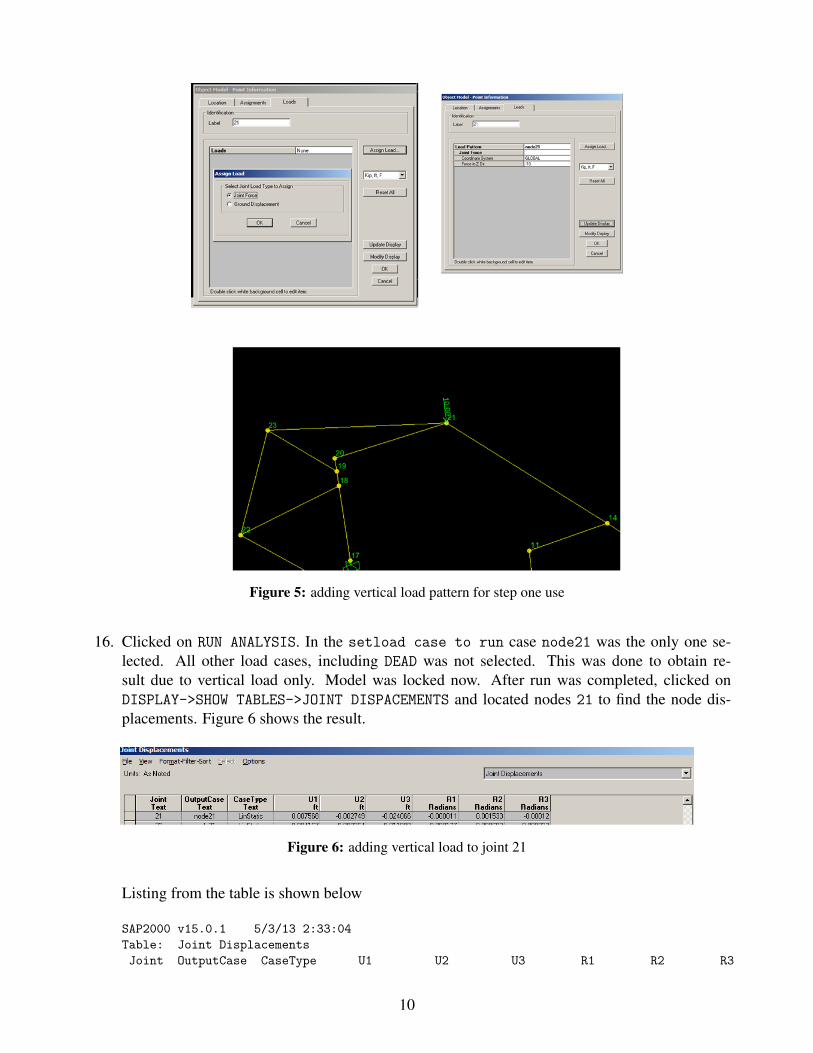
Figure 5: adding vertical load pattern for step one use

16. Clicked on RUN ANALYSIS. In the setload case to run case node21 was the only one se-lected. All other load cases, including DEAD was not selected. This was done to obtain re-sult due to vertical load only. Model was locked now. After run was completed, clicked onDISPLAY->SHOW TABLES->JOINT DISPACEMENTS and located nodes 21 to find the node dis-placements. Figure 6 shows the result.

Figure 6: adding vertical load to joint 21

Listing from the table is shown below

SAP2000 v15.0.1 5/3/13 2:33:04Table: Joint DisplacementsJoint OutputCase CaseType U1 U2 U3 R1 R2 R3

10

ft ft ft Radians Radians Radians

21 node21 LinStatic 0.007568 -0.002749 -0.024066 -0.000011 0.001533 -0.000120

11

3 Step two, period and damping calculations

3.1 ResultsThe result is shown in table 2

Natural period T (sec) Natural frequency fn (hz) critical damping ratio ζ

0.5 2.0 0.0014%

Table 2: Period and damping

3.2 Method usedThis is the problem description

Two people jogging across the bridge created the vertical acceleration recordsshown below. Each set of pulses is when the joggers were running, in betweenthey stopped. Once they stopped it is as if the bridge had an initial displacementand velocity and then decayed in free vibration. Using the enlarged portionof the record estimate - the natural period of the structure and the % damping.

Figure 7: vertical acceleration time records

The above profile can be used as free the vibration profile. The method of logarithmic decrement wasused to obtain the natural period and ζ (damping critical coefficient). Figure 8 shows a closer zoomview of the above plot in order to estimate the period. It shows the natural period to be around 10division.

12

Figure 8: zoomed view on the vertical acceleration time records

The units used are sec*20, therefore natural period is T = 1020 = 0.5 sec. Hence natural frequency

is f = 2 hz.To obtain the damping ζ , a number of methods can be used. The more accurate methods uses more

peaks. Using N = 35 as number of peaks and using method of series expansion ζ can be found. Fromthe above plot the value of first peak is 55940 and value of peak number 35 was found to be 55770.Hence

y0

y0 +N= 1+2πNζ

ζ =1

35(2π)

55940−5577055770

= 1.3861×10−5

= 0.0014%

13

4 Step three. Modal analysis

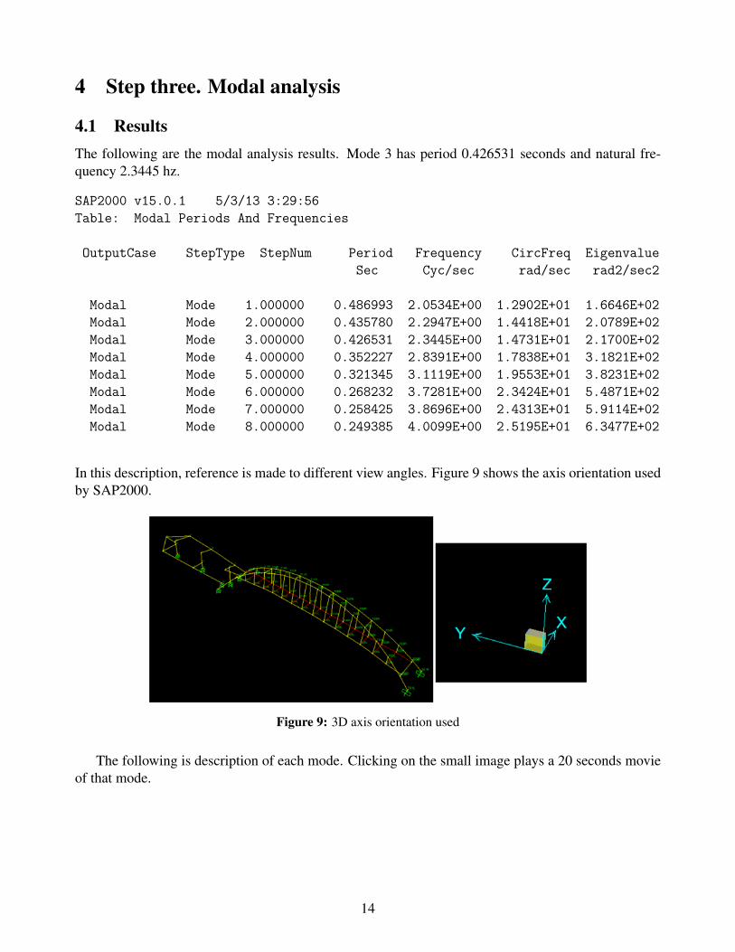
4.1 ResultsThe following are the modal analysis results. Mode 3 has period 0.426531 seconds and natural fre-quency 2.3445 hz.

SAP2000 v15.0.1 5/3/13 3:29:56Table: Modal Periods And Frequencies

OutputCase StepType StepNum Period Frequency CircFreq EigenvalueSec Cyc/sec rad/sec rad2/sec2

Modal Mode 1.000000 0.486993 2.0534E+00 1.2902E+01 1.6646E+02Modal Mode 2.000000 0.435780 2.2947E+00 1.4418E+01 2.0789E+02Modal Mode 3.000000 0.426531 2.3445E+00 1.4731E+01 2.1700E+02Modal Mode 4.000000 0.352227 2.8391E+00 1.7838E+01 3.1821E+02Modal Mode 5.000000 0.321345 3.1119E+00 1.9553E+01 3.8231E+02Modal Mode 6.000000 0.268232 3.7281E+00 2.3424E+01 5.4871E+02Modal Mode 7.000000 0.258425 3.8696E+00 2.4313E+01 5.9114E+02Modal Mode 8.000000 0.249385 4.0099E+00 2.5195E+01 6.3477E+02

In this description, reference is made to different view angles. Figure 9 shows the axis orientation usedby SAP2000.

Figure 9: 3D axis orientation used

The following is description of each mode. Clicking on the small image plays a 20 seconds movieof that mode.

14

mode 1 Bridge main body vibrates sinusoidally in the YZ plan with almost a full sin wave beingdescribed along the full length of the bridge. Ramp shows little vibration. Little motion inX direction. ashdynstat_mode_1.swf

mode 2 Similar to mode 1 but with larger amplitudes. Bridge vibration remained in the YZ plan.Ramp remains with little motionashdynstat_mode_2.swf

mode 3 This is the ramp torsion mode. Ramp shows large twisting motion around the Y axis. Mainbridge body now vibrates sideways moving in the X axes direction. The top of the bridgeis tilting sidways more than the floor. ashdynstat_mode_3.swf

mode 4 Larger twists on the main bridge. Twist is around the Z axis where one half of the bridgeswings to one side and the other half to the opposite side. Ramp has less torsion comparedto mode 3. ashdynstat_mode_4.swf

mode 5 Both ramp and bridge now show large vibration. On the bridge, more twisting vibration areseen around the Z axis going through the middle of the bridge. Little vibration in the XYplan (up and down). Most of vibration is sideways. The half of the bridge connected to theramp is vibrating in opposite direction to the ramp (out of phase with ramp). ashdynstat_mode_5.swf

mode 6 On the bridge, larger torsion vibration around the Z axis in the middle of the bridge. Rampappears to vibrate less than in mode 5. ashdynstat_mode_6.swf

mode 7 Bridge floor vibration now in the YZ plane (vertically up and down) with larger verticalamplitude in the middle of the bridge. Almost two full sin wave can be seen across the fullspan of the bridge. Ramp appears to vibrate much less than it did in mode 7. ashdynstat_mode_7.swf

mode 8 Bridge has large torsional motion around the Y axis (Axis along its length). Bridge almostcloses on itself near the top. The part of the Ramp attached to the bridge moves in phasewith the bridge motion. ashdynstat_mode_8.swf

Table 3: Description of each mode

The maximum stress at the base of the column (label 11) in the ramp was also found for each mode.This was done using SAP2000 v15.1 which has this added feature. The following diagrams give stressS11 for each mode.

15

Figure 10: Stress at base of column, mode 1

Figure 11: Stress at base of column, mode 2

16

Figure 12: Stress at base of column, mode 3

Figure 13: Stress at base of column, mode 4

17

Figure 14: Stress at base of column, mode 5

Figure 15: Stress at base of column, mode 6

18

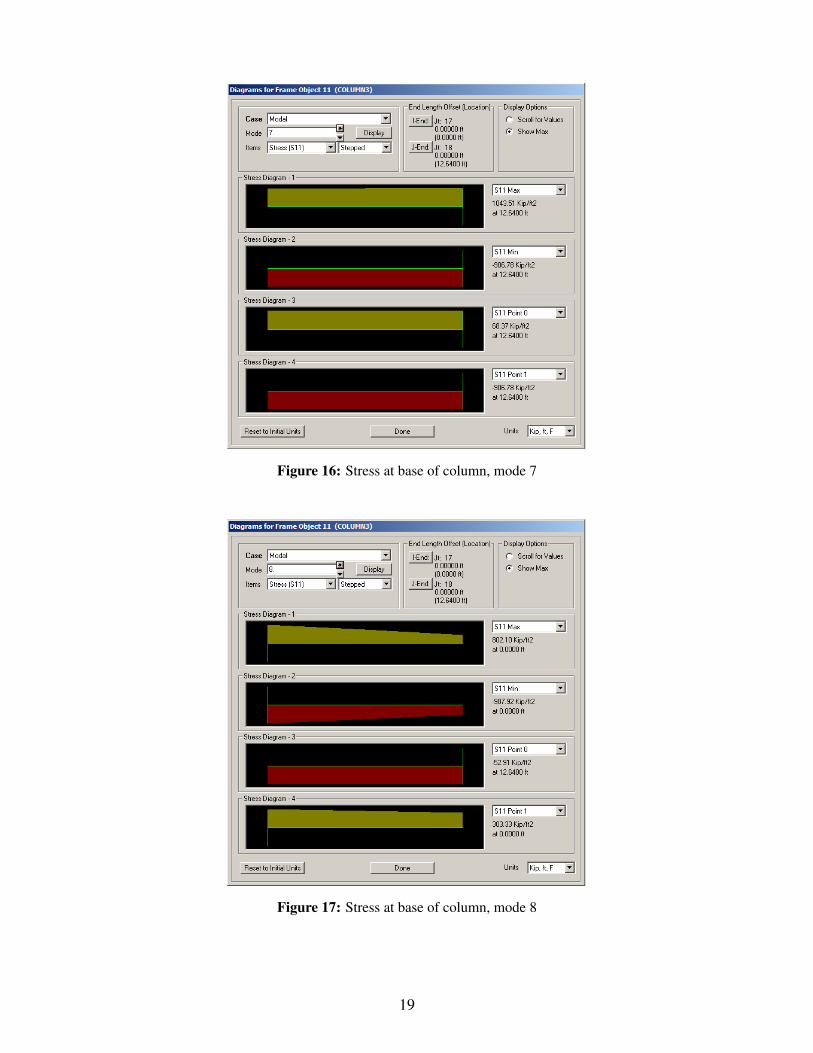
Figure 16: Stress at base of column, mode 7

Figure 17: Stress at base of column, mode 8

19

5 Step four. Solving for response under simulated marching band

5.1 ResultsThe nodes to find the displacements for are marked and given in figure ??.

Figure 18: node locations for cantilever beams

The result is shown below. The labels for local axes for joints are shown below, and are the sameas the global axes. This is from SAP2000 help section

By default, the joint local 1-2-3 coordinate system is identical tothe global X-Y-Z coordinate system

Therefore, U1 is in the X direction, and U2 in the Y direction, and U3 is the vertical displacement.

SAP2000 v15.0.1 5/4/13 1:02:04Table: Joint DisplacementsJoint OutputCase StepType U1 U2 U3 R1 R2 R3

ft ft ft Radians Radians Radians20 COMO Max 0.146711 0.019285 -0.000479 0.001667 0.015544 0.00054220 COMO Min -0.141382 -0.017992 -0.000676 -0.001788 -0.013209 -0.000675

21 COMO Max 0.144476 0.034315 0.262294 0.002986 0.022603 0.00101721 COMO Min -0.139764 -0.037636 -0.375865 0.000383 -0.015478 -0.001261

22 COMO Max 0.082805 0.009682 0.236030 0.003108 0.014103 -0.00001222 COMO Min -0.083333 -0.005028 -0.305074 -0.000501 -0.018799 -0.000326

23 COMO Max 0.123308 0.015499 0.013802 0.001111 0.015690 0.00058323 COMO Min -0.123593 -0.014890 -0.049072 -0.002825 -0.014603 -0.000494

20

Figure 19 shows screen shot of the deformed part of the ramp with the above joints marked on thediagram showing the relative displacement for better illustration.

Figure 19: relative displacements of joints on ramp

The following text file contains the result for all nodes. step_4_beam_result.txtIn addition, below are plots of nodal displacements of node 20, on top of column labeled 11 on the

ramp (this is the column being analyzed for stress). This plot shows that it took about 20 seconds fordynamic loading to settle down.

This means after 20 second of the marching band moving into the ramp, the ramp vibration reachedsteady state, therefore, the ramp is now vibrating at the same forcing frequency and transient responseof the ramp has completed.

21

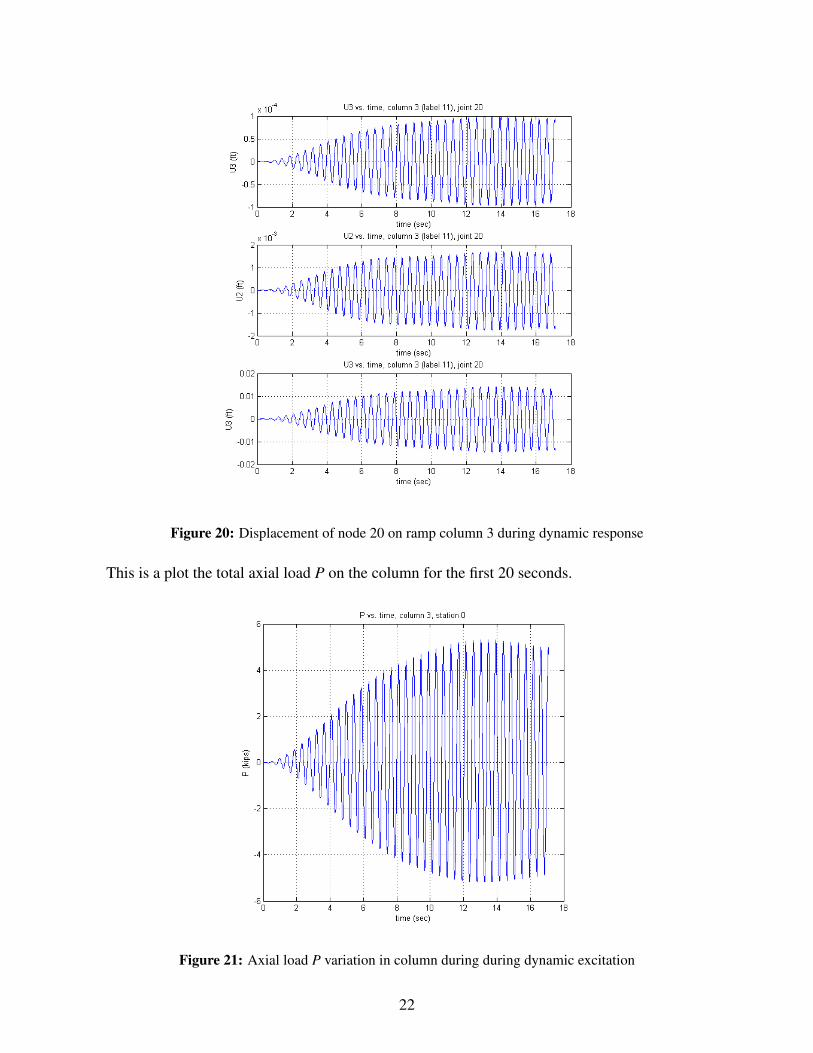
Figure 20: Displacement of node 20 on ramp column 3 during dynamic response

This is a plot the total axial load P on the column for the first 20 seconds.

Figure 21: Axial load P variation in column during during dynamic excitation

22

This is movie of the first 20 seconds of the bridge vibration during marching band motion.

Figure 22: movie of first 20 seconds during marching band motion

Node displacement for joint 20 under marching band (time history) is given below. The output isin this file node_20_final_displacement.txt

This is partial listing of the table from SAP2000.SAP2000 v15.0.1 5/3/13 5:24:47Table: Joint Displacements

Joint OutputCase CaseType StepType StepNum U1 U2 U3 R1 R2 R3ft ft ft Radians Radians Radians

20 MarchingBand LinModHist Time 0.000000 0.000000 0.000000 0.000000 0.000000 0.000000 0.00000020 MarchingBand LinModHist Time 0.021400 -3.745E-07 6.625E-08 2.712E-10 -7.568E-09 -3.795E-08 2.215E-0920 MarchingBand LinModHist Time 0.042800 -2.849E-06 5.016E-07 2.063E-09 -5.715E-08 -2.887E-07 1.677E-0820 MarchingBand LinModHist Time 0.064200 -8.717E-06 1.522E-06 6.310E-09 -1.726E-07 -8.828E-07 5.090E-0820 MarchingBand LinModHist Time 0.085600 -0.000018 3.074E-06 1.289E-08 -3.463E-07 -1.804E-06 1.028E-07

5.2 MethodDescription of the problem is given below

23

Figure 23: Description of step 4, solving for response under dynamic marching band

The following are the steps performed

1. Load patterns are first defined. In SAP2000, a load case uses a load pattern. Hence a load patternmust first be be defined. Load pattern tells SAP where the loads are while a load cases tells SAPhow to apply a specific load pattern, for example, either statically or dynamically and also tellsSAP how to perform the analysis, for example, either using modal or direct integration.

Figure 24 shows the relation between load patterns and load cases as used in SAP2000.

24

Figure 24: Relation between load pattern and load case

The first load pattern is live load. This is the load of people on the bridge and is present all thetime. The bridge is 10 ft wide, and the problem says to use 40 lb per square feet, or 400 lb perlinear feet.

Selected DEFINE->LOAD PATTERNS and wrote LL in the Load Pattern Name window. se-lected LIVE as type, and set self weight multiplier to 0 then clicked Add New Load Pattern.Figure 25 shows this step.

Figure 25: Defining live load pattern LL

25

2. Defined a new load pattern similar to the above called DYNALOAD of type LIVE and also a selfweight of zero.

3. Selected the floor of the bridge using SELECT->PROPERTIES->AREA SECTIONS->FLOOR. Addedload LL using ASSIGN->AREA LOADS->UNIFORM(SHELL) and selected LL for load pattern. Used0.04 for the load amount. This is 40 psf. (or 400 lb per linear ft, since the bridge is 10 ft wide).Figure 26 shows this step.

Figure 26: Adding live load to bridge floors

4. added 400 lb per linear ft also to on the ramp. SELECT->PROPERTIES->FRAME SECTIONS->RBEAMand as the ramp is selected clicked ASSIGN->FRAME LOAD->DISTRIBUTED LOAD and entered400 (lb per linear ft). Load pattern LL was used. Figure 27 shows this step.

Figure 27: Adding LL load to ramp RBEAMs

5. Added 10 kips per linear ft as distributed load on the first 4 RBEAMS on the right side of theramp. Selected DYNALOAD as the load definition. Figure 28 shows this step.

26

Figure 28: Adding 10 kips load on right side of RAMP

6. Using the menu, selected DEFINE->FUNCTIONS->TIME HISTORY then selected From file andclicked on Add New Function... and gave it name and used the browser to locate the text filethat contains the time history. The time history file was downloaded from the class web site.

Set VALUES AT EQUAL INTERVALS to 0.0214. Figure 29 shows this step.

Figure 29: Adding time history function

7. Defined MODAL load case. Selected EIGN VECTOR and not RITZ Figure 30 shows this step.

27

Figure 30: Adding MODAL load case

8. Defined load case MarchingBand to use for time history loading to simulate the marching bandon the ramp. Selected DYNALOAD as load pattern. Made sure to change the scale to 0.03. Figure 31shows this step.

Figure 31: defining marching band dynamic load case

9. Defined a COMBINATION load case called COMO as shown in Figure 32

28

Figure 32: defining combination load case

10. Modified mass and weight property of RBEAM by changing property modifier mass to 2.1762 andproperty modifier weight to 2.1748 as shown in Figure 33

Figure 33: modified section property RBEAM

11. PEAK DISPLACEMENT at end of cantilever beams extending from far north column are found.These are the sections called CANT3. The first beam is from node 20 to 21, the second beam fromnode 23 to 19, and the third beam from node 22 to 18.

Clicked on run and selected all cases to run. When run was completed, clicked on Display->Tablesand clicked on Select load cases... and selected COMO. Then selected ANALYSIS RESULTSfollowed by Joint Output->Displacements->Table.

Searched the table of joint Displacements for the 3 beams given above.

29

12. Wrote a Matlab script to plot the time history displacement for node 20 under marching bandmotion is in this file sap_post_processes.m

30

6 Step five. Stress results

6.1 ResultsIn this step, peak stress calculations at the bottom of came column under the peak marching band aremade. A Matlab script was written to do the computation based on result obtained from SAP tables.

Maximum tensile and compressive stress due to marching band load only was first found. Then thestress due to dead and live load was added as a separate step. The final result is show on table 4

load case max compressive stress (kip/sq inch) max tensile stress (kip/sq inch)marching band (4001 steps) -44.125 45.24dead load -1.3812live load -0.519combined -46.02 45.24

Table 4: Stress calculation result for step 5

Figure 34 shows variation of stress during the 85 seconds of the time history of the marching band.

Figure 34: Plot of stress vs. time during dynamic loading

6.1.1 additional results

Additional analysis was done using SAP2000 V15.1 which allows one to visually examine stress di-agrams. By selecting this Show stress and selecting this column and point 17 (which is station 0)which is the base of the column, the following diagrams are obtained for different measures at this

31

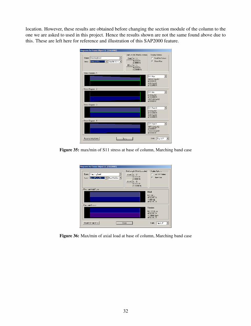
location. However, these results are obtained before changing the section module of the column to theone we are asked to used in this project. Hence the results shown are not the same found above due tothis. These are left here for reference and illustration of this SAP2000 feature.

Figure 35: max/min of S11 stress at base of column, Marching band case

Figure 36: Max/min of axial load at base of column, Marching band case

32

Figure 37: Max/min M22 at base of column, Marching band case

Figure 38: Max/min M33 at base of column, Marching band case

Figure 39: Stress S11 at base of column, Combination test case

33

Figure 40: Axial load at base of column, Combination test case

Figure 41: Max/min M22 at base of column, Combination test case

Figure 42: Max/min M33 at base of column, Combination test case

6.2 Method1. Selected run with all load cases.

34

2. Selected Display-Show Tables-Analysis Results-Element Output-Frame Output-Element ForcesModify/Show Options.. was used to make sure the envelope option is not selected and thatthe step-by-step option is selected under the Modal History Results. Also made sure thatthe load case MarchingBand and COMO are the only ones selected.

3. Waited for table to build. This took about 30 minutes. Then used the table filter to select column11 and station 0 (this is the bottom of the column).

4. Saved the table to a text file to process using Matlab. Here is the text file that contains the results.final_station_zero_forces.txt

5. Now obtained the stress due to dead load and dynamic load. This was done by running theanalysis again and now selecting LIVE and DEAD load cases and using the envelope. The resultis in this file final_load_result_DEAD_and_LIVE.txt

SAP2000 v15.0.1 5/8/13 2:08:08Table: Element Forces - Frames

Frame Station OutputCase CaseType P V2 V3 T M2 M3 S11Max PtS11Max x2S11Max x3S11Max S11Min PtS11Min x2S11Min x3S11Min FrameElem ElemStationft Kip Kip Kip Kip-ft Kip-ft Kip-ft Kip/ft2 ft ft Kip/ft2 ft ft ft

11 0.0000 DEAD LinStatic -101.634 0.257 -3.227 -6.3522 -19.2532 26.2485 -81.17 2 -0.50000 0.50000 -155.36 3 0.50000 -0.50000 11-1 0.000011 0.0000 LIVE LinStatic -40.210 0.082 -0.040 -1.4303 2.1635 14.0489 -34.51 1 -0.50000 -0.50000 -59.07 4 0.50000 0.50000 11-1 0.0000

6. Ran the Matlab script and obtained the maximum stress. The area for the column cross sectionis 0.8594 square ft. The matlab script is in this file stress_calc.m

7. Calculation used for stress is based on the following formula σ = PA ± M22

0.536 ±M33

0.586 Where A isthe section area of the beam and M22 and M33 are the internal bending moments at the base ofthe column obtained from SAP2000 finite elements results. Final stress was converted from kipper sq ft to kip per sq inch by dividing by 144.

35

7 Appendix

7.1 SAP2000 definitions used in this reportThese below are obtained from SAP2000 help sections.

7.1.1 Local axis signs

Figure 43: SAP2000 local axis signs

36

7.1.2 Frame element internal forces output convention

Figure 44: SAP2000 Frame element internal forces output convention

37

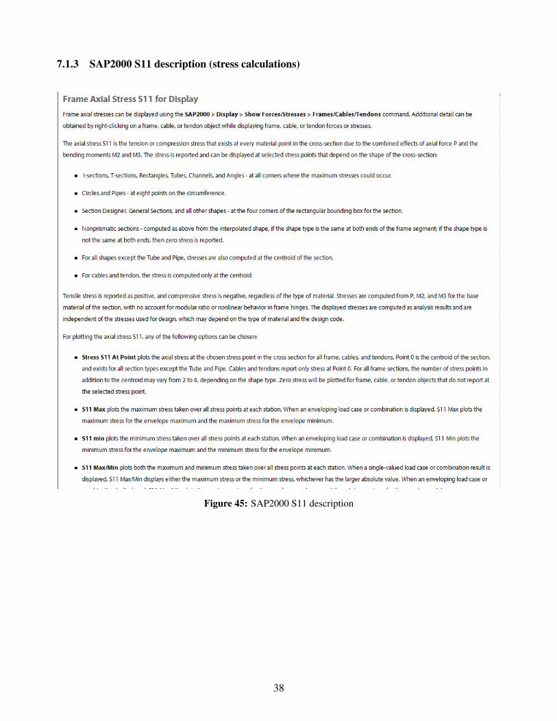
7.1.3 SAP2000 S11 description (stress calculations)

Figure 45: SAP2000 S11 description

38

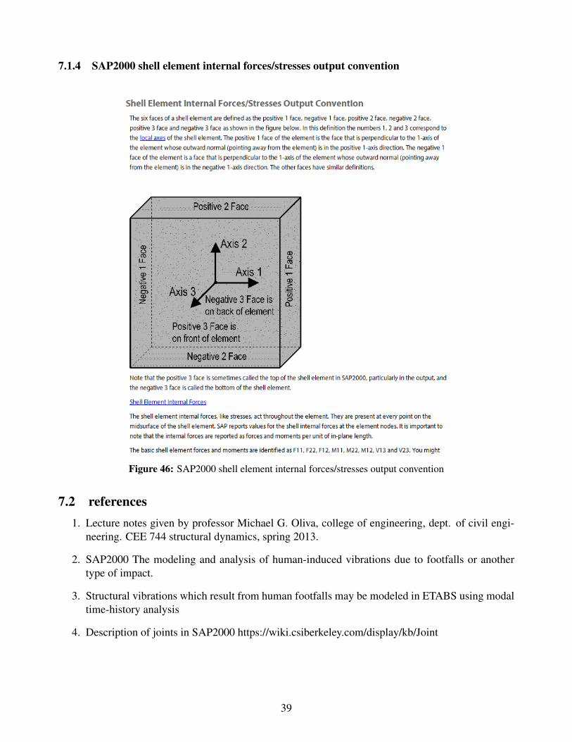
7.1.4 SAP2000 shell element internal forces/stresses output convention

Figure 46: SAP2000 shell element internal forces/stresses output convention

7.2 references1. Lecture notes given by professor Michael G. Oliva, college of engineering, dept. of civil engi-

neering. CEE 744 structural dynamics, spring 2013.

2. SAP2000 The modeling and analysis of human-induced vibrations due to footfalls or anothertype of impact.

3. Structural vibrations which result from human footfalls may be modeled in ETABS using modaltime-history analysis

4. Description of joints in SAP2000 https://wiki.csiberkeley.com/display/kb/Joint

39