55
DEMONSTRATION REPORT Advanced EMI Models for Live-site UXO Discrimination at Former Camp Beale ESTCP Project MR-201101 FEBRUARY 2012 Fridon Shubitidze Sky Research, Inc.
| Date post: | 05-Jun-2018 |
| Category: |
Documents |
| Upload: | duongthien |
| View: | 228 times |
| Download: | 2 times |

DEMONSTRATION REPORT Advanced EMI Models for Live-site UXO Discrimination at
Former Camp Beale
ESTCP Project MR-201101
FEBRUARY 2012
Fridon Shubitidze Sky Research, Inc.

Demonstration report Advanced EMI models for Camp Beale
MM ESTCP 201101 i February 2012
Table of Contents
1 INTRODUCTION............................................................................................................. 1
1.1 Background ............................................................................................................. 1
1.2 Brief site history ...................................................................................................... 2
1.3 Objective of the demonstration ............................................................................... 2
2 TECHNOLOGY ............................................................................................................... 3
2.1 The orthonormalized volume magnetic source model ............................................ 3
2.2 Joint diagonalization for data preprocessing........................................................... 4
2.3 EMI Data inversion: A global optimization technique ........................................... 5
2.3.1 Discrimination parameters .......................................................................... 5
2.3.2 Clustering of CBE anomalies...................................................................... 6
2.3.3 Classification using template matching ...................................................... 6
2.4 Details of classification schemes ............................................................................ 6
2.4.1 MetalMapper data inversion and classification scheme ............................. 6
2.4.2 2 2-3D-TEMTADS data sets data inversion and classification scheme 17
2.4.3 MPV-II data inversion and classification scheme .................................... 24
2.5 Brief chronological summary ............................................................................... 27
3 PERFORMANCE OBJECTIVES ................................................................................. 29
3.1 Objective: maximize correct classification of munitions ...................................... 29
3.1.1 Metric ........................................................................................................ 30
3.1.2 Data requirements ..................................................................................... 30
3.1.3 Success criteria evaluation and results ...................................................... 30
3.1.4 Results ....................................................................................................... 30
3.2 Objective: maximize correct classification of non-munitions .............................. 30
3.2.1 Metric ........................................................................................................ 30
3.2.2 Data requirements ..................................................................................... 30
3.2.3 Success criteria evaluation and results ...................................................... 31
3.2.4 Results ....................................................................................................... 31
3.3 Objective: specify a no-dig threshold ................................................................... 31
3.3.1 Metric ........................................................................................................ 31
3.3.2 Data requirements ..................................................................................... 31
3.3.3 Success criteria evaluation and results ...................................................... 31

Demonstration report Advanced EMI models for Camp Beale
MM ESTCP 201101 ii February 2012
3.3.4 Results ....................................................................................................... 31
3.4 Objective: minimize the number of anomalies that cannot be analyzed .............. 31
3.4.1 Metric ........................................................................................................ 32
3.4.2 Data requirements ..................................................................................... 32
3.4.3 Success criteria evaluation and results ...................................................... 32
3.4.4 Results ....................................................................................................... 32
3.5 Objective: correct estimation of target parameters ............................................... 32
3.5.1 Metric ........................................................................................................ 32
3.5.2 Data requirements ..................................................................................... 32
3.5.3 Success criteria evaluation and results ...................................................... 32
3.5.4 Results ....................................................................................................... 32
4 TEST DESIGN ................................................................................................................ 34
4.1 Site preparation ..................................................................................................... 34
4.2 Demonstration schedule ........................................................................................ 34
5 DATA ANALYSIS PLAN .............................................................................................. 35
5.1 Extracting target locations .................................................................................... 35
5.2 Extracting target intrinsic parameters ................................................................... 35
5.2.1 Single targets ............................................................................................. 35
5.2.2 Multi-target cases ...................................................................................... 35
5.3 Selection of intrinsic parameters for classification ............................................... 36
5.4 Training ................................................................................................................. 36
5.5 Classification......................................................................................................... 36
5.6 Decision memo ..................................................................................................... 37
6 COST ASSESSMENT .................................................................................................... 38
7 MANAGEMENT AND STAFFING ............................................................................. 39
8 REFERENCES ................................................................................................................ 40
9 APPENDICES ................................................................................................................. 42
9.1 Appendix A: Health and Safety Plan (HASP) ...................................................... 42
9.2 Appendix B: Points of Contact ............................................................................. 42
9.3 Appendix C: DATA Pre-processing and formatting for ONVMS code ............... 43
9.4 Run ONVMS code ................................................................................................ 46
9.5 Generate Custom Training Data list ..................................................................... 48

Demonstration report Advanced EMI models for Camp Beale
MM ESTCP 201101 iii February 2012
List of Figures
Figure 1. Camp Beale MM multi-static response matrix eigenvalues versus time for some
samples of requested anomalies. ..........................................................................................7
Figure 2. MM multi-static response matrix eigenvalues versus time for (top row) a 105-
mm projectile and an 81-mm mortar, (center row) a 60mm mortar and a 37-mm
munition, and (third row) an ISO target, and a fuze part. ....................................................8
Figure 3. Inverted total ONVMS time-decay profiles for an 81-mm mortar in the camp
Beale study, Anomaly #206. ................................................................................................9
Figure 4. Scatter plot of size and decay for all Camp Beale MM anomalies based on the
extracted total ONVMS for time channels Nos. 5, 10, 20, and 35. ...................................10
Figure 5. Result of the clustering for the Camp Beale MM anomalies using the size and
shape information for n = 35 (Figure 4). The circles denote the anomalies for
which the ground truth was asked. .....................................................................................11
Figure 6. TONVMS vs. time for some samples of Camp Beale MM anomalies. In the
delivered ground truth, Anomaly # 2228 was identified as a TOI. ....................................11
Figure 7. Inverted total ONVMS time-decay profiles for four targets: (top row) 105-mm
projectile and 81-mm mortar, and (bottom) 60-mm mortar and 37-mm projectile. ..........12
Figure 8. Inverted total ONSMS time decay profiles for ISO (excluded training ISOs )
targets and fuze parts. ........................................................................................................13
Figure 9. ROC curves for CH2MHILL Camp Beale MM data sets. The results were
obtained by the Sky Research R&D team using library-matching and statistical
classification approaches. In (a) it is assumed that fuzes are clutter; in (b) they are
considered TOI...................................................................................................................14
Figure 10. ROC curve for Parsons Camp Beale MM data sets. The results were obtained
by the Sky Research production team using library-matching classification. In a)
fuzes are considered clutter; in b) fuzes are assumed to be TOI. ......................................16
Figure 11. Camp Beale 2 2 MRS data matrix eigenvalues versus time for an ISO and a
37-mm; first row for single targets; the second row for two targets. .................................17
Figure 12. Camp Beale 2 2 MRS data matrix eigenvalues versus time for a 60-mm, an
81-mm, and magnetic soil. .................................................................................................18
Figure 13. Camp Beale 2 2 TEMATDS MRS data matrix eigenvalues versus time for
Test Case 758. ....................................................................................................................19
Figure 14. Total ONSMS for the 3-cm fuze part from Test Case-758 extracted using a
five-target inversion code. .................................................................................................20
Figure 15. Scatter plot of size (log10[TONVMSzz(t1))]) and decay
(log10[TONVMSzz(t1)/TONVMSzz(t80)]) for all Camp Beale 2 2 TEMTADS
anomalies based on the extracted total ONVMS. ..............................................................21

Demonstration report Advanced EMI models for Camp Beale
MM ESTCP 201101 iv February 2012
Figure 16. Result of the supervised clustering classification for the Camp Beale 2 2
TEMTADS anomalies using the size and shape information Figure 15. ..........................21
Figure 17. Total ONVMS versus time decay for Camp Beale 2 2 TEMATDS 105-mm,
81-mm, 60-mm and 37-mm TOI. ......................................................................................22
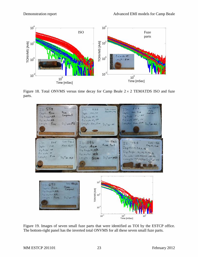
Figure 18. Total ONVMS versus time decay for Camp Beale 2 2 TEMATDS ISO and
fuze parts. ...........................................................................................................................23
Figure 19. Images of seven small fuze parts that were identified as TOI by the ESTCP
office. The bottom-right panel has the inverted total ONVMS for all these seven
small fuze parts. .................................................................................................................23
Figure 20. Camp Beale 2 2 TEMATDS anomalies ROC curve: a) fuzes as clutters; b)
fuzes as TOI. ......................................................................................................................24
Figure 21. Total ONVMS versus time for Camp Beale MPV-TD 105-mm, 81-mm, 60-
mm 37-mm, and ISO munitions and for the fuze parts identified as TOI by
ESTCP................................................................................................................................26
Figure 22. Inverted total ONVMS versus time for some of the small fuze parts identified
as TOI by the ESTCP office. .............................................................................................27
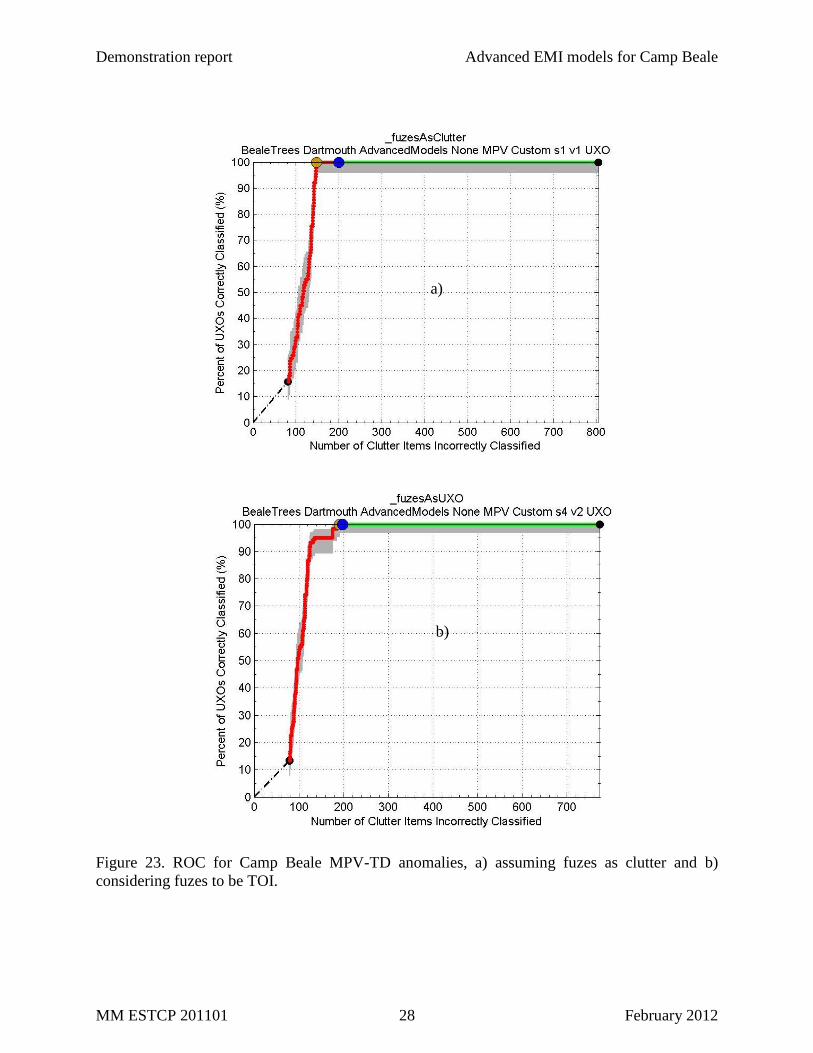
Figure 23. ROC for Camp Beale MPV-TD anomalies, a) assuming fuzes as clutter and b)
considering fuzes to be TOI. ..............................................................................................28
Figure 24 Histogram of depth errors (defined as | Z estimated
Zdata
| ) for the set of Camp
Beale CH2NHILL MetalMapper anomalies. The distribution shown has a mean of
4.07 cm and a standard deviation of 5.03 cm. There is good agreement between
the estimates and the ground truth. ....................................................................................33
Figure 25 Histogram of depth errors (defined as | Z estimated
Zdata
| ) for the set of Camp
Beale portable instruments anomalies. The depth errors distributions are shown
for 2x2 TEMTADS (left) and MPV-II (right) instruments , which have means of
4.97 cm and 4.62 cm, and standard deviations of 4.35 and 4.2 cm, respectively. ............33
Figure 26. Gantt chart showing a detailed schedule of the activities conducted at Camp
Beale. .................................................................................................................................34
Figure 27: Project management hierarchy. ....................................................................................39

Demonstration report Advanced EMI models for Camp Beale
MM ESTCP 201101 v February 2012
List of Tables
Table 1: Performance objectives ....................................................................................................29
Table 2: Cost model for advanced EMI model demonstration at the former Camp Beale ............38
Table 3: Points of Contact for the advanced EMI models demonstration. ....................................42

Demonstration report Advanced EMI models for Camp Beale
MM ESTCP 201101 vi February 2012
List of Acronyms
AIC Akaike Information Criterion
APG Aberdeen Proving Ground
BIC Bayesian Information Criterion
BUD Berkeley UXO Discriminator
cm Centimeter
DLL Dynamic Link Libraries
DoD Department of Defense
EM Electromagnetic
EMA Expectation Maximization Algorithm
EMI Electromagnetic Induction
ESTCP Environmental Security Technology Certification Program
FCS Former Camp Sibert
GSEA Generalized standardized excitation approach
IDA Institute for Defense Analyses.
ISO Industry Standard Object
JD Joint Diagonalization
MEG Magneto encephalographic
ML Maximum Likelihood
s Microsecond
mm Millimeter
MM MetalMapper
MPV Man-Portable Vector
ms Millisecond
MR Munitions response
MSR Multi-static response
MUSIC Multiple Signal Classification
NC North Carolina
NSMS Normalized surface magnetic source
NV/SMS Normalized volume or surface magnetic source models
ONVMS Orthogonal normalized volume magnetic source
ONV/SMS Orthonormalized volume or surface magnetic source models
PNN Probabilistic Neural Network
ROC Receiver Operating Characteristic
SERDP Strategic Environmental Research and Development Program
SLO San Luis Obispo
SVM Support vector machine
TD Time Domain
TEMTADS Time Domain Electromagnetic Towed Array Detection System
TOI Target of Interest
UXO Unexploded Ordnance

Demonstration report Advanced EMI models for Camp Beale
MM ESTCP 201101 1 February 2012
1 INTRODUCTION
This demonstration report is designed to illustrate the discrimination performance at an actual
UXO live-site of a set of advanced models for the analysis and inversion of electromagnetic
induction (EMI) data that go far beyond the popular but often inadequate simple dipole scheme.
The suite of methods, which combines the orthonormalized volume magnetic source (ONVMS)
model, a data-preprocessing technique based on joint diagonalization (JD), and differential
evolution (DE) minimization, among others, was tested at the former Camp Beale in California.
The partially wooded site is contaminated with a mix of 37-mm, 60-mm, 81-mm, and 105-mm
munitions, as well as complete and partial fuzes. For brevity we abstain from repeating
demonstration- and site-specific information already presented elsewhere; the interested reader
may turn to the ESTCP Live Site Demonstration Plan [1] and similar documents for
enlightenment on these topics.
1.1 Background
The Environmental Security Technology Certification Program (ESTCP) recently launched a
series of live-site UXO blind tests taking place in increasingly challenging and complex sites
[1],[2]. The first classification study was conducted in 2007 at the UXO live-site at the former
Camp Sibert in Alabama using two commercially available first-generation EMI sensors (the
EM61-MK2 and the EM-63, both from Geonics). At this site, the discrimination test was
relatively simple: one had to discriminate large intact 4.2 mortars from smaller range scrap,
shrapnel and cultural debris, and the anomalies were very well separated.
The second ESTCP discrimination study took place in 2009 at the live-UXO site at Camp San
Luis Obispo (SLO) in California and featured a more challenging topography and a wider mix of
targets of interest (TOI) [2]. Magnetometers and first-generation EMI sensors (again the Geonics
EM61-MK2) were deployed on the site and used in survey mode for a first screening.
Afterwards, two advanced EMI sensing systems—the Berkeley UXO Discriminator (BUD) and
the Naval Research Laboratory’s TEMTADS array—were used to perform cued interrogation of
a number of the anomalies detected. A third advanced system, the Geometrics MetalMapper, was
used in both survey and cued modes for anomaly identification and classification. Among the
munitions buried at SLO were 60-mm, 81-mm, and 4.2 mortars and 2.36 rockets; three
additional types of munitions were discovered during the course of the demonstration.
The third site chosen was the former Camp Butner in North Carolina. This demonstration was
designed to investigate evolving classification methodologies at a site contaminated with small
UXO targets, such as 37-mm projectiles.
The next site to be chosen for an ESTCP blind test was the former Camp Beale, whose roughly
60,000 acres straddle Yuba and Nevada Counties in California [1]. The demonstration was
conducted in a 10-acre area located within the historical bombing and the Toss Bomb target area
using several advanced EMI sensors, both handheld (MPV-II and 2 2-3D TEMTADS) and
cart-based (MetalMapper). The site was selected because it is partially wooded and because it
contains a wide mixture of TOI (including ISO, 37-mm, 60-mm, 81-mm, and 105-mm UXO) and
fuzes and fuze parts that could be considered TOI on some sites. These two features, plus the
magnetically responding soils encountered at the camp, are common occurrences in production

Demonstration report Advanced EMI models for Camp Beale
MM ESTCP 201101 2 February 2012
sites and add yet another layer of complexity into the classification process, providing additional
opportunities to demonstrate the capabilities and limitations of the advanced EMI models at
performing classification under a variety of site conditions.
1.2 Brief site history
Please refer to the ESTCP Live Site Demonstration Plan [1].
1.3 Objective of the demonstration
The advanced EMI models used for the analysis were developed under SERDP Project
MM-1572 and used with great success in the previous ESTCP tests [2],[4],[5],[6] and on data
collected at the Aberdeen Proving Ground (APG) in Maryland. In order to improve and
demonstrate the robustness and reliability of the models for live-site UXO discrimination,
however, one must keep putting them to the test at progressively challenging sites and for an
increasing number of next-generation EMI instruments sensors. The principal objectives of this
project are thus to apply advanced EMI models to UXO discrimination on actual live sites and to
demonstrate their classification capability in real-world scenarios. The specific technical
objectives are to:
1. Demonstrate the discrimination capability of the advanced EMI models for live-site
conditions;
2. Invert for target intrinsic parameters and use these to identify robust classification
features that may help distinguish UXO from non-hazardous objects; in other words, the
technology should
a. Indentify all seeded and native UXO;
b. Discard at least 75% of non-TOI targets;
3. Indentify sources of uncertainty in the classification process and incorporate them into
the dig/no-dig decision process;
4. Understand and document the applicability and limitations of the advanced EMI
discrimination technologies in the context of project objectives, site characteristics, and
suspected ordnance contamination.

Demonstration report Advanced EMI models for Camp Beale
MM ESTCP 201101 3 February 2012
2 TECHNOLOGY
The advanced EMI models and statistical signal processing approaches developed and tested
over the past three years under SERDP Project MM-1572 were able to detect and identify buried
UXO ranging in caliber from 25 mm up to 155 mm. The technique was seen to be physically
complete, fast, accurate, and clutter-tolerant, and provided excellent classification in both single-
and multiple-target scenarios when combined with multi-axis/transmitter/receiver sensors like
TEMTADS and the MetalMapper [3]. The methodology, augmented to include a suite of
classifiers, was also adapted to handheld sensors like the MPV and the 2 2-3D TEMTADS [7].
In this section we describe the different techniques one by one.
2.1 The orthonormalized volume magnetic source model
The advanced models we have developed for UXO discrimination include the normalized
surface magnetic source (NSMS) model [28] and the orthonormalized volume magnetic source
(ONVMS) model [13]. The NSMS procedure can be considered as a generalized surface dipole
model: in it, an object’s response to a sensor is modeled mathematically using a set of equivalent
pointlike analytic solutions of the Maxwell equations (usually dipoles, though charges are also a
possibility) distributed over a surface surrounding the object. The amplitudes of the sources are
proportional to the component of the primary magnetic field normal to the surface; once this
dependence is normalized out, the NSMS strengths can be determined directly by solving a
linear system of equations that results from minimizing the mismatch between measured and
modeled data for a known object-sensor combination.
The ONVMS model, a further extension of NSMS, posits that the entire scatterer can be replaced
with a set of magnetic dipole sources distributed over a computational volume. We make the
usual EMI assumptions: we neglect displacement currents and electric fields and conduction
currents in air and soil. The primary magnetic field established by the sensor penetrates the
objects in its vicinity to some degree, inducing eddy currents and magnetic dipoles inside them
which in turn produce a secondary or scattered magnetic field. This is the field that we propose
to represent as due to a volumetric distribution of magnetic dipole density:
sc
3
1 ˆ ˆ( , ) (3 ) ( , ) = ( , ) ( , ) 4
v v
V V
p p dv G p dvR
H r RR I m r r r m r , (1)
where p {t, f } is time or frequency, R̂ is the unit vector along R r rv
, rv
is the position
of the v -th infinitesimal dipole in the volume V, r is the observation point, and I and G(r, r )
are respectively the identity and Green dyads. The induced magnetic dipole moment m(rv, p) at
point rv on the surface is related to the primary field through m(r
, p) M(r
v, p) Hpr (r
v) ,
where M(rv, p) is the symmetric polarizability tensor. The secondary magnetic field at any
point can be expanded in a set of orthonormal functions i(r) as

Demonstration report Advanced EMI models for Camp Beale
MM ESTCP 201101 4 February 2012
H(r) i(R
i) b
ii1
Nv
, (2)
where we have also introduced the expansion coefficients bi. The
i are linear combinations of
dipole Green dyads guaranteed to be orthonormal by the Gram–Schmidt process; thanks to this
property the amplitudes of the tensor elements of Mi( p) can be determined without having to
solve a linear system of equations. The great advantages of ONVMS are that it takes into account
the mutual couplings between different sections of the targets and that it avoids matrix
singularity problems in multi-object cases. It treats single- and multi-target scenarios on the same
footing. Once the tensor elements and locations of the responding dipoles are determined one can
group them within the volume and for each group calculate the total polarizability, which at the
end is joint-diagonalized. These diagonal elements have been shown to be intrinsic to the objects,
and can be used, either on their own or in combination with other quantities, in discrimination
processing [6].
2.2 Joint diagonalization for data preprocessing
EMI sensors currently feature multi-axis illumination of targets and tri-axial vector sensing, or
exploit multi-static array data acquisition [1]–[6]. To take advantage of the rich data sets that
these sensors provide, we recently developed and successfully demonstrated a discrimination
procedure based on joint diagonalization [15]. To illustrate the application of JD to advanced
EMI sensors, we proceed to describe its implementation for the MetalMapper [3]. The system
consists of K = 3 mutually perpendicular transmitters and M = 7 triaxial receivers. The sensor
activates the transmitter loops in sequence, one at a time, and for each transmitter all receivers
measure the complete transient response over a wide dynamic range of time, approximately from
100 microseconds (s) to 8 milliseconds (ms), over 45 time gates. The sensor thus provides
3 21 spatial data points for any given time channel tq, q = 1, 2,…, Nq, where Nq is the number
of the time channels. If we define Hk ,m{zyx}
as the z, y, or x-component of the magnetic field
measured by the m-th receiver coil when the k-th transmitter is active, then the K 3M matrix
1,1 1,1 1,1 1,7 1,7 1,7
2,1 2,1 2,1 2,7 2,7 2,7
3,1 3,1 3,1 3,7 3,7 3,7
( )
z y x z y x
q z y x z y x
z y x z y x
H H H H H H
H t H H H H H H
H H H H H H
(3)
will be a set of measured data vectors for the k-th transmitter for each time channel. One can then
construct a new matrix B(tq) HT (t
q) H(t
q) again for each time channel, and, through an eigen-
decomposition, express it in terms of a diagonal matrix D(tq) of eigenvalues and an orthogonal
matrix U (tq) of eigenvectors:
B(tq) U(t
q) D(t
q) U T (t
q) , (4)

Demonstration report Advanced EMI models for Camp Beale
MM ESTCP 201101 5 February 2012
where T denotes the transpose. In order to relate the time-dependent eigenvalues to the number
of potential targets we find a single set V of eigenvectors that will be shared by all {B(tq)}
q1
Nq
matrices and will also make all their off-diagonal elements as vanishingly small as possible:
D(tq)
q1
Nq
V T B(tq)
q1
Nq
V . (5)
The technique that finds an orthogonal (i.e., real and unitary) matrix V that minimizes the
{B(tq)}
q1
Nq matrices’ off-diagonal elements is called “joint diagonalization” (JD) [15]. The
diagonal matrices {D(tq)}
q1
Nq contain information about the targets that contribute to the signal.
Our studies show that each set of three above-threshold diagonal elements of the measured multi-
static response (MSR) data matrix describe one target. We have also demonstrated that the JD
technique is a robust technique for extracting target signals in cases with a low signal-to-noise-
ratio. In addition, the eigenvalues’ time dependence exhibits the different targets’ classification
features [14].
2.3 EMI Data inversion: A global optimization technique
Determining a buried object’s orientation and location is a non-linear problem. Inverse-scattering
problems are solved by determining an objective function [14] as a goodness-of-fit measure
between modeled and measured magnetic field data. Standard gradient search approaches often
suffer from a surfeit of local minima that sometimes result in incorrect estimates for location and
orientation. To avoid this problem we recently developed a different class of global optimization
search algorithms. One such technique is the Differential Evolution (DE) method [26]–[27], a
heuristic, parallel, direct-search method for minimizing non-linear functions of continuous
variables that is very easy to implement and has good convergence properties. We combined DE
with ONVMS to invert digital geophysical EMI data [6]. All EMI optimizations were split into
linear and nonlinear parts, iterating between them to minimize the objective function. Once the
target locations are found, the amplitudes of responding ONVMS are determined and used to
classify the object relative to items of interest.
2.3.1 Discrimination parameters
To classify targets in this demonstration we used ONVMS combined with DE optimization and
joint diagonalization to invert for the locations of the targets of interest (TOI). The model
provides at least three independent total ONVMS parameters along the principal axis for each
potential target that can be used for discrimination. During the inversion stage the total time-
dependent ONVMS, which depends on the size, geometry, and material composition of the
object in question, is determined for each potential target. Early time gates bring out the high-
frequency response to the shutdown of the exciting field; the induced eddy currents in this range
are superficial, and a large total ONVMS amplitude at early times correlates with large objects
and large surface area. At late times, when the eddy currents have diffused completely into the
object and low-frequency harmonics dominate, the EMI response relates to the metal content
(i.e., the volume) of the target. Thus a smaller but compact object has a relatively weak early
response that dies down slowly, while a large but thin or hollow object has a strong initial

Demonstration report Advanced EMI models for Camp Beale
MM ESTCP 201101 6 February 2012
response that decays quickly. These parameters can be used to form feature vectors for
classification.
The success of classification depends on the selection of features, the separation of
different classes in feature space, and the ability of the sensor data to constrain the estimated
features. In some cases, due to poor signal-to-noise ratio, the feature vectors from UXO targets
can be corrupted or could be similar with clutter anomalies. In such cases, we must recognize
that discrimination may be limited or classification decision will require an override using an
expert’s judgment. When discrimination is possible we use both template-matching and
statistical procedures—such as Gaussian Mixture models, support vector machines (SVM) [17],
or probabilistic neural networks (PNN) [22]—since no single classifier is likely to be applicable
under all conditions [16].
2.3.2 Clustering of CBE anomalies
The distribution of power-law/exponential-decay parameters extracted from the total ONVMS
profiles is key to performing classification. This is because TOI with similar total ONVMS are
likely to show similar patterns under various conditions. By comparing the total ONVMS time-
decay parameters of unknown targets to those of known objects one can predict the class/cluster
to which the unknown targets belong. There are many clustering techniques available, such as K-
means [18], Principal Component Analysis [24], and Support Vector Machines [16].
2.3.3 Classification using template matching
The template matching technique is a classification approach that discriminates unknown targets
from TOI by comparing the extracted target’s features—in our case the total ONVMS—to a set
stored in library. There are two ways to execute the template-matching technique: 1) using code
that will estimate least-square mismatches between the unknown and library targets ONVMS,
and 2) by visual inspection. Since in the case of Camp Beale there were unexpected TOI (whole
and partial fuzes), we used both approaches when classifying the targets.
2.4 Details of classification schemes
The discrimination process comprises three sequential tasks: data collection, data inversion, and
classification. Each EMI sensor produces unique data sets and therefore requires its own data
inversion and classification schemes. This section summarizes the data inversion and
classification schemes for the MetalMapper, the 2 2-3D TEMTADS array, and the MPV
sensor.
2.4.1 MetalMapper data inversion and classification scheme
The MM sensor’s Tx and Rx signals detailed modeling approach using the ONVMS-DE
algorithm is described in [14].
Step 1. Data pre-processing: All MM-data were pre-processed using a Matlab Code (see
Appendix 9.3). The code reads comma-delimited format CSV files and transfers them to
ASCII files compatible with the ONVMS-DE code (ONVMS_MM.exe). The user needs only
specify the path to the folder with the CSV files; the code then converts them all.
Demonstration report Advanced EMI models for Camp Beale
MM ESTCP 201101 7 February 2012
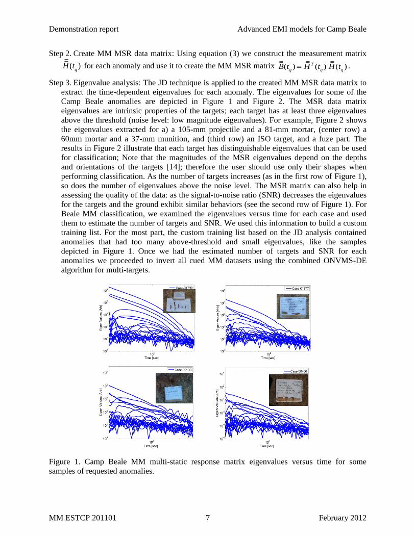
Step 2. Create MM MSR data matrix: Using equation (3) we construct the measurement matrix
H(tq) for each anomaly and use it to create the MM MSR matrix B(t
q) HT (t
q) H(t
q) .
Step 3. Eigenvalue analysis: The JD technique is applied to the created MM MSR data matrix to
extract the time-dependent eigenvalues for each anomaly. The eigenvalues for some of the
Camp Beale anomalies are depicted in Figure 1 and Figure 2. The MSR data matrix
eigenvalues are intrinsic properties of the targets; each target has at least three eigenvalues
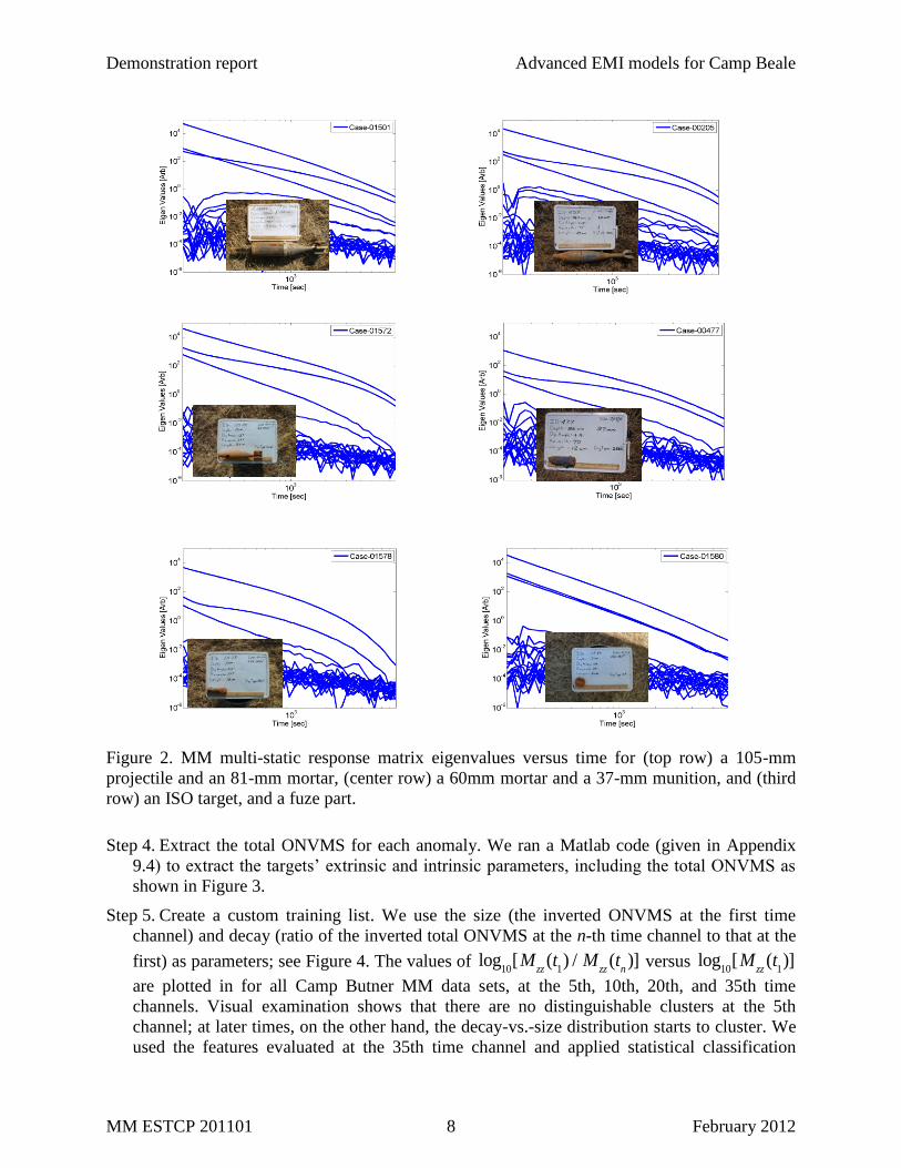
above the threshold (noise level: low magnitude eigenvalues). For example, Figure 2 shows
the eigenvalues extracted for a) a 105-mm projectile and a 81-mm mortar, (center row) a
60mm mortar and a 37-mm munition, and (third row) an ISO target, and a fuze part. The
results in Figure 2 illustrate that each target has distinguishable eigenvalues that can be used
for classification; Note that the magnitudes of the MSR eigenvalues depend on the depths
and orientations of the targets [14]; therefore the user should use only their shapes when
performing classification. As the number of targets increases (as in the first row of Figure 1),
so does the number of eigenvalues above the noise level. The MSR matrix can also help in
assessing the quality of the data: as the signal-to-noise ratio (SNR) decreases the eigenvalues
for the targets and the ground exhibit similar behaviors (see the second row of Figure 1). For
Beale MM classification, we examined the eigenvalues versus time for each case and used
them to estimate the number of targets and SNR. We used this information to build a custom
training list. For the most part, the custom training list based on the JD analysis contained
anomalies that had too many above-threshold and small eigenvalues, like the samples
depicted in Figure 1. Once we had the estimated number of targets and SNR for each
anomalies we proceeded to invert all cued MM datasets using the combined ONVMS-DE
algorithm for multi-targets.
Figure 1. Camp Beale MM multi-static response matrix eigenvalues versus time for some
samples of requested anomalies.
Demonstration report Advanced EMI models for Camp Beale
MM ESTCP 201101 8 February 2012
Figure 2. MM multi-static response matrix eigenvalues versus time for (top row) a 105-mm
projectile and an 81-mm mortar, (center row) a 60mm mortar and a 37-mm munition, and (third
row) an ISO target, and a fuze part.
Step 4. Extract the total ONVMS for each anomaly. We ran a Matlab code (given in Appendix
9.4) to extract the targets’ extrinsic and intrinsic parameters, including the total ONVMS as
shown in Figure 3.
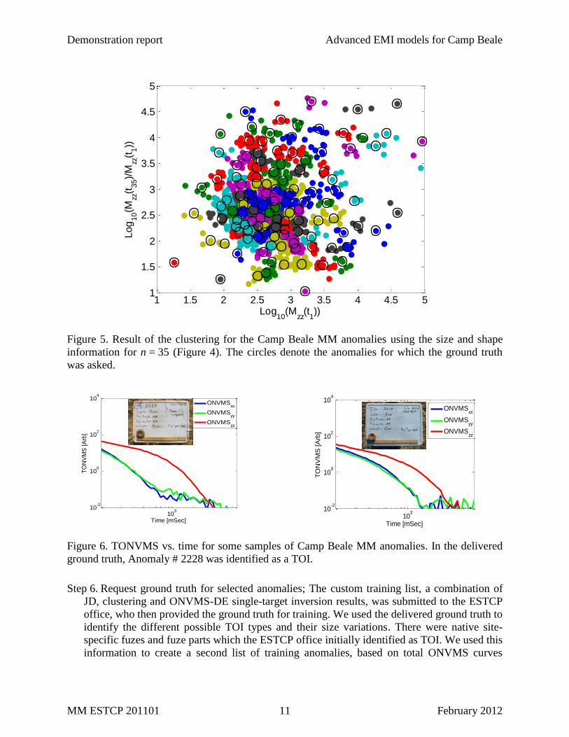
Step 5. Create a custom training list. We use the size (the inverted ONVMS at the first time
channel) and decay (ratio of the inverted total ONVMS at the n-th time channel to that at the
first) as parameters; see Figure 4. The values of log10
[Mzz
(t1) / M
zz(t
n)] versus log
10[M
zz(t
1)]
are plotted in for all Camp Butner MM data sets, at the 5th, 10th, 20th, and 35th time
channels. Visual examination shows that there are no distinguishable clusters at the 5th
channel; at later times, on the other hand, the decay-vs.-size distribution starts to cluster. We
used the features evaluated at the 35th time channel and applied statistical classification

Demonstration report Advanced EMI models for Camp Beale
MM ESTCP 201101 9 February 2012
techniques. The Matlab code that uses the inverted ONVMS for clustering is given in
Appendix 9.5; it also uses Matlab’s built-in function “clusterdata”. In this studies the size
(log10(TONVMSzz(t1))) and decay (log10(TONVMSzz(t1) / TONVMSzz(tn))) parameters for n = 35 are
used for clustering and the number of clusters is 8% of the total number of anomalies. For
each cluster we computed the centroid and determined the anomaly closest to it. This
anomaly we included in the custom training data list (see the Matlab code in Appendix 9.5).
The clustering results are depicted in Figure 5. Each color corresponds to a cluster; circles
denote anomalies for which the ground truth was asked. In addition to the statistical
clustering algorithm, ONVMS time decay curves were inspected for each anomaly: we used
the TONVMS time decay shapes and symmetries to further validate or modify the custom
training anomaly list. Anomalies with significantly asymmetric TONVMS were removed
from the training list; anomalies with fast decay but symmetric profiles were added to the
training list for which we requested the identifying ground truth. Some samples of such
anomalies are shown in Figure 6.
Figure 3. Inverted total ONVMS time-decay profiles for an 81-mm mortar in the camp Beale
study, Anomaly #206.
103
10-2
10-1
100
101
102
103
104
Case-206
Time [mSec]
TO
NV
MS
[A
rb]
Total ONVMSxx
Total ONVMSyy
Total ONVMSzz
TONVMSzz(t1) Size
TONVMSzz(tn) Decay

Demonstration report Advanced EMI models for Camp Beale
MM ESTCP 201101 10 February 2012
Figure 4. Scatter plot of size and decay for all Camp Beale MM anomalies based on the extracted
total ONVMS for time channels Nos. 5, 10, 20, and 35.
1 2 3 4 5 60
0.5
1
1.5
2
2.5
3
Log10
(Mzz
(t1))
Log
10(M
zz(t
20)/
Mzz(t
1))
1 2 3 4 5 6-0.5
0
0.5
1
1.5
2
2.5
Log10
(Mzz
(t1))
Log
10(M
zz(t
10)/
Mzz(t
1))
1 2 3 4 5 6-0.5
0
0.5
1
1.5
2
Log10
(Mzz
(t1))
Log
10(M
zz(t
5)/
Mzz(t
1)) n=5
n=10
1 1.5 2 2.5 3 3.5 4 4.5 51
1.5
2
2.5
3
3.5
4
4.5
5
Log10
(Mzz
(t1))
Log
10(M
zz(t
35)/
Mzz(t
1))
n=35 n=20
Demonstration report Advanced EMI models for Camp Beale
MM ESTCP 201101 11 February 2012
1 1.5 2 2.5 3 3.5 4 4.5 51
1.5
2
2.5
3
3.5
4
4.5
5
Log10
(Mzz
(t1))
Log
10(M
zz(t
35)/
Mzz
(t1))
Figure 5. Result of the clustering for the Camp Beale MM anomalies using the size and shape
information for n = 35 (Figure 4). The circles denote the anomalies for which the ground truth
was asked.
Figure 6. TONVMS vs. time for some samples of Camp Beale MM anomalies. In the delivered
ground truth, Anomaly # 2228 was identified as a TOI.
Step 6. Request ground truth for selected anomalies; The custom training list, a combination of
JD, clustering and ONVMS-DE single-target inversion results, was submitted to the ESTCP
office, who then provided the ground truth for training. We used the delivered ground truth to
identify the different possible TOI types and their size variations. There were native site-
specific fuzes and fuze parts which the ESTCP office initially identified as TOI. We used this
information to create a second list of training anomalies, based on total ONVMS curves
103
10-2
100
102
104
Time [mSec]
TO
NV
MS
[A
rb]
ONVMSxx
ONVMSyy
ONVMSzz
103
10-2
100
102
104
Time [mSec]
TO
NV
MS
[A
rb]
ONVMSxx
ONVMSyy
ONVMSzz
Demonstration report Advanced EMI models for Camp Beale
MM ESTCP 201101 12 February 2012
obtained using a multi-target inversion code, which we again submitted to ESTCP. The
ground truth for the second list indicated that there were fuzes of varying size and material
composition. We further examined the ONVMS-DE multi-target cases and produced a third
anomaly list that was submitted to the ESTCP office.
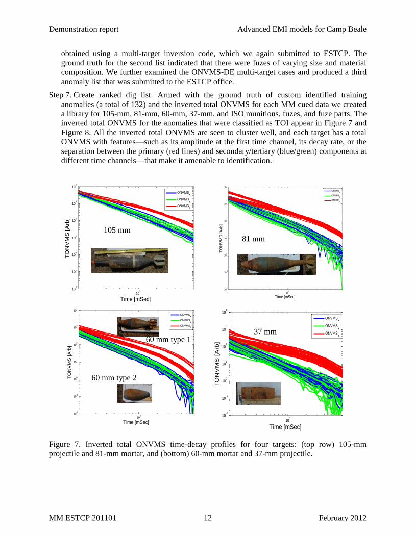
Step 7. Create ranked dig list. Armed with the ground truth of custom identified training
anomalies (a total of 132) and the inverted total ONVMS for each MM cued data we created
a library for 105-mm, 81-mm, 60-mm, 37-mm, and ISO munitions, fuzes, and fuze parts. The
inverted total ONVMS for the anomalies that were classified as TOI appear in Figure 7 and
Figure 8. All the inverted total ONVMS are seen to cluster well, and each target has a total
ONVMS with features—such as its amplitude at the first time channel, its decay rate, or the
separation between the primary (red lines) and secondary/tertiary (blue/green) components at
different time channels—that make it amenable to identification.
Figure 7. Inverted total ONVMS time-decay profiles for four targets: (top row) 105-mm
projectile and 81-mm mortar, and (bottom) 60-mm mortar and 37-mm projectile.
103
10-2
10-1
100
101
102
103
104
Time [mSec]
TO
NV
MS
[A
rb]
ONVMSx
ONVMSy
ONVMSz
103
10-2
10-1
100
101
102
103
104
Time [mSec]
TO
NV
MS
[A
rb]
ONVMSx
ONVMSy
ONVMSz
103
10-2
10-1
100
101
102
103
104
Time [mSec]
TO
NV
MS
[A
rb]
ONVMSx
ONVMSy
ONVMSz
103
10-2
10-1
100
101
102
103
104
Time [mSec]
TO
NV
MS
[A
rb]
ONVMSx
ONVMSy
ONVMSz
105 mm 81 mm
60 mm type 2
60 mm type 1 37 mm
Demonstration report Advanced EMI models for Camp Beale
MM ESTCP 201101 13 February 2012
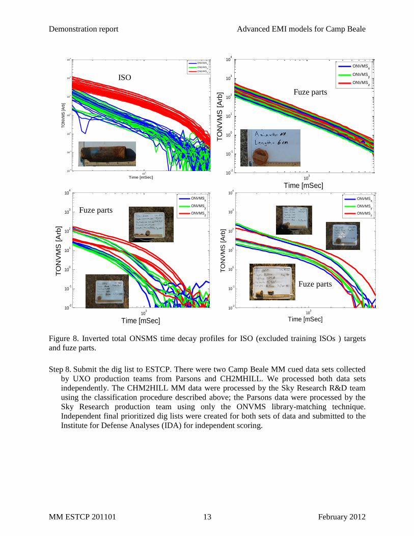
Figure 8. Inverted total ONSMS time decay profiles for ISO (excluded training ISOs ) targets
and fuze parts.
Step 8. Submit the dig list to ESTCP. There were two Camp Beale MM cued data sets collected
by UXO production teams from Parsons and CH2MHILL. We processed both data sets
independently. The CHM2HILL MM data were processed by the Sky Research R&D team
using the classification procedure described above; the Parsons data were processed by the
Sky Research production team using only the ONVMS library-matching technique.
Independent final prioritized dig lists were created for both sets of data and submitted to the
Institute for Defense Analyses (IDA) for independent scoring.
103
10-2
10-1
100
101
102
103
104
Time [mSec]
TO
NV
MS
[A
rb]
ONVMSx
ONVMSy
ONVMSz
103
10-2
10-1
100
101
102
103
104
Time [mSec]
TO
NV
MS
[A
rb]
103
10-2
10-1
100
101
102
103
104
Time [mSec]
TO
NV
MS
[A
rb]
ONVMSx
ONVMSy
ONVMSz
103
10-2
10-1
100
101
102
103
104
Time [mSec]
TO
NV
MS
[A
rb]
ONVMSx
ONVMSy
ONVMSz
103
10-2
10-1
100
101
102
103
104
Time [mSec]
TO
NV
MS
[Arb
]
ONVMSx
ONVMSy
ONVMSz
ISO
targets Fuze parts
Fuze parts
Fuze parts

Demonstration report Advanced EMI models for Camp Beale
MM ESTCP 201101 14 February 2012
Figure 9. ROC curves for CH2MHILL Camp Beale MM data sets. The results were obtained by
the Sky Research R&D team using library-matching and statistical classification approaches. In
(a) it is assumed that fuzes are clutter; in (b) they are considered TOI.
a)
b)

Demonstration report Advanced EMI models for Camp Beale
MM ESTCP 201101 15 February 2012
a) Camp Beale CH2MHILL MM data classification results
The IDA scored results for CH2MHILL MM 1470 anomalies in the form of a receiver operating
characteristic (ROC) curves are depicted in Figure 9 a) and Figure 9 b) assuming respectively
that fuzes are clutter and that they are TOI. The result shows that a) of the 132 targets that were
dug for training, 107 targets were not TOI (shift along x-axis) and 25 were (shift along y-axis);
b) there are no false negatives: all 170, of which 89 were UXO/ISO and 33 were fuzes, TOI were
correctly identified; c) to classify all TOI correctly only 65 extra (false positive) digs are needed;
d) for increased classification confidence the algorithm requested an additional eleven digs after
all TOI had been identified correctly, 1117 (~86 % of clutters out of 1300) were identified as
non-TOI with high confidence.
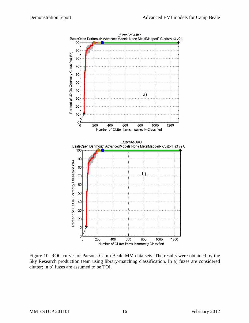
b) Camp Beale Parsons MM Data classification results
The Sky Research production team first inverted total ONVMS for potential TOI using testing
data collected at the site. They then visually compared the total ONVMS time-decay curves of
potential targets to those of the test anomalies. During the comparisons “suspicious” targets were
identified. The targets did not match any library targets yet exhibited UXO-like features, such as
potential BOR symmetry and slow decays. The “suspicious” anomalies were included in a list of
training anomalies whose ground truth was requested from the ESTCP office. The delivered
ground truth revealed two unexpected TOI fuze types that were added to the library. Using the
updated library, all targets were ranked as TOI and clutter; the dig list was created and submitted
to the IDA office for scoring. The resulting ROC curves are depicted in Figure 10 a) and b)
assuming fuzes to be respectively clutter and TOI. The result shows that a) of the 69 targets that
were dug for training, 50 were not TOI (shift along x-axis) and 19 were (shift along y-axis); b) no
false negatives: all TOI (a total of 170) were identified correctly; c) to classify all TOI correctly
only 203 extra (false positive) digs are needed; d) 1047 (~81 % of clutter items) were identified
as non-TOI with high confidence.
Demonstration report Advanced EMI models for Camp Beale
MM ESTCP 201101 16 February 2012
Figure 10. ROC curve for Parsons Camp Beale MM data sets. The results were obtained by the
Sky Research production team using library-matching classification. In a) fuzes are considered
clutter; in b) fuzes are assumed to be TOI.
a)
b)

Demonstration report Advanced EMI models for Camp Beale
MM ESTCP 201101 17 February 2012
2.4.2 2 2-3D-TEMTADS data sets data inversion and classification scheme
The 2 2 3D-TEMATDS area is a next-generation portable EMI system. The instrument’s
electronics, geometry, data collection procedure, and file formats are described in [6]. For the
Camp Beale 2 2-3D TEMATDS cued data we applied the inversion and classification protocol
described above for the MM data sets.
Step 1. Transfer all CSV files to an ASCII-based format compatible with the TEMATDS
ONVMS-DE code (ONVMS_2_2.exe).
Step 2. Construct the 2 2 TEMATDS MSR data matrix as described for MM.
Step 3. Apply JD to 2 2 TEMATDS MSR data matrix; extract eigenvalues versus time;
conduct eigenvalue analysis; determine data quality and number of potential targets in each
cell. The 2 2 TEMTADS MRS data matrix eigenvalues versus time for some camp Beale
anomalies are depicted in Figure 11 and Figure 12; featured are an ISO, a 37-mm, a 60-mm,
a 81-mm, and magnetic soil.
Figure 11. Camp Beale 2 2 MRS data matrix eigenvalues versus time for an ISO and a 37-mm;
first row for single targets; the second row for two targets.

Demonstration report Advanced EMI models for Camp Beale
MM ESTCP 201101 18 February 2012
Figure 12. Camp Beale 2 2 MRS data matrix eigenvalues versus time for a 60-mm, an 81-mm,
and magnetic soil.
The results show that the 2 2 TEMTADS MSR eigenvalues are intrinsic properties of the
targets. Each target has very distinguishable eigenvalues that stay the same even when the
signal is contaminated with signals from nearby targets (see Figure 11). We used the
eigenvalues’ characteristics directly to perform an initial classification. Figure 12 shows that
the MRS data matrix eigenvalues provide fast and robust information about the data quality.
For example, comparing Case-352 with Case-356 (Figure 12 second column) shows that
when the sensor is well positioned above the target the eigenvalues are strong and well above
the noise level; on the other hand, when the sensor is offset from the target the eigenvalues
become noisy and mix with those of the soil (see Figure 12 for Case-382). In order to avoid
misclassification, those anomalies were placed into the training data list. The results also
indicate that as the number of targets increases, so does the number of eigenvalues above the
noise level. The anomalies with a significant number of eigenvalues (> 6) above the noise
level were also included in the training data; the 2 2 TEMATDS MSR eigenvalues for one
such case are shown in Figure 13.
Demonstration report Advanced EMI models for Camp Beale
MM ESTCP 201101 19 February 2012
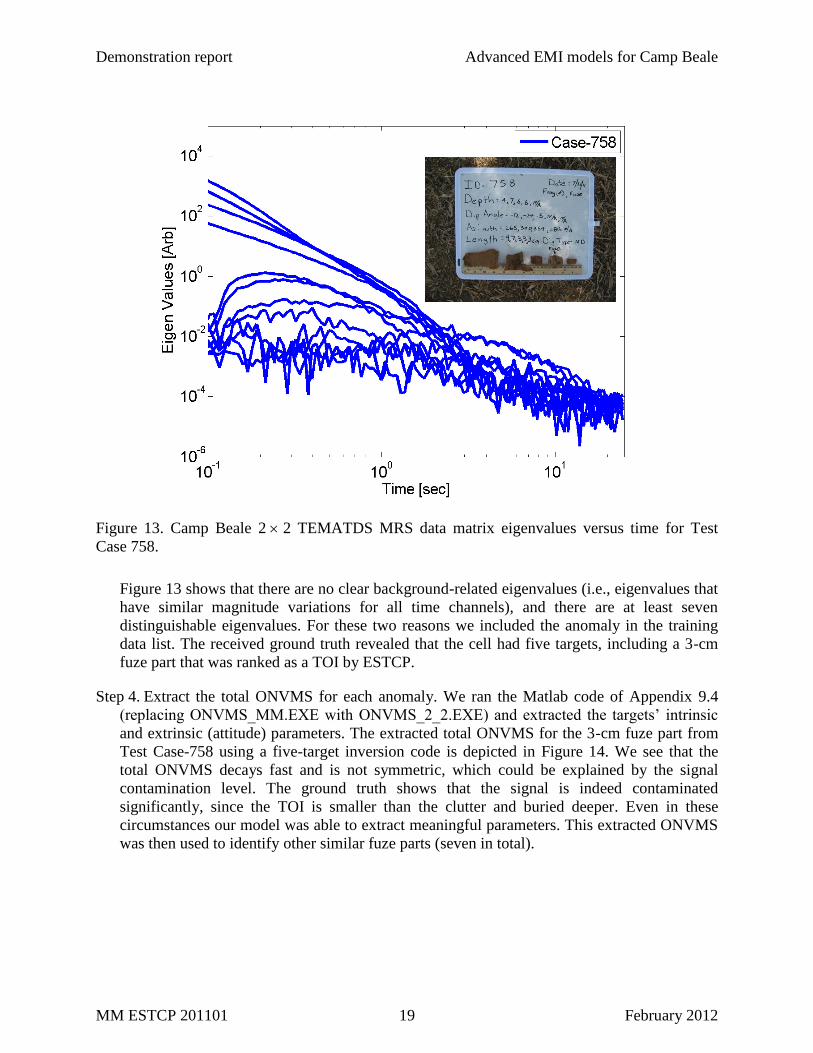
Figure 13. Camp Beale 2 2 TEMATDS MRS data matrix eigenvalues versus time for Test
Case 758.
Figure 13 shows that there are no clear background-related eigenvalues (i.e., eigenvalues that
have similar magnitude variations for all time channels), and there are at least seven
distinguishable eigenvalues. For these two reasons we included the anomaly in the training
data list. The received ground truth revealed that the cell had five targets, including a 3-cm
fuze part that was ranked as a TOI by ESTCP.
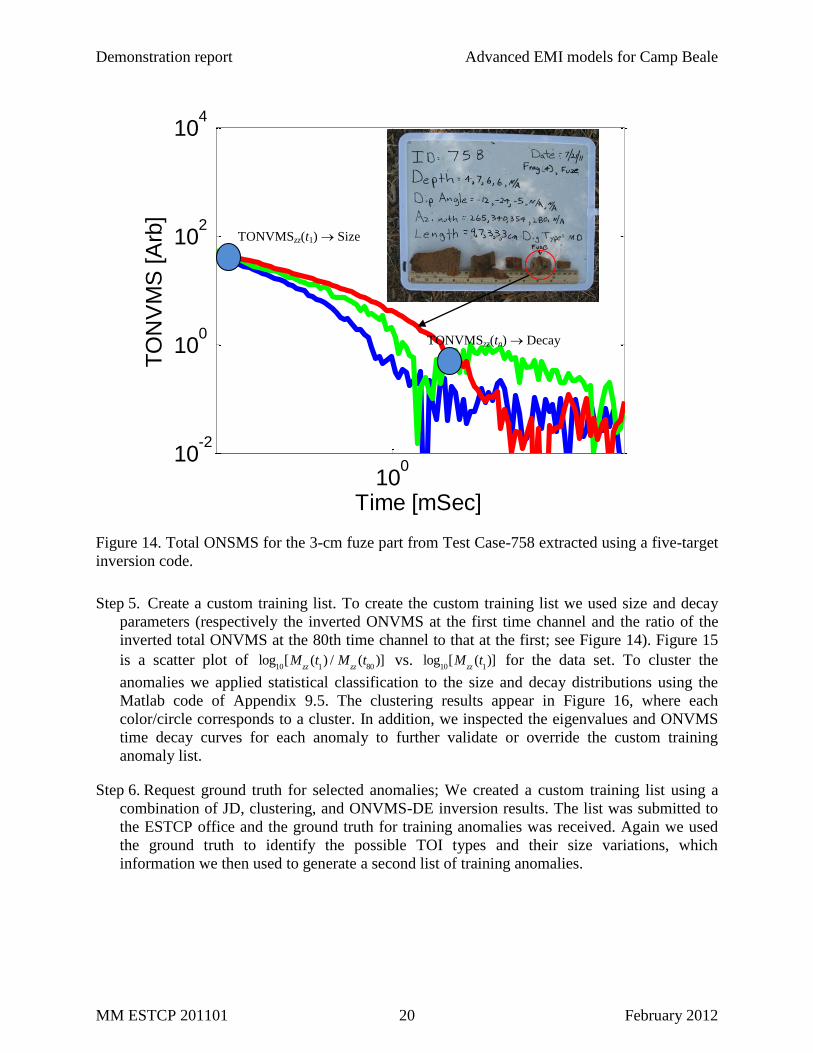
Step 4. Extract the total ONVMS for each anomaly. We ran the Matlab code of Appendix 9.4
(replacing ONVMS_MM.EXE with ONVMS_2_2.EXE) and extracted the targets’ intrinsic
and extrinsic (attitude) parameters. The extracted total ONVMS for the 3-cm fuze part from
Test Case-758 using a five-target inversion code is depicted in Figure 14. We see that the
total ONVMS decays fast and is not symmetric, which could be explained by the signal
contamination level. The ground truth shows that the signal is indeed contaminated
significantly, since the TOI is smaller than the clutter and buried deeper. Even in these
circumstances our model was able to extract meaningful parameters. This extracted ONVMS
was then used to identify other similar fuze parts (seven in total).
Demonstration report Advanced EMI models for Camp Beale
MM ESTCP 201101 20 February 2012
Figure 14. Total ONSMS for the 3-cm fuze part from Test Case-758 extracted using a five-target
inversion code.
Step 5. Create a custom training list. To create the custom training list we used size and decay
parameters (respectively the inverted ONVMS at the first time channel and the ratio of the
inverted total ONVMS at the 80th time channel to that at the first; see Figure 14). Figure 15
is a scatter plot of log10
[Mzz
(t1) / M
zz(t
80)] vs. log
10[M
zz(t
1)] for the data set. To cluster the
anomalies we applied statistical classification to the size and decay distributions using the
Matlab code of Appendix 9.5. The clustering results appear in Figure 16, where each
color/circle corresponds to a cluster. In addition, we inspected the eigenvalues and ONVMS
time decay curves for each anomaly to further validate or override the custom training
anomaly list.
Step 6. Request ground truth for selected anomalies; We created a custom training list using a
combination of JD, clustering, and ONVMS-DE inversion results. The list was submitted to
the ESTCP office and the ground truth for training anomalies was received. Again we used
the ground truth to identify the possible TOI types and their size variations, which
information we then used to generate a second list of training anomalies.
100
10-2
100
102
104
Time [mSec]
TO
NV
MS
[A
rb]
TONVMSzz(t1) Size
TONVMSzz(tn) Decay

Demonstration report Advanced EMI models for Camp Beale
MM ESTCP 201101 21 February 2012
0 1 2 3 4 5
0
1
2
3
4
5
Size
Decay
Figure 15. Scatter plot of size (log10[TONVMSzz(t1))]) and decay (log10[TONVMSzz(t1)/TONVMSzz(t80)])
for all Camp Beale 2 2 TEMTADS anomalies based on the extracted total ONVMS.
0 1 2 3 4 5
0
1
2
3
4
5
75
Size
Decay
Figure 16. Result of the supervised clustering classification for the Camp Beale 2 2
TEMTADS anomalies using the size and shape information Figure 15.
Step 7. Create a ranked dig list. Using the ground truth from the previous step (98 anomalies in
total) and the inverted total ONVMS for each 2 2 TEMTADS data file we created a library
for 105-mm, 81-mm, 60-mm, 37-mm, and ISO munitions, fuzes, and fuze parts. The inverted
total ONVMS for the anomalies that were classified as TOI appear in Figure 17, Figure 18,
and Figure 19.

Demonstration report Advanced EMI models for Camp Beale
MM ESTCP 201101 22 February 2012
Figure 17. Total ONVMS versus time decay for Camp Beale 2 2 TEMATDS 105-mm, 81-mm,
60-mm and 37-mm TOI.
Step 8. Submit the dig list to ESTCP. We used the clustering and library-matching techniques to
classify anomalies as containing TOI or not and submitted the resulting ranked list to the
IDA for scoring; The scored results are for the 911 TEMTADS anomalies shown on Figure
20 (a) and (b), which respectively assume the fuze parts to be clutter and TOI. Of the 99
targets that were dug for training, 75 were not TOI (shift along x-axis) and 24 were (shift
along y-axis). There were no false negatives: all TOI (a total of 124, of which 89 were
UXO/ISO and 35 were fuzes) were classified correctly. To classify all TOI correctly, an extra
116 (false positive) digs were needed; d) 596 (~76% of 787 clutter items) were identified as
non-TOI with high confidence.
10-1
100
101
10-2
100
102
104
Time [mSec]
TO
NV
MS
[A
rb]
100
10-2
100
102
104
Time [mSec]
TO
NV
MS
[A
rb]
10-1
100
101
10-2
100
102
104
Time [mSec]
TO
NV
MS
[A
rb]
100
10-2
100
102
104
Time [mSec]
TO
NV
MS
[A
rb]
105 mm 81 mm
60 mm type 2
60 mm type 1
37 mm
Demonstration report Advanced EMI models for Camp Beale
MM ESTCP 201101 23 February 2012
Figure 18. Total ONVMS versus time decay for Camp Beale 2 2 TEMATDS ISO and fuze
parts.
Figure 19. Images of seven small fuze parts that were identified as TOI by the ESTCP office.
The bottom-right panel has the inverted total ONVMS for all these seven small fuze parts.
10-1
100
101
10-2
100
102
Time [mSec]
TO
NV
MS
[A
rb]
100
10-2
100
102
104
Time [mSec]
TO
NV
MS
[A
rb]
100
10-2
100
102
104
Time [mSec]
TO
NV
MS
[A
rb]
Fuze
parts
ISO
targets

Demonstration report Advanced EMI models for Camp Beale
MM ESTCP 201101 24 February 2012
Figure 20. Camp Beale 2 2 TEMATDS anomalies ROC curve: a) fuzes as clutters; b) fuzes as
TOI.
2.4.3 MPV-II data inversion and classification scheme
The man portable vector MPV-II is an advanced handheld EMI system, originally developed by
ERDC-CRREL, G&G Sciences, and Dartmouth College under SERDP Project 1443. The
advanced EMI models have been adapted to this instrument [14] and tested with various lab and
a)
b)

Demonstration report Advanced EMI models for Camp Beale
MM ESTCP 201101 25 February 2012
test-site data sets. The inversion and classification analysis of the Camp Beale MPV-II cued data
was done following the same steps enumerated above:
Step 1. Extract total ONVMS for each anomaly. We ran the Matlab code from Appendix 9.4
(replacing ONVMS_MM.EXE with ONVMS_MPV.EXE) to extract target parameters;
Step 2. Create a custom training list: We used size and decay parameters (taking the 25th time
channel for the latter) as inputs to the statistical classification technique that clustered the
anomalies using the Matlab code of Appendix 9.5.
Step 3. Request ground truth for selected anomalies. We created a custom training list using
combination of clustering and ONVMS-DE inversion results. The list was submitted to the
ESTCP office and the ground truth for training anomalies was received.
Step 4. Create ranked dig list. Using the ground truth of custom identified training anomalies (a
total of 95) and the inverted total ONVMS for each case we created a library for the different
munitions, fuzes, and fuze parts. The inverted total ONVMS for the anomalies that were
classified as TOI appear in Figure 21 and Figure 22.
Step 5. Submit the dig list to ESTCP. Using the clustering and library-matching techniques we
classified the anomalies as TOI or non-TOI. The ranked list was submitted to the IDA for
scoring; the results are shown on Figure 23 (a) and (b), which respectively assume the fuze
parts to be clutter and TOI.
The scored results for the 911 Camp Beale MPV-TD anomalies, depicted in Figure 20, show that
a) of the 95 targets that were dug for training, 79 were not TOI (shift along x-axis) and 16 were
TOI (shift along y-axis); b) no false negatives: all TOI (124, of which 89 were UXO/ISO and 35
were fuzes) were classified correctly; c) to classify all TOI correctly one needed 121 extra (false
positive) digs; d) 587 (~75 % of clutter items out of 787) were identified as non-TOI with high
confidence.

Demonstration report Advanced EMI models for Camp Beale
MM ESTCP 201101 26 February 2012
Figure 21. Total ONVMS versus time for Camp Beale MPV-TD 105-mm, 81-mm, 60-mm
37-mm, and ISO munitions and for the fuze parts identified as TOI by ESTCP.
100
101
100
Time [mSec]
TO
NV
MS
[A
rb]
100
101
100
Time [mSec]
TO
NV
MS
[A
rb]
100
101
10-4
10-2
100
102
Time [mSec]
TO
NV
MS
[A
rb]
100
101
100
Time [mSec]
TO
NV
MS
[A
rb]
100
101
100
Time [mSec]
TO
NV
MS
[A
rb]
100
101
100
Time [mSec]
TO
NV
MS
[A
rb]
105 mm 81 mm
60 mm type 2
60 mm type 1 37 mm
Fuze part ISO
targets

Demonstration report Advanced EMI models for Camp Beale
MM ESTCP 201101 27 February 2012
Figure 22. Inverted total ONVMS versus time for some of the small fuze parts identified as TOI
by the ESTCP office.
2.5 Brief chronological summary
The basic concepts of the advanced EMI models have evolved largely from methodologies
developed over the past 11 years by the Electromagnetic Sensing Group led by Dr. Fridon
Shubitidze at Dartmouth College in close collaboration with researchers from ERDC-CRREL.
The developments were supported by various SERDP projects. In 2007, SERDP awarded Project
MM-1572, “A Complex Approach to UXO Discrimination: Combining Advanced EMI Forward
and Statistical Signal Processing” to Sky Research, which supported the development and
implementation of the NSMS model and several statistical classification algorithms (neural
networks, support vector machines, and Gaussian mixture clustering among them). These
methods were tested at APG, Camp Sibert, and SLO. The NSMS method was extended further to
become the ONVMS technique. This model and the JD preprocessing technique were developed
under the following SERDP projects: “Electromagnetic Induction Modeling for UXO Detection
and Discrimination Underwater/Multi Target Inversion and Discrimination” (MM-1632,
Dartmouth College), “Isolating and Discriminating Overlapping Signatures in Cluttered
Environments”, (MM-1664, a joint project between Dartmouth College and USACE-CRREL).
Both ONVMS and JD were tested at the Camp Butner live site under SERDP MM-1572. The
project received a Project-of-the-Year award at the annual Partners in Environmental
Technology Technical Symposium & Workshop held between November 29 and December 1st,
2011, in Washington, DC.
100
101
100
Time [mSec]
TO
NV
MS
[A
rb]
Demonstration report Advanced EMI models for Camp Beale
MM ESTCP 201101 28 February 2012
Figure 23. ROC for Camp Beale MPV-TD anomalies, a) assuming fuzes as clutter and b)
considering fuzes to be TOI.
a)
b)

Demonstration report Advanced EMI models for Camp Beale
MM ESTCP 201101 29 February 2012
3 PERFORMANCE OBJECTIVES
The performance objectives of this ESTCP live site discrimination study were: to achieve high
probability of discrimination of UXO from among a wide spread of clutter; to process all data
sets; to minimize the number of data that could not be analyzed or decided upon; to minimize the
number of false positives; and to identify all UXO with high confidence. The performance
objectives are summarized in Table 1.
Table 1: Performance objectives
Performance
Objective Metric Data Required Success Criteria
Maximize correct
classification of
munitions
Number of targets of
interest retained Prioritized anomaly
lists
Scoring reports from
the Institute for
Defense Analyses
(IDA)
The approach correctly
classifies all targets of
interest
Maximize correct
classification of non-
munitions
Number of false alarms
eliminated Prioritized anomaly
lists
Scoring reports from
the IDA
Reduction of false alarms
by over 75% while
retaining all targets of
interest
Specification of no-dig
threshold
Probability of correct
classification and
number of false alarms
at demonstrator
operating point
Demonstrator-
specified threshold
Scoring reports from
the IDA
Threshold specified by the
demonstrator to achieve
the criteria specified
above
Minimize the number
of anomalies that
cannot be analyzed
Number of anomalies
that must be classified
as “Unable to Analyze”
Demonstrator target
parameters
Reliable target parameters
can be estimated for over
90% of anomalies on each
sensor’s detection list.
Correct estimation of
target parameters
Accuracy of estimated
target parameters Demonstrator target
parameters
Results of intrusive
investigation
Total ONVMS ± 10%
X, Y < 10 cm
Z < 5 cm
size ± 10%
3.1 Objective: maximize correct classification of munitions
The effectiveness of the technology for discrimination of munitions is maximizing correct
classification of targets of interests from non-TOI with high (99.9%) confidence.

Demonstration report Advanced EMI models for Camp Beale
MM ESTCP 201101 30 February 2012
3.1.1 Metric
Identify all seeded and native TOI with high confidence using advanced EMI discrimination technologies.
(The Program Office did not quantify “high confidence.”) Our estimates were based on using the
extracted total ONVMS as input to statistical classification algorithms and expert judgment. Every
anomaly that was close to a TOI cluster in feature space was considered a possible TOI; the expert then
inspected the corresponding total ONVMS curve for symmetry (manifested by equal secondary and
tertiary ONVMS amplitudes) and signal-to-noise ratio.
3.1.2 Data requirements
We analyzed data from three instruments: MM, 2 2-3D TEMTADS, and MPV-II. For each
sensor we identified custom training data sets (using not more than ~10 % of entire data). We
requested the ground truth for the custom training data sets and used them to validate the models
for each specific site and sensor. We generated dig-lists that were scored by IDA.
3.1.3 Success criteria evaluation and results
The objective was considered to be met if all seeded and native UXO items can be identified
below an analyst-specified no-dig threshold.
3.1.4 Results
This objective was successfully met. All TOI, both seeded and native (including small fuzes and
fuze parts), were identified with high confidence using the advanced EMI discrimination
technology. Figure 9, Figure 10, Figure 20, and Figure 23 show the ROC curves obtained for
MM data (by CH2M HILL and Parsons), for the 2 2 TEMATDS, and for the MPV. All TOI
were classified correctly.
3.2 Objective: maximize correct classification of non-munitions
The technology aims to minimize the number of false negatives, i.e. maximize the correct
classification of non-TOI.
3.2.1 Metric
We compared the number of non-TOI targets that can be left in ground with high confidence
using the advanced EMI discrimination technology to the total number of false targets that would
be present if the technology were absent.
3.2.2 Data requirements
This objective required prioritized anomaly lists, which our team generated independently for
each sensor, and for its evaluation we needed scoring reports from IDA.

Demonstration report Advanced EMI models for Camp Beale
MM ESTCP 201101 31 February 2012
3.2.3 Success criteria evaluation and results
The objective was considered to have been met if the method eliminated at least 75% of targets
that did not correspond to targets of interest in the discrimination step.
3.2.4 Results
This objective was successfully met. The advanced EMI discrimination technology was able to
eliminate 86% , 81% , 76%, and 75% of non-TOI respectively for the CH2MHILL and Parsons
MM analyses, the 2 2 TEMATDS data, and the MPV data. All TOI were classified correctly.
3.3 Objective: specify a no-dig threshold
This project aims to provide high classification confidence approach for UXO-site managers.
One of the critical quantities for minimizing UXO residual risk and providing regulators with
acceptable confidence is no-dig threshold specification.
3.3.1 Metric
We compared an analyst’s no-dig threshold point to the point where 100% of munitions were
correctly identified.
3.3.2 Data requirements
To meet this requirement we needed scoring reports from IDA.
3.3.3 Success criteria evaluation and results
The objective would be met if a sensor-specific dig list placed all the TOI before the no-dig point
and if additional digs (false positives) were requested after all TOI were identified correctly.
3.3.4 Results
This objective was successfully met for all data sets. See Figure 9, Figure 10, Figure 20, and
Figure 23.
3.4 Objective: minimize the number of anomalies that cannot be analyzed
Some anomalies may not be classified either because of the data are not sufficiently
informative—the sensor physically cannot provide the data to support classification for a given
target at a given depth—or because the data processing was inadequate. The former is a measure
of instrument performance for all anomalies for which all data analysts converge. The latter is a
measure of our data analysis quality where our target diagnostic differs from that made by other
analysts.

Demonstration report Advanced EMI models for Camp Beale
MM ESTCP 201101 32 February 2012
3.4.1 Metric
The metric for this objective is the number of anomalies that cannot be analyzed by our method,
and the intersection of all anomaly lists among all analysts.
3.4.2 Data requirements
Each analyst submitted their anomaly list. IDA scored all lists and returned a list of anomalies
that could not be analyzed by any analyst (“cannot analyze” or “failed classification”).
3.4.3 Success criteria evaluation and results
The objective was met if at least 95% of the selected anomalies that verify the aforementioned
depth requirement could be analyzed.
3.4.4 Results
This objective was successfully met. All four data sets for all anomalies were analyzed. Not a
single anomaly was ranked as “cannot analyze.”
3.5 Objective: correct estimation of target parameters
The combined ONVMS-DE algorithm provides intrinsic and extrinsic parameters for the
different targets. The intrinsic parameters were used for classification, while the extrinsic
parameters (i.e., the target locations) were utilized for residual risk assessment.
3.5.1 Metric
The classification results entirely depend on how accurately these parameters are estimated.
3.5.2 Data requirements
To achieve this objective we inverted and tabulated the intrinsic and extrinsic parameters for all
targets. To validate extracted extrinsic parameters we needed results of intrusive investigations.
3.5.3 Success criteria evaluation and results
The objective was met if the targets intrinsic parameters varied within +10%, the extracted x-y
location within +10 cm, and the depth within +5 cm.
3.5.4 Results
The clustering seen in the targets’ inverted intrinsic indicates that this objective was successfully
met for all data. To verify results we compared the estimated depths to actual depths for all
emplaced and side specific targets. Figure 24 and Figure 25 show (for the MetalMapper and
portable, respectively) the distribution of depth errors (defined here by as | Z estimated
Zdata
| ) The
MetalMapper discrepancies have a mean of 4.07 cm and a standard deviation of 5.03 cm; for 2x2
TEMTADS the mean is 4.97 cm and the standard deviation is 4.35 cm, and for MPV-II the mean is

Demonstration report Advanced EMI models for Camp Beale
MM ESTCP 201101 33 February 2012
4.62 cm and the standard deviation is 4.2 cm. The errors in horizontal locations obey similar
distributions. Thus the agreement between inverted and actual values were good for all instruments.
0 10 20 30 400
50
100
150
|Error| [cm]
Counts
Figure 24 Histogram of depth errors (defined as | Z estimated
Zdata
| ) for the set of Camp Beale
CH2NHILL MetalMapper anomalies. The distribution shown has a mean of 4.07 cm and a
standard deviation of 5.03 cm. There is good agreement between the estimates and the ground
truth.
Figure 25 Histogram of depth errors (defined as | Z estimated
Zdata
| ) for the set of Camp Beale
portable instruments anomalies. The depth errors distributions are shown for 2x2 TEMTADS
(left) and MPV-II (right) instruments , which have means of 4.97 cm and 4.62 cm, and standard
deviations of 4.35 and 4.2 cm, respectively.
0 10 20 30 400
10
20
30
40
50
60
70
|Error| [cm]
Counts
0 10 20 30 400
20
40
60
80
100
|Error| [cm]
Counts

Demonstration report Advanced EMI models for Camp Beale
MM ESTCP 201101 34 February 2012
4 TEST DESIGN
The only required test at the Camp Beale site entailed collecting target characterization training
data: Using a calibration pit, the data-collection team made a series of static measurements of
example targets at several depths and attitudes in order to cross-check models, confirm Tx and
Rx polarity for the sensors, and characterizer the so-called Library targets.
4.1 Site preparation
N/A.
4.2 Demonstration schedule
Preparation
Calibration
Blind data set Post-survey
analysis
Tasks and demonstration stages Aug2011
Sep
-11
Oct-
11
Nov
-11
Dec
-11
Jan
-12
Feb
-12
1. Invert all calibration data sets x
2. Invert 2 2-3D TEMTADS data x
3. Invert MM data sets x
4. Invert MPV-II data x
5. Build custom training data sets and request
ground truth for TEMTADS
x
6. Build custom training data sets and request
ground truth for MM
x
7. Build custom training data sets and request
ground truth for MPV-II
x
8. Redefine the MM classifier and request more
training data if necessary
x
9. Redefine the 2 2-3D TEMTADS target
classifier and request additional training data
if necessary
x
10. Redefine the MPV-II target classifier and
request addition training data if necessary
x
11. Generate MM dig list and submit to IDA x
12. Generate TEMTADS dig list and submit to
IDA
x
13. Generate MPV-II dig list and submit to IDA x
14. Conduct retrospective analysis if needed x x
REPORTING:
15. Draft demo plan X
16. Final demo plan X
17. Draft demonstration report x
18. Final demonstration report x
Figure 26. Gantt chart showing a detailed schedule of the activities conducted at Camp Beale.

Demonstration report Advanced EMI models for Camp Beale
MM ESTCP 201101 35 February 2012
5 DATA ANALYSIS PLAN
We analyzed all cued data for the MetalMapper, 2 2-3D TEMTADS, and MPV-II sensors and
produced prioritized dig lists for independent scoring.
5.1 Extracting target locations
Target locations were determined relative to the sensor coordinate system using the differential
evolution algorithm. Objects responses were modeled with ONVMS. This combined ONVMS-
DE algorithm was run for single- and multi-target cases and provided target locations.
5.2 Extracting target intrinsic parameters
5.2.1 Single targets
The combined ONVMS-DE algorithm yields the targets’ intrinsic total ONVMS, which we used
for classification. The total ONVMS contains three moments, Mxx
(t) , Myy
(t) , and Mzz
(t) ,
along the primary axes in the target’s own reference frame. These moments are similar to simple
dipole moment components but carry more information, accounting for the targets’ inherent
heterogeneities. The ONVMS-DE algorithm outputs the time-decay curves of the target’s total
ONVMS tensor Mij(t
k) . The next step is to determine the time decay of the primary components
of the total ONVMS in the target’s reference frame. While this can be done by standard
diagonalization (i.e., finding M(tk) V (t
k)D(t
k)V T (t
k) , where V (t
k) contains the eigenvectors
of M(tk) , it is more convenient to perform a joint diagonalization, M(t
k) VD(t
k)V T
, where
now the eigenvectors are shared by all time channels; this allows us to extract more reliable total
ONVMS values and reduce uncertainty. The resulting temporal decay of the total principal
ONVMS for Camp Butner anomalies is illustrated in Figure 7 and Figure 8 for the MetalMapper,
in Figure 17, Figure 18, and Figure 19 for the 2 2 TEMTADS, and in Figure 21 and Figure 22
for the MPV-II.
5.2.2 Multi-target cases
A similar approach is carried out if more than one subsurface target is expected. The DE
algorithm now searches for the locations and the total ONVMS of several objects. Such multi-
target inversion is crucial in the field for cases in which a signal from a UXO is mixed with EMI
signals from nearby clutter (see Anomaly 758 in Figure 14). Out two-target inversion code yields
three sets of location and total ONVMS estimates: one for Target 1, one for Target 2, and a
combined estimate with Targets 1 and 2 represented by a single object. (In the case of 3-target
inversion, seven sets of data are expected: only Target 1, only Target 2, only Target 3, Targets 1
and 2 as a single object, Targets 2 and 3 as a single object, Targets 1 and 3 as a single object, and
all three targets acting as a single object. In the general case of n targets one expects n(n – 1) + 1
sets of ONVMS curves).
Demonstration report Advanced EMI models for Camp Beale
MM ESTCP 201101 36 February 2012
5.3 Selection of intrinsic parameters for classification
Most UXO are bodies of revolution, and thus the two secondary polarizability elements are
degenerate. However, live-site UXO discrimination studies have repeatedly shown that this
symmetry can be compromised due to low SNR, especially for small or deep targets. A good
classification of object features can then be obtained by using only the principal component of
the total ONVMS ( Mzz
). Furthermore, to limit the number of relevant features for use in
classification we will extract parameters exclusively from the main polarizability Mzz
(t) , both to
represent size Mzz
(t1) and wall thickness M
zz(t
n) / M
zz(t
1) . The interested reader is referred to
Section 2.4.
5.4 Training
Our classification approach is based on custom training data. At the first stage of the process we
used a semi-supervised clustering technique for indentifying potential site-specific TOI. Below
are the basic steps performed during training data selection; for more details regarding each
specific sensor see Section 2.4.
(a) The targets intrinsic features ( Mzz
(t1) , M
zz(t
n) / M
zz(t
1) ) were selected from the extracted
total ONVMS; n was chosen based on feature separation. EMI data sets of all anomalies,
corresponding to single- and multi-object inversions, were produced.
(b) Initial clustering was performed. The ground truth was requested for all targets whose
features were located closest to the corresponding cluster centroid and had TOI-like
ONVMS features.
(c) Clusters containing at least one TOI were identified, and a smaller domain was selected
within the feature space for further interrogation.
(d) Additional clustering was performed within the selected domain, and those targets with
features closest to the corresponding cluster centroids were probed for ground truth. The
clusters with at least one identified UXO were marked as suspicious. The total ONVMS
curves were inspected within the selected domain
(e) All targets whose features (based on multi-object inversion and library matching) fell
inside any of the suspicious clusters were used to train the statistical classifier and the
library-matching procedure.
5.5 Classification
(f) Probability density functions were extracted for single- and multi-target scenarios.
(g) All of the unknown targets were scored based on the probability density functions.
(h) Dig lists were produced for both single- and multi-object cases and compared to each
other to find similarities and differences.
(i) All items were further analyzed using library matching, and all total ONVMS time-decay
curves were inspected visually.

Demonstration report Advanced EMI models for Camp Beale
MM ESTCP 201101 37 February 2012
(j) A set of anomalies were identified and additional training data sets were requested. The
new information was incorporated into the Gaussian mixture model and all items were re-
scored.
(k) Based on the previous steps a classification threshold was selected and a final dig list was
produced.
5.6 Decision memo
The algorithms used to select training data and to perform inversion and classification for the
Camp Beale test are described in Section 2.4. Using the inversion, clustering, classification and
data-requesting procedures outlined above we produced a ranked anomaly list formatted as
specified by IDA [29].

Demonstration report Advanced EMI models for Camp Beale
MM ESTCP 201101 38 February 2012
6 COST ASSESSMENT
Time and resources were tracked for each task to assess the cost of deploying the technology at
future live sites. Note that some of the costs might decrease as the technology matures and
survey procedures get formalized. A cost model, that spent by non-experts during Camp Beale
targets classification using the advanced models, is summarized in Table 2.
Table 2: Cost model for advanced EMI model demonstration at the former Camp Beale
Cost Category Description Cost
Preprocessing
Time required to perform eigenvalue extraction,
check data quality, and estimate the number of
potential anomalies
0.25 min/anomaly
Parameter extraction Time required to run code and extract target feature
parameters 0.25 min/anomaly
Classifier training Time required to optimize classifier design and train 1 min/anomaly
Classification and
construction of a
ranked anomaly list
Time required to classify anomalies in the test set
and construct the ranked anomaly list 1.5 min/anomaly
Total 3 min/anomaly

Demonstration report Advanced EMI models for Camp Beale
MM ESTCP 201101 39 February 2012
7 MANAGEMENT AND STAFFING
Figure 27 is the organization chart for the personnel involved in the demonstration. Their
responsibilities are as follows:
1. Fridon Shubitidze – Principal Investigator. Responsible for MPV-II and CH2MHILL
MM data inversion and classification.
2. Irma Shamatava – Sky Research Geophysicist. Responsible for 2 2-3D TEMTADS
data inversion and classification.
3. Joe Keranen and Jon Miller – Sky Research Geophysicists. Responsible for Parsons MM
data inversion and classification.
Figure 27: Project management hierarchy.
Fridon Shubitidze PI,
CH2MHILL MM and MPV-II data
inversion and classification
Mrs. Irma Shamatava
2 2M-3D TEMTADS Inversion and
classification
Mr. Joe Karen & Jon Miller
Parsons MM data inversion and
classification

Demonstration report Advanced EMI models for Camp Beale
MM ESTCP 201101 40 February 2012
8 REFERENCES
[1] “ESTCP Munitions Response, Live Site Demonstrations, former Camp Beale, CA, April
2011, Draft 4,” dated June 2, 2011
[2] ESTCP, “2009 ESTCP UXO Classification Study, San Luis Obispo, CA,” Environmental
Security Technology Certification Program, Arlington, VA, Demonstration Plan, April
2009.
[3] M. Prouty, “Detection and Classification with the MetalMapper™ at Former Camp San
Luis Obispo,” ESTCP Project No. MM-0603, Geometrics, Inc. July 2009.
[4] I. Shamatava, F. Shubitidze, B. E. Barrowes, J. P. Fernández, K. A. O’Neill, and A.
Bijamov, “Live-site UXO classification studies using advanced EMI and statistical
models,” Proceedings of SPIE vol. 8017, 8017-08, (2011).
[5] I. Shamatava, F. Shubitidze, . . Fern ndez, B. E. Barrowes, K. A. O’Neill, and T. M.
Grzegorczyk, “SLO blind data set inversion and classification using physically complete
models,” Proceedings of SPIE, vol. 7664, 7664-03 (2010).
[6] F. Shubitidze et al., “Camp Butner UXO Data Inversion and Classification Using
Advanced EMI Models,” SERDP-ESTCP Partners 2010.
[7] F. Shubitidze, B. E. Barrowes, I. Shamatava, J. P. Fernández, T. M. Grzegorczyk, K.
O’Neill, and A. Bijamov, “Advanced UXO discrimination: resolving multiple targets and
overlapping EMI signals,” in R. S. Harmon, J. H. Holloway, and J. T. Broach, eds.,
Detection and Sensing of Mines, Explosive Objects, and Obscured Targets XVI,
Proceedings of SPIE vol. 8017, 8017-09, 2011.
[8] A. Paski et al., “Former Camp Butner Site Description and EM61 Data Collection and
Analysis,” SERDP-ESTCP Partners 2010.
[9] L. Pasion et al., “UXO Discrimination Using Full Coverage and Cued Interrogation Data
Sets at Camp Butner, NC,” SERDP-ESTCP Partners 2010.
[10] D. Keiswetter et al., “SAIC Data Analysis of Data Acquired at Camp Butner,” SERDP-
ESTCP Partners 2010.
[11] S. Billings et al., “Processing and Discrimination Strategies for Next-Generation EMI
Sensor Data,” SERDP-ESTCP Partners 2010.
[12] D. Keiswetter et al., “EM61 and Magnetic Sensors: Application and Performance
Summary at Camp SLO,” SERDP-ESTCP Partners 2010.
[13] F. Shubitidze, D. Karkashadze, J. P. Fernández, B. E. Barrowes, K. O’Neill, T. M.
Grzegorczyk, and I. Shamatava, “Applying a Volume Dipole Distribution Model to Next-
Generation Sensor Data for Multi-Object Data Inversion and Discrimination,”
Proceedings of SPIE, vol. 7664, 2010.
[14] F. Shubitidze et al., “A complex approach to UXO discrimination: Combining advanced
EMI forward models and statistical signal processing,” SERD MR-1572 Final Report,
January 2012.

Demonstration report Advanced EMI models for Camp Beale
MM ESTCP 201101 41 February 2012
[15] J.-F. Cardoso and A. Souloumiac. “Jacobi angles for simultaneous diagonalization,”
SIAM J. Mat. Anal. Appl., vol. 17, pp. 161–164, 1996.
[16] L. Beran and D.W. Oldenburg, “Selecting a Discrimination Algorithm for Unexploded
Ordnance Remediation,” IEEE Transactions on Geoscience and Remote Sensing, vol. 46,
pp. 2547–2557, 2008.
[17] J. Byrnes, Ed., Unexploded Ordnance Detection and Mitigation, ser. NATO Science for
Peace and Security Series B: Physics and Biophysics. Dordrecht: Springer Netherlands,
2009.
[18] Y. Zhang, L. Collins, H. Yu, C. E. Baum, and L. Carin, 2003, “Sensing of Unexploded
Ordnance with Magnetometer and Induction Data: Theory and Signal Processing,” IEEE
Trans. Geosci. Remote Sensing, vol. 41, pp. 1005–1015, 2003
[19] S. D. Billings, “Discrimination and classification of buried unexploded ordnance using
magnetometry,” IEEE Transactions of Geoscience and Remote Sensing, vol. 42, pp.
1241–1251, 2004
[20] Carin, L., Zhang, Y. and Liao, X., 2004, Detection of Buried UXO via Active Selection
of Labeled Data: Presentation at The UXO Forum 2004.
[21] R. E. Grimm, “Triaxial modeling and target classification of multi-channel,
multicomponent EM data for UXO discrimination,” Journal of Environmental and
Engineering Geophysics, vol. 8, pp. 239–250, 2003.
[22] J. P. Fernández, F. Shubitidze, I. Shamatava , B. Barrowes, and K. O’Neill, “Realistic
subsurface anomaly discrimination using electromagnetic induction and an SVM
classifier”, Journal in Advanced Signal Processing, 2010.
[23] Hart, S.J. et al. (2001) Using Physics Based Modeler Outputs to Train Probabilistic
Neural Networks for Unexploded Ordnance (UXO) Classification in Magnetometry
Surveys. IEEE Trans. Geosci. Remote Sensing 39, 797-804.
[24] P. Comon, “Independent component analysis, a new concept?” Signal Processing, vol.
36, pp. 287–314, 1994.
[25] Dempster, A., Laird, N., and Rubin, D. (1977). Maximum likelihood from incomplete
data via the EM algorithm. Journal of the Royal Statistical Society, Series B,39(1):1–38.
[26] R. Storn, and K. Price, “Differential evolution: a simple and efficient adaptive scheme for
global optimization over continuous spaces,” Journal of Global Optimization, vol. 11, pp.
341–359, 1997.
[27] R. Storn, “System design by constant adaptation and differential evolution,” IEEE Trans.
Evol. Comput., vol. 3, pp. 22–34, 1999.
[28] F. Shubitidze, K. O’Neill, B. E. Barrowes, I. Shamatava, J. P. Fernández, K. Sun, and K.
D. Paulsen, “Application of the normalized surface magnetic charge model to UXO
discrimination in cases with overlapping signals,” Journal of Applied Geophysics, vol.
61, pp. 292–303, 2007.
[29] S. Cazares and M. Tuley, “UXO Classification Study: Scoring Memorandum for the
former Camp San Luis Obispo, CA,” Institute for Defense Analyses, 13 March 2009

Demonstration report Advanced EMI models for Camp Beale
MM ESTCP 201101 42 February 2012
9 APPENDICES
9.1 Appendix A: Health and Safety Plan (HASP)
As this effort does not involve field data collection, no HASP is required.
9.2 Appendix B: Points of Contact
Points of contact (POCs) involved in the demonstration and their contact information are
presented in Table 3.
Table 3: Points of Contact for the advanced EMI models demonstration.
POINT OF
CONTACT
Name
ORGANIZATION
Name
Address
Phone
Fax
Role in
Project
Dr. Fridon
Shubitidze
Sky Research Inc.
Tel: 603 643 2876
Fax: 603-643-5161
PI
Erik Russell Sky Research Inc.
3 School House
Lane, Etna, NH,
03750, USA
Tel: 541-552-5197
Fax: 603-643-5161
Project
Coordination
Dr. Herb
Nelson
ESTCP Program
Office
ESTCP Office
901 North Stuart
Street, Suite 303
Arlington, VA
22203-1821
Tel: 703-696-8726
ESTCP
Munitions
Management
Program
Manager

Demonstration report Advanced EMI models for Camp Beale
MM ESTCP 201101 43 February 2012
9.3 Appendix C: DATA Pre-processing and formatting for ONVMS code
The next generation EMI data are provided in a comma-delimited format. These data are pre-
processed using the JD algorithm and converted to a new ASCII format that the ONVMS code can
accept. The following Matlab script creates PNG figures of eigenvalues vs. time from the provided
CSV files and converts them to the ONVMS-compatible ASCII format.
function TRASFER_CSV_to_MM_ONVMS()
clear all
% User must specify folder for MM CSV files
file_dir1=‘C:\CAMP_BEALE\MM_ANOMALIES\CH2MHILL\test’;
DATA_transfer(file_dir1)
end
function DATA_transfer(file_dir1)
for ifile=1:1
File_numb=int2str(ifile);
file_dir=strcat(file_dir1); %,File_numb);
D_folder=dir(file_dir);
Nfille=size(D_folder);
if (Nfille<1)
else
File_ty={D_folder.name};
for irun=3:length(File_ty)
File_name1=File_ty{irun};
A_logic=File_name1(length(File_name1)-2:length(File_name1));
B_logic=‘csv’;
if A_logic==B_logic;
File_name = strcat(file_dir,’\’,File_name1);
Output_file_name=strcat(file_dir,’\’,File_name1(1:length(File_name1)-4),’_data_pr.flt’);
Signaly=csvread(File_name,2,25);
mn=0;
for ir=1:7
for itx=1:3
for ic=1:3
mn=mn+1;
Hfld(ir,itx,ic,:)=Signaly(:,mn+4);
end
end
end
%%%%%%%%%%%%%%%%%%%%%%%%%%%%
Ns_param=length(Signaly(:,4));
TEMTADS_time=Signaly(10:Ns_param,1);
Nt_param=length(TEMTADS_time);
[Dt]=Joint_diagonal(Nt_param,Ns_param, Hfld);
h2=figure(101);
for i=1:21;
loglog(TEMTADS_time(:), abs(Dt(i,:)),’b’,’LineWidth’, 3); hold on;
end
File_id=strcat(‘Case-’,File_name1(length(File_name1)-4-4:length(File_name1)-4));
File_name_figure1=strcat(‘Case_’,File_name1(length(File_name1)-4-4:length(File_name1)-4));
set(h2,’ReSize’,’on’)
%set(h2,’Position’,[580 324 880 574])
axis([(TEMTADS_time(1)) max(TEMTADS_time) 1e-6 1e5])
hsc=gca; set(hsc,’FontSize’, 16);
xlabel(‘Time [sec]’, ‘FontSize’, 16)
ylabel(‘Eigenvalues [Arb]’, ‘FontSize’, 16);
%grid on
Demonstration report Advanced EMI models for Camp Beale
MM ESTCP 201101 44 February 2012
legend (File_id)
print( gcf, ‘-dpng’, File_name_figure1 )
hold off
%%%%%%%%%%%%%%%%%%%%%%%%%%%%%%%%555555
Rx_cor(1:3,1:7)=0.15;
Rx_cor(1:2,1)=0.39;
Rx_cor(1,2)=-0.26;
Rx_cor(2,2)=0.26;
Rx_cor(1:2,3)=0.13;
Rx_cor(1:2,4)=0.0;
Rx_cor(1:2,5)=-0.13;
Rx_cor(1,6)=0.26;
Rx_cor(2,6)=-0.26;
Rx_cor(1:2,7)=-0.39;
Tx_cor(1:3,1:3)=0.0;
Tx_cor(3,1)=0.15;
Tx_cor(3,2)=0.56+0.15;
Tx_cor(3,3)=0.56+0.15;
Angl_fi(1)=0.0;
Angl_te(1)=0.0;
Angl_fi(2)=pi/2;
Angl_te(2)=pi/2;
Angl_fi(3)=0.0;
Angl_te(3)=pi/2;
fi_ant=0;
teta_ant=pi/4;
A_ant(1,1)=cos(teta_ant)*cos(fi_ant);
A_ant(1,2)=-sin(fi_ant);
A_ant(1,3)=sin(teta_ant)*cos(fi_ant);
A_ant(2,1)=cos(teta_ant)*sin(fi_ant);
A_ant(2,2)=cos(fi_ant);
A_ant(2,3)=sin(teta_ant)*sin(fi_ant);
A_ant(3,1)=-sin(teta_ant);
A_ant(3,2)=0.0;
A_ant(3,3)=cos(teta_ant);
frmt1=‘ %12.5e %12.5e %12.5e %12.5e %12.5e’;
frmt2=‘ %12.5e %12.5e %12.5e %12.5e %12.5e\n’;
frmttime=repmat(frmt1,1,9);
frmt=repmat(frmt1,1,11);
frmt=strcat(frmt,frmt2);
fid=fopen(‘MM_Time.txt’,’w’);
fprintf(fid,frmttime,Signaly(6:50,1));
fclose(fid);
fid=fopen(Output_file_name,’w’);
for ir=1:7
for itx=1:3
fi_ant=Angl_fi(itx);
teta_ant=Angl_te(itx);
A_ant(1,1)=cos(teta_ant)*cos(fi_ant);
A_ant(1,2)=-sin(fi_ant);
A_ant(1,3)=sin(teta_ant)*cos(fi_ant);
A_ant(2,1)=cos(teta_ant)*sin(fi_ant);
A_ant(2,2)=cos(fi_ant);

Demonstration report Advanced EMI models for Camp Beale
MM ESTCP 201101 45 February 2012
A_ant(2,3)=sin(teta_ant)*sin(fi_ant);
A_ant(3,1)=-sin(teta_ant);
A_ant(3,2)=0.0;
A_ant(3,3)=cos(teta_ant);
for ic=1:3
mn=mn+1;
Y_mat(mn,1:45)=Hfld(ir,itx,ic,6:50);
fprintf(fid,frmt,Tx_cor(1:3,itx),Rx_cor(1:3,ir),A_ant(1,1:3),A_ant(2,1:3),A_ant(3,1:3),Y_mat(mn,1
:45));
end
end
end
pause
fclose(fid);
end
end
end
end
end

Demonstration report Advanced EMI models for Camp Beale
MM ESTCP 201101 46 February 2012
9.4 Run ONVMS code
After being preprocessed and converted to the ONVMS-compatible format the data are inverted
using the combined ONVMS-DE code (‘ONVMS_MM.exe’). A Matlab script that runs the ONVMS-DE
code is provided here. The user must specify the locations of the converted ONVMS files and the
output files and provide the number of potential targets and the boundaries of the search volume.
function run_inversion_code ()
clear all
%An user must provide following variables
Input_files_folder=‘C:\CAMP_BEALE\MM_ANOMALIES\PARSON\flt_files’; % User must provide
Output_files_folder_uxo=‘C:\CAMP_BEALE\MM_ANOMALIES\PARSON\Inversion_parson\UXO\’; % User must
provide
Output_files_folder_de=‘C:\CAMP_BEALE\MM_ANOMALIES\PARSON\Inversion_parson\TXT\’; % User must
provide
Output_files_folder_dat=‘C:\CAMP_BEALE\MM_ANOMALIES\PARSON\Inversion_parson\DAT\’; % User must
provide
fid=fopen(‘MAS_PARAM_ENTRY.inp’,’w’);
Ntargets=1; %%% Number of Targets;
Number_iter=100; %%% Number of Iterations for DE algorithm;
Xmin=-1.5; %%% X minimum value for a search volume under the sensor
Xmax=1.5; %%% X maximum .........................................
Ymin=-1.5; %%% Y minimum .........................................
Ymax=1.5; %%% Y maximum .........................................
Zmin=-1.2; %%% Z minimum .........................................
Zmax=0.02; %%% Z maximum .........................................
fprintf(fid, ‘%6i %6i\n’, Ntargets,Number_iter);
fprintf(fid, ‘%10.4e %10.4e\n’,Xmin, Xmax);
fprintf(fid, ‘%10.4e %10.4e\n’,Ymin, Ymax);
fprintf(fid, ‘%10.4e %10.4e\n’,Zmin, Zmax);
fclose (fid)
File_prefix=int2str(Ntargets);
run_ONVMS_MM(File_prefix, Input_files_folder,Output_files_folder_uxo, Output_files_folder_de,
Output_files_folder_dat);
end
function run_ONVMS_MM(File_prefix, Input_files_folder,Output_files_folder_uxo,
Output_files_folder_de, Output_files_folder_dat)
for ifile=1:1
File_numb=int2str(ifile);
file_dir=Input_files_folder;
D_folder=dir(file_dir);
Nfille=size(D_folder);
if (Nfille<1)
else
File_test={D_folder.name};
for irun=3:length(File_test)
File_name1=File_test{irun};
A_logic=File_name1(length(File_name1)-2:length(File_name1));
B_logic=‘flt’;
if A_logic==B_logic;
File_name = strcat(file_dir,’\’,File_name1);
Input_data_file_name =strcat(file_dir,’\’,File_name1(1:length(File_name1)-4),’.flt’);

Demonstration report Advanced EMI models for Camp Beale
MM ESTCP 201101 47 February 2012
DE_Outputfile=strcat(Output_files_folder_de,’Case_iter_’,File_name1(1:length(File_name1)-
4),’_’,File_prefix,’.txt’);
Output_ONVMS_file=strcat(Output_files_folder_uxo,’Case_’,File_name1(1:length(File_name1)-
4),’_’,File_prefix,’.uxo’);
Output_Data_Model_file=strcat(Output_files_folder_dat,’Case_’,File_name1(1:length(File_name1)-
4),’_’,File_prefix,’.dat’);
fid=fopen(‘Input_files.inp’,’w’);
fprintf(fid, ‘%s\n’, Input_data_file_name);
fprintf(fid, ‘%s\n’,Output_Data_Model_file);
fprintf(fid, ‘%s\n’, Output_ONVMS_file);
fclose(fid);
fid=fopen(‘DE.inp’,’w’);
fprintf(fid, ‘%s\n’, DE_Outputfile);
fclose(fid);
system(‘ONVMS_MM.exe’);
fclose(‘all’);
end
end
end
end
end

Demonstration report Advanced EMI models for Camp Beale
MM ESTCP 201101 48 February 2012
9.5 Generate Custom Training Data list
The combined ONVMS-DE algorithm generates the total ONVMS for each anomaly. Targets are
clustered using their size and decay parameters, and a custom training data list is created. The
following Matlab script clusters the anomalies and produces the lists. The user must provide the
inverted total ONVMS.
function Custom_Ground_truth
Time_channel=37;
Input_mat_file=‘CH2MHILL_1trgclusterring.mat’;
Percent=8; % <-------- how many percent of the total number of anomalies
Output_csv_file=‘CH2MHILL_GrdTr.csv’;
TargClust_GrdTruthReq(Time_channel,Percent, Input_mat_file,Output_csv_file )
end
function [Dat]=TargClust_GrdTruthReq(Time_channel,Percent, Input_mat_file,Output_csv_file )
load (Input_mat_file);
Nch = size(RatioY,2);
for iTime=Time_channel:Time_channel%2:Nch
%% Just Plot:
X(1:1490,1) = log10(RatioX(1,1:1490));
X(1:1490,2) = log10(RatioY(1:1490,iTime));
figure(2*Time_channel-1);
plot(X(:,1),X(:,2),’.r’)
title(sprintf(‘%d’,iTime’));
%% Find clusters:
nClusters = round(Percent/100*size(X,1)) % <-------- how many clusters, compared to the number
of anomalies
% dstfunc = ‘mahalanobis’;
% lnkfunc = ‘weighted’;
dstfunc = ‘euclidean’;
lnkfunc = ‘ward’;
cID = clusterdata(X,’maxclust’,nClusters,’distance’,dstfunc,’linkage’,lnkfunc);
figure(2*Time_channel);
d9=scatter(X(:,1),X(:,2),82,cID,’filled’); colormap lines; hold on;
title(sprintf(‘%d’,iTime’));
%% Find centers for training:
trn1 = zeros(nClusters,1);
for ic=1:nClusters
IND = find(cID==ic);
[mmm,iii] = min( sum( ( X(IND,:)-repmat(mean(X(IND,:),1),length(IND),1) ).^2, 2) );
trn1(ic) = IND(iii);
figure(2*Time_channel);
plot(X(trn1(ic),1),X(trn1(ic),2),’ok’,’MarkerSize’,15, ‘LineWidth’, 2); hold on;
end
xlabel (‘Log_1_0(M_z_z(t_1))’, ‘FontSize’,16);
ylabel (‘Log_1_0(M_z_z(t_3_7)/M_z_z(t_1))’, ‘FontSize’,16);
htt=gca;
set(htt,’FontSize’, 16)
fid = fopen(‘Temp_mat.dat’,’w’);
fprintf(fid,’%d\n’,trn1’);
fclose(fid);
figure(2*Time_channel); hold off;
end
Dat=load(‘Temp_mat.dat’);
csvwrite(Output_csv_file,sort(Dat));
end


