141
Final Report Carrying Out Study on Impact of Coal Handling on Mangroves & Its Ecosystems Prepared By Gujarat Ecology Commission

Final Report
Carrying Out Study on
Impact of Coal Handling
on Mangroves & Its
Ecosystems
Prepared By
Gujarat Ecology Commission

Acknowledgement
We express our highest gratitude to Gujarat Ecology Commission (GEC) for providing
the opportunity to bring out the study entitled “Carrying out Study on Impact of Coal
Handling on Mangroves & Its Ecosystems”. We are grateful to Respected Member
Secretary and Director, GEC for inviting us to contribute to this study.
We deeply acknowledge the support Mr. Nishchal Joshi, Senior Project Manager, Mrs.
Krupa Jha from GEC for continuous support and motivation. Without their support
and guidance, the study would not have seen the light of the day.
A special thanks is highly due for Botany Department, Gujarat University and Dr. A U
Mankad (HoD, Botany Dep., Gujarat University) for extending support and crucial
guidance during scientific evaluation which proved to be backbone of this study.
Last but not the least; we also thank Mr. Karan Shah and Mr. R Parameswaran for
data analysis and documentation support.

Research Team
Ms. Sanskruti Panchal – Project Head
Mr. Raj Parmar – Project Coordinator
Mr. Rupesh Maurya Research Associate
Mr. Fulesh Kokni -Research Associate

Table of Contents
1 Introduction .......................................................................................................... 1
1.1 Coal handling in Gujarat ................................................................................. 1
1.2 Ports in Gujarat .............................................................................................. 4
1.3 Mangroves in Gujarat ...................................................................................... 5
2 Assignment brief ................................................................................................... 8
2.1 Aim and objective of the study ........................................................................ 8
2.2 Scope of study ................................................................................................. 9
2.3 Limitation of the study .................................................................................... 9
2.4 Time frame .................................................................................................... 10
3 Study Framework ................................................................................................ 11
4 Methodology and assessment Approach .............................................................. 12
5 Study Area .......................................................................................................... 14
6 Literature Review ................................................................................................. 19
7 Secondary Data assessment ................................................................................ 26
7.1 Sea water quality .......................................................................................... 27
7.2 Soil quality .................................................................................................... 33
8 Primary data collection ........................................................................................ 37
8.1 Adapted sampling strategy ............................................................................ 37
8.2 Lab Testing Methods ..................................................................................... 39
8.2.1 Physiochemical parameters for water ...................................................... 39
8.2.2 Laboratory Methods to assess physiochemical parameters ..................... 39
8.2.3 Physiochemical parameters for soil ......................................................... 52
8.2.4 Heavy metals assessment for water and soil ........................................... 53
8.3 Mangrove assessment ................................................................................... 53

8.3.1 Estimation of Chlorophyll content and other pigments ........................... 53
8.3.2 Estimation of Carbon content in Coal dust particles ............................... 54
8.3.3 Estimation of Dust loads on leaves ......................................................... 54
8.3.4 Relative Leaf Water Content (RWC) ......................................................... 54
8.3.5 Mangrove Density ................................................................................... 55
9 Primary data assessment for pristine location ..................................................... 56
9.1 Physicochemical Analysis of Water ................................................................ 56
9.2 Physicochemical Analysis of Soil Samples ..................................................... 57
10 Primary data assessment for Kandla port ......................................................... 59
10.1 Physiochemical Analysis of Water Samples -Kandla ................................... 59
10.1.1 Water pH ............................................................................................. 59
10.1.2 Total Dissolved Solids (TDS) ................................................................ 59
10.1.3 Turbidity ............................................................................................. 59
10.1.4 Chemical Oxygen Demand (COD) ........................................................ 60
10.1.5 Biological Oxygen Demand (BOD) ........................................................ 60
10.1.6 Dissolved Oxygen (DO) ......................................................................... 60
10.1.7 Phosphate............................................................................................ 60
10.1.8 Sulphate .............................................................................................. 61
10.1.9 Fluorides ............................................................................................. 61
10.1.10 Total Suspended Solids (TSS) .............................................................. 61
10.1.11 Nitrate ................................................................................................. 61
10.2 Physicochemical analysis of soil -Kandla .................................................... 62
10.2.1 Soil pH ................................................................................................ 62
10.2.2 Nitrogen ............................................................................................... 62
10.2.3 Electrical Conductivity ......................................................................... 63
10.2.4 Total Organic Matter ............................................................................ 63
10.2.5 Sulphide .............................................................................................. 64

10.2.6 Potassium ............................................................................................ 64
10.2.7 Phosphorus ......................................................................................... 65
10.3 Mangrove Assessment -Kandla ................................................................... 65
10.3.1 Dust load ............................................................................................. 66
10.3.2 Carbon content estimation in dust load ............................................... 66
10.3.3 Leaf Chlorophyll Content ..................................................................... 67
10.3.4 Relative leaf water content ................................................................... 68
10.3.5 Mangrove density................................................................................. 68
10.3.6 Morphological changes Observed ......................................................... 69
10.3.7 Anatomical observation: ...................................................................... 70
11 Primary data assessment for Navlakhi port ...................................................... 72
11.1 Physicochemical Analysis of Water- Navlakhi ............................................. 72
11.1.1 Water pH ............................................................................................. 72
11.1.2 Total Dissolved Solids .......................................................................... 72
11.1.3 Turbidity ............................................................................................. 72
11.1.4 Chemical Oxygen Demand ................................................................... 73
11.1.5 Biological Oxygen Demand .................................................................. 73
11.1.6 Dissolved Oxygen................................................................................. 73
11.1.7 Phosphate............................................................................................ 73
11.1.8 Sulphate .............................................................................................. 74
11.1.9 Fluorides ............................................................................................. 74
11.1.10 Total Suspended Solids ....................................................................... 74
11.1.11 Nitrate ................................................................................................. 74
11.2 Physicochemical Analysis of Soil- Navlakhi ................................................ 75
11.2.1 Soil pH: ............................................................................................... 75
11.2.2 Nitrate ................................................................................................. 75
11.2.3 Electrical Conductivity ......................................................................... 76

11.2.4 Total Organic Matter ............................................................................ 76
11.2.5 Sulphide .............................................................................................. 77
11.2.6 Potassium ............................................................................................ 77
11.2.7 Phosphorus ......................................................................................... 78
11.3 Mangrove Assessment- Navlakhi ................................................................ 78
11.3.1 Dust load on leaf ................................................................................. 78
11.3.2 Estimation of carbon content in dust ................................................... 79
11.3.3 Leaf chlorophyll content ...................................................................... 79
11.3.4 Relative Leaf Water Content ................................................................. 80
11.3.5 Mangrove Density ................................................................................ 80
11.3.6 Morphological Observations ................................................................. 80
11.3.7 Anatomical Observation ....................................................................... 81
12 Primary data assessment for Bedi port ............................................................. 83
12.1 Physicochemical Analysis of Water – Bedi .................................................. 83
12.1.1 Soil pH ................................................................................................ 83
12.1.2 Total Dissolved Solids (TDS) ................................................................ 83
12.1.3 Turbidity ............................................................................................. 83
12.1.4 Chemical Oxygen Demand (COD) ........................................................ 83
12.1.5 Biological Oxygen Demand .................................................................. 84
12.1.6 Dissolved Oxygen................................................................................. 84
12.1.7 Phosphate............................................................................................ 84
12.1.8 Sulphate .............................................................................................. 84
12.1.9 Fluorides ............................................................................................. 85
12.1.10 Total suspended solids ........................................................................ 85
12.1.11 Nitrate ................................................................................................. 85
12.2 Physicochemical Analysis of Soil – Bedi ...................................................... 86
12.2.1 pH ....................................................................................................... 86

12.2.2 Total Nitrogen ...................................................................................... 86
12.2.3 Electrical Conductivity ......................................................................... 87
12.2.4 Total Organic matter ............................................................................ 87
12.2.5 Sulphide .............................................................................................. 88
12.2.6 . Total Potassium ................................................................................. 88
12.2.7 Total Phosphorus................................................................................. 89
12.3 Mangrove assessment- Bedi ....................................................................... 90
12.3.1 Dust load on leaf ................................................................................. 90
12.3.2 Carbon Content Estimation in dust ..................................................... 90
12.3.3 Relative leaf water content ................................................................... 91
12.3.4 Mangrove density................................................................................. 92
12.3.5 Morphological observation ................................................................... 92
12.3.6 Anatomical observation ....................................................................... 93
13 Primary data assessment for rozi port .............................................................. 95
13.1 Physicochemical analysis of Water - Rozi ................................................... 95
13.1.1 pH ....................................................................................................... 95
13.1.2 Total Dissolved Solids (TDS) ................................................................ 95
13.1.3 Turbidity ............................................................................................. 95
13.1.4 Chemical Oxygen Demand (COD) ........................................................ 95
13.1.5 Biological Oxygen Demand (BOD) ........................................................ 96
13.1.6 Dissolved Oxygen (DO) ......................................................................... 96
13.1.7 Phosphate............................................................................................ 96
13.1.8 Sulphate .............................................................................................. 96
13.1.9 Fluorides ............................................................................................. 97
13.1.10 Total Suspended Solids (TSS) .............................................................. 97
13.1.11 Total Nitrate ........................................................................................ 97
13.2 Physicochemical Analysis of Soil Samples .................................................. 97

13.2.1 pH ....................................................................................................... 97
13.2.2 Total Nitrate ........................................................................................ 98
13.2.3 Electrical Conductivity (EC) ................................................................. 98
13.2.4 Total Organic Matter ............................................................................ 99
13.2.5 Sulphide .............................................................................................. 99
13.2.6 Total Potassium ................................................................................. 100
13.2.7 Total Phosphorus............................................................................... 100
13.3 Mangrove assessment .............................................................................. 101
13.3.1 Estimation of Dust Load on Leaf ........................................................ 101
13.3.2 Estimation of carbon content in dust particle (mg/50cm2) ................. 101
13.3.3 Estimation of chlorophyll content ...................................................... 101
13.3.4 Estimation of relative leaf water content ............................................ 102
13.3.5 Mangrove density............................................................................... 103
13.3.6 Morphological Observations ............................................................... 103
13.3.7 Anatomical Observations ................................................................... 104
14 Coal deposition on stomata and Stomata Density Analysis ............................. 105
14.1 Coal dust accumulation on stomata ......................................................... 105
14.2 Stomata density ....................................................................................... 107
15 Heavy Metal Assessment ................................................................................ 109
15.1 Heavy Metal Assessment for Water Samples ............................................ 109
15.2 Heavy Metal Assessment of Soil ............................................................... 110
16 Coal dust control Measurement ...................................................................... 114
17 Discussion ..................................................................................................... 120
18 Conclusion ..................................................................................................... 122
19 Bibliography .................................................................................................. 124

List of Figures
Figure 3-1: Study Framework .................................................................................... 11
Figure 4-1: Assessment Approach .............................................................................. 13
Figure 5-1: Location of ports selected for study area .................................................. 14
Figure 5-2: Kandla port- change in port development during 2003-2015 ................... 15
Figure 5-3: Navlakhi port- change in port development during 2003-2015 ................ 16
Figure 5-4: Bedi port- change in port development during 2003-2015 ....................... 17
Figure 5-5: Mundra port- change in port development during 2003-2015 .................. 18
Figure 6-1: Coal effect in marine environment6 .......................................................... 24
Figure 8-1: Kandla port- sample location ................................................................... 37
Figure 8-2: Navalhi port-sample location ................................................................... 37
Figure 8-3: Bedi port-sample location ........................................................................ 37
Figure 8-4: Rozi port-sample location ........................................................................ 37
Figure 8-5: Collection of soil samples ......................................................................... 38
Figure 9-1: Location of pristine site (Control site) ....................................................... 56
Figure 10-1: Coal dust load on leaf (Kandla) .............................................................. 66
Figure 10-2: Carbon content in dust estimation in mg/50cm2 (Kandla)..................... 66
Figure 10-3: Chlorophyll Content in Leaf (Kandla) ..................................................... 67
Figure 10-4: Average mangrove density (Kandla) ........................................................ 68
Figure 10-5: Distribution of mangroves (Kandla) ........................................................ 68
Figure 10-6: Relative leaf water content (Kandla) ....................................................... 68
Figure 10-7: Existing condition of mangrove with in within in 100 meters ................. 69
Figure 10-8: Mangrove samples within 100m, 1km and 3km ..................................... 69
Figure 10-9: Trasverse section of stem (Kandla) ......................................................... 70
Figure 10-10: Trasverse section of stem (Pristine) ...................................................... 70
Figure 10-11: Transverse section of leaf (Kandla) ....................................................... 70
Figure 10-12: Transverse section of leaf (pristine) ...................................................... 70
Figure 11-1: Coal dust load on leaf (Navlakhi) ............................................................ 78
Figure 11-2: Carbon Content in Dust (mg/50cm2) (Navlakhi) .................................... 79
Figure 11-3: Chlorophyll Content in Leaf (Navlakhi) ................................................... 79
Figure 11-4: Relative leaf water content (Navlakhi)..................................................... 80
Figure 11-5: Average mangrove density (Navlakhi) ..................................................... 80
Figure 11-6: Distribution of mangroves (Navlakhi) ..................................................... 80

Figure 11-7: Mangroves around Navlakhi Port ........................................................... 81
Figure 11-8: Distribution and open patches in Mangrove cover around Navlkhi Port . 81
Figure 11-9: Transverse section of Stem (Navlakhi) .................................................... 81
Figure 11-10: Transverse section of stem (Pristine) .................................................... 81
Figure 11-11: Transverse Section of Leaf (Navlakhi) ................................................... 82
Figure 11-12: Transverse section of Leaf (Pristine) ..................................................... 82
Figure 12-1: Dust Load on Mangrove Leaf (Bedi) ........................................................ 90
Figure 12-2: Carbon Content in Dust (Bedi) ............................................................... 90
Figure 12-3: Leaf Chlorophyll Content (Bedi) ............................................................. 91
Figure 12-4: Relative leaf water content in % (Bedi) ................................................... 91
Figure 12-5: Mangrove density (Bedi) ......................................................................... 92
Figure 12-6: Distribition of mangroves (Bedi) ............................................................. 92
Figure 12-7: Dust accumulation in 1km .................................................................... 92
Figure 12-8: Transverse Section Stem (Bedi) .............................................................. 93
Figure 12-9: Transverse Section Stem (Pristine) ......................................................... 93
Figure 12-10: Transverse Section Leaf (Bedi) ............................................................. 93
Figure 12-11: Transverse Section Leaf (Pristine) ........................................................ 93
Figure 13-1: Dust Load on Leaf (Rozi) ...................................................................... 101
Figure 13-2: Leaf chlorophyll content (Rozy) ............................................................ 101
Figure 13-3: Relative leaf water content (Rozi) .......................................................... 102
Figure 13-4: Average mangrove density per 10m2 - Rozi ........................................... 103
Figure 13-5: Distribution of mangroves in - Rozi ...................................................... 103
Figure 13-6: Mangrove Leaves at Rozy Port .............................................................. 103
Figure 13-7: Rozy Transverse Section of Stem.......................................................... 104
Figure 13-8: Pristine Transverse Section of Stem ..................................................... 104
Figure 13-9: Rozy Transverse Section of Leaf ........................................................... 104
Figure 13-10: Pristine Transverse Section of Leaf ..................................................... 104
Figure 14-1: Lower Epidermis of leaf collected from Bedi ......................................... 105
Figure 14-2: Lower Epidermis of leaf collected from Kandla ..................................... 106
Figure 14-3: Lower Epidermis of leaf collected from Navlakhi .................................. 106
Figure 14-4: Lower Epidermis of leaf collected from Rozi.......................................... 107
Figure 16-1: Typical design of wet centrifugal dust collector .................................... 115

List of Tables
Table 1-1: Chemical Composition of Coal ..................................................................... 3
Table 1-2: General features of mangrove in Gulf of Kutch ............................................ 6
Table 1-3: Change in mangrove cover in Sq km (2001-2014) ........................................ 7
Table 5-1: Details of ports selected for study area ...................................................... 14
Table 8-1: Primary table ............................................................................................ 38
Table 9-1: Physicochemical Analysis of Water Samples .............................................. 56
Table 9-2: Physicochemical Analysis of Soil Samples ................................................. 58
Table 15-1: Detection levels for all the heavy metals ................................................ 109

Page i
Executive Summery
This study aims to identify the impacts of port-led coal activities on mangroves and its
ecosystem. Though Environment Impact Assessment (EIA) has been carried out before
implementation of port development and expansion activities for all the five selected
sites, this study takes a deeper review on mangroves and marine ecosystems in
context of post development activities with explicit focus on coal handing activities.
Port areas considered under this assignment are leading ports (Kandla, Mundra,
Navlakhi, Bedi and Rozi) of Gujarat in terms of coal export. Since, all five ports are
surrounded by mangrove vegetation; coal dust may pose considerable threat on
mangroves which would lead to extensive impact on overall mangrove ecosystem.
Thus, present study focuses on coal handling and its related impact on mangrove
ecosystem.
Probabilities of contamination through leaching and particularly during loading,
transporting, unloading and storage of coal is being considered under this study.
Study focuses on assessment of physicochemical parameter, bio-physical parameter
and soil profiling to ascertain the ecological and environmental status of the selected
area.
First segment of study covers secondary data and literature review. Trend analysis for
environment pollution, mangrove vegetation change and setting up assessment
indicators were the prime objectives of this segment. Second segment’s aim was to
understand level of polluting agents in soil and water with specific focus on coal dust
pollutants. Third segment is focused on bio-physical parameter assessment of
mangroves. This has reinforced the evidence of direct impact of coal on mangroves.
Results of soil and water samples’ analysis revealed that the samples collected around
Kandla Port and Bedi Port showed highest variation in the physicochemical properties
of soil and water. Heavy metal contamination was observed in all sites including the
pristine location but Navlakhi has the maximum contamination amongst all the ports.
Navlakhi is also the only port which detected chromium and nickel in the soil.
Physicochemical and heavy metal analysis shows signs of environmental pollution
around all the ports. Physiological analysis of mangrove samples revealed a high
degree of impact in Kandla and Bedi. The impact is focused and is observed maximum
up to 1 kilometer periphery from coal handling site at port, the impact intensity

Page ii
decreases as the distance from the port increases. Beyond 3 kilometer periphery, the
impact observed is very low.
Changes in mangrove health are dependent upon many factors such as climate,
environment, nutrient availability etc. So to find out specific impact, robust
methodology and framework is needed to be developed. Development of such methods
will support assessment of coal to firmly provide results on the impacts of coal on
mangrove. Stomata blocking and reduction in chlorophyll content seems to be getting
directly hampered from coal dust. But to create a deeper understanding, further
studies should be carried out covering all seasons & geographical locations to find out
the magnitude and the temporal nature of the impact. It is highly recommended that
such study, sampling and data generation should be carried out for all the three
seasons including flowering period.

Page 1
1 Introduction
1.1 Coal handling in Gujarat
Around 18 million tons of coal is
consumed in Gujarat state annually,
mostly accounted for power generation.
None of this coal is produced in the state
and it comes mostly from Madhya
Pradesh & about 4 million tonnes are
imported (SoER, 2012, Government of
Gujarat). Coal as straight or in blend
which by-carbonization produce hard
coke is known as coking coal. Depending
upon coking capacity.
Source: trade.indiamart.com
Coking coalis is divided into prime or hard coking coal, medium or soft coking coal
and weakly or semi-soft coking coal. The coking coal is classified based on CSN, LTGK
coke type, gieseler fluidity, vitrinite contents, mean maximum reflectance of vitrinite
etc. On the other hand, coal which on carbonization produces powdery mass, is
known as non-coking coal.
Coal continues to remain the mainstay of Gujarat’s energy sector, where its
contribution in total commercial energy supply in Gujarat as on 31st March-2011 was
about 54%. In fact, several studies have indicated that despite significant increase in
power generating capacity based on renewable and other energy forms, coal would
continue to play a key role in Gujarat’s energy sector (SoER, 2012, Government of
Gujarat).
Coal handling and coal dust
Coal dust is a form of particulate matter. The areas near the ports and harbors,
dealing with coal handling, are prone to such fugitive emissions causing stressful
environment for the nearby ecology. Coal particles can enter the marine ecosystem
through variety of mechanisms like natural erosion of coal bearing strata through

Page 2
which the particles can leach in to soil and can be transferred to marine areas. Several
stages of coal utilization process result in anthropogenic addition of coal particles in to
the ecosystems.
Various steps of coal handling, which has negative impact on marine ecology:
Disposal of colliery waste into intertidal or offshore areas,
Wind and water erosion of coastal stockpiles,
Coal-washing operations,
Spillage from loading facilities,
Cargo washing,
Sinking of coal-powered and coal-transporting vessels.
Types of coal
Types of coal are classified into four broad categories, depending on their chemical
composition.
1) Lignite
2) Sub-bituminous,
3) Bituminous
4) Anthracite
A) Lignite
Lignite (‘brown coal’) is the least mature rank and contains relatively little carbon and
energy, and a relatively large proportion of water and volatile matter. It represents
about 20% of world reserves of coal and is mainly used for power generation.
B) Sub-bituminous
Sub-bituminous, has a higher carbon content (71–77%), lower water content (10–20%)
and is used for power generation, production of cement, and various industrial
processes.
C) Bituminous coal
Bituminous coal is used for power generation (‘thermal’ or ‘steam’ coal) and
manufacture of iron and steel (‘coking’ coal). Bituminous coal varies in content of
volatile matter,

Page 3
D) Anthracite
Anthracite, the most organically mature and highest ranked coal, always contains less
than 10% volatile matter and is capable of burning without smoke. It is hard, has high
carbon content (ca90%) and has various domestic and industrial uses. Although it is
the most valuable form of coal, it constitutes only 1% of world coal reserves.
Chemical composition of coal dust
Coalmine dust is a comp1ex and heterogeneous mixture containing more than 50
different elements and their oxides. The mineral content varies with partic1e size of
dust and with coal seam. Hence, the presence of coal dust in any environment can
alter the physicochemical properties of soil and water. The chemical composition of
coal dust can vary and has a wide range of elements can be found present in the
composition of coal. List of all the elements is given in table below.
Table 1-1: Chemical Composition of Coal
Constituent Range (in %) Constituent Range(in ppm)
Aluminum 0.43 - 3.04 Arsenic 0.05 - 93
Calcium 0.05 - 2.67 Boron 5 - 224
Chlorine 0.01 - 0.54 Beryllium 0.2 – 4
Iron 0.34 - 4.32 Bromine Apr-52
Potassium 0.02 - 0.43 Cadmium 0.1 – 65
Magnesium 0.01 - 0.25 Cobalt 1 – 43
Sodium 0.1 - 0.2 Chromium 4 – 54
Silicon 0.58 - 6.09 Copper 5 – 61
Titanium 0.02 - 0.15 Mercury 0.02 - 1.6
Total Sulfur 0.42 - 6.47 Manganese 6 - 181
Molybdenum 1 – 30 Lead 4 – 218

Page 4
Nickel 3 – 80 Selenium 0.45 - 7.7
Phosphorus 5 – 400 Zinc 6 – 5350
Source: Ruch, R.R., Gluskoter, H.1. & Shimp, N.F. (1974) Environmental Geology Note No. 72,
Urbana, IL, Ilinois State Geological Survey
1.2 Ports in Gujarat
Gujarat, situated on the Western Coast of India, is a principal maritime state endowed
with strategic port locations. There are 41 ports, of which Kandla is a major port. Out
of the remaining 40 ports, 11 are intermediate ports and 29 are minor ports under the
control of Gujarat Maritime Board. The State ports are organized into 10 groups. The
individual group detail of these ports is given in the following tables. The port regions
include:
Region Individual group Number of
ports
Kutch Mandvi Group, Navlakhi Group 4
Saurashtra Bedi Group, Okha Group Porbandar Group,
Veraval Group, Pipavav Group, Bhavnagar
Group,
13
South Gujarat Bharuch Group, Magdalla Group 14
Source: Gujarat maritime board
Gujarat ports (including Kandla) account for 41% of traffic in the total national port
traffic, which is- more compared to any other State in India. In 2013-14, Gujarat ports
cargo traffic has increased to 310 MMTPA compared to 89 MMTPA handled for the
year of 2003-04 (Gujarat Maritime Board, 2015). Crude oil and coal are leading
commodities imported at non-major ports of Gujarat, where share of coal import
stands at 29% of total imported commodities (Gujarat Maritime Board, 2015).
Rising port infrastructure has been facilitated the rapid growth of coal export,
certainly supporting greater economical benefits. But it has also amplified probable
impacts on marine ecology and environment. Since majority of mangrove cover is
concentrated at Gulf of Kutch region, ports located in the area need to be more
attentive towards sensitivity of marine ecology.

Page 5
1.3 Mangroves in Gujarat
Status of Mangrove
In-terms of area under mangrove cover, Gujarat ranks second after Sunderbans, West
Bengal with an estimated area of 1058sq km under the mangrove, accounting for
22.69 percent of India’s total mangrove vegetation (Forest Survey of India in 2011).
Gujarat has the longest coastline where majority of the mangroves are concentrated on
the Gulf regions i.e. Gulf of Kutch and Gulf of Khambhat. Out of this, majority (77
percent) of mangrove cover belongs to Kutch district, encompassing an approximate
area of 778sq km (Forest Survey of India in 2011).
Biologically superior quality of mangroves in Gujarat are mostly found in the Indus
western mangroves from the Kori Creek (covers largest mangrove area in state),
Jakhau, Mundra, Kandla and Navlakhi in the north to Jodia, Jamnagar, Sikka and
Salaya in south along the coast of Gulf of Kutch. Many islands, e.g. Pirotan, also have
good mangroves forests with trees as high as 8-19m and the trunk having a
moderately large girth on some of these islands.
The second largest patch in Gujarat is also found along the coast of Gulf of Kutch,
from Okha in the west to Navlakhi and Surajbari in the east covering an area of about
140 sq km and accounting for 10% of the mangrove area in the State. In South
Gujarat, a small patch of mangroves consisting mainly of Avicennia species, lines the
mouth of the Kolak estuary and a small creek near Umargam.
The estuary region of Damanganaga and Purna also shows some small marshes of
vegetation, where stunted growth of mangroves can be found. Mangroves are also
present along mouth of river and creek in and around Bhavnagar with some traces in
Piram Island. The notified area of mangrove forest is of 1,326.43 sq km, of which
1,142.5 sq km is in Kutch and Jamnagar districts. Although this region has the
maximum mangrove cover in the state, it displays the least diversity with only one
dominating species.
In the Gulf of Khambhat, mangroves are located in small patches and are sparsely
distributed. On the coast of Saurashtra and South Gujarat, other small mangrove
patches are located in Porbandar, Ghogha Jetty, Bhavnagar, RoniaBeyt, Alia Beyt,
Umargam, Khetalwada, Hazira and Narvad (at the mouth of Auranga River).
Page 6
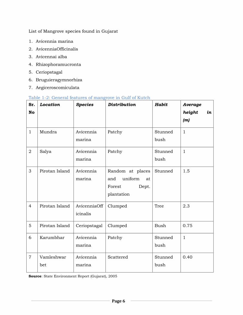
List of Mangrove species found in Gujarat
1. Avicennia marina
2. AvicenniaOfficinalis
3. Avicennai alba
4. Rhizophoramucronta
5. Ceriopstagal
6. Bruguieragymnorhiza
7. Aegiceroscomiculata
Table 1-2: General features of mangrove in Gulf of Kutch
Sr.
No
Location Species Distribution Habit Average
height in
(m)
1 Mundra Avicennia
marina
Patchy Stunned
bush
1
2 Salya Avicennia
marina
Patchy Stunned
bush
1
3 Pirotan Island Avicennia
marina
Random at places
and uniform at
Forest Dept.
plantation
Stunned 1.5
4 Pirotan Island AvicenniaOff
icinalis
Clumped Tree 2.3
5 Pirotan Island Ceriopstagal Clumped Bush 0.75
6 Karumbhar Avicennia
marina
Patchy Stunned
bush
1
7 Vamleshwar
bet
Avicennia
marina
Scattered Stunned
bush
0.40
Source: State Environment Report (Gujarat), 2005

Page 7
The comparative analysis of the previous reports (Forest Department) of year 2001,
2011 and 2014 indicates fluctuation in the mangrove covers for most of the districts.
Majority of the mangrove cover in Gujarat is still located in Gulf of Kutch, witnessing
fluctuation from 706 sq km (2001), 778 sq km (2011) to 672.5 km (2014).For
Jamnagar district, present mangrove cover is estimated at 180.3 sq km in 2014 which
was 142 sq km in 2001, showing an increase. Also, Rajkot district has also shown an
increase in the mangrove cover.
Though, the overall status of mangrove cover across the state has witnessed
fluctuation during 2001-14, the present assessment by BISAG recorded 996.3 sq. km
under mangrove cover which is showing a steep rise to the tune of 88.03 sq. km.
Table 1-3: Change in mangrove cover in Sq km (2001-2014)
District Dense Open Total
2001 2011 2014 2001 2011 2014 2001 2011 2014
Jamnagar 28 28 73.0 114 131 107.0 142 159 180.3
Kutch 118 118 120.4 588 660 552.1 706 778 672.5
Rajkot 0 1 2.7 1 1 6.1 1 2 8.8
Source: FSI, 2001& 2011, BISAG, 2014

Page 8
2 Assignment brief
This study aims to identify the impacts of port-led coal activities on mangroves and its
ecosystem. Though Environment Impact Assessment (EIA) has been carried out before
implementation of port development and expansion activities for all the five selected
sites, this study takes a deeper review on mangroves and marine ecosystems in
context of post development activities with explicit focus on coal handing activities.
Increasing coal demand in Gujarat state has resulted in growing capacity of coal
handling at ports. Activities associated with coal handling, transporting and storage
facilities near the coast increase the possibility of environmental contamination and
requires impact assessments on mangrove ecology & environment. Coal storage and
loading facilities at ports are also potential sites of contamination, often of a very large
scale. Though many coal-handling ports operate best-management practices to reduce
the fugitive losses, such efforts might not be considered adequate if exposure to coal
had noticeably adverse toxic effects on aquatic organisms.
Port areas considered under this assignment are leading ports of Gujarat in terms of
coal export. Since, all five ports are surrounded by mangrove vegetation; coal dust
may pose considerable threat on mangroves which would lead to extensive impact on
overall mangrove ecosystem. Thus, present study focuses on coal handling and its
related impact on mangrove ecosystem. Following are the objectives of the study;
2.1 Aim and objective of the study
Assess the impact of un-burnt coal handing on mangroves within ports of
Gujarat.
Assessment of physicochemical parameter, bio-physical parameter, and heavy
metal impact to ascertain the ecological and environmental status of selected
area.
Identify direct and indirect effects of coal handling on mangroves and related
ecological aspects.
To study the possible ways to minimize and contain the impacts in future.

Page 9
2.2 Scope of study
Present study aims to comprehend the impact of coal dust on mangroves and its
ecology. Probabilities of contamination through leaching and particularly during
loading, transporting, unloading and storage of coal is being considered under this
study. Study focuses on assessment of physicochemical parameter, bio-physical
parameter and soil profiling to ascertain the ecological and environmental status of the
selected area. It also includes physical, chemical, direct and indirect effects of coal
handling on mangroves and related ecological aspects. The residual effect of coal
combustion such as fly ash, by-products of coking and coal gasification are not
considered in this study.
2.3 Limitation of the study
To get a first-hand understanding of factors critical in such type of study, we have
enlisted the limitations faced during the study period.
Time-frame: Due to limited time-frame from client, present study was
contained to 2 months (November-December 2015), thus the mangrove
sampling was not done for all seasons. It is required to observe the flowering
and regeneration pattern of mangroves for one full year (encompassing all 3
seasons) and also the changes in water quality & soil health.
Impacts: Due to limited time-frame, the data presented in this study is specific
to a time-period and the impacts on mangrove observed are only during one
season.
Mangrove Anatomy: The mangroves’ anatomy is affected by both natural as
well as anthropogenic changes. Though this study has focused to understand
the impacts of man-made changes on mangrove ecology (primarily coal dust
and coal handling on ports); other factors such as land-use change, pollution,
shipping, seasonal variation, water quality, soil health, climate change, sea-
level rise, cyclone-tsunami etc. are needed to be studied fully in order to distinct
the magnitude of coal handling activity’s impacts on mangroves.
Legal permission and changing land use: It was observed that the legal
permission from port authorities and concerned government bodies present at
port took lot of time for approval and many times sampling process was delayed
due to that. In one particular case, sampling permission from Mundra port

Page 10
authority and custom department present at Mundra was not given thus
Mundra was excluded from the study. Moreover, coal handling segment of
Mundra port has been sifted to new location (during 2014-15), where mangrove
vegetation was not traced. Hence, Mundra Port assessment was not considered
for impact evaluation.
2.4 Time frame
Deliverables Aug. Sep. Oct. Nov. Dec. Jan.
Desk review and Assessment of Secondary
data, literature.
Development of detail methodology for
impact assessment on mangroves.
Collection of Primary data.
Mapping and detail qualitative and
quantitative assessment of primary and
secondary.
Submission of Draft Report.
Submission of Final Report.

Page 11
3 Study Framework
Limited research work has been conducted on the subject of coal dusts’ impact on
mangrove. Hence, primary step was to frame detailed methodology to carry out
comprehensive research. Review of literature and secondary data assessment was
carried out to structure methodology. Furthermore, respective indicators and sample
locations were identified to support impact evaluation. Indicators were assessed based
on primary survey, containing baseline information. Following chart indicates broad
study framework and detailed methodology:
Figure 3-1: Study Framework

Page 12
4 Methodology and assessment Approach
The approach of the study is designed to identify the stress elements on mangroves
and its ecosystem. There are various factors that interact with an ecosystem likewise
various factors, playing crucial role in the sustenance of mangrove ecosystems.
Coal dust contamination through water, soil and air will hamper mangrove’s health in
direct or indirect manner. Mangroves leaves will come in direct contact with coal dust
through air contamination, whereas air, soil and water contamination would cause
damages through numetophores.
First segment of study covers secondary data and literature review. Trend analysis for
environment pollution, mangrove vegetation change and setting up assessment
indicators were the prime objectives of this segment.
Second segment of the study has determined parameters like physicochemical, heavy
metal in soil and water. The aim behind it was to understand level of polluting agents
in soil and water with specific focus on coal dust pollutants.
Third segment is focused on bio-physical parameter assessment of mangroves. This
has reinforced the evidence of direct impact of coal on mangroves. Assessment was
also supported by coal dust load on leaves and mangrove density.
Baseline data was collected through primary surveys, and comparative assessment
was carried out with respect to controlled site situation. Respective site conditions are
raked according to their exposure to coal impact and extended vulnerability.
Primary data was mapped and evaluated using Geographical Information System (GIS)
technique. Furthermore, multi-dimensional vulnerability has been identified and
quantified. Following image exhibits detail methodological approach, for this study.

Page 13
Figure 4-1: Assessment Approach

Page 14
5 Study Area
The mangrove ecosystem found at
Gulf of Kutch is a very sensitive and
is under stress due to increasing
anthropogenic activities like
industrial developments, waste
disposals, salt rearing, ports and
harbors. In the interior part of Gulf
of Kutch, we can find major ports
which are India’s most import points
for international trade. The project
area has 5 different ports, located at
various geographical locations and
districts. List of the port is given below;
1. Kandla Port, located in Kutch district
2. Navlakhi Port is located in Rajkot district
3. Bedi Port located in Jamnagar district
4. Rozi Port located in Jamnagar district
5. Mundra Port, located in Kutch district
Table 5-1: Details of ports selected for study area
Sr.
No.
Name of
Port
District Ownership Coal Handling
Capacity Per
annum
1 Kandla Port Kutch Government (Major Port) 9.97 MMT
2 Navlakhi
Port
Rajkot Government (GMB minor
Port)
8.05 MTPA
3 Bedi Port Jamnagar Government (GMB minor
Port)
2.5 MTPA
Figure 5-1: Location of ports selected for study area

Page 15
4 Rozi Port Jamnagar Government (GMB minor
Port)
Not applicable (coal
is not handled from
this site.)
5 Mundra
Port
Kutch Private, Owned by Adani
Group
60 MTPA
Source: GMB, 2015
A) Kandla Port
Kandla Port is one of major ports among the 13 declared major ports of India; the port
is located on the shores of Kandla Creek in Kutch district. Presently, Kandla Port
handles cargo at its ten general cargo berths and through barges at Bunder Basin and
Tuna. Both these facilities have a combined capacity of 46.28 Million Metric tonnes
per annum, which includes dry handling capacity of 33.28 MMTPA and liquid cargo
handling capacity of 13.0 MMTPA. Major commodities exchanged at Kandla Port are,
POL and acids, crude oil, edible oil, fertilizers, scrap, steel coils, wooden logs and coal,
Food grains, Salt, Coated/Steel Pipes, Bentonite etc.
2003 2015 Increased area in coal storage %
Kandla port infrastructure development area 1148 Ha 1373 Ha
19%
Kandla coal storage area 41 Ha 137 Ha 234%
Figure 5-2: Kandla port- change in port development during 2003-2015

Page 16
B) Navlakhi Port
Navlakhi Port is located in Rajkot district in Hansthal creek, a non-major intermediate
port governed by Gujarat Maritime Board. Port is handling 10,000 to 15,000 metric
tonnes of cargo per day.
Figure 5-3: Navlakhi port- change in port development during 2003-2015
Major commodities handled at Port of Navlakhi are Coal & Coke, Flourspar, Pig Iron
and exported commodities are Salt.
C) Bedi Port
Bedi port has an annual capacity of handling 6.11 MMT of cargo. Major commodities
handled at Bedi Port are Fertilizer, Rock Phosphate, Coal, Corn, Soya Meal, Crude
Soyabean Oil, Bulgar Wheat, Green Peas, Dates, Refined Vegetable Oil, RBD Palm Oil,
Crude Palm Oil, Rock Salt and Pig Iron, Soyabean ext., Rapeseed ext., Bauxite,
Guargum, Cement, Castor oil, Castor seed, Pet coke, Clinker, Rice, Sugar etc.
2003 2015 Increased
area in %
Navlakhi port
infrastructure
development area
49.3
Ha
59.7
Ha
21%
Navlakhi coal
storage area
33.9
Ha
51.3
Ha
51%

Page 17
2003 2015 Increas
ed area
in %
Bedi port
infrastructure
development
area
6
ha
13.4
ha
123%
Bedi coal
storage area
0
Ha
5.79
Ha
NA
D) Rozi Port
Rozy Port, nestled on shore of Gulf of Kutch, is major port located close to Jamnagar.
Rozy is prominent trading hubs in the Arabian Sea. This port is an extension of Bedi
port, consisting only one jetty and no other infrastructure or storage facility. At
present, it only handles food cargos and shipments. Coal is not being handled from
this port facility currently.
E) Mundra Port
Mundra Port, also known as Adani Port and Special Economic Zone ltd. (APSEZ), is
the largest privately developed port in the country and a multi-sector SEZ. It is spread
over 100 sq. km. in the Northern Gulf of Kutch. APSEZ has a diverse cargo base to
handle various dry, bulk, break bulk, liquid, crude oil, project cargo, cars and
containers. APSEZ has a capacity to handle 100 million tons of cargo annually.
Figure 5-4: Bedi port- change in port development during 2003-2015

Page 18
2003 2015 Increased area in %
Mundra port infrastructure development area 1009 Ha 2046 Ha 102%
Mundra coal storage area 35.5 Ha 77.4 Ha 118%
Figure 5-5: Mundra port- change in port development during 2003-2015

Page 19
6 Literature Review
Impact assessment (IA) simply defined as the process of identifying the future
consequences of current or proposed action. The “impact” is the difference between
what will the scenario with the action taken and what will happen if action not taken.
Impact assessment aims to:
Provide information for decision-making that analyzes the biophysical, social,
economic and institutional consequences of proposed/implemented actions,
Promote transparency and participation of public in decision-making,
Identify procedures and methods for follow-up (monitoring and mitigation of
adverse consequences) in policy, planning and project cycles,
Contribute to environmentally sound and sustainable development.
At international level, Impact Assessment (IA) was fully recognized in 1992 at the
United Nations Conference on Environment and Development, held in Rio de Janeiro.
Principle 17 of the Final Declaration of this summit is dedicated to Environment
Impact Assessment (EIA). Further development and debates on Impact Assessment
has lead the way towards, assessment of other detailed aspects of social, ecology,
health, economy and lifecycle.
These can be carried out independently as well as in a joint exercise with other IA. To
emphasize such integration of different forms of impacts, some professionals and
institutions use the expression Integrated IA. For others, integration of environment,
social and economic dimensions of assessment justify the adoption of a distinct term:
Sustainability Assessment.
Environment Impact Assessment (EIA) and Ecology Impact Assessment
EIA is embedded in legal framework of most countries, and EIA process is carried prior
to implementation of any development project. Ecology and biodiversity is one of the
integral part of EIA assessment, and is given equivalent weightage. There are many
debates, favoring explicate assessment of ecology and biodiversity assessment, since it
is the core as well as the most vulnerable part of environment.
There is a growing awareness of urgent need to modify EIA approaches to explicitly
address the links between EIA and sustainable development (George 1999, Dalal-

Page 20
Clayton 1992). In current regulatory framework, EIA is being carried out in-line with
specific guidelines. These framework and guidelines has certain gaps that can result
in irreversible ecological impacts and unsustainable development. The two aspects
discussed in following segment are the prime step, which can lead EIA towards
sustainability.
A first step for making of EIA, a tool to foster sustainable development, would consist
in adding biodiversity to the list of environmental aspects to be routinely analysed
during the EIA The loss of biodiversity, together with climate change, represents the
main environmental concern addressed by studies in sustainable development
(Diamantini and Zambon 2000). However, covering the topic of biodiversity in EIA is
not mandatory in most legislations, and consequently satisfactory assessments of the
impact on biodiversity are lacking (Atkinson et al. 2000).
The second and most critical aspect deals with assessment of impact. Under
sustainable development, impacts are considered if only they are resilient or adaptive.
The fundamental condition for sustainability consists in keeping the stock of capital
intact, so that future generations are passed on the same amount of capital that exists
now (Pearce et al. 1993). Capital comprises the man-made capital (infrastructures,
houses, etc.), the human capital (knowledge, skills), and the natural capital (soil,
habitat, clean water, etc.). The different types of capital can be freely interchanged
(weak sustainability approach), or alternatively a maximum amount of substitution
between environmental assets and man-made assets can be defined (strong
sustainability approach).
Ecology and Biodiversity Impact Assessment
Ecological evaluation aims at developing and applying methodologies to assess the
relevance of an area for nature conservation. It is meant to support the impact
assessment of a proposed development by providing guidance on describing the
ecological features within the area affected, methods for its valuation, and calculate
the estimated value losses caused by the development. However, limited efforts have
been made in last decade to improve the framework for ecological evaluation, proposed
during 1970s and 1980s, and to adapt them specifically during evolution of EIA
procedures. As a result, assessment of ecological component within EIAs tend to be

Page 21
flawed, and provide conclusions supported by poor evidences and lack clear rationales
(Byron et al. 2000).
The evaluation of ecological significance of an area can be undertaken from different
perspectives, and consequently with different objectives. Amongst such objectives, one
in particular has recently emerged as a key environmental issue: the conservation of
biodiversity. “In little more than a decade, biodiversity has progressed from a short-
hand expression for species diversity into a powerful symbol for richness of life on
earth. Biodiversity is now a major driving force behind efforts to reform land
management and development practices worldwide and to establish a more
harmonious relationship between people and nature” (Noss and Cooperrider 1994).
This quotation best introduces two concepts: Firstly, that biodiversity represents an
actual global concern, more and more addressed by studies aimed at promoting
sustainable development (Pearce et al. 1993, George 1999, and Diamantini, 2000).
And secondly, that biodiversity is itself a relatively recent concept. As a consequence, a
30-years old tool such as EIA does not necessarily include it as an environmental
component to be analysed. Indeed, covering the topic of biodiversity in the EIA is not
mandatory in early EIA legislations, such as that of North America or of Europe. Even
though, in such legislations, biodiversity may be considered somehow implicit in the
analysis of ecological component, its explicit treatment is widely advocated, due to the
complexity and growing relevance of the topic.
Several governmental agencies have issued guidance on EIA and biodiversity
(Canadian Environmental Assessment Agency 1996, CEQ 1993) and work is being
carried out in this area also by a range of non-governmental bodies, such as the
International Association for Impact Assessment (IAIA 2001) and The World
Conservation Union (Byron 1999). This has led to establishment of a specific
disciplinary field, namely Biodiversity Impact Assessment (BIA), which aims at
developing and applying strategies for performing the analysis of the impacts on
biodiversity within EIA.
Sources and distribution of particulate coal in the marine environment
Anthropogenic inputs of coal occur at several stages of the coal utilization. These
include: disposal of colliery waste into intertidal or offshore areas (Limpenny et al.
1992, McManus 1998); wind and water erosion of coastal stockpiles (Zhang et al.

Page 22
1995); coal washing operations (Williams & Harcup 1974); spillage from loading
facilities (Sydor & Stortz 1980, Biggs et al. 1984);‘cargo washing’ (the cleaning of ships’
holds and decks after offloading dry bulk cargoes by washing with water and
discharging over the side;(Reid & Meadows 1999); and the sinking of coal-powered and
coal-transporting vessels (Ferrini & Flood 2001).
As a result of these various inputs, unburnt coal occur very commonly in marine
sediments which may represent a considerable proportion of the sediment. The
abundance of coal in marine environment is likely to be greatest adjacent to storage
and loading facilities in coal producing and importing countries, around spoil grounds
receiving colliery waste, along shipping lanes and in areas receiving terrestrial runoff
from catchments where coal mining occurs (French 1993b, Allen 1987).
Impact of coal on Marine Ecosystems
Prime effect of coal handing on mangrove ecology is physical, such as smothering and
abrasion. Furthermore, chemical composition of coal can have varying effects on
mangroves, depending on coal type and chemical composition. Effects can extent to
mangroves biological levels of the cell, organism and population.
A. Physical effects of coal on marine organisms
Moore (1977) reviewed the effects of particulate, inorganic suspensions on marine
animals and (Airoldi 2003) reviewed the effects of sedimentation on biological
assemblages of rocky shores. Moore (1977) made the distinction, from the perspective
of biological effects, between scouring by larger particles, such as sands, and the
turbidity-creating effects of smaller particles, such as silts and clays. Many animals
and plants living on rocky shores trap sediments and, thereby, influence rates of
sediment transport, deposition and accretion (Airoldi 2003), and this is equally true
for animals living in soft sediment habitats (Norkko et al. 2001).The reviews by Moore
(1977) and Airoldi (2003) show that, conversely, sediments affect the abundance and
composition of marine organisms and assemblages when in suspension and following
deposition.
B. Direct effects of coal
Increased concentrations of suspended particulate coal in water column may cause
abrasion of animals and plants living on the surface of sea bed or on structures such

Page 23
as rocks or wharf piles (Airoldi 2003). The probability and severity of this effect will
depend on concentration, size and angularity of coal particles and on strength of water
currents (Lake & Hinch 1999). Newcombe & MacDonald (1991) pointed out that the
particle dose to which an organism is exposed (a function of the concentration of
suspended material and the duration of exposure) is a more relevant measure of stress
than concentration alone but that duration is often not reported in studies of the
effects of suspended sediments.
Particles of coal in suspension will also reduce the amount and possibly the spectral
quality (Davies-Colley & Smith 2001) of light that reaches the seabed or other
underwater surfaces, in a manner similar to other suspended particles (Moore 1977).
This, in turn, may affect growth of plants such as mangroves, seaweeds, sea grasses,
and microalgae on the surfaces of sediments and rocks (Dennison1999, Moore et al.
1997).
Deposition of coal dust on the surface of plants above and below water may also
reduce photosynthetic performance. Mangroves growing around South Africa’s largest
coal-exporting port, Richards Bay, accumulate deposits of coal dust on both upper
and lower leaf surfaces and on branches and trunks (Naidoo & Chirkoot 2004). The
presence of the dust reduced photosynthesis, measured as carbon dioxide exchange
and chlorophyll fluorescence, by 17–39%. There was no evidence that coal particles
were toxic to the leaves, but mangroves closest to the source of the dust appeared to
be in poorer health than those further away. The amount of dust accumulated on
leaves varied among mangrove species, with Avicennia marina, which has relatively
hairy leaves, accumulating more than Bruguieragymnorr hizaor Rhizophoramucronata.
C. Indirect effects
Indirect physical effects may also be biologically mediated (Chapman 2004).Reduction
in growth and abundance of plants as a result of reduced water clarity with
consequent effects on primary consumers, inhibition of recruitment or removal of
adult competitors, predators or grazers, selection of tolerant species and a host of
other factors may give rise to a range of indirect physical effects of the presence of
suspended and deposited sediment in the marine environment (reviewed by Moore
1977 and Airoldi 2003). Reduced water clarity can also reduce the feeding efficiency of
visual predators such as fishes (Wilber & Clarke 2001).

Page 24
D. Chemical effect of coal on mangroves and marine ecology
From a chemical standpoint, coal is a heterogeneous mixture of carbon and organic
compounds, with a certain amount of inorganic material in the form of moisture and
mineral impurities (Ward1984). In addition to its predominant elemental building
block, carbon, coal contains a multitude of inorganic constituents that may greatly
affect its behavior in, and interactions with, the environment. Unburnt coal can be a
significant source of acidity, salinity, trace metals, hydrocarbons, chemical oxygen
demand and, potentially, macronutrients to aquatic environments, which pose
potential hazards to aquatic organisms (Cheam et al. 2000). Trace metals and
polycyclic aromatic hydrocarbons (PAHs) are present in amounts and combinations
that vary with the type of coal. A fraction of these compounds may be leached from
coal upon contact with water, such as during open storage or after spillage into the
aquatic environment (Figure 6.1).
Figure 6-1: Coal effect in marine environment6
(Source: Michael J. and Donald M. 2005, Biologic effects of unburnt coal in the marine environment, researchgate,
article in oceanography and marine biology, New Zealand.)
Whether these can be leached from the coal matrix and affect aquatic organisms will
depend on the type of coal, its mineral impurities and environmental conditions,

Page 25
which together determine how desirable these potential contaminants are? For
example, leaching of metals and acids strongly depends on coal composition, particle
size and storage conditions and is accelerated in presence of oxygen or oxidising
agents and if coal remains wet between leaching events (Davis & Boegly 1981a,b,
Querol et al. 1996).

Page 26
7 Secondary Data assessment
Following table is comprehensive list of secondary data, which were collected and
assessed. It also cites sources of relevant data.
List of secondary data
Sr.
No
Data Type Details Sources
1 Coal
Handling
Coal requirement, import and
export
Coal handling capacity at port and
coal handling process
Coal dust production and
dispersion
Chemical properties of coal dust
and impacts of coal dust on marine
ecosystems
Impacts of coal dust on mangrove
and mangrove ecosystems
Annual reports of
GPCB
Annual reports of
APSEZ
Publications by Kandla
Port Trust
Gujarat Maritime
Board reports
Research Papers
2 Mangroves List of mangroves species found in
Gujarat and classification of
mangroves
Status of mangrove in Gujarat and
district wise mangrove cover
Status report by Forest
Survey of India
Annual reports by
Gujarat Biodiversity
Board
Atlas by BISAG
3 Water Physicochemical data for sea water
at various port and harbor region
in Gulf of Kutch
Heavy metal found in the sea water
in Gulf of Kutch
Standard for water quality in
marine environment as per the
Standards by CPCB
and GPCB
Research papers and
Journals (specify the
papers)
EIA reports
Annual reports of

Page 27
norms of CPCB and GPCB GPCB
4 Soil Texture and chemical composition
of soil at the coastal regions
Heavy metals contamination in
coastal soil of Gulf of Kutch
Impact of coal dust on the soil and
soil health
EIA reports of various
ports
Research Papers and
Journals (specify the
papers)
Following segment of the report exhibits secondary data analysis for water and soil.
Depending on the availability of secondary data, water parameters for Kandla,
Mundra, Navlakhi, and Rozi was compiled and analyzed. Soil parameters were
analyzed for Kandla and Mundra1. The secondary data was assessment for years 2010
to 2013.
7.1 Sea water quality
A) pH values for sea water
Source: Monitoring report- Gulf of Kutch, GPCB (2013)
pH values are used to estimate the acidity/alkalinity of water samples. For all the
major sites ph values falls under norms specified by Central Pollution Control Board
(CPCB standards provided in Annexure II). The ph values for all these sites are within
the permissible limit of 7 to 8.15. Maximum ph is observed at port of Navlakhi and
1 Water parameter Bedi port and soil parameters for Bedi, Rozi and Mundra were not incorporate in this segment, since
consistent data for 2011 to 2014 was not available.
8.16
7.897.63 7.66
7.857.65
8.12 8.14
7
7.5
8
8.5
9
2010 - 2011 2012/2013 2010 - 2011 2012/2013 2010 - 2011 2012/2013 2010 - 2011 2012/2013
Navlakhi Mundra Kandla Rozi
pH values for sea water
pH values for sea water Permisable limit as per the norms of CPCB for pH

Page 28
Rozi 8.16 and 8.15 respectively. Variations were observed in the yearly readings for
Navlakhi where pH drops from 8.16 in 2010-2011 to 7.89 in 2011-2012. All other sites
showed no significant variation year wise.
B) Biological Oxygen Demand (BOD)
Source: Monitoring report- Gulf of Kutch, GPCB (2013)
BOD represents the required dissolved oxygen content required by the organic life
form in the water body to break down the organic matters. Variations regarding the
availability of BOD are observed in data collected. The BOD levels for Navlakhi and
Rozi port are within permissible limits, while Mundra and Kandla port have shown
high levels of BOD, with 27 mg/l and 21.89 mg/l respectively, which is too high for
permissible limits (CPCB standards provided in Annexure II). Mundra and Kandla
shows significant rise in BOD during 2012-13.
C) Chemical Oxygen Demand (COD)
Source: Monitoring report- Gulf of Kutch, GPCB (2013)
25
9.52
27
11.8
21.89
2.585
2010 - 2011 2012/2013 2010 - 2011 2012/2013 2010 - 2011 2012/2013 2010 - 2011 2012/2013
Navlakhi Mundra Kandla Rozi
BOD value for sea water in mg/l
BOD values for sea water Standard for BOD as set by CPCB
51.2 56 38
92.6556.57 74.8
2010 - 2011 2012/2013 2010 - 2011 2012/2013 2010 - 2011 2012/2013
Navlakhi Mundra Kandla
COD values for sea water in mg/l
COD value for sea water Permisable limit as per the norms of CPCB

Page 29
Chemical Oxygen Demand quantifies the amount of oxygen consumed per unit of
water; hence it gives an indirect account of the organic matter found in water. It is
mostly used for the quality assessment of water. COD values for all ports are within
norms of CPCB which is below 250 mg/l. Maximum level of COD is found at Mundra
port which is 92.65 mg/l. The level of COD in sea water for Mundra port shows
variation temporally. For the year of 2010-2011 the COD level is lowest for all ports
and for year 2012-2013, level of COD is maximum for all port with 92.65 mg/l
concentration.
D) Dissolved Oxygen (DO)
Source: Monitoring report- Gulf of Kutch, GPCB (2013)
E) Suspended Solids
Source: Monitoring report- Gulf of Kutch, GPCB (2013)
5.95 6
4.8 4.92 5.25.65 5.5 5.39
2010 - 2011 2012/2013 2010 - 2011 2012/2013 2010 - 2011 2012/2013 2010 - 2011 2012/2013
Navlakhi Mundra Kandla Rozi
DO values for sea water in mg/l
DO for sea water Permisable limits set as per the norms of CPCB
321
777
56162 170 190
26.5 26.9
2010 - 2011 2012/2013 2010 - 2011 2012/2013 2010 - 2011 2012/2013 2010 - 2011 2012/2013
Navlakhi Mundra Kandla Rozi
Suspended solids for sea water in mg/l
Suspended solids found in sea water Permisable limit for suspended solid as per CPCB norms

Page 30
Suspended solids are the particles found in water in form of colloids. The
concentration of suspended particles at Navlakhi exceeds the permissible limits set by
the norms of CPCB. Navlakhi port has the maximum suspended particles’
concentration with 777 mg/l while Rozi has the least at 26.5 mg/l which is within
permissible limits. Mundra and Kandla also exceed the permissible limit of suspended
particles but have very less concentration as compared to Navlakhi. Navlakhi and
Mundra have shown a significant rise in the concentration between year 2010 to 2013.
F) Chlorides
Source: Monitoring report- Gulf of Kutch, GPCB (2013)
The concentration of chlorides is found to be exceeding the permissible limit highly for
all sites. Mundra has the highest concentration of chlorides in seawater with 25601
mg/l concentration in 2010-2011. Navlakhi has the lowest of concentration of all the
given sites but still the concentration of chlorides, which is still above the permissible
levels, with 17873 mg/l in 2010-2011 and 17581 in 2012-2013. There is not much
significant variation observed temporally for the given sites but little reduction in
concentration compared to previous year’s data.
17873 17581
25601 25153 25351 23978 22475 22326
2010 - 2011 2012/2013 2010 - 2011 2012/2013 2010 - 2011 2012/2013 2010 - 2011 2012/2013
Navlakhi Mundra Kandla Rozi
Chlorides concentraion for sea water in mg/l
Chlorine concentration in sea water Permissible limit as per the norms of CPCB

Page 31
G) Sulphates
Source: Monitoring report- Gulf of Kutch, GPCB (2013)
Sulphates are the ions formed of SO42- found in water. The concentration of sulphates
varies for studied sites. The concentration is significantly high for most sites except
couple of cases where it appears within permissible levels. Maximum concentration of
sulphates is recorded at Kandla during 2010-2011 compared to all other ports. The
minimum concentration of sulphates is found at Mundra for in 2012-2013, which is
within permissible limits at 559.67 mg/l.
H) Phosphate
Source: Monitoring report- Gulf of Kutch, GPCB (2013)
Phosphates are inorganic salts of PO43-phosphoric acid; the concentration of
phosphates is relatively low and within permissible levels for all sites. Maximum
concentration of phosphate particles is found in Mundra at 0.693 mg/l compared to
2144
1576
2036
559.67
2272
603
1207
1724
2010 - 2011 2012/2013 2010 - 2011 2012/2013 2010 - 2011 2012/2013 2010 - 2011 2012/2013
Navlakhi Mundra Kandla Rozi
Sulphate conten for sea water in mg/l
Sulphate content in sea water Permissible limit for sulphate as per the norms of GPCB
0.0160.33
0.693
0.0560.33
0.116 0.034 0.0520
0.5
1
1.5
2
2.5
3
3.5
2010 - 2011 2012/2013 2010 - 2011 2012/2013 2010 - 2011 2012/2013 2010 - 2011 2012/2013
Navlakhi Mundra Kandla Rozi
Phosphate content in sea water in mg/l
Phosphate content in sea water Permissible limits for phosphate as per the norms of GPCB

Page 32
other sites. Minimum value of phosphate concentration in sea water is found in
Navlakhi at 0.016 mg/l and at Rozi with concentration of 0.034 mg/l. Navlakhi shows
increase in concentration of phosphate in 2012-2013 with 0.33 mg/l whereas Mundra
and Kandla shows decrease in concentration of phosphate in 2012-2013 with
concentration of phosphate at 0.056 mg/l and 0.116 mg/l respectively.
I) Nitrate
Source: Monitoring report- Gulf of Kutch, GPCB (2013)
Concentration of nitrates for all sites is found within permissible levels. Kandla port
has the maximum concentration of nitrates at 2.215 mg/l followed by Mundra at
1.154 mg/l. Compared to this, the concentration on other sites are relatively lower
with maximum concentration of nitrate in Navlakhi at 0.619 mg/l. Mundra showed a
slight increase in concentration of nitrate in 2012-2013 from 2010-2011 which was at
0.313 mg/l, while Kandla shows a decrease in concentration of nitrate in 2012-2013
compared to 2010-2011 with concentration reducing to 1.04 mg/l.
J) Heavy metals in water
Port Heavy Metals Details Year
Mundra Boron, Selenium,
Chromium
As per the source, no content of heavy
metal was found.
2006
Navlakhi Iron, Lead,
Manganese,
Trace amount of Fe was found in the
marine waters around Navlakhi,
2011
0.29 0.619 0.313 1.154 2.215 1.04 0.062 0.190
5
10
15
20
25
2010 - 2011 2012/2013 2010 - 2011 2012/2013 2010 - 2011 2012/2013 2010 - 2011 2012/2013
Navlakhi Mundra Kandla Rozi
Nitrate content in sea water in mg/l
Nitrate content found in sea water Permissible limit for nitrate in mg/l

Page 33
Chromium concentration of Fe was 0.003 mg/l.
Concentration of Pb, Mn and Cr were
found to be below detection level.
The concentration of heavy metals
where found within permissible limits
as per the norms of CPCB.
Kandla Mercury
Cadmium
Trace amount of Cd, Pb and M were
found in seawater sample.
The concentration of Cd, Pb and M
where quantified at <0.02 mg/l, <0.01
mg/l, <0.005 mg/l respectively.
The concentration of heavy metals
where found within permissible limits
as per the norms of CPCB.
2013
In secondary data analysis, heavy metal contamination was found to be falling within
permissible limits (as per CPCB’s guidelines) for all studied port sites.
7.2 Soil quality
This segment gives details about the chemical property, texture and composition of
soil around port region based upon secondary data collection. As per the data
collected, soil found around Kandla port is sandy loam which indicates a significant
content of silt along with sand in its composition. The soil around Kandla port is
composed of 18-20% silt particles and 72-76% of sandy particles.
K) Texture and composition of soil around Kandla Port
Location Texture Sand % Silt % Clay
Kandla creek Sandy Loam 72 20 8
Jetty Sandy Loam 76 18 6
Source: Monitoring report- Gulf of Kutch, GPCB (2013)

Page 34
From the data, it can be interpreted that the pH of soil is neutral to basic. The
electrical conductivity of soil around jetty region is more compared to soil around
creek region. Chemical content around jetty area is also higher compared to soil found
in creek region. The average concentration of N, P, K ranges between 7.51 to 14.4
mg/100g, 46.2 to 65.21 mg/100g and 24 to 40 mg/l respectively.
A) Chemical properties of soil around Kandla port
Parameters Kandla creek Jetty
pH 7.12 7.32
Conductivity µmhos/cm 5510 7310
N (mg/100g) 7.51 14.4
P (mg/100g) 46.2 65.21
K (mg/100g) 24 40
Mg (mg/100g) 5.58 4.45
Suplhate 3.1 3.28
Chloride 30.14 34.5
Sodium 15.45 20.1
Source: Monitoring report- Gulf of Kutch, GPCB (2013)
B) Texture and composition of soil around Navlakhi port
Soil around Navlakhi port is sandy soil, which suggests high percentage of sand
particles in soil. Sand particles consist 74 to 80% of soil while rest is silt and clay.
Location Texture Sand % Silt % Clay
GMB Jetty Sandy 80.5 8.5 6
New Navlakhi Sandy 74 8 7
Source: Monitoring report- Gulf of Kutch, GPCB (2013)

Page 35
pH of soil varies from 7.04 to 7.80 which indicates that soil is neutral to basic in
nature. The chemical composition of soil near jetty area has more concentration of
chemical constituent compared to overall region. The basic nutrient N, P, K, necessary
for the estimation of soil quality, ranges between 1.5 to 2 mg/100g, 0.9 to 3.5
mg/100kg and around 1.2 respectively. Organic content is the most important aspect
of soil health and the organic matter content in soil is around 1.1%.
C) Chemical Parameters of soil around Navlakhi port
Parameters GMB jetty Navlakhi
pH 7.81 7.04
Mg 2.5 0.8
Sodium 5.2 4.5
Phosphate 3.5 0.9
Potassium 1.2 1
N 2 1.5
Organic matter % 1.1 1.2
Source: Monitoring report- Gulf of Kutch , GPCB (2013 )
D) Heavy metals in soil
Port Heavy Metals Details Year
Navlakhi Iron, Copper,
Manganese, Zinc
Fe was quantified at 29.1 mg/100g and
Cu was quantified to be 1.5 mg/l from
soil samples around Navlakhi.
The amount of Mn and Zn where found
to be below detection level.
2011
Kandla Cadmium, Lead and
manganese
Trace amount of Cd, Pb and M were
found in seawater sample.
2013

Page 36
The concentration of Cd, Pb and M
where quantified at <0.02 mg/Kg, 1.25
mg/Kg, <0.005 mg/Kg respectively
Source: Monitoring report- Gulf of Kutch, GPCB (2013)
Heavy metal contamination in soil at Kandla and Navlakhi found below detection level
and within permissible limit of CPCB.

Page 37
8 Primary data collection
This segment of the project solely focuses on ground truthing and data collection for
quantitative assessment. To assess the impacts of coal dust, major focus has been laid
on primary data and ground level assessment.
Five sites (four ports and one pristine site) have been included under primary data
collection segment. Number of samples and locations has been chosen based on GIS
map and port locations. Further segment of the report includes sample location and
strategies adopted for the same.
8.1 Adapted sampling strategy
Figure 8-1: Kandla port- sample location
Figure 8-2: Navalhi port-sample location
Figure 8-3: Bedi port-sample location
Figure 8-4: Rozi port-sample location
Before starting sample collection, we have ensured that collected samples will
represent aqueous system. In order to collect the representative and homogenous
samples, site assessment has been done though GIS mapping. Three buffer areas of 1
KM, 2 KM, and 3 KM were mapped putting center in port locations. Samples have
been collected from each of buffer areas, to understand spatial effect of coal dust on

Page 38
surrounding areas. Following images represents location of sample collection and
mapped buffer areas.
Following table contains details of sample locations covered under primary survey.
Further details of locations along with GPS locations have provided in Annexure I.
Table 8-1: Primary table
Type of assessment Number of sample
location
Water Physicochemical parameter assessment
Heavy metal contamination assessment
6
Soil Physicochemical parameter assessment
Heavy metal contamination assessment
12
Mangrove
health
Anatomical Assessment Pigment Analysis
Dust Load Carbon Content estimation Leaf
moisture content Morphological Assessment
Heavy Metal Assessment
16
Figure 8-5: Collection of soil samples

Page 39
8.2 Lab Testing Methods
Water and soil samples collected during primary survey have been sent for testing at
an ISO-9001certified Gujarat laboratory. Laboratory results of samples investigated
are provided in Annexure III. Detailed parameters considered for laboratory testing
and methodology is given in following segment.
8.2.1 Physiochemical parameters for water
pH at 25 Dec C
Total Dissolved solid
Mg/1
Colour
Turbidity
Total hardness
Biological oxygen demand
Chemical oxygen demand
Total suspended solid
Electric conductivity
Fluoride
Phosphate
Nitrate
Sulphate
8.2.2 Laboratory Methods to assess physiochemical parameters
pH
I. Apparatus
a) pH meter with temperature compensating device, accurate and reproducible to
0.1 pH unit with a range of 0 to 14.
b) Reference electrode preferably with quartz liquid junction. Follow
manufacturer’s instructions on use and care of the reference electrode. Refill
non-sealed electrodes with correct electrolyte to proper level and make sure
junction are properly wetted.
c) Glass electrode. Follow manufacturer’s instructions on use and care of
electrode.
II. Reagents
a) Potassium hydrogen phthalate buffer, 0.05m, pH 4.00. Dissolve 10.12 g
KHC8H4O4 (potassium hydrogen phthalate) in 1000ml freshly boiled and cooled
distilled water.
b) 0.025M Potassium dihydrogen phosphate + 0.025m disodium hydrogen
phosphate buffer, pH 6.86. Dissolve 3.387 g KH2PO4 + 3.533 g Na2HPO4 in
1000ml freshly boiled and cooled distilled water.

Page 40
c) 0.01M sodium borate decahydrate (borax buffer), pH 9.18. Dissolve 3.80 g
Na2B4O7.10H2O in 1000ml freshly boiled and cooled distilled water.
d) Store buffer solutions in polyethylene bottles. Replace buffer solutions every 4
weeks.
III. Procedure
a) Remove electrodes from storage solution, rinse, blot dry with soft tissue, placed
it in initial buffer solution and standardise pH meter according to
manufacturer’s instructions.
b) Remove electrodes from first buffer, rinsed thoroughly with distilled water, blot
dry and immerse in second buffer preferably of pH within 2 pH units of the pH
of the sample. Read pH, which should be within 0.1 unit of the pH of the
second buffer.
c) Determined pH of the sample using the same procedure as in (b) after
establishing equilibrium between electrodes and sample. For buffered samples
this can be done by dipping the electrode into a portion of sample for 1 min.
Blot dry, immerse in a fresh portion of the same sample, and read pH.
d) With dilute poorly buffered solutions, equilibrate electrodes by immersing in
three or four successive portions of the sample. Take a fresh sample to measure
pH.
e) Stir the sample gently while measuring pH to insure homogeneity.
Total Dissolved Solids
I. Apparatus
a) Evaporating dishes, 100 ml capacity of porcelain, platinum or high-silica glass
made
b) Drying oven, 104 ± 1°C
c) Desiccator
d) Magnetic stirrer
e) Glass-fibre filter disk, Whatman grade 934 AH, Gelman type A/E, Millipore type
AP4O or equivalent, diameter 2.2 to 12.5 cm.
f) Filtration apparatus, Membrane filter funnel or Gooch crucible with adapter
and suction flask of sufficient capacity for sample size selected
II. Procedure

Page 41
a) Washed filter paper by inserting it in the filtration assembly and filtering 3
successive 20 mL portions of distilled water. Continued suction to remove all
traces of water. Discarded washings.
b) Dry evaporated dish at 104 ± 10C for 1 h, cool and store in desiccator. Weighed
immediately before use.
c) Stirred sample with a magnetic stirrer and while stirring pipette a measured
volume on to the filter using a wide bore pipette. Choose sample volume to yield
between 10 and 200 mg dried residue. Wash with three successive 10 mL
volumes of distilled water. Continuous suction for about 3 min after filtration
completed.
d) Transfer the total filtrate with washings to a weighed evaporating dish and
evaporate to dryness in an oven at 104 ± 10C. If necessary, added successive
portions to the same dish after evaporation in order to yield between 10 and
200 mg dried residue. To prevent splattering oven temperature may be lowered
initially by 2 0C below boiling point and raised to 104 0 C after evaporation for
1h. Cool in a desiccator and weigh.
III. Calculation
Dissolved Solids mg /L = (A− B) ×1000 / ml sample
where:
A = weight of dried residue + dish, mg
B = weight of dish, mg.
Turbidity
I. Apparatus
a) Nephelometric turbidity meter with sample cells
II. Reagents
a) Solution I. Dissolve 1.000g hydrazinesulphate, (NH2) 2.H2SO4 in distilled water
and dilute to 100ml in a volumetric flask.
b) Solution II. Dissolve 10.00g hexamethylenetetramine, (CH2) 6N4, in distilled
water and dilute to 100ml in a volumetric flask.

Page 42
c) 4000 NTU suspension. In a flask mix 5.0ml of Solution I and 5.0ml of Solution
II. Let stand for 24 h at 25 ± 3°C. This results in a 4000 NTU suspension. Store
in an amber glass bottle. The suspension is stable for up to 1 year.
d) Dilute 4000 NTU stock solution with distilled water to prepare dilute standards
just before use and discard after use.
III. Procedure
a) Calibrate nephelometer according to manufacturer’s operating instructions.
Run at least one standard in each instrument range to be used.
b) Gently agitated sample. Waited until air bubbles disappear and pour sample
into cell. Read turbidity directly from instrument display.
Total Hardness
I. Reagents
a) Buffer solution: Dissolve 16.9g NH4Cl in 143 mL conc. NH4OH. Added 1.25g
magnesium salt of ethylenediaminetetraacetate (EDTA) and dilute 250 ml of
distilled water. Store in a plastic bottle stoppered tightly for no longer than one
month.
b) Complexing agent: Magnesium salt of 1, 2 cyclohexanediaminetetraacetic acid.
Added
c) 250mg per 100 ml sample only if interfering ions are present and sharp end
point is not obtained.
d) c. Indicator: Eriochrome Black T sodium salt. Dissolve 0.5g dye in 100 ml
triethanolamine or 2 ethylene glycol monomethyl ether. The salt can also be
used in dry powder form by grinding 0.5g dye with 100g NaCl.
e) d. Standard EDTA titrant, 0.01m: Weigh 3.723g di-sodium salt of EDTA,
dihydrate, dissolved in distilled water and dilute to 1000 ml. Stored in
polyethylene bottle.
f) e. Standard Calcium Solution: Weigh 1.000g anhydrous CaCO3 in a 500 ml
flask. Added HCl slowly through a funnel till all CaCO3 is dissolved. Added 200
ml distilled water and boil for a few minutes to expel CO2. Cool and add a few
drops of methyl red indicator and adjust to the intermediate orange colour by
adding 3N NH4OH orHCl, as required. Transfer quantitatively and dilute to
1000 ml with distilled water, 1 ml = 1mg CaCO3.
II. Procedure

Page 43
a) Dilute 25ml sample to 50ml with distilled water. Added 1 to 2ml buffer to give a
pH of10.0 to 10.1. Added 1 to 2 drops of indicator solution and titrate with
EDTA titrant to changeitscolour from reddish tinge to blue. Select a sample
volume that requires less than 15mlEDTA titrant and completed titration within
5 min after buffer addition.
b) Standardise the EDTA titrant against standard calcium solution used in above
procedure.
III. Calculation
Total Hardness (EDTA),mg CaCO3 /L= A ×B ×1000 ml sample
Where:
A = mL EDTA titrated for sample
B = mg CaCO3 equivalent to 1.00 mL EDTA titrant
Biochemical Oxygen Demand
I. Apparatus
a) BOD bottles, 300 mL, narrow mouth, flared lip, with tapered and pointed
ground glass stoppers.
b) Air incubator or water bath, thermostatically controlled at 27 ± 1°C. Light entry
must be prevented in order to avoid photosynthetic oxygen production
c) Accessories: plastic tube, screw-pin and a 5-10 L water container.
II. Reagents
a) Phosphate buffer solution. Dissolved 8.5 g KH2PO4, 21.75 g K2HPO4, 33.4 g
Na2HPO4.7H2O and 1.7 g NH4Cl in 1L distilled water.
b) Magnesium sulphate solution. Dissolved 22.5 g MgSO4.7H2O in 1L distilled
water.
c) Calcium chloride solution. Dissolved 27.5 g CaCl2 in 1L distilled water.
d) Ferric chloride solution. Dissolved 0.25 g FeCl3.6H2O in 1L distilled water.
e) Acid and alkali solution. 1N NaOH and 1N H2SO4. Used for neutralising
samples.
f) Glucose-glutamic acid solution (prepare fresh). Dissolve 150 mg dry reagent
grade glucose and 150 mg dry reagent grade glutamic acid in 1L distilled water

Page 44
g) Sample dilution water. Add 1 mL each of phosphate buffer, MgSO4, CaCl2 and
FeCl3 solutions per liter distilled water.
III. Procedure
a) Prepare required amount of dilution water at the rate of 1000 to 1200 mL per
sample per dilution. Bring the diluted water temperature to 27°C. Saturate with
air by shaking in a partially filled bottle, by bubbling with organic free filtered
air or by storing in cotton plugged bottles for a day.
b) Some samples do not contain sufficient microbial population (for example, some
industrial wastes, high temperature wastes, or wastes with extreme pH values).
For such wastes, the dilution water is seeded using effluent from a biological
treatment system processing the waste. Where this is not available, use
supernatant from domestic wastewater after settling for at least 1 h but not
more than 36 h. Seed from a surface water body receiving the waste may also
be suitable. Add enough seed volume such that the DO uptake of the seeded
dilution water is between 0.6 and 1.0 mg/L. For domestic wastewater seed,
usually 4 to 6 mL seed / L of dilution water is required. Surface water samples
usually do not require seeding.
c) Dilution of sample. Dilutions must result in a sample with a residual DO (after
3 days of incubation) of at least 1 mg/L and a DO uptake of at least 2 mg/L.
Make several dilutions using the Table and experience with the particular
sample source. Polluted surface waters may have 5 to 25 mg/L BOD.
d) For preparing dilution in graduated cylinders, siphon dilution water, seeded if
necessary, into a 1 to 2 L capacity cylinder. Siphoning should always be done
slowly without bubbling, use a screw-pin on the tube to regulate the flow. Keep
the tip of the tube just below the water surface as it rises. Fill cylinder half full,
add desired quantity of sample and dilute to appropriate level, mix with plunger
type mixing rod. Siphon mixed diluted sample.
e) BOD bottles, stopper without entraining any air. Determine initial DO (method
1.9) on one bottle and incubate the other two at 27°C. Determine final DO in
duplicate after 3days.
f) For direct pipetting, siphon the desired sample volume to individual bottles and
fill with enough dilution water. Complete the test as in the earlier case.

Page 45
g) Dilution water blank. Find the DO consumption of unseeded dilution water by
determining initial and final DO as in c above. It should not be more than 0.2
mg/L
h) Seed control. Determine the DO uptake by seeding material according to the
procedure in c above.
IV. Calculation
When dilution water is not seeded : BOD mg/L= DO- DT / P
When dilution water is seeded BOD mg/L= (D0 - DT) – f × (BO - BT ) / P
where:
D0 = DO of diluted sample initially, mg/L
DT = DO of diluted sample after 3 day incubation at 27°C, mg/L
P = decimal volumetric fraction of sample used, L
B0 = DO of seed control initially, mg/L
BT = DO of seed control after incubation, mg/L
f = ratio of %seed in diluted sample to %seed in seed control
Dissolved Oxygen
I. Apparatus
a) DO sampler, for collection of undisturbed samples from surface waters.
b) BOD bottles, 300 mL, narrow mouth, flared lip, with tapered and pointed
ground glass stoppers.
c) One siphon tube.
II. Reagents
a) Manganoussulphate solution. Dissolve 480 g MnSO4 .4H2O, 400 g MnSO4.2H2O
or 364 g MnSO4.H2O in distilled water, filter and dilute to IL.
b) Alkali-iodide-azide reagent. Dissolve 500 g NaOH (or 700 g KOH) and 135 g NaI
(or 150g KI) in distilled water and dilute to IL. Added 10 g NaN3 dissolved in 40
mL distilled water.
c) conc. Sulphuric acid

Page 46
d) Starch indicator. Dissolve 2 g laboratory grade soluble starch and 0.2 g salicylic
acid as a preservative, in 100 mL hot distilled water.
e) Standard sodium thiosulphate titrant, 0.025M. Dissolve 6.205 g Na2S2O3.5H2O
in distilled water. Add 1.5 mL 6NNaOH or 0.4 g solid NaOH and dilute to 1000
mL. Standardize with bi-iodate solution.
f) Standard potassium bi-iodate solution, 0.0021M, Dissolve 812.4 mg KH(I03)2 in
distilled water and dilute to 1000 mL .
g) Standardization: Take 100 to 150 mL distilled water in an Erlenmeyer flask.
Add approximately 2g KI, dissolve. Add 1 mL 6N H2S04 or a few drops of conc.
H2SO4 and 20 mL bi-iodate solution. Dilute to 200 mL and titrate liberated
iodine with thiosulphate titrant to a pale straw colour. Add a few drops of
starch indicator. Continue titration to first disappearance of blue colour.
Calculate molarity, M of thiosulphate as:
M = 20*0.0126 / V
where:
V = mL of thiosulphate used
III. Procedure
a) Drain any liquid in the flared lip of the BOD bottle containing the sample.
b) Removed stopper and add 1 mL of MnSO4 followed by 1 mL alkali-iodide-azide
reagent. Hold the pipette tip just below the liquid surface touching the side of
the bottle. Wash the pipette before returning to the reagent bottles.
c) Stopper carefully to exclude air bubbles. Mix by inverting the bottle a few times.
d) Allow the brown manganese hydroxide floc (white floc indicates absence of DO)
to settle approximately to half the bottle volume, add 1.0 mL conc. H2SO4 and
re-stopper. Mix by inverting several times until dissolution is complete.
e) Titrate 201 mL with standard Na2S2O3 as for standardization procedure
described above.
IV. Calculation
DOmg/L= V x M/ 0.025
where:

Page 47
V = mL thiosulphate solution used
M = molarity of thiosulphate titrant
Sodium
I. Apparatus
a) Flame photometer, direct reading type.
b) Glassware, rinse with 1 + 15 HNO3, followed by de-ionized distilled water.
c) Plastic bottles, to store all solutions.
II. Reagents
a) Stock sodium solution, weigh 2.542g NaCl, dried at 140oC and cooled in a
desiccator, transfer to 1L volumetric flask and make to 1L with water; 1 mL
= 1.00mg Na.
b) Intermediate sodium solution, dilute 10 mL stock sodium solution with
water to 100 mL;
c) 1 mL = 0.1mg Na, prepare calibration curve in the range of 1 to 10mg/L
d) Standard sodium solution: Dilute 10 mL intermediate solution with water to
100 mL, 1 mL= 10µg Na, prepare calibration curve in the range of 0.1 to
1mg/L.
III. Procedure
a) Followed instructions of flame photometer manufacturer for selecting proper
photocell, wavelength, slit width adjustments, fuel gas and air pressure,
steps for warm up, correcting for interference and flame background, rinsing
of burner, sample ignition and emission intensity measurements.
b) Prepared a blank and sodium calibration standards, in any of the applicable
ranges, 0- 100, 0-10, or 0-1 mg Na/L. Set instrument zeroes with standard
containing no sodium. Measured emission at 589nm and prepared
calibration curve. Determined sodium concentration of the sample, or
diluted sample, from the curve.
IV. Calculation
Dilution = (mL sample - mL distilled water)/ mL sample
where:

Page 48
Na/L (mg) = mgNa/L from the calibration cuve ×Dilution
PHOSPHATE
I. Apparatus
a) Spectrophotometer with infrared phototube for use at 880nm or filter
photometer, equipped with a red filter.
b) Acid washed glassware, use dilute HCl and rinse with distilled water.
II. Reagents
a) Sulphuric acid, H2SO4, 5N: Dilute 70 mL conc. H2SO4 to 500 mL with distilled
water.
b) Potassium antimonyl tartrate solution: Dissolve 1.3715g K(SbO)C4H4O6.1/2
H2O in400 mL distilled water and dilute to 500 mL, store in glass-stoppered
bottle.
c) Ammonium molybdate solution: Dissolved 20g (NH4)6 Mo7O24.4H2O in 500
mL distilled water, store in a glass stoppered bottle.
d) Ascorbic acid, 0.1M: Dissolved 1.76 g ascorbic acid in 100 mL distilled water,
kept at 4oC, used within a week.
e) Combined reagents: Mix 50 mL 5N, H2SO4, 5 mL potassium antimonyl tartrate,
15 mL ammonium molybdate solution, and 30 mL ascorbic acid solution, in the
order given and at room temperature. Stabled for 4 hours.
f) Stock phosphate solution, Dissolve 219.5mg anhydrous KH2PO4 in distilled
water and dilute to 1 L; 1 mL = 50µg PO43-.
g) Standard phosphate solution: Dilute 50 mL stock solution to 1L with distilled
water; 1 mL= 2.5µg P.
III. Procedure
a) Treatment of sample: Taked 50 mL sample into a 125 mL conical flask, added 1
drop of phenolphthalein indicator. Discharge any red colour by added 5N
H2SO4. Added 8 mL combined reagent and mix.
b) Waited for 10 minutes, but no more than 30 minutes and measured absorbance
of each sample at 880nm. Use reagent blank as reference.
c) Correction for turbid or coloured samples. Prepare a sample blank by added all
reagents except ascorbic acid and potassium antimonyl tartrate to the sample.
Subtract blank absorbance from sample absorbance reading.

Page 49
d) Preparation of calibration curve: Prepared calibration from a series of standards
between 0.15-1.30 mgP/L ranges (for a 1 cm light path). Used distilled water
blank with the combined reagent. Plot a graph with absorbance versus
phosphate concentration to give a straight line. Test at least one phosphate
standard with each set of samples.
IV. Calculation
PO4 as mgP/L= mg P from the calibration curve × 1000/ mL sample
Nitrate
I. Apparatus
a) Spectrophotometer, for use at 220nm and 275nm with matched Silica cells of 1
cm or longer light path.
II. Reagents
a) Nitrate free water: Used re-distilled or de-ionized water to prepare all solutions.
b) Stock Nitrate solution: Dissolved 0.7218g KNO3, earlier dried in hot air oven at
105oC overnight and cooled in desiccator, in distilled water and dilute to 1L.
Preserved with 2 mL of CHCl3/L; 1 mL = 100 µg NO3-, stable for 6 months.
c) Standard Nitrate Solution: Diluted 100 mL of stock solution to 1000 mL with
water, preserved with 2 mL CHCl3/l; 1 mL = 10 µg NO3-, stable for 6 months.
d) Hydrochloric acid solution, HCl, 1N: Cautiously added 83 mL conc. HCl to
about 850 mL of distilled water while mixing, cool and dilute to 1L.
III. Procedure
a) Treatment of sample: Added 1 mL HCl to 50 mL clear/filtered sample, mix.
b) Preparation of standard curve: Prepared calibration standards in the ranges of 0-7
mg NO3-N/L, by diluting to 50 mL the following volumes of standard solutions,
added 1 mL of HCl and mix.
c) Spectrophotometric measurements: Read absorbance or transmittance against re-
distilled water set at zero absorbance or 100 % transmittance. Used a wavelength
of 220 m to obtain NO3 - reading and a wavelength of 275nm to determined
interference due to dissolved organic matter
IV. Calculation
For sample and standards, subtract 2 times the absorbance reading at 275nm, from
the reading at 220nm to obtain absorbance due to NO3-. Prepare a standard curve by

Page 50
plotting absorbance due to NO3- against NO3- concentration of standards. Obtain
sample concentrations directly from standard curve, by using corrected sample
absorbance.
Nitrate
Standard
solution, mL 1 2 4 7 10 15 20 25 30 35
No3-, mg/L 0.2 0.4 0.8 1.4 2 3 4 5 6 7
Electrical Conductivity
I. Apparatus
a) Conductivity meter capable of measuring conductivity with an error not
exceeding 1% or 0.1mS/m whichever is greater.
b) Conductivity cell, Pt electrode type. For new cells not already coated and for old
cell giving erratic readings platinize according to the following procedure. Clean
the cell with chromic - sulphuric acid cleaning mixture. Prepare platinizing
solution by dissolving 1g chloroplatinic acid, H2Pt Cl6.6H2O and 12mg lead
acetate in 100 mL distilled water. Immerse electrodes in this solution and
connect both to the negative terminal of a 1.5V dry cell battery (in some meters
this source is built in). Connect the positive terminal to a platinum wire and dip
wire into the solution. Continue electrolysis until both cell electrodes are coated
with platinum black.
II. Reagent
a) Conductivity water - use distilled water boiled shortly before use to minimize
CO2 content. Electrical conductivity must be less than 0.01 mS/m (< 0.1
μmho/cm).
b) Standard potassium chloride solution, KCl, 0.01M, conductivity 141.2 mS/m at
25oC. Dissolve 745.6 mg anhydrous KCl (dried 1 hour at 180°C) in conductivity
water and dilute to 1000 mL. This reference solution is suitable when the cell
has a constant between 1 and 2 per cm.
III. Procedure
a) Rinsed conductivity cell with at least three portions of 0.01M
KClsolution.Measur resistance of a fourth portion and note temperature.

Page 51
b) In case the instrument indicates conductivity directly, and has internal
temperature compensation, after rising as above, adjust temperature
compensation dial to 0.0191/ °C and with the probe in standard KClsolution,
adjust meter to read 141.2 mS/m (or 1412 μ mho/cm) continue at step c.
c) Compute the cell constant, KC according to the formula
KC= (1412/ CKCl) x [0.0191 x (t-25) +1]
where:
Kc = the cell constant, 1/cm
CKCl= measured conductance, μmho
t = observed temperature of standard KCl solution, °C
d) Rinse cell with one or more portions of sample. The level of sample aliquot must
be above the vent holes in the cell and no air bubbles must be allowed inside
the cell. Adjust the temperature of sample to about 25°C (outside a temperature
range of 20–30°C, error increases as the sample temperature increasingly
deviates from the reporting temperature of 25°C). Read sample conductivity and
noted temperature to nearest 0.1°C
e) Thoroughly rinse the cell in distilled water after measurement, keep it in
distilled water when not in use.
IV. Calculation
a) When sample conductivity is measured with instruments having temperature
compensation, the readout automatically is corrected to 25oC. If the instrument
does not have internal temperature compensation, conductivity at 25oC is:
Electrical Conductivity (mS/cm) =C M × K C/ 0.0191(t − 25) + 1
where:
Kc = the cell constant, 1/cm
CM = measured conductance of the sample, mS
t = observed temperature of sample, 0C
b) Record the meter reading, the unit of measurement and the temperature of the
sample at the time of reading. Report the electrical conductivity at 25°C.

Page 52
Calcium
I. Apertures and Reagents
a) Same as in total hardness
II. Procedure
a) a. Taken 50 mL sample or an aliquot diluted to 50 mL such that the calcium
content is not more than 10 mg. Samples which contained alkalinity greater
than 300 mg/L should be neutralised with acid, boiled for 1 min and cooled
before titration.
b) b. Added 2 mL NaOH solution or a volume sufficient to produce a pH of 12 to
13. Start titration immediately after addition of the alkali. 0.1 to 0.2 g indicator
mixtureadded. Titrate with EDTA solution, with continuous mixing, till the
colour changes from pink to purple. Check end point by adding 1 to 2 drops
excess titrant to make certain that no further colour change occurs.
III. Calculation
Calcium hardness mg/L as CaCo3 = A × 1000 ml / Volume of water sample ml
Magnesium
I. Apertures, Reagents and Procedure
Similar to total hardness and calcium, the magnesium can be calculated.
II. Calculation
Magnesium mg/ L = (T- C) x 0.243
Where:
T= total hardness (mg/L, as CaCO3)
C= Calcium hardness (mg/L, CaCO3)
8.2.3 Physiochemical parameters for soil
The collection of the soil sample will be done using a auger. The device is being used
for collecting homogeneous sub-soil samples. For each site, samples being collected
from surface and subsurface layer (30 cm).

Page 53
Following are list of parameters assessed for soil samples;
Moisture %
Total nitrogen
pH
Total phosphorous
Total organic matter
Sulphide
Calcium
Magnesium
Potassium
Cation Exchange capacity
8.2.4 Heavy metals assessment for water and soil
Fluoride
Selenium
Iron
Cadmium
Mercury
Copper
Chromium
Arsenic
Zinc
8.3 Mangrove assessment
8.3.1 Estimation of Chlorophyll content and other pigments
Leaf samples were collected from the field in air tight bags and brought to lab. Selected
leaves were washed thoroughly under running tape water and immediately scaled for
weight. After weighing (5g), they were cut in to small pieces for further extraction and
estimation of chlorophyll content. Extract was made by adding 80% Acetone and then
filtered using filter paper. Total volume of filter was made to 6ml. After that, 6ml of
petroleum ether was added to 4ml of extract. Upper layer was transferred to other test
tube and was washed with 5ml of distil water thrice whereas lower layer was

Page 54
discarded. Addition of 92% of Methanol was done and the Upper layer was further
followed for the Chlorophyll-a as well as Carotene content were as Lower layer was
followed for Chlorophyll-b and Carotene estimation.
Chlorophyll content is obtained by rinsed in 80% acetone solution which is based on
Mackinney’s work and measuring its absorbance using Single Beam UV/vis
Spectrophotometer at λ = 663 nm and λ = 645 nm. Arnon formulated Mackinney’s
work to get chlorophyll concentration shown in Equation.
8.3.2 Estimation of Carbon content in Coal dust particles
Dust is collected from the leaves in the crucible and then weighed. To calculate prices
dust load per cm 2 area, total 50 leaves were cut in area of 1 x 1 cm. Further, the
crucible is heated over the Bunsen burner until all carbon is burned and then residue
is weighed, which is the incombustible ash. The current difference in weight from the
previous weighing is the fixed carbon. The actual practice for Fixed Carbon is derived
by subtracting from 100 the value of moisture, volatile matter and ash.
8.3.3 Estimation of Dust loads on leaves
Three replicates of fully matured leaves of each species were randomly collected in
early morning from the lower branches (at a height of 2-4 m). They were quickly
transferred to the laboratory in polythene bag kept in ice box for further analysis
within 24hrs of their harvesting. The amount of dust was calculated by taking the
initial and final weight of beaker in which the leaf samples were washed. It was
calculated by using the formula:
[W = W2 – W1 /A]
Where, W = Dust content (mg/cm2), W1 = Weight of beaker without dust, W2 = Weight
of beaker with dust A = Total area of leaf in cm2
8.3.4 Relative Leaf Water Content (RWC)
The method described by Liu and Ding, was followed to determine RWC based on the
formula, RWC= (wf – wd) x 100 / (wt – wd) Where, wf fresh wt of the leaf, wt-turgid
weight of the leaf after immersing into water overnight and wd-dry weight of the leaf.
Fresh weight (wf) of the leaf was increased when leaf pieces were weighed after
immersing in water overnight to get turgid (wt). The leaf pieces were then blotted to
dryness and placed in a dryer at 1150C (for 2 hr.) and reweighed to get dry weight.

Page 55
8.3.5 Mangrove Density
Mangrove density survey was carried out to assess the vegetation status of mangroves
around coal storage sites at each port. The vicinity area was taken around 1km, 2km
and 3 km of coal handling site. Mangrove density assessment was carried out using
quadrate methodology. Sample locations on each site were chosen based on the
vicinity of coal storage area and windrose diagram and GPS reading were recorded for
further reference (Refer Annexure I).
Four quadrates (in all 20 quadrates) were laid at each port site to quantify number of
mangrove plants. The final mangrove density was presented as an average of all the
four quadrates per unit area. Mangrove vegetation was classified based upon the
height of the plant and all plants were accounted based upon the category. A quadrate
is a plot of predetermined size. For the purpose of study, we have taken a quadrate of
10m2 size. Classification of mangrove plants based upon the height for density study
is drafted below:
1. Class I: 2m & above
2. Class II: 1m – 2m
3. Class III: 60cm – 1m
4. Class IV: 0cm – 60cm
The result of mangrove density may vary according to change depending upon
geographical area of sampling and chosen methodology. Density is calculated by the
equation;
Density = Total number of individuals of a species in all quadrants /Total number of
quadrates studies
Density of each species is expressed as number of individuals of species per hectare in
case of trees and number of individuals of species per sq. meter in case of herbs.

Page 56
9 Primary data assessment for pristine location
As per the project research
framework requirement, one
pristine site has been selected for
comparative assessment. The site
has been selected at Vadinar
district, located 18 km east from
Marine national park, situated on
the southern shore of the Gulf of
Kutch in the Jamnagar District of
Gujarat state, India.
9.1 Physicochemical Analysis of Water
Water samples collected at pristine location had pH of 8.1 which was within the
permissible limits. The amount of dissolved solids and suspended solids was 8025 and
mg/l and 50 mg/l respectively. Dissolved solids content exceeded the permissible
limits (of 2100 mg/l) while the suspended solids was found within the limits. The
turbidity of water (i.e. an account of the clarity of the water) at pristine location was 10
NTU which was within the permissible limits and the water samples showed a clean
visibility when collected.
Table 9-1: Physicochemical Analysis of Water Samples
Parameters Results
pH 8.1
Total dissolved solid 8025
Turbidity 10
Chemical oxygen demand 225
Biological oxygen demand 40
Figure 9-1: Location of pristine site (Control site)

Page 57
Total hardness 3245
Nitrate 70
Sulphate 152
Total suspended solid 50
Electrical Conductivity ms/cm 63.25
Fluoride 2
Phosphate Not Detected
Dissolved Oxygen mg/l 5.8
For environmental analysis of water samples, COD, BOD and DO are considered as
major indicators. The values of mentioned parameters are 225 mg/l, 40 mg/l and 5.8
mg/l respectively. The chemical oxygen demand for the water samples collected was
within the permissible limits of 250 mg/l while the biological oxygen demand exceeded
the permissible limit of 30 mg/l. Dissolved oxygen content in the water must be
maintained above 5 mg/l for ecologically important locations and it was found under
control, as the samples had 5.8 mg/l of DO in water.
Nitrate, phosphate, sulphates and fluorides are the important nutrients for water but
its excess can also be harmful to the ecosystem. All mentioned nutrients were within
the permissible limits at pristine location where nitrate was around 70 mg/l
(permissible limits: 100 mg/l), phosphate was not detected or was below the detection
level of 0.1 mg/l, sulphate content was around 152 mg/l (permissible limits: 1000
mg/l) and fluoride was around 2 mg/l (permissible limits: 15 mg/l)2.
9.2 Physicochemical Analysis of Soil Samples
Results of physicochemical analysis are given in the table below. The soil sample
collected at pristine location showed that the soil was alkaline with pH of 8.1, the
electrical conductivity of the soil was around 1.88 to 1.46 and the cation exchange
2 The standards of water quality are defined by the Central Pollution Control Board, Gov. of India. The detailed
overview of same is described in the Annexure II.

Page 58
capacity was around 6.9% to 7.3%. The nutrient content of the soil is measured by the
content of nitrogen, phosphorus and potassium. The content of mentioned nutrients is
0.16% in the surface layer and 0.21% at 30 cm for nitrogen, 0.26% in the surface layer
and 0.21% at 30 cm depth for phosphorus and 0.29% in the surface layer and 0.31%
at the 30 cm layer for potassium content. Nutrient content in the soil is dependent
upon various factors & ecology and it shows temporal variations.
Table 9-2: Physicochemical Analysis of Soil Samples
Parameters
Results
Surface 30 cm
Moisture % 35.65 32.62
Total Nitrogen % 0.16 0.21
pH 8.1 8.3
Electrical Conductivity ms/cm 1.88 1.46
Total Phosphorous % 0.26 0.21
Total organic Matter % 2.1 4.93
Sulphide ppm 6.12 5.32
Potassium % 0.29 0.31
Cation Exchange Capacity % 7.3 6.9
Calcium % 1.17 0.19

Page 59
10 Primary data assessment for Kandla port
10.1 Physiochemical Analysis of Water Samples -Kandla
10.1.1 Water pH
Permissible limit described by CPCB for pH is
6.5 to 8.5. Water samples collected at two
different sites from coal storage facility at
Kandla indicates variation. Water sample
collected at 100 m location from coal storage
noticed having acidic nature (pH-6.58), whereas,
sample at 1-2 km noticed to be alkaline in
nature. However, results of both sites are within
permissible limit of CPCB standards.
10.1.2 Total Dissolved Solids (TDS)
TDS recorded at both sites (within 100 m and 1-
2 km) shows very steep rise compare to
permissible limit (2100 mg/l). The location
closer to port (100 m) had lower content of TDS
compared to the site located at 1-2 km distance.
10.1.3 Turbidity
Turbidity recorded at both sites (within 100 m
and 1-2 km) indicates variations. Sample
located near to 100m from coal site shows
higher turbidity than permissible limit.
Whereas, water sample collected within 1-2 km
is within permissible limit.
6.588.05 8.5
100 m radius 1-2 km radius CPCBStandard
pH
397590
651102100
100 m radius 1-2 km radius CPCBStandard
TDS mg/l
22.3
63
30
100 m radius 1-2 km radius CPCBStandard
Turbidity

Page 60
10.1.4 Chemical Oxygen Demand (COD)
COD has a permissible limit of 250 mg/l as per
standards for marine water quality. The water
samples collected at both the sites showed
elevated levels of COD compared to the
permissible limits. This shows elevated levels of
oxygen consumption in the marine water which
can affect the ecology negatively.
10.1.5 Biological Oxygen Demand (BOD)
BOD standards has permissible limits of 30
mg/l, whereas the BOD at both locations is
higher than the standards. This signifies a
higher requirement of oxygen which is a
negative sign for the health of the marine
ecosystem.
10.1.6 Dissolved Oxygen (DO)
Marine water requires a minimum of 5 mg/l of
DO as per the standards, the amount of DO for
sampling site at 1 km distance has required
amount of DO in water while the samples
collected to the adjacent location to the port has
a comparatively lower concentration of DO.
10.1.7 Phosphate
Phosphate content in water was not detected for
both the sample sites. The levels of phosphate in
water should be at least 0.1 mg/l to get
detected. Hence the concentration of phosphate
is lesser than the detection level and is
significantly low.
1184.4947.2
250
100 m radius 1-2 km radius CPCBStandard
Chemcial Oxygen Demand mg/l
197157.8
30
100 m radius 1-2 km radius CPCBStandard
Biological Oxygen Demand mg/l
6.064.7 5
100 m radius 1-2 km radius CPCBStandard
Dissolved Oxygen mg/l
0 0
3
100 m radius 1-2 km radius CPCBStandard
Phosphate mg/l

Page 61
10.1.8 Sulphate
The concentration of sulphate particles in water
for the sampling sites is considerably low
compared to the permissible limits (1000 mg/l).
Thus it can be deduced that contamination due
to sulphate is very low.
10.1.9 Fluorides
Fluorides content in the water is negligible (2
mg/l) and within the permissible limits (15
mg/l) for both sites.
10.1.10 Total Suspended Solids (TSS)
As per the standards, the permissible limit of
TSS concentration is 100 mg/l. Both sites at
Kandla Port have increased concentration of
TSS in the water, exceeding higher than
permissible limits.
10.1.11 Nitrate
The permissible amount of nitrate for marine
water is 100 mg/l. The samples of both sites
show the content of nitrate well within the
permissible limits.
175.11 179.12
1000
100 m radius 1-2 km radius CPCBStandard
Sulphate mg/l
2 2
15
100 m radius 1-2 km radius CPCBStandard
Flourides mg/l
1420
4020
100
100 mradius
1-2 kmradius
CPCBStandard
Total Suspended Solids mg/l
77.2 73.12100
100 m radius 1-2 km radius CPCBStandard
Nitrate mg/l

Page 62
10.2 Physicochemical analysis of soil -Kandla
10.2.1 Soil pH
pH of the soil is a very important parameter as it affects the nutrient uptake capacity
of plants and also total nutrients in the soil. The pH of soil at all sample location is
alkaline with alkalinity gradually increasing as we move away from the coal storage
facility of port. In addition of the natural factors, increase in concentration of Nitrogen
and Sulphur can decrease the pH of the soil.
10.2.2 Nitrogen
Total nitrogen content in the soil is a very important parameter as nitrogen is the most
important nutrient for the growth of vegetation. But excess of nitrogen can lead to
negative effect on the vegetation (Lovelock et al., 2004). The result shows that the
content of nitrogen is higher at the location closer to the coal storage site of port. The
8.42
8.85
8.45 8.52
9.129.2
8.1
8.3
Surface 30 cm Surface 30 cm Surface 30 cm Surface 30 cm
1 km radius 1-2 km radius 2-3 km radius Prestine
pH
0.38
0.21
0.1
0.15
0.25
0.15 0.16
0.21
Surface 30 cm Surface 30 cm Surface 30 cm Surface 30 cm
1 km radius 1-2 km radius 2-3 km radius Prestine
Total Nitrogen %

Page 63
nitrogen content in the soil at 1 km distance is low and it increases further the site at
distance of 3 km, thus showing fluctuations in trend.
10.2.3 Electrical Conductivity
Electrical conductivity of soil depends upon the presence of ions and salinity in the
soil. The property of electrical conductivity is very important for the nutrient uptake of
plants. The electrical conductivity was observed maximum at the surface of the soil
near the selected sites and, it tends to decrease gradually with the distance. Though
lesser than pristine location’s levels, it shows fluctuation at all distances. One of the
reasons for higher conductivity can be due to higher concentration of Nitrogen and
exchangeable sodium in the soil.
10.2.4 Total Organic Matter
Organic matter is most crucial when health of soil is being considered. It provides with
required nutrient and is also required to maintain the soil architect and proper
2.1
0.63
1.181.03
0.790.89
1.88
1.46
Surface 30 cm Surface 30 cm Surface 30 cm Surface 30 cm
1 km radius 1-2 km radius 2-3 km radius Prestine
Electral Conductivity ms/cm
2.63
4.373.64
1.35
3.99 3.64
7.95 8.1
Surface 30 cm Surface 30 cm Surface 30 cm Surface 30 cm
1 km radius 1-2 km radius 2-3 km radius Prestine
Total Organic Matter %

Page 64
functioning of soil. The organic content in the soil is discussed in the graph above.
Organic matter at 30 cm depth is recorded higher readings closer to sample site at
port and at 3 km distance while the mid location shows a dip in the organic matter.
For all sites, the organic matter levels the surface and at 30cm depth is considerably
lower than pristine location readings.
10.2.5 Sulphide
Sulphide is identified as one of the major elements of the coal’s constituent. And, it
can also be observed from the results that the locations where the coal dust load is
high, i.e. the location closer to coal storage facility, the concentration of sulphide are
observed at maximum. Also the penetration of sulphide in the soil is also visible from
the results. The concentration of sulphide decreases as we move away from the sample
site. The sulphide level at Kandla is almost at par with the pristine location with
marginal variations.
10.2.6 Potassium
6.16.64
6.03 5.92 5.88 5.786.12
5.32
Surface 30 cm Surface 30 cm Surface 30 cm Surface 30 cm
1 km radius 1-2 km radius 2-3 km radius Prestine
Sulphide ppm
0.4
0.26
0.36
0.82
0.16
0.290.2 0.19
Surface 30 cm Surface 30 cm Surface 30 cm Surface 30 cm
1 km radius 1-2 km radius 2-3 km radius Prestine
Potassium %

Page 65
Along with nitrogen and phosphorus, potassium is also the major nutrient of soil. The
content of potassium in coal is not regular and is not always part of coal constituent.
The concentrations of potassium in soil samples were not uniform and no clear
pattern or observations were noticed. Hence, the role and impacts of potassium is
difficult to determine.
10.2.7 Phosphorus
Phosphorus is one of most important nutrient for the vegetative growth along with
nitrogen and potassium. Phosphorus content at surface is observed maximum at the
farthest distance from the coal storage facility whereas it remains uniform up to 2 km
radius. The increase in phosphorus content at distant sampling site can’t be justified
as there are various microbial parameters present which might be involved in
changing concentration of phosphorus in soil. The phosphorous level was observed to
be higher than t pristine location at all distances.
10.3 Mangrove Assessment -Kandla
This study is based on the hypothesis of coal dusts’ adverse effects on the health of
mangroves and lead to negative impact on mangroves’ ecology. Present research was
undertaken to study the impact of dust deposition on biochemical parameters such as
dust load on leaf, Relative water content and Total chlorophyll content, which will
determine the intensity of impact on mangrove.
0.26 0.25 0.26
0.1
0.38
0.27
0.12 0.11
Surface 30 cm Surface 30 cm Surface 30 cm Surface 30 cm
1 km radius 1-2 km radius 2-3 km radius Prestine
Phosphorus %

Page 66
4.3
1.921.74
0.8
Within 1 km 1 - 2 km radius 2 - 3 Kmradius
Control
Dust Load per cm2
6
3
2
0
Within 1
km1 – 2 km radius
2 – 3 km radius
Control
Carbon content in dust load ( mg/ 50 cm2)
10.3.1 Dust load
Dust load is the quantification of all dust particles accumulated on leaves of plants.
The accumulation of dust on the plants can interfere with the leaves’ function and can
cause negative impacts on plant growth.
Dust load on the leaf surface alters
its optical properties (Eveling,
1969) hence it interferes with the
normal functioning of the leaf. Dust
accumulation can cause severe
damage in the photosynthesis
apparatus (Santosh & Tripathi,
2008). It is apparent from the
results that the amount of dust on
the leaf was more in the samples
collected closer to the sites of coal handling at Kandla port. The amount of dust load
decreased significantly as the distances increased from the coal handling sites. The
comparative analysis with Pristine site revealed that the dust accumulation was very
high closer to coal handling site at port areas as compared to the pristine site. It can
be due to the various anthropogenic activities carried out at the port since the
disturbances in the soil and dust dispersion in air is comparatively less for control
sites.
10.3.2 Carbon content estimation in dust load
Carbon content estimation gives an
estimation of the amount of carbon
present in the dust which is direct
indicator of coal dust present on the
leaf. Impact of coal dust on the leaf is
similar to the regular dust particles
where it interferes with the normal
functioning of the leaf by hindering the
amount of incident solar radiations
Figure 10-1: Coal dust load on leaf (Kandla)
Figure 10-2: Carbon content in dust estimation in
mg/50cm2 (Kandla)

Page 67
and reduces the respiratory functioning of the leaf by blocking the stomata opening.
The amount of carbon deposition observed on the leaf had a direct relationship with
its distance from the coal storage sites as the maximum amount of carbon was found
on samples collected from the location adjacent to coal storage units which decreased
with increasing distance. This trend was similar to the trend of dust load.
Compared to the pristine samples which did not account any carbon, the sample sites
had carbon particles present on them. It also indicates that the carbon present in the
dust was due to coal’s presence in nearby environment. This can result in negative
impacts on the overall functioning of the plant since it hinders the photosynthesis and
respiration process.
10.3.3 Leaf Chlorophyll Content
Chlorophyll is the principal photoreceptor in photosynthesis process. Its measurement
is an important tool to evaluate the effect of air pollutants on plants. As it plays an
important role in plant metabolism, any reduction in chlorophyll content corresponds
directly to plant growth (Joshi and Swami, 2009). Dusted leaf surface causing
reduction in chlorophyll content is responsible for reduction in the photosynthesis
activity in the leaf (Joshi and Swami, 2009).
Figure 10-3: Chlorophyll Content in Leaf (Kandla)
The amount of chlorophyll pigment showed direct relation with the distance of coal
handling sites. This indicates that the amount of dust load had direct relation with the
pigments concentration of the leaf. Minimum concentration of chlorophyll pigment
was found in samples which were collected closer to the coal storage. The
Within 1 km 1 - 2 km radius 2 - 3 Km radius Control
Chlorophyll a % 0.45 0.55 0.6 0.9
Chlorophyll b % 0.1 0.13 0.17 0.3
0.45
0.550.6
0.9
0.1 0.130.17
0.3
0
0.2
0.4
0.6
0.8
1
% C
hlo
rophyll C
onte
nt % Chlorophyll Content- Kandla

Page 68
56
66
77
95
1 Km radius 1 -2 km radius 2 - 3 km radius Pristine
Relative Water Content for Kandla %
concentration increased with the distance. As compared to the pristine samples the
concentration of pigment at Kandla was low similar to the dust load concentration.
And the analysis of pigment content also revealed that the lower concentration of
chlorophyll in the leaves had direct relation with the dust particles accumulation.
10.3.4 Relative leaf water content
Relative leaf water content gives an
account of moisture present in the
leaf. It was found that the dust
applications on excised leaves of
phaseolus, coleus and zebrina
shows increased water loss (Eveling,
1969).The amount of leaf water
content in the sample leaf was
minimum at sites closer to the coal
storage facilities. The sites closer to
the coal storage had maximum
dust load hence the impact of the dust load can directly be observed on the leaf water
content. Compare to the moisture content in the samples for pristine locations reveled
higher water content in pristine sample.
10.3.5 Mangrove density
Average density at Kandla is 62.31 trees/10m2, considerably lesser then mangrove
density of pristine location. Class III type trees were observed covering highest
62.31
111.36
Kandla Pristine
Average Mangove Density per 10m2- Kandla
29.51%
50.09%
17.60%2.80%
Class IV Class III Class II Class I
0-60cm 60 -90 1-2 M 2m and Above
Mangrove Height
Distribution of Mangoves in % -Kandla
Figure 10-4: Relative leaf water content (Kandla)
Figure 10-5: Average mangrove density
(Kandla)
Figure 10-6: Distribution of mangroves
(Kandla)

Page 69
surveyed area with 50.09%, followed by class IV with 30.49% of surveyed area.
Matured tree with height above 2m have lowest share at 2.8% coverage area.
10.3.6 Morphological changes Observed
Morphological observations give an account of the external structure and properties of
plant bodies. Preliminary observations during the site visit gives a clear pictures of the
dust deposition on the leaves, as blackening of leaves was observed. This was due to
prolonged deposition of coal dust on leaves.
Figure 10-7: Existing condition of mangrove with in within in 100 meters
Figure 10-8: Mangrove samples within 100m, 1km and 3km
This has affected the leaf quality as the leaf appeared darker, curling was observed on
the leaves and leaves also showed thickening. Such observations were common for all
mangroves which were located nearer to coal storage sites of port. The impact of coal
dust was spatial and was in direct relation with the distance from the coal handling
sites. It can be observed that, 10.7 & figure 10.8 that the samples which were closer to
the coal handling sites had a poorer quality as compared to the samples collected from
a greater distance.

Page 70
10.3.7 Anatomical observation:
Figure 10-9: Trasverse section of stem (Kandla)
Figure 10-10: Trasverse section of stem (Pristine)
Figure 10-11: Transverse section of leaf (Kandla)
Figure 10-12: Transverse section of leaf (pristine)
Transverse section of stem shows slight variation in pith but do not show any direct
impacts. The variation can be due to other environmental factors. Pith shows some
deposition but it is not entirely due to coal. There are many factors which affect the
anatomy of a plant including seasonal changes, water availability, salinity, nutrient
availability and other environmental parameters. Hence to conclude with higher

Page 71
confidence, the impact of coal on the anatomy of plant is not justifiable as there are
lots of parameters playing crucial role in internal anatomical of a plant.
Figure number 10.11 exhibits prominent coal dust deposition on upper and lower leaf
surface. Coal dust deposition on leaf hair blocks the stomata, which hampers
Photosynthetic process of plant (Naidoo G, Chirkoot D, 2004).

Page 72
0.19
30
1 Km radius CPCB Standard
Turbidity
11 Primary data assessment for Navlakhi port
11.1 Physicochemical Analysis of Water- Navlakhi
11.1.1 Water pH
pH of water at Navlakhi is slightly inclined
towards alkaline state, recorded at 7.93. The pH
of marine water is within the permissible limits
of 6.5 – 8.5 (as per the norms of CPCB) at
Navlakhi.
11.1.2 Total Dissolved Solids
Total dissolved solids concentration in marine
water has a permissible limit of up to 2100
mg/l whereas the concentration of TDS at
Navlakhi is measured at 25000 mg/l, going well
above the permissible limits.
11.1.3 Turbidity
Turbidity results show negligible presence of
turbidity. Hence, water transparency seems to
be considerably high.
7.93
8.5
1 Km radius CPCB Standard
pH
25000
2100
1 Km radius CPCB Standard
Total Dissolved Solids mg/l

Page 73
98
250
1 Km radius CPCB Standard
Chemical Oxygen Demand mg/l
16
30
1 Km radius CPCB Standard
Biological Oxygen Demand mg/l
4.06
5
1 Km radius CPCB Standard
Dissolved Oxygen mg/l
15.46
3
1 Km radius CPCB Standard
Phosphate mg/l
11.1.4 Chemical Oxygen Demand
Chemical Oxygen Demand for water at Navlakhi
is within the permissible limits of 250 mg/l
recorded at 98 mg/l. It signifies that chemical
processes taking place in water are in controlled
state.
11.1.5 Biological Oxygen Demand
Biological Oxygen Demand in Navlakhi marine
water is measured at16 mg/l and is under
permissible limits. This suggests that the
availability of biological oxygen in water is good
condition.
11.1.6 Dissolved Oxygen
Dissolved oxygen content at Navlakhi is below
required level. While the required DO for
ecologically important areas should be around 5
mg/l, DO in Navlakhi is recorded at 4.06 mg/l.
11.1.7 Phosphate
Phosphate concentration for Navlakhi exceeds
the permissible limits of 3 mg/l, reaching to the
levels of 15 mg/l.

Page 74
1250
1000
1 Km radius CPCB Standard
Sulphate mg/l
2.5
15
1 Km radius CPCB Standard
Fluorides mg/l
11.1.8 Sulphate
Permissible limit for sulphate content in the
marine environment is 1000 mg/l and the
present concentration is stepping over the
permissible limits.
11.1.9 Fluorides
The concentration of fluorides in the water
sample is 2.5 mg/l which is well within the
permissible limits of 15 mg/l. The
contamination due to fluorides has not reached
up to the levels where it creates negative impact
on the ecology.
11.1.10 Total Suspended Solids
TSS in the water has a permissible limit of 100
mg/l. The amount of TSS found in the water
sample collected was practically nil or below the
observation level.
11.1.11 Nitrate
Total nitrogen content in the water sample was
measured at 500 mg/l which exceeded the
permissible limits of 100 mg/l.
0
100
1 Km radius CPCB Standard
Total Suspended Solids mg/l
500
100
1 Km radius CPCB Standard
Nitrate mg/l

Page 75
11.2 Physicochemical Analysis of Soil- Navlakhi
11.2.1 Soil pH:
pH of soil samples collected from Navlakhi Port coal handling sites shows higher pH
value for all the site compared to the values of pristine. The soil samples from
Navlakhi shows a higher level of alkalinity. The pH of soil fluctuates at various
distances from the coal handling site of port.
11.2.2 Nitrate
The nitrogen content in all soil samples is below compared to pristine condition. It is
also observed that the surface nitrogen concentration decreased with increasing
distance from coal storage area of port.
8.77 8.81
9.06
8.71 8.68
9.01
8.18.3
Surface 30 cm Surface 30 cm Surface 30 cm Surface 30 cm
Navlakhi (less than 1 km) Navlakhi (1-2 km radius Navlakhi (2-3 km radius) Prestine
pH
0.18
0.08
0.13
0.1 0.09 0.09
0.16
0.21
Surface 30 cm Surface 30 cm Surface 30 cm Surface 30 cm
Navlakhi (less than 1 km) Navlakhi (1-2 km radius Navlakhi (2-3 km radius) Prestine
Total Nitrogen %

Page 76
11.2.3 Electrical Conductivity
Electrical conductivity of soil is dependent on various physiochemical parameters and
the optimal conductivity can also vary depending upon the ecotypes. The conductivity
at Navlakhi Port varied considerably with the maximum conductivity observed at 3 km
location with 3.82 ms/cm while the minimum value observed at 2.11 ms/cm under 1
km location. The overall conductivity was higher than the pristine condition.
11.2.4 Total Organic Matter
Total organic matter depends upon the biomass available to the soil. Location near
Navlakhi coal storage site exhibited good concentration of organic matter, derived from
the soil analysis results. The site located at the distance of 3 km shows maximum
organic matter at 7.89%. The organic matter at pristine is also around the similar
value of 7.95% to 8%. The organic matter at Navlakhi port varies greatly at different
depths and locations.
2.112.34 2.43
3.01
3.82
2.4
1.881.46
Surface 30 cm Surface 30 cm Surface 30 cm Surface 30 cm
Navlakhi (less than 1 km) Navlakhi (1-2 km radius Navlakhi (2-3 km radius) Prestine
Electrical Conductivity ms/cm
7.36
4.144.69 4.71
7.89
4.48
7.95 8.1
Surface 30 cm Surface 30 cm Surface 30 cm Surface 30 cm
Navlakhi (less than 1 km) Navlakhi (1-2 km radius Navlakhi (2-3 km radius) Prestine
Total Organic Matter %

Page 77
11.2.5 Sulphide
Sulphide is identified as one of the major elements as part of coal’s constituent. It is
observed from the results that the concentration of sulphide is very low compared to
pristine condition.
11.2.6 Potassium
The concentration of potassium is about the same level of pristine condition for all
samples collected from Navlakhi. Samples from 30cm layer of soil, nearest to coal
facility of port, has recorded elevated concentration of potassium and the minimum
concentration of same is observed at 1 km distance from the coal storage of port.
Though, the penetration of potassium at surface and 30cm depth show varying trend.
0.82 0.84 0.78 0.81 0.86 0.84
6.12
5.32
Surface 30 cm Surface 30 cm Surface 30 cm Surface 30 cm
Navlakhi (less than 1 km) Navlakhi (1-2 km radius Navlakhi (2-3 km radius) Prestine
Sulphide ppm
0.19
0.27
0.23
0.14
0.210.18
0.2 0.19
Surface 30 cm Surface 30 cm Surface 30 cm Surface 30 cm
Navlakhi (less than 1 km) Navlakhi (1-2 km radius Navlakhi (2-3 km radius) Prestine
Potassium %

Page 78
8
2.7 2.4
0.8
Within 1
km radius
1 - 2 km
radius
2 -3 km
radius
Control
Dust Load per cm2
11.2.7 Phosphorus
Maximum concentration of phosphorus on both surface and 30cm depth is recorded
at 3 km distance from coal storage of port and minimum concentration is observed at
distance of 1 km. The distribution of phosphorus shows no discerning pattern. The
concentration of phosphorus at all the sites including the pristine shows a similar
concentration with no significant variations.
11.3 Mangrove Assessment- Navlakhi
11.3.1 Dust load on leaf
As compared to the pristine location, dust
load is much higher in the samples
collected at Navlakhi even at distance
greater than 2 km.
Higher concentration of dust load on the
surface of leaf alters its optical properties
(Eveling, 1969), hence it can interfere with
the normal functioning of the leaf.
0.110.12
0.10.09
0.130.14
0.120.11
Surface 30 cm Surface 30 cm Surface 30 cm Surface 30 cm
Navlakhi (less than 1 km) Navlakhi (1-2 km radius Navlakhi (2-3 km radius) Prestine
Phosphorus %
Figure 11-1: Coal dust load on leaf (Navlakhi)

Page 79
11.3.2 Estimation of carbon content in dust
The amount of carbon particles found
in the samples shows direct relation
with the dust load as the samples with
maximum dust load had maximum
carbon content. Dust load deposition
on the vegetation increases due to
various anthropogenic activities that
occur near the vegetation. Ports’ coal
handling activity adds coal particles by
dispersing it into air.
Figure 11-2: Carbon Content in Dust (mg/50cm2) (Navlakhi)
Samples collected closer to the site had maximum carbon content deposition on
leaves. Compared to pristine samples, accounting no carbon content, it suggests that
the port activities add additional coal dust to the environment which gets deposited on
nearby vegetation. Accumulation of coal dust interferes with the respiratory and
photosynthetic activities and the impact is visible from chlorophyll pigment analysis of
mangrove samples collected at Navlkahi.
11.3.3 Leaf chlorophyll content
Figure 11-3: Chlorophyll Content in Leaf (Navlakhi)
Pigment quantification for chlorophyll content in mangroves near Navlakhi Port is
given in the figure below. The variation in chlorophyll was not significant in the
samples since the samples collected closer to the port have minor variation compared
5
3 3
0
Within 1
km
1 - 2 km
radius
2 - 3 Km
radius
Control
Carbon Content mg/50 sqcm
Within 1 km
radius
1 - 2 km
radius2 -3 km radius Control
Chlorophyll a % 0.58 0.63 0.63 0.9
Chlorophyll b % 0.12 0.15 0.19 0.3
0
0.2
0.4
0.6
0.8
1
Axis
Tit
le
% Chlorophyll Content - Navlakhi

Page 80
60 59 59
95
1 Km radius 1 -2 km radius 2 - 3 km radius Pristine
Relative Water Content for Navlakhi %
with other samples. As compared to the samples collected from pristine location, the
concentration of chlorophyll was lower for all the 3 sites of Navlakhi.
11.3.4 Relative Leaf Water Content
The amount of moisture in the
samples collected from different
distant locations at Navlakhi was
uniform. Comparing these samples
with the pristine sample, the
relative leaf water content was low.
11.3.5 Mangrove Density
Figure 11-5: Average mangrove density (Navlakhi)
Figure 11-6: Distribution of mangroves (Navlakhi)
Average mangrove density around Navlakhi site was 95.75 plants per 10 m2, which is
marginally lesser compare to density of pristine site. Class II and class IV trees were
observed sharing the maximum surveyed area at 37.59% and 41.42% respectively.
Share of class III tree is lower (17.37%) at Navlakhi compare to Kandla, whereas share
of mature trees is comparatively higher at Navlakhi.
11.3.6 Morphological Observations
Appearance of mangroves at Navlakhi was healthy with good plant quality. The leaves
had bright green color with very less blackening and the accumulation of dust was
95.73
111.36
Navlakhi Pristine
Average mangrove Density per 10m2 - Navlakhi
41.42%17.37%
37.59%
3.62%
Class IV Class III Class II Class I
0-60cm 60 -90 1-2 M 2m and
Above
Mangrove height
Distribution of mangroves in %-Navlakhi
Figure 11-4: Relative leaf water content (Navlakhi)

Page 81
comparatively low. Though mangrove cover was scattered and the density was low, it
was populated with healthy mangroves. The leaves did show little curling, but no
indicators were found which suggest negative influence on mangrove health.
Figure 11-7: Mangroves around Navlakhi Port
Figure 11-8: Distribution and open patches in Mangrove cover around Navlkhi Port
11.3.7 Anatomical Observation
Anatomical observations of various sections of mangrove showed no significant
changes or indications, except size of xylem vesel is small in T. S of stem.
Figure 11-9: Transverse section of Stem (Navlakhi)
Figure 11-10: Transverse section of stem (Pristine)

Page 82
Figure 11-11: Transverse Section of Leaf (Navlakhi)
Figure 11-12: Transverse section of Leaf (Pristine)
Though internal structure showed some variations, any inpacts can not be ascertained
since the scientific evidences are not concrete and there are varios other parametes
which affect the anatomy of plant.
Figure number 11.11 exhibits prominent coal dust deposition on upper and lower leaf
surface. Coal dust deposition on leaf hair blocks the stomata which hampers the
Photosynthetic process of plant (Naidoo G, Chirkoot D, 2004)3.
3 The effects of coal dust on photosynthetic performance of the mangrove, Avicennia marina in Richards
Bay, South Africa.

Page 83
24420
2100
Bedi CPCB Standard
Total Dissolved Solids mg/l
12 Primary data assessment for Bedi port
12.1 Physicochemical Analysis of Water – Bedi
12.1.1 Soil pH
Water samples collected from site near Bedi
Port’s coal storage recorded pH at 7.95, falling
under the permissible limit of 6.5 to 8.5, and is
alkaline in nature.
12.1.2 Total Dissolved Solids (TDS)
The dissolved solids in water content were very
high in concentration. It was above the
permissible limits of 2100 g/l with reading of
24430mg/l. Higher quantity of TDS will affect
the electrical conductance of water and sunlight
penetration.
12.1.3 Turbidity
Water sample collected at Bedi had the
minimum turbidity with 6.1 NTU. The standard
permissible unity for turbidity is 30 NTU and
turbidity at Bedi was well within the permissible
limits.
12.1.4 Chemical Oxygen Demand (COD)
The observed reading of COD is very low (49
mg/l) and is within the permissible limits of 250
mg/l. The water samples from Bedi have shown
the least COD level compared to all the other
sites.
7.95
8.5
Bedi CPCB Standard
pH
6.1
30
Bedi CPCB Standard
Turbidity
49
250
Bedi CPCB Standard
Chemical Oxygen Demand mg/l

Page 84
12.1.5 Biological Oxygen Demand
Biological Oxygen Demand is well within the
permissible limits of 30 mg/l. The BOD at Bedi
was recorded around 8 mg/l.
12.1.6 Dissolved Oxygen
The concentration of DO in water is less than the
permissible limits of 5 mg/l, recorded at 4.3
mg/l. But such value is still acceptable as per the
standards of harbours which has permissible
limit of 4 mg/l.
12.1.7 Phosphate
Phosphate content in Bedi water samples was
recorded at 8.4 mg/l which is higher than the
permissible standards for phosphate content in
marine water of 3 mg/l.
12.1.8 Sulphate
Sulphate content in Bedi water exceeded the
permissible limits of 1000 mg/and was recorded
very high at 12210 mg/l.
8
30
Bedi CPCB Standard
Biological Oxygen Demand mg/l
4.3
5
Bedi CPCB Standard
Dissolved Oxygen mg/l
8.4
3
Bedi CPCB Standard
Phosphate mg/l
12210
1000
Bedi CPCB Standard
Sulphate mg/l

Page 85
12.1.9 Fluorides
The concentration of fluorides in Bedi was 2mg/l
which is within the permissible limits of 15mg/l.
12.1.10 Total suspended solids
As per the standards, the permissible limit for
total suspended solids is 100 mg/l for marine
waters. For Bedi the concentration of TSS was
nil or was below detection levels.
12.1.11 Nitrate
Nitrate concentration in water near Bedi is
exceedingly high compared to the standards,
recorded at 4884 mg/l. The permissible limit of
nitrate is 100 mg/l for marine areas.
2
15
Bedi CPCB Standard
Fluorides mg/l
0
100
Bedi CPCB Standard
Total Suspended Solids mg/l
4884.2
100
Bedi CPCB Standard
Nitrate mg/l

Page 86
12.2 Physicochemical Analysis of Soil – Bedi
12.2.1 pH
As compared to pristine site, the pH of Bedi soil was comparatively high and was more
alkaline, ranging from 8.22 to 9.2 at 30cm depth. The pH of soil showed variation with
increase in distance from the port activity. The pH of soil at 3 km radius showed
maximum alkalinity and least pH was detected at 2 km radius while it kept increasing
as we approach closer to port.
12.2.2 Total Nitrogen
The nitrogen content in all soil samples is above compared to pristine condition.
Location fall within 1-2 km demonstrates highest nitrogen content. Nitrogen content
observed to be increased.
8.8 8.75
8.22
8.99
9.2
8.18.3
Surface Surface 30 cm Surface 30 cm Surface 30 cm
1 km radius 1- 2 km radius 2 -3km radius Prestine
pH
0.22
0.520.56
0.48
0.41
0.160.21
Surface Surface 30 cm Surface 30 cm Surface 30 cm
1 km radius 1- 2 km radius 2 -3km radius Prestine
Nitrogen %

Page 87
12.2.3 Electrical Conductivity
Electrical conductivity for sample sites of Bedi and pristine site shows similar results
with minimal variations. Except for the reading of 30cm depth at 3km distance, all
other sites samples showed significant decrease in conductivity with increasing
distance from coal handling site of port.
12.2.4 Total Organic matter
Total organic matter depends upon the biomass available to the soil. Location falling
within 1-2 Km distance from coal storage exhibits higher organic matter compare to
pristine location. Results for other locations also show satisfactory results. Whereas,
farthest location (2-3 Km) has lowest organic matter compare to all locations.
1.92 1.85
1.58
1.08
1.94 1.88
1.46
Surface Surface 30 cm Surface 30 cm Surface 30 cm
1 km radius 1- 2 km radius 2 -3km radius Prestine
Electrical Conductivity (ms.cm)
6.37
9.148.19
6.385.94
7.95 8.1
Surface Surface 30 cm Surface 30 cm Surface 30 cm
1 km radius 1- 2 km radius 2 -3km radius Prestine
Total organic Matter %

Page 88
12.2.5 Sulphide
Sulphide concentration at all locations observed less compare to pristine, except
nearest location (within 1 Km) from coal storage, where there is marginal difference.
The concentration of sulphide decreases as we move away from the sample site. The
sulphide level at Bedi is almost at par with the pristine location with marginal
variations
12.2.6 . Total Potassium
The concentration of potassium doesn’t show any particular pattern with respect to
the distance from the port activity. The maximum concentration was observed closer
to the coal storage facility. Compared to the pristine conditions, all readings from
different samples sites have higher concentration of potassium.
6.08
4.75 4.8 4.55 4.67
6.12
5.32
Surface Surface 30 cm Surface 30 cm Surface 30 cm
1 km radius 1- 2 km radius 2 -3km radius Prestine
Sulphide ppm
Surface Surface 30 cm Surface 30 cm Surface 30 cm
1 km radius 1- 2 km radius 2 -3km radius Prestine
Potassium %
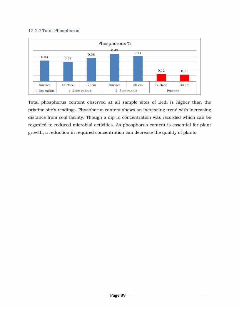
Page 89
12.2.7 Total Phosphorus
Total phosphorus content observed at all sample sites of Bedi is higher than the
pristine site’s readings. Phosphorus content shows an increasing trend with increasing
distance from coal facility. Though a dip in concentration was recorded which can be
regarded to reduced microbial activities. As phosphorus content is essential for plant
growth, a reduction in required concentration can decrease the quality of plants.
0.34 0.32
0.38
0.450.41
0.12 0.11
Surface Surface 30 cm Surface 30 cm Surface 30 cm
1 km radius 1- 2 km radius 2 -3km radius Prestine
Phosphorous %

Page 90
12.3 Mangrove assessment- Bedi
12.3.1 Dust load on leaf
Dust load can accumulate on the leaves due to various processes. The major reasons
for excessive dust load accumulation on leaves is due to anthropogenic activities that
takes places near the vegetations.
Dust load quantification of samples collected at Bedi showed that the amount of dust
found on the leaves was greater on the
samples collected closer to coal storage
facility of port. It also showed a
decreasing pattern in dust
accumulation with increasing distance
from coal handling site of port.
While making comparative analysis of
the samples from pristine location,
higher accumulation of dust was observed on samples of Bedi site. This signifies the
impacts of human activities on leaf dust load which otherwise is found lesser in
natural environment.
12.3.2 Carbon Content Estimation in dust
Carbon content estimation is carried out to get an account of coal dust particles
present in the dust. The coal dust,
dispersed in the air, will settle on
nearby vegetation and can affect it
negatively.
Maximum amount of carbon particles
were found on the samples adjacent to
the coal storage site at Bedi which shown decreasing readings with increase in
distance. This trend indicates that the maximum accumulation of coal dust occurs in
the areas within 1 km radius of the coal handling facility of port. As compared to the
pristine location, having nil carbon particles, the samples of Bedi had considerable
amount of coal dust particles on it.
Figure 12-1: Dust Load on Mangrove Leaf (Bedi)
Figure 12-2: Carbon Content in Dust (Bedi)
8
2.37 2.40.8
100 meters 1000
meters
3000
meters
Control
Dust load(per Cm2)
8
2 2
0
Within 1 km 1 - 2 kmradius
2 - 3 Kmradius
Control
Carbon Content mg/ 50 sq cm

Page 91
43
68
79
95
Within 1 km 1 -2 km radius 2 - 3 km radius Control
Relative Water Content for Bedi %
Figure 12-3: Leaf Chlorophyll Content (Bedi)
Chlorophyll content in the leaves is an indicator of healthy vegetation. The impact of
dust on the leaf was identified by Joshi and Swami in 2009. As per their research, the
accumulation of dust on the leaves reduced the chlorophyll content. Similar
observations were found for the samples collected at Bedi. Chlorophyll content of the
samples with higher dust load and carbon content was minimal. Chlorophyll content
showed an increasing trend as the dust accumulation on the leaves decreased. The
pristine samples had minimum dust load compared to the samples of Bedi and it had
the maximum chlorophyll content which suggests the impact of coal handling activity
of port on the chlorophyll content of the nearby vegetation. The reduced chlorophyll
content affects the vegetation negatively.
12.3.3 Relative leaf water content
Dust applications on excised leaves
of Phaseolus, Coleus and Zebrina
shows increased water loss (Eveling
1969). The research has found that
dust accumulation on vegetation can
significantly increase the process of
water removal in vegetations. The
results of relative leaf water content
analysis show that the moisture
content in the leaf was low in the
Within 1 km 1 - 2 km radius 2 - 3 Km radius Control
Chlorophyll a % 0.42 0.58 0.63 0.9
Chlorophyll b % 0.1 0.15 0.18 0.3
0
0.1
0.2
0.3
0.4
0.5
0.6
0.7
0.8
0.9
1
% C
hlo
rophyll C
onte
nt
Chlorophyll Content % Bedi
Figure 12-4: Relative leaf water content in % (Bedi)

Page 92
samples which had maximum dust load. The samples collected at Bedi port have
relatively lower water content as compared to the pristine samples. The dust load for
pristine samples was also lower to the Bedi samples.
12.3.4 Mangrove density
Figure 12-5: Mangrove density (Bedi)
Figure 12-6: Distribution of mangroves (Bedi)
Bedi site indicates average density of 95.28 plants per 10 m2, showing the similar
trend as Navlakhi port. Class IV and class III tree covers maximum share of 74.38%
surveyed land among vegetation distribution. Share of mature tree of height 1m and
above is 25.62%. Hence Bedi has good capacity of regeneration tress and recruitment
class and indicates higher regeneration potential.
12.3.5 Morphological observation
The quality of mangroves adjacent to the
port was not found in good condition. The
leaf showed blackening due to the
presence of dust. Accumulation of coal
particles on the leaves was clearly visible.
Mangroves at greater distance were in
better conditions and the blackening of
leaves was minimal. The overall condition
of vegetation was not in good state, the
leaves had shown signs of drying and
curling was also observed. This was uniform in all the vegetation where dust
accumulation was higher.
95.28
111.36
80
90
100
110
120
Bedi Pristine
Average mangrove Density per 10m2 - Bedi
36.00% 38.38%
21.94%
3.68%
Class IV Class III Class II Class I
0-60cm 60 -90 1-2 M 2m andAbove
% o
f M
an
gove in
vari
ous
cate
gory
Mangrove height
Distribution of mangroves in %-
Bedi
Figure 12-7: Dust accumulation in 1km

Page 93
12.3.6 Anatomical observation
Anatomy can be correlated with the impacts on growth, though there is no clear
evidence to prove the direct impact. There is slight variation in transverse section and
pith shows some deposition but not of coal particles, whereas there is some difference
in xylem vessels. Anatomical changes are prone to seasonal variations and no
concluding evidence could be found to correlate the impact of coal dust on the
anatomy of the vegetation.
Figure 12-8: Transverse Section Stem (Bedi)
Figure 12-9: Transverse Section Stem (Pristine)
Figure 12-10: Transverse Section Leaf (Bedi)
Figure 12-11: Transverse Section Leaf (Pristine)

Page 94
Figure number 12.11 exhibits prominent coal dust deposition on upper and lower leaf
surface. Coal dust deposition on leaf hair blocks the stomata, in end which hampers
Photosynthetic process of plant (Naidoo G, Chirkoot D, 2004)4.
4 The effects of coal dust on photosynthetic performance of the mangrove, Avicennia marina in Richards
Bay, South Africa.

Page 95
13 Primary data assessment for rozi port
13.1 Physicochemical analysis of Water - Rozi
13.1.1 pH
pH of water sample collected at Rozy port shows
acidic nature with pH value of 6.83. The
permissible limit of water pH should be in range
of 6.5 to 8.5 pH. Thus, the pH of water in Rozy
Port is within the permissible limits.
13.1.2 Total Dissolved Solids (TDS)
Total dissolved solids in the water of Rozy port
were very high measured at 53260 mg/l,
compared to the permissible limits (2100mg/l) for
marine waters.
13.1.3 Turbidity
The water sample collected at Rozy port sites
were fairly clear and had good optical visibility.
The turbidity is also under the permissible limits
of 30 NTU, measured at14.5 NTU.
13.1.4 Chemical Oxygen Demand (COD)
Chemical Oxygen Demand found in the water
samples of Rozy is very high (947.2 mg/l)
compared to the permissible standards of 250
mg/l for marine water.
6.83
8.5
Rozy CPCB Standard
pH
53260
2100
Rozy CPCB Standard
Total Dissolved Solids mg/l
947.2
250
Rozy CPCB Standard
Chemical Oxygen Demand mg/l
14.5
30
Rozy CPCB Standard
Turbidity

Page 96
13.1.5 Biological Oxygen Demand (BOD)
BOD value of marine water near Rozy port is
higher than the given permissible limits of 30 g/l
as it goes up to180 mg/l.
13.1.6 Dissolved Oxygen (DO)
Dissolved oxygen content is the available oxygen
to the marine biota. The water samples collected
at Rozy Port has good amount of DO. The
permissible limit for ecologically important areas
is 5.1 mg/l and the DO values recorded at Rozy
port are 5.1 mg/l.
13.1.7 Phosphate
Samples collected from Rozy port did not show
any significant level of phosphate. The detection
level for phosphate is at least 0.1 mg/l, hence it
can be deduced that the concentration of
phosphate in water is lesser than detection level.
13.1.8 Sulphate
The concentration of sulphate in the water is very
low (157 mg/l) and falls within the permissible
limits of 1000 mg/l.
180
30
Rozy CPCB Standard
Biological Oxygen Demand mg/l
5.1
5
Rozy CPCB Standard
Dissolved Oxygen mg/l
0
3
Rozy CPCB Standard
Phosphate mg/l
157.21
1000
Rozy CPCB Standard
Sulphate mg/l

Page 97
13.1.9 Fluorides
Fluoride content in the water at Rozy Port is
recorded at 2 mg/l which is less than the
permissible limits of 15 mg/l and is not in
quantity to cause any harmful effects on the
marine ecology.
13.1.10 Total Suspended Solids (TSS)
The permissible limits of TSS in water is 100mg/l,
the concentration of TSS in water is clearly above
the permissible limits. The higher concentration of
TSS could affect the ecology negatively, specially
the marine vegetation.
13.1.11 Total Nitrate
Total nitrate in water near Rozy Port is 74.23 mg/l
which is within the permissible limits of 100 mg/l
and will not lead to any ecological impacts if the
current concentration is maintained.
13.2 Physicochemical Analysis of Soil Samples
13.2.1 pH
9 9.1
8.18.3
Surface 30 cm Surface 30 cm
2-3 km radius Prestine
pH
2
15
Rozy CPCB Standard
Fluorides mg/l
160
100
Rozy CPCB Standard
Total Suspended Solids mg/l
47.23
100
Rozy CPCB Standard
Nitrate mg/l

Page 98
The pH of soil samples collected from Rozy showed similar pH value at both surface
and 30 cm layer with 9.0 and 9.1 pH respectively. This shows that the port soil is
comparatively more alkaline than pristine condition. Usually, the pH of soil indicates
little higher alkalinity for marine soils.
13.2.2 Total Nitrate
Total nitrogen content in the surface layer of soil at Rozy Port shows near parity with
the pristine condition but the results of 30cm layer port has shown lesser nitrogen
content compared to the pristine site. Though, the soil nitrogen content for both soil
conditions show near similarity.
13.2.3 Electrical Conductivity (EC)
0.17
0.12
0.16
0.21
Surface 30 cm Surface 30 cm
2-3 km radius Prestine
Total Nitrogen %
1.58
1.26
1.88
1.46
Surface 30 cm Surface 30 cm
2-3 km radius Prestine
Electrical Conductivity ms/cm

Page 99
As compared to the EC of pristine site, soil samples of Rozy Port have indicated lower
EC. But the difference between pristine and Rozy port readings is not significantly
high.
13.2.4 Total Organic Matter
Total organic matter of soil samples collected from Rozy Port was lower than the
organic matter found at the pristine site. The organic matter content observed at Rozy
Port differed at different depth, suggesting accumulation of organic matter for longer
period of time.
13.2.5 Sulphide
Sulphide content in soil differed at different depth and the concentration of sulphide
was comparatively lower than the pristine values. For both samples, majority of
sulphide concentration is found at the surface layer.
1.81
4.08
7.95 8.1
Surface 30 cm Surface 30 cm
2-3 km radius Prestine
Total Organic Matter %
5.83
2.4
6.12
5.32
Surface 30 cm Surface 30 cm
2-3 km radius Prestine
Sulphide ppm

Page 100
13.2.6 Total Potassium
Potassium content for both sites, Rozy Port and pristine location, show near similar
concentration in the soil. And along with this, the difference of potassium at different
depth also doesn’t show any significant difference at both sites.
13.2.7 Total Phosphorus
Phosphorus content in Rozy port’s soil when compared with pristine site, shows
similar concentration values for surface readings. At 30cm level, concentration of
phosphorus decreases at both the sites. Both Rozy and Pristine location soil samples
has recorded near similar amount of phosphorus content.
0.230.24
0.20.19
Surface 30 cm Surface 30 cm
2-3 km radius Prestine
Potassium %
0.26
0.17
0.120.11
Surface 30 cm Surface 30 cm
2-3 km radius Prestine
Total Phosphorus %

Page 101
1.22
0.8
Rozy Control
Dust load Cm2
Rozy Control
13.3 Mangrove assessment
13.3.1 Estimation of Dust Load on Leaf
Dust load is important tool to estimate effect
of pollutants on mangrove ecosystem. Dust
load has negative impact on growth of leaf
and dust load on the surface of leaf alters its
optical properties (Eveling, 1969), hence it
interferes with the normal functioning of the
leaf. Dust load assessment at Rozy Port shows
that there was comparatively more dust on
the leaves of mangroves as compared to the
sample leaves collected from pristine condition5.
13.3.2 Estimation of carbon content in dust particle (mg/50cm2)
Estimation of carbon content in dust was carried out to calculate the amount of coal
particles present in the dust. As there were no mangroves located in nearby areas of
Rozy Port, only one sample was assessed for the carbon content. The sample was
collected from distance of around 3 km from Rozy Port. Moreover, coal export practice
has not been initiated from Rozy port yet, thus there was no trace of carbon content in
dust particles.
13.3.3 Estimation of chlorophyll content
Chlorophyll is the principal photoreceptor in photosynthesis. Its measurement is an
important tool to evaluate the effect of air pollutants on plants, as it plays an
important role in plant metabolism and any reduction in chlorophyll content
corresponds directly to plant growth (Joshi and Swami, 2009).
Figure 13-2: Leaf chlorophyll content (Rozy)
5 Rozy port is an extension of Bedi port. Currently, port has developed only one jetty. There are no mangrove cover in existence in 1 km to 2 Km vicinity of port. Hence, mangrove sample has been collected from only one location (at 3 Km distance). However, Rozi port has not initiated coal exports. As result, mangrove samples do not exhibits any coal dust
trace.
Figure 13-1: Dust Load on Leaf (Rozi)

Page 102
Chlorophyll content of samples collected at Rozy were marginally lower compared to
the chlorophyll content of pristine samples. Dusted leaf surface causes reduction in
chlorophyll content and is further responsible for reduction in the photosynthesis
activity in leaf (Joshi and Swami, 2009).The difference of dust load on samples
collected at both Rozy and pristine site were marginal, where Rozy port samples had a
slightly higher dust load compared to pristine conditions. The chlorophyll content has
also shown similar results which indicates that dust load has negative impacts on the
chlorophyll content which is declining in samples collected from Rozy Port.
13.3.4 Estimation of relative leaf water content
As per Eveling 1969, dust particles have triggered an increased loss of water from the
leaves. Relative leaf water content
estimates the amount of water
moisture present in the leaves which is
important for mangrove health and
quality. The samples collected at Rozy
Port have shown lower leaf water
content as compared to pristine
samples. This correlates with the
amount of dust load found on the
leaves of both sites. Though the moisture content in the samples was not significantly
low compared to the pristine samples and the sample leaves showed a good amount of
moisture in it.
85
95
2 - 3 km radius Control
Relative Water Content for Rozy %
Figure 13-3: Relative leaf water content (Rozi)

Page 103
13.3.5 Mangrove density
Figure 13-4: Average mangrove density
per 10m2 - Rozi
Figure 13-5: Distribution of mangroves in - Rozi
Rozy site has indicated the highest average tree density of 102.59 plants per 10 m2,
surpassing all surveyed sites and resembling it closely with pristine. Matured trees’
(1m & above) share in total surveyed area is at 47.18% which is also highest among all
surveyed sites. Class IV and Class III tree cover 31.43% and 21.39% of surveyed area
respectively.
13.3.6 Morphological Observations
Overall appearance of mangroves near
Rozy port site was healthy with good
quality of leaves. The leaves had bright
green color and no blackening was
observed on the leaves which suggest
that there would be no accumulation of
coal dust on leaves. Overall cover of
mangroves was dense and populated
with healthy mangroves. The leaves did
show a bit of curling, but no indicators
where found which suggests any
negative impact on the health of mangrove at Rozy Port.
102.59
111.36
95
100
105
110
115
Rozi Pristine
Average mangrove Density per 10m2 - Rozi
31.43%21.39%
41.33%
5.85%
Class IV Class III Class II Class I
0-60cm 60 -90 1-2 M 2m andAbove
% o
f M
ango
ve in
va
rio
us
cate
gory
Mangrove height
Distribution of mangroves in %- Rozi
Figure 13-6: Mangrove Leaves at Rozy Port

Page 104
13.3.7 Anatomical Observations
Figure 13-7: Rozy Transverse Section of Stem
Figure 13-8: Pristine Transverse Section of Stem
There is no difference in pith, palisade tissue in T.S of leaves. There is no difference in
pith, xylem vessel in T.S of stem at Rozy as compared to pristine. There is slight
variation in anatomy of both leaf and stem section compared to the sections of
samples collected from pristine location, but to reach up to any conclusion based on
such variations will not be justifiable scientifically. There are lots of environmental,
climatic, ecological parameters that can alter the anatomy of the plant.
Figure 13-9: Rozy Transverse Section of Leaf
Figure 13-10: Pristine Transverse Section of Leaf
Dust traces are found on upper surface of leaves but no coal substance contamination
observed in dust particles. Since, coal export/import is not being operated on Rozi
port, coal dust impact is nil.

Page 105
14 Coal deposition on stomata and Stomata Density
Analysis
14.1 Coal dust accumulation on stomata
Assessment was carried out to substantiate evidence of coal dust impact on leaf. Since
coal dust deposition is highest on leaves, prior impact can be seen on stomata through
coal dust accumulation on stomata. Hence, determining alteration in anatomy with
specific focus on stomata was crucial requirement. Leaves section collected from all
the study sites were analysed through electron microscope.
Stomata is small apertures on the leaf surface that regulate loss of water via
transpiration and CO2 uptake during photosynthesis, and thereby water relation and
plant biomass accumulation is influenced by stomata movement (Al Afas et al. 2006;
Bussis et al. 2006). Stomata may occur on both the side of the leaves such leaves are
called amphistomatus leaves.
Figure 14-1: Lower Epidermis of leaf collected from Bedi

Page 106
Figure 14-2: Lower Epidermis of leaf collected from Kandla
Figure 14-3: Lower Epidermis of leaf collected from Navlakhi

Page 107
Figure 14-4: Lower Epidermis of leaf collected from Rozi
After examining the lower epidermal layer of mangove it was clear that the dust
accumulation was present and dust particles obstructed the stomata’s opening. Dust
particles can be clearly seen in all the samples with maximum accumulation can be
seen in samples collected from Bedi, and Navlakhi . Samples collected from Rozy and
Kandla demonstrates negligible dust accumulation along with pristine location.
According Joshi and Swami in 2009, Shamaila Zia-Khan- 2015, dust accumulation on
leaves reduces chlorophyll content and photosynthesis process.
14.2 Stomata density
Stomatal density is the count of stomata per unit area of the leaves and for the study
of stomatal density the samples collected where studied under scanning electron
microscope and the number of stomata where calculated per unit area.
Sample Stomatal Density (Number of
stomata/mm
Pristine 11

Page 108
Bedi 17
Kandla 24
Navlakhi 16
Rozy 13
Results of stomatal density analysis revealed that the count of stomata increased in
the areas that are nearer to the coal handling sites, compare to samples collected from
the pristine site. It is observed that stomata density was more for the samples which
had more dust cover on the leaves compared to the pristine location where dust load
was less.
According to hamaila Zia-Khan 2015, Eller 1977, dust particale deposition lead to rise
in leaf temperature. however, temperature is positively correlated with stomata, and
increase in temperature elevate in stomata density. A similar phenomenon was found
during the stomata density assessment. Leaves with higher coal dust have exhibited
greater number of stomata density.

Page 109
15 Heavy Metal Assessment
Heavy metals are elements having relatively higher atomic numbers and are metallic
in nature, often considered as a polluting agent for the environmental studies. As a
decomposition product of ancient plants, coal contains virtually every element found
in living plant tissues, including trace metals. Metals may be present as dissolved
salts in pore waters, as metallo-organic compounds, or as mineral impurities (e.g.,
iron in pyrite, FeS, and zinc in sphalerite, ZnS). Information on trace elements in coal
has been reviewed comprehensively by Swaine (1990) and Swaine & Goodarzi (1995),
including environmental aspects during mining and combustion.
The concentration of heavy metal in coal can vary and the presence of particular heavy
metal may also very. So far all the major heavy metals have been found present
through the secondary data assessment and literature review. This segment discusses
the results of heavy metal assessments for soil and water at different sites.
15.1 Heavy Metal Assessment for Water Samples
Water samples analysis for the presence of heavy metal showed no significant
presence of any heavy metal in the water. All major heavy metals assessed showed
negligible concentration and were below detection levels. Hence heavy metal
assessment doesn’t prove any significant contamination in the water at all the
identified sites. The information about the detection levels for all the heavy metals that
were assessed is given in the table below:
Table 15-1: Detection levels for all the heavy metals
Parameters Detection levels
Selenium mg/l 0.01
Iron mg/l 0.08
Cadmium mg/l 0.0005
Mercury mg/l 0.005
Copper mg/l 0.04

Page 110
Chromium mg/l 0.03
Arsenic mg/l 0.005
Zinc mg/l 0.01
Lead mg/l 0.005
Nickel mg/l 0.01
15.2 Heavy Metal Assessment of Soil
The results of heavy metal analysis of soil showed contamination of 6 different heavy
metals in the soil. Presence of heavy metal like selenium, cadmium, mercury and
arsenic were not found in any soil samples or the concentration was below detection
levels. All soil samples including the pristine location showed presence of lead, zinc,
copper and iron. Only samples collected from Navlakhi Port showed the presence of
chromium and nickel in addition to above mentioned heavy metals. This segment
discusses the presence of heavy metal in the soil for different ports.
Kandla Rozy Bedi Navlakhi Pristine
Surface 30
cm
Surface 30
cm
Surface Surface Surface 30
cm
Lead ppm 6.4 6.8 6.84 6.24 6.31 10.39 3.12 3.05
Zinc ppm 81.04 70.62 74.32 81.83 78.34 110.72 71.21 72.24
Copper
ppm
7.2 6.1 5.32 5.92 5.32 18.22 2.11 2.09
Iron ppm 5.24 5.8 6.82 6.82 6.98 11.37 3.25 3.21
Chromium
ppm
nil nil nil nil nil 3.44 nil nil
Nickel
ppm
nil nil nil nil nil 1.49 nil nil

Page 111
Heavy Metal Assessment for Lead
Concentration of lead was found in all sites including the pristine location, the
concentration of lead for all sample sites was found to be similar (in the range of 6% to
7%) except for Navlakhi which showed 10.39% of lead content. Lead content in soil
can have toxic effect to the ecology and can affect the environment negatively. As there
are no standards available for the permissible limits of lead in the soil, it is difficult to
conclude the significance of lead content found.
Heavy Metal Assessment for Zinc
In all samples, concentration of Zinc was highest compared to other heavy metals.
Zinc contamination was found in all sample sites. Navlakhi showed the maximum zinc
content as compared to the other ports and pristine samples together. Among other
ports, the content of zinc ranged from 81.04 to 70.62.
81.0470.62 74.32
81.83 78.34
110.72
71.21 72.24
Surface 30 cm Surface 30 cm Surface Surface Surface 30 cm
Kandla Rozy Bedi Navlakhi Pristine
Zinc
6.4 6.8 6.84 6.24 6.31
10.39
6.12 6.05
Surface 30 cm Surface 30 cm Surface Surface Surface 30 cm
Kandla Rozy Bedi Navlakhi Pristine
Lead

Page 112
Heavy Metal Assessment of Copper
Copper content was observed in soil samples. Its concentration was significantly high
for Navlakhi Port soil samples compared all other ports’ soil samples. Rest, all ports
had similar concentration of copper with marginal variation, including the soil
samples collected from pristine location.
Heavy Metal Assessment for Iron
Soil samples from all the sites including the soil sample of pristine location shows the
presence of iron in soil. The content of iron was similar for all soil samples including
pristine. Navlakhi Port showed the maximum concentration of iron compared to other
samples.
7.26.1 5.32 5.92 5.32
18.22
5.11 5.09
Surface 30 cm Surface 30 cm Surface Surface Surface 30 cm
Kandla Rozy Bedi Navlakhi Pristine
Copper
5.24 5.86.82 6.82 6.98
11.37
5.25 5.21
Surface 30 cm Surface 30 cm Surface Surface Surface 30 cm
Kandla Rozy Bedi Navlakhi Pristine
Iron

Page 113
Heavy metals assessments have shown that 4 major heavy metals were found in the
soil samples. And, water samples didn’t record any heavy metals (or the concentration
of heavy metal was below detection levels. All sites have a similar content of heavy
metal including Rozy port though no coal is being traded or handled from Rozy port. It
suggests that the availability of heavy metal in the soil samples of Rozy port might be
due to other industrial/anthropogenic activities other than coal handling.
The presence of heavy metal in the soil or nearby environment can pose a risk on the
health of vegetation. All four identified heavy metals have poisoning tendency at a
higher concentration. Higher Cu level inhibits growth, reduces metabolic activities of
the plants and also affects the chlorophyll content in the vegetation (Rousos and Palta,
1986; Maskmiec and Baszynski., 1995 and Maksymiec., et al. 1994). Higher levels of
zinc in the environment can affect the yield of vegetation, reduces the photosynthesis
capacity of the plant and can lessen the auxin production (Brain., 2005).
Mangroves are species tolerant to heavy metal contamination and can also control
some heavy metal contamination naturally. As per the research done by Lindsey et al.
2005, A. marina roots exhibited highest Pb metal value causing it more effective in
reducing of the contaminant material of the Pb metal.

Page 114
16 Coal dust control Measurement
Dust control / management measurement should be adapted which recognize and
responds to the issue of dust emissions at all stages from loading, transporting to
storage. This section of the report outlines an approach for implementing a dust-
management system incorporating best environmental management practices for
managing dust from coal mining operations.
Dust sources
When handling coal, there are a number of sources of dust, and all need to be
addressed to arrive at an environmentally sensitive and professional operation. For an
unloading operation these sources are:
Unloading at the ship
Reception at the wharf side
Conveying transfer points
Open belt conveying at height
Drop from conveyor to stockpile
Time spent as a stockpile
Vehicle movements around stockpile
Transfer to onward transport.
Dust control measures can largely divided in three segments:
1) Dust collection system
2) dust suppression system
3) Conveyor covers
Dust collection system
Dust collection systems use ventilation principles to capture the dust-filled air-stream
and carry it away from the source through ductwork to the collector. This involves
passing the air carrying dust from the source through a filtration system. There are
passive systems, which merely allow the air to pass through the filters, and active
systems, which pull the air in (like a vacuum cleaner) to remove solids.

Page 115
Conventional collection systems use slight
negative pressures created by air movement to
transport airborne particles through ducts to a
central collection point. Capture hoods are
located in areas where dust is generated and
the hoods transport it through ductwork to a
central collection point.
A typical dust collection system consists of four
major components, such as (1) An exhaust hood to capture dust emissions at the
source; (2) Ductwork to transport the captured dust to a dust collector; (3) A dust
collector to remove the dust from the air; (4) A fan and motor to provide the necessary
exhaust volume and energy.
Figure 16-1: Typical design of wet centrifugal dust collector
Wet centrifugal dust collector uses scrubbing effect of water to suppress dust. Water is
very good binding substance for dust, thus it is used as scrubbing element. This
device applies the principle of film formation over the dust layer and it confines dust
particles, leaving fresh air to escape. Dust collector shown in figure 4 discusses its
simple design, in which radically inward fans produce very high suction pressure
powered by 2hp motor. The power capacity of motor varies as per requirement. This
device uses the principle of dynamic precipitation technique in which very high
suction pressure suck the dusty air and allow to centrifuge through it. Centrifugal

Page 116
action separates dust from fresh air, and then fresh air is allowed to escape from other
end of dust collector.
The dust collector has a small tank full of water which has two valves. These two
spring-loaded valves are operated to allow passage of concentrated dust and automatic
filling of fresh water using sensors. These sensors sense the concentration level of dust
in the container and when concentration goes beyond 90%, it opens the discharge
valve. This remains open until total concentrated dust is discharged from the tank. At
the same time, it opens inlet valve to allow fresh water to fill up. The dust collector
uses automatic discharge technique and hence save time for manual operations of
discharging and refilling. Also, this discharge is recycled in order to have minimum
water wastage. This centrifugal dust collector is very efficient and requires minimum
amount of water since it discharges dust in concentrated form.
Dust suppression system
Dust suppression is the technique which uses water or chemically treated water in
spray or fog formation to prevent the fine particulates emitting the surfaces of haul
roads, stockpiles, conveyors, dump hoppers etc. into air. There are a number of
mechanical systems used for this purpose, ranging from water carts and manually
operated sprinklers to automated sprinkler systems triggered by wind speed or
vibration.
Wet dust suppression techniques use water sprays to wet the material so that it
generates lesser dust. There are two different types of wet dust suppressions: (i) wets
the dust before it is airborne (surface wetting) and, (ii) wets the dust after it becomes
airborne. In many cases, surfactants or chemical foams are added to the water in
order to improve efficiency. A water spray with surfactant means that a surfactant has
been added to the water in order to lower the surface tension of water droplets, allow it
to spread further over material and also deepen its penetration into material.
A) Surface wetting system
The principle behind surface wetting is the idea that dust will not even be given a
chance to form and become airborne. With this method, effective wetting of the
material can take place by static spreading (wetting material while it is stationary) and
dynamic spreading (wetting material while it is moving). For static wetting, more

Page 117
effective dust suppression can be achieved by increasing the surface coverage either
reducing the droplet diameter or its contact angle. For dynamic spreading, more
factors come into play such as the surface tension of the liquid, droplet diameter, size
of the material being suppressed and droplet impact velocity.
B) Airborne dust capture system
Airborne dust capture systems may also use a waterspray technique; however,
airborne dust particles are sprayed with atomized water. When the dust particles
collide with the water droplets, agglomerates are formed. These agglomerates become
too heavy to remain airborne thus they settle. Research indicated that, if a sufficient
number of water droplets of approximately the same size as the dust particles could be
produced, the possibility of collision between the two would be extremely high. It was
also determined that if the droplet exceeded the size of the dust particle, there would
be little probability of impact and the desired precipitation. Instead, the dust particle
would move around the droplet.
There are three common methods for wet dust suppression.
A) Fog
User: wharf side reception hoppers; conveyor transfer points, stockpile building,
wagon loading
Fogging works by releasing very small droplets of water into air. Airborne dust
particles adhere to the water droplet and form agglomeration. Once several have
agglomerated together, they become heavy enough to fall out of the air. The water
droplet size is very important. If the droplet is too large, e.g. 50 microns and above, the
dust particle will bounce off the water droplet surface tension and remains airborne.
To achieve a useful dust suppression effect, the droplets need to have a mean
diameter in the region of 10 to 15 microns, i.e. similar to the size and mass of
respirable dust particles. If the fog is generated in the right way, by using pressurised
water, the energy required can be very low – between 2 to 3kW for a system requiring
hundreds of nozzles, e.g. a large stockpiler tripper conveyor – giving considerable
operating cost savings when compared to other techniques.

Page 118
B) Water Sprinklers
Uses: stockpiles and haul-ways
Once stockpiled, water can be sprayed on the stockpiles to keep them damped down.
Sprinklers should be used with caution, however, as the volume of water required can
be significant, causing drainage and run-off treatment into problems. Irrigation
systems can be used to control dust on
outdoor stockpiles, but when the
stockpiles are excavated, dust will arise
as the drier material in the pile is exposed
and moved around. The sprinkler droplet
sizes are often in excess of 100 microns,
which is too large to suppress airborne
dust, and it is quite common to observe
dust rising from the ground where the
sprinkler water lands, thus exacerbating the problem! An irrigation system uses a lot
more water than a fogging system – typically 10 times the amount – and is much less
effective when materials are being moved around. Sprinklers should be used as a last
line of defence and with considerable planning and forethought.

Page 119
C) Surfactants
Uses: haul-ways and stockpiles
To reduce the amount of water used with sprinklers, adding chemicals that improve
the penetration and wetting effect of the
water is possible. This can be especially
useful on haul-ways, where regular vehicle
movements stir up dust regularly. The
proper use and application of surfactants
can halve the number of times that a surface
has to be treated. There are a number of
ways they can be applied:
a. An additive to a sprinkler system
b. Application from a pumped hose and mobile bowser
c. Sprinkling as dry granules.
Conveyor covers
Uses: all transfer conveyors
When material is being conveyed from one point to another, cross-winds over the
conveyor can cause dust to be lifted. It is therefore essential to ensure that all
conveyors are covered. This can be done simply with covers fitted over the conveyor
belt, such as the Traffield Conveyor covers available from Renby. For a tripper
conveyor, as the belt is lifted at the moving discharge point, the top of the conveyor
cannot be covered as easily, so wind boards should be fitted to keep wind off the belt.

Page 120
17 Discussion
The present study is aimed at understanding the impacts of coal dust on the
mangrove ecology. While studying ecology, it becomes imperative to examine all
parameters pertaining to it rather than focusing on single indicator. Thus, to identify
the impacts of coal dust on mangrove, we obtained the holistic approach by studying
not only mangrove physiology but as well the physiochemical indicators (soil & water)
and heavy metal assessment. The purpose of examining the physiochemical indicators
is the ideal first step in ecological study to assess whether the state of soil and water
in sample geographical area is meeting the standards to create favorable environment
for ecology to flourish or not. Such examinations give an overall view of anthropogenic
influence on physiochemical parameters of marine environment though it is not
possible to distinguish and determine the intensity of each anthropogenic activity’s
impact. Thus, the physiochemical assessment was conducted since it gives insights
into the contamination levels of sample site and knowing such status before initiating
the mangrove ecology study is essential.
The direct impacts of coal dust on mangrove were visible and derived further by
observing the physiological and anatomical state of mangrove. But such observation
may vary since it is completely dependent on the geographical locations and
time/season of sample collection. Moreover, the role of coal dust in overall impacts on
mangrove cannot be ascertained since there are other natural and anthropogenic
factors affecting the mangrove physiology. Additionally, the mangrove natural
regeneration was observed at all sample sites. Since mangrove has bioremediation
characteristic, it tends to absorb the additional nutrient flow (containing heavy metal)
coming in from human activities which may have led to its proliferation.
The physiochemical indicators for water and soil were studied while comparing it with
the CPCB standards as benchmarks. And it was observed that TDS, having
permissible limits of 2100 mg/l, was above the benchmark ranging from 24420 mg/l
to 39700 mg/l and Kandla reported the highest concentration among all observed port
sites while Bedi being minimum. The COD level was also exceeding the allowed limit of
20 mg/l in Kandla whereas it was contained in Rozy, Bedi and Navlakhi sites. For
TSS, only Kandla recorded exceeding the 100 g/l limits while other sample sites
indicated TSS within permissible limits. The BOD levels in Kandla & Rozy were above

Page 121
permissible limit and Navlakhi & Bedi recorded within limit levels. Nitrate and
Sulphate levels at Bedi shows highly elevated concentration compared to other ports.
The elevated level of Sulphate can be due the presence of coal dust in the
environment.
Heavy metals in water are below detection levels for all the water samples taken from
sample sites. This can be due to high dilution/churning of sea water. Lead, zinc,
copper and iron from soil samples were detected in all study sites. Lead contamination
varies from 10.39 ppm to 6.4 ppm whereas Zinc ranges from 110 to 81 ppm. Navlakhi
has the recorded highest contamination level of all heavy metals and it is the only site
which recorded the presence of Nickel and Chromium.
The mangrove physiological assessment indicated the presence of coal dust on leaves,
ranging from 1.2 mg/cm2to 1.8 mg/cm2. The highest dust load on leaves was observed
at Navlakhi and lowest at Roz site.
The carbon content analysis revealed the highest readings for Bedi port and it was
also observed that the carbon content level decreases gradually as we analyse the
samples collected from distant sites. Maximum carbon content is found in samples
collected from 1km periphery of coal handling site. The relative water content of
mangrove leaves was recorded lowest at Kandla and Bedi, varying from 43 to 70%. The
chlorophyll content analysis indicated the lowest content in samples collected from
Kandla and Bedi sites at 45% and 42% respectively whereas Rozy and Navlakhi sites
recorded 70% and 58% respectively.

Page 122
18 Conclusion
Environmental status plays a very important role in understanding the health of any
particular ecosystem. Physicochemical analysis of soil and water carried out for the
mangrove ecosystem showed contamination of different types but correlating it with
coal as its major source can’t be established since there are various other
developmental activities taking places around port which could have contributed to
the pollution. Correlating physicochemical changes and heavy metal contamination to
mangrove health is also difficult as there is existing research gaps on this subject.
Thus, there is no established research methodology or standards which can ascertain
the impact of heavy metal contamination on mangrove or mangrove ecology.
Results of soil and water samples’ analysis revealed that the samples collected around
Kandla Port and Bedi Port showed highest variation in the physicochemical properties
of soil and water. Heavy metal contamination was observed in all sites including the
pristine location but Navlakhi has the maximum contamination amongst all the ports.
Navlakhi is also the only port which detected chromium and nickel in the soil.
Physicochemical and heavy metal analysis shows signs of environmental pollution
around all the ports. Physiological analysis of mangrove samples revealed a high
degree of impact in Kandla and Bedi. The impact is focused and is observed maximum
up to 1 kilometer periphery from coal handling site at port, the impact intensity
decreases as the distance from the port increases. Beyond 3 kilometer periphery, the
impact observed is very low.
Impacts observed at Kandla can’t be explained solely due to the coal dust
contamination but port extension activities also have impact on the mangrove cover
around the port. Mangroves around Bedi Port had a high quantity of coal dust particle
observed due to coal dust but such condition can be reduced at Bedi if proper dust
reduction measures are taken.
Changes in mangrove health are dependent upon many factors such as climate,
environment, nutrient availability etc. So to find out specific impact, robust
methodology and framework is needed to be developed. Development of such methods
will support assessment of coal to firmly provide results on the impacts of coal on
mangrove. Stomata blocking and reduction in chlorophyll content seems to be getting
directly hampered from coal dust. But to create a deeper understanding, further

Page 123
studies should be carried out covering all seasons& geographical locations to find out
the magnitude and the temporal nature of the impact. It is highly recommended that
such study, sampling and data generation should be carried out for all the three
seasons including flowering period.

Page 124
19 Bibliography
A., J. P. (2009). Air pollution induced changes in the photosynthesis pigments of
selected plant species. Journal of Environmental Biology , 30(2), 29-298.
Agency, C. E. (1996). A guide on biodiversity and environmental impact assessment. .
Ottawa Minister of Supply and Services.
Airoldi, L. (2003). The effects of sedimentation on rocky coast assemblages.
Oceanography and Marine Biology: An Annual Review , 41, 161-236.
Airoldi, L. (2003). The effects of sedimentation on rocky coast assemblages.
Oceanography and Marine Biology: An Annual Review , 41, 161-238.
Al Afas, N., Maroon, N., & Ceulemans, R. (2006). Clonal variation in stomatal
characteristics related to biomass production of 12 popular (Populus) clones in a short
rotation coppice culture. . Environmental and Experimental Botany, 8: , 279-286.
Allen, J. R. (1987). Coal dust in the Severn Estuary, southwestern UK. Marine Pollution
Bulletin , 18, 169-174.
Alloway, B. J. (2008). Zink in soil and crop. Nutrition , 32-35.
Assessment), I. (. (2001). Proposed conceptual and procedural framework for the
integration of biological diversity consideration with national systems for impact
assessment.
Atkinson, S. F. (2000). Treatment of biodiversity impacts in a sample of US
environmental impact statements. . Impact Assessment and Project Appraisal 18(4) ,
271-282.
Bussis, D., Von Groll, U., Fisahn, J., & Altman, T. (2006). Stomtal aperture can
compensate altered stomatal density in Arabidopsis thaliana at growth light
conditions. Functional Plant Biology, 33. , 1037-1043.
Byron, H. J. (1999). Biodiversity issues in road environmental impact assessments:
guidance and case studies. In: Evink G.L., P. Garrett and D. Zeigler, eds.,. Proceedings
of the Third International Conference on Wildlife Ecology and Transportation.
Tallahassee: Florida Department of Transportation .
Byron, H. J. (2000). Road developments in the UK: An analysis of ecoological
assessment in environmental impact statement produced between 1993 and 1997.
Journal of Environmental Planning and Management 43(1) , 71-97.

Page 125
Dalal-Clayton, B. (1992). Modified EIA and indicators of sustainability: first steps
towards sustainability analysis. London: International Institute for Environment and
Development .
Diamantini, C. B. (2000). Planning the urban sustainable development. The case of
the plan for the province of Trento, Italy. . Environmental Impact Assessment Review
20, , 299-310.
Diamantini, C. B. (2000). Planning the urban sustainable development. The case of
the plan for the province of Trento, Italy. Environmental Impact Assessment Review 20,
, 299-310.
Eller, B. (1977). Road dust induced increase of leaf temperature. Environ. Pollut., , 93-
107.
Eveling, D. W. (1969). Effects of spraying plants with suspensions of inert dust. Ann.
Appl Biol., , 64, 139-151.
Ferrini, V. L. (2001). Sedimentary characteristics and a acoustic detectability of ship
derived deposits in western Lake Ontario. Journal of Great Lakes Research 27, , 210-
219.
Ferris, R. N. (1996). Elevated CO2 and temperature have different effects on leaf
anatomy of perennial rye grass in spring and summer. Ann. Bot. 78, , 489-497.
French, P. W. (1993). Post-industrial pollutiant levels in contemporary Severn Estuary
interidal sediments comapred to pre-industrial levels. Marine Pollution Bulletin , 26,
30-35.
Georce, C. (1999). Testing for sustainable development through environmental
assessment. . Environmental Impact Assessment Review 19, , 175-200.
George, C. (1980). Ecological assessment for regional development. Journal of
Environmental Management 10 .
George, C. (2000 a). Environmental impact prediction and evaluation. In: Lee N. and
C. George, eds., Environmental assessment in developing and transitional countries.
Chichester:. Wiley, , 8-110.
George, C. (1999). Testing for sustainable development through environmental
assessment. . Environmental Impact Assessment Review 19 , 17-2000.
Lake, R. G. (1999). Acute impact of suspended sediment angularity on juvenile coho
salmon (Oncorhynchus kisutch) . Can. J. Fish. Aquat. Sci. 56, , 862-867.
Limpenny, D. R. (1992). Environmental Impact of marine colliery waste disposal
operations on the sea bed off Seaham, County Durham. Lowestoft. U.K.: Ministry of
Agriculture, Fisheries and Food, directorate of Fisheries Research .

Page 126
Lindsey H. Defew, J. M. (2005). An assessment of metal contamination in mangrove
sediments and leaves from Punta Mala Bay. Pacific Panama, Marine Pollution Buletin ,
0, 547-552.
Maksymiec W., R. R. (1994). Effect of excess Cu on photosyntheisis apparatus of
runner bean leaves treated at different growth stages . Physiol Plant , 91, 715-721.
Maskmiec W, B. T. (1995). The influence of Ca2+ on toxicity ectent of Cu2+ action on
runner bean plants at different growth stages of thier primary leaves. Bio Bull Poznan
32(Suppl.) , 40.
McManus, J. (1998). Temporal and spatial variations in estuarine sedimentation.
Estuaries , 21, 622-634.
Moore, P. G. (1977). Inorganic particulate suspensions in the sea and their effects on
marine animals . Oceanic and Marine Biology: An Annual Review , 22-363.
Moore, P. (1977). Inorganic particulate suspensions in the sea and their effects on
marine animals. Oceanography and Marine Biology: An Annual Review , 1, 225-363.
Norkko, A. H. (2001). Benthic-pelagic coupling and suspension-feeding bivalves:
linking site specific sediment flux and biodeposition to benthic community structure. .
Lommology and Oceanography 46 , 2067-2072.
Noss, R. F. (1994). Saving nature's legacy, protecting and restoring biodiversity.
Washington D. C.: Islan Press .
Patel Ajay1, S. V. (2014). Mapping and Monitoring of Mangroves in the Coastal Districts
of Gujarat State using Remote Sensing and Geoinformatics,. Ghandhinagar:
Bhaskaracharya Institute for Space Applications and Geo-informatics (BISAG) and
Gujarat Ecological Commission (GEC).
Pearce, D. (1993). blueprint 3. Measuring sustainable development. London: Earthscan
.
Reddy, k. R. (1998). Interactions of CO2 enrichment and temperature on cotton
growth and leaf characteristics. . Environ. Exp. Bot. 39, , 117-129.
Reid, D. F. (1999). Proceedings of the Workshop: The Environmental Implications of
cargo sweeping in the Great Lakes. NOAA Technical Memorandum ERL GLERL , 114.
Rousos, P. A. (1986). Reduction of chlorophyll in cabbage leaf disks following Cu2+ .
Expoure.- Hort Science , 21: 499-201.
Shamaila Zia-Khan., W. S. (2015). Effect of dust deposition on Stomatal conductance
and leaf. . Water, 7. , 116-113.

Page 127
Swaine, D. J. (1995). Environmental Aspects of Trace Elecments in coal. Kluwer
Academic, Dordrecht, Netherlands , 324.
Swaine, D. J. (1990). Trace elements in coal. Butterworth, London , 278.
Wagner, F. (1998). The influence of environment on the stomatal frequency in Beutal,.
LPP Contrib. Series 9, .
Williams, R. &. (1974). The fish population of an industrial river in South Wales .
Journal of Fish Biology , 6, 395-414.


