1 FINAL REPORT DIAGNOSIS AND REMEDIATION OF SUSTAINED CASING PRESSURE IN WELLS Andrew K. Wojtanowicz, Somei Nishikawa, and Xu Rong Louisiana State University Submitted to: US Department of Interior Minerals Management Service 381 Elden Street Herndon, Virginia 20170-4817 Baton Rouge, Louisiana July 31, 2001
Transcript
1
FINAL REPORT
DIAGNOSIS AND REMEDIATION OFSUSTAINED CASING PRESSURE IN
WELLSAndrew K. Wojtanowicz, Somei Nishikawa, and Xu Rong
Louisiana State University
Submitted to:
US Department of InteriorMinerals Management Service
381 Elden StreetHerndon, Virginia 20170-4817
Baton Rouge, LouisianaJuly 31, 2001
2
TABLE OF CONTENT
PageEXECUTIVE SUMMARY 31. BACKGROUND OF SCP DIAGNOSIS AND REMOVAL 42. CURRENT PROCEDURES FOR SCP TESTING3. FIELD DATA ANALYSIS 6
3.1 SCP Data Bank 63.2 Statistical Analysis 6
3.2.1 SCP Occurrence 63.2.2 SCP Magnitude by Casing String 7
4. ANALYSIS OF SCP PRESSURE TESTING MECHANISM 105. MATHEMETICAL MODELS OF SCP BUILDUP 12
5.1 Analytical Model of SCP Transient in Annulus Cemented to Surface 125.2 Numerical Model of SCP Buildup in Cemented Annulus with Mud Column 13
6. EFFECT OF WELL PARAMETERS ON CASINGHEAD PRESSURE BUILDUP 146.1 Wellhead Pressure Transient Behavior in Fully Cemented Annulus 146.2 Pressure Buildup in Cemented Annulus with Mud Column 16
7. METHOD FOR SCP DIAGNOSIS 197.1 Validation of Numerical Model with Field Data 19
7.1.1 Case 1: Partial SCP Buildup Data 197.1.2 Case 2: Complete SCP Buildup Data 21
7.2 Diagnostic Software and Applications 228. SCP DIAGNOSIS - CONCLUSIONS AND RECOMMENDATIONS 239. CURRENT STATUS OF SCP REMMEDIATION - CYCLIC INJECTION 2510. EXPERIMENTAL ASSESSMENT OF CYCLIC INJECTION 26
10.1 Experimental Design 2610.1.1 Physical Model 2610.1.2 Data Analysis Method 2910.1.3 Selection of Displacing Fluids 3310.1.4 Testing Procedure 34
11. SCP REMEDIATION – CONCLUSIONS AND RECOMMENDATIONS 45BIBLIOGRAPHY 46
APPENDIX A: SCP DATA BANK 48APPENDIX B: ANALYTICAL MODEL OF SCP TRANSIENT
IN ANNULUS CEMENTED TO SURFACEAPPENDIX C: NUMERICAL MODEL OF SCP BUILDUP IN
CEMENTED ANNULUS WITH MUD COLUMNAPPENDIX D: RESULTS OF.CYCLIC INJECTION EXPERIMENTS
3
EXECUTIVE SUMMARYReported herein is a research project performed under TASK 2A - Remediation of Flow AfterCementing of the project “Development of Improved Procedures for Detecting and HandlingUnderground Blowouts in a Marine Environment.” The task has been added to the projectprogram based upon modifications proposed by LSU in a letter to MMS, October 3, 1988, andapproved by MMS on October 19, 1998.
This new task was intended to be a follow-up to Task 2, “Prevention of Flow AfterCementing,” and Task 11, “Study of Excessive Casing Pressures During Production Operations.”A need for this new task arose from recent industry engagement in deep-water operations and thegrowing concern of MMS about sustained casing pressures (SCP). The overall objectives of thistask were to identify theoretical principles and to conduct research into new technology fordiagnosis and removal of SCP in producing wells.
The report on the first stage of this project, diagnosis and testing of SCP, presents theanalysis of operator field testing procedures and the MMS guidelines for testing wells with SCPand includes data collected from field testing and monitoring SCP along with an analysis oftypical recorded patterns of SCP buildup during the field tests.
The report on the theoretical stage of the project describes two mathematical models:pressure transient in a fully cemented annulus ; and SCP buildup in a well with a mud columnabove the cement. The models were used to study the effects of well properties on SCPdevelopment patterns. Based upon the study, a computer-assisted method for SCP diagnosis wasdeveloped and validated using the field data; the software for this application is attached to thereport. The report also includes examples for using the software.
The report on the experimental stage of the project addresses the most critical problem inremediation of SCP without using a drilling/workover rig: injection of high-density fluid into theaffected annulus in order to kill SCP. The fluid is injected either at the surface directly into thecasinghead (Bleed-and-Lube method) or through a flexible tubing inserted to a certain depth inthe annulus (Casing Annulus Remediation System, CARS). Given the depth limitation of CARS,the two methods are similar in applying multi-cyclic injection of heavy liquid to kill SCP in theaffected annulus. The objective of this portion of the study was to evaluate the efficiency ofdisplacing annular fluid with injected fluid during cyclic injection.
A pilot-scale physical model of the well annulus was built and used for studying heavyfluid settling and displacement performance. The experimental matrix considered miscible andimmiscible variants of the two fluids (displacing and annular) and included calcium carbonatebrine, water-based mud, water, and white oil in various combinations.
The results showed that using brine with drilling mud may by entirely ineffective,particularly when high concentrations of clay occur in the mud. The brine flocculates the annularmud, which stops the displacement process. Good results may be obtained when the annularliquid is Newtonian, large number of injection cycles may be required to remove SCP. However,an immiscible combination of the two fluids provides the most desirable performance for cyclicinjection. In this case the injected fluid would quickly displace the annular fluid and kill SCP.
The study indicates that assessment of compatibility is critical for matching an injectedliquid with the annular fluid. Such an assessment could be done using the methodology andmodified testing equipment developed in this work. Future work should focus on developinglaboratory or pilot-size method and equipment for sampling and testing the synergy andperformance of fluids used in mitigating the SCP problem by annular injection (Bleed-and-Lube)or circulation (CARS) methods.
4
1. BACKGROUND OF SCP DIAGNOSIS AND REMOVALThe work reported herein is a follow-up to the recent report by Bourgoyne, et al. (Bourgoyne,2000) that provided an overview of the problem of excessive and persistent casing pressures(sustained casing pressure, or SCP) in wells. The Minerals Management Service (MMS) definesSCP as a pressure measurable at the casinghead of a casing annulus that rebuilds when bleddown and that is not due solely to temperature fluctuations and is not a pressure that has beendeliberately applied. In contrast to SCP, an unsustained casing pressure determination is made ifeither the only casing pressure on a well is self-imposed (e.g., gas-lift pressure, gas- or water-injection pressure) or pressure is entirely thermally induced.
Typically, sustained casing pressure would result from late gas migration in one of the well’sannuli and manifest itself at the wellhead as irreducible casing pressure. MMS statistics showthat the problem of leaking wells in the GOM is massive, as 11,498 casing strings in 8122 wellsexhibit sustained casing pressure. According to MMS, sustained casing pressure represents apotential risk of losing hydrocarbon reserves and polluting the water column with leakinghydrocarbons. Although 90% of sustained casing pressures are small and can be contained bycasing strength, it is still potentially risky to produce or, more importantly, to abandon such wellswithout eliminating the pressure.
Risk of SCP depends upon the type of affected casing annulus and the source ofmigrating gas. Most serious problems have resulted from tubing leaks. A tubing leak wouldexhibit SCP at the production casing. A failure of the production casing may result in anunderground blowout that, in turn, could cause damage to the offshore platform, loss ofproduction, and/or widespread pollution. Catastrophic outcomes of SCP on production casinghave been documented in several case histories (Bourgoyne, et al., 2000). Consequences of SCPon casings other than the production casing are less dramatic but equally serious. SCP on thesecasings usually represents gas migration originating from an unknown gas formation. As the gasmigration continues, casing pressure may increase to the point at which either the casing orcasing shoe fails, which allows the migrating gas to leak into the annulus of the next (andweaker) casing string. As a result, the gas would not be contained by any of the well’s casingsand would come to the surface outside the well. Eventually, the process could result indestabilization of the seafloor around the well, loss of the platform, and pollution of the watercolumn and surrounding area.
Diagnostic methods are used to determine the source of the SCP and the severity of theleak. Most of these methods use data (such as fluid sample analysis, well logs, fluid levels, orwellhead/casing pressure testing) obtained from routine production monitoring performed byoperators. In addition, MMS has specified a standardized diagnostic test procedure to assist inthis analysis when SCP is detected. These tests include pressure bleed-down and pressure build-up. In the bleed-down test, MMS requires recording the casing pressure once per hour or using adata acquisition system or chart recorder. Also, the pressure on the tubing and the pressure on allcasing strings are to be recorded during the test to provide maximum information. The recordeddata are used to see how much of the initial pressure can be bled down during the test. Also, therecorded pressures from other annuli would indicate whether there is communication betweendifferent casings in the well. However, no analytical method to analyze these tests quantitativelyhas previously been developed.
A similar situation exists for pressure build-up tests. MMS requires the pressure build-upperiod to be monitored for 24 hours after bleeding off SCP. The pressure build-up test isespecially important when the SCP cannot be bled to zero through a 0.5-in. needle valve. The
5
rate of pressure build-up could provide additional information about the size and possibly thelocation of the leak. However, no method for interpreting the test has previously been developed.Therefore, one of the recommendations of the recent SCP report (Bourgoyne, et al., 2000) was toconduct additional research and develop analysis procedures for diagnostic test for wells withSCP. Remedial treatments of wells that have SCP are inherently difficult because of the lack ofaccess to the affected annuli. Since there is no rig at the typical producing well, the costs andlogistics involved in removal of SCP are frequently equivalent to a conventional workover.Moreover, there are additional casing strings between the accessible wellbore and the affectedannulus. Methods for SCP removal can be divided into two categories: rig and rig-less methods.
The rig method involves moving in a drilling rig, workover rig or, in some cases, a coiledtubing unit and performing some kind of cement bridge or cut-and-squeeze operations in thewell. Generally, this method is most effective when SCP affects the production casing string.However, the rig method is inherently expensive due to the moving and daily rig costs.
When the SCP affects outer casing strings, the rig method usually involves squeezingcement. These procedures involve perforating or cutting the affected casing string and injectingcement to plug the channel or micro-annulus. Both block and circulation squeezes have beenattempted. The success rate of this type of operation is low (less than 50%) due to the difficultyin establishing injection from the wellbore to the annular space of the casing with SCP andgetting complete circumferential coverage by the cement. As a last resort, the rig method mayinvolve cutting and pulling the casing. This complication generates additional expense due tothe time it takes to recover the casing, since it often must be pulled in small segments.
The rig-less technology involves external treatment of the casing annulus using acombination of bleeding off pressure and injecting a sealing/killing fluid either at the wellhead(Bleed-and Lube) or at depth through flexible tubing inserted into the annulus (CARS). A limitednumber of case histories report the Bleed-and-Lube method as partially successful (Hemrick andLandry, 1996). However, completion of the job would have required months, or years, ofpressure “cycling” application since the volumes injected at each cycle were extremely small.Other operators also observed incomplete reduction in surface casing pressures when this methodwas employed. In one report, the field data indicates that pressures can increase while applyingthis method (Bourgoyne et al, 2000).
A search continues for techniques that would eliminate very expensive and unreliableworkovers involving rigs. The Bleed-and-Lube technology has already proved feasible but notconsistently effective for a variety of reasons. Therefore this project was designed to provideimprovements in two areas: testing SCP; and investigating the Bleed-and Lube remediationmethod.
2. CURRENT PROCEDURES FOR SCP TESTINGThe concept of departure from the rig intervention required by 30 CFR 250.517 is based on theunderstanding that small and non-persistent pressure induces the least risk. However, technicalcriteria, which are based on the ratio of casing pressure to its strength and the ability to bleed tothe zero pressure, are arbitrary to some degree.
MMS has developed guidelines under which the offshore operator could self-approve adeparture from 30 CFR 250.517. Departure approval is automatic as long as the SCP is less than20% of the minimum internal yield pressure and will bleed down to zero through a 0.5-in. needle
6
valve in less than 24 hours. Diagnostic testing of all casing strings in the well is required if SCPis seen on any casing string.
Records of each diagnostic test must be maintained for each casing annulus with SCP.The diagnostic tests must be repeated whenever the pressure is observed to increase (above thevalue that triggered the previous test) by more than 100 psi on the conductor or surface casing or200 psi on the intermediate or production casing. Well operations such as acid stimulation,shifting of sliding sleeves, and replacement of gas lift valves also require the diagnostic tests tobe repeated. If at any time the casing pressure is observed to exceed 20% of the minimuminternal yield pressure of the affected casing, or if the diagnostic test shows that the casing willnot bleed to zero pressure through a 0.5-in. needle valve over a 24 hour period, the operator isexpected to repair the well under regulations stated in 30 CFR 250.517.
The recent report on the SCP problem (OTC 11029, Bourgoyne et al., 1999) shows thetechnical complexity of the SCP mechanism and provides recommendations for changing thecriteria used in the SCP risk evaluation. It suggests that the flow rates of gas and liquid causingthe SCP should be included. Also, the well should be regularly shut in and tested for casingpressure buildup behavior.
Recently, MMS proposed a modified procedure for diagnostic testing (MMS Draft NTL,January 2000). Under this guideline, operators must address all casing pressure diagnostics anddepartures on a whole well basis. This means that when any annulus on a well needs adiagnostics test, operators must diagnose all casings with SCP at the same time, unless TAOSSection specifically directs otherwise. During a diagnostic test, operators must record all initialpressure and both bleed-down and buildup pressure, using either graphs or tables, in at least 1-hour increments for each casing annulus in the well bore. Operators must bleed down and buildup separately. Also operators must record the rate of buildup of each annulus for the 24-hourperiod immediately following the bleed-down. If fluid is recovered during bleed-down, operatorsmust record the type and amount. Operators should conduct bleed-down to minimize the removalof liquid from the annulus.
For subsea wells, where only the production annulus can be monitored, operators mustconduct diagnostics as indicated, except that results for the adjacent annulus will be restricted tomonitoring tubing pressure response.
3. FIELD DATA ANALYSIS
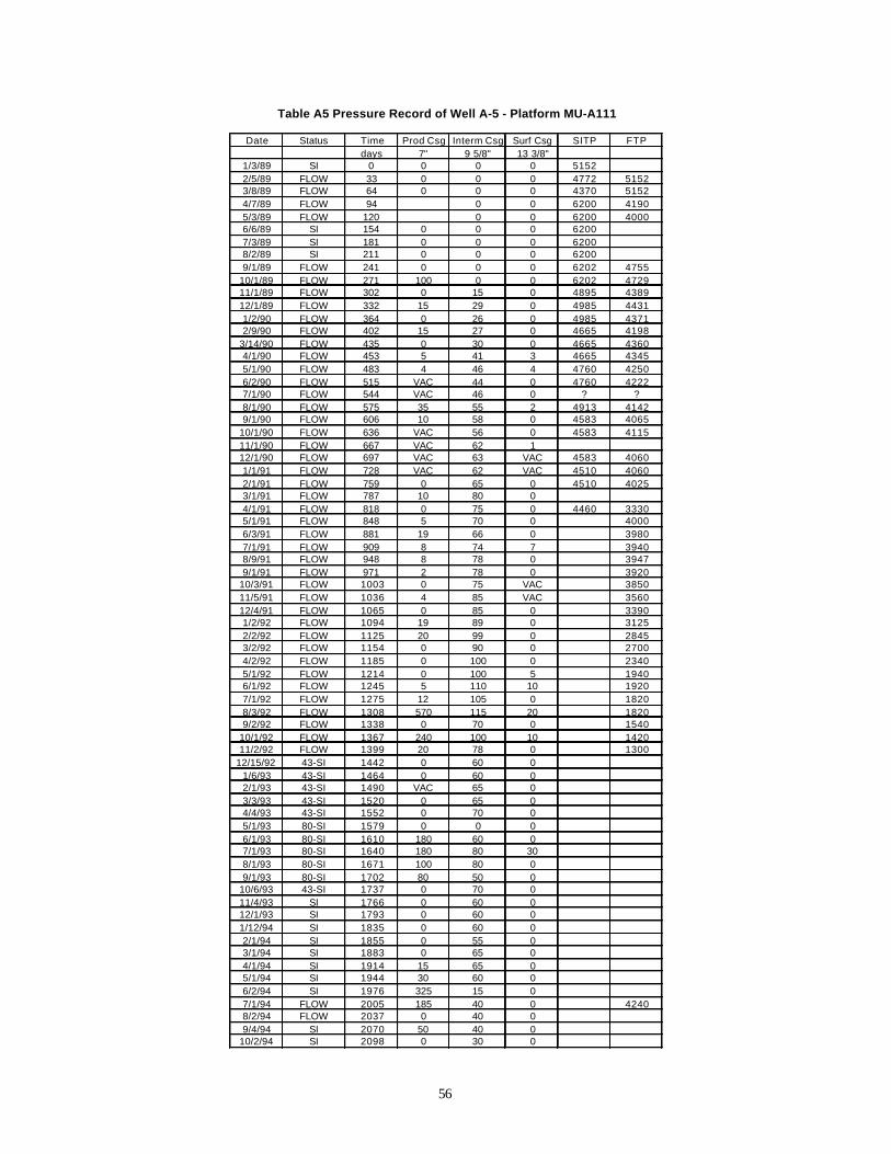
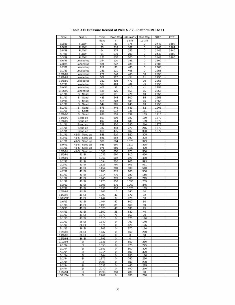
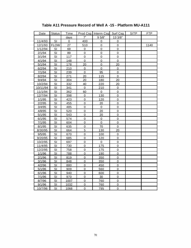
3.1 SCP Data BankAppendix A contains SCP data that were developed from field data. The data are made up ofcasing pressure records provided by various operators from 23 wells and are contained inMicrosoft Excel (.xls) files. Each file has a worksheet of raw data. Usually, charts include onlythe casing strings that have SCP problems, and chart names are the outer diameters of thosestrings. In some cases, if the string has more than one continuous buildup, each period has aseparate chart.
3.2 Statistical Analysis3.2.1 SCP OccurrenceWe analyzed casing pressure data from 26 wells. Among those, 22 wells, 85% of the total, haveSCP problems (Table 1). As indicated by the table, the following trends may be observed:• About 30.8% of the casing strings exhibiting SCP are production casing.
7
• About 65.4% of the casing strings exhibiting SCP are intermediate casing strings.• About 34.6% of the casing strings exhibiting SCP are surface casing strings.• About 15.4 % of the casing strings exhibiting SCP are conductor casing strings.
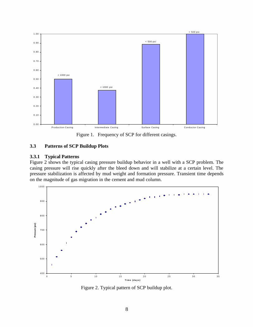
3.2.2 SCP Magnitude by Casing StringShown in Figure 1 is a cumulative frequency plot of the occurrence and magnitude of SCP in psiunits for the various types of casing strings. About 50 percent of the production casings and 35percent of the intermediate casings have SCP of less than 1000 psi. For the other casing strings,about 90 to 100 percent of the strings have SCP of less than 500 psi.
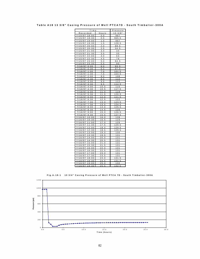
Table 1 - SCP OCCURRENCE IN VARIOUS CASING STRINGS
Count # Well # 6 5/8" 7" 7 5/8" 8 5/8" 9 5/8" 10 3/4" 11 3/4" 13 3/8" 16" 16" 20"1 MUA1 NA NA Y N2 MUA2 Y N Y Y3 MUA3 Y Y Y N4 MUA4 Y Y N N5 MUA5 Y Y N N6 MUA6 NA NA N N7 MUA7 N N N N8 MUA8 Y Y Y N9 MUA9 Y Y Y Y
10 MUA10 Y Y Y N11 MUA11 N N Y Y12 MUA12 Y Y Y N13 MUA13 N N N N14 MUA15 N Y N N15 MUA16 N N N N16 APTA19 NA Y NA NA17 APTA30 NA NA NA Y18 APTA31 NA Y NA NA19 APTL9 NA Y NA NA20 BPTB6 NA Y NA NA21 PTCA25C NA Y NA NA22 PTCA7D NA NA Y NA23 B7 N Y N N24 HIA1 N Y N25 HIA2 N Y N26 HIA3 N Y N
30.8 65.4 34.6Y- SCP problem; N- no SCP problem; NA - data not available.
8
0.00
0.10
0.20
0.30
0.40
0.50
0.60
0.70
0.80
0.90
1.00
Product ion Cas ing Intermediate Casing Surface Casing Conductor Cas ing
< 1000 psi
< 1000 psi
< 500 psi
< 500 psi
Figure 1. Frequency of SCP for different casings.
3.3 Patterns of SCP Buildup Plots
3.3.1 Typical PatternsFigure 2 shows the typical casing pressure buildup behavior in a well with a SCP problem. Thecasing pressure will rise quickly after the bleed down and will stabilize at a certain level. Thepressure stabilization is affected by mud weight and formation pressure. Transient time dependson the magnitude of gas migration in the cement and mud column.
4 0 0
5 0 0
6 0 0
7 0 0
8 0 0
9 0 0
1 0 0 0
0 5 1 0 1 5 2 0 2 5 3 0 3 5
T i m e ( d a y s )
Pre
ssu
re (
psi
)
Figure 2. Typical pattern of SCP buildup plot.
9
3.3.2 Anomalous PatternsFigure 3 shows an abnormal case of SCP response. The well was shut in at about 500 days. Thecasing pressure fluctuated significantly in response to frequent bleeding off of the wellheadpressure. Pressure monitoring was not frequent enough to show the pattern of pressure buildups.On the other hand, bleed-downs were too frequent, so a full pattern of pressure recovery did notdevelop. The plots do give a clue to the point at which the pressure would stabilize. Discerningbuildup patterns from this plot would be very difficult.
Figure 4. Undeveloped patterns of pressure build-up due frequent bleed-downs.
10
4. ANALYSIS OF SCP PRESSURE TESTING MECHANISMIn the Outer Continental Shelf (OCS) of GOM, weak marine formations contain pockets of over-pressured sand with gas or water. Intrusion of gas to the cement column may occur early, aftercement placement, or late, when the cement sheath is fully set. In the latter case, the migration ofgas is enabled by residual conductivity of the cemented annulus, as illustrated in Figure 5. Thisresidual conductivity may cause zonal isolation loss and failure of the cement to seal the annulus.Two physical mechanisms, matrix permeability and interfacial channeling, may contribute to thedevelopment of annular conductivity. Matrix permeability refers to flow within the body of thecement column. Interfacial channeling, on the other hand, refers to a micro-annulus between thecement column and the casing or rock.
Interfacial channeling is a mechanical discontinuity that forms a micro-annulus at thecontact surface of the cement column. At the cement-rock surface a micro-annulus could resultfrom poor removal of the mud cake. At the casing-cement contact, a micro-annulus is caused bythermal or hydraulic stresses after cement placement (pressure testing, completion fluidreplacement, stimulation treatment, wellbore cooling or heating). A very small micro-annulusmay provide a flow path for slow gas migration, resulting in SCP.
Mud
Gas Formation
Cement
Gas Bubble
Figure 5. SCP buildup mechanism.
After the cement is in place, the cement column may develop some secondary porosityand permeability. One mechanism of gas flow through the cement matrix is matrix channeling.After hydrostatic pressure in the cement slurry column drops below the value of the formationpore pressure, gas enters the slurry matrix either as a slug or dispersed fluid. The slug of gasmigrates upwards and creates a channel. Gas channels of up to about 1/4 inch in the cementmatrix have been documented in experiments. It seems unlikely, however, that such channelsmay provide flow paths for SCP. Their conductivity is too large to explain the small rate of SCPbuildup.
Another mechanism of gas flow through cement relates to the development of secondarypermeability in the cement matrix. The mechanism can be explained as follows: After the
11
hydrostatic pressure decrease to the formation pressure, cement hydration causes an absolutevolume reduction of the cement matrix. Chemical shrinkage is responsible for the creation ofsecondary porosity. Interstitial water in the cement matrix is trapped in the pores by capillaryforces. The trapped water is consumed in the hydration reaction, thus creating a void that resultsin pore pressure reduction and a “suction effect.” When combined with pressure underbalance,the suction effect may become a major mechanism for developing matrix permeability to gas.
The suction effect has been observed and described by several researchers (Levine etal.,1979; Tinsley et al., 1979; and Appleby, et. al, 1996). Laboratory measurements have shownthat a well-cured cement typically has a permeability on the order of 0.001 md, with a pore sizebelow 2 µ and a porosity around 35%. However, when gas is allowed to migrate within the slurrybefore complete curing, the pore structure is partially destroyed and gas generates a network oftubular pores that can reach 0.1 mm in diameter and lead to permeability as high as 1 to 5 md(Schlumberger, 1989). Matrix permeability is another likely mechanism of gas flow causingSCP.
Two possible configurations of the cement column in the annulus are common: cementtop extending to the surface or a mud column above it. In wells cemented to the surface, gasmigration can be considered a one-dimensional flow through a medium having someconductivity (Nishikawa, 1999). After bleed-down at a constant rate, the casing pressure increaseis analogous to the pressure transient buildup, as shown in Figure 6. The buildup behavior iscontrolled by cement properties, such as permeability and porosity, and by gas formationpressure.
Pressure
Time
Bleed off Bleed off
Figure 6. Conceptual patterns of consecutive SCP buildups.
If a mud column extends above the cement column, gas migration occurs in two stages.In the cement column, the gas flow follows Darcy’s Law; while in the mud column, gas bubblesrise through stagnant non-Newtonian drilling fluids. Not only will the gas migration be affectedby the characteristics of the mud, such as mud compressibility and density, but it will also beaffected by the top gas cap at the wellhead where migrating gas accumulates. We believe that thePVT behavior in this gas cap can be explained by the Real Gas Law. Therefore, the lower themud compressibility, the faster the gas bubbles rise, and the faster the pressure increases.Eventually, if not bled off, pressure at the wellhead would stabilize at a value equal to the gasformation pressure.
12
5. MATHEMETICAL MODELS OF SCP BUILDUP
5.1 Analytical Model of SCP Transient in Annulus Cemented to SurfaceIn this model, we assumed that the cement top is at the surface (Nishikawa, 1999). A diagram ofgas migration in a cement column is shown in Figure 7. To develop a mathematical model of gasmigration, the following assumptions were made:
Gas Zone
Well Head
Cement Column
Figure 7. Gas migration in an annulus cemented to the surface.
• The gas formation pressure is constant, because permeability of the gas zone is much higherthan that of the cement column.
• The pseudo gas pressure concept is used.• At the end of bleed down, gas is vented out from the well at a small constant rate.• The well is cemented to the surface.
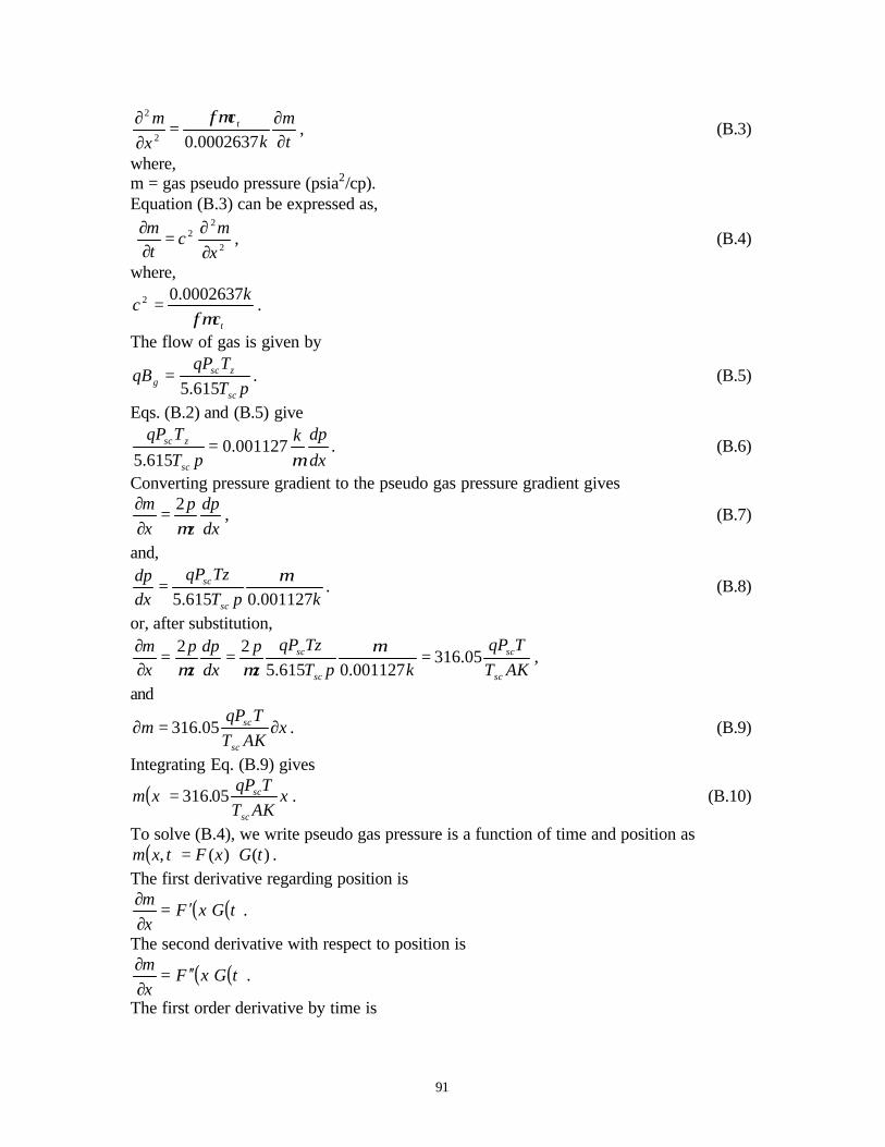
The flow of gas in the cement is described by the equation,
tm
k
c
xm t
∂∂=
∂∂
0002637.02
2 φµ(1)
where,k = average (equivalent) permeability of the annulusµ = viscosity of gasm = gas pseudo pressureN = cement porosityt = timex = vertical distance from bottom
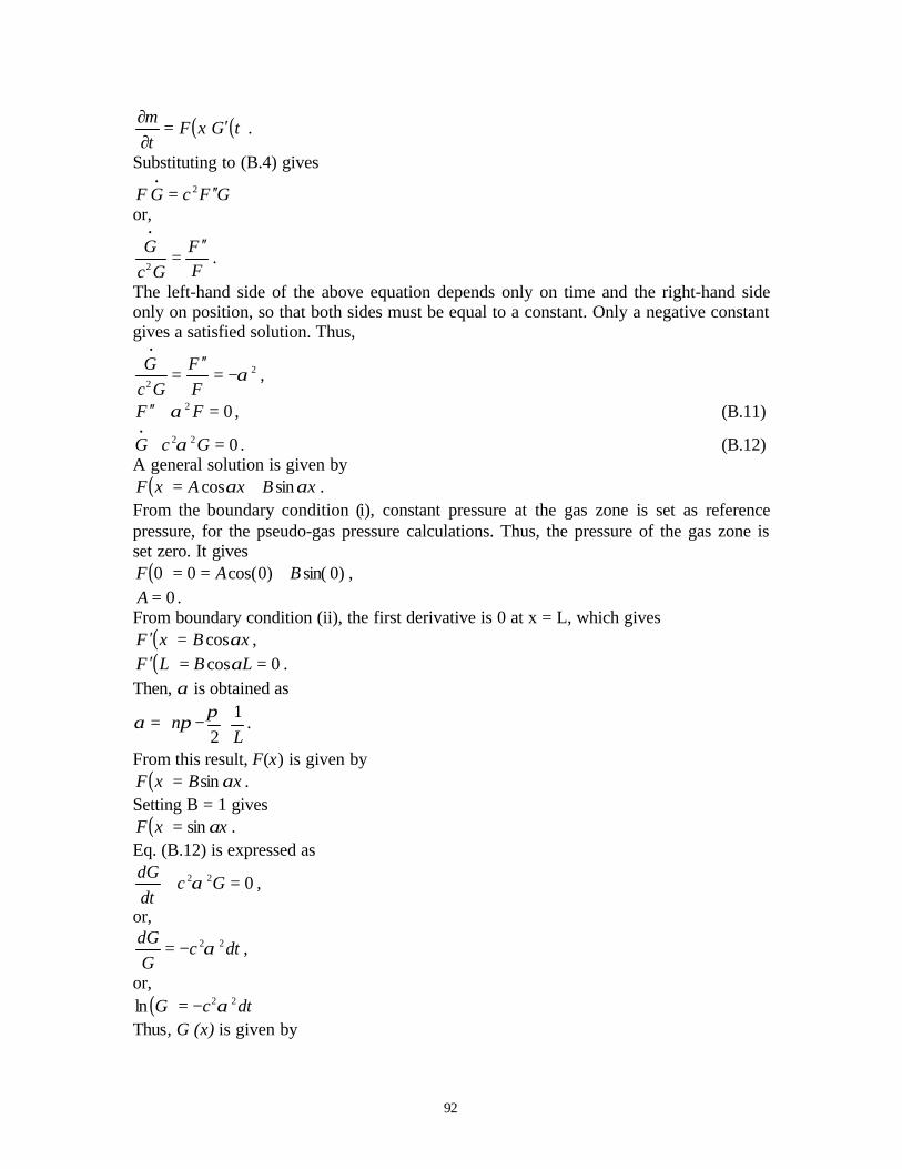
The solution to the flow equation is presented in Appendix B, and the analytical model is,
( ) ( ) tc
n
n
sc
sce e
AKT
TqP
LPmtm
22
12
1105.316)( α
α−
∞
=
+
⋅−−= ∑ . (2)
13
5.2 Numerical Model of SCP Buildup in Cemented Annulus with Mud ColumnIn this model, we assumed that a column of mud is above the cement top (Xu and Wojtanowicz,2001). Gas migration in the cement and mud columns is shown in Figure 8.
Lf
Lc
LtGas cap
Gas-cutmud
.const=ρ
Gas flowin cement
P = constantf
Pc(t)
Pt(t)
Figure 8. Conceptual diagram of SCP buildup in a cemented annulus with a mud column.
The following assumptions have been made in the derivation of this model:• Formation pressure does not change, i.e., constp f = .
• There is a steady-state flow of gas through the cement ( cLz ≤<0 ) at each time step in
response to changing pressure at the cement top, cp .• Gas density is neglected in the cement column.• The gas law deviation factor does not change, i.e., Z = constant.• The gas cut mud column is compressible.• Temperatures on top of the cement and mud ( wbT and whT ) are different.• Mud density is known and constant throughout the process, a pressure-averaged density of
the gas-cut mud.• The rising velocity of bubbles sgv is constant, and it controls the time step.
Based on those assumptions, we derived an iterative procedure for step-by-step calculation ofpressure buildup that is shown in detail in Appendix C. In the procedure, at the nth time step,pressure at the wellhead, tp , is
14
∆
+
−+−= −
=−
−−
−
−−
∑wb
nmm
n
k
kc
kcwh
nmm
ntn
tnmm
ntn
tnt TVc
tqpT
VcV
pVc
Vpp 1
1
2
1
11
1
11
4
21
(3)
and, pressure at the top of the cement column, cp , is
1'
111 052.0052.0 −
−−− ++= n
twh
ntn
mnt
nc L
TZR
MpLpp
fρ (4)
All symbols used in these formulas are defined in Appendix C.
6. EFFECT OF WELL PARAMETERS ON CASINGHEAD PRESSURE BUILDUP
6.1 Wellhead Pressure Transient Behavior in a Fully Cemented AnnulusFor wells cemented to the surface pressure transient is the mechanism of SCP buildup describedby the analytical model in Section 5.1. The top of the well is shut in after being open toatmospheric pressure. Pressure buildup follows and its pattern is controlled by conductivity ofannulus (in the model, cement permeability). Other parameters such as porosity, temperature andgas specific gravity may also play a role.
Effect of Cement PorosityInput data are shown in Table 2. Casing pressure buildups are shown in Figure 9. The resultsindicate that the effects of cement porosity variations are small, of the order of 10 percentpressure value.
Table 2. Input Data for Fully Cemented Well Study
Outer CSG ID & OH Size (in) = 19
Inner CSG OD (in) = 13.375
CMT Permeability (md) = 1
Porosity = 0.25-0.35
CMT column Length (ft) = 4000
Viscosity (cp) = 0.02
Reservoir Pressure (psi) = 2300
Total Compressibility psi-1 = 0.0003
Psc (psia) = 14.7
Tsc (°F) = 60
Temperature @ TOC (°F) = 90-110
Temperature @ BOC (°F) = 130
Flow Rate (scf/day)
= 0.010
Gas SG = 0.7-0.9
15
0
200
400
600
800
1000
1200
1400
0 100 200 300 400 500 600 700 800 900 1000
Time (days)
CasingP ressure(psia)
Porosity = 0.25Porosity = 0.30Porosity = 0.35
Figure 9. Effect of cement porosity on casing head pressure buildup.
Effect of TemperatureThe input data are shown in Table 2. Casing pressure buildups are shown in Figure 10. Theresults indicate that the temperature effect is small; increased temperature would give smallerpressure buildup.
0
100
200
300
400
500
600
700
800
900
1000
1100
1200
0 100 200 300 400 500 600 700 800 900 1000
Time (days)
CasingPressure(psia)
T = 90 degF
T = 100 degF
T = 110 degF
Figure 10. Effect of temperature on casing head pressure buildup.
16
Effect of Gas Specific GravityThe input data are shown in Table 2. Casing pressure buildups are shown in Figure 11. Again,the effect of gas gravity is insignificant.
0
200
400
600
800
1000
1200
0 100 200 300 400 500 600 700 800 900 1000
Time (days)
CasingPressure(psia)
SG = 0.7
SG = 0.8
SG = 0.9
Figure 11. Effect of gas gravity on casing head pressure buildup.
6.2 Pressure Buildup in Cemented Annulus with Mud ColumnWhen a column of mud sits on top of the cement, the mechanism of pressure buildup is differentthan that for fully-cemented well and described by the numerical model in Section 5.2. After theannulus is shut-in, initial pressure at the cement top is high and controlled by hydrostaticpressure of the mud column. Thus, the initial pressure drawdown across the cement column ismuch smaller than that in the case of a fully cemented well. Also, during the process of gas flow,a gas cap at the casing head is formed and controls the gas flow and pressure buildup. Thus, newparameters should be added to the list of factors controlling the process: mud characteristics inaddition to cement and formation properties.
Effect of Gas Cut CapHere, the cap represents the void between the top of the mud column and the well head. Usually,this cap is filled with gas or gas-cut mud with a high gas concentration. In our study, we foundthis cap functions as a “stabilizer.” The larger the gap, the slower the casing pressure will reachto the stable pressure (See Figure 12).
Effect of Mud CompressibilityIn this model, we also considered mud compressibility. Figure 13 shows the effect ofcompressibility very clearly. The higher the compressibility, the slower the casing pressurebuildup.
0
500
1000
1500
2000
2500
0 5000
10000
15000
20000
25000
30000
Time(mins)
1.5e-3
1.5e-6
1.5e-4
Figure 13. Effect of mud compressibility.
Effect of Cement PermeabilityIn this model, we assume that conductivity of the cemented section of the annulus, whethercaused by micro-channeling or matrix permeability, is represented by a “cement permeability”property. The effect of cement permeability is opposite to that of the mud compressibility, i.e.,the more permeable the cement, the faster the casing pressure increases (See Figure 14).
18
0
500
1000
1500
2000
2500
0 10 20 30 40 50 60 70 80 90
Time (month)
Cas
ing
Pre
ssu
re (
psi
)
Km = 0.001
Km = 0.0005
Km = 0.005
Field Data
Figure 14. Effect of cement permeability.
Effect of Formation PressureIn the model, the formation pressure is assumed constant throughout the whole process ofpressure buildup. Its magnitude will affect the equilibrium pressure at the casing head after along time. Obviously, the higher the formation pressure is, the higher the equilibrium pressureand the longer the need for pressure stabilization (See Figure 15).
0
500
1000
1500
2000
2500
3000
0 10 20 30 40 50 60 70
Time (month)
Cas
ing
Pre
ssu
re (
psi
)
Pf = 6500 psi
Pf = 6000 psi
Pf = 7000 psi
Field Data
Figure 15. Effect of formation pressure.
Effect of Gas Slip Velocity in MudAs shown in MMS statistics, most SCP problems happened in the intermediate casing where themud column in the casing is relatively short compared to the whole length of the casing, so thetravel time of the gas across the mud column to the wellhead is relatively short. Furthermore,
19
according to some studies, gas will rise faster in viscous mud than in water because of the size ofthe equilibrium slug (A. B. Johnson, et al). Therefore, we simplified the model by assuming thatthe gas travel time in the mud is in the range of the time step used in the model, which meansthat all the gas generated at the cement top is transferred to the gas cap in one step.
7. METHOD FOR SCP DIAGNOSISBased upon the theory and numerical model presented above, we have developed a method,software, and procedure for analyzing casing head pressures qualified as SCP. Qualification isnot part of the method since, by the MMS definition, this method has been based uponrecurrence and source of pressure buildup rather than the pattern of pressure behavior in time.The diagnostic method enables determination of well parameters that control SCP but are usuallyunknown, such as severe channeling in the cement, depth of the pressure source formation, andgas pressure gradient.
7.1 Validation of Numerical Model with Field DataMatching the field and theoretical data allows the numerical model to be used to determine thetwo most uncertain parameters affecting SCP: the formation pressure and cementing quality. Thematched data are shown in Table 3.
Table 3. Results of Matching Field Data
Case I Case IIk md 0.001* 0.0028*
Twb R 575 552T R 630 584
Twh R 520 520D1 ft 0.829 0.829D2 ft 0.583 0.635Lc ft 1821 2783
7.1.1 Case 1: Partial SCP Buildup DataA schematic of gas production Well A is shown in Fig. 16. The well is located offshore in GOM.SCP has developed in the annulus of the 103/4-inch intermediate casing of the well. Casing headpressure rose from 200 psi to 1600 psi and was still increasing after 9 months of buildup, asshown in Fig. 17.
20
Drive Casing26”738’
Conductor Casing
Surface Casing16” 65# H-40 STC1332’
Intermediate Casing10 3/4” 45.5# K-55 STC4310’
11196’
Production Casing7” 29# 55# N-80 LTC
Figure 16. Schematic of Well A, offshore GOM.
Using the numerical model, we matched the pressure data and found out that the casingpressure would stabilize at about 2200 psi in 30 months, as also shown in Fig. 17. In this case,the operator was not sure about two sets of data: cement permeability and formation pressure.The matched value for permeability, 0.001md, was very small. However, laboratorymeasurements (discussed above) have shown similar values for well-cured cements. Therefore,the matched cement permeability was realistic to some degree.
Casing Pressure Match
0
500
1000
1500
2000
2500
0 20 40 60 80 100 120 140
Time (month)
Cas
ing
Pre
ssu
re (
psi
)
TheoreticalActual
Figure 17. SCP buildup match and extrapolation for Well A.
21
The formation pressure controls the stabilized value that the buildup pressure can reach.Only for pressures around 6500 psi can the top casing pressure reach 1600 psi in 9 months. Inthis case, the method helped the operator to determine formation pressure and cementing quality.
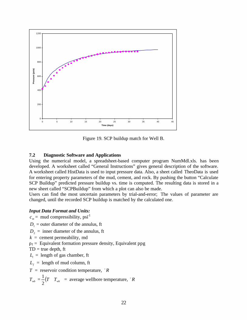
7.1.2 Case 2: Complete SCP Buildup DataIn Case 2, Well B, shown in Fig. 18, exhibited SCP in the intermediate casing. Before the casingpressure buildup, shown in Fig. 19, was recorded, the well had been frequently bled down. Aftereach bleed-down, heavier mud would be pumped into the 103/4-inch intermediate casing annulus.The operator would record the volume and weight of the bled and pumped muds. After onemonth of buildup, the casing pressure stabilized at about 1000 psia.
D r i v e P i p e
2 6 ”5 8 2 ’
C o n d u c t o r C a s i n g
2 0 ” 9 4 # H-40
Surface Casing16” 75# K-554776’
Intermediate Casing10 3/4” 45.5# L-806433’
9084’
Production Casing7 5/8” 33# N-80
1061’
Figure 18. Schematic of Well B, offshore GOM.
The pressure match in Figure 19 is not as perfect as in the previous case due to the followingreasons: First, it was very difficult to estimate mud density due to frequent bleed-downs and lackof original mud density records. (We assumed that the mud in the annulus should be heavier thanthe bled out mud in the last bleed down.) Secondly, no data on mud compressibility wasavailable. In this case, the method helped the operator to determine the degree of channeling inthe cemented annulus. (The matched cement permeability was 0.0028md.) Interestingly, the gasformation pressure gradient (at the 103/4-in. casing shoe) was found to be normal, 0.46 psi/ft.
22
0
200
400
600
800
1000
1200
0 5 10 15 20 25 30 35 40 45
Time (days)
Pre
ssu
re (
psi
a)
Figure 19. SCP buildup match for Well B.
7.2 Diagnostic Software and ApplicationsUsing the numerical model, a spreadsheet-based computer program NumMdl.xls. has beendeveloped. A worksheet called “General Instructions” gives general description of the software.A worksheet called HistData is used to input pressure data. Also, a sheet called TheoData is usedfor entering property parameters of the mud, cement, and rock. By pushing the button “CalculateSCP Buildup” predicted pressure buildup vs. time is computed. The resulting data is stored in anew sheet called “SCPBuildup” from which a plot can also be made.Users can find the most uncertain parameters by trial-and-error; The values of parameter arechanged, until the recorded SCP buildup is matched by the calculated one.
Input Data Format and Units:
mc = mud compressibility, psi-1
1D = outer diameter of the annulus, ft
2D = inner diameter of the annulus, ftk = cement permeability, mdρf = Equivalent formation pressure density, Equivalent ppgTD = true depth, ft
Matching Hints:Two strings of SCP buildup data, Pt, recorded and calculated is stored in the sheet called“SCPBuildup”. Also the difference between the data is listed in the sheet. Pushing the “OK”button in the message box, gives a comparison plot of the two pressure buildups. The plot isstored in the sheet, “MatchingPlot”. By visually inspecting the plot a user can assess quality ofthe match. If the match is poor, the user would change input data in the “TheoData” sheet, runthe program again, and repeat the procedure until satisfactory match is achieved.The following are hints on how to change input data:
• If the calculated value of stabilized Pt is too high, the assumed value of the formationpressure equivalent density, ρf , may be too large, or the formation is shallower thanassumed. Therefore, one of the two parameters (the most uncertain one), pore pressure ordepth, should be decreased within acceptable limits.
• If Pt increases faster than the actual data, cement conductivity k should be reduced (or,mud compressibility mc increased) step-wise until a matching trend is obtained.
8. SCP DIAGNOSIS: CONCLUSIONS AND RECOMMENDATIONS
Conclusions:• Statistical analysis of casing pressure in a single oilfield shows similar trends to those
reported by MMS for the whole GOM. Thus, we conclude that the SCP problem iswidespread and independent from conditions of specific oilfield in the GOM. Also, theanalysis method validated for one oilfield should work anywhere in the GOM.
• SCP buildup pattern is controlled by parameters of cement, mud and gas invasion zone.Using the mathematical model, we theoretically analyzed the effects of those parameters andfound out as follows:
24
− Large casing gas cap prolongs the SCP buildup cycle and would complicate buildupanalysis by reducing the buildup plot resolution. Operators should keep this cap as smallas possible by filling up the well after the bleed-off.
− Mud compressibility controls the early stage of SCP buildup. Thin drilling mud havinglow tendency for gas cutting would considerably improve the analysis of SCP buildup byremoving the compressibility effect.
− Cement permeability parameter represents the quality of cementing. It controls early stageof SCP buildup. Thus, SCP buildup rate analysis may become an overall measure of theannular seal performance of the well.
− Formation pressure controls the maximum value of stabilized SCP, with high formationpressure resulting in high stabilized SCP value. Potentially, a combined analysis of thestabilized SCP value, mud density, top cement depth and formation pressure gradientsmay identify the gas invasion zone. In case when maximum value of SCP is not attainable(too high) from the field data, the mathematical model presented here could extrapolatethe value.
• Field validation of the model, presented here, gives acceptable estimates of the gas-sourceformation pressure, cement conductivity, and expected maximum casing pressure value.Ambiguity of the analysis can be significantly reduced by reducing the number of unknownparameters to two: cement conductivity and formation pressure. Early stage of SCP buildupis controlled by cement conductivity; while stabilized pressure is determined by formationpressure. If data collected could exclude the effects of other parameters, the test analysiswould be very straightforward.
• The model has been simplified by disregarding effects of gas migration in the mud and gascutting of the mud. The two parameters may have strong effects on the rate of SCP buildup.Future study should address SCP buildup analysis including the effect of gas migration innon-Newtonian fluids.
• Measuring the bleed rate is as important as the pressure record when determining thepotential hazard posed by sustained casing pressure.
• Gas flow through the unset cement matrix seems to be a major cause of sustained casingpressure; the matched values of cement permeability support this conclusion.
• The analytical model provided a basic analysis of specific SCP buildup in an annuluscemented to the surface.
• The numerical model seems more feasible for prediction and diagnosis of casing pressurebuildup behavior because it considers the effect of a mud column above the cement.
• There are two major limitations of this study: mathematical modeling was simplified; and, notesting procedure combining bleed-down and buildup pressures was developed.
• Recommendations:In addition to pressure and flow rate records, annular mud, cement, and formation information iscritical for proper diagnosis of SCP. Also, the configurations of each well, such as cement depthand fluid (mud) level, are important for obtaining a good match. Therefore, sampling andmonitoring procedures should be modified in the future.
In view of this work, we recommend continuing this research program to develop criteriafor the SCP risk evaluation. As stated above, flow rates of gas and liquids causing the SCPshould be included in the risk evaluation procedures. In the procedure, the affected annuli shouldbe produced (or vented out) under controlled conditions. The venting rate should be measured
25
and controlled by a choke smaller than 1/8 inch. Also, the well should be regularly shut-in andtested for ability to rebuild the casing pressure. Also, there is a need for supporting the modifiedcriteria with engineering science.
Additional research should be conducted to develop improved diagnostic test proceduresfor wells with SCP. The main objective of such research would be to provide theoretical supportfor the criteria, standards, and procedures to be used in identifying wells with SCP, assessing theseverity of the problem, and defining the level of tolerance to the problem. Also, the programshould develop field-deployable procedures for multi-rate testing that would include the bleed-down and buildup procedure and analysis method.
9. CURRENT STATUS OF SCP REMOVAL: CYCLIC INJECTIONIn the recent review of SCP problems, Bourgoyne, et al. (Bourgoyne, 2000) discusses variousmethods, both with and without using a drilling rig, of SCP removal. In principle, the rig-lessmethods involve injecting high-density fluid into the affected annulus in order to kill SCP. Thefluid is injected either at the surface directly into the casing head (Bleed-and-Lube method) orthrough a flexible tubing inserted to a certain depth in the annulus (Casing Annulus RemediationSystem, CARS). The concept of these two methods is to replace the gas and liquids producedduring the pressure bleed-off process with high-density brine, such as Zinc Bromide. The goal ofthese techniques is to gradually increase the hydrostatic pressure in the annulus.
The lube-and-bleed procedure involves bleeding small amounts of lightweight mixtures ofgas and fluid from the annulus and lubricating in Zinc Bromide brine over several treatmentcycles. A limited number of case histories reported the lube-and-bleed method as partiallysuccessful. In one of these cases, SCP in the 13-3/8”casing was reduced from 4,500 psi to 3,000psi. The operation took over a year with numerous cyclic injections, during which 118 bbls of19.2 ppg Zinc Bromide brine replaced 152 bbls of the annular fluid (a gas-cut water-based mudhaving density of 7.4-9.5 ppg) (Hamrick and Landry, 1996).
Other operators also observed incomplete reduction in surface casing pressures after usingthis method. In one field application the brine was pumped into the SCP affected wells throughthe casing valves on top of the closed-ended annuli, and the operator estimated that the volumesthat could be pumped (or lubricated) during a given cycle were as small as a quart per one cycle.On the other hand, the required volume of heavy fluid necessary to overbalance the casingpressure was usually from as low as 5 barrels to as high as 80 barrels. Thus, completion of thejob would have required months, or years, of application. Additionally, surface pump pressureswould reach relatively high levels. In some cases, several iterations of pressuring up to highlevels and bleeding off (or pressure “cycling”) has been proven to worsen the casing pressureproblem, probably due to opening a micro-annulus in the cement or breaking down previouslycompetent cement.
Field observations indicate that pressures can increase while applying this method(Bourgoyne et al., 2000). The hypothesis has been proposed that this occurs when a new “gasbubble” migrates to the surface. After trying the lube-and-bleed method for several years inseveral wells, the field results have not been as promising as first indicated.
The CARS system is similar to the lube-and-bleed process in that it is designed to placeheavy fluids into the casing annulus without using a workover rig or perforating. The fluids areintroduced by inserting a small diameter flexible hose into the casing annulus through the casingvalve. After placing the hose at a certain depth, heavy fluids can be circulated through the hose,
26
as opposed to the lube-and-bleed process, in which fluids are squeezed into the closed annulussystem from the top of the annulus.
Although the CARS system has been used successfully in many wells and the CARSequipment functioned satisfactorily during the jobs, it is still too early to make conclusions as tothe effectiveness of using the system to satisfy MMS regulations. To date, field experience withCARS showed that the maximum injection depth could not exceed 1000 feet, while in most wellsthe injection depth was less than 300 feet and could not be increased. Thus, injection depth hasbecome one of the major barriers for widespread use of CARS.
10. EXPERIMENTAL ASSESSMENT OF CYCLIC INJECTIONGiven the depth limitation of CARS, the two methods (Bleed-and-Lube, and CARS) wouldrequire multi-cyclic injection of heavy liquid to kill SCP in the affected annulus. The objective ofthis study was to evaluate the performance of cyclic injection in view of the efficiency ofdisplacing annular fluid with injected fluid (Nishikawa,1999; Nishikawa, Wojtanowicz andSmith, 2001)
Several factors may affect displacement efficiency. For example, a small clearance in theannulus would restrict a downward movement of the injected (kill) liquid. Using brine as a killliquid brings about a miscibility problem. High miscibility would not contribute to weighting upthe fluid in the whole annulus, only in the top sections. Thus, cyclic injection may not beeffective for killing SCP because most of the injected fluid would return when bled off.
In this work, we identified and studied several mechanisms of displacement in the cyclic-injection process. Using a pilot-scale physical model of annulus and brine (CaCl2) as a primarykill liquid, we investigated efficiencies of cyclic injection for different rheology and miscibility.An annular fluid containing gas was not considered in this study.
10.1 Experimental Design
10.1.1 Physical ModelTo investigate the cyclic-injection method, a physical model of casing annulus was designed andfabricated as shown in Fig. 20. A 3-in. clear PVC (ID 3 in./OD 3.5 in.) pipe was installed insidea 6-in. clear PVC pipe (ID 6 3/8 in./6 5/8 in. OD) to construct the annulus. This 3-in. pipe wasopened at both ends and welded to a 6-in. plastic flange. A 3/8-in. inlet was installed on the 6-in.flange to pump a kill liquid into the annulus. At the top of the 6-in. pipe, a 3/4-in. outlet wasinstalled just below the flange, and a 3/4-in. valve was attached to this outlet. This valverepresented a needle valve used in field operations. At the bottom of the apparatus, a 3/4-in.outlet with two valves was installed. A pressure gauge was installed between the valves tosimulate the location of the cement top in the annulus.
27
In field operations, after a needle valve is installed, a kill liquid is injected (“Injection” inFig. 21). Then the system of the annulus is shut-in (“shut-in” in Fig. 21). After a certain time ofshut-in to settle the kill liquid, the needle valve is opened again. The kill liquid returns mixedwith the annular fluid through the needle valve, because a compressed annular fluid flowsbackward to release the injection pressure.
This operation would be difficult to simulate experimentally by designing an apparatusbecause of the high working pressure. However, to investigate cyclic injection, an experiment
Figure 20. Physical model of a well annulus.
10 ft of 6” Pipe
10 ft of3” Pipe
3/4” Outlet
PressureGauge
3/8”
inlet
3/4” outlet
6.25
Mud Mixer
Samplemud
SampleMud
0.75 ft
Pump
28
must simulate only the cyclic procedure of injection, shut-in, and bleed-off at any pressure. It isconceivable that if the method worked at low pressure, it would also work at high pressure.
Figure 21. Cyclic injection procedure.
Mud
Gas Formation
Cement
GasBubble
Injection
Mud
Gas Formation
Cement
GasBubble Mud
Gas Formation
Cement
GasBubble
Injection Shut-In Bleed-Off
Figure 22. Simulation of a single injection cycle in experiments.
KillLiquidInlet
The TopValve
InitialFluidLevel
6 3/8”-3 1/2”Annulus
3”Pipe
FluidLevel of3” Pipe
Step1 Step 2 Step 3
29
To simulate killing SCP, we applied a U-tube effect instead of fluid compressibility in theannulus (Fig. 21 and Fig. 22). Initially, fluid levels were the same between the 6 3/8-in. and 31/2-in. annulus and the 3-in. pipe (Condition 1 shown in Fig. 22). The kill liquid was injectedinto the annulus through the top flange with a closed position of the top valve (Condition 2shown in Fig. 22). The top valve represented a needle valve for field operations. The liquid levelincreased inside the 3-in. plastic pipe in response to the volume of the injected kill liquid(Condition 2 in Fig. 22). When the top valve was opened, the fluid returned from the top outlet tokeep the balance of hydrostatic pressure (Condition 3 shown in Fig. 22). If the annular densitywere not changed, the fluid levels would be equal. If the annular density increased, a fluid levelin the 3-in. pipe would be higher than the level in the annulus.
The capacity of the apparatus is shown in Fig. 23. The annular volume was 10.2 gal.; the3-in pipe volume was 3.3 gal. There was 1.7 gal below the 3-in. pipe. Thus, an injected volumein one cycle was below 1.7 gal in all the experiments.
10.1.2 Data Analysis MethodTo evaluate the performance of cyclic injection, a method was developed based upon thefollowing concepts: Typically, an annular fluid above the top of the cement is a Bingham Plasticfluid with some gas content. In this study, we considered combinations of the annular fluid withvarious types of displacement liquids, such as Newtonian-miscible fluid (brine), Bingham-miscible fluid (drilling mud), and Newtonian-immiscible fluid (oil base mud). In addition to fluid
Pressure Gauge
Capacity of 3” Pipe = 3.3 gal
Sump volumebelow 3” Pipe= 1.7 gal
Annular capacity: 6” pipe (6.625” OD, 6.375” ID)and 3” pipe (OD 3.5”, ID 3.0”),= 10.2 gal
Figure 23. Volumetric capacity of physical model.
30
properties, the following patterns of mixing and displacement were considered, as shown in Fig.24.
Case A: Kill liquid moves downwards and settles without mixing with the annular fluid.Case B: There is some liquid settling and mixing at the bottom of the annulus.Case C: Kill liquid mixes perfectly with the annular fluid.Case D: There is some mixing in the top section of annulus with little settling.Case F: Kill liquid stays at the wellhead on top of an annular fluid—no mixing, no
settling.When a mixed pattern was observed, we applied a two-letter category. For example, if a killliquid showed Case B at early time, followed by Case A, we recorded the kill fluid pattern asCase B-to-Case A.
Injectedliquid
Annularliquid
Inlet ofinjectio n
CasingValvejustclosed
Figure 24. Displacement performance patterns.
Partialuppermixing
Case D
Partiallowermixing
Case B
Perfect settling@
displacement
CASE A
No settling@
displacement
CASE E
Perfectmixing
CASE C
Bleed off Bleed off Bleed offBleed off Bleed off
Valvejustopened
31
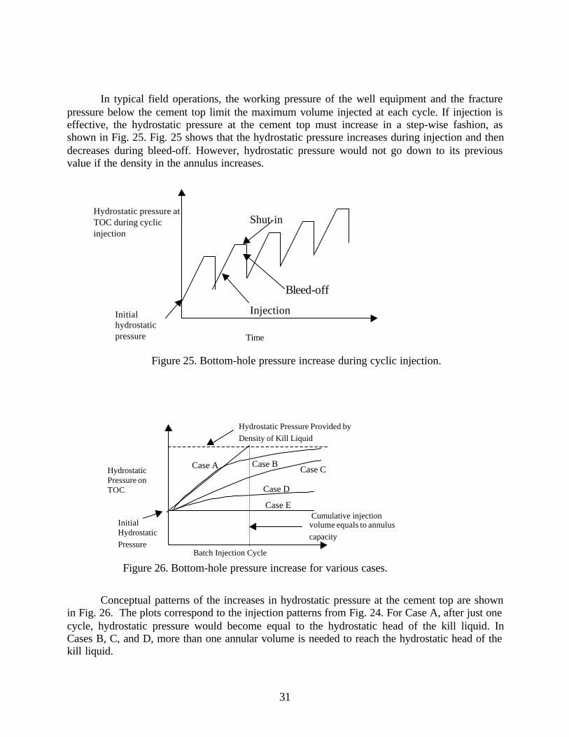
In typical field operations, the working pressure of the well equipment and the fracturepressure below the cement top limit the maximum volume injected at each cycle. If injection iseffective, the hydrostatic pressure at the cement top must increase in a step-wise fashion, asshown in Fig. 25. Fig. 25 shows that the hydrostatic pressure increases during injection and thendecreases during bleed-off. However, hydrostatic pressure would not go down to its previousvalue if the density in the annulus increases.
Conceptual patterns of the increases in hydrostatic pressure at the cement top are shownin Fig. 26. The plots correspond to the injection patterns from Fig. 24. For Case A, after just onecycle, hydrostatic pressure would become equal to the hydrostatic head of the kill liquid. InCases B, C, and D, more than one annular volume is needed to reach the hydrostatic head of thekill liquid.
Figure 25. Bottom-hole pressure increase during cyclic injection.
Shut-inHydrostatic pressure atTOC during cyclicinjection
Time
Injection
Bleed-off
Initialhydrostaticpressure
Figure 26. Bottom-hole pressure increase for various cases.Batch Injection Cycle
Case A Case B
Case D
Case E
HydrostaticPressure onTOC
Hydrostatic Pressure Provided byDensity of Kill Liquid
Cumulative injectionvolume equals to annuluscapacity
Case C
InitialHydrostaticPressure
32
Finally, we needed a criterion to evaluate the process quantitatively. We could predict thehydrostatic pressure for Cases A and E. However, we could not estimate how much pressurewould increase in other cases, except for Case C. For Case C, we developed a mathematicalmodel as follows:
The mixture density after one injection is
ko
kkoo
VVVV
++
=ρρ
ρ1 , (5)
where,ρo= initial density in the annulus (ppg),ρk = density of the kill liquid (ppg),ρ1 = density in the annulus for the first injection (ppg),Vo = initial annular volume (gal),Vk = one-cycle volume of the injecting kill liquid (gal).
If we inject the same volumes into the annulus several times, the mixing densities will increasein the following manner. The second injection, following Eq. (5), gives the annular density,
( ) ( )ko
kko
ko
kkoo
ko
kkoko
kkoo
VVV
VVV
VVVV
VVVV
VV
++
++
=+
+
++
=ρρρ
ρρρ
ρ 22 . (6)
The third injection gives
( ) ( )
( ) ( ) ( ) ( )
22
33
3
2
3
ko
kko
ko
kko
ko
kk
ko
oo
ko
kkoko
kko
ko
kkoo
VVV
VVV
VV
VV
V
VV
V
VV
VVVV
VV
VV
VV
++
++
++
+=
=+
+
++
++
=
ρρρρ
ρρρρ
ρ (7)
At n time injection, the density in the annulus gives
( ) ( ) ( ) ( ) ( )
+
+++
++
++
++
= −
−
−
−−
kon
ko
no
nko
no
nko
no
kknko
noo
n VVVV
V
VV
V
VV
VV
VV
V 12
3
1
21
LLρρ
ρ (8)
where,ρn = density in the annulus (ppg)
Substituting, [ko
o
VVV
r+
= ] gives,
( )rrrrrVV
r nnn
o
kko
nn +++++= −− 221 LL
ρρρ . (9)
Multiplying both sides by r gives,
( )2311 rrrrrVV
rr nnn
o
kko
nn +++++= ++ LL
ρρρ . (10)
33
Subtracting Eq. (9) from Eq. (10) gives,
( ) )1()1(1 n
o
kknon rr
VV
rrr −⋅+−=−ρ
ρρ
Thus, density after the nth injection cycle is,
rrr
V
Vr
n
o
kknon −
−⋅+=1
)1(ρρρ . (11)
For r < 1; 0lim =∞→
n
nr
koko
o
o
kk
o
kkn
o
kknonn VVV
V
V
V
rr
V
V
rrr
V
Vr ρ
ρρρρρ =
−+⋅=
−⋅=
−−⋅+=
∞→ 11)1(
lim (12)
knnρρ =
∞→lim (13)
where,
ko
o
VVV
r+
= ,
n = number of injection cycles.
Formula (13) implies that the density in the annulus approaches the density of the kill liquid for alarge number of injection cycles.
This mathematical model provides a criterion for evaluation of the experiments. As areference level, we used Case C in Fig. 24 as the “criterion of perfect mixing (CPM).” If, afterseveral injection cycles, hydrostatic pressure increased at a rate greater than that for Case C inFig. 24, we designated displacement performance as “good.” Otherwise, the performance wasdesignated as “poor.”
10.1.3 Selection of Displacing FluidsOne of the main purposes in this experimental research was to investigate brine as a kill liquid.This section presents a selection of brines.
Density RangeTable 4 shows the approximate density range of solid-free salt solutions. Potassium chloride
brines provide densities up to about 9.7 lb/gal at 85°F. Sodium chloride brines provide densitiesup to 9.8 lb/gal. Sodium-chloride/Calcium-chloride mixtures can provide densities from 10.0 to11.0 lb/gal. Calcium chloride can be used for weights up to 11.7 lb/gal. Formulations of calciumchloride and calcium bromide can provide solid-free densities up to 15.0 lb/gal. Use of ZincBromide can increase the solids-free fluid density up to 19.2 lb/gal.
Corrosiveness, Toxicity, and SafetyWhen mixing high concentrations of CaCl2, CaBr2, or ZnBr2, precautions should be taken tokeep the dry chemical dust out of the eyes and lungs. Rubber protective clothing should be wornto prevent skin damage. Considerable heat may be generated; thus, precautions should be takento prevent burns. CaCl2-CaBr2 brine toxicity is low enough to allow use of these solutions inmarine waters. ZnBr2 can be toxic to fish, which limits its use in offshore areas. Onshore,precaution must be taken to avoid contamination of water supplies. CaCl2-CaBr2 brines arealkaline, whereas ZnBr2 brines are slightly acidic and therefore more corrosive.
CostHeavy brines are expensive. 15.0-lb/gal CaCl2-CaBr2 brine costs about 25 times more than 10.0-lb/gal CaCl2 brine. Eighteen-lb/gal CaCl2-CaBr2-ZnBr2 brines cost over 80 times more than 10.0-lb/gal CaCl2 brine.
10.1.4 Testing ProcedureCombinations of all fluids considered for this study are shown in Table 5. Table 6 is the actualmatrix of our experiments. All results are shown in Appendix D.
Table 5. All Possible Combinations of Displacing and Annular FluidsCase Kill Liquid Annular Fluid Miscibility Remarks
*Data from Experiments 7 and 8 are not included in Appendix D
A testing procedure was designed to investigate the performance of each experimental runcompared to CPM. The procedure was as follows:1. Fill the annulus through the inside pipe up to the level of the top valve.2. Close the top valve and read pressure.3. Inject fixed volume of kill liquid and stop pumping.4. Record the value of a bottom pressure.5. Wait three to five minutes (shut-in).6. Take a minimum volume sample of a fluid from the bottom valve and measure a density
(rheology by Fann 35 viscometer, if necessary).7. Open the top valve to bleed off the pressure.8. Record value of the bottom pressure.9. Take a sample from the top valve and measure its density (rheology by Fann 35 Viscometer,
if necessary).10. Close the top valve.11. Repeat steps 3 to 8 until there is no significant change of the bottom pressure.
10.2 Results and Analysis
10.2.1 Miscible Displacement Experiments
Brine (CaCl2) into WaterFirst, we conducted an experiment using a single-cycle injection of brine (CaCl2) into water. The11.0-ppg brine (CaCl2) was pumped into the annulus until a total volume of 1.6 gal was reached.We stopped pumping at 7 min. We sampled the fluid from the bottom valve and recorded thedensity every minute for 10 min. After 60 min, we bled off and sampled from both the bottomand top valves. The result is shown in Experiment 1 of Appendix D and Fig. 27.
Second, we conducted Experiment 2 using multi-cyclic injections. We injected 1.4 gal of11-ppg brine (CaCl2) into an annulus filled with water, then shut-in 3 minutes, and bled-off. Werepeated this procedure 9 times. The results are shown in Fig. 28 and Appendix D. The resultsshow that the hydrostatic pressure increases with injections, and the same density comes fromthe top and bottom in every injection. However, we did not see a stabilized hydrostatic pressureby the kill liquid.
Finally, we conducted Experiment 3 to find out the final condition that the hydrostaticpressure achieved with this kill liquid, as shown in Fig. 30. We injected 11.3 ppg brine (CaCl2)into an annulus filled with 10.3 ppg brine (CaCl2). The injections were repeated until thehydrostatic pressure stabilized. It took 18 cycles to reach the maximum pressure with the 11.3-
36
ppg brine. In addition, every sample from the top and bottom valves indicated the same density,as shown in Fig. 31.
Results from Experiment 1 showed the density increasing with pumping up to a value of8.69 ppg. This density matches the density calculated by Eq. (5.1). Moreover, the densities fromthe top valve and that of the bottom valve were the same when we sampled them 60 minutesafter the injections started. Thus, this single-cycle injection was evaluated as CPM.
In addition, we compared Experiment 2 with the calculated values from Eq. (11). Thecomparison is shown in Fig. 32. The results matched CPM. We also compared a calculation fromEq. (11) with results from Experiment 3, as shown in Fig. 33.
From these comparisons, we concluded that the cyclic injection of brine into an annulusfilled with water could be classified as CPM (Case C shown in Fig. 24). In other words, thiscombination will work in the field. If we inject a large amount of the kill liquid, we will reach adesirable hydrostatic pressure eventually.
8.308.358.408.458.508.558.608.658.708.75
0 2 4 6 8 10
Time (min), Total 1.6 gal Injected
Den
sity
at B
ott
om
(psi
)
Density after 60 min from top and bottom
Stop pumping
Start pumping
Figure 27. Results of Experiment 1.
4.5
5
5.5
6
6.5
7
7.5
0 20 40 60 80
Time (min), Batch Injection Cycle 1.4 gal/cycle
Hyd
rost
atic
Pre
ssu
re (p
si)
Maximum Pressure = 6.0 psi
Figure 28. Results of Experiment 2.
37
8.00
8.50
9.00
9.50
10.00
10.50
0 2 4 6 8
Batch Injection Cycle (1.4 gal /cycle)
Den
sity
(ppg
) Sampled fromTop
Sampled fromBottom
Figure 29. Results of density in Experiment 2.
Figure 30. Results of Experiment 3.
5.5
6
6.5
7
7.5
8
0 30 60 90 120 150 180
Time (min, 1.4 gal/cycle)
Hyd
rost
atic
Pre
ssu
re (p
si)
Maximum Pressure
38
Figure 31. Annular density change in Experiment 3.
10.30
10.50
10.70
10.90
11.10
11.30
0 5 10 15
Batch Injection Cycle(1.4 gal/cycle)
Density(ppg)
Sampled at
Bottom
Sampled at
Top
Figure 32. Comparison of Eq. (11) with results of Experiment 2.
4.64.8
55.25.45.65.8
6
0 2 4 6 8
Batch Injection Cycle (1.4 gal/cycle)
Calculated
Measured
Maximum Hydrostatic Pressure = 6.0 psi
Pressure(psi)
Figure 33. Comparison of Eq. (11) with results of Experiment 3.
5.5
5.7
5.9
6.1
6.3
0 5 10 15
Batch Injection Cycle(1.4 gal/cycle)
Calculated
Measured
Maximum Pressure
Pressure(psi)
39
Brine (CaCl2) into Water-base MudFirst, we injected 10.15-ppg brine into the annulus filled with 3-wt% bentonite slurry(Experiment 4). The result was almost the same as that with water. At this concentration ofbentonite and calcium chloride, no flocculation was observed as being a problem. However,rheology measurements showed a clear rheology change caused by calcium flocculation, asshown in Table 7.
Table 7. Rheology of Annular Fluid in Experiment 4
Viscometer Reading Original Rheology Final Rheology600 10 11300 6 8200 5 6100 3 5
6 1 3.53 0.9 2
Next, to investigate the effect of the bentonite content, we conducted Experiment 5 using10.3 brine (CaCl2) and 6-wt % bentonite slurry. After single-cycle injection, we noticed less fluidreturned compared to the volume injected. Since the bentonite slurry was flocculated, its high gelstrength prevented annular flow return. In other words, the excess hydrostatic pressure on theinside pipe over the hydrostatic pressure in the annulus was smaller than the friction forcebetween the annular fluid and the pipes. Then, in the first two cycles, a significant increase of thehydrostatic pressure was observed. However, after the fourth cycle, the hydrostatic pressureremained the same (Fig. 35).
We should keep in mind that sodium montmorillonite can be flocculated by contact withcalcium ions, even in low concentrations. If sodium montmorillonite is present in highconcentrations, brine with calcium ions may cause flocculation and, thus, the high hydrostaticpressure. As shown in Fig. 36, initially the hydrostatic pressure increased higher than that ofCPM. However, the hydrostatic pressure dropped below the CPM performance after the eighthcycle.
Figure 34. Comparison of Eq. (11) with results of Experiment 4.
4.74.9
5.15.3
5.5
0 1 2 3 4 5 6 7
Batch Injection Cycle(1.4 gal/cycle)
Calculated
Measured
Maximum Hydrostatic Pressure = 5.6 psi
Pressure(psi)
40
Table 8 shows the rheology of the returned fluids from the top valve, and Fig. 37 showsdata from a viscometer reading at 3 rpm. Evidently this Bingham fluid had been heavilyflocculated. However, the returned fluids were becoming Newtonian fluids after the second cycleof injection. Thus, Fig. 38 shows the density of the returned fluids were coming close to thedensity of the kill liquid. In other words, the kill liquid was not effective for increasing theannular density.
This phenomenon might be explained as follows: First, when we injected the kill liquid(Condition A in Fig. 39), the flocculation must have been present (Condition B in Fig. 39). Theflocculation increased the hydrostatic pressure because of an increased gel strength and yieldpoint. Then, a flocculated “plug” was formed, and it stayed as we bled off (Condition C in Fig.39). Finally, the flocculated “plug” prevented the kill liquid from a downward movement andfurther mixing (Condition D in Fig. 39), and then it returned to Condition C as we bled off.Consequently, the system repeated Conditions C and D.
This situation would be ineffective in removing SCP. Based on the results for Experiment5, we believe that the bentonite slurry in the annulus would not work with brines.
Figure 35. Results of Experiment 5.
4.85
5.25.45.65.8
66.26.46.66.8
0 30 60 90
Time (min, 1.6 gal/cycle)
Pressure(psi)
Maximum Pressure = 5.69 psi
41
Table 8. Rheology of Returned Fluid in Experiment 5Cycle 600
Water-base Mud into WaterBrines are used to increase an annular density because of their high density and lack of
solid contents. However, to our knowledge, no investigation has been made to evaluate drillingmud as a kill liquid to be injected into an annulus.
In this section, we conducted experiments to compare bentonite mud and brine (CaCl2).To do this, we performed a 5-cycle injection, pumping until 6 psi of the hydrostatic pressure wasachieved for each cycle. Five cycles were the upper limitation for this apparatus to inject the11.0-ppg-bentonite slurry because barite settling on the bottom was critical to plug the outlet, andonly barite was returned when we opened the bottom valve.
The results, shown in Fig. 40, indicated that cyclic injection increased the bottom holepressure more than that of CPM; this knowledge can be useful in field operations. However, weneed further investigation to determine whether this cyclic injection is effective in maintaininghydrostatic pressure in an annulus permanently.
10.2.2 Immiscible Displacement ExperimentsPerformance of miscible displacement in our experiments was poor. We assumed that a miscible-immiscible combination would be more effective to kill SCP. We conducted two experimentssuch as brine vs. white oil and bentonite slurry vs. white oil. The results of these experimentsshowed that both the brine and water-base mud would quickly settle to the bottom and performas in Case A (Fig. 24).
Figure 40. Increase of bottom hole pressure in Experiment 6.
4.5
5
5.5
6
0 10 20 30 40
Time (min)
Hyd
rost
atic
Pre
ssur
e (p
si)
Maxi-mumpressurewith killliquid
44
Brine (CaCl2) into White OilFirst, we conducted Experiment 7 to inject brine into white oil (see Fig. 41). The result showedthe whole liquid settled to the bottom of the apparatus. The kill liquid parted immediately anddispersed into droplets after entering the white oil from the outlet. Large droplets settled fasterthan did the small droplets. Stocks Law can explain this phenomenon. The whole volume settledcompletely to the bottom. The initial hydrostatic pressure by white oil was 3.9 psi. Then afterpumping, the brine column was measured 0.8 ft on bottom and the hydrostatic pressure afterbleed off was given as 4.04 psi. There was no brine in the returned fluid. In this case, the pumped11.0-ppg brine provided the maximum hydrostatic pressure. In other words, this combinationgave the optimal situation, as shown in Fig. 24, Case A.
Water-base Mud into White OilNext, we conducted Experiment 8 using a 11.0-ppg bentonite slurry and white oil. The bentoniteslurry behaved differently from brine. The bentonite slurry from the inlet did not part as the brinedid and settled onto the bottom, as shown in Fig. 42. The initial hydrostatic pressure in the whiteoil was 3.9 psi. After pumping, a column of bentonite slurry was measured at 0.95 ft, and thehydrostatic pressure after bleed off was 4.07 psi. There was no slurry in the returned fluid. In thiscase, the pumped 11.0-ppg slurry provided the maximum hydrostatic pressure. This was also thesame result shown in Fig. 24, Case A.
Figure 41. Brine injection into white oil in Experiment 7.
Largesizes ofdropletssettledownfast
Annulus
InsidePipe
While Settling Down
Inlet
0.8 ft
Final Condition
45
12. SCP REMEDIATION – CONCLUSIONS AND RECOMMENDATIONS
Conclusions:Results of this study show that a strong relation exists between the performance of cyclicinjection and chemical interaction of the brines with fluids (usually drilling muds) already in theannulus. Depending upon fluid compatibility, the performance might range from totalelimination of casing pressure to extreme cases of no effect at all. Field observations haveconfirmed this conclusion.The following specific conclusions can be drawn from this study:l The assessment of compatibility is critical for the selection of a kill liquid and an annular
fluid. Such an assessment could be done using the methodology and testing equipmentdeveloped in this work.
l A brine kill liquid placed in an annulus filled with water gives a desirable hydrostaticpressure. The density increases by perfect mixing, and perfect mixing occurs rapidly in ashort annulus. This result shows that removal of SCP might be effective if the fluid in theannulus is Newtonian and miscible. Brine is not a good candidate kill fluid for an annulusfilled with water-based drilling fluid. The brine would flocculate the annulus mud and thedisplacement process would stop.
l An immiscible combination of kill and annulus fluids provides the most desirableperformance for cyclic injection. In this case, the injected fluid would displace the annularfluid and kill SCP.
Figure 42. Water-base mud injection into white oil in Experiment 8.
Annulus
InsidePipe
While Settling Down
Inlet
Final Condition
0.95 ft
46
Recommendations:Based upon results of this work, we recommend follow-up studies to develop and implement
a fluid sampling and testing procedure to be used before injecting a kill fluid into the well’sannulus. Future work in this area should focus on developing a laboratory or pilot-size methodand equipment for sampling and testing the synergy and performance of fluids used to mitigatethe SCP problem by annular injection (bleed-and-lube) or circulation (CARS) methods. Thetesting procedure should be suitable for evaluation and selection of various fluids andcompounds to be used in specific wells. The method should ideally also provide experimentalverification of the potential of displacing fluids (or compounds) for permanent containment ofcasing pressure.
l The displacement experiment involving two Newtonian fluids showed that a completedisplacement is achievable by large number of injection cycles.
l If the well’s annulus is filled up with thin drilling mud, the displacement pattern will fullthat for Newtonian fluid. More testing is needed, however, to determine maximum clayconcentration in the mud.
l A mathematical model using data from a mixing test can predict the required number ofcycles for the Newtonian-type displacement.
l The immiscible-displacement experiments involving injection of brine or bentonite slurryinto synthetic-oil-filled annulus resulted in complete displacement with a minimum volumeof injected fluid and maximum value of the final bottom-hole pressure.
l Bleed-and-Lube method did not worth when brine was lubricated into the annulus filled witha typical bentonite drilling mud. The treatment resulted in a rapid flocculation and formed aplug, which prevented the brine from displacing the annulus.
l Performance of the pressure Bleed-and-Lube method for control of SCP depends entirelyupon annular fluid displacement with the injected heavy fluid. In the closed-ended annulus,the displacement is controlled by combination of two phenomena: diffusive mixing andgravity settling.
l The performance can be evaluated and predicted by analyzing rheology of the annular fluidand testing the two annular fluids interaction using a pressurized scaled-down physicalanalog of the Bleed-and-Lube process – similar to the experimental apparatus used in thisresearch study.
l Three parameters represent Bleed-and-Lube process design; batch volume of a singleinjection cycle, total required number of cycles, and maximum final pressure increase at thetop of cement (TOC) at the end of the treatment.
BIBLIOGRAPHYAppleby, S., and A. Wilson: “Permeability and Suction in Setting Cement,” Chemical
Engineering Science 51:251-267 (1996).Bourgoyne, A. T., Jr., S. L. Scott, and W. Manowski: “A Review of Sustained Casing Pressure
(SCP) Occurring on the OCS,” Final Report submitted to MMS (March 2000).Hamrick, R., and C. Landry: “133/8 Casing Stair Step Casing Pressure Elimination Project,”
LSU/MMS Well Control Workshop, November 19-20, 1996.Johnson, A. B., and D. B. White: “Gas-Rise Velocities During Kicks,” SPE 20431
(Schlumberger Education Service, 1989), p. 5-1.
47
Levine, Dennis C., Eugene W. Thomas, H. P. Bezner, and Glen C. Tolle: “Annular Gas FlowAfter Cementing: A Look at Practical Solutions,” SPE Paper 8255, 1979.
Minerals Management Service: “Notice to Lessees and Operators: Sustained CasingheadPressure” (Draft), US MMS, GOM OCS Region, January, 2000.
Nishikawa, Somei: “Mechanism of Gas Migration after Cement Placement and Control ofSustained Casing Pressure,” M. S. Thesis, Louisiana State University, May 1999.
Nishikawa, S., Wojtanowicz, A.K., and Smith, J.R.: ”Experimental Assessment of Bleed-andLube Method for Removal of Sustained Casing Pressure,” CIPC Paper 2001-041,Canadian International Petroleum Conference-2001, Calgary, Alberta, Canada, June 12-14, 2001.
Tinsley, John M., Erik C. Miller, Fred L. Sabins, and Dave L. Sutton: “Study of Factors CausingAnnular Gas Flow Following Primary Cementing,” SPE Paper 8257, 1979.
Xu, R., and Wojtanowicz, A.K.: ”Diagnosis of Sustained Casing Pressure from Bleed-off/Buildup Testing Patterns,” SPE Paper 67194, 2001.
47
APPENDIX A:
SCP DATA BANK
MUA1.xls
MUA2.xls
MUA3.xls
MUA4.xls
MUA5.xls
MUA8.xls
MUA9.xls
MUA10.xls
MUA11.xls
MUA12.xls
MUA15.xls
APTA19.xls
APTA30.xls
APTA31.xls
APTL9.xls
BPTB6.xls
PTCA25C.xls
PTCA7D.xls
B7.xls
HIA1.xls
HIA2.xls
HIA3.xls
48
Date Status Time Surf Csg Cond Csg SITP FTPdays 13 3/8" 20" 26"
1/3/89 Vent Well 0 0 02/5/89 Vent Well 33 0 03/8/89 Vent Well 64 0 04/7/89 Vent Well 94 0 05/3/89 Vent Well 120 0 06/6/89 Vent Well 154 0 07/3/89 Vent Well 181 10 368/2/89 Vent Well 211 17 24 09/1/89 Vent Well 241 20 46 0
10/1/89 Vent Well 271 23 ? 011/1/89 Vent Well 302 25 10 012/1/89 Vent Well 332 28 27 01/2/90 Vent Well 364 38 28 02/9/90 Vent Well 402 46 30 0
3/14/90 Vent Well 435 55 25 04/1/90 Vent Well 453 54 225/1/90 Vent Well 483 55 266/2/90 Vent Well 515 55 267/1/90 Vent Well* 544 71 58/1/90 Vent Well 575 58 299/1/90 Vent Well 606 59 28
10/1/90 Vent Well 636 60 2511/1/90 Vent Well 667 65 2312/1/90 Vent Well 697 61 211/1/91 Vent Well 728 60 222/1/91 Vent Well 759 55 193/1/91 Vent Well 787 60 254/1/91 Vent Well 818 60 255/1/91 Vent Well 848 70 306/3/91 Vent Well 881 67 307/1/91 Vent Well 909 69 288/9/91 Vent Well 948 68 279/1/91 Vent Well 971 70 26
10/3/91 Vent Well 1003 70 3011/5/91 Vent Well 1036 73 2512/4/91 Vent Well 1065 75 251/2/92 Vent Well 1094 72 202/2/92 Vent Well 1125 72 203/2/92 Vent Well 1154 25 254/2/92 Vent Well 1185 80 205/1/92 Vent Well 1214 80 256/1/92 Vent Well 1245 80 257/1/92 Vent Well 1275 75 408/3/92 Vent Well 1308 85 359/2/92 Vent Well 1338 80 30
10/1/92 Vent Well 1367 10 011/2/92 Vent Well 1399 20 21
12/15/92 Vent Well 1442 25 201/6/93 Vent Well 1464 25 252/1/93 Vent Well 1490 25 203/3/93 Vent Well 1520 25 204/4/93 Vent Well 1552 25 205/1/93 Vent Well 1579 25 206/1/93 Vent Well 1610 25 257/1/93 Vent Well 1640 30 308/1/93 Vent Well 1671 20 209/1/93 Vent Well 1702 20 20
10/6/93 SI 1737 40 2011/4/93 SI 1766 35 3012/1/93 SI 1793 35 351/12/94 SI 1835 30 302/1/94 SI 1855 30 153/1/94 SI 1883 35 254/1/94 SI 1914 35 205/1/94 SI 1944 35 306/2/94 SI 1976 35 257/1/94 SI 2005 35 308/2/94 SI 2037 45 309/4/94 SI 2070 40 35
10/2/94 SI 2098 40 20
Table A1 Pressure Record of Well A-1 - Platform MU-A111
49
Fig.A-1-1 13 3/8" x 9 5/8" Annulus of Well MUA1 - Platform MU-A111
0
10
20
30
40
50
60
70
80
90
0 500 1000 1500 2000 2500 3000
Time (days)
Pressure(psi)
Fig.A-1-2 20" x 13 3/8" Annulus of Well MUA1 - Platform MU-A111
0
5
10
15
20
25
30
35
40
45
50
0 500 1000 1500 2000 2500 3000
Time (days)
Pressure(psi)
50
Date Status Time Prod Csg Interm Csg Surf Csg Cond Csg SITP FTPdays 7" 9 5/8" 13 3/8" 20"
Table A22 10 3/4" ×× 7 5/8" Annulus Pressure of Well A-3 - HIGH ISLAND A-557
Time Time
89
Fig.A-22-1 10 3/4" x 7 5/8" Annulus of Well A-3 - High Island A-557 in July
0
200
400
600
800
1000
1200
0 5 10 15 20 25 30 35
Time (days)
Pre
ssur
e (p
si)
Fig.A-22-2 10 3/4" x 7 5/8" Annulus of Well A-3 - High Island A-557 in September
0
100
200
300
400
500
600
700
800
900
0 5 10 15 20 25
Time (days)
Pre
ssur
e (p
si)
90
APPENDIX B:
ANALYTICAL MODEL OF SCPTRANSIENT IN ANNULUS CEMENTED
TO SURFACE
Permeability of the cement column is calculated as
,
∑∑=
i
i
iavg
kL
Lk (B1)
where,kavg = permeability of cement column (md),Lt, kt = cement column length (ft) with permeability kt (md).Boundary and initial conditions are depicted in Fig. B.1.
Gas Zone
Well Head
Cement Column
x
x =0, atGas Zone
x = L, atWellhead
Figure B-1 Schematics of analytical model
The boundary conditions are as follows:• the gas-zone pressure is constant (x = 0, P = Pe),• the surface valve is closed (x = L, q = 0).
For the initial condition:• a steady state flow described by Darcy’s Law is assumed .so the pressure
gradient is given by
dxdpk
dtdx
µ001127.0= , (B.2)
wherek = permeability (md),µ = viscosity of gas (cp).Diffusivity equation for compressible fluids in linear flow is given by
91
tm
kc
xm t
∂∂=
∂∂
0002637.02
2 φµ, (B.3)
where,m = gas pseudo pressure (psia2/cp).Equation (B.3) can be expressed as,
2
22
xm
ctm
∂∂=
∂∂
, (B.4)
where,
tck
cφµ
0002637.02 = .
The flow of gas is given by
pTTqP
qBsc
zscg 615.5
= . (B.5)
Eqs. (B.2) and (B.5) give
dx
dpkpT
TqP
sc
zsc
µ001127.0
615.5= . (B.6)
Converting pressure gradient to the pseudo gas pressure gradient gives
dxdp
zp
xm
µ2=
∂∂
, (B.7)
and,
kpTTzqP
dxdp
sc
sc
001127.0615.5µ= . (B.8)
or, after substitution,
AKTTqP
kpTTzqP
zp
dxdp
zp
xm
sc
sc
sc
sc 05.316001127.0615.5
22 ===∂∂ µ
µµ,
and
xAKT
TqPm
sc
sc ∂=∂ 05.316 . (B.9)
Integrating Eq. (B.9) gives
( ) xAKT
TqPxm
sc
sc05.316= . (B.10)
To solve (B.4), we write pseudo gas pressure is a function of time and position as( ) )()(, tGxFtxm ⋅= .
The first derivative regarding position is
( ) ( )tGxFxm ′=
∂∂
.
The second derivative with respect to position is
( ) ( )tGxFxm ′′=
∂∂
.
The first order derivative by time is
92
( ) ( )tGxFtm ′=∂∂
.
Substituting to (B.4) gives
GFcGF ′′=•
2
or,
FF
GcG ′′
=•
2.
The left-hand side of the above equation depends only on time and the right-hand sideonly on position, so that both sides must be equal to a constant. Only a negative constantgives a satisfied solution. Thus,
22
α−=′′
=•
FF
GcG
,
02 =+′′ FF α , (B.11)
022 =+•
GcG α . (B.12)A general solution is given by
( ) xBxAxF αα sincos += .From the boundary condition (i), constant pressure at the gas zone is set as referencepressure, for the pseudo-gas pressure calculations. Thus, the pressure of the gas zone isset zero. It gives
( ) )0sin()0cos(00 BAF +== ,0=A .
From boundary condition (ii), the first derivative is 0 at x = L, which gives( ) xBxF αcos=′ ,( ) 0cos ==′ LBLF α .
Then, α is obtained as
Ln
12
−= ππα .
From this result, F(x) is given by( ) xBxF αsin= .
Setting B = 1 gives( ) xxF αsin= .
Eq. (B.12) is expressed as
022 =+ GcdtdG α ,
or,
dtcGdG 22α−= ,
or,( ) dtcG 22ln α−=
Thus, G (x) is given by
93
tcneBG
22α−= (B.13)Finally, the pseudo gas pressure m(x, t) is expressed as
( ) [ ] ( )[ ]tc
nn exBtxm
22
1
sin, αα −∞
=
⋅= ∑where,
[ ]dxxxfL
BL
n ∫=0
sin)(2
α .
Eq. (B.10) gives
xAKT
TqPxf
sc
sc05.316)( = . (B.14)
Integration of (xsinαx) gives:
[ ] [ ] [ ]∫ −=
αα
ααα xxx
dxxxcossin
sin2
.
Also, the constant Bn is given by
[ ] [ ] [ ]
−== ∫ α
αα
αα xxxAKT
TqPL
dxxxfL
Bsc
scL
ncossin05.316
sin)(2
20.
Thus, m(x, t) is given as( ) [ ] tc
n
n
sc
sc exAKT
TqP
Ltxm
22
12
1
sin105.316
),( ααα
−∞
=
+
⋅−⋅= ∑ .
Per the above assumption, the gas formation pseudo-pressure is set zero. Convertion fromthe reference level (p = Pe at x = 0) to the actual pseudo pressure gives
( ) ( ) [ ] tc
n
n
sc
sce ex
AKT
TqP
LPmtxm
22
12
1
sin105.316
),( ααα
−∞
=
+
⋅−−= ∑ . (B.15)
At the surface (x =L; sin("L)=1) the pseudo pressure is