54
HP II Indian Hydrology Project Technical Assistance (Implementation Support) and Management Consultancy Water Quality Handbook: Sediment and Water Quality May 2014
| Date post: | 16-Apr-2017 |
| Category: |
Technology |
| Upload: | hydrologyproject0 |
| View: | 619 times |
| Download: | 3 times |
HP II Indian Hydrology Project
Technical Assistance (Implementation Support) and
Management Consultancy
Water Quality Handbook:
Sediment and Water Quality May 2014
Hydrological Information System May 2014
HP II Last Updated: 19/05/2014 05:02 Filename: WQ Handbook.docx
Water Quality Handbook: Precipitation and Climate Issue and Revision Record Revision Date Originator Checker Approver Description 0 21/05/14 Helen Houghton-Carr Version for approval 1 2 3
Hydrological Information System May 2014
HP II Last Updated: 19/05/2014 05:02 Filename: WQ Handbook.docx
Page i
Contents Contents i Glossary iii 1. Introduction
1.1 HIS Manual 1.2 Other HPI documentation
1 2 3
2. The Data Management Lifecycle in HPII 6 2.1 Use of sediment and water quality information in policy and
decision-making 2.2 Sediment and water quality monitoring network design and
development 2.3 Data sensing and recording 2.4 Data validation and archival storage 2.5 Data synthesis and analysis 2.6 Data dissemination and publication 2.7 Real-time data
6
7 7 7 9 9 9
3. Sediment and Water Quality Monitoring Stations and Data 11 3.1 Monitoring stations
3.2 Monitoring networks and laboratories 3.3 Inspections, audits and maintenance 3.4 Data sensing and recording 3.5 Data processing
11 14 18 19 22
4. Sediment Data Processing and Analysis 24 4.1 Data entry
4.2 Primary validation 4.3 Secondary validation 4.4 Compilation and analysis
24 26 27 28
5. Water Quality Data Processing and Analysis 30 5.1 Data entry
5.2 Primary validation 5.3 Secondary validation 5.4 Analysis
30 32 32 34
6. Data Dissemination and Publication 40 6.1 Sediment and water quality products
6.2 Annual reports 6.3 Periodic reports 6.4 Dissemination to hydrological data users
40 40 43 44
References 45 Annex I States and agencies participating in the Hydrology Project 46 Annex II Summary of distribution of hard copy of HPI HIS Manual
Surface Water 47
Annex III Summary of distribution of hard copy of HPI HIS Manual
Groundwater 48
Hydrological Information System May 2014
HP II Last Updated: 19/05/2014 05:02 Filename: WQ Handbook.docx
Page ii
List of figures 1.1 Hydrometric information lifecycle 1 4.1 Example of S-Q relationship fitted to total suspended sediment
load data
28 5.1 Example of (a) Piper-diagram and (b) Stiff-diagram 34 5.2 Normal distribution of a set of random observations 35 5.3 Cumulative distribution function illustrating percentiles and
proportions
36 5.4 Schematic overview of graphical presentation tools 37 5.5 Example of yearly box and whisper plot (for Cadmium) 38 List of tables 1.1 HPI water quality training modules 5 1.2 HPI water quality “training of trainers” modules 5 2.1 Sediment and water quality data processing timetable for data
for month n
8 3.1 Where to go in the HIS Manual SW/GW for water quality
data management guidance: sediment and water quality
12 6.1 Water quality criteria for various uses of fresh water 43
Hydrological Information System May 2014
HP II Last Updated: 19/05/2014 05:02 Filename: WQ Handbook.docx
Page iii
Glossary ADCP Acoustic Doppler Current Profiler ARG Autographic Rain Gauge AWS Automatic Weather Station BBMB Bhakra-Beas Management Board CGWB Central Ground Water Board CPCB Central Pollution Control Board CWC Central Water Commission CWPRS Central Water and Power Research Station Div Division DPC Data Processing Centre DSC Data Storage Centre DWLR Digital Water Level Recorder e-GEMS Web-based Groundwater Estimation and Management System
(HPII) eHYMOS Web-based Hydrological Modelling System (HPII) eSWDES Web-based Surface Water Date Entry System in e-SWIS (HPII) e-SWIS Web-based Surface Water Information System (HPII) FCS Full Climate Station GEMS Groundwater Estimation and Management System (HPI) GW Groundwater GWDES Ground Water Data Entry System (HPI) GWIS Groundwater Information System (GPI) HDUG Hydrological Data User Group HIS Hydrological Information System HP Hydrology project (HPI Phase I, HPII Phase II) HYMOS Hydrological Modelling System (HPI) IMD India Meteorological Department Lab Laboratory MoWR Ministry of Water Resources NIH National Institute of Hydrology SRG Standard Rain Gauge Stat Station Sub-Div Sub-Division SW Surface Water SWDES Surface Water Data Entry System (HPI) TBR Tipping Bucket Raingauge ToR Terms of Reference WISDOM Water Information System Data Online Management (HPI) WQ Water Quality

Hydrological Information System May 2014
HP II Last Updated: 19/05/2014 05:02 Filename: WQ Handbook.docx
Page iv
Hydrological Information System May 2014
HP II Last Updated: 19/05/2014 05:02 Filename: WQ Handbook.docx
Page 1
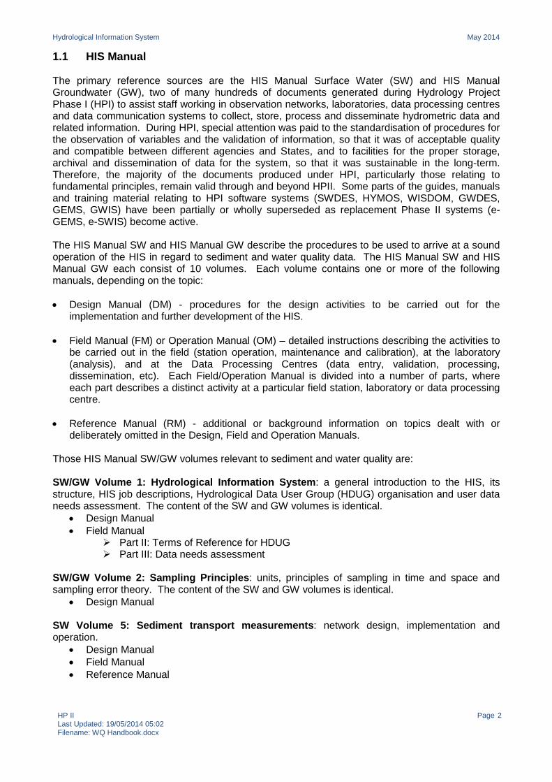
1. Introduction This Hydrology Project Phase II (HPII) Handbook provides guidance for the management of sediment and water quality data in rivers, dams/lakes/reservoirs and aquifers. The data are managed within a Hydrological Information System (HIS) that provides information on the spatial and temporal characteristics of the quantity and quality of surface water and groundwater. The information is tuned to the requirements of the policy makers, designers and researchers to provide evidence to inform decisions on long-term planning, design and management of water resources and water use systems, and for related research activities. The Indian States and Central Agencies participating in the Hydrology Project are listed in Annex I. However, this Handbook is also relevant to non-HP States. It is important to recognise that there are two separate issues involved in managing sediment and water quality information. The first issue covers the general principles of understanding monitoring networks, of collecting, validating and archiving data, and of analysing, disseminating and publishing data. The second covers how to actually do these activities using the database systems and software available. Whilst these two issues are undeniably linked, it is the first – the general principles of data management - that is the primary concern. This is because improved data management practices will serve to raise the profile of Central/State hydrometric agencies in government and in the user community, highlight the importance of sediment and water quality data for the design of water-related schemes and for water resource planning and management, and motivate staff, both those collecting the data and those in data centres. This Handbook aims to help HIS users locate and understand documents relevant to sediment and water quality in the library available through the Manuals page on the Hydrology Project website. The Handbook is a companion to the HIS manuals. The Handbook makes reference to the six stages in the hydrometric information lifecycle (Figure 1.1), in which the different processes of data sensing, manipulation and use are stages in the development and flow of information. The cycle and associated HIS protocols are explored more fully in Section 2. Subsequent sections cover different stages of the cycle for different hydro-meteorological variables.
Figure 1.1 Hydrometric information lifecycle (after: Marsh, 2002)
Hydrological Information System May 2014
HP II Last Updated: 19/05/2014 05:02 Filename: WQ Handbook.docx
Page 2
1.1 HIS Manual The primary reference sources are the HIS Manual Surface Water (SW) and HIS Manual Groundwater (GW), two of many hundreds of documents generated during Hydrology Project Phase I (HPI) to assist staff working in observation networks, laboratories, data processing centres and data communication systems to collect, store, process and disseminate hydrometric data and related information. During HPI, special attention was paid to the standardisation of procedures for the observation of variables and the validation of information, so that it was of acceptable quality and compatible between different agencies and States, and to facilities for the proper storage, archival and dissemination of data for the system, so that it was sustainable in the long-term. Therefore, the majority of the documents produced under HPI, particularly those relating to fundamental principles, remain valid through and beyond HPII. Some parts of the guides, manuals and training material relating to HPI software systems (SWDES, HYMOS, WISDOM, GWDES, GEMS, GWIS) have been partially or wholly superseded as replacement Phase II systems (e-GEMS, e-SWIS) become active. The HIS Manual SW and HIS Manual GW describe the procedures to be used to arrive at a sound operation of the HIS in regard to sediment and water quality data. The HIS Manual SW and HIS Manual GW each consist of 10 volumes. Each volume contains one or more of the following manuals, depending on the topic: • Design Manual (DM) - procedures for the design activities to be carried out for the
implementation and further development of the HIS. • Field Manual (FM) or Operation Manual (OM) – detailed instructions describing the activities to
be carried out in the field (station operation, maintenance and calibration), at the laboratory (analysis), and at the Data Processing Centres (data entry, validation, processing, dissemination, etc). Each Field/Operation Manual is divided into a number of parts, where each part describes a distinct activity at a particular field station, laboratory or data processing centre.
• Reference Manual (RM) - additional or background information on topics dealt with or
deliberately omitted in the Design, Field and Operation Manuals. Those HIS Manual SW/GW volumes relevant to sediment and water quality are: SW/GW Volume 1: Hydrological Information System: a general introduction to the HIS, its structure, HIS job descriptions, Hydrological Data User Group (HDUG) organisation and user data needs assessment. The content of the SW and GW volumes is identical.
• Design Manual • Field Manual
Part II: Terms of Reference for HDUG Part III: Data needs assessment
SW/GW Volume 2: Sampling Principles: units, principles of sampling in time and space and sampling error theory. The content of the SW and GW volumes is identical.
• Design Manual SW Volume 5: Sediment transport measurements: network design, implementation and operation.
• Design Manual • Field Manual • Reference Manual
Hydrological Information System May 2014
HP II Last Updated: 19/05/2014 05:02 Filename: WQ Handbook.docx
Page 3
SW/GW Volume 6: Water Quality sampling: network design, implementation, operation and maintenance. There are some differences in the content of the SW and GW volumes.
• Design Manual • Field Manual
SW/GW Volume 7: Water Quality analysis: laboratory procedures. The content of the SW and GW volumes is identical.
• Design Manual • Operation Manual
SW/GW Volume 8: Data processing and analysis: specification of procedures for Data Processing Centres (DPCs). The content of SW Operation Manual Part I and GW Operation Manual Part II is identical. Surface Water Volume 8: Data processing and analysis
• Operation Manual Part I: Data entry and primary validation Part II: Secondary validation Part III: Final processing and analysis Part IV: Data management
Groundwater Volume 8: Data processing and analysis
• Operation Manual Part II: Data entry and primary validation - water quality data Part V: Groundwater Year Book
SW Volume 10: Surface Water protocols: outline of protocols for data collection, entry, validation and processing, communication, inter-agency validation, data storage and dissemination, HIS training and management.
• Operation Manual Data entry forms
In this Handbook, individual parts of the HIS Manual SW/GW are referred to according to the nomenclature “SW/GWvolume-manual(part)” e.g. GW Volume 6: “Water Quality sampling” Field Manual is referred to as GW6-FM, and SW Volume 8: “Data processing and analysis” Operation Manual Part I: “Data entry and primary processing” is referred to as SW8-OM(I). A hard copy of the relevant manuals should be available for the locations listed in Annex II. For example, a hard copy of GW6-FM should be available at all groundwater monitoring stations where water quality sampling takes place. Similarly, SW8-OM(I) should be available at all Data Processing Centres where data entry and primary validation of surface water sediment and water quality data take place. As noted, there is some inevitable overlap and repetition between the HIS Manual SW and the HIS Manual GW (e.g. Volume 3). In the following sections of this Handbook, reference is generally made only to the HIS Manual SW, as the majority of sediment and water quality reference material is incorporated in here (indeed sediment is only in the HIS Manual SW), unless there is important additional information in the HIS Manual GW. 1.2 Other HPI documentation Other HPI documents of relevance to sediment and water quality include:
Hydrological Information System May 2014
HP II Last Updated: 19/05/2014 05:02 Filename: WQ Handbook.docx
Page 4
• The e-SWIS and e-GEMS software manuals, and the SWDES and GWDES software manuals - although SWDES and GWDES are being superseded by e-SWIS and e-GEMS, respectively, in HPII, to promote continuity, e-SWIS contains an eSWDES module and e-GEMS includes GWDES functionality.
• “Protocol for Water Quality Monitoring” – summary of the design approach and necessary
actions to implement water quality monitoring networks for both surface water and ground water.
• “Network and Mandates of WQ monitoring” – theme paper discussing water quality monitoring
networks for both surface water and ground water. • “Standard Analytical Procedures for Water Analyses” – summary of standard analytical
procedures for water quality analysis. • “Maintenance norms for WQ laboratories” – maintenance guidance for water quality
instrumentation and equipment. • “Surface Water Yearbook” – a template for a Surface Water Yearbook published at State level. • Water quality training modules – these are divided into five sets (see Table 1.1):
• Set I: covers surface water and groundwater sampling and on-site analysis, plus chemistry concepts and laboratory practices for Level I laboratories.
• Set II: covers pollution parameters, plus chemistry concepts and laboratory practices for Level II and II+ laboratories.
• Set III – Set V: cover chemistry concepts and laboratory practices for Level II and II+ laboratories.
• Surface water “training of trainers” modules also relevant to water quality which may be of
interest to the more advanced user (see Table 1.2).
Hydrological Information System May 2014
HP II Last Updated: 19/05/2014 05:02 Filename: WQ Handbook.docx
Page 5
Table 1.1 HPI water quality training modules Topic Module Title Set I 01 Basic water quality concepts
02 Basic chemistry concepts 03 Good laboratory practices 04 How to prepare standard solutions 05 How to measure colour odour and temperature 06 Understanding hydrogen ion concentration 07 How to measure the pH 08 Understanding EC 09 How to measure EC 10 How to measure solids 11 Chemistry of DO measurement 12 How to measure DO 13 How to sample surface waters 14 How to sample Ground Water
Set II 15 Understanding BOD test 16 Understanding dilution and seeding procedures in BOD test 17 How to measure BOD 18 Understanding COD test 19 How to measure COD 20 Introduction to Microbiology 21 Microbiological Laboratory Techniques 22 Coliforms as Indicator of Faecal Pollution 23 How to measure coliforms
Set III 24 Basic aquatic chemistry concepts 25 Oxygen balance in Surface Waters 26 Basic Ecology Concepts 27 Surface Water Quality Planning Concepts 28 Major Ions in Water 29 Advanced aquatic chemistry solubility equilibria 30 Advanced aquatic chemistry 31 Trace Compounds in the Aquatic Environment 32 Potentiometric Analysis of Water Quality 33 Use of Ion Selective Probes 34 Absorption spectroscopy 35 Emission Spectroscopy and Nephelometry 36 Measurement of Fluoride 37 Measurement of Oxidised Nitrogen 38 Measurement of Ammonia and Organic Nitrogen 39 How to measure Ammonia Nitrogen 40 Measurement of Chlorophyll-a
Set IV 41 Measurement of Phosphorus 42 Measurement of Boron 43 How to Measure Total Iron 44 How to Measure Sodium 45 How to Measure Sulphate 46 How to Measure Silicate
Set V 47 Basic Statistics 48 Applied Statistics 49 Quality Assurance and within Laboratory AQC 50 Inter-Laboratory AQC Exercise
Table 1.2 HPI water quality “training of trainers” modules Topic Module Title HIS WQ Training Specifications
Processing of Stream Flow Data
Hydrological Information System May 2014
HP II Last Updated: 19/05/2014 05:02 Filename: WQ Handbook.docx
Page 6
2. The Data Management Lifecycle in HPII Agencies and staff with responsibilities for hydrometric data have a pivotal role in the development of sediment and water quality information, through interacting with data providers, analysts and policy makers, both to maximise the utility of the datasets and to act as key feedback loops between data users and those responsible for data collection. It is important that these agencies and staff understand the key stages in the hydrometric information lifecycle (Figure 1.1), from monitoring network design and data measurement, to information dissemination and reporting. These later stages of information use also provide continuous feedback influencing the overall design and structure of the hydrometric system. While hydrometric systems may vary from country to country with respect to organisation set-ups, observation methods, data management and data dissemination policies, there are also many parallels in all stages of the cycle. 2.1 Use of sediment and water quality information in policy and decision-making The objectives of water resource development and management in India, based on the National Water Policy and Central/State strategic plans, are: to protect human life and economic functions against flooding; to maintain ecologically-sound water systems; and to support water use functions (e.g. drinking water supply, energy production, fisheries, industrial water supply, irrigation, navigation, recreation, etc). These objectives are linked to the types of data that are needed from the HIS. SW1-DM Chapter 3.3 presents a table showing HIS data requirements for different use functions on page 19. In turn, these use functions lead to policy and decision-making uses of HIS data, such as: water policy, river basin planning, water allocation, conservation, demand management, water pricing, legislation and enforcement. Hence, freshwater management and policy decisions across almost every sector of social, economic and environmental development are driven by the analysis of hydrometric information. Its wide-ranging utility, coupled with escalating analytical capabilities and information dissemination methods, have seen a rapid growth in the demand for hydrometric data and information over the first decades of the 21st century. Central/State hydrometric agencies and international data sharing initiatives are central to providing access to coherent, high quality hydrometric information to a wide and growing community of data users. Hydrological data users may include water managers or policymakers in Central/State government offices and departments, staff and students in academic and research institutes, NGOs and private sector organisations, and hydrology professionals. An essential feature of the HIS is that its output is demand-driven, that is, its output responds to the hydrological data needs of users. SW1-FM(III) presents a questionnaire for use when carrying out a data needs assessment to gather information on the profile of data users, their current and proposed use of surface water, groundwater, hydro-meteorology and water quality data, their current data availability and requirements, and their future data requirements. Data users can, through Central/State hydrometric agencies, play a key role in improving hydrometric data, providing feedback highlighting important issues in relation to records, helping establish network requirements and adding to a centralised knowledge base regarding national data. By embracing this feedback from the end-user community, the overall information delivery of a system can be improved. A key activity within HPII was a move towards greater use of the HIS data assembled under HPI. Two examples of the use of HIS data include the Purpose-Driven Studies (PDS) and the Decision Support Systems (DSS) components of HPII. See the Hydrology Project website for more information about DSS and PDS, and access to PDS reports. The 38 PDS, which were designed, prepared and implemented by each of the Central/State
Hydrological Information System May 2014
HP II Last Updated: 19/05/2014 05:02 Filename: WQ Handbook.docx
Page 7
hydrometric agencies, are small applied research projects to investigate and address a wide range of real-world problems and cover surface water, groundwater, hydro-meteorology and water quality topics. Some examples of projects include a study of reservoir sedimentation and development of a catchment area treatment plan for the Kodar Reservoir in Chhattisgarh (PDS number SW-CH-1), and a study of groundwater quality in the Jabalpur urban area in Madhya Pradesh, with an emphasis on transport of pathogenic pollutants (PDS number SW-NIH-1). The PDS utilise hydrometric data and products developed under HPI, supplemented with new data collected during HPII. Two separate DSS programmes were set up under HPII. One, for all participating implementing agencies, called DSS Planning (DSS-P), has established water resource allocation models for each State to assist them to manage their surface and groundwater resources more effectively. The other, called DSS Real-Time (DSS-RT) was specifically for the Bhakra-Beas Management Board (BBMB), although a similar DSS-RT study has also now been initiated on the Bhima River in Maharashtra. The DSS programmes have been able to utilise hydrological data assembled under the Hydrology Project to guide operational decisions for water resource management. 2.2 Sediment and water quality monitoring network design and development Section 3.2 of this Handbook outlines the design and development of sediment and water quality monitoring networks. Networks are planned, established, upgraded and evolved to meet a range of needs of data users and objectives, most commonly water resources assessment and hydrological hazard mitigation (e.g. flood forecasting). It is important to ensure that the hydro-meteorological, surface water, groundwater and water quality monitoring networks of different agencies are integrated as far as possible to avoid unnecessary duplication. Integration of networks implies that networks are complimentary and that regular exchange of data takes place to produce high quality validated datasets. Responsibility for maintenance of Central/State hydrometric networks is frequently devolved to a regional (Divisional) or sub-regional (Sub-Divisional) level. 2.3 Data sensing and recording Sections 3.1-3.4 of this Handbook review sediment and water quality monitoring networks and stations, maintenance requirements and measurement techniques. Responsibility for operation of Central/State hydro-meteorological monitoring stations is frequently devolved to a regional (Divisional) or sub-regional (Sub-Divisional) level. However, it is important that regular liaison is maintained between sub-regions and the Central/State agencies through a combination of field site visits, written guidance, collaborative projects and reporting, in order to ensure consistency in data collection and initial data processing methods across different sub-regions, maintain strong working relationships, provide feedback and influence day-to-day working practice. Hence, the Central/State agencies are constantly required to maintain a balance of knowledge between a broad-scale overview and regional/sub-region sediment and water quality awareness. Operational procedures should be developed in line with appropriate national and international (e.g. Indian, ISO, WMO) standards (e.g. WMO Report 168 “Guide to Hydrological Practices”). 2.4 Data validation and archival storage The quality control and long-term archiving of sediment and water quality data represent a central function of Central/State hydrometric agencies. This should take a user-focused approach to improving the information content of datasets, placing strong emphasis on maximising the final utility of data e.g. through efforts to improve completeness and fitness-for-purpose of Centrally/State archived data. Section 3.5 of this Handbook summarises the stages in the
Hydrological Information System May 2014
HP II Last Updated: 19/05/2014 05:02 Filename: WQ Handbook.docx
Page 8
processing of sediment and water quality data. Sections 4 and 5 of this Handbook cover the process from data entry through primary and secondary validation, and also compilation and analysis of data (Section 2.5), for sediment and water quality data, respectively. During all levels of validation, staff should be able to consult station metadata records detailing the history of the site and its performance, along with topographical, hydrogeological and isohyetal maps and previous quality control logs. Numerical and visual tools available at different phases of the data validation process, such as versatile time series plotting and manipulation software, and assessment of time series statistics greatly facilitate validation. High-level appraisal by Central/State staff, examining the data in a broader spatial context, can provide significant benefits to final information products. It also enables evaluation of the performance of sub-regional data providers, laboratories, individual stations or groups of stations, which can focus attention on underperforming sub-regions and encourage improvements in data quality. A standardised data assessment and improvement procedure safeguards against reduced quality, unvalidated and/or unapproved data reaching the final data archive from where they can be disseminated. However, Marsh (2002) warns of the danger of data quality appraisal systems that operate too mechanistically, concentrating on the separate indices of data quality rather than the overall information delivery function. For the Hydrology Project, the timetable for data processing is set out in SW10-OM Protocols and Procedures for sediment and surface water quality samples and data, and in GW10-OM HIS activities – Groundwater domain for groundwater quality samples and data, and summarised in Table 2.1 of this Handbook. Sample analysis is required to be completed at the laboratory within the allowed time period for the specified water quality parameters, and data entry to be completed immediately the analysis results are available. Primary validation, also by the laboratory, should be completed within one week of data entry. Initial secondary validation, in State DPCs for State data, and CWC/CGWB/CPCB local offices for Central data, should be completed within one month of data entry. Some secondary validation will not be possible until the end of the hydrological year when the entire year’s data can be reviewed in a long-term context, and compared with Central data, so data should be regarded as provisional approved data until then, after which data should be formally approved and made available for dissemination to external users. At certain times of year (e.g. during the monsoon season), this data processing plan may need to be compressed, so that validated sediment and water quality data are available sooner. Table 2.1 Sediment and water quality data processing timetable for data for month n Activity Responsibility Deadline Sediment and water quality data Sample receipt and analysis Laboratory Within allowed time period Data entry Laboratory Same day as analysis Primary validation Laboratory Within 1 week of data entry Secondary validation State DPC
State DPC
Initial - Within 1 month of data entry Final – end of hydrological year + 3 months
Compilation State DPC As required Analysis State DPC As required Reporting State DPC At least annually Data requests State DPC 95% - within 5 working days
5% - within 20 working days Interagency validation IMD At least 20% of State stations, on
rolling programme, by end of hydrological year + 6 months
Hydrological Information System May 2014
HP II Last Updated: 19/05/2014 05:02 Filename: WQ Handbook.docx
Page 9
2.5 Data synthesis and analysis Central/State hydrometric agencies play a key role in the delivery of large-scale assessments of sediment and water quality data. Through their long-term situation monitoring, they are often well placed to conduct or inform scientific analysis at a State, National or International level, and act as a source of advice on data use and guidance on interpretation of data. This is especially true in the active monitoring of the State or National situation or the assessment of conditions at times of extreme events (e.g. monsoonal rains, droughts) which may have a significant impact on water quality, where agencies may be asked to provide input to scientific reports and research projects, as well as informing policy decisions, media briefings, and increasing public understanding of the state of the water environment. Sections 4 and 5 of this Handbook cover compilation and analysis of data, as well as the process from data entry through primary and secondary validation (Section 2.4), for sediment and water quality data, respectively. 2.6 Data dissemination and publication One of the primary functions of Central/State hydrometric agencies is to provide comprehensive access to information at a scale and resolution appropriate for a wide range of end-users. However, improved access to data should be balanced with a promotion of responsible data use by also maintaining end-user access to important contextual information. Thus, the dissemination of user guidance information, such as composite summaries that draw users’ attention to key information and record caveats (e.g. monitoring limitations, levels of uncertainty regarding data accuracy, major changes in laboratory setup), is a key stewardship role for Central/State hydrometric agencies, as described in Section 6 of this Handbook. For large parts of the 20th century the primary data dissemination route for sediment and water quality data was via annual hardcopy publications of data tables i.e. yearbooks. However, the last decade or so has seen a shift towards more dynamic web-based data dissemination to meet the requirement for shorter lag-time between observation and data publication and ease of data re-use. Like many countries, India now uses an online web-portal as a key dissemination route for hydrometric data and associated metadata which provides users with dynamic access to a wide range of information to allow selection of stations. At least 95% of data requests from users should be processed within 5 working days. More complex data requests should be processed within 20 working days. 2.7 Real-time data During HPII many implementing agencies developed low cost real-time data acquisition systems, feeding into bespoke databases and available on agency websites. Such systems often utilise short time interval recording of data e.g. 15 minutes, 1 hour, etc. In some instances, agencies are taking advantage of the telemetry aspect of real-time systems as a cost-effective way of acquiring data from remote locations. However, for some operational purposes (e.g. real-time flood forecasting, water abstraction, etc), real-time data may need to be used immediately. Real-time water quality data should go through some automated, relatively simple data validation process before being input to real-time models e.g. checking that each incoming data value is within pre-set limits for the station, and that the change from preceding values is not too large. Where data fall outside of these limits, they should generally still be stored, but flagged as suspect, and a warning message displayed to the model operators. Where suspect data have been identified, a number of options are available to any real-time forecasting or decision support model being run, and the choice will depend upon the modelling requirements. Whilst suspect data could be accepted and the model run as normal, it is more common to treat suspect data as missing or to substitute them with some form of back-up, interpolated or extrapolated data. This is necessary for
Hydrological Information System May 2014
HP II Last Updated: 19/05/2014 05:02 Filename: WQ Handbook.docx
Page 10
hydrometric agencies to undertake some of their day-to-day functions and, in such circumstances, all the data should be thoroughly validated as soon as possible, according to the same processing timetable and protocols as other climate data. Real-time water quality data should also be regularly transferred to the e-SWIS or e-GEMS database system, through appropriate interfaces, in order to ensure that all data are stored in a single location and provide additional back-up for the real-time data, but also to provide access to the data validation tools available through the software systems.
Hydrological Information System May 2014
HP II Last Updated: 19/05/2014 05:02 Filename: WQ Handbook.docx
Page 11
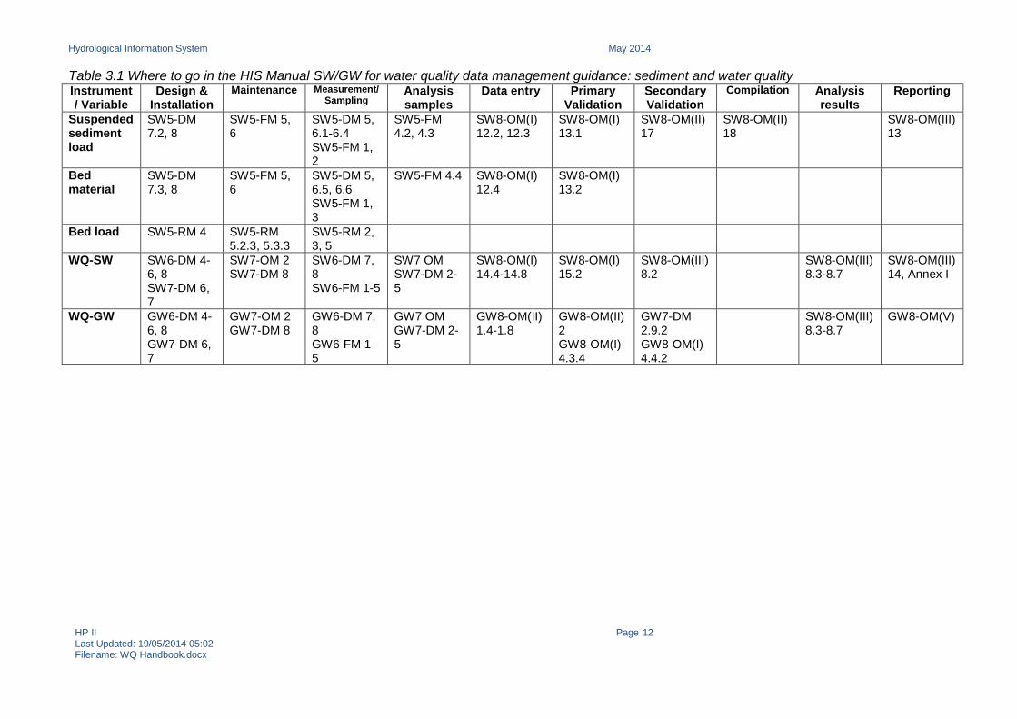
3. Sediment and Water Quality Monitoring Stations and Data 3.1 Monitoring stations For sediment and water quality monitoring stations, Table 3.1 lists the relevant section in the HIS Manual SW and HIS Manual GW for detailed information on design and installation, maintenance, measurement/sampling, analysis of samples, data entry, validation, compilation and analysis of results, and reporting. A set of specifications for hydrometric equipment was compiled under HPI and updated under HPII. The specifications, which are downloadable from the Hydrology Project website, provide a guideline for procurement, some technical guidance for which is offered in SM4-DM Chapter 7 (with examples of some procurement templates and documents also on the Hydrology Project website). 3.1.1 Sediment monitoring stations Knowledge of sediment transport in a river is essential for the solution of variety of problems associated with flow in rivers: • Estimation of sediment inflow into reservoirs at the planning and design stage - by estimating
the suspended load and bed loads separately • Studies for river training and river regimes – data may have to be gathered by mounting
intensive observation campaigns for short periods • Evaluation of basin erosion and identification of conservation measures • Estimation of regime widths and scour depths for barrages bridges from bed material analysis Hence, sediment data helps verify existing theories and empirical formulae for computation of sediment transport, and leads to better problem solving and design of water use facilities. Types of sediment include: • Suspended sediment load – sediment maintained in suspension by turbulence in flowing water
for considerable periods of time without contact with the channel bed. It moves with practically the same velocity as that of the flowing water. Suspended sediment is routinely split into three class sizes: coarse > 2 mm; medium 0.075-2 mm; and fine <0.075 mm.
• Bed material – material, the participles of which are found in appreciable quantities in that part
of the channel bed affected by transport. • Bed load – sediment in almost continuous contact with the channel bed, carried forward by
rolling, sliding and/or hopping. Sediment measurements are relatively difficult to make. The direct measurement method, used in India, aims at determining the weight or volume of sediment passing a section in a period of time. The alternative indirect measurement method aims at measuring the concentration of sediment flowing in the moving water, and needs the measurement of sediment concentrations, the cross-sectional areas and flow velocities, as well as the sediment being transported as wash load and bed load. Routine sediment measurements are usually restricted to sampling the suspended load at flow gauging stations. In this sense, sediment is looked at as a “quality” parameter of the water.
Hydrological Information System May 2014
HP II Last Updated: 19/05/2014 05:02 Filename: WQ Handbook.docx
Page 12
Table 3.1 Where to go in the HIS Manual SW/GW for water quality data management guidance: sediment and water quality Instrument/ Variable
Design & Installation
Maintenance Measurement/Sampling
Analysis samples
Data entry Primary Validation
Secondary Validation
Compilation Analysis results
Reporting
Suspended sediment load
SW5-DM 7.2, 8
SW5-FM 5, 6
SW5-DM 5, 6.1-6.4 SW5-FM 1, 2
SW5-FM 4.2, 4.3
SW8-OM(I) 12.2, 12.3
SW8-OM(I) 13.1
SW8-OM(II) 17
SW8-OM(II) 18
SW8-OM(III) 13
Bed material
SW5-DM 7.3, 8
SW5-FM 5, 6
SW5-DM 5, 6.5, 6.6 SW5-FM 1, 3
SW5-FM 4.4 SW8-OM(I) 12.4
SW8-OM(I) 13.2
Bed load SW5-RM 4 SW5-RM 5.2.3, 5.3.3
SW5-RM 2, 3, 5
WQ-SW SW6-DM 4-6, 8 SW7-DM 6, 7
SW7-OM 2 SW7-DM 8
SW6-DM 7, 8 SW6-FM 1-5
SW7 OM SW7-DM 2-5
SW8-OM(I) 14.4-14.8
SW8-OM(I) 15.2
SW8-OM(III) 8.2
SW8-OM(III) 8.3-8.7
SW8-OM(III) 14, Annex I
WQ-GW GW6-DM 4-6, 8 GW7-DM 6, 7
GW7-OM 2 GW7-DM 8
GW6-DM 7, 8 GW6-FM 1-5
GW7 OM GW7-DM 2-5
GW8-OM(II) 1.4-1.8
GW8-OM(II) 2 GW8-OM(I) 4.3.4
GW7-DM 2.9.2 GW8-OM(I) 4.4.2
SW8-OM(III) 8.3-8.7
GW8-OM(V)
Hydrological Information System May 2014
HP II Last Updated: 19/05/2014 05:02 Filename: WQ Handbook.docx
Page 13
3.1.2 Water quality monitoring stations Water quality is an indicator of the physical, chemical and/or biological state of water, determined by insitu measurement in the field and/or laboratory analysis for one or more parameters of interest. Water quality may be related to the suitability of water for a particular use or purpose, and the most critical step in a successful water quality monitoring programme is a clear definition and specification of the monitoring objectives and information needs for water management: • Building up an overall picture of the aquatic environment thus enabling pollution cause and
effect to be judged • Providing long-term background data against which future changes can be assessed • Detecting trends • Providing warnings of potentially deleterious changes • Checking for compliance or for charging purposes • Precisely characterising an effluent or water body (possibly to enable classification to be
carried out) • Investigating pollution • Collecting sufficient data to perform in-depth analysis (e.g. mathematical modelling) or to allow
research to be carried out The design of the water quality monitoring programme involves the selection of water sampling locations, sampling frequency and water quality parameters to generate the required information. Sampling locations may be many and varied as water quality may be compromised through direct point sources, diffuse agricultural sources and diffuse urban sources: • Rivers – issues may include changes in physical characteristics (i.e. temperature, turbidity,
total suspended solids) and river hydrology, contamination by faecal and organic matter, contamination by toxic pollutants (i.e. organics and heavy metals), river eutrophication, salinisation, contamination by agrochemicals, and mining activities.
• Dams/lakes/reservoirs – issues may include pollution from riverine, groundwater and/or
atmospheric sources, eutrophication, acidification, and bioaccumulation and biomagnification. • Aquifers – issues may include contamination by faecal and organic matter, contamination by
toxic pollutants (i.e. organics and heavy metals), overabstraction, contamination by agrochemicals, and mining activities.
A total of 68 water quality parameters are analysed as standard parameters under the Hydrology Project. These fall into several groups: • General - basic parameters many of which can be measured instrumentally either in the field or
in the laboratory e.g. temperature, conductivity, pH, DO • Nutrients - nitrogen and phosphorus parameters which will measure the nutrients available for
plant growth and eutrophication • Organic matter - parameters capable of estimating the likely effect on watercourses of the
discharge of organic matter i.e. BOD and COD • Major ions - the inorganic anions and cations which can describe the chemical composition of
the water and help to assess pollution • Other inorganics - miscellaneous inorganic species which are important for certain water uses
or for classification purposes • Metals - metal species which are important because of their toxicity or because they are useful
indicators of the presence of other metals i.e. cadmium, zinc and mercury • Organics - particular species which are important due to their toxicity, effect on potability of
water or effect on the natural river processes e.g. pesticides
Hydrological Information System May 2014
HP II Last Updated: 19/05/2014 05:02 Filename: WQ Handbook.docx
Page 14
• Microbiological – total coliforms as an indicator species for the presence of faecal pollution of water
• Biological – chlorophyll a, present in plants, as an indicator of algal growth and, therefore, eutrophication of waters
Some potentially important parameters are not in this list: e.g. heavy metals such as lead, copper, nickel, arsenic, chromium; organic pollutants such as polychlorinated biphenyls (PCBs) and certain types of pesticide; certain organic solvents; and oils and hydrocarbons. For each basin it may be necessary to ascertain whether or not any of these pollutants are present in unacceptable concentrations and should be added to the parameter list for that sampling location. 3.2 Monitoring networks and laboratories Monitoring networks should be considered to be dynamic entities. It is important that the current utility of well-established monitoring networks is periodically assessed to ensure that they continue to meet changing requirements and to optimise the information they deliver. Network reviews should be done in collaboration with other agencies, including CPCB, CWC and CGWB. SW5-DM Chapters 3 and 4 describe network design and optimisation for sediment monitoring, and SW/GW6-DM Chapters 4 to 6 for water quality. Sediment and water quality monitoring sites are often at flow gauging stations. Whilst priority may be given to the requirements of the surface water network (Water Level, Stage-Discharge and Flow Handbook, Section 3.2) or groundwater network (Groundwater Handbook, Section 3.2), there are several advantages: flow or groundwater level data are available which provides important information for data analysis; generally, the site will be easily accessible and well-maintained; and any changes at or near the site will be noted. For more detailed information see: SW/GW2-DM Chapter 7 which provides some generic guidance on types of network and the steps in network design; SW/GW2-DM Chapters 3.2.1 to 3.2.6 which describe classification of stations and offer some examples of types of network; and Surface Water Training Module 45 “How to review monitoring networks”. A good example of a monitoring network review under HPII is the Purpose Driven Study (PDS) on optimisation of the river gauging station and raingauge networks in Maharashtra (PDS number SW-MH-1). 3.2.1 Sediment monitoring networks A sediment monitoring network is a system of flow and sediment gauging stations in a river basin that provides data needed for the planning, design and management of the water resources in the basin from the point of view of the sediment. There are no specific requirements in terms of minimum basin area, but all the sediment sources of importance for establishing sediment balances should be included in the network. All primary flow stations should have sediment measured together with the flow, if feasible, but not necessarily at the same location as the flow gauging station. They should all comprise at least suspended load measurement. However, sediment monitoring stations are expensive to equip and to operate, so network optimisation should rather be based on sound judgement and economic consideration (cost-effectiveness). Possible questions to be addressed when selecting sediment measuring sites include: • What is the purpose of the station: e.g. monitoring of reservoir sedimentation, planning and
design of structures, setting up sediment balances in river reaches? • What are the sediment conditions at the site: i.e. how variable are sediment transport rates in
the river reach, are there preferential zones of scour and/or deposition? • In what range of flow should the sediment be gauged, and which part of the load: e.g. no bed
load during the lean season? • What size fractions are needed: e.g. the wash load not of interest for a problem of river
morphology?
Hydrological Information System May 2014
HP II Last Updated: 19/05/2014 05:02 Filename: WQ Handbook.docx
Page 15
• What level of accuracy should be attempted, for the various transport modes and for the various size fractions?
• What period of record is required and what frequency of measurement is desirable, possibly in particular phases of the hydrograph: e.g. more frequent sampling during the rising limb of the hydrograph?
• Who are the possible users and for which kind of data? • Are there limitations in terms of access to the site and transport of the samples to the
laboratory for analysis? • What are the constraints in terms of resources (human and financial)? • What are the possible preferences for equipment and methodology: e.g. existing experience
with one or another type of instrument; proximity of a research centre that can assist in case of difficulties for implementing the measurements?
SW5-DM devotes Chapter 4.2 to the topic of site surveys for sediment measuring sites, which comprise three phases: a desk study, a reconnaissance survey and other surveys e.g. trial sampling. The site survey, which should be carried out in collaboration with CWC, may reveal that the desired location is unsuitable, and an alternative site may need to be considered. SW5-DM Chapter 4.2.6 presents a useful list of criteria that should be taken into consideration in selecting a site to ensure long-term reliable data. Because the majority of sediment measuring sites will be at flow gauging stations, the station design, construction and installation procedures for flow gauging stations should be followed (Water Level, Stage-Discharge and Flow Handbook, Section 3.2). 3.2.2 Water quality monitoring networks A water quality monitoring network is a system of water quality monitoring sites in a river basin, aligned with the flow monitoring network and/or located at boreholes, that provides information on the actual status and trends that are relevant for the functions and uses of the river, reservoir or aquifer. Water quality monitoring networks are classified as: • Monitoring i.e. long-term standardised measurement in order to define status and trends – with
sub-categories: baseline, trend and flux. See SW6-DM Chapter 4.2.2 or GW6-DM Chapter 4.2.1 for more information.
• Surveillance i.e. continuous specific measurement for the purpose of water quality management and operational activities – with sub-categories: water use and pollution control. See SW6-DM Chapter 4.2.3 or GW6-DM Chapter 4.2.1 for more information.
• Survey i.e. a finite duration intensive programme to measure for a specific purpose – with subcategories: classification, and management and research. See SW6-DM Chapter 4.2.4 or GW6-DM Chapter 4.2.1 for more information.
New water quality monitoring stations should be a combination of baseline and trend stations with samples collected every two or three months. After data have been collected for three years, the stations should be reclassified either as baseline, trend or flux station. A baseline station should be monitored at least every two or three months, a trend station at least once every month, and a flux station more regularly e.g. 12 or 24 times per year. The monitoring network is defined by the density of stations (how many locations on a certain river-stretch or in a certain aquifer are investigated, and what are the locations?), the frequency of sampling (how many samples per year are collected from each location?), and the list of water quality parameters that are analysed for each sample collected. The density, sampling frequency and parameters for each of the water quality monitoring network classes and sub-categories are listed in Table 4.1 on page 17 of SW/GW6-DM and the subsequent Tables 4.2-4.4 of the SW volume.
Hydrological Information System May 2014
HP II Last Updated: 19/05/2014 05:02 Filename: WQ Handbook.docx
Page 16
Surface water quality monitoring network design and evaluation is a multi-step process, comprising: 1. Construction of a base map with river basin boundaries, state boundaries, national boundaries,
and rivers, dams and lakes 2. Classification of the main stem and major tributaries (contributing more than 20% of the flow of
the main stem at the confluence point) 3. Construction of overlays with geological information e.g. rock types, and with pollution sources
e.g. major towns, industrial centres, agricultural land 4. Positioning of baseline (monitoring) stations - each major tributary should have a baseline
station to get a good overall picture of the (natural) background concentration of various constituents of water in rivers in the basin. Baseline stations should be positioned in relatively unpolluted areas such as upstream of major towns and industrial centres.
5. Positioning of trend (monitoring) stations – trend stations are located on the main stem when the river flow increases by 20% of the flow at the previous station. In the case of confluence with a major tributary, trend stations are located both on the tributary and on the main stem of the river, just above the confluence point.
6. Positioning of flux stations to gauge the load of anthropogenic pollutants passing a sampling point.
7. Critical review of the monitoring network so far e.g. check that the distance between successive trend stations on the main stem is not too short
8. Review of existing networks of CWC, CGWB and State agencies – construct an overlay with the locations of water quality monitoring stations of CWC, CGWB and State agencies e.g. irrigation department
9. Review of existing network of CPCB - construct an overlay with the locations of water quality monitoring stations of CPCB
10. Rationalisation of networks – where comparison of monitoring networks reveals a duplication of effort, dialogue between organisations should be initiated to review the networks compared to: the information needs of hydrological data users; the station location, sampling frequency and parameters; the availability of the current and historical data in the public domain; a comparison of historical data; the validity of the data; and a comparison of the analytical quality control programmes employed by the laboratories.
11. Adding Surveillance and Survey type stations – if required by the mandate 12. Identifying sampling frequency and water quality parameters for analysis, keeping in mind the
objectives, feasibility of sampling, costs and above all capacity of field staff and laboratories. Groundwater quality monitoring network design and evaluation has some similarities with the surface water network. Groundwater quality monitoring networks usually correspond with groundwater level monitoring networks of observation wells. For water quality monitoring stations, it is essential that the water is pumped, so that the water in the well represents the aquifer water and not storage water. A groundwater quality monitoring network should take into account features of the area or region that are likely to have an impact on the water quality e.g. for a groundwater quality network, these might include aquifer geology, type of aquifer, land use patter, geological set up, geomorphological set up, and drainage basin. A simple approach to locating monitoring stations is to mark the boundaries of the relevant features on a map and locate at least one station in each intersection. For example, if an area has two aquifer geological formations, shale and limestone, and two types of land use, agricultural and fallow, their intersection would yield up to four unique possibilities (shale-agriculture, shale-fallow, limestone-agriculture, limestone-fallow) and the network should have at least one station in each of the intersections. Network rationalisation (step 10 under surface water above) is common to any monitoring network as periodic analysis and review of data is may lead to new or redefined information needs, which may be translated into different sampling locations, sampling frequency and/or parameters. Rationalisation within a single organisation, or between networks of multiple organisations, may free up resources which may be directed towards an increase in frequency of measurement for
Hydrological Information System May 2014
HP II Last Updated: 19/05/2014 05:02 Filename: WQ Handbook.docx
Page 17
greater reliability and/or introduction of new water quality parameters for characterisation. To inform rationalisation, the following types of data analyses should be made: • Is there a correlation between different parameters at one station? If there is a good
correlation between two or more parameters, then possibly one or more parameters could be dropped from the parameter list, saving analysis effort. The values for the dropped parameter(s) should then be estimated from the remaining, measured parameter. Examples of possible parameter correlation are BOD-COD, EC-major cations/anions, etc.
• Is there a correlation between water quality parameter(s) and river flow at a station (surface water stations)? If there is a good correlation, then water quality information could be approximated at all times that flow data are available. This can supply additional water quality information at times between sampling events, without additional sampling effort.
• Is there a correlation in parameters between 2 (or more) stations? If such a correlation exists, then one of the stations could be dropped, thus saving on sampling and analysis effort. The water quality information for the dropped station should then be estimated from the parameters at the measured station. Alternatively, the redundant sampling station could be moved to a new location where unique water quality information will be gained.
• Is the sampling frequency sufficient to meet the monitoring objectives (e.g. if an objective is trend detection, is the frequency high enough to be able to detect trends?). Analysis of the data with respect to the monitoring objectives may result in a raising or lowering of sampling frequency.
• Does monitoring of surveillance or survey category monitoring indicate any new water quality issues which should be taken up in monitoring category (i.e. flux or trend type)? If so, new locations and/or parameters may be added for monitoring, that is to say, the network design can be adapted.
Rationalisation of a network may usually be done only after 3 to 5 years of data collection when sufficient historical data are available for analysis. SW6-DM Chapter 4.3 describes design of a water quality monitoring network in the Mahanadi basin in Madhya Pradesh, Orissa, Bihar and Maharashtra. SW6-DM Chapter 5.5 describes rationalisation of a surface water quality monitoring network in the Cauvery basin in Karnataka and Tamil Nadu, and GW6-DM Chapter 5.5 describes rationalisation of a groundwater quality monitoring network in the Ghataprabha basin in Karnataka. Because the majority of water quality monitoring sites will be at existing flow gauging stations or observation wells, the station design, construction and installation procedures for flow gauging stations or observations wells should be followed (Water Level, Stage-Discharge and Flow Handbook, Section 3.2 or Groundwater Handbook, Section 3.2, respectively). In addition, SW6-DM devotes Chapter 6 to the topic of selecting sampling sites for surface water quality monitoring. The site survey, which should be carried out in collaboration with CWC and/or CPCB, may reveal that the desired location is unsuitable, and an alternative site may need to be considered. SW5-DM Chapter 6.1 presents a useful list of criteria that should be taken into consideration in selecting a site to ensure long-term reliable data. 3.2.3 Laboratories Water quality laboratories of different levels were established under the Hydrology Project. The level of the laboratory is an indication of the analytical capacity of the laboratory based on the equipment available, and not necessarily linked to the actual number of parameters analysed i.e. it represents the potential capability of the laboratory: • Level I – small laboratory located at or near the monitoring site (field), generally analysing
temperature, pH, conductivity, total suspended solids, Dissolved Oxygen (DO), colour and odour (these parameters may also be measured in the field at the time of sampling)
• Level II - laboratory servicing larger area, with facilities to analyse general water quality parameters, major ions, nutrients, indicators of organic and faecal pollution, etc.
Hydrological Information System May 2014
HP II Last Updated: 19/05/2014 05:02 Filename: WQ Handbook.docx
Page 18
• Level II+ - laboratory servicing larger area, in possession of advanced equipment such as Atomic Adsorption Spectrophotometer (AAS), Gas Chromatograph (GC), or UV-Visible Spectrophotometer etc.
Laboratories should keep records of any malfunctioning and breakdown of equipment (with dates), dates of equipment maintenance, power failure events and their duration, within-laboratory analytical quality control (AQC; see Section 3.3.2) results and control chart results for different parameters, and results of participation in inter-laboratory AQC. 3.3 Inspections, audits and maintenance Regular maintenance of sampling and analysis equipment, together with periodic inspections and audits, ensures collection of good quality sediment and water quality data and provides information that may assist in future data validation queries. Table 3.1 lists the relevant section in the HIS Manual SW and HIS Manual GW for maintenance of the different types of sediment and water quality stations and instruments. For sediment, this topic is largely covered in different chapters of SW5-FM for field inspections and audits, and for routine maintenance and calibration of equipment. For water quality, this topic is covered in the document “Maintenance norms for WQ laboratories” which is a maintenance guide for surface water and groundwater quality instrumentation and equipment. 3.3.1 Sampling equipment Maintenance and calibration requirements for instruments and equipment are often item-specific. For example, if suspended sediment is sampled with a bottle sampler, calibration of the equipment itself is not required, but an inter-comparison of the data obtained with the instrument with results of other sampling equipment is required for interpretation purposes. A supply of appropriate spare sampling equipment and parts should be kept on site and/or taken on field visits in case they are needed. SW/GW6-FM Table 2.1 provides a checklist for a field visit. For sediment monitoring at flow gauging stations, SW5-FM Chapter 6.3 lists maintenance norms, including maintenance of civil works, maintenance of equipment, costs of consumable items and payments to staff (where the costs should be regarded as out of date), in addition to the maintenance norms for the flow monitoring stations themselves (Water Level, Stage-Discharge and Flow Handbook, Section 3.3). 3.3.2 Laboratories The importance of the quality assurance (QA) is recognised in any water quality monitoring programme, and is an essential part of analytical work. A laboratory contains a variety of equipment ranging from simple heating devices to extremely sophisticated computer-controlled analytical equipment. It is a good practice to keep a separate logbook for each major piece of equipment where details of its use, maintenance schedule, breakdowns and repairs, accessories, supply of consumables, etc., are carefully entered. Such a record will help in properly maintaining the instrument and planning for future. Each analyst in each laboratory should follow established procedures to detect and to correct problems and take every reasonable step needed to keep the measurement process reliable. The more important features of a QA programme should include: • Use of documented methods of analyses • Properly maintained and calibrated equipment • Properly trained staff • Effective internal quality control (within-laboratory analytical quality control (AQC)) • Participation in periodic programmes for evaluation of measurement bias (inter-laboratory
AQC)
Hydrological Information System May 2014
HP II Last Updated: 19/05/2014 05:02 Filename: WQ Handbook.docx
Page 19
• External assessment by accreditation or other compliance schemes SW/GW7-OM Table 2.3 presents examples of specific sources of error for the analyses of TDS, TH, EC, fluoride, sulphate, phosphate, nitrate, sodium and boron. 3.4 Data sensing and recording Table 3.1 lists the relevant section in the HIS Manual SW and HIS Manual GW for operational instructions on the sampling and subsequent analysis for sediment and water quality. 3.4.1 Sediment sampling and analysis Selecting appropriate sediment sampling frequency is critical, because the main part of the sediment fluxes occurs during flood events, when sediment measurements are most difficult to make. For the lower reaches of flash flood rivers, the fluxes during flood events may be close to 100% of the total yearly sediment discharge. Suspended sediment is likely to be observed even during the non-monsoon season in the form of wash load, but bed material movement will be initiated above a certain threshold level and should often be nil or negligible during the non-monsoon season. Suspended sediment data comprise of the concentrations of coarse (> 0.2 mm), medium (0.075-0.2 mm) and fine (< 0.075 mm) material in combination with water level and flow data. The suspended sediment concentration of the flow is determined by collecting depth integrated samples that define the mean flow-weighted concentration in the sample vertical, from a sufficient number of verticals to define the mean flow-weighted concentration in the cross-section. The suspended sediment concentrations are usually obtained from point samples by the Punjab bottle sampler (other bottle-type point samplers and alternative fixed volume depth-integrating samplers and point-integrating samplers are also available) taken at 0.6 of the water depth in a number of verticals in the cross-section, and normally collected during flow gauging (alternative approaches take several sediment samples in each vertical, at 0.2d, 0.5d, 0.6d and 0.8d where samples are subsequently combined). SW5-FM Chapter 2 discusses the various different sampling instruments for suspended sediment and bed material, including instructions for use and precautions before, during and after sampling, and advantages and limitations. The two methods for determining the concentration in the cross-section are the equal discharge increment (EDI) method where the cross-section is divided into unequally spaced segments of equal discharge describing the cross-sectional variation in concentration, and the equal width increment (EWI) method where the cross-section is divided into equally spaced segments. Recommendations for the minimum number of verticals given by the Bureau of Indian Standards are at least 3 vertical for rivers < 30 m in width, at least 5 vertical for rivers between 30 m and 300 m wide, and at least 7 verticals for rivers > 300 m in width. Sampling may take place by wading, from a bridge, from a boat, or from a cableway. Per fraction, a flow-weighted average concentration is computed in the field laboratory and entered in the field data sheet. If samples are collected with only water level measurement, the corresponding flows are computed later using the station rating curve. Suspended sediment samples are analysed in the water quality laboratory by a gravimetric procedure. Bed material samples are generally collected thrice in a water year: pre-monsoon, monsoon and post-monsoon. Surface samples are collected using scoop-type, grab-type and dredge-type devices and pumps. SW5-FM Chapter 2 discusses the various different sampling instruments for suspended sediment and bed material, including instructions for use and precautions before, during and after sampling, and advantages and limitations. Sub-surface samples are collected using (piston) corers or from a pit in a dry bed. Bed-material samples are often collected in conjunction with flow gauging and/or a set of suspended sediment samples. By taking these
Hydrological Information System May 2014
HP II Last Updated: 19/05/2014 05:02 Filename: WQ Handbook.docx
Page 20
samples at the same stationing points, any change in bed material or radical change in flow across the stream that would affect the sediment discharge computations can be accounted for by subdividing the stream cross-section at one or between two of the common verticals. As samples are obtained across the channel, they should be visually checked and compared with the previous samples to see if the material varies considerably in size from one location to the next. Bed material samples should be labelled properly for future identification, and to provide important information useful in the laboratory analysis and the preparation of records. Bed material samples are analysed in the water quality laboratory in two ways: for particle sizes > 0.6 mm by dry sieving, and for particle sizes < 0.6 mm by siltometer. Bed load samples are difficult to obtain, requiring extensive training in proper operation and maintenance of bed load instruments and gauging strategies to get the most representative samples and measurements, and are not covered further in this Handbook. See SW5-RM for more information. Observations of sediment should be daily for at least one or two years, until the stability of the site (i.e. the relationship between suspended sediment concentration and flow, and an understanding of the size and nature of the bed material and bed load) is established, after which sampling frequency may be reduced during the non-monsoon season. However, in cases such as flash flood rivers, irregular sediment input downstream from mines, landslide-prone areas , artificial drainage systems, etc, sampling may be more times a day, up to hourly. 3.4.2 Water quality sampling and analysis SW6-FM Figure 3.4 provides a sample identification form for surface water samples which records all important information concerning the sample collected, including local conditions at the time of sampling. GW6-FM Table 4.1 provides an equivalent sample identification form for groundwater samples. The sample identification form should be given to the laboratory with the water sample. Sampling location, sampling frequency and the required water quality parameters depends upon the class and sub-category of the water quality monitoring network (Section 3.2.2). For surface water in rivers and dams/lakes/reservoirs, grab samples are collected in allocated containers from approximately 20 cm below the water surface, taking care not to catch any floating material or bed material into the container. If the water is less than 40 cm deep, the sample should be collected at half the actual water depth though, if possible, sampling from shallow waters (less than 40 cm deep) should be prevented by moving, within the site, to a deeper part of the river. If the sampling strategy prescribes a collection method other than grab sampling, samples should subsequently be mixed to integrate them over time (samples taken at the same location at different times) and space (samples taken at different depths of widths at the same time). For groundwater, samples may be collected from: • Open dug wells in use for domestic or irrigation water supply – a weighted sample bottle is
used to collect a sample from about 30 cm below the surface • Tubewells or boreholes fitted with a hand pump or power-driven pump in use for domestic or
irrigation water supply – the well should be run for at least 5 minutes before collecting the sample
• Piezometers purpose-built for water level recording and water quality monitoring – the well should be purged for at least 10 minutes using a submersible pump (purged water volume should be 4-5 times the standing water volume) before collecting the sample
When using a submersible pump, the sampler should be cleaned and rinsed, and should also be briefly checked for functioning, closing of caps, if applicable, and condition of the cable by which the submersible pump will be lowered inside the well. To take a representative sample, the sampling procedure should: allow removal of stagnant water from the well (called purging) by

Hydrological Information System May 2014
HP II Last Updated: 19/05/2014 05:02 Filename: WQ Handbook.docx
Page 21
means of a submersible pump so that the sampled water represents the water in the aquifer; avoid degassing of the sample and volatilisation of components in it; prevent oxidation caused by contact with the atmosphere; and avoid contamination of the sample and the well. Three types of submersible pump are recommended: electric centrifugal pump (gears or rotor-assembly), piston pump (gas-operated plunger) and bladder pump (gas-operated diaphragm). The type of container and the number of containers needed for water quality samples depends on the parameters specified for monitoring. SW/GW6-DM Table 7.1 gives the required type of container, the suggested volume of sample and the recommend sample-pre-treatment for most common parameters on page 54. The number of containers is high, because of the large number of combinations of container material (PE, Glass, Teflon), container specifics (special containers for DO, pesticides, coliforms) and pre-treatments (different acids to be added). Combining containers risks cross-contamination of samples and is not recommended. Preparation of equipment for water quality samples is usually carried out in the laboratory where the samples are sent to for analysis. In general, bottles which are to be used for collecting samples should be thoroughly washed and rinsed before use, by hand or by machine. Bottles to be used for collecting microbiological samples should be thoroughly washed and sterilised before use, in an autoclave or sterilising oven. Bottles to be used for the collection of pesticides should be rinsed with organic solvent (e.g. hexane) before use. All sampling bottles should be checked to see if the caps/seals close properly. Labels for bottles should be prepared or special pens for labelling bottles used. Sample labels should include a sample code number, the name of the sample collector, location, date and time of sampling, source and type of sample, and fixing or preserving carried out on the sample, and any special notes for the analyst. It is necessary to measure some water quality parameters in the field rather than in the laboratory because these parameters are likely to change their value before they can be analysed in a laboratory. On-site analysis should be carried out from the 1000 ml PE container used for sampling the general parameters group. Contamination with suspended solids or chemicals (calibration standards) should be avoided by pouring a part into a separate bowl or container: • Colour is assessed in the file by the sample collector • Odour is assessed in the file by the sample collector • Temperature is measured in the field using a thermometer or a thermistor • pH is measured in the field using either indicator paper (which changes colour depending upon
the pH of the water) or a purpose-built meter which is the preferred method as it is more accurate than indicator papers
• Conductivity is measured in the field using a purpose-built conductivity meter • Oxygen reduction potential (groundwater samples) is measured in the field using a purpose-
built meter Rather than use separate meters for temperature, pH and conductivity, it is possible to purchase a single instrument which will measure all three parameters, but may be more expensive than single parameter meters. Other samples should be chemically “fixed” to ensure that the water quality parameter concentration determined in the laboratory is as near as possible to that which prevailed in the water body. All necessary reagent solutions for fixing and/or preserving should be prepared in the laboratory and brought to the field by the sample collector: • DO (surface water samples) – the sample, collected using a DO sampler, should be chemically
“fixed” in the field. Then, the analytical determination may be carried out up to 8 hours later with no loss of accuracy.
• Chemical oxygen demand (COD), ammoniacal nitrogen, total oxidised nitrogen and presence of metals – samples should be preserved below pH 2 in the field. Then, the analytical
Hydrological Information System May 2014
HP II Last Updated: 19/05/2014 05:02 Filename: WQ Handbook.docx
Page 22
determination may be carried out up to 6 months later with no loss of accuracy, though mercury determinations should be carried out within 5 weeks.
The maximum permissible storage times for water quality parameters are given in SW/GW7-OM Table 3.2. Water quality samples returning to the laboratory for analysis should be preserved, transported and stored correctly to preserve the characteristics of the by reducing the reaction rate of all bio-chemical reactions taking place in the sample and, thus, slowing down undesired changes in the quality of the sample to ensure the correct analysis results. All water quality samples should be stored at a temperature below 4oC and in the dark as soon as possible after sampling. In the field, this usually means placing samples in an insulated cool box together with ice or cold packs. In the laboratory, this means transferring samples to a refrigerator as soon as possible. SW/GW7-OM presents the relevant procedures for sampling and laboratory analysis of common water quality parameters, some of which are only relevant for either surface water or groundwater. The procedures are based on “Standard Methods for the Examination of Water and Wastewater” (www.standardmethods.org) which should be consulted for the most up-to-date information and techniques. For each parameter, the information includes the full name, the abbreviated name, the full name, version number and unique identification code for the analysis technique, the apparatus and reagents required for the analysis, the analytical procedure and calculation, any notes, and how the results should be reported. To avoid ambiguity in reporting results or in presenting directions for a procedure, it is the customary to use significant figures only. Results should be transferred from the personal laboratory journal of the analyst performing the analysis to the data record and validation register (SW/GW7-OM Figure 6.1), from where they are entered onto the database through the e-SWIS or e-GEMS (Section 5.1). 3.5 Data processing SW8-OM(IV) Chapter 2 sets out the steps in data processing, which starts with receipt, preliminary checking, analysis, data entry and primary validation in the laboratory, through successively higher levels of validation in State and Central DPCs, before data are fully validated and approved in the National database. Validation ensures that the data stored are as complete and of the highest quality as possible by: identifying errors and sources of errors to mitigate them occurring again, correcting errors where possible, and assessing the reliability of data. Data validation is very much a two-way process, which feeds back any comments or queries relating to the data provided. The diverse hydrological environments found in India mean that staff conducting data validation should be familiar with the expected climate, flow patterns of individual rivers and behaviour of aquifers, in order to identify potentially anomalous behaviour in sediment and water quality data. The data processing steps comprise: 1. Receipt and analysis of data according to prescribed target dates. Rapid and reliable transfer
of samples is essential, using the optimal method based on factors such as volume, frequency, speed of transfer/transmission and cost. Maintenance of a strict time schedule is important because it ensures the quality of the analysis results, it gives timely feedback to field staff, it encourages regular exchanges between field staff, Sub-Divisional offices, State and Central agencies, it creates continuity of processing activities at different offices, and it ensures timely availability of final (approved) data for use in policy and decision-making.
2. Entry of data to computer, using the e-SWIS or e-GEMS software, is primarily done by the
laboratories who have analysed the samples. Historical data, previously only available in hardcopy form, may also be entered this way by laboratories or DPCs. Each Central/State agency should have a programme of historical data entry.
Hydrological Information System May 2014
HP II Last Updated: 19/05/2014 05:02 Filename: WQ Handbook.docx
Page 23
3. Data validation – Primary validation should be carried out by the laboratories within one week
of data entry, again using e-SWIS or e-GEMS. This ensures that any obvious problems (e.g. indicating an instrument malfunction, observer error, etc) are spotted at the earliest opportunity and resolved. Other problems may not become apparent until more data have been collected, and data can be viewed in a longer temporal context during secondary validation which should be carried out in State DPCs for State data and CWC/CGWB/CPCB local offices for Central data. States should have access to Central data during secondary validation, and may receive support from Central agencies in this activity.
4. Data storage. The e-SWIS and e-GEMS HIS databases, of both approved data and
unapproved data undergoing primary and secondary validation, are backed up automatically. Therefore, there is no need to make regular back-ups, unless any data are stored outside the HIS database, for instance in Excel files or other formats awaiting data entry, or in stand-alone real-time databases – such files should be securely backed up, ideally onto an external back-up device and/or backed up network server, so that there is no risk of data loss. All PCs should have up-to-date anti-virus software.
Raw field data and laboratory notebooks and files should also be stored in a secure manner after database entry to ensure that original field/laboratory data remain available should any problems be identified during validation and analysis. Such hardcopy data should ultimately be securely archived, in the State DPC for State data or local office of Central agencies for Central data, possibly by scanning documents and storing them digitally.
5. Interagency data validation by IMD – IMD should aim to validate at least 20% of current and
historic data from State hydro-meteorological monitoring stations every year, on a rolling programme, so that IMD has independently validated the data from every State gauge at least once every 5 years. Interagency validation is a 2-way process and IMD should discuss any identified issues and agree final datasets with State DPCs through a 2-way consultative process, to build capacity for data validation within the States.
For sediment and water quality data, Sections 4 and 5 of this Handbook, respectively, cover the process from data entry through primary and secondary validation, to compilation and analysis of data.
Hydrological Information System May 2014
HP II Last Updated: 19/05/2014 05:02 Filename: WQ Handbook.docx
Page 24
4. Sediment Data Processing and Analysis 4.1 Data entry 4.1.1 Overview Entry of sediment data to computer is primarily done in the laboratory where the sediment samples are analysed. Data entry is carried out using e-SWIS, the data entry module of which replicates the SWDES software from HPI, and is referred to as eSWDES. Prior to analysis, two manual activities are essential: registration of receipt of the samples from the field, and manual inspection of the forms and notebooks from the field, for complete information and obvious errors. Analysis of sediment samples should be completed within the allowed time period, and data entry (see Table 3.1) of analysis results should be done on the same day as the analysis, ready for primary validation at Sub-Divisional level. 4.1.2 Entry of suspended sediment data Using the eSWDES module in e-SWIS, the user selects the correct station and suspended sediment series. The screen for entry of suspended sediment data is displayed. The sediment data is entered through a tabular form, with one row for each reading and column fields as follows: • Column 1: Day of sampling • Column 2: Time of sampling • Column 3: Observation number within day • Column 4: Water level • Column 5: not used • Column 6: Flow • Column 7: Whether flow is observed (from gauging) or calculated (from rating curve) • Column 8: Concentration of sediment in coarse fraction (>0.2 mm) • Column 9: Concentration of sediment in medium fraction (0.075-0.2 mm) • Column 10: Total coarse-medium (sand-silt) fraction (sum of columns 8 and 9) – automatically
calculated by software • Column 11: Concentration of sediment in fine fraction (<0.075 mm) • Column 12: Total suspended sediment concentration (sum of columns 8, 9 and 11) –
automatically calculated by software One data entry check is performed immediately. The total suspended sediment concentration calculated by the software is compared with that on the input data document. A difference may mean that in one or more of the concentrations of a particular day, typing errors have been made. It may also be due to an incorrect calculation in the laboratory. In the latter case, feedback has to be given to the field/laboratory, as it may indicate a transcription error in the field/laboratory documents. To further verify the data, graphs should be plotted of the various suspended sediment concentrations against flow. Though a log-log scale is often suitable for analysis of sediment data, for data entry checking, a linear scale for the concentration with a linear or logarithmic scale for the flow is more appropriate as particular attention should be given to zero concentration entries: • Coarse fraction against flow • Medium fraction against flow • Fine fraction against flow • Coarse-medium (sand-silt) fraction against flow
Hydrological Information System May 2014
HP II Last Updated: 19/05/2014 05:02 Filename: WQ Handbook.docx
Page 25
• Total suspended sediment concentration against flow The graphs show that suspended sediment concentration of whatever fraction shows a wide variation with flow. Hence, it is important that the flow data are properly validated. These graphs are examined further during primary validation. 4.1.3 Entry of bed material data Using the eSWDES module in e-SWIS, the user selects the correct station and bed material series. The screen for entry of bed material data is displayed. The user enters: • Day of sampling • Location of sampling i.e. location of cross-section and location in cross-section with respect to
river bank • Type of sampler – this is needed for further interpretation of the results • Results of sieve analysis for grain sizes >0.6 mm – the total weight of the sample Ws used, the
weight of the quantity Wi retained by each sieve of aperture I of a total N sieves, and the weight of quantity Wm passing through the sieve with aperture 0.6 mm, where:
• Results of siltometer analysis for grain sizes <0.6 mm – the temperature of the water used in
the tube of the 20--pocket siltometer, the weight of the sediment added to the siltometer (i.e. from the Wm g of bed material passing through the 0.6 mm sieve, a quantity Wa of 10 g is taken for the siltometer), and the dry weight of sediments caught in each of the 20 pockets, summing up to Wp (the difference Wa – Wp is the loss i.e. a quantity having a size less than the lowest size measureable with a siltometer)
One data entry check is performed immediately. The loss calculated by the software is compared with that on the input data document. Next, to bring the results back in line with the results of the sieve analysis, all weights from the siltometer analysis are multiplied Wm/Wa, and the quantity of each fraction as a percentage of the total and a cumulative percentage finer (starting off from the largest particle size in the sample and putting it at 100%). Finally, the software determines the characteristic particle sizes D10, D16, D35, D50, Dm (i.e. mean diameter), Dg (i.e. geometric mean diameter), D65, D84, D90 and σg (i.e. geometric standard deviation), where:
Where: Di = arithmetic mean diameter of particles in class i Pi = percentage of mass of the sample in class i
To further verify the data, graphs should be plotted at each stage.
Hydrological Information System May 2014
HP II Last Updated: 19/05/2014 05:02 Filename: WQ Handbook.docx
Page 26
4.2 Primary validation 4.2.1 Overview Primary validation of sediment data is primarily done at a Sub-Divisional office level where staff are in close contact to field staff who have collected the samples and laboratory staff who have analysed the samples. Primary validation is carried out using e-SWIS, the data entry module of which replicates the SWDES software from HPI, and is referred to as eSWDES. Prior to primary validation, the forms and notebooks from the field should be again inspected for complete information and obvious errors. Primary validation (see Table 3.1) of analysis results is required to be completed at Sub-Divisional office level within one week of data entry at the laboratory, ready for secondary validation by State offices. This time schedule ensures that any obvious problems (e.g. indicating an instrument malfunction, observer error, etc) are spotted at the earliest opportunity and resolved. Other problems may not become apparent until more data have been collected, and data can be viewed in a longer-term context during secondary validation. 4.2.2 Primary validation of suspended sediment data Primary validation of suspended sediment data comprises: • Inspection of inconsistency in zero concentration entries - particularly for the coarse and
medium fractions, zero concentrations will occur annually a number of times when the flow velocities are very low. However, if the zero entries also occur when the flow velocities are significant either the field/laboratory entry or data entry was incorrect. Zeros should only be observed below a certain threshold value, as may be observed from a semi-log plot of concentration versus flow for individual months of the year and for the whole year.
• Investigation of any anomaly in the concentration versus flow plots – the plots of the coarse, medium and fine sediment concentrations against flow, and also the sand-silt fraction and the total suspended sediment concentration against flow (Section 4.1.2) should be examined for anomalies i.e. outliers. In view of the high scatter of these graphs, only extreme outliers may be readily detected. Outliers should be marked and checked against the field/laboratory documents. If clearly erroneous, the entry should be eliminated from the data set. However, should be done with some care as the concentration of fine sediment, in particular, may vary with the season.
4.2.3 Primary validation of bed material data Primary validation of bed material data comprises: • The weight of the total sample as measured should comply with the sum of the weight of the
various fractions retained by the sieves and passing the 0.60 mm sieve, as computed by the software
• The weight of the sample passing the 0.60 mm sieve as entered in the input data document for the siltometer analysis should be verified
• The totals as shown in the final result with their actual measured values should be verified • Results of samples for the same cross-section at different distances from the bank should be
compared. Where the flow velocities are highest, the particle sizes will be highest, and this should be reflected in the characteristic particle sizes. Note that in a river bend a clear difference should be visible between the grain sizes along the outer bend (coarser) and the inner bend (finer)
• Results of samples for the same location in the cross-section for different moments of time should be compared. Samples taken during the monsoon are likely to be coarser than thereafter, whereas the finest samples should be found before the onset of the monsoon, as in the lean season many fine sediments may have settled in almost stagnant water.
Hydrological Information System May 2014
HP II Last Updated: 19/05/2014 05:02 Filename: WQ Handbook.docx
Page 27
4.3 Secondary validation 4.3.1 Overview Secondary validation of sediment data is primarily carried out at State DPCs using e-SWIS, the validation module of which replicates the HYMOS software from HPI, and is referred to as eHYMOS. Data may also be exported to Excel for secondary validation. For the Hydrology Project, initial secondary validation (see Table 3.1) done at State level should be completed within one month of data entry. Some secondary validation (including comparison with CWC/CPCB data) will not be possible until the end of the hydrological year when the entire year’s data can be reviewed in a long-term context, so data should be regarded as provisional approved data until then (e.g. for June data by the end of the hydrological year plus 3 months), after which data should be formally approved and made available for dissemination to external users. Secondary validation, and the remainder of this section, applies only to suspended sediment data. 4.3.2 Secondary validation of suspended sediment data The secondary validation of suspended sediment data includes comparisons of a single fraction for various seasons or months within a year and between years, and comparisons for multiple fractions within a year and between years, to detect anomalies: • Single fraction, multiple seasons – for coarse and medium sized fractions there should be a
distinct relationship with the flow velocity and, hence, with the flow in the river, which should not differ much from season to season, unless bank erosion or river bed mining takes place just upstream of the sampling location. For the fine fraction, a seasonal dependency is expected, in a manner that the concentrations will be highest at the start of the wet season, due to the supply from the basin: when the rains start, the concentration of the fine fraction will be high as the first rains bring a lot of sediment from the basin into the river and their concentration is fairly independent of the flow velocity, but at the end of the rainy period (end of monsoon) the concentration of the fine fraction is generally much less as supply has been utilised. Plots of suspended sediment concentration against flow should use different symbols for each month. For the coarse fraction, both linear and semi-log plots should be used as there should be a distinct flow range for zero concentrations irrespective of the season best observed on the semi-log plot. For the medium fraction, semi-log plots should be used, and for the fine fraction log-log plots.
• Multiple fractions, single year – for coarse and medium-sized fractions, the concentration as
a function of flow should show a similar pattern, with the observation that the threshold flow value for non-zero concentrations is less for the medium fraction. Long-log plots should be used, with different symbols for different fractions. When the combined sand-silt fraction and the fine fraction are plotted against flow, it should be possible to determine the relative importance of the various fractions in the total load, which is important for later use, when the concentrations have to be transformed into sediment loads. If the concentration of the fine fraction is much smaller than of the sand-silt fraction, then one sediment-discharge relationship, valid for the whole hydrological year, will be sufficient to derive the sediment loads. However, if the concentration of the fine fraction constitutes an important part of the sediment concentration, separate curves for the sand-silt fraction and the fine fraction will be required as no single relationship between the concentration of the fine fraction and the flow in a single year will exist.
• Single/multiple fractions, multiple years - for coarse and medium-sized fractions, the
concentration as a function of flow should show a similar pattern from year to year, although considerable deviations may occur at times, possibly at particular flow ranges. Long-log plots should be used, with different symbols for different years. Comparison of concentrations of the fine fractions from year to year will show a variable picture, due to the changing supply from the
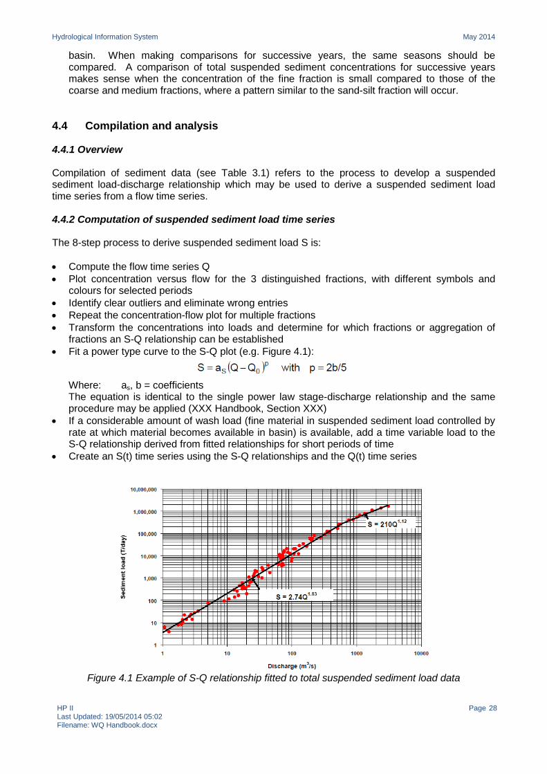
Hydrological Information System May 2014
HP II Last Updated: 19/05/2014 05:02 Filename: WQ Handbook.docx
Page 28
basin. When making comparisons for successive years, the same seasons should be compared. A comparison of total suspended sediment concentrations for successive years makes sense when the concentration of the fine fraction is small compared to those of the coarse and medium fractions, where a pattern similar to the sand-silt fraction will occur.
4.4 Compilation and analysis 4.4.1 Overview Compilation of sediment data (see Table 3.1) refers to the process to develop a suspended sediment load-discharge relationship which may be used to derive a suspended sediment load time series from a flow time series. 4.4.2 Computation of suspended sediment load time series The 8-step process to derive suspended sediment load S is: • Compute the flow time series Q • Plot concentration versus flow for the 3 distinguished fractions, with different symbols and
colours for selected periods • Identify clear outliers and eliminate wrong entries • Repeat the concentration-flow plot for multiple fractions • Transform the concentrations into loads and determine for which fractions or aggregation of
fractions an S-Q relationship can be established • Fit a power type curve to the S-Q plot (e.g. Figure 4.1):
Where: as, b = coefficients The equation is identical to the single power law stage-discharge relationship and the same procedure may be applied (XXX Handbook, Section XXX)
• If a considerable amount of wash load (fine material in suspended sediment load controlled by rate at which material becomes available in basin) is available, add a time variable load to the S-Q relationship derived from fitted relationships for short periods of time
• Create an S(t) time series using the S-Q relationships and the Q(t) time series
Figure 4.1 Example of S-Q relationship fitted to total suspended sediment load data

Hydrological Information System May 2014
HP II Last Updated: 19/05/2014 05:02 Filename: WQ Handbook.docx
Page 29
If more sediment sampling stations are available on the same river, a sediment balance should be made for river stretches to estimate the sedimentation or erosion rate in the reach. Such information may be compared with data on bed levels for the reach for the balance period, when available. If the river is entering a reservoir, which is regularly surveyed, a comparison should be made with the sedimentation rate in the reservoir. For this a percentage has to be added to the suspended load to account for bed load transport. The match will further be dependent on the trap efficiency of the reservoir.
Hydrological Information System May 2014
HP II Last Updated: 19/05/2014 05:02 Filename: WQ Handbook.docx
Page 30
5. Water Quality Data Processing and Analysis 5.1 Data entry 5.1.1 Overview Entry of water quality data to computer is primarily done in the laboratory where the water samples are analysed, though some parameters may have been measured in the field. For surface water data, data entry is carried out using e-SWIS, the data entry module of which replicates the SWDES software from HPI, and is referred to as eSWDES. For groundwater data, data entry is carried out using e-GEMS which has GWDES water quality functionality. Prior to analysis, two manual activities are essential: registration of receipt of the samples from the field or laboratory, and manual inspection of the forms and notebooks from the field, for complete information and obvious errors. Analysis of water quality samples should be completed within the allowed time period, and data entry (see Table 3.1) of analysis results should be done on the same day as the analysis, ready for primary validation also by the laboratory. 5.1.2 Entry of sample reference information Using the appropriate screen in e-SWIS or e-GEMS, the user enters information about when, where and how the water sample was collected and analysed. The sample reference information is entered for every water quality sample, and specifies: • Location (i.e. station code for flow gauging station, observation well or other sampling site) • Date/time information for the sampling • Laboratory conducting analysis and laboratory sample ID • Agency collecting the sample from the field and delivering it to the laboratory • Source of water sample (e.g. river, lake, rain, groundwater, etc) • Medium (e.g. water, suspended matter, solid, etc) and matrix (e.g. fresh water, brackish, salt,
effluent, etc) of water sample • Type of water sample (e.g. grab sample, time-composite, flow-composite, depth-integrated,
etc) • Depth at which the water sample was collected • Optional project or programme name, and type of monitoring (e.g. baseline, trend, flux,
surveillance, survey, etc) • Name of person collecting the sample in the field • Conditions of water and weather before and during the sampling which might influence the
sample • From sample specification form, the type of sample container (e.g. PE, Glass, Teflon, etc),
sample specification (i.e. type of analysis to be performed), volume of sample, sampling device (e.g. bottle, depth sampler, DO sampler, etc), preservation in field and treatment at laboratory.
The user is prompted should any of the entered data not be in the correct alphanumeric format or expected range. Each water quality sample is assigned a unique reference number. Many fields in the sample reference information will not change frequently, especially for those samples collected for routine monitoring. Therefore it is possible to save information about a specific sampling location as a template, which can be loaded when a new sample is created. Alternatively, many fields have a default value that is entered automatically when a new sample is created, and that the user may edit manually.
Hydrological Information System May 2014
HP II Last Updated: 19/05/2014 05:02 Filename: WQ Handbook.docx
Page 31
5.1.3 Entry of water quality data Having entered the sample reference information using the e-SWIS or e-GEMS software, the user next enters the analysis results for the sample. The user selects the correct laboratory or the correct sampling location, and the data entry screen shows all samples with laboratory sample ID and unique sample reference number, and date of collection and date of receipt. The user identifies the correct sample from the list and enters the analysis results, and field results (e.g. colour, odour, temperature, etc). The user is prompted should any of the entered data not be in the correct alphanumeric format or expected range. Each parameter has a pre-set maximum and minimum value, indicating the highest and lowest values that may be expected, as well as upper and lower warning limits, indicating unusually high or low values that may indicate suspect data. Values higher than the maximum limit set for a particular parameter cannot be entered. Each parameter also has a limit of detection for each analysis method. Values below the detection limit of the analysis method used for a particular parameter cannot be entered. Values below the detection limit therefore appear “missing”, and are known as censored data. For secondary validation (Section 5.3), the completeness of the data is important with respect to the analysis of time-dependent data because some techniques (e.g. statistical analysis) may not yield results unless the dataset is continuous dataset. The presence of censored data may make it difficult to summarise and compare datasets and may lead to biased estimates of means, variances, trends and other values. For analysis of censored data, a value of half the detection limit is used for “missing” values. Seven (indirect) parameters are automatically calculated based on entry of other (direct) parameters: Sodium Adsorption Ratio (SAR), Percent Sodium, Residual Sodium Carbonate (RSC), Calcium Ion (Ca2+), Magnesium Ion (Mg2+), Total Dissolved Solids (TDS), and Carbonate and Bicarbonate Ions (CO3
2- and HCO3-, respectively). Equations for these indirect parameters are
given in SW8-OM(I) Chapter 14.5.1 or GW8-OM(II) Chapter 1.5.1. 5.1.4 Entry of AQC data The HIS includes a system of quality control in laboratories based on Inter-laboratory Analytical Quality Control (AQC) exercises. The results of AQC exercise are important indicators of the laboratory performance. Participating laboratories use e-SWIS e-GEMS to enter their analytical results of the AQC samples, known as AQC data. The procedure is similar to that for entering water quality data for field samples (Section 5.1.3), except that the analysis results are entered through a bespoke AQC data entry screen in the software. 5.1.5 Entry of historical water quality data It is possible to enter or import historical water quality data into e-SWIS or e-GEMS, subject to the following conditions: • Units of parameters in the historical database must be converted to the prescribed units of the
e-SWIS or e-GEMS software before entry or import. • Indirect parameters in the historical database (e.g. SAR, RSC, etc) cannot be imported and the
calculation will be redone. The user should check that the historical and new values agree. • The method by which each historical parameter was analysed must be entered. If this is
different to the current method of analysis, the date the method was changed must also be recorded.
Hydrological Information System May 2014
HP II Last Updated: 19/05/2014 05:02 Filename: WQ Handbook.docx
Page 32
5.2 Primary validation 5.2.1 Overview Primary validation of water quality data is primarily done by the laboratory where the water samples are analysed and analysis results entered. For surface water data, data entry is carried out using e-SWIS, the data entry module of which replicates the SWDES software from HPI, and is referred to as eSWDES. For groundwater data, data entry is carried out using e-GEMS which has GWDES water quality functionality. The software performs several automatic validation checks for each sample. Prior to primary validation, the forms and notebooks from the field should be again inspected for complete information and obvious errors. Primary validation (see Table 3.1) of analysis results is required to be completed at Sub-Divisional office level within one week of data entry at the laboratory, ready for secondary validation by State offices. This time schedule ensures that any obvious problems (e.g. indicating an instrument malfunction, observer error, etc) are spotted at the earliest opportunity and resolved. Other problems may not become apparent until more data have been collected, and data can be viewed in a longer-term context during secondary validation. 5.2.2 Validation of water quality data Having entered the sample reference information using the e-SWIS or e-GEMS software, the user selects the correct laboratory or the correct sampling location, and the data validation screen shows all samples with laboratory sample ID and unique sample reference number, and date of collection and date of receipt. The user identifies the correct sample from the list. If a sample does not meet a specific validation check, the software will indicate that the analysis result is above or below the limit for that check. Automatic validation checks, described in SW8-OM(I) Chapter 15.2 or GW8-OM(II) Chapter 2, include: • Ion balance for cations and anions – the difference in the sum of major cations and the sum of
major anions should not exceed 10% (this value can be changed by the user) • Sodium and Chlorine ratio – the ratio should be between 0.8 and 1.2 • Conductivity (EC) and Total Dissolved Solids (TDS) ratio – the ratio should be between 0.55
and 0.9 • TDS calculated and TDS measured ratio – the ration should be between 1.0 and 1.2 • COD and BOD ratio – CODS values should always be higher than BOD values • Carbonate and pH relationship – carbonate should be zero for pH values below 8.3 The person conducting the primary validation should complete the “checked by” box on the data validation screen, as well as any comments (e.g. why a sample did not pass a particular validation check). The data entry and primary validation software also allow water quality data to be viewed graphically and compared with drinking water standards (i.e. Bureau of Indian Standards) and irrigation water standards. 5.3 Secondary validation 5.3.1 Overview Secondary validation of water quality data is primarily carried out at State DPCs. For surface water data, validation is carried out using e-SWIS, the validation module of which replicates the HYMOS software from HPI, and is referred to as eHYMOS. For groundwater data, validation is carried out using e-GEMS which has GEMS water quality functionality. Data may also be exported to Excel
Hydrological Information System May 2014
HP II Last Updated: 19/05/2014 05:02 Filename: WQ Handbook.docx
Page 33
for secondary validation. For the Hydrology Project, initial secondary validation (see Table 3.1) done at State level should be completed within one month of data entry. Some secondary validation (including comparison with CWC/CGWB/CPCB data) will not be possible until the end of the hydrological year when the entire year’s data can be reviewed in a long-term context, so data should be regarded as provisional approved data until then (e.g. for June data by the end of the hydrological year plus 3 months), after which data should be formally approved and made available for dissemination to external users. Secondary validation is largely concerned with detecting outliers, as described in SW8-OM(III) Chapter 8.2 and GW7-DM Chapter 2.9.2. An outlier is an observation that does not match the pattern of earlier observations. Outliers in water quality datasets may occur due to practical mistakes or instrumental failure in all aspects of water quality sampling and analysis: from sample collection, transport, storage, analysis or data entry. They may also result from transcription or data entry errors, or can be the result of instrument breakdowns, calibration problems or power failures. However, outliers may be an indication of a true change in the system under study, such as an accidental spill on a river stretch. The presence of one or more outliers within a data set may greatly influence any calculated statistics and yield biased results, so outliers should be identified, flagged and, if truly erroneous, possibly removed from a dataset. Screening water quality data, using tabular, graphical, computational and statistical validation techniques, is useful to identify and flag outliers. After identification of one or more outliers, a decision must be made about what to do with the data values. If an obvious mistake is detected, the correct data value may be entered, if available. Otherwise the outlier should be flagged (bit not removed from the database) and may need to be excluded from subsequent analysis, though it is also possible to leave the outlier in the dataset, and use statistical tests that are not so sensitive to outliers. Outliers should not be removed on the basis of statistical tests only as there is always a chance (the level of confidence of the test) that the test incorrectly declares a valid observation as outlier (e.g. water quality impacted by a rare event in the field, such as rain, flood, religious bathing, extra factory effluent, etc. 5.3.2 Control charts For each sampling location and parameter, historical data are used to calculate the mean value and upper/lower limits, which can be used as a guide for new data. A control chart shows a set of data values, together with the central line (mean of the data), warning limits (±2 standard deviations) and control limits (±3 standard deviations). New data may be plotted on the established control chart to identify any deviation in behaviour from the historical pattern. For a surface water quality monitoring programme with at least 6 observations a year, a period of 3 years should provide a meaningful historical data set. For a groundwater quality monitoring programme, only one or two observations a year are typically available, so would need a longer period to generate a representative control chart. If there are many years of historical data, annual or seasonal means can be used instead of individual data values. 5.3.3 Graphical analysis Graphical analysis of data is a useful first step to visually check if there are any outliers in a data set. Graphical analysis can be made by ranking the data (in increasing order) and preparing a probability plot or linear plot of ranked data. The highest and lowest values stand out from the rest of the data and may be outliers. Alternatively, trilinear Piper-diagrams or Stiff-diagrams may show deviating values as outlying points of deviating shapes, respectively (Figure 5.1; see GW7-DM Chapter 2.9.2) Suspected outliers should then be checked with statistical analysis (Section 5.3.4).
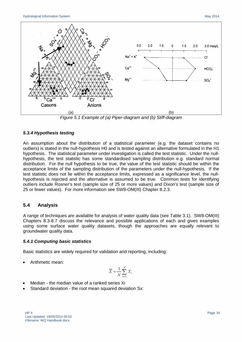
Hydrological Information System May 2014
HP II Last Updated: 19/05/2014 05:02 Filename: WQ Handbook.docx
Page 34
(a) (b) Figure 5.1 Example of (a) Piper-diagram and (b) Stiff-diagram
5.3.4 Hypothesis testing An assumption about the distribution of a statistical parameter (e.g. the dataset contains no outliers) is stated in the null-hypothesis H0 and is tested against an alternative formulated in the H1 hypothesis. The statistical parameter under investigation is called the test statistic. Under the null-hypothesis, the test statistic has some standardised sampling distribution e.g. standard normal distribution. For the null hypothesis to be true, the value of the test statistic should be within the acceptance limits of the sampling distribution of the parameters under the null-hypothesis. If the test statistic does not lie within the acceptance limits, expressed as a significance level, the null-hypothesis is rejected and the alternative is assumed to be true. Common tests for identifying outliers include Rosner’s test (sample size of 25 or more values) and Dixon’s test (sample size of 25 or fewer values). For more information see SW8-OM(III) Chapter 8.2.3. 5.4 Analysis A range of techniques are available for analysis of water quality data (see Table 3.1). SW8-OM(III) Chapters 8.3-8.7 discuss the relevance and possible applications of each and gives examples using some surface water quality datasets, though the approaches are equally relevant to groundwater quality data. 5.4.1 Computing basic statistics Basic statistics are widely required for validation and reporting, including: • Arithmetic mean:
• Median - the median value of a ranked series Xi • Standard deviation - the root mean squared deviation Sx:
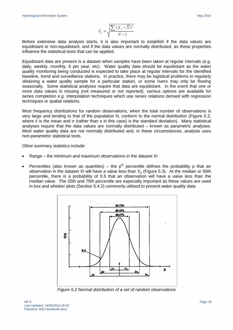
Hydrological Information System May 2014
HP II Last Updated: 19/05/2014 05:02 Filename: WQ Handbook.docx
Page 35
Before extensive data analysis starts, it is also important to establish if the data values are equidistant or non-equidistant, and if the data values are normally distributed, as these properties influence the statistical tests that can be applied. Equidistant data are present is a dataset when samples have been taken at regular intervals (e.g. daily, weekly, monthly, 6 per year, etc). Water quality data should be equidistant as the water quality monitoring being conducted is expected to take place at regular intervals for the identified baseline, trend and surveillance stations. In practice, there may be logistical problems in regularly obtaining a water quality sample for a particular station, or some rivers may only be flowing seasonally. Some statistical analyses require that data are equidistant. In the event that one or more data values is missing (not measured or not reported), various options are available for series completion e.g. interpolation techniques which use series relations derived with regression techniques or spatial relations. Most frequency distributions for random observations, when the total number of observations is very large and tending to that of the population N, conform to the normal distribution (Figure 5.2, where x� is the mean and σ (rather than s in this case) is the standard deviation). Many statistical analyses require that the data values are normally distributed – known as parametric analyses. Most water quality data are not normally distributed and, in these circumstances, analysis uses non-parametric statistical tests. Other summary statistics include: • Range – the minimum and maximum observations in the dataset Xi • Percentiles (also known as quantiles) – the pth percentile defines the probability p that an
observation in the dataset Xi will have a value less than Xp (Figure 5.3). At the median or 50th percentile, there is a probability of 0.5 that an observation will have a value less than the median value. The 25th and 75th percentile are especially important as these values are used in box and whisker plots (Section 5.4.2) commonly utilised to present water quality data.
Figure 5.2 Normal distribution of a set of random observations
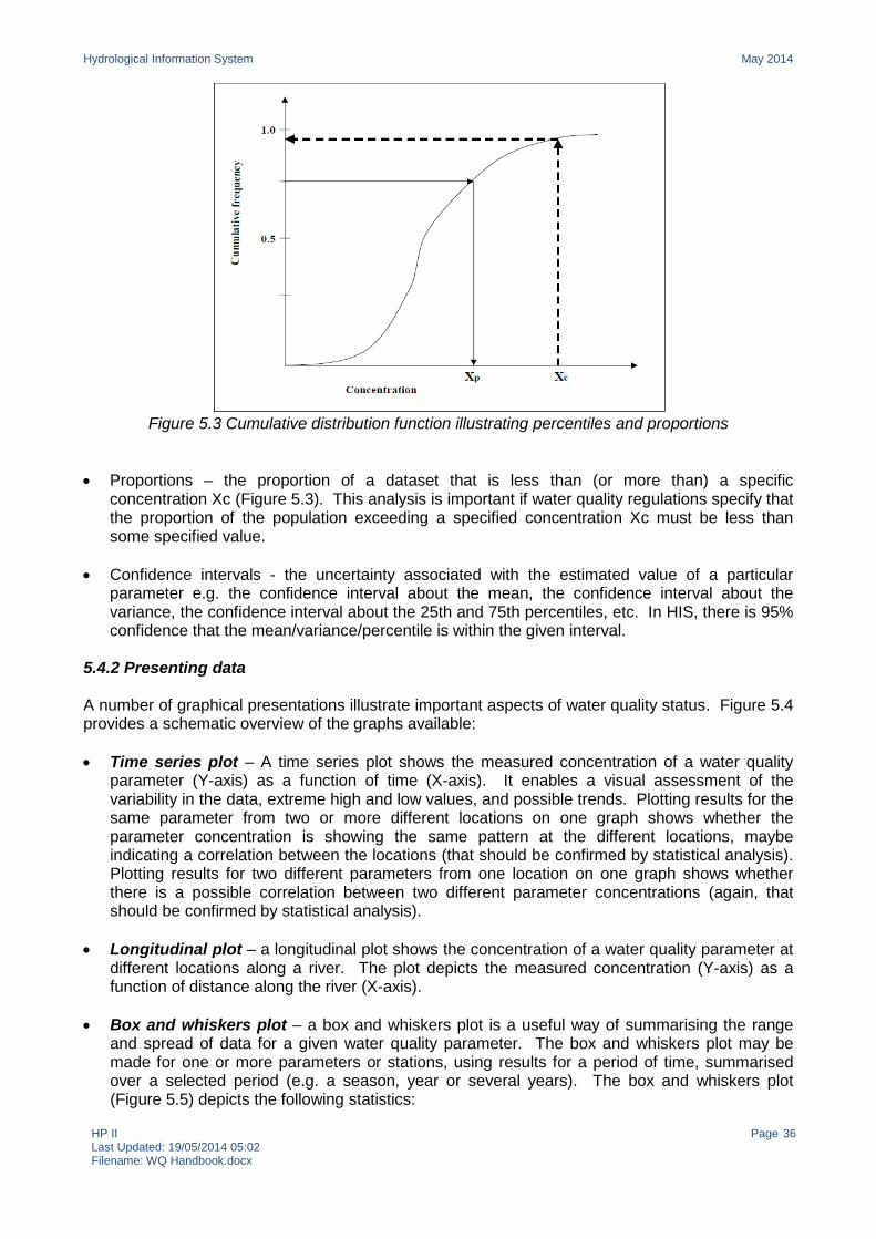
Hydrological Information System May 2014
HP II Last Updated: 19/05/2014 05:02 Filename: WQ Handbook.docx
Page 36
Figure 5.3 Cumulative distribution function illustrating percentiles and proportions
• Proportions – the proportion of a dataset that is less than (or more than) a specific
concentration Xc (Figure 5.3). This analysis is important if water quality regulations specify that the proportion of the population exceeding a specified concentration Xc must be less than some specified value.
• Confidence intervals - the uncertainty associated with the estimated value of a particular
parameter e.g. the confidence interval about the mean, the confidence interval about the variance, the confidence interval about the 25th and 75th percentiles, etc. In HIS, there is 95% confidence that the mean/variance/percentile is within the given interval.
5.4.2 Presenting data A number of graphical presentations illustrate important aspects of water quality status. Figure 5.4 provides a schematic overview of the graphs available: • Time series plot – A time series plot shows the measured concentration of a water quality
parameter (Y-axis) as a function of time (X-axis). It enables a visual assessment of the variability in the data, extreme high and low values, and possible trends. Plotting results for the same parameter from two or more different locations on one graph shows whether the parameter concentration is showing the same pattern at the different locations, maybe indicating a correlation between the locations (that should be confirmed by statistical analysis). Plotting results for two different parameters from one location on one graph shows whether there is a possible correlation between two different parameter concentrations (again, that should be confirmed by statistical analysis).
• Longitudinal plot – a longitudinal plot shows the concentration of a water quality parameter at
different locations along a river. The plot depicts the measured concentration (Y-axis) as a function of distance along the river (X-axis).
• Box and whiskers plot – a box and whiskers plot is a useful way of summarising the range
and spread of data for a given water quality parameter. The box and whiskers plot may be made for one or more parameters or stations, using results for a period of time, summarised over a selected period (e.g. a season, year or several years). The box and whiskers plot (Figure 5.5) depicts the following statistics:
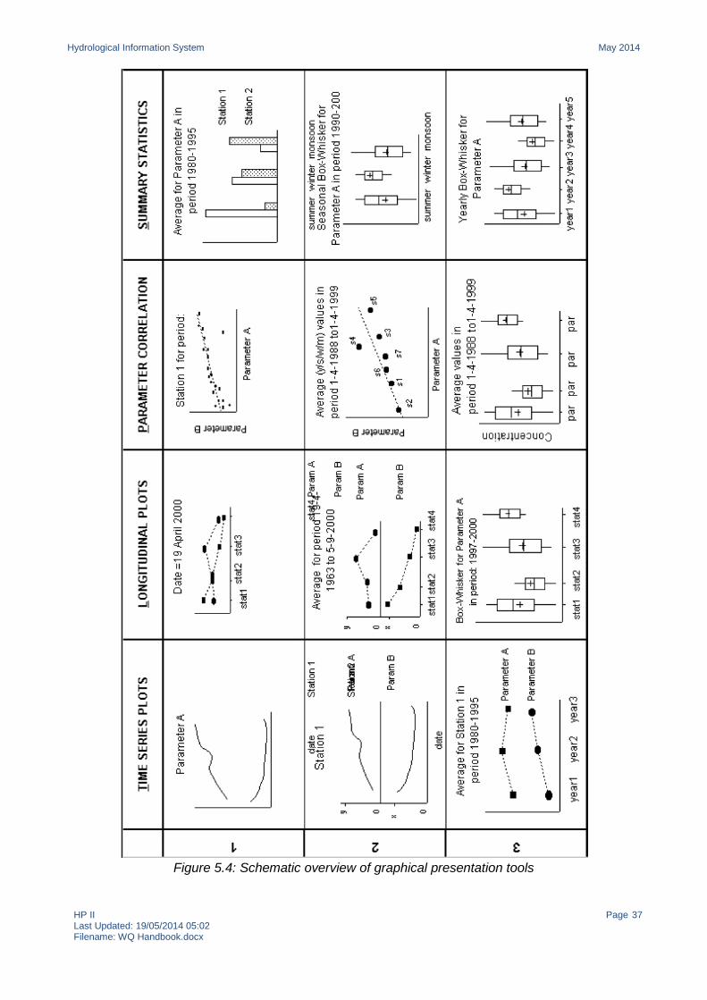
Hydrological Information System May 2014
HP II Last Updated: 19/05/2014 05:02 Filename: WQ Handbook.docx
Page 37
Figure 5.4: Schematic overview of graphical presentation tools
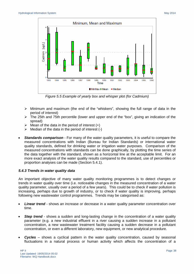
Hydrological Information System May 2014
HP II Last Updated: 19/05/2014 05:02 Filename: WQ Handbook.docx
Page 38
Figure 5.5 Example of yearly box and whisper plot (for Cadmium)
Minimum and maximum (the end of the “whiskers”, showing the full range of data in the
period of interest) The 25th and 75th percentile (lower and upper end of the “box”, giving an indication of the
spread) Mean of the data in the period of interest (+) Median of the data in the period of interest (-)
• Standards comparison - For many of the water quality parameters, it is useful to compare the
measured concentrations with Indian (Bureau for Indian Standards) or international water quality standards, defined for drinking water or irrigation water purposes. Comparison of the measured concentrations with standards can be done graphically, by plotting the time series of the data together with the standard, shown as a horizontal line at the acceptable limit. For an more exact analysis of the water quality results compared to the standard, use of percentiles or proportion analyses can be made (Section 5.4.1).
5.4.3 Trends in water quality data An important objective of many water quality monitoring programmes is to detect changes or trends in water quality over time (i.e. noticeable changes in the measured concentration of a water quality parameter, usually over a period of a few years). This could be to check if water pollution is increasing, perhaps due to growth of industry, or to check if water quality is improving, perhaps following new wastewater control programmes. Trends may be categorised as: • Linear trend - shows an increase or decrease in a water quality parameter concentration over
time. • Step trend - shows a sudden and long-lasting change in the concentration of a water quality
parameter (e.g. a new industrial effluent in a river causing a sudden increase in a pollutant concentration, a new wastewater treatment facility causing a sudden decrease in a pollutant concentration, or even a different laboratory, new equipment, or new analytical procedure.
• Cycles – shows a cyclical pattern in the water quality concentration, caused by seasonal
fluctuations in a natural process or human activity which affects the concentration of a
Hydrological Information System May 2014
HP II Last Updated: 19/05/2014 05:02 Filename: WQ Handbook.docx
Page 39
particular parameter. Cycles are not real trends because they do not indicate a long-term change, and special care must be taken in analysing trends if cycles are present in the dataset.
Time series analysis and hypothesis testing (e.g. Seasonal Kendall Slope test, Wilcoxon Signed Rank test, Student’s t-test, Wilcoxon Ranked Sum test, Wilcoxon W-test) may be used to investigate the trend in a water quality data series. For more information see SW8-OM(III) Chapters 8.6 and 8.7.
Hydrological Information System May 2014
HP II Last Updated: 19/05/2014 05:02 Filename: WQ Handbook.docx
Page 40
6. Data Dissemination and Publication 6.1 Sediment and water quality products The traditional primary visible output of hydrological data archives is published reports, usually in the form of annual hydrological and groundwater yearbooks. However, this is not generally the most convenient format of sediment and water quality data for data users who often require long-term records for a single station or a group of stations i.e. data by station rather than by year. For data users in the past, this necessitated the collation of data from a set of annual reports and the keying in of the data for the required analysis. In many countries, recent advances in IT, combined with well-established links between data suppliers and data users, mean that annual reports are no longer published in print, with the same information being provided online, and data requests met with a rapid and bespoke response. A further consequence is that data suppliers have more time to focus on data analysis, periodic reports and short-term operational reports of interest to key data users e.g. reports on major storm of flood events that may have water quality implications, real-time water quality data for pollution monitoring, water quality bulletins for agricultural, fisheries and recreation users, etc. A combination of digital and hardcopy hydrological products and online dissemination provide an effective means of demonstrating the capability of the HIS, in particular: • Providing information on availability of data for use in planning and design, and making
reporting and use of data more efficient by reducing the amount of published data and cost of annual reports
• Advertising the work of the HIS and its capability, and to create interest and awareness amongst potential data users
• Providing tangible evidence to policymakers of a return on substantial investment • Providing feedback to data producers, and acknowledging the contribution of observers and
co-operating agencies • Providing a clear incentive to keep archives up to data and a focus for an annual hydrometric
audit Hence, the long-term goal of the HIS is web-based dissemination of user guidance and station metadata (additional datasets that include items that could assist users of the data to understand the data, their accuracy and any major influencing factor), which is usefully complemented by the publication of catalogues or registers of hydrometric stations (e.g. Marsh & Hannaford, 2008) and occasional reports, and by a dedicated enquiry and data retrieval service. 6.2 Annual reports 6.2.1 Hydrological and groundwater yearbooks Hydrological and groundwater yearbooks should report over the hydrological year from 1 June to 31 May. The hydrological year corresponds to a complete cycle of replenishment and depletion, so it is appropriate to report on that basis rather than over the calendar year. Annual hydro-meteorological and surface water quantity and water quality information may be presented in a single combined hydrological report (see Water Level, Stage-Discharge and Flow Handbook, Section 7 for surface water reporting), or annual hydro-meteorological and groundwater levels and water quality information (see Groundwater Handbook, Section 6 for groundwater reporting) may be presented in a single combined groundwater report. Annual reports are produced at the State DPC and should be published within 12 months of the end of the hydrological year covered. SW8-
Hydrological Information System May 2014
HP II Last Updated: 19/05/2014 05:02 Filename: WQ Handbook.docx
Page 41
OM(III) Annex I and GW8-OM(V) present templates for Surface Water and Groundwater Yearbooks published at State level. Sediment reporting The sediment element of hydrological yearbooks should provide a summary of sediment loads for the report year in terms of distribution and time. Details of the observational network and data availability should be included, and it should make comparisons with long-term statistics. Typical contents of an annual report with respect to sediment transport include: • Introduction - The report introduction may change little from year to year, describing the
administrative organisation of the sediment monitoring networks and associated surface water networks, including any agencies contributing to the included data. The report should explain how the work is linked with other agencies collecting or using sediment data including CWC and CPCB. It should also set out how data may be requested and under what terms and conditions they are supplied.
• Observational network for sediment sampling: Network layout and adaptations in the report year – presenting network particulars as
tables and graphs in line with those used for flow data (Water level, Stage-Discharge and Flow Handbook, Section 7.2.1).
Monitoring and processing - with respect to sediment sampling, describing the monitoring procedures and equipment, and any changes that have taken place, and any other information to aid interpretation the sediment loads e.g. existence of bank erosion and mining of the river bed upstream of the measuring site, topographical and land use practices, etc. The description should present a clear picture of the site conditions and sediment sources.
Data collection in the report year – outlining the data validation and applied computational procedures used for arriving at the sediment load values for different time intervals (10-day, monthly and annual).
• Sediment transport: Sediment loads in the report year - presenting 10-day, monthly and annual total suspended
sediment loads for selected stations and the annual total loads for all stations. Presented data should be based on S-Q relationships (Section 4.4.2) derived for the station and valid for that particular year or part of the year. To show the contributions of the coarse, medium and fine fractions to the total load the individual 10-day, monthly and annual loads or average concentrations may also be given.
Sediment loads in comparison to the historical records - showing the sediment loads for the current year, in relation to the historical data. The current year should be displayed in frequency curves derived from the historical record, based on 10-day values.
• Trends in sediment loads - when records of sufficient length are available, showing the long-
term development of sediment loads for the report year and for the seasons separately. Information should be presented on possible causes of any changes in the S-Q relationships e.g. existence of bank erosion and mining of the river bed upstream of the measuring site, different measuring equipment and/or practices, etc. This may be important when interpreting current data in a historical context.
• Interpretation - of various sediment transport statistics presented in the hydrological yearbook. Water quality reporting The water quality element of hydrological or groundwater yearbooks should provide a summary of water quality changes for the report year. Details of the observational network and data availability
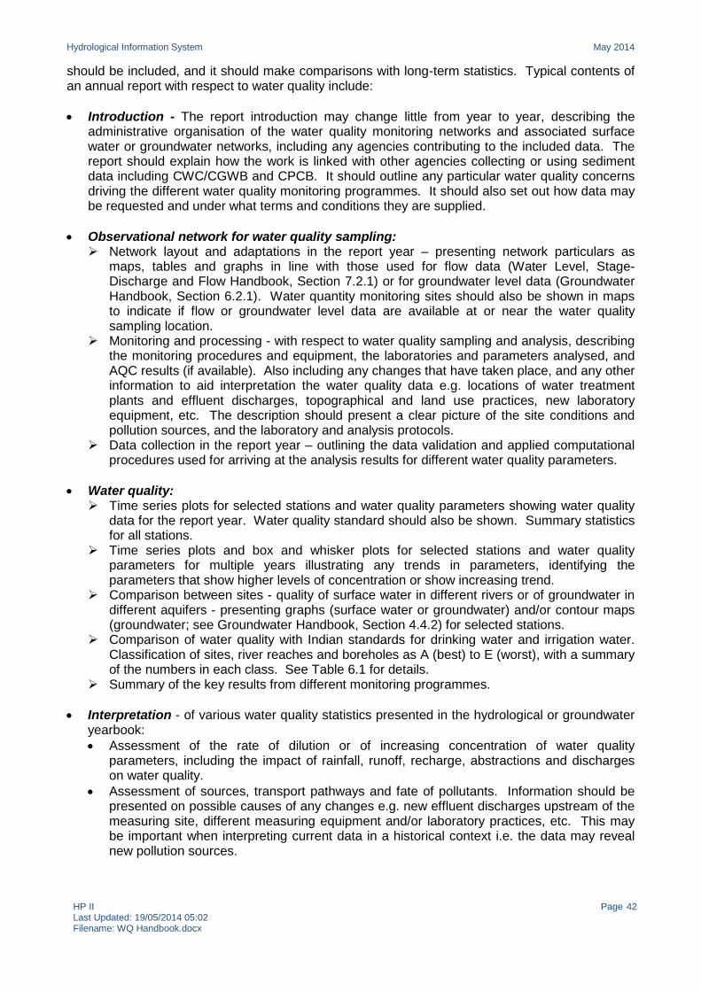
Hydrological Information System May 2014
HP II Last Updated: 19/05/2014 05:02 Filename: WQ Handbook.docx
Page 42
should be included, and it should make comparisons with long-term statistics. Typical contents of an annual report with respect to water quality include: • Introduction - The report introduction may change little from year to year, describing the
administrative organisation of the water quality monitoring networks and associated surface water or groundwater networks, including any agencies contributing to the included data. The report should explain how the work is linked with other agencies collecting or using sediment data including CWC/CGWB and CPCB. It should outline any particular water quality concerns driving the different water quality monitoring programmes. It should also set out how data may be requested and under what terms and conditions they are supplied.
• Observational network for water quality sampling: Network layout and adaptations in the report year – presenting network particulars as
maps, tables and graphs in line with those used for flow data (Water Level, Stage-Discharge and Flow Handbook, Section 7.2.1) or for groundwater level data (Groundwater Handbook, Section 6.2.1). Water quantity monitoring sites should also be shown in maps to indicate if flow or groundwater level data are available at or near the water quality sampling location.
Monitoring and processing - with respect to water quality sampling and analysis, describing the monitoring procedures and equipment, the laboratories and parameters analysed, and AQC results (if available). Also including any changes that have taken place, and any other information to aid interpretation the water quality data e.g. locations of water treatment plants and effluent discharges, topographical and land use practices, new laboratory equipment, etc. The description should present a clear picture of the site conditions and pollution sources, and the laboratory and analysis protocols.
Data collection in the report year – outlining the data validation and applied computational procedures used for arriving at the analysis results for different water quality parameters.
• Water quality: Time series plots for selected stations and water quality parameters showing water quality
data for the report year. Water quality standard should also be shown. Summary statistics for all stations.
Time series plots and box and whisker plots for selected stations and water quality parameters for multiple years illustrating any trends in parameters, identifying the parameters that show higher levels of concentration or show increasing trend.
Comparison between sites - quality of surface water in different rivers or of groundwater in different aquifers - presenting graphs (surface water or groundwater) and/or contour maps (groundwater; see Groundwater Handbook, Section 4.4.2) for selected stations.
Comparison of water quality with Indian standards for drinking water and irrigation water. Classification of sites, river reaches and boreholes as A (best) to E (worst), with a summary of the numbers in each class. See Table 6.1 for details.
Summary of the key results from different monitoring programmes. • Interpretation - of various water quality statistics presented in the hydrological or groundwater
yearbook: • Assessment of the rate of dilution or of increasing concentration of water quality
parameters, including the impact of rainfall, runoff, recharge, abstractions and discharges on water quality.
• Assessment of sources, transport pathways and fate of pollutants. Information should be presented on possible causes of any changes e.g. new effluent discharges upstream of the measuring site, different measuring equipment and/or laboratory practices, etc. This may be important when interpreting current data in a historical context i.e. the data may reveal new pollution sources.
Hydrological Information System May 2014
HP II Last Updated: 19/05/2014 05:02 Filename: WQ Handbook.docx
Page 43
Table 6.1 Water quality criteria for various uses of fresh water Designated best use Class Criteria Drinking water source without conventional treatment but after disinfection
A Total coliform organisms MPN/100mL 50 or less pH between 6.5 and 8.5 DO 6 mg/L or more BOD 2 mg/L or less
Outdoor bathing (organised) B Total coliform organisms MPN/100mL 500 or less pH between 6.5 and 8.5 DO 5 mg/L or more BOD 3 mg/L or less
Drinking water source with conventional treatment followed by disinfection
C Total coliform organisms MPN/ 100mL 5000 or less pH between 6 and 9 DO 4 mg/L or more BOD 3 mg/L or less
Propagation of wild life, fisheries D pH between 6.5 and 8.5 DO 4 mg/L or more Free ammonia (as N) 1.2 mg/L or less
Irrigation, industrial cooling, controlled waste disposal
E pH between 6.0 and 8.5 EC less than 2250 micro mhos/cm SAR less than 26 Boron less than 2mg/L
6.2.2 Annual hydrological reviews Shorter than hydrological yearbooks, annual reviews of the hydrological year provide users with published assessments of the key elements of the hydrological cycle. Hence, the reports combine hydro-meteorological, surface water, ground water with, where appropriate, sediment and water quality data. Annual reviews are produced at the State DPC and should be published within 12 months of the end of the hydrological year covered. For an example, see www.ceh.ac.uk/data/nrfa/nhmp/annual_review.html. 6.3 Periodic reports 6.3.1 Metadata catalogues Periodic surface water reports of flow, sediment and water quality metadata and time series statistics, or of groundwater level and water quality metadata and time series statistics, may be published by the State DPC at 5-year or 10-year intervals. The reports should incorporate spatial as well as temporal analysis and provide statistical summaries in tabular and graphical to make the information accessible and interesting to data users. For more information, see Water Level, Stage-Discharge and Flow Handbook, Section 7.3.1) or for groundwater level data (Groundwater Handbook, Section 6.3.1. 6.3.2 Monthly hydrological summaries Routine monthly reports and statistics on the current state hydrological situation, including assessments of rainfall, snow (where relevant), evaporation, river flow, groundwater and reservoir stocks, provide users with a snapshot of the current situation and its historical context, and the
Hydrological Information System May 2014
HP II Last Updated: 19/05/2014 05:02 Filename: WQ Handbook.docx
Page 44
future outlook. Such information may provide a vital input for planning domestic or industrial water supply, agricultural planning, hydropower and other water use sectors, and could be expanded to include sediment and water quality data if appropriate. Monthly summaries are produced at the State DPC and should be published within 10 working days of the month covered. For an example, see www.ceh.ac.uk/data/NRFA/nhmp/monthly_hs.html. 6.4 Dissemination to hydrological data users Final (approved) sediment and water quality datasets are provided by Central/State hydrometric agencies on a request basis. The online HIS data catalogues in e-SWIS and e-GEMS which show the availability of fully validated (approved) data, supports hydrometric agencies in disseminating their data, and also helps hydrological data users to search available data and formulate their data requests and the formats required and direct them to the appropriate agency. The more comprehensive the information a data catalogue provides, the easier for users to identify the monitoring stations of interest to them, and be aware of any limitations to exploiting the data effectively. Users should be informed of the quality of any data supplied indicated by the data flag (e.g. observed, estimated, suspect, etc). There may be a charge for data which is the product of significant investment in equipment and staff time. Data requests from users should be processed promptly: at least 95% of queries should be dealt with within 5 working days, and the remaining up to 5% of queries, which should be the more complex ones, within 20 working days.
Hydrological Information System May 2014
HP II Last Updated: 19/05/2014 05:02 Filename: WQ Handbook.docx
Page 45
References Marsh, T.J. 2002. Capitalising on river flow data to meet changing national needs — a UK perspective. Flow Measurement and Instrumentation 13, 291–298. Marsh, T.J. & Hannaford, J. (eds). 2008. UK Hydrometric Register. Centre for Ecology & Hydrology, Wallingford, UK. www.ceh.ac.uk/products/publications/documents/hydrometricregister_final_withcovers.pdf World Meteorological Organisation. 2008. Guide to Hydrological Practices Volume I: Hydrology – From Measurement to Hydrological Information. Report No 168. www.whycos.org/hwrp/guide/ World Meteorological Organisation. 2009. Guide to Hydrological Practices Volume II: Management of Water Resources and Application of Hydrological Practices. Report No 168. www.whycos.org/hwrp/guide/
Hydrological Information System May 2014
HP II Last Updated: 19/05/2014 05:02 Filename: WQ Handbook.docx
Page 46
Annex I States and Agencies participating in the Hydrology Project Phase I (1996-2003) Phase II (2006-2014) States States Andhra Pradesh Andhra Pradesh Chhattisgarh Chhattisgarh Goa Gujurat Gujurat Himachal Pradesh Kerala Kerala Karnataka Karnataka Madhya Pradesh Madhya Pradesh Maharastra Maharastra Orissa Orissa Pondicherry Punjab Tamil Nadu Tamil Nadu Agencies Agencies Bhakra-Beas Management Board (BBMB) Central Ground Water Board (CGWB) Central Ground Water Board (CGWB) Central Pollution Control Board (CPCB) Central Water and Power Research Station
(CWPRS) Central Water and Power Research Station
(CWPRS) Central Water Commission (CWC) Central Water Commission (CWC) Indian Meteorological Department (IMD) Indian Meteorological Department (IMD) Ministry of Water Resources (MoWR) Ministry of Water Resources (MoWR) National Institute of Hydrology (NIH) National Institute of Hydrology (NIH)
Hydrological Information System May 2014
HP II Last Updated: 19/05/2014 05:02 Filename: WQ Handbook.docx
Page 47
Annex II Summary of Distribution of Hard Copy of HPI HIS Manual Surface Water
Volume Manual Part Training State
DSC State DPC
Div DPC
Sub-Div DPC
Station/ Lab
1 HIS Design + + + + + Field I Job description + + + + +
II ToR for HDUG + + + + III Data needs assessment + + + +
Reference + + + 2 Sampling Principles
Design + + + + + Reference + + +
3 Hydro-meteorology
Design + + + + + Field I Network design & site
selection + + + + +
II SRG operation & maintenance
+ + + + + 1 SRG
III ARG/TBR/SRG operation & maintenance
+ + + + + 1 ARG
IV FCS operation & maintenance
+ + + + + 1 FCS
V Field inspections, audits, maintenance & calibration
+ + + + +
Reference + + + 4 Hydrometry Design + + + + +
Field I Network design & site selection
+ + + + +
II River stage observation + + + + + + III Float measurements + + + + + + IV Current meter gauging + + + + + + V Field application of ADCP + + + (+) + (+) VI Slope-are method + + + + + + VII Field inspection & audits + + + + + VIII Maintenance & calibration + + + + +
Reference + + + 5 Sediment Transport
Design + + + + + Field + + + + + + Reference + + +
6 WQ Sampling
Design + + + + + Field + + + + + +
7 WQ Analysis Design + + + + Operation + + + +
8 Data Processing & Analysis
Operation I Data entry & primary validation
+ + + + +
II Secondary validation + + + + III Final processing & analysis + + + IV Data management + + + + +
9 Data Transfer, Storage & Dissemination
Design + + + Operation + + +
10 SW Protocols
Operation + + + + + + Forms + + + + + +

Hydrological Information System May 2014
HP II Last Updated: 19/05/2014 05:02 Filename: WQ Handbook.docx
Page 48
Annex III Summary of Distribution of Hard Copy of HPI HIS Manual Groundwater
Volume Manual Part Training State
DSC State DPC
Div DPC
Sub-Div DPC
Station/ Lab
1 HIS Design + + + + + Field I Job description + + + + +
II ToR for HDUG + + + + III Data needs assessment + + + +
Reference + + + 2 Sampling Principles
Design + + + + + Reference + + +
3 Hydro-meteorology
Design + + + + + Field I Network design & site
selection + + + + +
II SRG operation & maintenance
+ + + + + 1 SRG
III ARG/TBR/SRG operation & maintenance
+ + + + + 1 ARG
IV FCS operation & maintenance
+ + + + + 1 FCS
V Field inspections, audits, maintenance & calibration
+ + + + +
Reference + + + 4 Geo-Hydrology
Design + + + + + Field I Network design & site
selection + + + + +
II Drilling litho-specific piezometers
+ + + + + +
III Aquifer tests + + + + + + IV DWLR testing + + + + + + V Reduced levels of wells + + + + + + VI Manual water level collection
+ + + + + +
VII DWLR water level collection
+ + + + + +
VIII Inspection & maintenance + + + + + + Reference + + +
5 GIS Operation + + + + + + 6 WQ Sampling
Design + + + + + Field + + + + + +
7 WQ Analysis Design + + + + Operation + + + +
8 Data Processing & Analysis
Operation I Data entry & data validation – water level
+ + + + +
II Data entry and primary validation – water quality
+ + + + + +
III Data processing & analysis + + + + + IV GW resource assessment + + + + + IV GW yearbook + + + + +
9 Data Transfer, Storage & Dissemination
Design + + + Operation + + +
10 HIS Activities - GW Domain
Operation + + + + + +


