Finance and Economics Discussion Series Divisions of Research & Statistics and Monetary Affairs Federal Reserve Board, Washington, D.C. Credit Default Swap Spreads and Variance Risk Premia Hao Wang, Hao Zhou, and Yi Zhou 2011-02 NOTE: Staff working papers in the Finance and Economics Discussion Series (FEDS) are preliminary materials circulated to stimulate discussion and critical comment. The analysis and conclusions set forth are those of the authors and do not indicate concurrence by other members of the research staff or the Board of Governors. References in publications to the Finance and Economics Discussion Series (other than acknowledgement) should be cleared with the author(s) to protect the tentative character of these papers.
Transcript
Finance and Economics Discussion SeriesDivisions of Research & Statistics and Monetary Affairs
Federal Reserve Board, Washington, D.C.
Credit Default Swap Spreads and Variance Risk Premia
Hao Wang, Hao Zhou, and Yi Zhou
2011-02
NOTE: Staff working papers in the Finance and Economics Discussion Series (FEDS) are preliminarymaterials circulated to stimulate discussion and critical comment. The analysis and conclusions set forthare those of the authors and do not indicate concurrence by other members of the research staff or theBoard of Governors. References in publications to the Finance and Economics Discussion Series (other thanacknowledgement) should be cleared with the author(s) to protect the tentative character of these papers.
Credit Default Swap Spreads and Variance Risk Premia∗
Hao Wang† Hao Zhou‡ Yi Zhou§
First Draft: August 2009This Version: October 2010
Abstract
We find that firm-level variance risk premium, estimated as the difference between
option-implied and expected variances, has a prominent explanatory power for credit
spreads in the presence of market- and firm-level risk control variables identified in
the existing literature. Such a predictability complements that of the leading state
variable—leverage ratio—and strengthens significantly with lower firm credit rating,
longer credit contract maturity, and model-free implied variance. We provide further
evidence that: (1) variance risk premium has a cleaner systematic component and
Granger-causes implied and expected variances, (2) the cross-section of firms’ variance
risk premia seem to price the market variance risk correctly, and (3) a structural
model with stochastic volatility can reproduce the predictability pattern of variance
∗We would like to thank Turan Bali, Michael Brennan, Darrell Duffie, Louis Ederington, Robert Geske,Bing Han, Jean Helwege, Robert Jarrow, George Jiang, William Megginson, George Tauchen, Marliese Uhrig-Homburg, Jan Werner, Yelena Larkin, Liuren Wu, Yuhang Xing, Hong Yan; seminar participants at TsinghuaUniversity, University of Oklahoma, University of Texas at Dallas, University of South Carolina, BaruchCollege; and conference participants at FDIC, FIRS, CICF, EFA, and FMA for helpful discussions. Theauthors acknowledge the generous financial support from Global Association of Risk Professionals (GARP)and Center for Hedge Fund Research (CHFR) at Imperial College London.†Tsinghua University, School of Economics and Management, 318 Weilun Building, Beijing 100084, China,
E-mail: [email protected], Tel: 86 10-62797482.‡Corresponding Author: Federal Reserve Board, Risk Analysis Section, Washington, DC 20551, USA,
E-mail: [email protected], Tel: 1 202-452-3360.§University of Oklahoma, Michael F. Price College of Business, Finance Division, 307 West Brooks Street,
Adams Hall 250, Norman, OK 73069, USA, E-mail: [email protected], Tel: 1 405-325-1135.
Credit Default Swap Spreads and Variance Risk Premia
Abstract
We find that firm-level variance risk premium, estimated as the difference between option-
implied and expected variances, has a prominent explanatory power for credit spreads in the
presence of market- and firm-level risk control variables identified in the existing literature.
Such a predictability complements that of the leading state variable—leverage ratio—and
strengthens significantly with lower firm credit rating, longer credit contract maturity, and
model-free implied variance. We provide further evidence that: (1) variance risk premium has
a cleaner systematic component and Granger-causes implied and expected variances, (2) the
cross-section of firms’ variance risk premia seem to price the market variance risk correctly,
and (3) a structural model with stochastic volatility can reproduce the predictability pattern
Dufresne, and Goldstein, 2009; Chen, 2009), but focuses on providing cross-sectional evidence
of individual firms. We also find that VRP complements leverage ratio, which has been shown
as a leading explanatory variable for credit spreads (Collin-Dufresne and Goldstein, 2001).
1
Importantly, this firm-level VRP measure crowds out the popular market VRP (and VIX)
that has been shown as a strong predictor for aggregate credit spread indices (Zhou, 2009;
Buraschi, Trojani, and Vedolin, 2009). Such a predictive power turns out to be greater for
speculative-grade credit spreads, longer CDS contract maturities, and VRP constructed from
model-free option-implied variances.
Previous research seems to suggest that implied variance is informatively more efficient
than realized variance in predicting credit spreads (Cao, Yu, and Zhong, 2008; Berndt, Look-
man, and Obreja, 2006; Carr and Wu, 2008a). However, by decomposing the implied variance
into VRP and expected variance, we find that VRP can substitute most of the explaining
power of implied variance, especially for lower frequencies of monthly and quarterly relative
to weekly. We also present evidence that the first principle component of VRP across all
firms explains 78 percent of the total variation, while that of implied variance only explains
54 percent and expected variance only 57 percent. Finally we show that, at aggregate level,
VRP Granger causes implied and expected variances, but not vise versa. These additional
findings imply that VRP may be an ideal measure of firms’ exposures to a systematic vari-
ance risk factor, and the economic interpretation of implied variance in explaining credit
spread could largely reside on VRPs that are exposed to such a macroeconomic uncertainty
risk.
To further corroborate the interpretation that firm VRPs are exposures to systematic
uncertainty risk, we provide two additional justifications. In the first exercise, we run a
two-pass regression of individual firms’ VRP on the market VRP. The second stage cross-
sectional regression obtains an R2 of 14 percent and the estimated market VRP is 1.17
compared to the observed one of 1.20. In contrast, a similar exercise with firm equity returns
obtains an R2 of 0.00 and estimated market return of 0.03 compared to observed one of 0.46.
This result suggests that the cross-section of individual firms’ VRPs may correctly price a
systematic variance or economic uncertainty risk factor. In another exercise, we simulate
from a structural model with stochastic volatility, and find that VRP can indeed provide
additional explaining power for a representative firm’s credit spreads, even with the control of
true leverage ratio. On the contrary, the Merton model without stochastic volatility cannot
2
reproduce such a stylized pattern found in our empirical exercise.
Our work is related to the recent effort on explaining individual firms’ credit spreads
from several innovative angles. Campbell and Taksler (2003) find that the increases in bond
spreads can be explained by the upward trend in idiosyncratic equity volatility. Cremers,
Driessen, Maenhout, and Weinbaum (2008) rely on option-implied jump risk measure to
interpret the cross-sectional variations in default risk premia. Ericsson, Jacobs, and Oviedo
(2004); Ericsson, Reneby, and Wang (2006) exploit credit derivatives in explaining credit
spreads and evaluating structural models. Our study shares with the same spirit in terms
of risk-based explanations but emphasizes on using VRP as a novel tool to isolate the firm’s
exposure to systematic variance risk from its idiosyncratic counterpart. This provides an eco-
nomic interpretation for the superior predictive power of implied variance on credit spreads,
and point to a clear direction for improving the structural credit risk modeling—by incor-
porating a systematic variance risk factor.
The rest of the paper will be organized as the following: Section 2 introduces the variance
risk premium measure and our empirical methodology; followed by a description of data
sources and summary statistics in Section 3; then Section 4 presents empirical findings of
variance risk premium with respect to predicting credit spreads and discusses some economic
interpretations; and Section 5 concludes.
2 Variance Risk Premia and Empirical Methodology
In this section, we introduce the concept of variance risk premium (VRP) for individual
firms, following the recent literature in defining the market VRP as a difference between the
model-free implied variance and forecasted realized variance. Then we outline our empirical
strategy for explaining the credit default swap (CDS) spreads of individual firms, using
such a firm specific VRP variable, together with other established market and firm control
variables—noticeably the firm leverage ratio and risk-free rate.
3
2.1 Constructing the VRP Measure for Individual Firms
To construct the benchmark measure of firm VRP, we compute the model-free implied vari-
ances from the OptionMetrics data of the individual firms’ equity option prices and the
forecasted realized variances from high-frequency stock returns of individual companies.
Following Britten-Jones and Neuberger (2000), we apply Cox, Ross, and Rubinstein
(1979) or CRR binomial lattice model to translate the OptionMetrics prices of American
call options of different maturities and moneyness into implied volatilities. By fitting a
smooth cubic splines function to the implied volatilities, we compute the term structure of
implied volatilities at various strikes for call options of T -maturity. Then the term structure
of implied volatilities are translated back into the term structure of call prices at various
strikes using the CRR model. Note that such a procedure is not model-dependent, as the
CRR model serves merely as a mapping device between option prices and implied volatilities
(Jiang and Tian, 2005).
With the term structure of call option prices, we compute risk-neutral or model-free
implied variance by summing the following functional form over a spectrum of densely pop-
ulated strike prices:
IVi,t ≡ EQt [Variancei(t, t+ T )]
≡ 2
∫ ∞0
Ci(t+ T,K)/B(t, t+ T )−max[0, Si,t/B(t, t+ T )−K]
K2dK (1)
where Si,t denotes the stock price of firm i at time t. Ci(t+T,K) denotes the option price of
a call option maturing at time T at a strike price K. B(t, t+T ) denotes the present value of
a zero-coupon bond that pays off one dollar at time t+T . This way of calculating model-free
implied variance is valid as long as the underlying stock price follows a jump-diffusion process
(Carr and Wu, 2008b). In practice, the numerical integration scheme can be set accordingly
to a limited number of strike prices to ensure that the discretization errors have a minimal
impact on the estimation accuracy of model-free implied variance.1 The model-free implied
1We set the grid number in the numerical integration at 100, although with a reasonable parameter settinga grid number of 20 is accurate enough (Jiang and Tian, 2005).
4
variance could be more informative than the implied variances using only at-the-money (out-
of-the-money or in-the-money) options, as the model-free approach incorporates the option
information across different moneyness (Jiang and Tian, 2005).
In order to define the realized variance that we use in estimating the expected variance,
let si,t denote the logarithmic stock price of firm i. The realized variance over the [t − 1, t]
time interval may be measured as:
RVi,t ≡n∑j=1
[si,t−1+ j
n− si,t−1+ j−1
n
]2−→ Variancei(t− 1, t), (2)
where the convergence relies on n→∞; i.e., an increasing number of within period price ob-
servations.2 As demonstrated in the literature (see, e.g., Andersen, Bollerslev, Diebold, and
Ebens, 2001a; Barndorff-Nielsen and Shephard, 2002), this “model-free” realized variance
measure based on high-frequency intraday data can provide much more accurate ex-post
observations of the ex-ante return variation than those based on daily data.
For a monthly horizon and monthly data frequency, where IVi,t is the end-of-month risk-
neutral expected variance for firm i of the next month, and RVi,t is the realized variance of
the current month, we adopt a linear forecast of the objective or statistical expectation of
the return variance as RVi,t+1 = α + βIVi,t + γRVi,t + εi,t+1, and the expected variance is
simply the time t forecast of realized variance from t to t+ 1 based on estimated coefficients
where R̂V i,t+1 is the forecasted realized variance of firm i of the next month.
We use this particular projection, because the model-free implied variance from options
market is an informationally more efficient forecast for future realized variance than the
past realized variance (see, e.g., Jiang and Tian, 2005); while realized variance based on
high-frequency data also provides additional power in forecasting future realized variance
2In practice, we use 15-minute returns, although for a similar sample of 307 US firms using 5-minutereturns produces similar quality estimation of realized variances (Zhang, Zhou, and Zhu, 2009).
5
(Andersen, Bollerslev, Diebold, and Labys, 2001b). Therefore, a joint forecast model with
one lag of implied variance and one lag of realized variance seems to capture the most
forecasting power from the time-t available information (Drechsler and Yaron, 2009).
The variance risk premium of an individual firm, or V RPi,t, underlying our key empirical
findings is defined as the difference between the ex-ante risk-neutral expectation and the
objective expectation of future return variation over the [t, t+ 1] time interval,
V RPi,t ≡ IVi,t − EVi,t. (4)
Such a construct at the market level has been shown to possess remarkable capability in
forecasting the aggregate credit spread indices (Zhou, 2009). Here we investigate in detail
how the VRP of individual firms can help us to understand the cross-section of individual
firms’ CDS spreads.
2.2 Empirical Implementation Strategy
We examine the relationship between credit default swap (CDS) spreads and variance risk
premia (VRP) in the presence of market- and firm-level credit risk determinants suggested
by theory and empirical evidence. We focus on monthly data to avoid picking up the market
microstructure noise induced by high frequency comovements between option and credit
markets. For spreads and implied variance, they are just the matched last available end-
of-month (daily) observations. Because missing dates and stale quotes signify that daily or
even weekly data quality is not reliable, and if we just ignore the daily missing values, we
will introduce serial dependent error structure in the independent variable—CDS spread,
which may artificially increase the prediction R2 or significance. Monthly data will give us
more conservative but reliable estimate and is typically the shortest horizon—compared to
quarterly or annual data—for picking up the low frequency risk premium movement.
CDS spreads should also be influenced by the leverage ratio of the underlying firm and
the risk-free spot rate. As suggested by the structural form credit risk models (Merton,
1974, and henceforth), leverage is the most important credit risk determinant—all else being
6
equal, a firm with higher leverage has a higher likelihood of default (Collin-Dufresne and
Goldstein, 2001). The leverage ratio, denoted by LEVi,t, is computed as the book value of
debt over the sum of the book value of debt and market value of equity. Moreover, structural
models predict that risk-free interest rates negatively influence the credit spread (Longstaff
and Schwartz, 1995)—when the risk-free rate is increasing, it typically signifies an improving
economic environment with better earning growth opportunity for the firms, therefore lower
default risk premium. Alternatively when short rate is rising, inflation risk is also increasing,
nominal asset debt becomes less valuable compared to real asset equity (Zhang, Zhou, and
Zhu, 2009). We define the risk-free rate variable to be the one-year swap yield, denoted by
rt.
Empirical research also shows that in practice, CDS spreads contain compensation for
non-default risks as well as risk premia which may be difficult to identify without the aggre-
gate macro variables. Henceforth, we will not limit our analysis to the traditional theoreti-
cally motivated regressors but augment our set of variables by the following market variables:
(1) the market variance risk premium based on the S&P 500 denoted by MVRPt to measure
systemic variance or macroeconomic uncertainty risk—all else equal, high market VRP leads
to high credit spreads (Zhou, 2009);3 (2) the S&P 500 return, denoted by S&Pt to proxy for
the overall state of the economy—when economy is improving the credit spread should be
lower as profit is rising (Zhang, Zhou, and Zhu, 2009); (3) Moody’s default premium slope,
denoted by DPSt, is computed as Baa yield spread minus Aaa yield spread to capture the
default risk premium in the corporate bond market—the coefficient of the default premium
slope should be positive, consistent to the notion that CDS and corporate bond markets are
cointegrated (Blanco, Brennan, and Marsh, 2005; Ericsson, Jacobs, and Oviedo, 2004; Zhu,
2006); and (4) the difference of five-year swap rate and five-year Treasury rate, denoted by
STSt, as a proxy for fixed income market illiquidity—which is expected to move positively
3The market variance risk premium is defined as the difference between the risk-neutral and objectiveexpectations of S&P 500 index variance (Zhou, 2009), where the risk-neutral expectation of variance ismeasured as the end-of-month observation of VIX-squared and the expected variance under the objectivemeasure is a forecasted realized variance with an AR(12) process. Realized variance is the sum of squared 5-minute log returns of the S&P 500 index over the month. Both variance measures are in percentage-squaredformat on monthly basis.
7
with CDS spreads (Tang and Yan, 2008).
For firm characteristic variables, besides leverage ratio, we include the following controls:
(1) asset turnover, denoted by ATOi,t, is computed as sales divided by total assets; (2) price-
earnings ratio denoted by PEi,t; (3) market-to-book ratio, denoted by MBi,t; (4) return on
assets, denoted by ROAi,t, computed as earnings divided by total assets; (5) the natural
logarithm of sales, denoted by SALEi,t. As a proxy for firm size, SALEi,t should influence
CDS spread negatively—as a larger and more mature firm tend to be investment grade
in our sample, all else being equal. Firm asset turnover, market-book ratio, and return
on assets are all expected to be negatively related to CDS spreads, because firms of high
profitability and future growth tend to have lower credit risk. Price-earnings ratio may have
two opposite effects on CDS spreads: on the one hand, high price-earnings ratio implies high
future asset growth reducing the likelihood of financial distress and credit risk; on the other
hand, high growth firms tend to have high return volatilities that increase credit risk. These
hypothesized signs of impact coefficients are consistent with the basic Merton (1974) model’s
implications and are largely confirmed by the empirical literature (e.g., see Collin-Dufresne,
Goldstein, and Martin, 2001).
Given the nature of our cross-sectional and time-series data, we adopt the robust standard
error approach of Petersen (2009) to account for both firm and time effects in large panel
data sets. Therefore, the above discussions suggest the following regression equation
1 plots the time-series of the five-year CDS spreads of whole sample and three sub-groups.
The CDS spreads decrease gradually from the peaks in late 2002, then increase again as
the financial crisis approaches in mid 2007. The spreads of investment grade CDS in year
2008 are higher than those in year 2002, whereas the spreads of speculative grade CDS are
lower than their 2002 level. That highlights the nature of the recent financial crisis, which
is mainly fueled by the heightening of systematic risk or economic uncertainty and affects
disproportionately the high investment grade credit spreads. The difference between the
investment grade and speculative grade CDS spreads, however, becomes widened during
2007-2008, potentially due to the “fly-to-quality” effect during the financial crisis that drives
up the compensation for credit risk.
Figure 2 further illustrates the dynamic relationships among CDS spreads, VRP, market
VRP and leverage ratio for a representative firm in our sample: General Motor (GM). The
11
CDS spread line and VRP line resemble each other closely over time. In particular, the
two lines move closely during GM downgrading in year 2005 and in the recent financial
crisis. In addition, the CDS spreads tend to comove with the firm’s leverage ratio. A
visual examination of the relationship between CDS spreads and market VRP suggests that
market risk premium, market VRP in particular, may not provide powerful prediction on
GM’s credit spreads. For instance, the two lines move in exactly opposite direction during
the period from 2004 to 2006. The market VRP line closely resembles the VIX line.
Table 2 reports the descriptive statistics for our market- and firm-level control variables—
average across 382 entities the latter. The average monthly market VRP is 22.82 (percentage-
squared). The average of one-year swap rate is 3.37%. The firms in our sample have an
average leverage ratio of 40% with a standard deviation of 6%. For simplicity, we omit
the discussion of other control variables, given that they are similar to those reported in
literature.
Table 3 reports the univariate correlations of the regression variables. It is shown that
CDS spread is positively correlated to VRP, IV and EV. Both VRP and EV are significantly
correlated to IV (0.90 and 0.95), whereas VRP and EV are much less correlated (0.73).
This suggests that VRP and EV may capture different risk components embedded in IV.
Among credit risk determinants, VRP and leverage have high correlations with CDS spreads,
whereas other variables exhibit lower correlations, suggesting that the two variables may
possess significant explanatory power for credit risk. CDS spreads are positively correlated
with market VRP’s (0.05), but the coefficients of market VRP turn out to be negative in
the presence of firm-level VRP in the multivariate regressions in the next section. The
low correlations among firm-level control variables suggest that the selected covariates well
complement each other without causing serious multicollinearity.
4 Empirical Results and Analysis
In this section, we show that firm-level variance risk premia (VRP) displays a significant
predictive power for CDS spreads in the presence of all other credit risk determinants. In
12
particular, it complements the firm leverage ratio that has been shown as the leading explana-
tory variable for credit spreads by Collin-Dufresne and Goldstein (2001) within the Merton
(1974) framework. VRP crowds out the market-level variation risk measure—market VRP—
in capturing the systematic variance risk embedded in CDS spreads. The predictive power of
VRP for CDS spreads increases as firm credit quality deteriorates. Model-free VRP performs
better than the VRP implied from call or put options of different moneyness.
Further robustness suggests that VRP and expected variance are two indispensable com-
ponents of the option-implied variance in predicting the individual firms’ credit spreads.
In addition, VRP seems to possess more forecasting power at monthly and quarter hori-
zons while implied variance more at weekly horizon, and in aggregate the market VRP
Granger-causes implied and expected variances. Finally, firm-level VRP measure contains a
systematic variance risk exposure that is priced in the cross-section of VRPs, and our result
seems to be qualitatively justifiable by simulation evidence from a structural model with
stochastic asset variance risk.
4.1 The Benchmark Regressions
Table 4 reports the regression results of the relationship between five-year CDS spreads
and benchmark VRP computed with model-free implied variance minus expected variance
estimated from lagged implied and realized variances (see Section 2). Regression 1 reports
that CDS spreads are positively related to VRP in the univariate regression. The t-statistic
is a significant 10.03. In terms of economic significance, one standard deviation increase in
VRP (21.57) will increase CDS spreads by 60 basis points, which translates into $90,000 on
a CDS contract with a notional amount of $15 million.
Regression 2 shows that including leverage ratio, as the leading determinant of credit
spread levels and changes (Collin-Dufresne and Goldstein, 2001; Collin-Dufresne, Goldstein,
and Martin, 2001), preserves the high significance of the VRP measure. As argued in theory
(Merton, 1974), when default risk increases via the leverage channel, CDS spreads increase
as well. Regression 3 shows that the relationship between CDS spreads and VRP remains
intact in the presence of market VRP. More importantly, the sign of market VRP is driven to
13
be negative, suggesting firm VRP subsumes market VRP in capturing systematic variance
risk in predicting CDS spreads. This fact remains true with the control of leverage ratio
(regression 4). As indicated in Zhou (2009), market VRP predicts a significant positive risk
premium in market credit spreads, which is consistent with our firm level evidence here.
Regression 5 reports the full-scale regression results after including all control variables.
The coefficient of VRP decreases slightly from 2.78 in the univariate regression to 2.29 but
remains statistically significant at 1 percent level with a robust t-statistic of 9.21. All the
market level control variables are statistically insignificant, except for the swap rate with
a marginal t-statistic of 1.70—when the short rate is increasing in an inflationary setting,
nominal corporate debt would be less valuable, hence the credit spread is higher. For firm-
level controls, only the negative coefficients of market-book ratio and log sales are statistically
significant at 1 percent level. The results support the intuition behind the structural-form
credit risk models in that firms with higher profitability and growth opportunity tend to
have relatively smaller chance of default hence a lower credit risk premium.
The adjusted R2 for the univariate regression indicates that 34 percent of the variation
in the CDS spreads could be accounted for by the firm specific VRP that captures firm’s
exposure to systematic uncertainty risk. Adding market VRP to the regression has very
little impact on the adjusted R2, which merely increases to 0.35. It suggests that firm-
level variation risk measure has much stronger explanatory power for individual firm’s CDS
spreads compared to the well-documented market-level variation risk measure. Including
leverage ratio in the regression increases the adjusted R2 to 0.47, possibly capturing the
firm-specific default risk on top of systematic risk in the spirit of Merton (1974). Further
adding all other control variables increases the adjusted R2 sightly to 0.49. It appears that,
among all variables, firm level VRP and leverage ratio are the two most powerful explanatory
variables affecting CDS spreads.
4.2 Robustness Checks
It is an important finding that variance risk premium (VRP) explains a significant portion of
credit risk premium, which may be orthogonal to the asset return risk that is already being
14
captured by the leverage ratio. In this section, we conduct a series of robustness checks
that such a finding is reliable if we consider different credit rating entities and is robust to
different CDS contract maturities, implied variances constructed from different options and
moneyness, and substituting market VRP control with the popular VIX index.
The credit spreads of low quality issuers are supposed to respond more to underlying
variance risk shocks captured by VRP. Therefore, we regress 5-year CDS spreads on VRP
for three sub-samples respectively: AAA-A (high investment grade), BBB (low investment
grade), and BB-CCC (speculative grade), based on the average CDS ratings of Moody’s and
S&P. We present in Table 5 both the bivariate regression results on firm VRP and leverage
ratio and the multivariate regression results on VRP with all control variables. In both sets
of regressions, the coefficients of VRP are highly significant and increase monotonically from
to as the CDS ratings deteriorate. VRP exhibits much stronger predictability on the credit
spreads of the CDS written on bonds issued by low credit quality entities. The coefficients
of VRP for the lowest rating group BB-CCC are almost five-to-seven times larger than those
for the highest rating group AAA-A and at least twice larger than those for the middle rating
group BBB, confirming our prior. Consistent with the benchmark regressions, leverage ratio
plays a significant role in affecting positively CDS spreads. The lower the credit quality of
issuing entities, the more significant impact the leverage ratio has on the CDS spreads.
We examine the relationship between CDS spreads and VRP for different CDS maturities.
Table 6 reports the regression results by CDS maturity terms: 1, 2, 3, 5, 7 and 10 years. In
all of these regressions CDS spreads are correlated positively and significantly with firm-level
VRP and leveraged ratio. The t-statistics confirms that the firm-level VRPs perform much
better than the market-level VRPs in predicting individual firm credit spreads.4 The longer
the maturity of a CDS contract, the more significant the impact of firm-level VRP on CDS
spreads with larger slope coefficients and higher adjusted R2s. It is intuitive that a CDS
contract of longer maturity is relatively exposed to a larger amount of variance uncertainty
4In another robustness check, we substitute VIX (monthly squared in percentage) for the market-levelVRP in the regressions. The unreported results show that the strong predictability of VRP on CDS spreadsremains intact in the presence of VIX. Importantly, CDS spreads are negatively and significantly correlatedto VIX. This is different from previous research that finds a positive relationship between CDS spreads andVIX (Ericsson, Reneby, and Wang, 2006) in the absence of VRP.
15
risk and requires higher spread.
To check the extent to which the significance of the explanatory power of VRP on credit
spreads depends on different methods of constructing VRP, we carry out regression analysis
of CDS spreads on VRPs constructed with various option features. Besides the benchmark
model-free implied variance, we use implied variances computed from out-of-the-money, at-
the-money and in-the-money put/call options. As reported in Table 7, all VRP measures
display consistently significant predictability for CDS spreads in the presence of other credit
risk predictors. Among them, the VRPs constructed with model-free implied variance dis-
plays the strongest predicting power on CDS spreads, reflected in both higher t-statistic
and adjusted R2. The model-free implied variance is informatively more efficient than the
implied variance from at-the-money (out-of-the-money or in-the-money) options alone as it
incorporates by construction the option information across all moneyness.
4.3 Implied Variance, Expected Variance, and VRP
Previous studies find that individual firm credit risk is strongly related to the option-implied
volatilities consistent with an argument of informational efficiency (see, e.g., Cao, Yu, and
Zhong, 2008, among others). However, in this subsection, we try to argue from several
empirically angles that the explaining power of variance risk premium (VRP) for credit
spread comes mainly from capturing a systematic risk component, tends to be long run, and
Granger-causes implied variance.
To investigate this issue, we first carry out regressions in which VRP competes against
implied variance and expected variance. Table 8 reports the results of regressing CDS spreads
on those variables. The results of regression (1)–(3) indicate that with all control variables,
VRP, implied variance, and expected variance explain 49, 52, and 48 percent of the variations
in CDS spreads respectively. In regression (4) and (5), we test the predictability of VRP
or expected variance on CDS spreads in the presence of implied variance. The coefficient
of VRP remains positive while that of expected variance turns to be negative, both are
statistically significant. In regression (6), we regress CDS spreads simultaneously on VRP
and expected variance. The coefficients of both VRP and expected variance are positive and
16
statistically significant at 1 percent level, suggesting that VRP and expected variance are
two important components in implied variance that help to explain individual firm credit
spreads.
If VRP better captures a systematic risk factor than implied variance, we might observe
that the explanatory power of VRP on CDS spreads increases as data frequency becomes
lower as systematic risk tends to be long-term. Panel A of Table 9 confirms such intuition by
showing that, in univariate regressions, the t-statistics of VRP increases monotonically from
6.44 to 10.41 as the sample frequency changes from weekly to monthly then to quarterly.
In the presence of IV in the regressions, the t-statistics of VRP increase consistently, while
the t-statistics of implied variance keep decreasing as the frequency lowers. In both sets of
regressions, the adjusted R2 increases for lower data frequency. Finally, at weekly frequency
implied variance improves the predictability of VRP by 12 percentage points; while for
monthly and quarterly frequencies only by 5 percentage points.
We apply the Granger Causality tests on market-level VRP, IV, and EV as specified in
the following regression5
Yt = φ+m∑i=1
κiXt−i +n∑j=1
θjYt−j + εt (6)
and the null hypothesis is κ = 0. We set both m and n equal 3.6 We find evidence that VRP
significantly Granger causes both IV and EV, but not vise versa. Panel B of Table 9 shows
that IV and EV are significantly correlated with VRP lags, while VRP is not significantly
explained by either lag IV or lag EV. The results suggest that, being potentially a cleaner
measure of systematic risk, VRP helps to predict future variations in IV and EV that are
more likely to be contaminated with idiosyncratic risks.
We carry out the Principal Components Analysis on VRP, IV and EV. As reported in
Table 10, the first principle component explains 78 percent of the total variation in VRP,
5We also perform the Granger Causality tests on individual firms’ VRP, IV, and EV. The results arenoisy and insignificant, which cannot support any clean causality pattern.
6The selection of number of lags in a Granger Causality test balances the trade-off between eliminatingautocorrelation in residual and maintaining testing power. We report the results with m,n = 3 since theregression R2s stop changing significantly at three lags.
17
while it only explains 54 percent in implied variance. And the first four principal components
cumulatively explains 95 percent of VRP variation versus only 75 percent of implied variance.
In other words, VRP is likely a cleaner measure of firms’ exposure to systematic variance
or economic uncertainty risk relative to the implied variance or expected variance, which
is consistent with the finding that a missing systematic risk factor may hold the key for
explaining the credit spread puzzle(s) (Collin-Dufresne, Goldstein, and Martin, 2001).
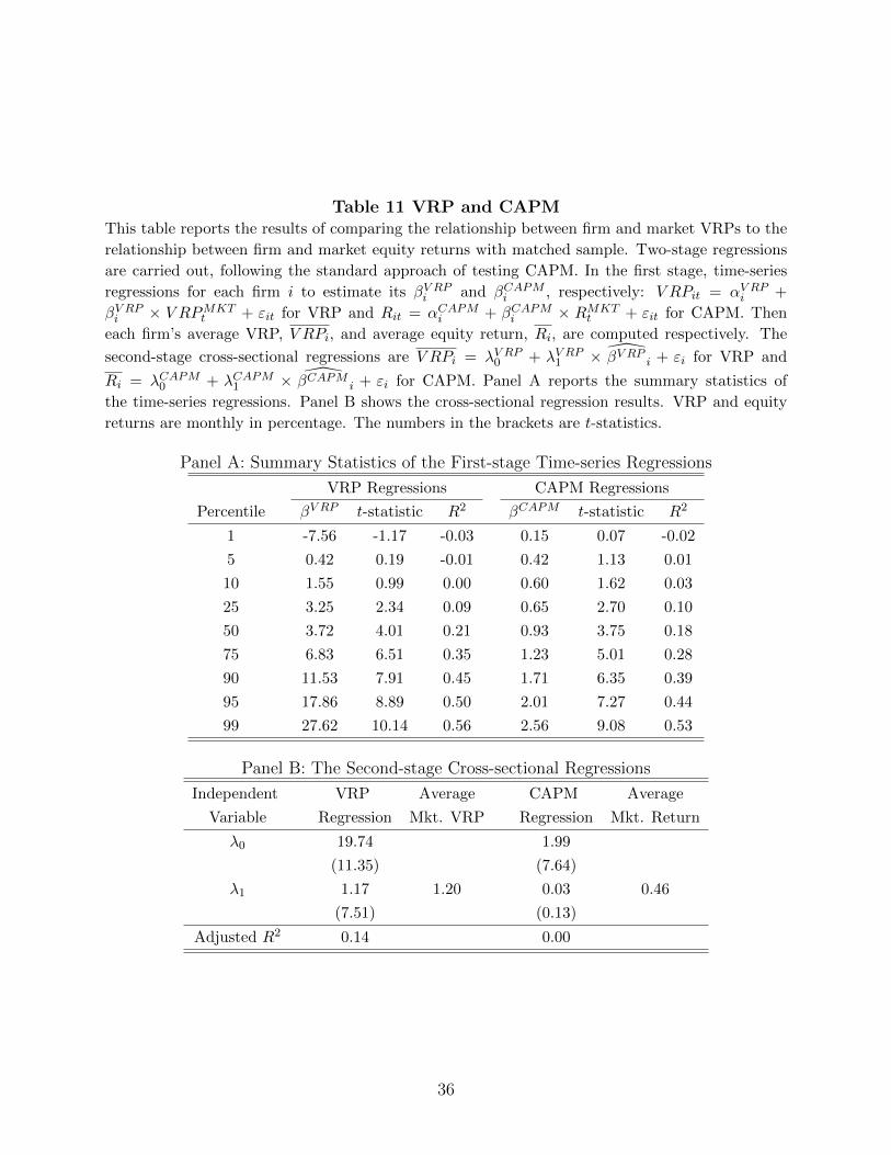
4.4 Cross-Sectional Validation of Market VRP
To examine to what extent firm-level VRP captures the exposure to a systematic variance
risk factor, we compare the relationship between firm and market VRPs to the relationship
between firm and market equity returns with the matched sample. Following the standard
approach of testing CAPM (e.g., Lintner, 1965), we carry out two-stage regressions. In the
first stage, we run time-series regressions for each firm i to estimate its βV RPi and βCAPMi ,
respectively: V RPit = αV RPi + βV RPi × V RPMKT
t + εit
Rit = αCAPMi + βCAPMi ×RMKTt + εit,
(7)
We then compute each firm’s average VRP, V RPi, and average equity return, Ri, respectively.
The second-stage cross-sectional regressions are as following:V RPi = λV RP0 + λV RP1 × β̂V RP i + εi
Ri = λCAPM0 + λCAPM1 × β̂CAPMi + εi.
(8)
The fundamental hypotheses being tested are λV RP0 = 0, λV RP1 = Mean Market VRP;
λCAPM0 = 0, λCAPM1 = Mean Market Return.
Panel A of Table 11 reports the summary statistics of βV RPi and βCAPMi . As indicated
by percentile, the t-statistics of βV RPi are relatively more dispersively distributed and more
significant in the percentiles between 50% and 99%. In addition, the R2s of the VRP regres-
sions are generally higher than their counterparts in the CAPM regressions. The evidence
18
suggests that VRP captures systematic risk more strongly than the well documented equity
returns do. The means of the t-statistics for VRP and equity return regressions are 4.29
and 3.91, respectively. The difference is on average 0.38 with a standard deviation of 0.18.
Unreported mean comparison t-test shows a t-statistic of 2.15, indicating the t-statistic of
the VRP regressions are statistically higher than that of the equity return regressions.
Panel B shows that VRP is significantly related to βV RP with a t-statistic of 7.51, but
equity return is not significantly related to βCAPM . The VRP regression has an adjusted R2
of 14.05 percent, compared to an adjusted R2 of zero for the equity return regression.7 Figure
3 visualizes the fitted VRPs (equity returns) versus the observed VRPs (equity returns). We
find that λV RP1 is 1.17 which is very close to the average market VRP of 1.20, whereas λCAPM1
is 0.03 percent which is much lower than the average monthly market equity return of 0.46
percent. The latter evidence is largely in line with the vast literature on testing CAPM
since Lintner (1965). Although both intercepts λV RP0 and λCAPM0 are rejected to be zeros,
we intentionally have not imposed the risk-free rate restrictions yet, so that we only focus
on whether the slopes are equal to market variance risk premium or market equity return
premium. The above evidence further indicates that firm-level VRPs are able to price the
systematic variance risk factor, much stronger than firm-level equity returns to price the
systematic return risk factor, as advocated in standard asset pricing models.
4.5 A Structural Model with Stochastic Variance Risk
The main finding that variance risk premium (VRP) emerges as a leading explanatory vari-
able for credit spread, suggests that there are two default risk drivers in the underlying firm
asset dynamics. A structural model with stochastic volatility, as in Zhang, Zhou, and Zhu
(2009), can generate the stylized fact that VRP is intimately related to credit spreads, in
addition to the powerful leverage ratio (Collin-Dufresne and Goldstein, 2001).
Assume the same market conditions as in Merton (1974), and one can introduce stochastic
7The adjusted R2 of the VRP regression increases to 0.29 after dropping 14 firms with negative βV RP swithout changing significantly the adjusted R2 of the CAPM regression.
19
variance into the underlying firm-value process:
dAtAt
= (µ− δ)dt+√VtdW1t, (9)
dVt = κ(θ − Vt)dt+ σ√VtdW2t, (10)
where At is the firm value, µ is the instantaneous asset return, and δ is the asset payout
ratio. The asset return variance, Vt, follows a square-root process with long-run mean θ,
mean reversion κ, and volatility-of-volatility parameter σ. Finally, the correlation between
asset return and return volatility is corr (dW1t, dW2t) = ρ.
With proper bankruptcy assumptions, we can solve the equity price, St, as a European
call option on firm asset At with maturity T : St = AtF∗1 − Be−r(T−t)F ∗2 , with r being the
risk-free rate. F ∗1 and F ∗2 are the so-called risk-neutral probabilities. Therefore, the debt
value can be expressed as Dt = At − St, and its price is Pt = Dt/B, where B is the face
value of debt. The credit spread, CSt, is given by:
CSt = − 1
T − tlog(Pt)− r. (11)
The structural credit risk model presented here also implies the following equity variance
process, V st =
(At
St
)2 (∂St
∂At
)2Vt +
(σSt
)2 (∂St
∂Vt
)2Vt + At
S2t
∂St
∂At
∂St
∂VtρσVt . Inside simulation, we can
examine the relationship between credit spread CSt and VRP
V RPt = EQt (RVt+1)− EP
t (RVt+1) (12)
where RVt+1 is the realized variance from five-minute equity returns, and the risk-neutral
expectation EQt (·) and physical expectation EP
t (·) are approximated using the asset volatility
dynamics (10).
Using a calibrated parameter setting for a BBB firm as in Zhang, Zhou, and Zhu (2009),
we simulate 60 month of data of credit spreads, VRP, expected variance, and leverage ratio
for both a Merton (1974) model and a stochastic volatility model (as above). Table 12
report the OLS regressions on explaining credit spreads with those proxies for underlying
risk factors in asset value and volatility dynamics.
20
For the Merton (1974) model, leverage ratio will drive expected variance to be statistically
insignificant, even though variance itself has a significant positive effect on credit spread.
Note that for Merton model, although the asset volatility is constant, the equity volatility
is time-varying; because asset value is time-varying and equity volatility is approximately
leverage adjusted asset volatility. Therefore equity volatility does explain credit spread, but
its effect is mostly subsumed when leverage ratio is included in the regression.
However, for the two factor stochastic volatility model, not only expected variance, VRP,
and leverage ratio all have significant positive effect on credit spreads; but also any two
variables combined together would both remain statistically significant with positive signs.
In particular, the powerful leverage ratio cannot crowd out VRP or expected variance. This
is due to the fact that both asset value and asset volatility are time-varying priced risk
factors, and VRP or expected variance is not redundant to leverage ratio as in the case of
one-factor Merton (1974) model. This result is qualitatively consistent with what we have
discovered here for a large cross-section of individual firms’ CDS spreads and VRPs.
5 Conclusions
Investors demand variance risk premium (VRP) as a compensation for firms’ exposures to a
systematic factor. Such a risk premium may arise from the time-varying fluctuations in the
underlying cash flow or consumption volatility (Bansal and Yaron, 2004; Bollerslev, Tauchen,
and Zhou, 2009). Recent studies suggest that market VRP captures the macroeconomic
uncertainty or systematic variance risk that constitute a critical component in explaining
the aggregate credit spread indices (Zhou, 2009; Buraschi, Trojani, and Vedolin, 2009).
In this paper we carry out a comprehensive investigation on the relationship between the
firm-level VRPs and credit spreads, and justify empirically that VRP provides a risk-based
explanation for the credit spread variations.
We illustrate that VRPs of individual firms, estimated by the difference between model-
free implied and expected variances, possess a significant explanatory power for credit default
swap (CDS) spreads. Importantly, such predictability cannot be substituted for by that
21
of market- and firm-level credit risk factors identified in previous research. In addition,
firm-level VRP dominates the well-documented market-level VRP or VIX in capturing the
macroeconomic uncertainty or systematic variance risk premium embedded in CDS spreads.
The predictive power of VRP increases as the credit quality of CDS entities deteriorates and
as the maturity of CDS contract increases. Leverage ratio and VRP emerge as two leading
predictors of firms’ credit spreads, pointing to asset value and stochastic volatility as two
underlying risk drivers.
Empirical evidence also suggests that the superior explanatory power of VRP for CDS
spreads tends to be stronger over monthly and quarterly horizons, while that of implied
variance over weekly horizon. Also, the aggregate VRP seems to Granger-causes implied
and expected variances, but not vise versa. A principle component analysis indicates that
firms’ VRPs have a much larger systematic component relative to implied and expected
variances. These additional findings imply that firms’ VRP may be a good measure of
exposure to a systemic variance risk or economic uncertainty factor, which is consistent
with the fact that the cross-section of firm’s VRPs can be used to validate the market VRP
correctly. Further more, the stylized predictability pattern of VRP for credit spread can be
reproduced in simulation by a structural model with stochastic variance.
22
References
Andersen, Torben G., Tim Bollerslev, Francis X. Diebold, and Heiko Ebens (2001a), “The
Distribution of Realized Stock Return Volatility,” Journal of Financial Economics , vol. 61,
43–76.
Andersen, Torben G., Tim Bollerslev, Francis X. Diebold, and Paul Labys (2001b), “The
Distribution of Realized Exchange Rate Volatility,” Journal of the American Statistical
Association, vol. 96, 42–55.
Bansal, Ravi and Amir Yaron (2004), “Risks for the Long Run: A Potential Resolution of
Asset Pricing Puzzles,” Journal of Finance, vol. 59, 1481–1509.
Barndorff-Nielsen, Ole and Neil Shephard (2002), “Econometric Analysis of Realised Volatil-
ity and Its Use in Estimating Stochastic Volatility Models,” Journal of Royal Statistical
Society Series B , vol. 64, 253–280.
Berndt, Antj, Aziz A. Lookman, and Iulian Obreja (2006), “Default Risk Premia and Asset
Returns,” Carnegie Mellon University, Working Paper.
Bhamra, Harjoat, Lars-Alexander Kuhn, and Ilya Strebulaev (2009), “The Levered Equity
Risk Premium and Credit Spreads: A United Framework,” Standford University, Working
Paper.
Blanco, Roberto, Simon Brennan, and Ian Marsh (2005), “An Empirical Analysis of the Dy-
namic Relationship Between Investment-Grade Bonds and Credit Default Swaps,” Journal
of Finance, vol. 60, 2255–2281.
Bollerslev, Tim, George Tauchen, and Hao Zhou (2009), “Expected Stock Returns and
Variance Risk Premia,” Review of Financial Studies,” Review of Financial Studies , vol. 22,
4463–4492.
Britten-Jones, Mark and Anthony Neuberger (2000), “Option Prices, Implied Price Processes
and Stochastic Volatility,” Journal of Finance, vol. 55, 839–866.
Buraschi, Andrea, Fabio Trojani, and Andrea Vedolin (2009), “The Joint Behavior of Credit
Spreads, Stock Options and Equity Returns When Investors Disagree,” Imperial College
London Working Paper.
Campbell, John Y. and Glen B. Taksler (2003), “Equity Volatility and Corporate Bond
Yields,” Journal of Finance, vol. 58, 2321–2349.
Cao, Charles, Fan Yu, and Zhaodong Zhong (2008), “How Important Is Option-Implied
Volatility for Pricing Credit Default Swaps,” Forthcoming.
23
Carr, Peter and Liuren Wu (2008a), “Stock Options and Credit Default Swaps: A Joint
Framework for Valuation and Estimation,” New York University, Working Paper.
Carr, Peter and Liuren Wu (2008b), “Variance Risk Premia,” Review of Financial Studies ,
vol. 22, 1311–1341.
Chen, Hui (2009), “Macroeconomic Conditions and the Puzzles of Credit Spreads and Capital
Structure,” Journal of Finance, page forthcoming.
Chen, Long, Pierre Collin-Dufresne, and Robert Goldstein (2009), “On the Relation Between
the Credit Spread Puzzle and the Equity Premium Puzzle,” Review of Financial Studies ,
vol. 22, 3367–3409.
Collin-Dufresne, Pierre and Robert Goldstein (2001), “Do Credit Spreads Reflect Stationary
Leverage Ratios?” Journal of Finance, vol. 56, 1929–1957.
Collin-Dufresne, Pierre, Robert S. Goldstein, and Spencer Martin (2001), “The Determinants
of Credit Spread Changes,” Journal of Finance, vol. 56, 2177–2207.
Cox, John, Stephen Ross, and Mark Rubinstein (1979), “Option Pricing: A simplified ap-
proach,” Journal of Financial Economics , vol. 7, 229–263.
Cremers, Martijn, Joost Driessen, Pascal Maenhout, and David Weinbaum (2008), “Individ-
ual Stock-Option Prices and Credit Spreads,” Journal of Banking and Finance, vol. 32,
2706–2715.
David, Alexander (2008), “Inflation Uncertainty, Asset Valuations, and the Credit Spread
Puzzles,” Reveiew of Financial Studies , vol. 21, 2487–2534.
Drechsler, Itamar and Amir Yaron (2009), “What’s Vol Got to Do With It.” University of
Pennsylvania, Working Paper.
Elton, Edwin, Martin Gruber, Deepak Agrawal, and Christopher Mann (2001), “Explaining
the Rate Spread on Corporate Bonds,” Journal of Finance, vol. 56, 247–277.
Ericsson, Jan, Kris Jacobs, and Rodolfo Oviedo (2004), “The Determinants of Credit Default
Swap Premia,” McGill University, Working Paper.
Ericsson, Jan, Joel Reneby, and Hao Wang (2006), “Can Structural Models Price Default
Risk? Evidence from Bond and Credit Derivative Markets,” McGill University, Working
Paper.
24
Huang, Jing-Zhi and Ming Huang (2003), “How Much of the Corporate-Treasury Yield
Spread is Due to Credit Risk? A New Calibration Approach,” Pennsylvania State Uni-
versity, Working paper.
Jiang, George and Yisong Tian (2005), “The Model-Free Implied Volatility and Its Informa-
tion Content,” Review of Financial Studies , vol. 18, 1305–1342.
Jones, Philip, Scott Mason, and Eric Rosenfeld (1984), “Contingent Claims Analysis of
Corporate Capital Structures: An Empirical Investigation,” Journal of Finance, vol. 39,
611–627.
Lintner, John (1965), “Security Prices, Risk and Maximal Gains from Diversification,” Jour-
nal of Finance, vol. 20, 587–615.
Longstaff, Francis, Sanjay Mithal, and Eric Neis (2005), “Corporate Yield Spreads: Default
Risk or Liquidity? New Evidence from the Credit Default Swap Market,” Journal of
Finance, vol. 60, 2213–2253.
Longstaff, Francis and Eduardo Schwartz (1995), “Valuing Credit Derivatives,” Journal of
Fixed Income, vol. June, 6–12.
Merton, Robert (1974), “On the Pricing of Corporate Debt: The Risk Structure of Interest
Rates,” Journal of Finance, vol. 29, 449–479.
Petersen, Mitchell (2009), “Estimating Standard Errors in Finance Panel Data Sets: Com-
paring Approaches,” Review of Financial Studies , vol. 22, 435–480.
Tang, Dragon Yongjun and Hong Yan (2008), “Liquidity, Liquidity Spillovers, and Credit
Default Swap Spreads,” University of Hong Kong, Working Paper.
Uncertainty,” Federal Reserve Board, Working Paper.
Zhu, Haibin (2006), “An Empirical Comparison of Credit Spreads Between the Bond Market
and the Credit Default Swap Market,” Bank of International Settlements, Working Paper.
25
Tab
le1:
Desc
rip
tive
Sta
tist
ics
-C
DS
Spre
ads,
Vari
ance
Ris
kP
rem
ium
,Im
pli
ed
Vari
ance
and
Exp
ect
ed
Vari
ance
.T
his
tab
lep
rese
nts
the
sum
mar
yst
atis
tics
—av
erag
eac
ross
the
382
firm
s—of
the
five
-yea
rC
DS
spre
ads
and
our
ben
chm
ark
Var
ian
ce
Ris
kP
rem
ium
(VR
P)
mea
sure
(Pan
elA
),m
od
el-f
ree
imp
lied
vari
ance
san
dex
pec
ted
vari
ance
s(P
anel
B).
Th
eC
DS
spre
ads
are
inb
asis
poin
ts.
Th
eV
RP
isco
mp
ute
das
the
spre
adb
etw
een
mod
el-f
ree
imp
lied
vari
ance
and
exp
ecte
dva
rian
ce.
Th
eim
pli
edva
rian
ceis
the
mod
el-f
ree
imp
lied
vari
an
ce.
Th
eex
pec
ted
vari
ance
isth
eli
nea
rfo
reca
stof
real
ized
vari
ance
by
lagg
edim
pli
edan
dre
aliz
edva
rian
ce.
Th
eav
erage
Mood
y’s
and
S&
Pra
tin
gs
of
the
CD
Sre
fere
nce
enti
ties
ran
geb
etw
een
AA
Aan
dC
CC
.T
he
nu
mb
ers
offi
rms
inea
chra
tin
g
cate
gory
are
rep
orte
din
the
seco
nd
colu
mn
inP
anel
A.
AR
(1)
den
otes
auto
corr
elat
ion
wit
hon
ela
g.
Pan
elA
:T
he
mea
ns
ofth
est
atis
tics
ofC
DS
spre
ads
and
VR
Pac
ross
indiv
idual
firm
s
CD
SS
pre
adV
RP
Rat
ing
Fir
mN
um
ber
Mea
nS
DS
kew
.K
urt
.A
R(1
)M
ean
SD
Skew
.K
urt
.A
R(1
)
AA
A7
17.4
312
.04
1.54
5.92
0.88
7.34
9.08
1.59
6.87
0.46
AA
17
20.9
710
.29
0.97
3.62
0.87
10.1
611
.03
2.00
9.01
0.40
A101
33.8
418
.18
1.33
4.98
0.86
16.9
715
.43
1.46
5.86
0.52
BB
B199
77.0
739
.06
1.10
4.41
0.84
23.2
317
.81
1.23
5.25
0.37
BB
133
220.
8085
.26
0.90
4.84
0.74
43.7
125
.87
1.05
4.67
0.35
B65
368.
4411
9.56
0.39
2.98
0.66
63.8
935
.73
0.88
4.08
0.24
CC
C14
603
.10
237.
080.
693.
570.
6082
.03
39.7
80.
162.
940.
31
Tota
l382
151.
1858
.94
1.01
4.44
0.80
32.8
021
.57
1.20
5.20
0.38
Pan
elB
:T
he
mea
ns
ofth
est
atis
tics
ofIV
and
EV
acro
ssin
div
idual
firm
sIm
pli
edV
aria
nce
Exp
ecte
dV
aria
nce
Rati
ng
Mea
nS
DS
kew
.K
urt
.A
R(1
)M
ean
SD
Ske
w.
Ku
rt.
AR
(1)
AA
A40.3
827.
391.
757.
230.
6533
.04
18.7
01.
106.
710.
65
AA
45.
9827
.08
1.72
6.92
0.60
35.8
217
.22
1.62
6.41
0.52
A66
.90
37.4
51.
445.
440.
6649
.93
23.2
11.
435.
320.
58
BB
B88.
1441.
431.
215.
040.
5864
.91
25.5
61.
224.
990.
50
BB
144.
2256
.45
1.13
4.86
0.54
100.
5133
.68
1.12
4.85
0.32
B193
.06
72.3
01.
014.
230.
5112
9.17
41.3
61.
004.
210.
28
CC
C234
.52
69.0
00.
533.
620.
4115
2.49
36.3
30.
503.
620.
31
Tota
l11
2.1
847.
891.
225.
050.
5779
.38
28.8
01.
224.
220.
45
26
Table 2 Summary Statistics - the Market and Firm Characteristic Variables.This table reports the descriptive statistics of the market- and firm-level control variables. For firm
characteristics, we report the averages of the statistics across 382 firms. The market VRP is the
difference between implied variance and expected variance of the S&P 500 index as in Bollerslev,
Tauchen and Zhou (2009). The S&P 500 return, is the proxy for the overall state of the economy.
The one year swap rate is the proxy for the risk-free interest rate. The Moody’s default premium
slope, defined as Baa yield spread minus Aaa yield spread is the default risk premium in the
corporate bond market. The difference of five-year swap rate and five-year Treasury rate is a proxy
for fixed income market illiquidity. The asset turnover is computed as sales divided by total assets.
The price-earnings ratio is the ratio of price over earnings. The market-to-book ratio is the ratio of
market equity to book equity. The return on assets is computed earnings divided by total assets.
Table 6 The CDS Spreads of Different Maturity Terms and VRPThis table reports the regression results of CDS spreads of all maturities on the VRP computed with
model free implied variance IV minus expected variance EV estimated with high frequency equity
returns. We adjust two-dimensional (firm and time) clustered standard errors in the regressions as
in Petersen (2009). The numbers in the brackets are t-statistics.
Asset Turnover Ratio −2.87 −3.61 −1.01 3.10 3.40 4.50
(−0.69) (−0.74) (−0.20) (0.59) (0.63) (0.84)
Price-earnings Ratio −0.00 −0.00 −0.01 −0.01 −0.01 −0.00
(−0.14) (−0.27) (−0.67) (−1.05) (−0.99) (−0.66)
Market/Book Ratio −0.01 −0.01 −0.01 −0.02 −0.02 −0.03
(−1.42) (−2.62) (−2.26) (2.79) (−3.30) (−3.38)
Return on Assets −7.75 −15.25 −16.24 −23.56 −30.56 −33.55
(−0.35) (−0.57) (−0.61) (−0.92) (−1.22) (−1.37)
Log Sales −2.59 −3.33 −6.51 −12.23 −12.68 −14.59
(−0.76) (−0.88) (−1.63) (−3.06) (−3.13) (−3.64)
Constant −1.92 −18.96 −14.66 −0.31 −6.59 6.38
(−0.07) (−0.66) (−0.48) (−0.01) (−0.21) (0.20)
Adjusted R2 0.40 0.41 0.46 0.49 0.50 0.51
31
Table 7 CDS Spreads and VRPs of Different Implied VariancesThis table reports the regression results of CDS spreads on VRPs computed from different measures
of implied variances. Besides the benchmark VRP computed from model-free implied variance, we
use VRP constructed from implied variances of out-of-the-money (OTM), at-the-money (ATM) and
in-the-money (ITM) put options, together with those of out-of-the-money (OTM), at-the-money
(ATM) and in-the-money (ITM) call options. We adjust two-dimensional (firm and time) clustered
standard errors in the regressions as in Petersen (2009). The numbers in the brackets are t-statistics.
Table 8 VRP Versus Implied Variance and Expected Variance.This table compares the predictability of VRP on CDS spreads to that of model-free implied and
expected variances for 5-year maturity CDS spreads. Regression (1) to (3) report the multivariate
regression results for VRP, implied and expected variances, along with all control variables. Re-
gression (4) to (6) report the regression results of CDS spreads on each pairs of VRP, implied and
expected variances respectively, along with all control variables. We adjust two-dimensional (firm
and time) clustered standard errors in the regressions as in Petersen (2009). The numbers in the
Asset Turnover Ratio 3.09 −2.99 −3.39 −2.19 −2.19 −2.19
(0.59) (−0.54) (−0.56) (−0.40) (−0.40) (−0.40)
Price-earnings Ratio −0.01 −0.00 −0.01 −0.00 −0.00 −0.00
(−1.05) (−0.58) (−0.66) (−0.63) (−0.63) (−0.63)
Market/Book Ratio −0.02 −0.01 −0.01 −0.02 −0.02 −0.02
(−2.79) (−2.49) (−2.22) (−2.56) (−2.56) (−2.56)
Return on Assets −23.56 −22.78 −45.42 −19.65 −19.65 −19.65
(−0.92) (−0.89) (−1.73) (−0.77) (−0.77) (−0.77)
Log Sales −12.23 −7.27 −9.30 −7.58 −7.58 −7.58
(−3.06) (−1.72) (−2.12) (−1.82) (−1.82) (−1.82)
Constant −0.31 −26.87 −13.34 −25.59 −25.59 −25.59
(−0.01) (−0.83) (−0.40) (−0.80) (−0.80) (−0.80)
Adjusted R2 0.49 0.52 0.48 0.52 0.52 0.52
33
Table 9 Different Data Frequency Analysis and Granger CausalityThis table reports the results of different data frequency analysis and Granger Causality tests.
Panel A shows the regression results of CDS on VRP, in the absence/presence of IV for weekly,
monthly and quarterly data frequency. Panel B reports the Granger Causality tests result. We use
three lags in the regressions as R2 stops increasing significantly at three lags. The numbers in the
brackets are t-statistics.
Panel A: Data Frequency Analysis
Frequency
Independent Variable Weekly Monthly Quarterly
VRP 1.39 -0.24 2.78 0.06 2.57 0.68
(6.44) (-1.43) (10.03) (2.41) (10.14) (3.00)
IV 0.10 1.08 0.95
(10.71) (7.46) (6.41)
Constant 70.49 0.24 28.00 -13.20 29.71 -7.14
(9.24) (0.03) (5.89) (-1.63) (6.83) (-0.95)
Adjusted R2 0.14 0.26 0.34 0.39 0.35 0.40
Panel B: Granger Causality Analysis
Dependent Independent
Variable Variable R2
Cont V RP t−1 V RP t−2 V RP t−3 IV t−1 IV t−2 IV t−3
Table 10 Principal Component Analyses of CDS Spreads, VRP, IV and EVThis table reports the principal component analysis of CDS spreads, VRP, implied and expected
variances. We select firms with 48 monthly observations starting in January 2004. The sample
contains 194 firms. VRP is explained mostly by first three components (91.62% cumulatively),
whereas IV and EV are driven marginally by several components. Robustness checks with various
samples show that sample selection does not change the results qualitatively. E: Explained. C:
Cumulative.
CDS Spreads VRP IV EV
Component E. % C. % E. % C. % E. % C. % E. % C. %
1 60.36 60.36 77.93 77.93 53.67 53.67 64.03 64.03
2 13.44 73.80 9.97 87.90 10.79 64.47 11.78 75.81
3 6.10 79.90 3.72 91.62 5.58 70.05 4.45 80.26
4 4.21 84.11 2.20 93.82 3.55 73.60 2.66 82.92
5 3.42 87.52 1.76 95.58 3.22 76.82 2.36 85.28
6 2.93 90.45 0.78 96.37 2.25 79.07 1.50 86.78
7 1.74 92.20 0.73 97.10 1.96 81.03 1.27 88.05
8 1.35 93.54 0.48 97.57 1.76 82.79 1.09 89.14
9 1.17 94.72 0.38 97.95 1.65 84.45 0.93 90.07
10 1.16 95.88 0.30 98.25 1.46 85.90 0.88 90.95
35
Table 11 VRP and CAPMThis table reports the results of comparing the relationship between firm and market VRPs to the
relationship between firm and market equity returns with matched sample. Two-stage regressions
are carried out, following the standard approach of testing CAPM. In the first stage, time-series
regressions for each firm i to estimate its βV RPi and βCAPMi , respectively: V RPit = αV RPi +
βV RPi × V RPMKTt + εit for VRP and Rit = αCAPMi + βCAPMi × RMKT
t + εit for CAPM. Then
each firm’s average VRP, V RPi, and average equity return, Ri, are computed respectively. The
second-stage cross-sectional regressions are V RPi = λV RP0 + λV RP1 × β̂V RP i + εi for VRP and
Ri = λCAPM0 + λCAPM1 × β̂CAPMi + εi for CAPM. Panel A reports the summary statistics of
the time-series regressions. Panel B shows the cross-sectional regression results. VRP and equity
returns are monthly in percentage. The numbers in the brackets are t-statistics.
Panel A: Summary Statistics of the First-stage Time-series Regressions
VRP Regressions CAPM Regressions
Percentile βV RP t-statistic R2 βCAPM t-statistic R2
1 -7.56 -1.17 -0.03 0.15 0.07 -0.02
5 0.42 0.19 -0.01 0.42 1.13 0.01
10 1.55 0.99 0.00 0.60 1.62 0.03
25 3.25 2.34 0.09 0.65 2.70 0.10
50 3.72 4.01 0.21 0.93 3.75 0.18
75 6.83 6.51 0.35 1.23 5.01 0.28
90 11.53 7.91 0.45 1.71 6.35 0.39
95 17.86 8.89 0.50 2.01 7.27 0.44
99 27.62 10.14 0.56 2.56 9.08 0.53
Panel B: The Second-stage Cross-sectional Regressions
Table 12 Simulated Relationship between CDS Spread and VRPThis table reports the OLS regression result using simulated ten years of monthly data from a
Merton (1974) model and a stochastic volatility model (Zhang, Zhou, and Zhu, 2009) for a rep-
resentative BBB rating firm. The dependent variable is five-year credit spread, and explanatory
variables are expected variance (EV) estimated by annual historical variance, variance risk pre-
mium (VRP) estimated based on monthly realized variance, and market leverage ratio (LEV) only
observable inside the simulation. Numbers in parentheses are t-statistics.
Independent Merton Model Stochastic Volatility Model