Finance and Economics Discussion Series Divisions of Research & Statistics and Monetary Affairs Federal Reserve Board, Washington, D.C. Auto Sales and Credit Supply Kathleen W. Johnson, Karen M. Pence, and Daniel J. Vine 2014-82 NOTE: Staff working papers in the Finance and Economics Discussion Series (FEDS) are preliminary materials circulated to stimulate discussion and critical comment. The analysis and conclusions set forth are those of the authors and do not indicate concurrence by other members of the research staff or the Board of Governors. References in publications to the Finance and Economics Discussion Series (other than acknowledgement) should be cleared with the author(s) to protect the tentative character of these papers.
Transcript
Finance and Economics Discussion SeriesDivisions of Research & Statistics and Monetary Affairs
Federal Reserve Board, Washington, D.C.
Auto Sales and Credit Supply
Kathleen W. Johnson, Karen M. Pence, and Daniel J. Vine
2014-82
NOTE: Staff working papers in the Finance and Economics Discussion Series (FEDS) are preliminarymaterials circulated to stimulate discussion and critical comment. The analysis and conclusions set forthare those of the authors and do not indicate concurrence by other members of the research staff or theBoard of Governors. References in publications to the Finance and Economics Discussion Series (other thanacknowledgement) should be cleared with the author(s) to protect the tentative character of these papers.
Auto Sales and Credit Supply
Kathleen Johnson, Karen Pence, and Daniel Vine
Board of Governors of the Federal Reserve System
September 2014
Abstract. Vehicle purchases fell by more than 20 percent during the 2007-09 recession, and auto loan originations fell by a third. We show that vehicle purchases typically account for an outsized share of the contraction in economic activity during a recession, in part because a concurrent tightening in auto lending conditions makes car purchases less affordable for many households. We explore the link between lending conditions and vehicle purchases with a novel gauge of credit supply conditions—household perceptions of vehicle financing conditions as measured on the Reuters/University of Michigan Survey of Consumers. In both a vector auto-regression estimated on aggregate data and a logit regression estimated on household-level data, this measure indicates that credit conditions are a significant influence on auto sales, as large as factors such as unemployment and income. Estimates from the household-level model show that the new car purchases of households that are more likely to depend on credit are particularly sensitive to assessments of financing conditions, and that households are a bit more likely to purchase vehicles when they expect interest rates to rise in the next year. The results contribute to the literature validating the usefulness of survey measures of household perceptions for forecasting macroeconomic activity.
Author contact information: [email protected], [email protected], [email protected]. We thank Samuel Ackerman, Angus Chen, Andrew Loucky, Brett McCully, Meredith Richman, Mark Wicks, and Jessica Zehel for terrific research assistance. We thank our Federal Reserve colleagues, Moshe Buchinsky, and seminar participants at the NBER Summer Institute, the OCC and the Homer Hoyt Institute for helpful insights and conversations. We are grateful to Bob Hunt, Avi Peled, Sharon Tang, and Chellappan Ramasamy at the Philadelphia Fed for generously providing us with estimates from credit bureau data. The views in this paper are the authors’ alone and do not necessarily reflect the views of the Board of Governors of the Federal Reserve System or its staff.
1
1. Introduction
Real consumer purchases of new and used motor vehicles and the flow of consumer
credit used to purchase them contracted considerably during the 2007-09 recession.1 Real
consumer purchases of motor vehicles dropped 22 percent between the end of 2007 and the first
quarter of 2009, and loan originations for motor vehicles fell 33 percent. Factors that likely
contributed to the drop in sales included the sharp rise in the unemployment rate, the plunge in
household wealth, a spate of bankruptcies in the motor vehicle industry that depressed the value
of trade-in vehicles for some brands, and the steep run-up in gasoline prices in the summer of
2008. In addition, the financial crisis constrained the ability of finance companies, banks, and
even credit unions to originate auto loans. Auto lending conditions appeared to tighten
considerably during this period, with average interest rate spreads on new car loans rising from
about 2¼ percentage points in mid-2007 to more than 4¾ percentage points in the first quarter of
2009.
Although the decreases in consumer purchases of motor vehicles and consumer auto
loans during the 2007-09 recession were quite large, these contractions are not unusual. Declines
in purchases of motor vehicles typically account for almost two-thirds of the slowdown in
growth of real durable goods consumption during recessions, even though vehicles represent
only about a third of durable goods purchases. Part of this decline seems to stem from the fact
that consumers may delay vehicle purchases when they are uncertain about their economic
prospects, and part of the decline likely reflects the fact that the supply of credit often tightens
during recessions and may reduce the affordability of a car purchase. This relationship between
credit supply and vehicle purchases is the focus of our paper.
Identifying the effects of changes in credit conditions on real activity is a classic topic in
macroeconomics. The traditional life-cycle framework suggests that in the absence of borrowing
constraints, interest rates should be the only loan contract term that affects vehicle demand (see
Chah, Ramey, and Starr, 1995, for one example). However, the vehicle demand of borrowing-
constrained households depends on other contract terms besides the interest rate, such as the loan
amount, the required down payment, and the loan maturity. Data on motor vehicle loan contracts
1 Motor vehicles in this paper are defined as passenger cars and light trucks, which include vans, pickups, sports-utility and cross-utility vehicles. We use the terms “autos” and “cars” interchangeably with “motor vehicles.”
2
suggest that many vehicle purchasers are borrowing constrained (Attanasio, Goldberg, and
Kyriazidou, 2008). The sensitivity of vehicle purchases to changes in transitory income has also
been presented as evidence of borrowing constraints, as shown in the context of tax refunds
Souleles, Johnson, and McClelland, 2013); an increase in the minimum wage (Aaronson,
Agarwal, and French, 2012); an increase in Social Security benefits (Wilcox, 1989); and
expansions of health insurance (Leininger, Levy, and Schanzenbach, 2010). These papers
suggest that this excess sensitivity may be concentrated among purchases of new cars by lower-
income households that are presumably more likely to depend on credit to purchase vehicles.
Similarly, Mian, Rao, and Sufi (2013) and Mian and Sufi (2014) show that the marginal
propensity to purchase vehicles from changes in housing wealth—which appear to affect
household borrowing constraints—is largest in zip codes with lower average income and higher
ratios of mortgage debt to house values.
In this paper, we explore the role that auto lending conditions play in consumer purchases
of motor vehicles. We first document the significant swings in auto sales, auto loans, and credit
availability that typically occur over the business cycle, including the recent 2007-09 recession.
We then look for evidence of a causal link between credit supply and auto purchases. Two
issues make this exercise challenging. First, it is difficult, if not impossible, to observe the credit
supply conditions that apply to each consumer, as loan contract terms are observed only for
households who purchase cars. Second, observed interest rates and other loan terms are partly
endogenous, reflecting changes in the average credit quality of households and overall demand
conditions. For example, the interest rates for new cars are often subsidized by the
manufacturers’ affiliated finance companies (“captive” financing companies). These subsidies,
which are known as interest subvention, typically occur when vehicle sales are soft.
In our empirical work, we use household perceptions of financing conditions, as
measured on the Reuters/University of Michigan Surveys of Consumers (herein, “Michigan
survey”) to explore the relationship between lending conditions and vehicle sales. These
perceptions questions are asked of all households, including those who do not purchase vehicles.
We assume that the household responses primarily reflect credit supply conditions, and, indeed,
we show that these responses vary in sensible ways with other indicators of credit supply. To the
3
best of our knowledge, the relationship between these subjective assessments of financing
conditions and vehicle purchases has not been explored previously, and doing so is one of the
contributions of this paper.
We estimate the relationship between financing conditions and vehicle sales both with a
vector auto-regression (VAR) based on aggregate data and with logit regressions based on
previously unexplored household-level data from the Michigan survey. In the VAR, the effects
of credit conditions on motor vehicle purchases are measured with the response of purchases to
shocks identified recursively with variable ordering. In the logit regressions, we measure the
effect of a household’s assessment of auto finance conditions on the probability it buys a car,
holding constant the detailed information we observe on the economic circumstances of each
household. We measure these household assessments well in advance of the vehicle-purchase
decision, and therefore avoid simultaneity bias.
The two models use different identification assumptions, estimation techniques, and
source data, and yet both models suggest a relatively strong and causal relationship between
credit supply and vehicle purchases. In both models, the effects of financing conditions on sales
are as large, if not larger, than traditional determinants of vehicle purchases such as income and
unemployment. The household-level model suggests that perceived financing conditions are
particularly important for purchases of new cars by households who may be more likely to
depend on credit for their purchases, such as those who do not own stock or have a college
degree. This result is consistent with the studies referenced earlier that find excess sensitivity of
new auto purchases to increases in income among lower-income households. The household-
level model also suggests that consumers are a bit more likely to purchase cars when they
anticipate that interest rates will rise in the next year. Overall, the relationships that we find
between households’ perceptions of vehicle finance conditions and their subsequent car
purchases are consistent with other studies that show that measures of consumer perceptions and
expectations can be useful in forecasting economic outcomes.2
In summary, we find that changes in credit conditions over the business cycle
significantly affect vehicle sales. In the 2007-09 recession, as in previous recessions, credit
2 For recent examples, see French, Kelley, and Qi (2013) and van der Klauuw (2012).
4
conditions tightened, and loan originations and vehicle sales fell. We show that the changes in
vehicle purchases and vehicle loans did not look particularly unusual over this period despite the
severity of the 2008 financial crisis. That said, some of the mechanisms by which credit
tightened were different from previous business cycles, as the sources of funding for auto loans
appear to have shifted over time. For example, the asset-backed commercial paper and asset-
backed securities market came under significant strain during the financial crisis, and the shocks
to these sectors appear to have affected motor vehicle sales (Ramcharan, van den Heuvel, and
Verani, forthcoming; Benmelech, Meisenzahl, and Ramcharan, 2014).3
2. Motor Vehicle Spending and the Business Cycle
Real (inflation-adjusted) personal consumption expenditures (PCE) for motor vehicles—
which includes both new and used vehicles—fell 22 percent during the 2007-09 recession, as
shown in figure 1. The decline was the largest in several decades, but the declines in motor
vehicle spending during recessions tend to be large; real spending on motor vehicles fell 28
percent during the 1969-70 recession and by 14 percent in the 1980 and 1990-91 recessions.
The other components of PCE shown in figure 1, which exclude purchases of motor
vehicles, also fell during the 2007-09 recession.4 In order to put the 2007-09 recession into
historical context and to compare vehicle purchases with purchases of other durable goods,
figure 2 plots the 6-quarter changes of real PCE for motor vehicles and real PCE for other
durable goods. We chose six quarters to match the duration of the 2007-2009 recession. By this
measure, the decline in real PCE for motor vehicles during the 2007-09 recession was large, but
it was not as large as the declines observed during the 1970, 1974-75, and 1980 recessions. In
contrast, the decline in real PCE for other durable goods during the 2007-09 recession was the
most severe decline on record for any 6-quarter period back to at least 1967.
Table 1 presents more formally the contribution of motor vehicles to the business cycle
patterns in PCE for durable goods. Each numbered row of the table shows data for one U.S.
business cycle episode, identified by the NBER dates of the peak and trough, and the memo line
3 See Covitz, Liang, and Suarez (2013) for a discussion of the asset-based commercial paper market during the crisis, and Campbell, Covitz, Nelson, and Pence (2011) for a discussion of the asset-backed securities market. 4 Computers and information processing equipment are excluded from Figure 1 because real spending in these categories has risen so much faster since 1967 than has spending for other durable goods; it is also not particularly cyclical.
5
at the bottom of the table shows the average for the business cycles before the 2007-09 recession.
In an average expansion, real PCE for durable goods grows 5.5 percent at an annual rate from
peak to peak, and during an average recession, it falls 3.1 percent. The contribution of motor
vehicles to the average change in growth from expansions to recessions, shown in the fourth
column of the table, is -5.2 percentage points, or about 60 percent of the average overall change.5
This contribution is about twice as large as the average share of vehicle purchases in overall
durable goods consumption.
During the 2007-09 recession, real PCE for durable goods fell 9 percent at an annual rate
after having risen 6 percent from 2001 to 2007 (row 7). The change in growth, at -15.1
percentage points, was about twice as large as the average decline observed during previous
recessions. The contribution of motor vehicles to this change, at -4.8 percentage points, was
about in line with previous recessions.
3. The relationship between auto purchases and auto loans
About 70 percent of household purchases of new vehicles and 35 percent of household
purchases of used vehicles are financed with auto loans.6 Total auto loan originations for new
and used cars fell from about 29.4 million before the onset of the 2007-09 recession to
19.8 million at the trough, a decline of about 33 percent (figure 3).7 This decline somewhat
exceeded the 22 percent drop in real consumer spending on new and used vehicles over the same
period.
The decline in auto loan originations during the recession was concentrated among
borrowers with lower credit scores (figure 4). Loans originated to borrowers with credit scores
below 620—the traditional cutoff for a subprime credit rating—fell by 54 percent between the
5 The averages in the bottom row of table 1 include observations from the 1981-1982 and 2001 recessions, when—in contrast to the general pattern—purchases of durable goods and motor vehicles increased, and the changes in growth from expansion to recession were also positive. Real PCE for motor vehicles grew at a tepid pace during the 1981-1982 recession and had declined during the brief expansion following the 1980 recession. Motor vehicle spending surged temporarily during the last quarter of the 2001 recession, when the Detroit automakers offered zero-percent financing in effort to boost sales after the September 11 attacks. Another auto industry development that affects the table 1 calculations is the company-wide strike at GM in 1970, which held down auto sales at the end of that year and likely exaggerated the decline in vehicle spending during the 1969-1970 recession. 6 Staff calculation from data on the 2004, 2007, and 2010 Surveys of Consumer Finances. 7 Calculated by staff at the Philadelphia Fed using anonymized credit bureau trade line data provided by Equifax. Units are measured at annual rate.
6
fourth quarter of 2007 and the second quarter of 2009, whereas loan originations to borrowers
with credit scores greater than 780—traditionally considered “superprime” —were little
changed. Subprime loan originations made up about 30 percent of all loan originations in 2006,
so the contraction in this category had a significant effect on overall originations.
Because data on auto loan originations are available back to only the early 2000s, we
cannot use these data to characterize the typical movements of auto loans and auto sales over the
business cycle. However, data on auto loan balances, which are somewhat more difficult to
compare with auto purchases but have a much longer history, suggest that auto loans are a bit
more volatile than sales over the business cycle, although in general the two series move
together.8
To see this, figure 5 shows the 4-quarter changes in vehicle loan balances (solid line)
alongside the 4-quarter changes in the estimated collateral value of recently purchased vehicles
(the dashed line).
The collateral value of recently purchased vehicles plotted in the figure is constructed as
the discounted sum of nominal consumer vehicle purchases made during the past three years or
so. The quarterly discount rate used in the calculation, which we estimate by comparing loan
originations to the changes in loan balances from 2001 to 2007, captures the average pace at
which outstanding loan balances are either paid off by borrowers or written off by lenders. We
estimate this rate to be about 13 percent per quarter, which implies that loan balances should rise
and fall in tandem with the discounted sum of auto purchases made during the past three years if
the share of autos purchased with a loan is constant.9
The peaks and troughs of the two lines in figure 5 are generally well aligned, suggesting
that our estimate of the collateral value of recently purchased vehicles is reasonable and based on
assumptions that do not appear to have changed much over time. The figure also suggests that
8 Auto loan balances totaled $878 billion in the fourth quarter of 2013, accounting for almost 30 percent of total consumer credit outstanding. Total consumer credit outstanding includes most credit extended to individuals excluding loans secured by real estate. Auto loan balances do not include vehicle leases. 9 To estimate the discount rate, we subtract originations in quarter t from loan balances at the end of quarter t. We regress this measure on loan balances at the end of quarter t-1, after first-differencing the data. The coefficient on the lagged loan balances is 0.87 and is significant at the 95% level. The estimate implies that 40 percent of open loan balances reflect loans originated within the past 1 year, 67 percent from the past 2 years, and 82 percent from the past 3 years.
7
loan balances usually grow somewhat more rapidly than purchases during expansions, an
observation that may reflect the cyclical increase during expansions of vehicle purchases by
households that are more reliant on financing. Further, the decline in the growth rate of auto
loan balances between expansions and recessions is somewhat larger than the decline in the
growth rate of consumer vehicle purchases.
Changes in the cost and availability of auto loans during the business cycle
Many consumers use a loan to buy a car, and so changes in auto loan originations during
the business cycle to a large extent just reflect the rise and fall of car purchases. However,
changes in vehicle financing conditions also affect the affordability of a vehicle purchase and
therefore vehicle sales. This effect is pro-cyclical, as lending conditions tend to loosen during
expansions and tighten during recessions. In this regard, also, the 2007-09 recession was not too
different from previous recessions: the deterioration in several measures of auto lending
conditions was large but similar magnitudes of deterioration had been observed in previous
recessions.
We show three measures to demonstrate the cyclicality of lending conditions. First, the
spread between the rate charged on new auto loans and the funding benchmark for lenders—the
two-year swap rate—generally widens in recessions (figure 6). This relationship holds for all the
major suppliers of auto loans—commercial banks, credit unions, and finance companies—as
well as for loans originated at dealerships, which could be financed by any of these types of
institutions. The widening in spreads during the 2007-09 recession appears to be about in line
with previous business cycles.
Second, the willingness of banks to make consumer installment loans, as measured by the
Senior Loan Officer Opinion Survey, also declines in recessions (figure 7). Auto loans are the
largest component of consumer installment loans. The decline observed in this measure during
the 2007-09 recession was matched only by the drop during the 1980 recession.
Third, respondents to the Michigan Survey are asked whether it is a good or bad time to
buy a car, and if so, why. The answers to these questions will feature prominently in our
empirical work. The index of respondents’ assessments of auto credit conditions, defined as the
share who cite low interest rates or easy credit conditions as a reason that it is a good time to buy
8
a car less the share that cite high interest rates or tight credit conditions as a reason it is a bad
time to buy a car, also moves with the business cycle (figure 8). The index is also affected at
times by the much-publicized reduced-rate financing deals offered by the captive finance
companies, such as in the mid-1980s and early 2000s. During the 2007-09 recession, this index
fell to its lowest level since the 1981-82 recession.
4. The Role of Financing Conditions in Motor Vehicle Consumption
We now turn from describing patterns in auto sales and auto lending over the business
cycle to estimating the statistical relationship between these patterns. One way to assess the
causal relationship between lending conditions and vehicle purchases is to include measures of
financing conditions along with the motor vehicle component of PCE and macro variables in a
vector autoregression, as is shown in equation (1).
(1) 1( )t t tY C A L Y U
C is a vector of constants, and the vector Y consists of real PCE for motor vehicles and
five other variables: the real 2-year swap rate; the spread between the interest rate offered by the
captive finance companies and the rate offered by banks—a proxy for interest subvention; an
index constructed from consumer assessments of auto credit conditions in the Michigan survey;
the unemployment rate; and real disposable personal income.10 A(L) is a matrix of polynomials
in the lag operator L. The real variables in Yt are in log differences, and the interest rates and
index variables are in differences. The index of consumer assessments of auto credit conditions
is the Michigan Survey measure shown in figure 8. We also include in the model three lags of
each variable, and Ut is a vector of error terms.11 The model is estimated on quarterly data from
1978:Q3 through 2007:Q4 to ensure that the estimated effects of financing conditions on real
auto purchases are not unduly influenced by the outsized moves in some of the variables during
the 2007-09 recession. As a robustness exercise, we estimate the model with data through 2013;
10 Real PCE for motor vehicles and real disposable personal income are from the National Income and Product Accounts; the 2-year swap rate is from Reuters limited; the unemployment rate is from the Bureau of Labor Statistics; and the rates offered on auto loans from banks and captive finance companies are from the G.19 and G.20 statistical releases from the Federal Reserve. The real rate of interest is calculated as the nominal rate of interest less the 12-month change in the PCE price index. 11 We experimented with several other variables that we ultimately excluded from the model because they were not statistically significant: the aggregate LTV; the log of changes in real household wealth; gasoline prices; headline measures of consumer confidence; and forward-looking survey measures of expected unemployment.
9
except where noted, our results are unchanged when we estimate the regression for this longer
time period.
Figure 9 plots the response of real PCE for motor vehicles to a one standard deviation
shock to each equation. These shocks are identified recursively in the VAR with a standard
Cholesky decomposition. We assume that motor vehicle consumption responds to shocks to real
income and interest subvention in the same quarter and to changes in the unemployment rate, the
real two-year swap rate, and auto credit sentiment with a one-quarter lag.12
The solid line in each panel of figure 9 shows the response of the level of motor vehicle
consumption to a one standard deviation shock to the listed explanatory variable, and the dashed
lines define the 95 percent confidence interval around each point on the solid line. As shown in
the top left panel, a one standard deviation increase to the growth rate of real DPI boosts motor
vehicle consumption by about 1¾ percent after 4 quarters, a magnitude that is statistically
different from zero. Shocks to interest subvention, shown in the top-right panel, boost motor
vehicle consumption by about 1½ percent. The effect of an unemployment rate shock, shown in
the middle-left, is not different from zero. A one standard deviation shock to the 2-year swap
rate reduces motor vehicle consumption by about 2¼ percentage points after 4 quarters.13 A one
standard-deviation increase in consumer sentiment toward car-buying credit conditions,
conditional on all of the other shocks, boosts motor vehicle consumption by 2 percent after about
4 quarters, a magnitude that is statistically different from zero.
We also estimated the VAR separately for new-car and used-car purchases. The results
indicate that financing discounts affect new-car purchases but not used-car purchases; real
interest rates likewise appear to have a larger effect on new-car purchases than on used-car
purchases. The financing-discount result is reassuring, as these promotions are offered almost
12 The variable ordering is similar to the recursive ordering used by Sims (1986) and assumes that real variables respond to the real 2-year swap rate with a lag. The ordering of the variables also implies that consumer sentiment toward car-buying credit conditions responds to the real swap rate shocks in the same period; as a result, shocks to credit sentiment are conditional on underlying interest rates and the value of interest subvention. Moving the unemployment rate ahead of vehicle purchases in the ordering did not much alter the results. 13 The response of vehicle purchases to changes in the real swap rate becomes insignificant (just barely) at most horizons if the end of the sample period is extended from 2007:Q4 to 2013:Q4. If we exclude the years before 1985, when high inflation was a central concern and interest rates were volatile, the response of purchases to the real swap rate decreases, although the response of purchases to financing discounts increases and the response to credit sentiment remains significant and becomes larger than the response of purchases to real income.
10
exclusively for new-car purchases. In contrast, auto credit sentiment has about the same effect
on both new-car and used-car purchases, although the response is more precisely estimated for
used-car purchases.
The impulse responses from the main VAR suggest that consumer assessments of auto
credit conditions play a large role in vehicle purchases even after controlling for underlying
interest rates and interest subvention. To explore what these assessments capture, Table 2
presents the forecast error variance decomposition for this variable in the VAR. The exercise
shows that the perceptions variable moves in a sensible way with interest rate conditions: about a
quarter of the variance of consumer assessments of auto credit conditions after 4 quarters reflects
shocks to the real interest rate and interest subvention. However, slightly more than half of the
variance of car-buying credit sentiment is unexplained by the other variables in the system, as
shown in the last column of the table.
These unexplained changes in the credit assessment index could reflect aspects of lending
conditions not well-captured by the average interest rate; differences between consumer
perceptions of lending conditions and actual lending conditions; or idiosyncratic factors that
affect a household’s ability to access credit at affordable terms. To assess whether the shocks to
consumer credit sentiment partly reflect changes in other (non-interest rate) terms or standards of
credit, we regress the orthogonalized residuals from the consumer assessments of auto credit
conditions equation on the current and lagged values of the Senior Loan Officer Opinion Survey
on Bank Lending Practices (SLOOS) index of the net increase in the willingness of banks to
extend consumer credit.14 The regression is shown in equation 2.
(2) ** **1 2 3
(.002) (.001) (.002) (.002) (.001)0 .005 .001 0 .003t t t t t tu sloos sloos sloos sloos
The sum of the coefficients on the SLOOS index terms is greater than zero, indicating an
increasing willingness to lend boosts the consumer sentiment index, and are statistically
significant as a group.15 The R2 from the regression indicates that about 12 percent of the
14 Information on the SLOOS is available at http://www.federalreserve.gov/boarddocs/SnLoanSurvey/. 15 ** indicates statistical significance at the 5% level. An F test rejects the hypothesis that the coefficients on the SLOOS and its lags are zero; the F statistic is 4.1 with a p-value of .004.
11
variance of the shocks to consumer sentiment toward car-buying credit conditions may reflect
restrictions in credit supply as measured by the SLOOS index.
The results presented here suggest that both actual interest rates, including the amount by
which finance companies subsidize interest rates, and consumer assessments of financing
conditions have an impact on real PCE for motor vehicles, even conditional on other
macroeconomic variables that typically determine consumer spending. In addition, the response
of vehicle purchases to changes in financing conditions is as large, or perhaps even larger, than
its response to traditional macro factors, such as personal income.
5. The effects of financing conditions on household auto purchases
We next explore the relationship between vehicle purchases and financing conditions
with household-level data, which have two key advantages relative to the macro data. First, by
exploiting variation across households, we can control more thoroughly for factors such as
employment and wealth that might be correlated with interest rates. Second, we can identify the
types of households whose auto purchases are more likely to be sensitive to interest rates or other
terms of the loan contract, and thereby gain more insight into the mechanisms underlying the
macroeconomic relationship.
Our household-level analysis is based on microdata from the Michigan survey, in which
about 500 households are asked each month about their expectations for the economy; their
assessment of current conditions; and their income, wealth, and assorted demographic
characteristics. Among these variables, as noted earlier, is the household’s assessment of
vehicle-purchasing conditions. Households are interviewed twice for the survey, with the two
interviews separated by six months. We supplement these data with a special module on vehicle
purchases that the Federal Reserve has sponsored on the survey about three times per year since
2003. These data include an indicator for whether the household purchased a new or used car
during the past six months.
We use these data to estimate logit regressions that relate a household’s decision to
purchase a vehicle to its beliefs about vehicle financing conditions and its personal financial
situation. Our estimation takes advantage of the short-panel aspect of the survey. The dependent
variable is an indicator of whether the household reported in the second interview that it had
12
purchased an automobile in the previous six months. The independent variables are measured at
the time of the first interview and include measures of financing conditions and a host of
macroeconomic and demographic controls. By using responses from the first interview as the
independent variables, we reduce the simultaneity problems that complicate identification of
demand functions.
Our analysis focuses on two measures of financing conditions from the Michigan survey.
First, survey respondents are asked whether “the next twelve months or so will be a good or bad
time to buy a vehicle,” and are then asked “If so, why?” These data are the household-level
responses that underlie the index of consumer assessments of auto credit conditions that was
used in the VAR. We construct an indicator variable from these responses that denotes when a
household says it is a good time to buy a car because credit conditions are favorable. As about
95 percent of such respondents cite low interest rates, we refer to this variable as “good time-
rates.”16 17 Second, respondents to the survey are also asked: “What do you think will happen to
interest rates for borrowing money during the next 12 months—will they go up, stay the same, or
go down?” We construct indicator variables from these responses to denote when a household
says it expects rates to go up (we refer to this variable as “rates up”) and when it says it expects
rates to go down (we refer to this variable as “rates down”).18 We also included the two-year
swap rate and a measure of interest subvention in the regressions, but the coefficients on these
time-series variables are not significant, perhaps due to the shorter time span of these household-
level data.19
16 The Michigan Survey also codes reasons why households think that it is a bad time to buy a car. However, the share of all households reporting “bad time because of credit conditions-”is quite low (4 percent) compared with the share reporting “good time because of credit conditions” (20 percent), so we focus only on the “good time-rates” data in this section of the paper. 17 Respondents to the Michigan Survey can supply two reasons for why now is a good time to buy a car. We set “good time–rates” equal to 1 if a household listed financing conditions as either the primary or the secondary reason, and “good time–other” equal to 1 if a household did not list financing conditions for either reason. As a result, “good time-rates” includes households who listed a non-credit reason first. However, we think that this choice is preferable to contaminating “good time-other” with households who noted interest rates as a factor. In practice, when we set “good time–rates” equal to 1 if a household listed financing conditions as the primary reason, and “good time–other” equal to 1 if a household listed a different factor for the primary reason, our results are largely unchanged. 18 The moves in these measures of expected interest rate changes are fairly consistent with actual changes in the prime rate, as shown by the Surveys of Consumers (University of Michigan, 2014). 19 For the empirical work with micro data, we use an interest subvention measure provided by J.D. Power and Associates. Because of the limited history of this measure, we were not able to use it in the macro data exercise. This subvention measure is the net present value of reduced-rate financing per vehicle sold, normalized by the
13
Our dataset consists of the survey responses of households whose second interview
occurred when the vehicle module was conducted and whose survey was answered by the head
of household or their spouse. Table 3 shows the months the module was conducted and the
associated sample sizes. The dataset spans from 2003 to 2013 and includes 5,699 observations
with 755 purchases of new and used vehicles.
The Michigan survey is designed to be nationally representative. However, a comparison
of our sample with the Survey of Consumer Finances suggests respondents to the Michigan
survey tend to have higher income and more education than respondents to the Survey of
Consumer Finances, and are also more likely to own stocks or homes (table 4).20 This pattern is
even more pronounced for our panel sub-sample. For example, 43 percent of the households in
our panel sample graduated from college, 66 percent own stock, and 80 percent are homeowners,
compared with a college attendance rate of 36 percent, a stockownership rate of 51 percent, and a
homeownership rate of 69 percent in the Survey of Consumer Finances (SCF). In the regression,
we address concerns about the representativeness of the sample, at least in part, by including
education, homeownership, and stockownership in the list of explanatory variables, and by
estimating the models separately over these subgroups. Our main regressions are not weighted
because the information used to construct the Michigan weights—the age and income of each
household surveyed—are included as independent variables. However, we show the estimates
from the weighted model as a robustness test. We show robust standard errors throughout.
We begin with a simple logit model that estimates the marginal effects of a household’s
assessment of auto credit conditions and its predictions of the future path of interest rates on the
probability it purchases a vehicle in the next six months. The first line of table 5 shows that
households are nearly 8 percentage points more likely to purchase a car if they assess car-buying
conditions as good because interest rates are low. The marginal effect is statistically significant,
and it is large relative to the share of all households in these data that purchase a car in a given
six-month period, which is 13 percent.
average vehicle price. For example, when reduced-rate financing deals were at their peak in the early 2000s, interest subvention reduced average transaction prices by about 1¾ percent. 20 The SCF oversamples households likely to be wealthy. We obtain nationally representative statistics by weighting the SCF data with the x42001 weight. Because the household is the unit of observation in the SCF, we weight the Michigan data with the Michigan household weight.
14
One concern about the “good time-rates” variable is that it might be picking up broader
positive assessments of car-buying conditions rather than any factors specific to auto finance
conditions. We construct another indicator variable, “good times-other,” that measures whether
the household believes that is a good time to buy a car for reasons other than financing
conditions. About two-thirds of such households cite reasons related to car prices, such as “good
buys are available;” the remainder cite car features (“new cars get better gas mileage”) or the
economy. Households that perceive car-buying conditions are good for other reasons are only 3
percentage points more likely to purchase a vehicle, a smaller effect than was estimated for
“good time-rates.” A χ2 test indicates that we can reject at the 1 percent confidence level the
hypothesis that the coefficients on “good time—rates” and “good time—other” are equal. We
interpret this comparison as evidence that perceptions of financing conditions are particularly
potent for vehicle purchases.
The second line of table 5 indicates that households who believe that general interest
rates are likely to rise are 2 percentage points more likely to purchase a car during the next six
months, and the coefficient is statistically significant. A belief that interest rates are likely to
decline appears to have no effect on the car purchase decision. This result suggests that
households may time their car purchases in response to expected increases in interest rates. The
marginal effect associated with this belief, however, is much smaller than that associated with
“good time-rates.”
We next add to the model an assortment of other variables that might be correlated with
vehicle purchases. These variables include indicators of whether the respondent answers yes or
no to the following statements: “I am better off financially than I was a year ago;” “I am worse
off financially than I was a year ago;” “During the next 12 months, I expect my family income to
be higher than during the past year;” “During the next 12 months, I expect my family income to
be lower than during the past year;” “The current value of my house has increased compared
with a year ago;” and “The current value of my house has decreased compared with a year ago.”
For demographics, we include the age, income, marital status, and race of the household, as well
as indicators of whether the household head owned a home, owned stock, and graduated from
15
college.21 The marginal effects of all of the variables in the full specification are shown in table
6, and sample statistics for these variables are shown in table 7.
The estimates show that households are more likely to purchase a vehicle if they report
that their financial condition has improved over the past year. Expectations of future income and
reported changes in home values appear to be unrelated to vehicle purchases; data explorations
suggest that the “better off than a year ago” variable appears to be capturing much of the same
variation in the data. Households are more likely to buy a car if they are younger than 65 (and
ages 18 to 34 particularly), their income exceeds $35,000, they are white, or they are married.
Households are less likely to buy a vehicle if they are college graduates (conditional on all other
variables).
Even with these other variables in the model, households’ assessments of auto credit
conditions and their prediction of future interest rates have large and statistically significant
effects on vehicle purchases. Households are 5 percentage points more likely to buy a car if they
cite low interest rates as a reason that car-buying conditions are good. This marginal effect is
bigger, by a statistically significant amount, than the effect from “good times—other,” and it is
also as large as most of the marginal effects of the other variables in the model.22 The marginal
effect of “rates-up” is a 2 percentage point increase in the probability of purchasing a car, about
the same as in the simple model.23
In unreported specifications, we tried a variety of other variables in the model, such as
the county-level changes in employment from the Quarterly Census of Employment and Wages;
the county-level changes in house prices as measured by CoreLogic and Zillow; an indicator of
whether a household’s financial condition has changed relative to a year ago because he or she
lost a job, gained a job, experienced a pay increase or a pay decrease; whether the respondent
expected aggregate employment to increase or decrease; and whether the respondent expected
his personal financial condition to improve. None of these variables, however, appeared to affect
21 Income is measured in bins because a fair number of households in the Michigan survey were only willing to provide a range for their income. 22 The marginal effect of “good time—rates” is statistically different at the 10 percent level from the marginal effect of “good times—other.” 23 This result differs from what we found in the VAR. We tried adding the index of consumer expectations about future changes in interest rates to the VAR (ordered after the 2-year swap rate), but its shocks did not significantly affect vehicle purchases.
16
vehicle purchases in a statistically or economically significant way conditioning on the other
variables already in the model.
To explore whether financing conditions have different effects on purchases of new or
used cars, we estimated a multinomial logit model with three outcomes for making a vehicle
purchase: (1) no car purchase, (2) purchase a new car, and (3) purchase a used car (table 5). The
estimates from this model indicate that a household is 4 percentage points more likely to buy a
new car during the next six months if it assesses car-buying conditions as favorable because
interest rates are low; this effect is quite large relative to the 5 percent share of households who
purchase a new car over a given six-month period (table 8). In contrast, purchases of used cars
are not much affected by households’ assessments of auto credit conditions, although they are
affected by households’ assessments of their financial situation relative to a year ago. As noted
earlier, only about 35 percent of used cars, compared with 70 percent of new cars, are financed
with credit, so perhaps this result is not surprising. However, these results differ from the VAR,
which found an effect of the Michigan credit sentiment index on purchases of used cars.
Checks on robustness
We next explore the robustness of these results to some of our specification choices (table
5). First we tested whether the results are stable over time by estimating the logit model over
sub-periods. The “good time-rates” coefficient increased a bit when we estimated the regression
on data from 2003 to 2007, a period that preceded the 2007-09 recession and included aggressive
financing campaigns that the captive finance arms of the Detroit automakers conducted in 2003
and 2004. The coefficient decreased a bit when we excluded these aggressive financing
campaign years from the sample; while this estimate is still statistically different from zero at the
10 percent level, it is no longer statistically different from the “good time-other” coefficient.24
The “rates-up” coefficient is 2 percentage points in all time periods, but is not statistically
significant when the regression is estimated over the 2003-07 period.
As a second robustness check, we include indicator variables for the month-year in which
the survey is conducted. Including the variables means the marginal effect on vehicle purchases
24 However, we will later show that among subgroups whose purchases are particularly sensitive to interest rates, the “good time-rates” coefficient is generally large and statistically different in all time periods.
17
of assessments of auto credit conditions is identified only by the variation across households at a
point in time. The results indicate that the probability of purchasing a vehicle in the next six
months rises 4 percentage points if households perceive that it is a good time to purchase a
vehicle because of favorable credit conditions, and it increases 2 percentage points if they
believe that interest rates will rise. These marginal effects are close to those from the models
without month-year controls.
Finally, we estimate the model with the sample weights provided by the Michigan
Survey, which implicitly put more emphasis on the car purchase decisions of younger and lower-
income households. Relative to the unweighted model, the marginal effect of “good time-rates”
is about the same, whereas the marginal effect of “expect rates-up” is smaller and is statistically
insignificant.
Effects of credit perceptions on auto sales for households with tighter access to credit
Next, we separate households based on characteristics that may proxy for more easy
access to credit: college graduation; stock ownership; and home ownership. The relationship
between these proxies and the likelihood that a household faces credit constraints is supported by
tabulations from the Survey of Consumer Finances, which show that households who did not
graduate from college, or own houses or stocks, are about 50 percent more likely than their
counterparts to have been turned down for credit in the previous five years, and are about twice
as likely to have been late on loan payments during the past year (table 8). In addition, when
these households buy a new car, they are more likely than their counterparts to take out a loan.
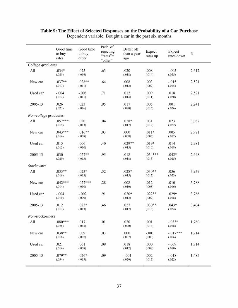
For households likely to have easier access to credit—those who graduated from college,
owned stocks, or owned homes—“good time-rates” is associated with a 3 to 4 percentage point
increase in the probability of purchasing a vehicle, and the marginal effect is not statistically
different from the effect of “good time-other” (table 9). For households who likely have more
tenuous access to credit—those who did not graduate from college, do not own stock, or do not
own a home—“good time-rates” is associated with a 6 to 8 percentage point increase in the
probability of buying a car. For all three groups with more-tenuous access to credit, the marginal
effect of “good time-rates” is statistically different from the effect of “good time-other.” The
effect of “rates-up” is statistically significantly different from zero for some types of households,
18
but the relationship between this variable and the likelihood of buying a vehicle does not vary in
a systematic way with the likelihood of being credit constrained.25
Turning to new and used car purchases, all types of households—both those more and
less likely to have easy access to credit— are about 4 percentage points more likely to purchase a
new car if they cited favorable auto credit conditions as a reason that car-buying conditions are
good six months earlier. However, scaling by the share of households in each group that
typically buy a new car in a given six-month period—which is about 3 percent for households
with more-tenuous access to credit and 7 percent for households with easier access to credit—
indicates that the purchases of households with more-tenuous access to credit are much more
sensitive to perceptions of credit conditions. Used-car purchases for all groups appear to be
unaffected by assessments of auto credit conditions.
As a robustness check, we excluded the 2003 and 2004 period from the subgroup
regressions. We found that the marginal effect of “good time-rates” declined but remained large
and significant for households who do not own stocks or houses; it was significantly different
from the effect of “good time-other” for households who do not own stock. As another
robustness check, we added month-date indicators to the models. This change resulted in only a
small decrease in the magnitude and statistical significance of the “good time-rates” and “rates-
up” coefficients (results not shown).
Discussion
Our analysis has assumed that variation in the “good time-rates” variable, after
controlling for other factors in the VAR and micro data specifications, captures changes in the
supply of auto credit. We showed that shocks to credit sentiment in the aggregate data move
together with the SLOOS measure of lender willingness to extend credit, which is consistent
with this interpretation.
Nonetheless, some of the changes in “good time-rates” that we have identified as supply
shocks may pick up other factors that are correlated with car purchases. For example,
households who are already inclined to purchase a vehicle may also be monitoring financing
25 The only discernible pattern with this coefficient is that it is more likely to be statistically significant when estimated over larger subgroups.
19
conditions more closely. We partly—but likely not completely—address this concern by
measuring perceptions in advance of vehicle purchases and by including a full suite of control
variables in the regression that capture some of the determinants of car purchases.
As an initial step towards exploring this possibility, we estimate a multivariate logit
model in which the three outcomes are: good time to buy a car because of credit conditions; good
time to buy a car for other reasons; and bad time to buy a car (table 10). The results indicate that
“good time-rates” is correlated with supply conditions: households are more likely to report this
answer when interest subvention is high. “Good time-rates” is also more prevalent among
households who live in a county where house prices have increased over the past year.26 This
result holds even controlling for county-level employment growth and the household’s perceived
change in its own house price over the past year, and it is consistent with the Mian, Rao, and Sufi
(2013) and Mian and Sufi (2014) findings that areas that saw the largest changes in house prices
also appear to have experienced larger changes in their ability to access credit.27
However, households that report favorable car-buying conditions because of low interest
rates are also more likely to have other characteristics that are associated with higher rates of
purchasing vehicles. For example, they tend to be younger and to have higher income. They are
more likely to report that they are better off financially than a year ago; that they expect higher
income in the future; and that the value of their house has increased during the past year.
Although we control for these variables in the regressions, these correlations raise the possibility
that “good time-rates” is capturing, in addition to credit supply changes, other differences across
households that are associated with car purchases.
More generally, our results raise several questions about consumer perceptions of car-
buying credit conditions and the relationship between this measure and vehicle purchases. For
example, how do households form their perceptions of auto financing conditions, and how
closely do these perceptions correspond with actual financing conditions? If perceptions and
reality differ, which is more important for vehicle purchases? How do these differences vary
26 A one-standard deviation increase in interest rate subvention is 0.5 and in the one-year house price change is 0.10. In both cases, a one-standard deviation shock is therefore associated with a 5 percentage point increase in the probability that a household reports “good time-rates.” 27 The county-level change in employment is from the Quarterly Census of Employment and Wages; the county-level change in house prices is from CoreLogic. The regression has a smaller sample size because the county level variables are not available for all households in the survey.
20
across groups? Does the strong relationship between interest subvention and vehicle purchases
reflect the effects of the advertising campaigns that generally accompany these promotions in
addition to the effects of low interest rates?
6. Conclusion
Consumer purchases of motor vehicles fell considerably during the 2007-09 recession,
and the decline in loan originations was even somewhat larger. In this paper, we showed that
significant swings in auto sales, auto loans, and credit availability are a regular feature of the
business cycle and that the drop in consumer vehicle purchases from 2007 to 2009, although the
largest decline in a long while, was about average relative to previous recessions. We then
demonstrated that changes in credit supply conditions are an important determinant of changes in
vehicle sales. One consistent finding from our work is that households who say “it’s a good time
to buy a car because interest rates are low” are significantly more likely to buy a new car some
months later. The effect is large and robust in both aggregate data and in household-level data,
even though the models we estimate for each type of data use different identification
assumptions, estimation techniques, and source data. The models are also estimated over
different time periods. The effect is large in both models relative to traditional determinants of
car purchases such as income and employment.
The results of the models are less consistent on some other fronts. For example, the VAR
estimates suggest a relationship between consumer perceptions of auto credit conditions and their
purchases of used cars; the household-level estimates do not. The household-level estimates
suggest a relationship between expectations of rising interest rates and car purchases; the VAR
estimates do not.
In the household-level data, we found evidence that perceptions of auto credit conditions
are particularly potent for the new vehicle purchases of households whose access to credit is
more likely to be tenuous—households without a college degree or who do not own stocks or
houses. This finding is consistent with the sharp decline in subprime loan originations during the
2007-09 recession and the subsequent rebound. We hesitate to draw too strong a linkage here,
though, as these households also likely faced greater exposure to other adverse shocks during
this period, such as unemployment.
21
REFERENCES
Aaronson, D., S. Agarwal, and E. French (2012). “The Spending and Debt Response to
Minimum Wage Hikes.” American Economic Review, 102(7): 3111-3139.
Adams, W., L. Einav and J. Levin (2009). “Liquidity Constraints and Imperfect Information in
Subprime Lending.” American Economic Review, 99(1): 49-84.
Attanasio, O., P. Goldberg and E. Kyriazidou (2008). “Credit Constraints in the Market for
Consumer Durables: Evidence from Micro Data on Car Loans.” International Economic Review,
49:2, 401-436.
Benmelech, E., R. Meisenzahl, and R. Ramcharan (2014). “Liquidity, Non-Bank Credit, and the
Financial Crisis: Evidence from Automobiles.” Working paper.
Campbell, S., D. Covitz, W. Nelson, and K. Pence (2011). “Securitization Markets and Central
Banking: An Evaluation of the Term Asset-Backed Securities Loan Facility.” Journal of
Monetary Economics, 58(5):518-531.
Chah, E., V. Ramey and R. Starr (1995). “Liquidity Constraints and Intertemporal Consumer
Optimization: Theory and Evidence from Durable Goods.” Journal of Money, Credit, and
Banking, 27:1, 272-287.
Covitz, D., N. Liang, and G. Suarez (2013). “The Evolution of a Financial Crisis: Collapse of
the Asset-Backed Commercial Paper Market.” Journal of Finance, 68:3, 815-848.
French, E., T, Kelley, and A. Qi (2013). “Expected Income Growth and the Great Recession.”
Federal Reserve Bank of Chicago Economic Perspectives, 37: 14-29.
Leininger, L., H. Levy, and D. Schanzenbach (2010). “Consequences of SCHIP Expansions for
Household Well-Being.” Forum for Health Economics and Policy, 13(1).
Mian, A., K. Rao, and A. Sufi (2013). “Household Balance Sheets, Consumption, and the
Economic Slump.” Quarterly Journal of Economics, 128(4): 1687-1726.
Mian, A., and A. Sufi (2014). “House Price Gains and U.S. Household Spending from 2002 to
2006.” Fama-Miller working paper, University of Chicago.
22
Ramcharan, R., S. Van den Heuvel, and S.Verani (forthcoming). “From Wall Street to Main
Street: The Impact of the Financial Crisis on Consumer Credit Supply.” Journal of Finance.
Sims, C. (1986). “Are Forecasting Models Usable for Policy Analysis?” Federal Reserve Bank of
Souleles, N. (1999). “The Response of Household Consumption to Income Tax Refunds.”
American Economic Review, 89(4): 947-58.
University of Michigan, Survey Research Center (2014). “Survey Description,” available on the
website of the Thomson Reuters/University of Michigan Surveys of Consumers
at www.sca.isr.umich.edu/survey-info.php (accessed March 16, 2014).
Van der Klaauw, W. (2012). “On the Use of Expectations Data in Estimating Structural
Dynamic Choice Models.” Journal of Labor Economics, 30(3): 521-554.
Wilcox, D. (1989). “Social Security Benefits, Consumption Expenditures, and the Life Cycle
Hypothesis.” Journal of Political Economy, 97: 288-304.
23
Figure 1: Real Personal Consumption Expenditures (PCE) 1967:Q1 through 2014:Q2
Notes. Data are from the National Income and Product Accounts. For each series x, the index is calculated as 100log log : .
Figure 2: Six-Quarter Changes in Real PCE for Durable Goods
1967:Q1 through 2014:Q2
Notes. Data are from the National Income and Product Accounts. Six quarters is the duration of the 2007-2009 recession.
1970 1975 1980 1985 1990 1995 2000 2005 2010-250
-200
-150
-100
-50
0
50Index (log change from 2007:Q4)
PCE motor vehiclesPCE excl. motor vehiclesPCE durable goods excl. motor vehicles & computers
1970 1975 1980 1985 1990 1995 2000 2005 2010-30
-20
-10
0
10
20
30
40
50Percent, ann. rate
PCE motor vehiclesPCE other durable goods
24
Figure 3: Auto Loan Originations 2000:Q1 through 2013:Q3
Notes. Data are from the Federal Reserve Bank of New York Consumer Credit Panel and from Equifax. Estimates were created by staff at the Federal Reserve Bank of Philadelphia and have been seasonally adjusted by the authors.
Figure 4: Auto Loan Originations by Credit Score Bucket
A. Number of Loan Originations
B. Loan Originations per 100 People
Notes. Data are from the Federal Reserve Bank of New York Consumer Credit Panel and from Equifax. Estimates were created by staff at the Federal Reserve Bank of Philadelphia and have been seasonally adjusted by the authors.
2006 2008 2010 2012 20140
2
4
6
8
10
12
14Millions of loans, ann. rate
2013:Q3
< 620620 to 659660 to 779
> 780Not reported
2006 2008 2010 2012 20146
8
10
12
14
16
18
20Millions of loans, ann. rate
< 620620 to 659660 to 779
> 780
26
Figure 5: Auto Loan Balances and Vehicle Collateral Value Index 1967:Q1 through 2013:Q4
Notes. Auto loan balances are from the Federal Reserve’s G.19 Consumer Credit release. The collateral value index of recently purchased vehicles is the discounted sum of nominal motor vehicle PCE in quarters leading up to and including the current date, assuming a 13 percent constant quarterly discount rate.
1970 1975 1980 1985 1990 1995 2000 2005 2010-30
-20
-10
0
10
20
304-quarter percent change
Loan balancesCollateral value index of recently purchased vehicles
27
Figure 6: Interest Rate Spreads for New Vehicle Loans 1976:Q1 to 2014:Q2
Notes. Spread is relative to the 2-year Libor swap rate. The interest rate for the captive finance companies reflects the average rate on loans originated by the finance arms of Ford, GM and Chrysler, and interest rate for commercial banks reflects the average rate on 48-month loans originated during the middle month of each quarter; both series are from the G.19 Consumer Credit statistics release published by the Federal Reserve Board (data for the finance companies were discontinued in February 2011). The interest rate for credit unions is from the Credit Union National Association. The interest rate for dealerships reflects the average rate on loans originated at dealerships from all types of lenders and is from the Power Information Network at J.D. Power & Associates. The 2-year swap rate is extrapolated prior to 2000 using the yield on 2-year Treasury notes.
Figure 7: Willingness of Domestic Banks to Make Consumer Installment Loans Senior Loan Officer Opinion Survey on Bank Lending Practices; 1966:Q3 to 2014:Q3
Notes. Figure shows the net percentage of domestic banks reporting an increased willingness to make loans.
Figure 8: Household Assessments of Auto Credit Conditions Reuters/University of Michigan Survey of Consumers; Jan. 1978 to Aug. 2014
Notes. Figure shows percentage of respondents to the Reuters/University of Michigan Survey of Consumers that cite low interest rates as reason that car-buying conditions are good less the percentage that cite high interest rates or tight credit conditions as reasons that car-buying conditions are bad.
Figure 9: Response of Real PCE for Motor Vehicles to Model Shocks Based on vector auto-regression; 1977:Q3 to 2007:Q4
Shock to real disposable personal income Shock to interest subvention
Shock to unemployment rate Shock to Real 2-year Swap Rate
Shock to Car-buying Credit Sentiment
Notes. Impulses are 1 standard deviation to the change in each explanatory variable. Responses in sales are cumulative sums of first differences. Dashed lines are 95% confidence bands.
30
Table 1: Growth of Real PCE for Durable Goods during Business Cycles
Notes. Data are from the National Income and Product Accounts. Recession dates are from the National Bureau of Economic Research.
Notes. The table reports the percentage of the variance of the error made in forecasting auto credit sentiment at the horizons shown in each row that is due to shocks to the variable listed at the top of each column.
Recessions(peak - trough)
Precedingpeak-to-peak
(Pct. change, a.r.)
Recession(Pct. change, a.r.)
Change(Pct. points)
1. 1969:4 - 1970:4 6.2 -6.7 -12.9 -12.8
2. 1973:4 - 1975:1 6.9 -7.1 -14.0 -6.8
3. 1980:1 - 1980:3 3.0 -13.2 -16.1 -11.5
4. 1981:3 - 1982:4 -1.5 1.0 2.5 3.1
5. 1990:3 - 1991:1 5.9 -10.6 -16.5 -11.5
6. 2001:1 - 2001:4 6.8 12.8 6.1 5.8
7. 2007:4 - 2009:2 6.0 -9.0 -15.1 -4.8
Memo:
Average
1967:1 ‐‐ 2007:4 5.5 -3.1 -8.7 -5.2
Real PCE Durable Goods Contribution of vehicle spending to
the change(Pct. points)
Interest subvention Interest rate DPI
PCE motor vehicles
Unempl. rate
Credit sentiment
1 0.70 15 2 0 6 1 75
4 0.78 10 17 1 12 7 52
8 0.80 10 17 2 13 8 50
Variance Decomposition(Percentage Points)
Forecast horizon
(Quarters)
Forecast standard error
31
Table 3: Michigan Survey Sample Sizes by Month
Dates of auto purchase and financing module
Number of households
Number of households who purchased autos
August 2003 204 31
February 2004 201 28
September 2004 203 43
April 2005 202 33
August 2005 200 31
December 2005 194 30
April 2006 200 26
August 2006 192 26
December 2006 196 24
April 2007 205 25
August 2007 193 33
December 2007 197 30
December 2008 196 20
February 2009 191 26
April 2009 195 24
August 2009 191 32
December 2009 195 22
February 2010 197 20
April 2010 196 16
August 2010 202 27
December 2010 194 23
April 2011 197 23
August 2011 202 25
December 2011 188 22
April 2012 206 23
August 2012 191 23
December 2012 187 25
April 2013 191 24
August 2013 193 20
Total 5,699 755
Note. Dataset derived from the Thomson Reuters / University of Michigan Survey of Consumers. Households in the sample are those in the given month who were also interviewed six months earlier. Households in which the respondent is someone other than the household head or spouse are excluded from the sample.
32
Table 4: Means of Selected Demographic Variables Michigan Survey and the Survey of Consumer Finances
Survey of Consumer Finances
Michigan Survey (cross-section)
Michigan Survey (panel)
Age 18-24 .05 .06 .05 Age 25-34 .16 .14 .12 Age 35-44 .19 .20 .19 Age 45-54 .21 .21 .21 Age 55-64 .17 .17 .18 Age 65+ .22 .22 .26 Income less than $35K .40 .30 .30 Income $35K-$60K .23 .21 .22 Income $60K-$100K .20 .22 .23 Income more than $100K .18 .20 .23 Income missing -- .06 .03 Married .51 .57 .59 White .73 .80 .82 Completed college .36 .42 .43 Stockowner .51 .64 .66 Homeowner .69 .79 .80
Notes. SCF data are from the 2004, 2007, and 2010 waves. SCF estimates are weighted with the x42001 weight and Michigan estimates are weighted with the household weight. Michigan (cross-section) refers to all households interviewed in months in which a vehicle financing module was conducted. Michigan (panel) refers to the subset of these households that had been interviewed six months earlier.
33
Table 5: The Effect of Selected Financing Conditions on the Probability of a Car Purchase Dependent variable: Bought a car in the past six months
Good time to buy—rates
Good time to buy—other
Prob. of rejecting “Rates” =“other”
Better off than a year ago
Expect rates up
Expect rates down
N
“Good time” only
.076***
(.015)
.028***
(.011)
.00 -- -- -- 5,699
“Rates up” only
-- -- -- -- .023**
(.010)
.006
(.017)
5,699
Better off” only
-- -- -- .054***
(.010)
5,699
All covariates .046***
(.014)
.023**
(.010)
.08 .024**
(.012)
.020**
(.009)
.009
(.016)
5,699
New cars .040***
(.011)
.022***
(.007)
.07 .004
(.007)
.007
(.005)
-.003
(.010)
5,502
Used cars .006
(.010)
.000
(.008)
.41 .022**
(.010)
.015**
(.007)
.014
(.013)
5,502
2003-07 .051**
(.021)
.002
(.017)
.01 .028
(.020)
.020
(.015)
-.034
(.027)
2,387
2008-13 .031*
(.018)
.037***
(.012)
.59 .020
(.017)
.019*
(.011)
.032
(.020)
3,312
2005-13 .028*
(.015)
.026**
(.010)
.94 .018
(.013)
.021**
(.010)
.022
(.018)
4,889
Date dummy variables
.040***
(.014)
.022**
(.010)
.17 .021*
(.012)
.021**
(.009)
.008
(.016)
5,699
Weighted .045***
(.015)
.021**
(.011)
.08 .020
(.013)
.014
(.010)
.006
(.017)
5,699
Notes. Dataset derived from the Thomson Reuters / University of Michigan Survey of Consumers. Each row shows selected marginal effects from a logit regression in which the dependent variable is “bought a car in the past six months,” with robust standard errors in parentheses. “Prob of reject rates=other” shows the confidence level at which we can reject the hypothesis that the “good time-rates” and “good time-other” coefficients are equal (based on a χ2 test). “New cars” and “used cars” show the marginal effects from a multinomial logit regression in which “buy a new car,” “buy a used car,” and “buy no car” are the outcomes. The sample size is smaller for this regression because the type of car question was not asked in the February 2010 survey. Significant at the *** 1 percent level, ** 5 percent level, * 10 percent level.
34
Table 6: Marginal Effects Estimates from the Main Logit Specification Dependent variable: bought a car in the past six months
Variable Marginal
effect Standard
error Financing conditions Good time to buy because of credit conditions .046*** .014 Good time to buy a car for other reasons .023** .010 Expect rates to go up
Expect rates to go down Two-year Libor swap rate Interest rate subvention
.020**
.009 .009 .016
-.001 .006 -.005 .021
Economic conditions Better off financially than a year ago .024** .012 Worse off financially than a year ago .005 .011 Expect higher family income--next 12 months
Expect lower family income--next 12 months .003 .011
-.014 .012 Current house value is higher relative to a
year ago .004 .011
Current house value is lower relative to a year ago
-.001 .012
Demographics Age 18-34 .095*** .025 Age 35-44 .067*** .020 Age 45-54 .078*** .017 Age 55-64 .043*** .016 Income $35,000 - $60,000 .038** .017 Income $60,000 - $100,000 .052*** .018 Income greater than $100,000 .043** .019 Income missing .004 .028 White .027** .011 Married .052*** .010 Attended college -.018* .009 Own stock -.008 .011 Own home .005 .014 R-squared .04 N 5,699
Notes. Dataset derived from the Thomson Reuters / University of Michigan Survey of Consumers. Robust standard errors are shown. Significant at the *** 1 percent level, ** 5 percent level, * 10 percent level.
35
Table 7: Michigan Sample Summary Statistics
Variable Mean Standard Deviation
Bought a car in the past six months 0.13 0.34 Financing conditions Good time to buy a car because of credit
conditions 0.20 0.40
Good time to buy a car for other reasons 0.43 0.50 Expect rates to go up
Expect rates to go down Two-year Libor swap rate Interest rate subvention
0.53 0.50 0.10 0.30 2.44 1.74 1.14 0.50
Economic conditions Better off financially than a year ago 0.30 0.46 Worse off financially than a year ago 0.42 0.49 Expect higher family income--next 12 months
Expect lower family income--next 12 months 0.50 0.50 0.20 0.45
Current house value is higher relative to a year ago
0.29 0.45
Current house value is lower relative to a year ago
0.26 0.44
Demographics Age 18-34 0.10 0.30 Age 35-44 0.17 0.37 Age 45-54 0.23 0.42 Age 55-64 0.22 0.41 Age 65+ 0.28 0.45 Income less than $35,000 0.26 0.44 Income $35,000 - $60,000 0.22 0.41 Income $60,000 - $100,000 0.25 0.43 Income greater than $100,000 0.24 0.43 Income missing 0.04 0.19 White 0.84 0.36 Married 0.62 0.49 College graduate 0.46 0.50 Own stock 0.69 0.46 Own home 0.83 0.37
Notes. Dataset derived from the Thomson Reuters / University of Michigan Survey of Consumers. Statistics are unweighted.
36
Table 8: Selected Means by Subgroup
All College graduate
Non-graduate
Stock-owner
Non-stock-owner
Home-owner
Renter
----------------- Survey of Consumer Finances -----------------
Turned down for credit
.28 .20 .33 .14 .31 .21 .44
Ever late on a loan payment
.18 .13 .21 .10 .20 .15 .26
… 60 days late .07 .05 .08 .03 .08 .05 .10
Purchased a car .17 .17 .17 .18 .17 .18 .15
… new car .06 .08 .04 .09 .05 .07 .02
… … w/a loan .70 .66 .74 .52 .77 .68 .82
… used car .12 .09 .13 .09 .13 .11 .13
… … w/a loan .35 .38 .34 .34 .35 .37 .32
----------------- Michigan Survey of Consumers -----------------
Purchased a car .13 .15 .12 .15 .12 .13 .11
… new car .05 .07 .04 .06 .04 .06 .02
… used car .08 .08 .08 .08 .08 .08 .08
Notes. The SCF means are calculated with data from the 2004, 2007, and 2010 waves of the Survey of Consumer Finances and are weighted. A household is considered “turned down for credit” if, at any point in the past five years, it was turned down for credit; did not get as much credit as requested; or did not apply because of a concern of being rejected for the loan. “Ever late on a loan payment” and “60 days late” refer to the household’s experience in the previous year. In the SCF data, the car purchase variables are the share of households who purchased a car in the previous 9 months or so. In the Michigan data, the car purchases refer to the previous 6 months. The Michigan estimates are weighted and are based on all households surveyed in the months in which the vehicle module was conducted.
37
Table 9: The Effect of Selected Responses on the Probability of a Car Purchase Dependent variable: Bought a car in the past six months
Good time to buy—rates
Good time to buy—other
Prob. of rejecting “rates”= “other”
Better off than a year ago
Expect rates up
Expect rates down
N
College graduates
All .034* (.021)
.025 (.016)
.63 .020 (.018)
.008 (.014)
-.005 (.025)
2,612
New car .037** (.017)
.028** (.011)
.64 .008 (.012)
.003 (.009)
-.015 (.015)
2,521
Used car
-.004 (.012)
-.008 (.011)
.71 .012 (.014)
.009 (.011)
.018 (.020)
2,521
2005-13 .026 (.023)
.023 (.016)
.95 .017 (.020)
.005 (.016)
.001 (.026)
2,241
Non-college graduates
All .057*** (.019)
.020 (.013)
.04 .028* (.017)
.031 (.012)
.023 (.022)
3,087
New car .043*** (.014)
.016** (.008)
.03 .000 (.008)
.011* (.006)
.005 (.012)
2,981
Used car .015 (.013)
.006 (.010)
.40 .029** (.015)
.019* (.010)
.014 (.018)
2,981
2005-13 .030 (.020)
.027** (.013)
.95 .018 (.018)
.034*** (.013)
.042* (.025)
2,648
Stockowner
All .033** (.016)
.023* (.013)
.52 .028* (.015)
.030** (.012)
.036 (.023)
3,939
New car .042*** (.014)
.027*** (.010)
.28 .008 (.010)
.012 (.008)
.010 (.016)
3,788
Used car -.004 (.010)
-.002 (.009)
.91 .020* (.012)
.022** (.009)
.029* (.018)
3,788
2005-13
.012 (.017)
.023* (.013)
.46 .027 (.017)
.030** (.013)
.043* (.024)
3,404
Non-stockowners
All .080*** (.028)
.017 (.015)
.01 .020 (.020)
.001 (.014)
-.033* (.018)
1,760
New car .038** (.016)
.009 (.007)
.03 .000 (.007)
-.001 (.006)
-.017*** (.006)
1,714
Used car .021 (.014)
.001 (.008)
.09 .018 (.012)
.000 (.008)
-.009 (.010)
1,714
2005-13 .079** (.034)
.026* (.015)
.09 -.001 (.020)
.002 (.015)
-.018 (.022)
1,485
38
Table 9, continued
Good time to buy—rates
Good time to buy—other
Prob. of rejecting “rates” = “other”
Better off than a year ago
Expect rates up
Expects rates down
N
Homeowners
All .042*** (.015)
.024** (.011)
.19 .023* (.014)
.019* (.010)
.016 (.019)
4,745
New car .039*** (.012)
.025*** (.008)
.24 -.001 (.008)
.008 (.006)
-.004 (.011)
4,572
Used car .004 (.010)
-.003 (.008)
.42 .026** (.012)
.014* (.008)
.020 (.015)
4,572
2005-13 .022 (.016)
.023** (.012)
.88 .016 (.015)
.019* (.011)
.023 (.020)
4,127
Renters
All .070** (.034)
.017 (.020)
.08 .034 (.028)
.022 (.020)
-.019 (.030)
954
New car .036** (.018)
.003 (.009)
.02 .024 (.016)
.003 (.008)
.001 (.012)
930
Used car .017 (.018)
.008 (.011)
.56 .002 (.014)
.012 (.011)
-.011 (.016)
930
2005-13 .072** (.045)
.032 (.020)
.37 .032 (.032)
.026 (.022)
.013 (.042)
762
Notes. Each row shows selected marginal effects from a logit regression in which the dependent variable is “bought a car in the past six months,” with robust standard errors in parentheses. “Prob of reject rates=other” shows the confidence level at which we can reject the hypothesis that the “good time-rates” and “good time-other” coefficients are equal (based on a χ2 test). “New cars” and “used cars” show the marginal effects from a multinomial logit regression in which “buy a new car,” “buy a used car,” and “buy no car” are the outcomes. The sample size is smaller for this regression because the type of car question was not asked in the February 2010 survey. Significant at the *** 1 percent level, ** 5 percent level, * 10 percent level.
39
Table 10: Characteristics of Households by Car-Buying Attitudes (Marginal Effects from a Multinomial Logit)
Dependent variable: Is it a good time to buy a car?
Current house value is higher than a year ago .038** (.017)
.013 (.021)
-.025 (.020)
Current house value is lower than a year ago -.028* (.015)
-.009 (.021)
.019 (.020)
Better off financially than a year ago .047*** (.016)
.027 (.020)
-.021 (.020)
Worse off financially than a year ago -.004 (.014)
-.054*** (.018)
.058*** (.018)
Expect higher family income--next 12 months .024* (.014)
-.009 (.018)
-.033* (.018)
Expect lower family income--next 12 months -.036** (.016)
.041* (.021)
.077*** (.021)
Expect rates to go up -.000 (.012)
-.025 (.016)
.026 (.016)
Expect rates to go down .014 (.021)
-.059** (.026)
.045* (.026)
Demographics Age 18-34 .078***
(.027) -.132*** (.027)
.055* (.030)
Age 35-44 .091*** (.023)
-.133*** (.023)
.042* (.025)
Age 45-54 .069*** (.020)
-.110*** (.021)
.040* (.022)
Age 55-64 .034* (.019)
-.060*** (.021)
.027 (.021)
Income $35,000 - $60,000 .046** (.021)
.002 (.024)
-.048** (.021)
Income $60,000 - $100,000 .047** (.022)
.038 (.025)
-.085*** (.023)
40
Variable Good time to buy a car-interest rates
Good time to buy a car-other reason
Bad time to buy a car
Income greater than $100,000
.057** (.024)
.044 (.027)
-.100*** (.025)
Income missing -.045 (.031)
.024 (.042)
.021 (.040)
White .046*** (.014)
-.019 (.021)
-.027 (.020)
Married .001 (.013)
-.015 (.021)
.014 (.017)
Attended college -.009 (.012)
.033** (.016)
-.024 (.020)
Own stock .050*** (.014)
.019 (.019)
-.068*** (.018)
Own home .015 (.018)
-.002 (.025)
-.013 (.017)
R-squared .05 N 4,913
Notes. The table shows marginal effects from a multinomial logit regression in which the dependent variable is “Is it a good time to buy a car?” Each column shows the results for a different outcome value. The sample size is smaller than in the other regressions because county-level data are not available for all households. Dataset derived from the Thomson Reuters / University of Michigan Survey of Consumers. Robust standard errors are shown. Significant at the *** 1 percent level, ** 5 percent level, * 10 percent level.