Highlights We propose a new methodology to estimate the long-run elasticity between growth and finance. The contemporaneous relationship between financial booms and economic growth is positive for a complete growth cycle, even if high financial growth makes recessions more severe. Financial booms have however a persistent effect detrimental to subsequent cycles, which is referred as a hysteresis phenomenon. We define the threshold of financial development above which the persistent effect dominates the contemporaneous effect. The total effect of finance on growth is negative as this threshold is exceeded in our panel of economies. Finance and Growth: From the Business Cycle to the Long Run No 2016-28 – December Working Paper Thomas Grjebine & Fabien Tripier
Transcript
Highlights
We propose a new methodology to estimate the long-run elasticity between growth and finance.
The contemporaneous relationship between financial booms and economic growth is positive for a complete growth cycle, even if high financial growth makes recessions more severe.
Financial booms have however a persistent effect detrimental to subsequent cycles, which is referred as a hysteresis phenomenon.
We define the threshold of financial development above which the persistent effect dominates the contemporaneous effect.
The total effect of finance on growth is negative as this threshold is exceeded in our panel of economies.
Finance and Growth: From the Business Cycle to the Long Run
No 2016-28 – December Working Paper
Thomas Grjebine & Fabien Tripier
CEPII Working Paper Finance and Growth: From the Business Cycle to the Long Run
Abstract This paper proposes a new methodology to assess the long-run relationship between economic and financial growth. By linking long-run growth to the properties of business cycles, this methodology offers a better understanding of the channels through which finance can impact long-term growth. We first define the direct elasticity between financial and economic growth to measure the contemporaneous effect of financial growth. If financial booms make recessions more severe, losses of growth during recessions are low when compared with growth supplements during expansions. Beyond this contemporaneous effect of financial booms, we identify a persistent effect of financial growth detrimental to subsequent cycles, which is referred as a hysteresis phenomenon. Then, financial and economic growth rates are positively correlated only up to a certain threshold of financial activity. In our panel of economies, the average level of financial activity is well above this threshold, implying that the total elasticity between finance and growth is negative in the long run.
KeywordsGrowth, Business Cycles, Hysteresis, Financial Cycles, Growth Cycles.
JELE32, E44.
CEPII (Centre d’Etudes Prospectives et d’Informations Internationales) is a French institute dedicated to producing independent, policy-oriented economic research helpful to understand the international economic environment and challenges in the areas of trade policy, competitiveness, macroeconomics, international finance and growth.
CEPII Working PaperContributing to research in international economics
CEPII Working Paper Finance and Growth: From the Business Cycle to the Long Run
Finance and Growth: From the Business Cycle to the Long Run
Thomas Grjebine,∗ and Fabien Tripier†
"How long has it been since the American economy enjoyed reasonable growth, from a rea-sonable unemployment rate, in a financially sustainable way? The answer is that is has beenreally quite a long time, certainly more than half a generation". Summers (2015)
"We may be an economy that needs bubbles just to achieve something near full employment".Krugman (2013)
1. Introduction
The "Secular Stagnation" debate launched by Summers (2013) and Krugman (2013) has recentlyrevived the attention on the difficulties to conciliate economic growth with financial stability. Theyraise in particular the question of what would have been growth during the last thirty years indeveloped economies without financial and housing bubbles. This debate highlights the complexityof the interactions between economic growth and finance, which has been alternatively pointed outas a key driver of economic growth and a major source of amplification of economic crisis. Thispaper proposes a new empirical methodology which provides a unified framework to estimate andcompare these different effects throughout and across business cycles.
This novel framework uncovers three new important patterns. First, even if high financial growth1makes recessions more severe, the elasticity between finance and growth for a complete businesscycle is found on average positive. Second, this positive elasticity should be adjusted downward bythe excessive development of finance inherited from previous cycles, which is referred as a hysteresisphenomenon. Third, there is a threshold of financial activity above which the elasticity betweenfinance and growth becomes negative in the long run, i.e. over several cycles, because of thehysteresis effects of financial growth.
Our methodology allows to synthesize in a unified framework two strands of the literature on growthand finance. A large empirical literature on long-run growth has been developed in the traditionof King and Levine (1993) after the precursory contributions of Goldsmith (1969) and McKinnon(1973). The starting point of this literature is to regress long-run growth for a panel of country on aset of variables among which one of them measures the development of the financial sector and the∗CEPII ([email protected])†Univ. Evry – EPEE and CEPII ([email protected])1Financial growth refers to the growth rate of financial series (as house prices) and indicators of financial development(as credit to GDP ratio).
CEPII Working Paper Finance and Growth: From the Business Cycle to the Long Run
other are control variables. This literature concluded on the existence of a positive and significantrelationship between average growth and various measures of financial activity – see among othersLevine (1997), Benhabib and Spiegel (2000) and Beck et al. (2007) – even if recent studies havechallenged the robustness of this conclusion as Cecchetti and Kharroubi (2012), Rousseau andWachtel (2011, 2015) or Arcand et al. (2015). To take into account the time-varying behavior of thefinancial sector, these studies estimate dynamic panels using window of several years (generally fiveyears) to eliminate business cycle fluctuations. Another recent literature focuses precisely on businesscycle fluctuations to identify the links between financial activity and economic crisis. Actually, they donot consider all business cycle fluctuations, but they focus instead on the recessions’ characteristics,that is the probability of occurrence, the severity, and the duration. Drehmann et al. (2012) showthat financial cycle peaks are very closely associated with financial crises and business cycle recessionsare much deeper when they coincide with the contraction phase of the financial cycle; Claessenset al. (2012) that the duration and amplitude of recessions are higher when they occur with financialdisruptions; Jordà et al. (2013) that the severity of recessions is amplified by the intensity of financialdevelopment2; and Schularick and Taylor (2012) that the credit ratio is a good predictor of financialcrisis3. In this literature, less attention is given to economic expansions, which however determinethe long-run growth when cumulated over the cycles of an economy.
To sum up, the literature on growth does not consider the specificity of business cycle phases whilethe literature on recessions does not take into account the economic growth process associated withthe expansion phases. In this article, we fill the gap between these two strands of the literatureby providing a unified empirical framework. By doing so, we complement recent attempts in theliterature to balance the various interactions between finance and growth by Ranciere et al. (2006),Loayza and Ranciere (2006), Bonfiglioli (2008), and Rancière and Tornell (2016).4 The key point ofour approach is that we do not split series into trend and cyclical components by removing a trendfrom original series to get the cyclical fluctuations. Instead, we study the classical business cyclewhich is defined by the analysis of turning points (known as peaks and troughs) between expansionand recession phases – see Stock and Watson (1999).5 The interest of this set-up is to link thelong-run economic growth to the properties of business cycles. Indeed, the long-run growth of an2See also Mian et al. (2015) who show that an increase in the household debt to GDP ratio over a three year periodpredicts lower GDP growth over the next three years. They depart from the above literature as their results are notconditional on having a recession.3See also Borio et al. (2013) who develop measures of potential output and output gaps in which financial factorsplay a central role.4Ranciere et al. (2006) develop a setup to decompose the effects of financial liberalization on economic growthand on the incidence of crises. To do so, they introduce crisis events into standard growth regressions augmentedwith financial variables. Loayza and Ranciere (2006) propose an estimation of the short- and long-run impacts offinancial intermediation using the Pooled Mean Group estimator developed by Pesaran et al. (1999). They finda positive long-run relationship between financial intermediation and output growth that co-exists with a mostlynegative short-run relationship. In a similar manner, Bonfiglioli (2008) studies the effects of financial globalizationon investment and productivity growth by controlling for indirect effects on banking and currency crisis. Rancièreand Tornell (2016) develop a two-sector model consistent with these empirical facts in which financial liberalizationmay increase growth, but leads to more crises and costly bailouts.5Gadea Rivas and Perez-Quiros (2015) study the relations between credit and growth both during expansion and
4
CEPII Working Paper Finance and Growth: From the Business Cycle to the Long Run
Table 1 – Results: Summary table
Growth Channel Duration Channel TotalEffects of (1) (2) (3) (4) (5) (6) (7)Excess Finance Expansion Recession Cycle Expansion Recession Cycle Total(a) Direct effect + − + + 0∗ + +(b) Persistent effect − − − 0∗ 0∗ 0∗ −(c) Total effect + − − + 0∗ + −This table summarizes our results for the six measures of excess finance. ∗ indicates that we get adifferent result for at least one of the six variables.
economy is equal to the average growth observed for all business cycles of this economy. We showthat the elasticity between growth and finance can be expressed as the sum of elasticities associatedwith the business cycle properties. By linking long-run growth to the properties of business cycles,this methodology offers a better understanding of the channels through which finance can impactlong-term growth.
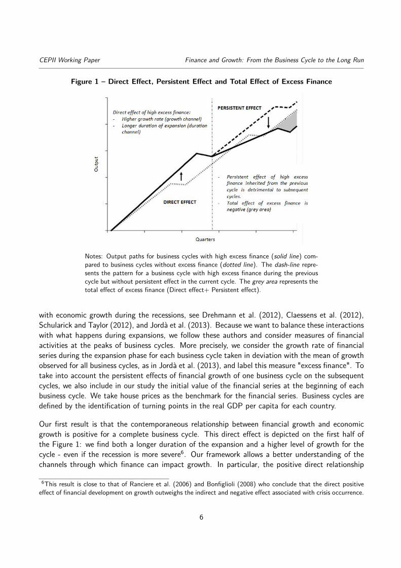
The channels through which finance can impact long-term growth are investigated at two levels,which are summarized in Table 1 and Figure 1 – the solid line corresponds to the economic activitywhen financial growth is high, while the dotted line is the level of output when the financial growth isequal to its mean-value in the sample. The first level of analysis corresponds to the contemporaneouseffect of financial growth on a complete business cycle, composed of one expansion and one recession,which is interpreted as the direct effect – the line (a) of the Table 1 and the first half of the Figure 1.Finance-growth interactions are the result of two channels : (i) the growth channel, associated withthe difference in the growth rates between the expansion and recession phases, and (ii) the durationchannel, associated with the difference in the durations of the expansion and recession phases.
The second level of analysis corresponds to the interdependencies between business cycles, throughthe persistent effects of financial growth on the initial value of financial series for subsequent cycles– the line (b) of the Table 1 and the second half of the Figure 1. We refer to this phenomenonas hysteresis because the consequences of a high financial growth episode can persist even if highfinancial growth has stopped – see Blanchard et al. (2015) and Gali (2016) for recent contributionson the importance of the concept of hysteresis to understand the full consequences of recessions.This can also be related with the concept of "Debt Supercycle" developed by Rogoff (2015) accordingto which the inheritance of excessive development of finance in the past can lead to long-lastinglow economic growth. The total effect of financial growth is computed as the sum of direct andpersistent effects – the line (c) of the Table 1.
Our methodology is applied to a panel of 26 countries over the period 1970-2015. The applicationof this methodology requires an empirical measure for finance. The recent empirical literature usesmeasures of financial activities around the peaks of economic activity to assess their interactions
recession phases, as we do, but with a different objective. The authors’ objective is to assess the ability of credit-basedindicators to forecast efficiently the recessions. They show the poor performances of credit-based indicators in outof sample prediction of crisis because of the procyclical behavior of credit, which increases during expansion.
5
CEPII Working Paper Finance and Growth: From the Business Cycle to the Long Run
Figure 1 – Direct Effect, Persistent Effect and Total Effect of Excess Finance
Notes: Output paths for business cycles with high excess finance (solid line) com-pared to business cycles without excess finance (dotted line). The dash-line repre-sents the pattern for a business cycle with high excess finance during the previouscycle but without persistent effect in the current cycle. The grey area represents thetotal effect of excess finance (Direct effect+ Persistent effect).
with economic growth during the recessions, see Drehmann et al. (2012), Claessens et al. (2012),Schularick and Taylor (2012), and Jordà et al. (2013). Because we want to balance these interactionswith what happens during expansions, we follow these authors and consider measures of financialactivities at the peaks of business cycles. More precisely, we consider the growth rate of financialseries during the expansion phase for each business cycle taken in deviation with the mean of growthobserved for all business cycles, as in Jordà et al. (2013), and label this measure "excess finance". Totake into account the persistent effects of financial growth of one business cycle on the subsequentcycles, we also include in our study the initial value of the financial series at the beginning of eachbusiness cycle. We take house prices as the benchmark for the financial series. Business cycles aredefined by the identification of turning points in the real GDP per capita for each country.
Our first result is that the contemporaneous relationship between financial growth and economicgrowth is positive for a complete business cycle. This direct effect is depicted on the first half ofthe Figure 1: we find both a longer duration of the expansion and a higher level of growth for thecycle - even if the recession is more severe6. Our framework allows a better understanding of thechannels through which finance can impact growth. In particular, the positive direct relationship
6This result is close to that of Ranciere et al. (2006) and Bonfiglioli (2008) who conclude that the direct positiveeffect of financial development on growth outweighs the indirect and negative effect associated with crisis occurrence.
6
CEPII Working Paper Finance and Growth: From the Business Cycle to the Long Run
between finance and growth – column (7) on line (a) of the Table 1 – does not only come fromhigher growth rates but also from longer duration of expansions – columns (3) and (6) on line(a) of the Table 1. For example, for house prices, the total elasticity is equal to 3.4%7. Thiselasticity is the sum of the elasticities linked to the growth channel (3.1%) and the duration channel(0.3%). Looking at the growth channel, the elasticity is positive during the expansion (5%) andturns negative during the recession phase (-1.9%).8
However, this result does not take into account the persistent effects of excess finance on subsequentcycles through the initial value of financial series. Actually, our second result is that the relationshipbetween the initial value of the financial series at the beginning of a business cycle and the economicgrowth during this cycle is negative – column (7) on line (b) of the Table 1. This persistent effectis depicted on the second half of Figure 1: the solid line crosses back the dotted line quickly afterthe beginning of the subsequent cycle and remains below. The bold dotted line plots the level ofoutput with high financial growth when hysteresis effects are not accounted for. It gives a graphicalintuition for our novel finding that finance is detrimental over the long run: hysteresis effects of highfinancial growth reduce the slope of the subsequent cycles.
To sum up, financial growth is positively related with economic growth - through the direct effect– and negatively – through the persistent effect. We compute the threshold of financial activityabove which the persistent effect outweighs the direct effect, making financial growth detrimentalto economic growth. In our sample of economies, the average level of financial activity is well abovethis threshold, implying a negative elasticity between finance and growth9 – hence the negative signon line (c) for the Total effect in Table 1. For example, for house prices, this elasticity is equal to−2.7%, which is the sum of the 3.4% for the direct elasticity and the −6.1% associated with thepersistent effects.
For robustness, we show that our regression results are roughly the same for five other measuresof excess finance – the Price-to-Rent ratio, Real Credit, Credit to GDP, Real Households Credit,Households Credit to GDP – and when properties of the financial cycle are explicitly taken intoaccount – as the occurrence of bank crisis. We show also that our results are robust to controllingfor endogeneity as recently suggested by Arcand et al. (2015).10 We finally test the hypothesis thatthe hysteresis effect could come from the link between finance and productivity as financial boomscould affect negatively productivity with long-term consequences on economic growth.
The rest of the paper proceeds as follows. In Section 2, we describe the empirical methodology. In7This number should be interpreted as follows: a 1% excess finance is associated in the data with a variation of
0.03 points of percentage of GDP quarterly growth.8The sum of these two elasticities is the value of the growth channel (3.1%).9In average for our six measures of excess finance, this threshold corresponds to a third of the level of the financialseries observed in our sample in 2014-2015.10Following Arcand et al. (2015), we control for endogeneity of our regression models using the estimators developedby Rigobon (2003) and Lewbel (2012) that allow to identify causal relationships through heteroskedasticity. In thepresence of heteroskedasticity in the regression’s residual, this methodology allows identifying causal relationshipseven in the absence of external instruments.
7
CEPII Working Paper Finance and Growth: From the Business Cycle to the Long Run
Section 3, we present the data. In Section 4, we show the results and we propose simulations ofGDP patterns depending on variations in excess finance. In Section 5, we propose robustness checksby using alternative measures of finance, controlling for endogeneity and for the financial cycle.
2. Methodology
This section describes the empirical methodology (calculus details are provided in Appendix C).
2.1. Business Cycles and Excess Finance
We consider a panel of n countries indexed by i = 1, ..., n where Ti is the number of observationsof the series for the country i. To implement our methodology, the series should be defined in thedimension of economic cycles and not only in the time domain. For each country i, we observec = 1, ..., Ci cycles. For each cycle c, s = 1, ..., τc stands for the quarter of the cycle and τc forthe duration of the cycle. In the cycle dimension, Yi,c,s denotes the real GDP per capita observedduring the quarter s of the cycle c in country i, which quarterly growth rate is denoted gi,c,s ≡log (Yi,c,s/Yi,c,s−4) /4. The cycle c can itself be decomposed into two business cycle phases: theexpansion and the recession. In the remainder, we use the following notation: xph refers to the valueof the series x for the business cycle phase ph, which can take two values ph = {ex, re} where exstands for expansion and re for recession. The duration of the business cycle satisfies τc = τ exc + τ recwhere τ exc is the duration of the expansion phase and τ rec the duration of the recession phase. Thepeak of a typical business cycle is reached as of time τ exc , which is the end of the expansion phaseand the beginning of the recession phase, one quarter after. The trough of the cycle correspondsto the period (τ exc + τ rec ) , which is the end of the recession and the start of the next cycle, onequarter after. The phase ph represents the share πph = τ phc /τc of the duration of the cycle c forph = {ex, re} .
The average growth rate of the real GDP for the panel of countries is denoted g and defined asg ≡ 1
n
∑ni=1 gi, where gi denotes the average growth for the economy i. The interest of the cycle
dimension is to take into account potential differences between expansion and recession businesscycle phases. To do so, we consider the growth rate for the cycle c in country i, which is denotedgi,c and defined as follows
gi,c ≡ πexi,cgexi,c + πrei,cg
rei,c (1)
It is the average of the growth rates during the expansion and recession phases, respectively denotedgexi,c and grei,c, weighted by the share of each business cycle phase in the full duration of the cycle,namely πex and πre respectively. The averages of growth rates for each business cycle phase aredefined as follows
gexi,c ≡1τ exi,c
τexi,c∑s=1
gexi,c,s, and grei,c ≡1τ rei,c
τi,c∑s=τex
i,c+1grei,c,s (2)
These definitions of growth are used hereafter to compute the elasticity of growth with respect tofinancial series.
8
CEPII Working Paper Finance and Growth: From the Business Cycle to the Long Run
As for the real GDP per capita, we define financial series in the cycle dimension: Fi,c,s denotes thevalue of the financial series F measured for the quarter s of the cycle c in country i. We do notconsider herein the specific cycles of the financial series – in Section 5 we consider explicitly thefinancial cycle as robustness checks. Then, the timing of expansion and recession of business cyclephases is the same as for the real GDP per capita. Actually, we are interested by the properties ofbusiness cycles in terms of financial activities. For each financial series, we consider its initial valueat the beginning of each business cycle
φ0i,c ≡ Fi,c,0 (3)
and its excess growth during the expansion phase
φexi,c ≡ log(Fi,c,τex
i,c/Fi,c,0
)/τ exi,c − φ̄ex (4)
which is the quarterly average growth rate of the financial series during the expansion phase indeviation with respect to φ̄ex, the average of growth rates for all the cycles of all the countries ofthe panel, namely
φ̄ex ≡ (1/n)n∑i=1
(1/Ci
) Ci∑c=1
log(Fi,c,τex
i,c/Fi,c,0
)/τ exi,c (5)
where Ci represents the number of cycles observed for the economy i.
2.2. The Direct Elasticity between Growth and Excess Finance
The direct elasticity refers to the relationship between growth and excess finance for one typicalbusiness cycle without taking into account the interdependencies between business cycles.
Our methodology considers the elasticity between excess finance and growth to characterize theinteractions between these two variables. To be more explicit, we are interested in the (semi-)elasticity11 of the growth rate gi,c with respect to the measure of excess finance φexi,c during thecycle c in country i, which is given by the following first order partial derivative
εDφexi,c≡ ∂gi,c∂φexi,c
(6)
Using the definition of gi,c provided by (1), the elasticity defined by (6) is equal to
εDφexi,c
=∂gexi,c∂φexi,c
πexi,c +∂grei,c∂φexi,c
πrei,c +(∂τ exi,c∂φexi,c
τ rei,c −∂τ rei,c∂φexi,c
τ exi,c
)gexi,c − grei,c(τ exi,c + τ rei,c
)2 (7)
We use two regression with two different dependent variables to quantify the terms present in theequation (7). First regressions consider the growth rate during business cycle phases as a dependent11 Since both gi,c and φexi,c are the log of "gross" growth rates of real GDP per capita and the financial series, εgφex
is the semi-elasticity between these two rates and the elasticity between these two "gross" rates. For simplicity, weuse the term elasticity for in the remainder while keeping in mind that it concerns the "gross" rates of series.
9
CEPII Working Paper Finance and Growth: From the Business Cycle to the Long Run
variable and the second regressions consider the duration of business cycle phases as a dependentvariable.
Growth regressions are estimated with the OLS estimator with fixed effects using the followingspecification
gphi,c,s = cphg + fphg,i + αphg φexi,c + βphg φ
0i,c + γphg X
gi,c,s + εi,c,s (8)
for each phase ph = {ex, re} . In this regression, cphg is the constant term, fphg,i a country-fixedeffect, Xg
i,c,s is a set of controls for both business cycles and growth, and αphg the coefficient ofinterest that measures the elasticity between growth and excess finance during the business cyclephase ph = {ex, re}. We discuss below the consequences of the initial value of the financial series,associated with the coefficient βphg , in terms of persistence. Using, (8) the elasticity of growth withrespect to excess finance during the business cycle phase ph writes
∂gphi,c∂φexi,c
= 1τ phi,c
τphi,c∑s=1
∂gphi,c,s
∂φphi,c= 1τ phi,c
τphi,c∑s=1
αphg = αphg (9)
for ph = {ex, re} .
For duration regressions, we use a parametric hazard model. The hazard is the probability of exitingfrom a state (for example, a recession or an expansion) conditional on the length of time in thatstate. Hazard models have been initially applied to the duration of business cycles by Sichel (1991)to assess whatever business cycles exhibit a positive duration dependence – in this case, periodsof expansion or recession are more likely to end as they become older. Recently, Claessens et al.(2012) have extended this methodology to consider fixed effects and the influence of other variablesfor the probability of exiting from a business cycle phase. We then follow Claessens et al. (2012) toassess whatever our financial series influence the durations of recessions and expansions. Assumingthat the duration τ phi,c of the business cycle phase ph = {ex, re} has a Weibull distribution12, thelogarithm of duration τ phi,c can be estimated using the following specification13
log(τ phi,c
)= cphτ + fphτ,i + αphτ φ
exi,c + βphτ φ
0i,c + γphg X
τi,c + zphi,c (10)
where zphi,c has an extreme-value distribution scaled by the inverse of the shape parameter of theWeibull distribution, denoted pph. In this regression, cphτ is the constant term, fphτ,i a country-fixed12There is a great variety of parametric duration models, with the Weibull model the most commonly used for businesscycle studies– see Diebold et al. (1993) for alternative specifications. The fundamental assumption of the Weibullmodel is a linear relationship between the log of the hazard function and the log of duration since the functionalform for the hazard is h(t) = ptp−1 where t is duration of the phase and p the Weibull parameter - there is positiveduration dependence for p > 1.13The assumption of a linear relationship between the log of duration and explanatory variables (both fixed effectsand control variables) corresponds to the Accelerated Failure Time (AFT) specification of duration models withtime-varying covariates; the alternative is the Proportional Hazard (PH) specification with multiplicative effects - seeJenkins (2005) for a discussion.
10
CEPII Working Paper Finance and Growth: From the Business Cycle to the Long Run
effect, Xτi,c is a set of controls for both business cycles and growth, and αphτ the coefficient of interest.
Using (10), the (semi-)elasticity of the duration of the business cycle phase ph with respect to excessfinance is
∂τ phi,c∂φexi,c
= αphτ τphi,c (11)
for ph = {ex, re}.
The average value of εDφexi,c, defined by (7) for all the panel, is therefore
εDφex = 1n
n∑i=1
1Ci
Ci∑c=1
[αexg π
exi,c + αreg π
rei,c + (αexτ − αreτ ) πexi,cπrei,c
(gexi,c − grei,c
)](12)
given the outcomes of the regressions (8) and (10). In the remainder, we use the variable σi,c ≡πexi,cπ
rei,c
(gexi,c − grei,c
), which provides a measure of the gap in growth rates between the two business
cycle phases, namely (gexi,c − grei,c), weighted by the relative duration of business cycle phases, πexi,cand πrei,c. Then, since the regression coefficients do not depend on the country i or the cycle c, theequation (12) becomes
where x̄ denotes the historical mean of the series xi,c for x = {πex, πre, σ}.
The elasticity of growth with respect to excess finance is the sum of three elements which are directlyassociated with business cycle properties. The sum of the first two elements constitutes the growthchannel since it depends on the elasticities of growth during business cycle phases with respect toexcess finance, namely αexg and αreg , which are weighted by the relative shares of expansions andrecessions in the business cycle duration, namely π̄ex and π̄re. The third element constitutes theduration channel since it depends on the elasticities of business cycle phase durations with respect toexcess finance, namely αexτ and αreτ , and the weighted gap in the growth rates, which is measured byσ̄. The duration channel does not exist if: the duration of business cycle phases are not correlatedwith excess finance (αexτ = αreτ = 0;); or are correlated with excess finance, but the elasticity is thesame for the two business cycle phases ((αexτ − αreτ ) = 0); or are correlated with excess finance, butthe weighted gap in growth rates between the two business cycle phases is nul (σ̄ = 0).
2.3. The Total Elasticity between Growth and Excess Finance with Hysteresis
The total elasticity refers to the relationship between growth and finance when the interdependenciesbetween business cycles are taken into account.
In the previous section, the interactions between economic growth and financial growth were con-sidered within the same business cycle. However, current economic growth may also be related with
11
CEPII Working Paper Finance and Growth: From the Business Cycle to the Long Run
past financial growth through persistent effects. To show how to compute these effects, we startwith the definition of the law of motion of financial series for country i
φ0i,c+1 = φ0
i,c
(1 + φ̄exτ exi,c + φexi,cτ
exi,c + φ̄reτ rei,c + φrei,cτ
rei,c
)(14)
where φ0i,c+1, the initial value of the financial series for the cycle (c+ 1), is equal to its initial value
for the previous cycle, φ0i,c, multiplied by the cumulative growth of the financial series during the
deviation with respect to the historical mean, see equations (4)-(5), but for the recession phase. Ifeconomic growth during the cycle (c+ 1) is correlated with φ0
c+1, it means that financial growthduring the previous cycle, namely φexi,c, has persistent effects for subsequent cycles. This situationcan be interpreted as a hysteresis phenomenon.
Hysteresis is a popular concept to depict situations in which the consequences of an action persisteven when this action is finished. In the previous section, the action considered was an excess inthe growth rate of financial series. The elasticity εDφex provided captures the links between an excessfinance and the business cycle during which this excess occurred. However, this excess can alsohave consequences for future cycles due to the hysteresis phenomenon. For example, an excessivegrowth of house prices during a cycle can lead to a high house price level at the beginning of thenew cycle. In this case, even if housing prices are constant during this new cycle, the consequencesof the previous cycle are still present through the initial value of housing prices.
To measure the persistent effect of excess finance on growth, we first define the elastisticy of growthwith respect to the initial value of the financial series εDφ0 , which is the same as εDφex except that φ0
is considered instead of φex. Following the methodology exposed in the previous section, we get thefollowing expression for εDφ0
the difference with (13) is that the coefficients βphg and βphτ of the regressions (8) and (10) are usedinstead of the coefficients αphg and αphτ . To measure the persistent effect of excess finance, thiselasticity should be multiplied by the (semi-)elasticity of the initial value of the financial series withrespect to the past value of excess finance, which is defined as
∂φ0
∂φex−1≡ 1
n
n∑i=1
1Ci
Ci∑c=1
∂φ0i,c+1
∂φexi,c(16)
using the equations (11) and (14) – see appendix C for details. Finally, the elasticity of growth withrespect to the excess finance in the previous cycle is
εHφex ≡∂g
∂φex−1= εDφ0 ×
∂φ0
∂φex−1(17)
12
CEPII Working Paper Finance and Growth: From the Business Cycle to the Long Run
which is interpreted hereafter as the hysteresis effect of excess finance, hence the label H.
Then, we can define the total elasticity between excess finance and growth that takes into accountthe hysteresis effect on growth. If the growth rate g depends on both the initial value of the financialseries and the growth rate of these series, the total elasticity is
εTφex = εDφex + εHφex (18)
by taking the first order differential of the function g (φex, φ0). Using the previous definitions of theelasticity εDφex and εHφex , it can be expressed as the following combinations of regression coefficientsand mean values
The total elasticity can be decomposed either by channel (duration vs growth) or by time horizon(direct vs hysteresis).
2.4. Estimating the Threshold
We define the initial level of financial series, denoted φ̂0, below which excess finance has a positiveeffect on growth even if we take into account the persistent effect. Then, the value for φ̂0 is suchthat εTφex = 0, or equivalently, using equations (17)-(18), it satisfies
∂φ0
∂φex−1= −
εDφex
εDφ0(20)
where the LHS term corresponds to the persistent effect of excess finance on the level of the financialseries for the subsequent cycle and the RHS term to (minus of) the ratio elasticities of economicgrowth with respect to excess finance and to the initial value of the financial series. Using (16), itis equal to
φ̂0 =−εDφex/εDφ0(
1 + αexτ φ̄ex)τ ex +
(αreφ + αreτ φ
re)τ re + αexτ τ
exφex + αreτ φreτ re
(21)
where the elasticities εDφex and εDφ0 are computed as explained above and the coefficients αphτ andαphφ deduced from our regressions. For the variables with a bar, we take their average values in oursample of data.
13
CEPII Working Paper Finance and Growth: From the Business Cycle to the Long Run
3. Data
This section presents the financial and macroeconomic series (see Appendix A for details).
Financial Series. House price series are taken from the International House Price Database pub-lished by the Federal Reserve Bank of Dallas. Series are quoted in real terms and begin in firstquarter 1975. Price to rent ratios are extracted from OECD Housing Prices Database. Price to rentratio is the nominal house price divided by rent price. These quarterly series are available for theperiod 1970Q1-2014Q2. For credit series, we use BIS database entitled "Long series on credit toprivate non-financial sectors" which provides a measure of the total credit distributed to the non-financial corporations in nominal terms at the quarterly frequency for a large set of countries overthe last decades. The definition of total credit used by the BIS is large and encompasses the creditprovided by domestic banks and all other sectors of the economy including the non-residents. Creditis measured both as an index (the reference year is 2005) in real terms and as a ratio of GDP. Thefirst measure is referred to as "Real Credit" and the second as "Credit to GDP" in the remainder ofthe paper. We use also the BIS database to build series of Credit to Households. This variable ismeasured both as an index in real terms and as a ratio of GDP (respectively "Households Credit"and "Households Credit to GDP"). All the variables used in this paper are described in Table A.3.The final panel encompasses a set of 26 countries14 over the period 1970-2015.
Excess Finance. Following Jordà et al. (2013), we construct a measure of excess finance build-upduring the previous boom: the rate of change in the series of finance, in deviation from its mean, andcalculated from the previous trough to the subsequent peak. We use real house prices as the mainspecification for measuring "excess finance". As noticed by Jordà et al. (2016), housing finance hascome to play a central role in the modern macroeconomy. Results are robust using other measuresof excess housing developments such as price-to-rent ratios. We use also measures of excess creditsuch as Real Credit, Credit to GDP, Real Households Credit, Households Credit to GDP. Table A.1provides the descriptive statistics of excess finance for our set of financial series.
Peaks and troughs. We apply the algorithm of Harding and Pagan (2002)15 to identify localmaxima (peaks) and minima (troughs) in the log-levels of real GDP per capita in each country ofour panel. A cycle is composed of two phases: the expansion phase starts after a trough and endsat the peak which initiates the recession phases up to the next trough. The parameters of thealgorithm are fixed such that a full cycle and each of its phase must last at least 4 quarters and14Australia, Austria, Belgium, Canada, Czech Republic, Denmark, Finland, France, Germany, Hungary, Ireland, Israel,Italy, Japan, South Korea, Luxembourg, The Netherlands, New Zealand, Norway, Portugal, South Africa, Spain,Sweden, Switzerland, United Kingdom, United States.15This algorithm constitutes a quarterly implementation of the original algorithm of Bry and Boschan (1971) formonthly series.
14
CEPII Working Paper Finance and Growth: From the Business Cycle to the Long Run
2 quarters, respectively. We identify in our series 249 peaks and 228 troughs. We only considercomplete business cycles, that is a business cycle with an expansion and a recession. We thus keep228 GDP cycles. Table A.2 provides the descriptive statistics of business cycles.
4. Results
We present in this section the results and then propose simulations of GDP patterns depending onvariations in excess finance.
4.1. Regression results
GDP growth. Table 2 shows regressions between House Prices and real GDP growth. We startwith no controls in the first columns and add controls moving to the right in the table. For a houseprice excess of 1%, GDP increases by 0.07 points of percentage during expansions (column (1)). Asexpected, the intensity of the housing boom during the expansion phase is closely associated withthe severity of the recession phase. A 1% excess in house prices growth during the expansion isassociated with a reduction of GDP growth by 0.08 points of percentage (column (2)). We controlthese results using the traditional determinants of long-run growth used in the literature, amongthem the state of development of the country at the beginning of each business cycle measured bythe real GDP per capita, the state of development of the financial sector measured with the creditto GDP ratio at the beginning of each business cycle, population growth and the average years ofschooling of population aged 25 and over (see in particular Levine (1997) or more recently Cecchettiand Kharroubi (2012)). Results confirm the positive elasticity during the expansion and the negativeelasticity during the recession (columns (4) and (5)). Excess financial growth and economic growthmove together both during expansions and recessions, but in opposite direction. For the expansionphases, this is consistent with the well-known procyclical behaviour of finance and, for the recessionphases, it confirms the recent results reported by Drehmann et al. (2012), Claessens et al. (2012)and Jordà et al. (2013).
Table 2 shows another interesting result on the interactions between finance and growth when itcomes to the initial condition. The coefficient of the initial value of house prices is negative forthe two business cycle phases, the expansion and recession (columns (1)-(2)). This result seemsin contradiction with the literature on long-run growth which precisely showed that the initial stateof financial development can be a good predictor for future economic growth, see Levine (1997).However, we consider here a very specific initial condition, namely the value of house prices at theend of the previous cycle, which is the inheritance of the previous cycle. If one consider periods offive or ten years, as generally considered in the literature, the initial state of financial development ispositively correlated with subsequent economic growth. Hence, the originality of our methodology.Then, starting a new cycle with a high level of house prices is associated with a low economic growth,not only during the new expansion phase, but also during the next recession. This effect holds evenif we introduce the controls for economic growth in columns (4)-(5). This result can be related withthe concept of "Debt Supercycle" developed by Rogoff (2015) according to which the inheritance
15
CEPII Working Paper Finance and Growth: From the Business Cycle to the Long Run
of excessive development of finance in the past can lead to long-lasting low economic growth (seealso Lo and Rogoff (2015)). This result could also be linked to the notion of deleveraging crisisformalized by Eggertsson and Krugman (2012). They present a new Keynesian model of debt-drivenslumps – that is, situations in which an overhang of debt on the part of some agents, who are forcedinto rapid deleveraging, is depressing aggregate demand.
Table 2 – House Prices and GDP growth
(1) (2) (3) (4) (5) (6)GDP GDP GDP GDP GDP GDP(OLS) (OLS) (OLS) (OLS) (OLS) (OLS)
(0.000502) (0.000878) (0.000454) (0.00103) (0.00201) (0.000983)Observations 2,273 760 3,033 1,809 633 2,442R2 0.051 0.032 0.037 0.121 0.084 0.083Number of country 21 21 21 20 20 20Notes: Standard errors in parentheses. *** p<0.01, ** p<0.05, * p<0.1. Country fixed effects included.GDP is GDP per capita quarterly growth. "Excess" stands for excess financial growth. "[0]" indicates thelevel at the beginning of each business cycle.
Duration. In Table 3, we employ the Weibull regression model to investigate the role of excessfinance as a determinant of the duration of the different phases of business cycles (Section 2.2). Inline with the literature, results of our regressions first show a positive duration dependence (P(Weibulldistribution parameter)> 1) (columns (1) to (6)), which implies that an expansion (recession) ismore likely to end the longer it lasts (see in particular Claessens et al. (2012)). We then show thatlarge excess house prices are associated with a longer duration of expansions (column (1)) while theyare not significantly correlated with the duration of the recession in the case of excess house prices(column (2)). These results are robust using the controls (columns (4) and (5)). The coefficient ofthe initial value of house prices is negative and significantly different from zero (column (2)) but itis no longer significant when controls are introduced (column (5)).
To our knowledge, the identification of a link between finance and expansion duration is a new
16
CEPII Working Paper Finance and Growth: From the Business Cycle to the Long Run
contribution to the literature. This result was previously suggested by Terrones et al. (2009) whichshow with summary statistics that duration of the expansion is longer for business cycles withfinancial crisis with no clear predictions for the economic growth. Jordà et al. (2013) suggest alsowith descriptive statistics that the duration of expansion is longer for expansions with high excesscredit than for expansions with low excess credit. The literature on the links between financialcycles and business cycles do not focus on the duration of expansions. They study recessions andrecoveries. For instance, Claessens et al. (2012) examine how the growth of asset prices prior to therecession correlates with the recession’s duration. In their regressions, the increase in house pricesprior to the recession is significantly positively related with the recession’s duration, while equityprice growth does not have a significant correlation. They do not study the duration of expansionssince the amplitude of a recovery is measured over a fixed period of four quarters.
(6.55e-08) (5.81e-08) (5.35e-08)Observations 155 155 155 108 108 108Number of countries 22 22 22 20 20 20P (Weibull distribution para.) 1.225 1.333 1.528 1.311 1.368 1.685Notes: Standard errors in parentheses. *** p<0.01, ** p<0.05, * p<0.1. Country fixed effects included."Excess" stands for excess financial growth. "[0]" indicates the level at the beginning of each businesscycle. "Duration" stands for the duration (in quarters) of each phase of the business cycle.
4.2. Elasticities
Regression results show several interactions between excess finance and the characteristics of theexpansions and recessions, namely their growth rates and durations. This section uses our methodol-ogy to determine the implications of these interactions on economic growth. To do so, we apply theformulas presented in Section 2 for the estimates of the coefficients αphx , βphx which are significantlydifferent form zero at the 10% level, otherwise the zero value is imposed, where ph = {ex, re} andx = {g, τ}.
17
CEPII Working Paper Finance and Growth: From the Business Cycle to the Long Run
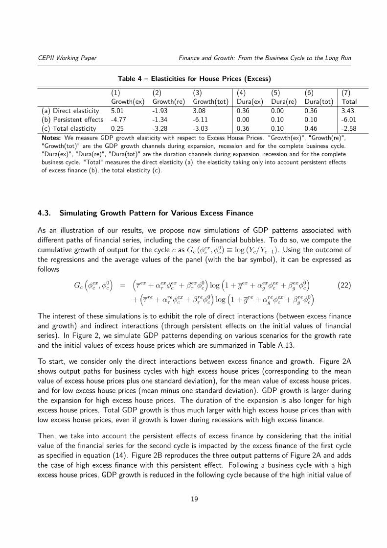
In Table 4, we measure GDP growth elasticity with respect to house prices (excess). Column (7)reports total elasticity as the sum of the growth channel (columns (1) to (3)) and the durationchannel (columns (4) to (6)) in three cases: (a) the direct effect where we only measure thecontemporaneous effect of excess finance, (b) taking into account only the persistent effect ofexcess finance, (c) the total effect.
For the direct effect (a), we estimate equation (13) of Section 2.2 that measures the elasticitybetween growth and excess finance for a complete business cycle. Concerning the growth channel,the total elasticity is equal to 3.08% (column (3)), a number that is the sum of the elasticitiesduring the expansion (that is 5.01%, column (1)) and the recession (that is −1.93%, column (2)).The value of π̄ex introduced in equation (13) for our panel is 0.745, that is economies are in averagethree quarters of the time in expansion and one quarter of the time in recession. This explainswhy the growth channel is positive even if the negative coefficient of excess finance for recessionsin Table 2 is larger in absolute value than the positive coefficient of excess finance for expansions.The gap between the growth channel and the total direct elasticity is explained by the durationchannel, which is equal to 0.36% (column (6)) and therefore accounts for almost 11% of the directelasticity. The duration channel is positive because excess finance is associated with longer durationof expansion and as the economic growth is in average higher in expansions than in recessions – thecorresponding rates are 2.19% and −0.11%.
We measure in line (b) of Table 4 the persistent effect of excess finance. We use equation (17) inSection 2.3. The elasticity is negative (−6.01%, column (7)), mainly because of a negative elasticityfor the growth channel. The elasticity for the growth channel is indeed equal to −6.11% (column(3)), a number that is the sum of the elasticities during the expansion (namely −4.877%, column(1)) and the recession (namely −1.34%, column (2)).
We then measure in line (c) of Table 4 the total elasticity between growth and excess finance. Toestimate this elasticity, we use equation (19) of Section 2.3. This total elasticity is the sum of thedirect elasticity (line (a)) and of the persistent effect of excess finance calculated in line (b). We finda negative total elasticity (−2.58%, column (7)). Interestingly, this negative effects mainly comesfrom a negative effect for the growth channel during the recession period ((−3.28%, column (2))).The growth-channel effect during the expansion is comparatively rather small ((0.25%, column (1))).The duration channel has a positive effect on the total elasticity ((0.46%, column (6))). It accountsfor almost 18% of the total elasticity.
We finally compute the threshold given in Section 2.4. It measures the initial level of financial seriesuntil which excess finance has a positive effect on growth. For house prices, the threshold is equal to40% of the average value of house prices in the sample (Table A.12). It means that a high value forexcess finance is accompanied by a high level of economic growth during a typical business cycle butcan be offset in the subsequent cycle given the persistent effect of excess finance. If the subsequentcycle starts with a low level of financial series, the total effect remains positive. For most economiesof our panel, the average value of the financial series is above this threshold suggesting that thetotal effect of excess finance on growth is negative.
18
CEPII Working Paper Finance and Growth: From the Business Cycle to the Long Run
(a) Direct elasticity 5.01 -1.93 3.08 0.36 0.00 0.36 3.43(b) Persistent effects -4.77 -1.34 -6.11 0.00 0.10 0.10 -6.01(c) Total elasticity 0.25 -3.28 -3.03 0.36 0.10 0.46 -2.58Notes: We measure GDP growth elasticity with respect to Excess House Prices. "Growth(ex)", "Growth(re)","Growth(tot)" are the GDP growth channels during expansion, recession and for the complete business cycle."Dura(ex)", "Dura(re)", "Dura(tot)" are the duration channels during expansion, recession and for the completebusiness cycle. "Total" measures the direct elasticity (a), the elasticity taking only into account persistent effectsof excess finance (b), the total elasticity (c).
4.3. Simulating Growth Pattern for Various Excess Finance
As an illustration of our results, we propose now simulations of GDP patterns associated withdifferent paths of financial series, including the case of financial bubbles. To do so, we compute thecumulative growth of output for the cycle c as Gc (φexc , φ0
c) ≡ log (Yc/Yc−1). Using the outcome ofthe regressions and the average values of the panel (with the bar symbol), it can be expressed asfollows
Gc
(φexc , φ
0c
)=
(τ ex + αexτ φ
exc + βexτ φ
0c
)log
(1 + gex + αexg φ
exc + βexg φ
0c
)(22)
+(τ re + αreτ φ
exc + βreτ φ
0c
)log
(1 + gre + αreg φ
exc + βreg φ
0c
)The interest of these simulations is to exhibit the role of direct interactions (between excess financeand growth) and indirect interactions (through persistent effects on the initial values of financialseries). In Figure 2, we simulate GDP patterns depending on various scenarios for the growth rateand the initial values of excess house prices which are summarized in Table A.13.
To start, we consider only the direct interactions between excess finance and growth. Figure 2Ashows output paths for business cycles with high excess house prices (corresponding to the meanvalue of excess house prices plus one standard deviation), for the mean value of excess house prices,and for low excess house prices (mean minus one standard deviation). GDP growth is larger duringthe expansion for high excess house prices. The duration of the expansion is also longer for highexcess house prices. Total GDP growth is thus much larger with high excess house prices than withlow excess house prices, even if growth is lower during recessions with high excess finance.
Then, we take into account the persistent effects of excess finance by considering that the initialvalue of the financial series for the second cycle is impacted by the excess finance of the first cycleas specified in equation (14). Figure 2B reproduces the three output patterns of Figure 2A and addsthe case of high excess finance with this persistent effect. Following a business cycle with a highexcess house prices, GDP growth is reduced in the following cycle because of the high initial value of
19
CEPII Working Paper Finance and Growth: From the Business Cycle to the Long Run
Figure 2 – SIMULATION OF OUTPUT PATHS FOR VARIATIONS IN EXCESS HOUSEPRICES
(C) Output Paths with Hysteresis and Bursting Bubble
Notes: Figure 2A shows output paths for business cycles with high excess house prices (cor-responding to the mean value of excess house prices plus one standard deviation ("M+1sd",in blue), for the mean value of excess house prices ("M", in black), and for low excess houseprices (mean minus one standard deviation, in red). Figure 2B reproduces the three outputpatterns of Figure 2A and adds the case of high excess finance with a persistent effect in cycle2 ("C2", Blue dash-line). Figure 2C shows the case of a first cycle ("C1") with a high excesshouse prices followed by a cycle with persistent effects on the initial values of house pricesand a low excess house prices (Mean minus one standard deviation, "M-1sd+persistence(C2)",Blue dash-line) – the three benchmark paths of the Figure 2A are also reproduced. We showcoefficients that are significantly different form zero at the 10% level, otherwise the zero valueis imposed.
CEPII Working Paper Finance and Growth: From the Business Cycle to the Long Run
house prices. The initial value of house prices (that is the value of house prices at the beginning ofeach business cycle) is indeed negatively correlated with GDP growth (Table 2). At the end of thefirst cycle, output is higher in the high excess finance case, but it is not necessary the case at theend of the subsequent cycles. Indeed, for this simulation, the solid blue lines overtakes the dottedblue line at the end of the period.
Finally we consider output paths in the case of a bursting bubble. Financial bubble is a very largeconcept to describe situations in which market prices diverge lastingly from their fundamental orequilibrium values in such a way that market corrections should occur to restore market equilibrium.In our data, financial growth is defined for financial series that try to capture such divergence, as theprice-to-rent ratio and credit-to-ouput. However, it is hard to distinguish in the data the fluctuationsof theses series that result from structural shifts of the economy from those that result from purelybubble/speculative behaviors. Nevertheless, our methodology can be informative to characterize thepattern of economic growth associated with a financial bubble. Once again, we do not measurehere the causal impact of a financial bubble on economic growth, but we identify the joint behaviorof economic and financial growth during business cycles. More precisely, we describe the patternof financial bubbles as exhibited in Table A.14, that is by the alternation of positive and negativevalues for excess finance – see for example the cases of France, Spain or the United Kingdom. Wepropose to simulate the consequences of a bubble defined as follows
φexc =
sd (φex)−δ × sd (φex)0
, if c = c̃, if c = c̃+ 1otherwise
(23)
where sd is the standard deviation of the financial series considered and δ is the size of the con-traction of the bubble. Figure 2C shows the case of a first cycle with a high excess house pricesfollowed by a cycle with persistent effects linked to the initial values of house prices and a low excesshouse prices (Mean minus one standard deviation) – the three benchmark paths of the Figure 2Aare also reproduced. This corresponds to a bursting bubble. GDP growth is much reduced in thiscase because of the combination in the second cycle of low house prices growth and a high initialvalue of house prices. In Figure 2C, we consider δ = 1. In practice, we can observe situation wherethere is no full deleveraging (δ < 1). This situation is close to numerous examples of growth duringand after financial bubbles (as recently observed in Spain, see Table A.14). The interest of ourmethodology is to generate such patterns using estimates of growth-finance interactions throughthe growth and duration channels as well as the persistent effects of financial growth.
5. Robustness Checks
We propose robustness checks of the main results of the paper. We show that our regression resultsare roughly the same for other measures of excess finance. We show that our results are robustto controlling for endogeneity as recently suggested by Arcand et al. (2015). We control also our
21
CEPII Working Paper Finance and Growth: From the Business Cycle to the Long Run
results for properties of the financial cycle and for the occurrence of bank crisis. We finally test thehypothesis that the hysteresis effect could come from the link between finance and productivity.
5.1. Alternative measures of finance
We choose as the main specification house price excess. As robustness checks, we use five othermeasures of excess finance growth such as price-to-rent ratios, real credit, credit to GDP, realhouseholds credit, households credit to GDP.
Regression results for five alternative measures. The correlation between excess finance andGDP growth is very robust in expansion and recession for the five alternative measures. Price-to-rent ratios (excess), real credit (excess), credit to GDP (excess), real households credit (excess),households credit to GDP (excess) are all associated with higher GDP growth during the expansionand lower growth during the recession (columns (1) and (2) of Tables A.4, A.5, A.6, A.7, A.8).In contrast, the coefficients of correlation between economic growth and the initial values of allthese financial series are robustly negative and significantly different from zero both for expansionsand recessions. Concerning duration, the five different measures of excess finance growth indicatea strongly positive and significant correlation between excess finance growth and the duration ofthe expansion phase (columns (3) of Tables A.4, A.5, A.6, A.7, A.8). We find also a positive andsignificant correlation between excess finance growth and the duration of the recession in the caseof credit to GDP (column (9) of Table A.6).
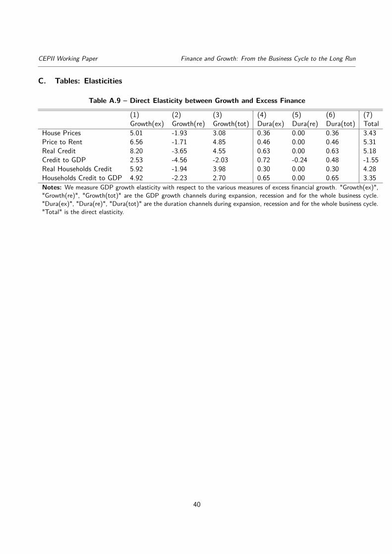
Elasticities for five other measures. In Table A.9, we report the direct elasticities for to thesix measures of excess finance. Column (7) reports the elasticity as the sum of the growth channel(columns (1) to (3)) and the duration channel (columns (4) to (5)). For five out of the six measuresof excess finance, the direct elasticity is positive. This is the case for house prices, price-to-rentratio, real credit, real households credit and households credit to GDP (the only exception is theratio of credit to GDP). When the persistent effect of excess finance is considered, in Table A.10,the elasticity is negative for all series considered with a range of values between −5.31 (for theReal Credit series) and −9.35 (for the ratio of household credit to GDP). Given these figures, thepersistent effect clearly outweighs the direct effect making the total effect negative for all series,see Table A.11. We compute also the threshold φ̂0 for each financial indicator in Table A.12. Inaverage for our six measures of excess finance, this threshold corresponds to a third of the level ofthe financial series observed in our sample in 2014-2015 or to 50% of the average level of financialseries. The fact that the average level of the financial series is well above this threshold explains thenegative elasticity between finance and growth we compute in Table A.11.
22
CEPII Working Paper Finance and Growth: From the Business Cycle to the Long Run
5.2. Endogeneity
Regressions in Section 4.1 show significant correlation between excess finance and growth even ifwe control for country fixed-effects and other determinants of economic growth as originally doneby King and Levine (1993). However, as emphasized by Beck (2009), OLS estimators may not beconsistent because of the omitted variable bias, the reverse causation from growth to excess finance,and measurement issues of variables. Instrumental Variables (IV) have been extensively used inthe growth-finance literature to overcome the biases of OLS estimators notably by instrumentingfinancial depth with legal origin in cross-country analysis (Levine (1998), Levine (1999)) or by usinglagged variables as internal instruments in dynamic panel analysis (Beck et al. (2000)). We followthe strategy recently proposed by Arcand et al. (2015) who use an identification strategy basedon the presence of heteroskedasticity in the regression’s residual. The interest of this methodologyoriginally developed by Rigobon (2003) and Lewbel (2012) is to improve the identification of causalrelationships even in the absence of external instruments16 - see Appendix B for details on theidentification strategy. Table 5 reports the estimates of the models of Tables 2 (columns (4), (5),and (6)) using identification through heteroskedasticity (Rigobon (2003), Lewbel (2012))17. As inthe OLS estimations of Table 2, we find a positive relationship between House Prices (Excess) andGDP growth during the expansion (column (1)) and a negative one during the recession (column(2)). The coefficients associated with House Prices (Excess) are precisely estimated, suggesting thatcov (X, ε2
2) is not close to zero and the Hansen’s J test fails to reject the overidentifying restrictionsat the 5% confidence level.
5.3. Controlling for the Financial Cycle and for Banking Crises
We control our results more precisely for the Financial cycle and for the occurrence of BankingCrises.
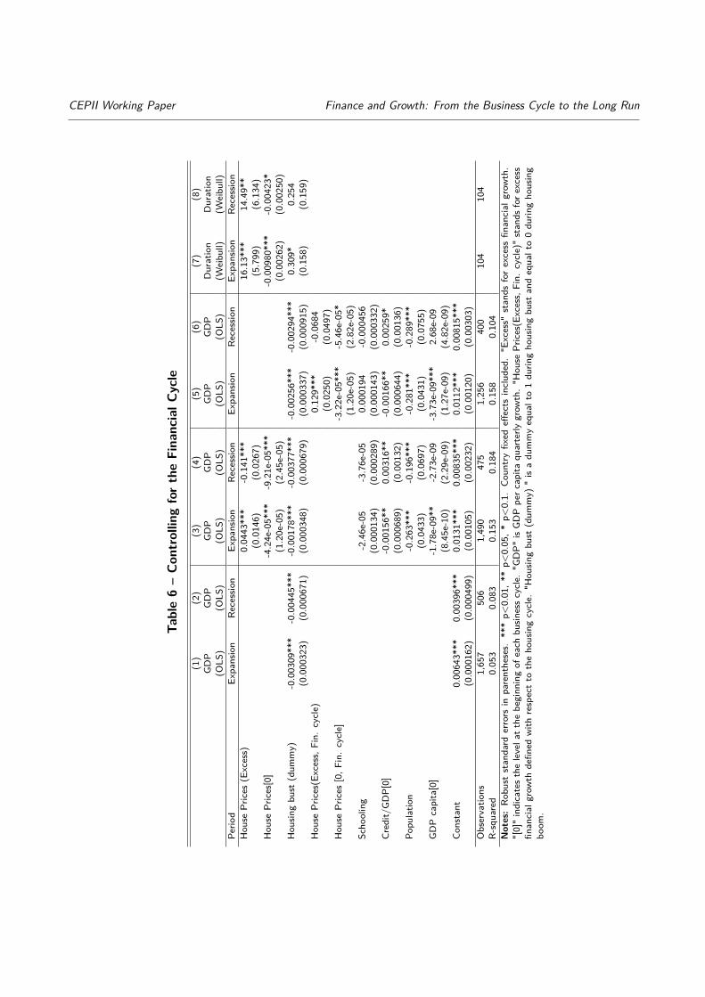
Controlling for the Financial Cycle. In our benchmark regressions, we consider the value offinancial series without taking into account the cycle of these series. In Table 6, we show that ourresults are robust controlling more precisely for the financial cycle. To define the financial cycle,we apply the algorithm of Harding and Pagan (2002) to identify local maxima (peaks) and minima(troughs) in the log-levels of real house prices in each country of our panel18. A financial cycle iscomposed of two phases: the financial boom phase starts after a trough and ends at the peak whichinitiates the financial bust phases up to the next trough. We create a financial bust dummy, equalto 1 during a financial bust and to 0 during a financial boom.16 As explained by Beck (2009), the challenge with external instruments "is to identify the economic mechanismsthrough which the instrumental variables influence the endogenous variable – financial activity – while at the sametime assuring that the instruments are not correlated with growth directly."17 We cannot use the same methodology for the Weibull regression model we use in Table 3. In this section, we thuschoose to focus on controlling the endogeneity of the OLS regressions.18We define the financial cycle using real house prices as this variable is the main specification in our paper.
23
CEPII Working Paper Finance and Growth: From the Business Cycle to the Long Run
(2.64e-10) (4.32e-10) (2.42e-10)Observations 1,909 514 2,423Hansen J Stat. 2.849 6.145 0.404p-value 0.583 0.189 0.982Notes: Robust standard errors in parentheses. *** p<0.01, ** p<0.05,* p<0.1. Country fixed effects included. "Excess" stands for excess fi-nancial growth. "[0]" indicates the level at the beginning of each businesscycle. "GDP growth" is GDP per capita quarterly growth. The causaleffect of House Prices (Excess) is identified using identification through het-eroskedasticity (Lewbel (2012)).
CEPII Working Paper Finance and Growth: From the Business Cycle to the Long Run
In columns (1) and (2) of the Table 6, we first verify that financial busts are indeed negativelycorrelated with GDP growth. As expected, this is the case both during business cycle expansions(column (1)) and recessions (columns (2)). We then show that our main results described in Table 2are robust controlling for the financial cycle: excess finance is positively correlated with GDP duringthe expansion (column (3)) and negatively correlated during the recession (column (4)). As in Table2, the coefficient of the initial value of the financial series is also negative for the two business cyclephases, the expansion and recession. The duration regressions are also robust controlling for thefinancial cycle (see Table 3). In particular, large excess house prices are associated with a longerduration of expansions (column (7)).
Finally, instead of using our standard measure of excess finance (defined from a business cycle troughto a business cycle peak), we define excess finance specifically for the financial boom period (thatis, from a financial cycle trough to the financial cycle peak). Excess finance is positively correlatedwith GDP growth during the business cycle expansion (column (5)), and negatively correlated duringthe recession (column (6)). The coefficient during the recession is however weakly significant (17%level). We define also the initial value of the financial series with respect to the financial cycle: aspreviously, we find a negative correlation with GDP growth both during the expansion (column (5))and the recession (column (6)).
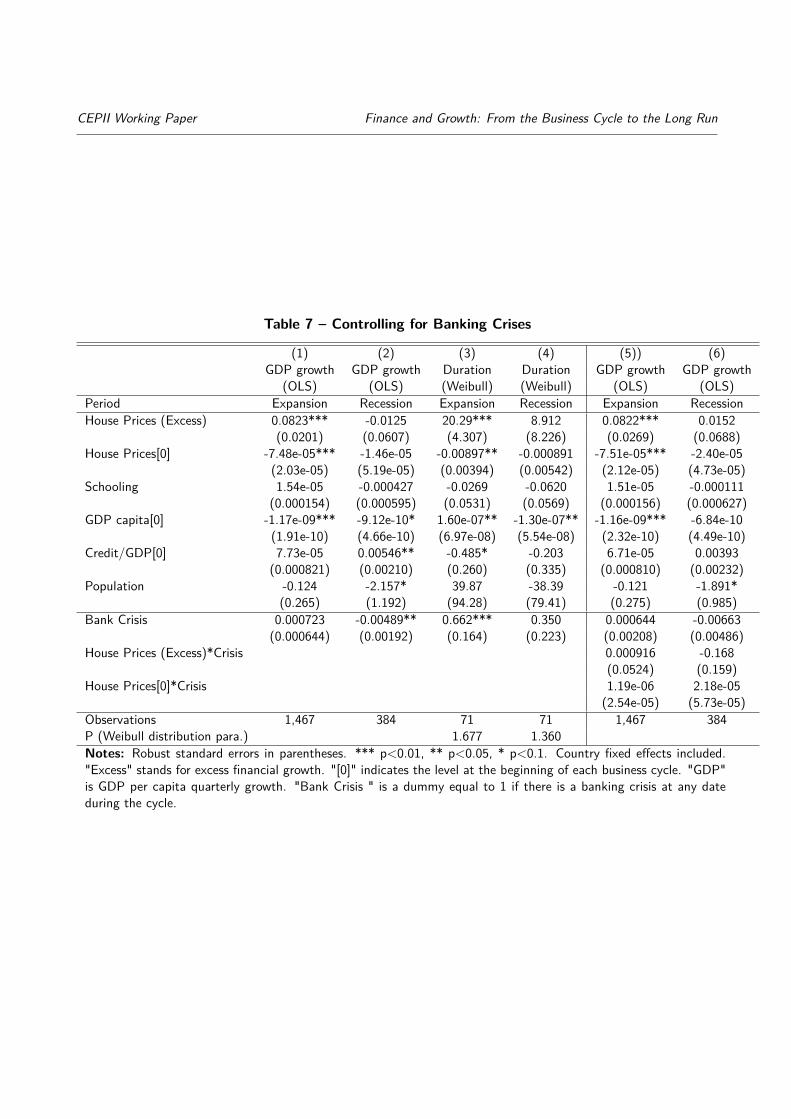
Financial crises Banking crises could be the culprits that lie behind the persistent effect of excessfinance. In table 7, we test this prediction. We first show that the main results of the paper arerobust controlling for a Banking crisis dummy. In particular, during expansion periods, excess houseprices are positively correlated with GDP growth (column (1)) and to the duration of expansion(column (3)). The initial level of house prices is negatively correlated both with GDP growth andwith the duration of expansion. These two variables are not correlated during recessions (columns(2) and (4)). We find the same results when adding interaction terms between Excess House Pricesand the banking crisis dummy or between House Prices [0] and the banking crisis dummy. Thesetwo interaction terms are not significant (columns (5) and (6)). These results seem to indicate thatbanking crises do no explain the persistent effect of excess finance. Similarly, our results do notseem specific to bank crisis periods.
25
CEPII Working Paper Finance and Growth: From the Business Cycle to the Long Run
Table6–Con
trollingfortheFinancialC
ycle
(1)
(2)
(3)
(4)
(5)
(6)
(7)
(8)
GDP
GDP
GDP
GDP
GDP
GDP
Duration
Duration
(OLS
)(O
LS)
(OLS
)(O
LS)
(OLS
)(O
LS)
(Weibu
ll)(W
eibu
ll)Pe
riod
Expansion
Recession
Expansion
Recession
Expansion
Recession
Expansion
Recession
Hou
sePrices
(Excess)
0.0443***
-0.141***
16.13***
14.49**
(0.0146)
(0.0267)
(5.799)
(6.134)
Hou
sePrices[0]
-4.24e-05***
-9.21e-05***
-0.00980***
-0.00423*
(1.20e-05)
(2.45e-05)
(0.00262)
(0.00250)
Hou
singbu
st(dum
my)
-0.00309***
-0.00445***
-0.00178***
-0.00377***
-0.00256***
-0.00294***
0.309*
0.254
(0.000323)
(0.000671)
(0.000348)
(0.000679)
(0.000337)
(0.000915)
(0.158)
(0.159)
Hou
sePrices(Excess,Fin.
cycle)
0.129***
-0.0684
(0.0250)
(0.0497)
Hou
sePrices
[0,F
in.cycle]
-3.22e-05***
-5.46e-05*
(1.20e-05)
(2.82e-05)
Scho
oling
-2.46e-05
-3.76e-05
0.000194
-0.000456
(0.000134)
(0.000289)
(0.000143)
(0.000332)
Credit/
GDP[0]
-0.00156**
0.00316**
-0.00166**
0.00259*
(0.000689)
(0.00132)
(0.000644)
(0.00136)
Popu
latio
n-0.263***
-0.196***
-0.281***
-0.289***
(0.0433)
(0.0697)
(0.0431)
(0.0755)
GDPcapita[0]
-1.78e-09**
-2.73e-09
-3.73e-09***
2.68e-09
(8.45e-10)
(2.29e-09)
(1.27e-09)
(4.82e-09)
Constant
0.00643***
0.00396***
0.0131***
0.00835***
0.0112***
0.00815***
(0.000162)
(0.000499)
(0.00105)
(0.00232)
(0.00120)
(0.00303)
Observatio
ns1,657
506
1,490
475
1,256
400
104
104
R-squared
0.053
0.083
0.153
0.184
0.158
0.104
Notes:Ro
bust
standard
errors
inparentheses.
***p<
0.01,**
p<0.05,*p<
0.1.
Coun
tryfixed
effects
includ
ed."E
xcess"
stands
forexcess
financial
grow
th.
"[0]"indicatesthelevela
tthebeginn
ingof
each
busin
esscycle.
"GDP"
isGDPperc
apita
quarterly
grow
th."H
ouse
Prices(Excess,Fin.
cycle)"stands
fore
xcess
financial
grow
thdefin
edwith
respectto
theho
usingcycle.
"Hou
singbu
st(dum
my)
"isadu
mmyequalto1du
ringho
usingbu
standequalto0du
ringho
using
boom
.
CEPII Working Paper Finance and Growth: From the Business Cycle to the Long Run
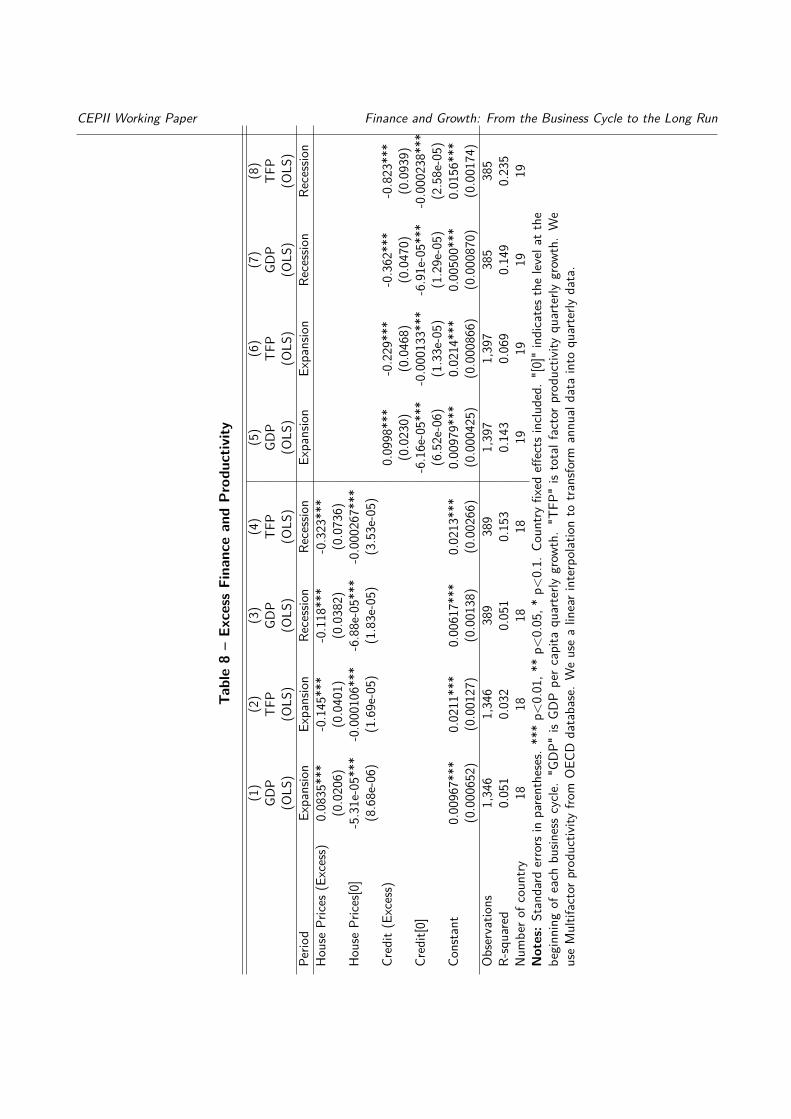
5.4. Finance and productivity
The link between finance and productivity could be an explanation of the hysteresis effect of excessfinance. According to Cecchetti and Kharroubi (2015) and Borio et al. (2016), credit booms tend toundermine productivity growth by inducing labour reallocations towards lower productivity growthsectors, in particular the construction sector. The financial sector’s expansion may indeed benefitdisproportionately to projects with high collateral but low productivity. This could explain thenegative effect of the excessive development of finance inherited from previous cycles. Testingfully this hypothesis is beyond the scope of this paper. However, we show in Table 8 that duringexpansions, if excess finance is positively correlated with GDP growth (columns (1) and (5) for Houseprices (excess) and Credit (excess)), it is negatively correlated with total factor productivity (TFP)growth (columns (2) and (6)). The initial level of financial activity is also negatively correlated withTFP growth. We show also that during recessions, excess finance is negatively correlated with TFPgrowth (columns (4) and (8)). These results could suggest that financial booms affect negativelyproductivity with long-term consequences on GDP growth.
27
CEPII Working Paper Finance and Growth: From the Business Cycle to the Long Run
Table 7 – Controlling for Banking Crises
(1) (2) (3) (4) (5)) (6)GDP growth GDP growth Duration Duration GDP growth GDP growth
(2.54e-05) (5.73e-05)Observations 1,467 384 71 71 1,467 384P (Weibull distribution para.) 1.677 1.360Notes: Robust standard errors in parentheses. *** p<0.01, ** p<0.05, * p<0.1. Country fixed effects included."Excess" stands for excess financial growth. "[0]" indicates the level at the beginning of each business cycle. "GDP"is GDP per capita quarterly growth. "Bank Crisis " is a dummy equal to 1 if there is a banking crisis at any dateduring the cycle.
CEPII Working Paper Finance and Growth: From the Business Cycle to the Long Run
Table8–Ex
cess
FinanceandProdu
ctivity
(1)
(2)
(3)
(4)
(5)
(6)
(7)
(8)
GDP
TFP
GDP
TFP
GDP
TFP
GDP
TFP
(OLS
)(O
LS)
(OLS
)(O
LS)
(OLS
)(O
LS)
(OLS
)(O
LS)
Perio
dEx
pansion
Expansion
Recession
Recession
Expansion
Expansion
Recession
Recession
Hou
sePrice
s(Excess)
0.0835***
-0.145***
-0.118***
-0.323
***
(0.0206)
(0.0401)
(0.0382)
(0.0736)
Hou
sePrice
s[0]
-5.31e-05***
-0.000106***
-6.88e-05***
-0.000267*
**(8.68e-06)
(1.69e-05)
(1.83e-05)
(3.53e-05)
Credit(Excess)
0.0998***
-0.229***
-0.362***
-0.823***
(0.0230)
(0.0468)
(0.0470)
(0.0939)
Credit[0]
-6.16e-05***
-0.000133***
-6.91e-05***
-0.000238***
(6.52e-06)
(1.33e-05)
(1.29e-05)
(2.58e-05)
Constant
0.00967***
0.0211***
0.00617***
0.0213***
0.00979***
0.0214***
0.00500***
0.0156***
(0.000652)
(0.00127)
(0.00138)
(0.00266)
(0.000425)
(0.000866)
(0.000870)
(0.00174)
Observatio
ns1,346
1,346
389
389
1,397
1,397
385
385
R-squared
0.051
0.032
0.051
0.153
0.143
0.069
0.149
0.235
Num
bero
fcou
ntry
1818
1818
1919
1919
Notes:Standard
errors
inparentheses.
***p<
0.01,*
*p<
0.05,*
p<0.1.
Coun
tryfixed
effects
inclu
ded.
"[0]"indicatesthelev
elat
the
beginn
ingof
each
busin
esscycle
."G
DP"
isGD
Ppercapita
quarterly
grow
th."T
FP"istotalfactorprod
uctiv
ityqu
arterly
grow
th.We
useMultifactorp
rodu
ctivity
from
OEC
Ddatabase.Weusealinearinterpo
latio
nto
transfo
rmannu
aldata
into
quarterly
data.
CEPII Working Paper Finance and Growth: From the Business Cycle to the Long Run
6. Concluding Remarks
We propose in this paper a new methodology to study the interactions between excess financialgrowth and economic growth. We show that the finance-growth elasticity in the long-run can beviewed as the cumulative of finance-growth interactions within each cycle through a growth channeland a duration channel. Our empirical analysis delivers two key properties of the interactions betweenfinance and growth.
We first show that the contemporaneous elasticity between financial and economic growth rates ispositive, even if high financial growth makes recessions more severe. It is in line with Jordà et al.(2013) who show that credit-intensive expansions tend to be followed by deeper recessions. It is alsocoherent with Loayza and Ranciere (2006) who find a positive long-run relationship between financialintermediation and output growth that co-exists with a mostly negative short-run relationship. Inour paper, growth supplements result not only from higher average growth rate but also from longerduration of expansions. The identification of a link between finance and expansion duration is anew contribution to the literature. In our paper, high excess finance is accompanied by a longerduration of expansions. The duration channel accounts for one fifth of total elasticity in the case ofhouse prices. Several mechanisms could explain this property. A first interpretation could be basedon the procyclical behaviour of finance as stated by the financial accelerator mechanism developedby Bernanke et al. (1999). Indeed, an improvement of the fundamentals of the economic leads tomore both growth and financial activities. A second interpretation could be based on the "time isdifferent" syndrome developed by Reinhart and Rogoff (2008). A long expansion may be a favorablecontext for the development of beliefs at the origin of excessive developments of financial activities.A third interpretation could be that bubbles in the expansion phase can play as a shock absorber.An oil shock could be for example more easily absorbed in a country when growth is fed by a bubble.Further research would be needed to investigate the links between the duration of expansion andexcess finance, in particular the sense of causality and economic mechanisms behind the relationship.
Beyond the contemporaneous effects of financial booms, we show that the elasticity between fi-nancial and economic growth turns out negative when the persistent effects of excess finance aretaken into account. More precisely, financial and economic growth rates are positively correlatedonly up to a certain threshold of financial activity. As the average level of financial activity is wellabove this threshold, we get a negative total elasticity between finance and growth. This secondproperty can be related to the concept of "Debt Supercycle" developed by Rogoff (2015) accordingto which the inheritance of excessive development of finance in the past can lead to long-lastinglow economic growth. This result could also be linked to the notion of deleveraging crisis formal-ized by Eggertsson and Krugman (2012). Another potential explanation is based on the long-runconsequences of financial booms on productivity. Evidence described in this paper seem to suggestthat excess finance is positively correlated with GDP growth but negatively correlated with totalfactor productivity (TFP) growth. This could be explained by the mechanism described by Borioet al. (2016) according to which credit booms tend to undermine productivity growth by inducinglabour reallocations towards lower productivity growth sectors. More research would be needed to
30
CEPII Working Paper Finance and Growth: From the Business Cycle to the Long Run
investigate the hysteresis effect and the consequences of financial booms on productivity.
31
CEPII Working Paper Finance and Growth: From the Business Cycle to the Long Run
References
Arcand, J.-L., Berkes, E., and Panizza, U. (2015). Too much finance? Journal of Economic Growth,Volume 20(Issue 2).
Beck, T. (2009). The econometrics of finance and growth. Springer.Beck, T., Demirgüç-Kunt, A., and Levine, R. (2007). Finance, inequality and the poor. Journal of
economic growth, 12(1):27–49.Beck, T., Levine, R., and Loayza, N. (2000). Finance and the sources of growth. Journal of Financial
Economics, 58:261–300.Benhabib, J. and Spiegel, M. M. (2000). The role of financial development in growth and investment.
Journal of economic growth, 5(4):341–360.Bernanke, B. S., Gertler, M., and Gilchrist, S. (1999). The financial accelerator in a quantitative
business cycle framework. Handbook of macroeconomics, 1:1341–1393.Blanchard, O., Cerutti, E., and Summers, L. (2015). Inflation and Activity Two Explorations and
their Monetary Policy Implications. Working Paper 21726, National Bureau of Economic Research.Bonfiglioli, A. (2008). Financial integration, productivity and capital accumulation. Journal of
International Economics, 76(2):337–355.Borio, C., Disyatat, P., and Juselius, M. (2013). Rethinking potential output : Embedding informa-
tion about the financial cycle. Bank for International Settlements.Borio, C. E., Kharroubi, E., Upper, C., and Zampolli, F. (2016). Labour reallocation and productivity
dynamics: financial causes, real consequences.Bry, G. and Boschan, C. (1971). Programmed selection of cyclical turning points. In Cyclical
Analysis of Time Series: Selected Procedures and Computer Programs, pages 7–63. NBER.Cecchetti, S. G. and Kharroubi, E. (2012). Reassessing the impact of finance on growth. BIS
Working Paper, (381).Cecchetti, S. G. and Kharroubi, E. (2015). Why does financial sector growth crowd out real economic
growth?Claessens, S., Kose, M. A., and Terrones, M. E. (2012). How do business and financial cycles
interact? Journal of International Economics, 87(1):178–190.Diebold, F. X., Rudebusch, G., and Sichel, D. (1993). Further evidence on business-cycle duration
dependence. In Business cycles, indicators and forecasting, pages 255–284. University of ChicagoPress.
Drehmann, M., Borio, C. E. V., and Tsatsaronis, K. (2012). Characterising the financial cycle: don’tlose sight of the medium term! BIS Working Paper 380.
Eggertsson, G. B. and Krugman, P. (2012). Debt, deleveraging, and the liquidity trap: A fisher-minsky-koo approach*. The Quarterly Journal of Economics, 127:1469—-1513.
Gadea Rivas, M. D. and Perez-Quiros, G. (2015). the Failure To Predict the Great Recession-a ViewThrough the Role of Credit. Journal of the European Economic Association, 13(3):534–559.
32
CEPII Working Paper Finance and Growth: From the Business Cycle to the Long Run
Gali, J. (2016). Insider-outsider labor markets, hysteresis and monetary policy. Economics WorkingPapers 1506, Department of Economics and Business, Universitat Pompeu Fabra.
Goldsmith, R. (1969). Financial structure and economic development. Yale University Press.Harding, D. and Pagan, A. (2002). Dissecting the cycle: a methodological investigation. Journal of
monetary economics, 49(2):365–381.Jenkins, S. P. (2005). Survival analysis. Unpublished manuscript, Institute for Social and Economic
Research, University of Essex, Colchester, UK.Jordà, Ò., Schularick, M., and Taylor, A. M. (2013). When Credit Bites Back. Journal of Money,
Credit and Banking, 45(s2):3–28.Jordà, Ò., Schularick, M., and Taylor, A. M. (2016). The great mortgaging: Housing finance, crises,
and business cycles. Economic Policy, 31:107—-152.King, R. G. and Levine, R. (1993). Finance and growth: Schumpeter might be right. The Quarterly
Journal of Economics, 108(3):717–737.Krugman, P. (2013). Secular Stagnation, Coalmines, Bubbles, and Larry Summers. New York
Times, (November 16), pages 1–6.Levine, R. (1997). Economic Development and Financial and Agenda Growth: Views and Agenda.
Journal of Economic Literature, 35(2):688–726.Levine, R. (1998). The legal environment, banks, and long-run economic growth. Journal of money,
credit and banking, pages 596—-613.Levine, R. (1999). Law, finance, and economic growth. Journal of financial Intermediation, 8(1):8–
35.Lewbel, A. (2012). Using heteroscedasticity to identify and estimate mismeasured and endogenous
regressor models. Journal of Business & Economic Statistics, 30(1):67–80.Lo, S. H. and Rogoff, K. (2015). Secular stagnation, debt overhang and other rationales for sluggish
growth, six years on. BIS Working Paper 482.Loayza, N. V. and Ranciere, R. (2006). Financial development, financial fragility, and growth.
Journal of Money, Credit and Banking, pages 1051–1076.McKinnon, R. I. (1973). Money and capital in economic development. Brookings Institution Press.Mian, A. R., Sufi, A., and Verner, E. (2015). Household debt and business cycles worldwide. Working
Paper 21581, National Bureau of Economic Research.Pesaran, M. H., Shin, Y., and Smith, R. P. (1999). Pooled mean group estimation of dynamic
heterogeneous panels. Journal of the American Statistical Association, 94(446):621–634.Rancière, R. and Tornell, A. (2016). Financial Liberalization, Debt Mismatch, Allocative Efficiency
and Growth. American Economic Journal: Macroeconomics, 8:1—-44.Ranciere, R., Tornell, A., and Westermann, F. (2006). Decomposing the effects of financial liberal-
ization: Crises vs. growth. Journal of Banking and Finance, 30(12):3331–3348.Reinhart, C. M. and Rogoff, K. (2008). This time is different: Eight centuries of financial folly.
33
CEPII Working Paper Finance and Growth: From the Business Cycle to the Long Run
Princeton Univ Press.Rigobon, R. (2003). Identification through heteroskedasticity. Review of Economics and Statistics,
85(4):777–792.Rogoff, K. (2015). Debt supercycle, not secular stagnation. Vox: CEPR Policy Portal.Rousseau, P. L. and Wachtel, P. (2011). What is happening to the impact of financial deepening
on economic growth? Economic Inquiry, 49(1):276–288.Rousseau, P. L. and Wachtel, P. (2015). Episodes of Financial Deepening: Credit Booms or Growth
Generators? (March):1–27.Schularick, M. and Taylor, A. M. (2012). Credit Booms Gone Bust: Monetary Policy, Leverage
Cycles, and Financial Crises, 1870-2008. The American Economic Review, 102(2):1029–1061.Sichel, D. E. (1991). Business cycle duration dependence: A parametric approach. The Review of
Economics and Statistics, pages 254–260.Stock, J. H. and Watson, M. W. (1999). Business cycle fluctuations in us macroeconomic time
series. 1:3–64.Summers, L. (2013). Why stagnation might prove to be the new normal. The Financial Times,
December 1.Summers, L. H. (2015). Reflections on Secular Stagnation.Terrones, M. E., Scott, A., Kannan, P., and Others (2009). From recession to recovery: How soon
and how strong? International Monetary Fund, World Economic Outlook, April.
34
CEPII Working Paper Finance and Growth: From the Business Cycle to the Long Run
Appendix
A. Tables
A. Tables: Summary Statistics and Variables definitions
(0.000611) (0.00113)Observations 2,200 756 160 160Number of countries 24 24 24 24R2 0.040 0.037P (Weibull distribution para.) 1.264 1.343Notes: Standard errors in parentheses. *** p<0.01, ** p<0.05, * p<0.1. Country fixedeffects included. "Excess" stands for excess financial growth. "[0]" indicates the level atthe beginning of each business cycle. "GDP growth" is real GDPquarterly growth percapita. "Duration" stands for the duration (in quarters) of each phase of the businesscycle.
37
CEPII Working Paper Finance and Growth: From the Business Cycle to the Long Run
Table A.5 – Real Credit
(1) (2) (3) (4)GDP growth GDP growth Duration Duration
(0.000240) (0.000451)Observations 2,794 842 180 180Number of countries 24 24 24 24R2 0.103 0.048P (Weibull distribution para.) 1.330 1.300Notes: Standard errors in parentheses. *** p<0.01, ** p<0.05, * p<0.1. Country fixedeffects included. "Excess" stands for excess financial growth. "[0]" indicates the level atthe beginning of each business cycle. "GDP growth" is real GDPquarterly growth percapita. "Duration" stands for the duration (in quarters) of each phase of the businesscycle.
Table A.6 – Credit/GDP
(1) (2) (3) (4)GDP growth GDP growth Duration Duration
(0.000397) (0.000706)Observations 2,828 868 186 186Number of countries 24 24 24 24R2 0.062 0.058P (Weibull distribution para.) 1.301 1.306Notes: Standard errors in parentheses. *** p<0.01, ** p<0.05, * p<0.1. Country fixedeffects included. "Excess" stands for excess financial growth. "[0]" indicates the level atthe beginning of each business cycle. "GDP growth" is real GDPquarterly growth percapita. "Duration" stands for the duration (in quarters) of each phase of the businesscycle.
CEPII Working Paper Finance and Growth: From the Business Cycle to the Long Run
Table A.7 – Real Households Credit
(1) (2) (3) (4)GDP growth GDP growth Duration Duration
(0.000287) (0.000557)Observations 1,973 545 117 117Number of countries 22 22 22 22R2 0.139 0.020P (Weibull distribution para.) 1.364 1.459Notes: Standard errors in parentheses. *** p<0.01, ** p<0.05, * p<0.1. Country fixedeffects included. "Excess" stands for excess financial growth. "[0]" indicates the level atthe beginning of each business cycle. "GDP growth" is real GDP quarterly growth percapita. "Duration" stands for the duration (in quarters) of each phase of the businesscycle.
Table A.8 – Households Credit/GDP
(1) (2) (3) (4)GDP growth GDP growth Duration Duration
(0.000443) (0.000787)Observations 1,973 545 117 117Number of countries 22 22 22 22R2 0.104 0.020P (Weibull distribution para.) 1.325 1.460Notes: Standard errors in parentheses. *** p<0.01, ** p<0.05, * p<0.1. Country fixedeffects included. "Excess" stands for excess financial growth. "[0]" indicates the level atthe beginning of each business cycle. "GDP growth" is real GDP quarterly growth percapita. "Duration" stands for the duration (in quarters) of each phase of the businesscycle.
CEPII Working Paper Finance and Growth: From the Business Cycle to the Long Run
C. Tables: Elasticities
Table A.9 – Direct Elasticity between Growth and Excess Finance
House Prices 5.01 -1.93 3.08 0.36 0.00 0.36 3.43Price to Rent 6.56 -1.71 4.85 0.46 0.00 0.46 5.31Real Credit 8.20 -3.65 4.55 0.63 0.00 0.63 5.18Credit to GDP 2.53 -4.56 -2.03 0.72 -0.24 0.48 -1.55Real Households Credit 5.92 -1.94 3.98 0.30 0.00 0.30 4.28Households Credit to GDP 4.92 -2.23 2.70 0.65 0.00 0.65 3.35Notes: We measure GDP growth elasticity with respect to the various measures of excess financial growth. "Growth(ex)","Growth(re)", "Growth(tot)" are the GDP growth channels during expansion, recession and for the whole business cycle."Dura(ex)", "Dura(re)", "Dura(tot)" are the duration channels during expansion, recession and for the whole business cycle."Total" is the direct elasticity.
40
CEPII Working Paper Finance and Growth: From the Business Cycle to the Long Run
Table A.10 – Elasticity when measuring the Persistent Effects of Excess Finance
House Prices -4.77 -1.34 -6.11 0.00 0.10 0.10 -6.01Prices to Rent -3.36 -2.14 -5.50 0.00 0.00 0.00 -5.50Real Credit -4.07 -1.24 -5.31 0.00 0.00 0.00 -5.31Credit to GDP -6.41 -1.58 -7.99 0.00 0.00 0.00 -7.99Real Households Credit -5.15 -0.78 -5.93 -0.14 0.00 -0.14 -6.07Households Credit to GDP -8.47 -0.87 -9.35 0.00 0.00 0.00 -9.35Notes: We measure GDP growth elasticity with respect to the various measures of excess financial growth. "Growth(ex)","Growth(re)", "Growth(tot)" are the GDP growth channels during expansion, recession and in the long-run measuring onlythe persistent effects of Excess finance. "Dura(ex)", "Dura(re)", "Dura(tot)" are the duration channels during expansion,recession and in the long-run measuring only the persistent effects of Excess finance. "Total" is the long-run elasticitymeasuring only the persistent effects of Excess finance.
Table A.11 – Total Elasticity between Growth and Excess Finance with Hysteresis
House Prices 0.25 -3.28 -3.03 0.36 0.10 0.46 -2.58Price to Rent 3.20 -3.85 -0.65 0.46 0.00 0.46 -0.19Real Credit 4.12 -4.89 -0.77 0.63 0.00 0.63 -0.13Credit to GDP -3.87 -6.14 -10.02 0.72 -0.24 0.48 -9.54Households Credit 0.78 -2.72 -1.95 0.17 0.00 0.17 -1.78Households Credit to GDP -3.55 -3.10 -6.65 0.65 0.00 0.65 -6.00Notes: We measure GDP growth elasticity with respect to the various measures of excess financial growth. "Growth(ex)","Growth(re)", "Growth(tot)" are the GDP growth channels during expansion, recession and in the long-run. "Dura(ex)","Dura(re)", "Dura(tot)" are the duration channels during expansion, recession and in the long-run. "Total" is the totallong-run elasticity.
Table A.12 – Threshold for the initial value of Financial series
(1) (2) (3)Threshold Mean Value %
House Prices 36.07 75.85 41%Price to Rent 58.39 82.10 71%Real Credit 35.89 59.15 61%Credit to GDP . . .Households Credit 29.68 65.15 46%Households Credit to GDP 0.13 0.50 26%Notes: All series (except Households Credit to GDP) are indices (base100=2005). In column 1, the threshold is equal to 36% of house pricevalue in 2005. We cannot measure a threshold for credit to GDP as in thiscase the direct effect is negative. Column (2) indicates the mean value ofthe initial level of the financial series. We divide in column (3) the value ofthe threshold (column (1)) by the mean value (column (2)).
CEPII Working Paper Finance and Growth: From the Business Cycle to the Long Run
D. Tables for Simulations and Figure 2
Table A.13 – Business Cyclesc = 1 c = 2 c = 3
The Mean Case φexc 0 0 0Panels A, B, C (black lines) φ0
c φ0
φ0
φ0
The Low Excess Finance Case φexc −sd (φex) −sd (φex) −sd (φex)Panels A, B, C (dotted red lines) φ0
c φ0
φ0
φ0
The High Excess Finance Case φexc sd (φex) sd (φex) sd (φex)Panel A (blue line) φ0
c φ0
φ0
φ0
... with persistence φexc sd (φex) 0 0Panel B (dashed blue line) φ0
c φ0
φ0 + φex1 τex1 φ0
2... with bubbles φexc sd (φex) −δ × sd (φex) 0Panel C (dashed blue line) φ0
c φ0
φ0 + φex1 τex1 φ0
1 + φex2 τex2
Table A.14 – House Prices (Excess) and House Prices[0]: Descriptive Statistics for the twolast complete business cycles
Cycle 2 2002q1 2007q4 .0022039 81.79Notes: We use house prices as a measure for Excess Finance and "Finance Init"(the level of House Prices at the beginning of each business cycle). We consideronly the two last and complete business cycles in each country.
42
CEPII Working Paper Finance and Growth: From the Business Cycle to the Long Run
B. Identification Strategy
To explain the identification strategy, we follow the exposition of Lewbel (2012) and its applicationin the finance-growth literature by Arcand et al. (2015). Let Y1 and Y2 be observed endogenousvariables, with Y1 the GDP growth and Y2 the excess finance, X a vector of explanatory variables,and ε = (ε1, ε2) unobserved errors. The standard growth regression is specified as follows
Y1 = β1X + γ1Y2 + ε1 (B.1)
where an endogeneity issue arises because of reverse causation from growth to excess finance ac-cording to
Y2 = β2X + γ2Y1 + ε2 (B.2)
The exogenous regressors X should satisfy here the minimal assumption that E (εX) = 0. Lewbel(2012) demonstrated that the structural model parameters, namely the β, remain unidentified underthe standard homoskedasticity assumption that E (εε′|X) is constant. However, the structuralmodel parameters may be identified given some heteroskedasticity, in particular if cov
(X, ε2
j
)6= 0,
for j = 1, 2, and cov (Z, ε1ε2) 6= 0 for an observed Z, where Z can be a subset of X. Arcandet al. (2015) suggest to use Xε2 as an instrument for Y2. This is a good instrument because theassumption that cov(X, ε1ε2) = 0 guarantees that Xε2 is uncorrelated with ε1, and the presenceof heteroskedasticity ( cov(X, ε2
2) 6= 0) guarantees that Xε2 is correlated with ε2 and thus with Y2.Using the stata function ivreg2h.do, we use the instrument (Z − E (Z)) ε2 as originally suggestedby Lewbel (2012).
43
CEPII Working Paper Finance and Growth: From the Business Cycle to the Long Run
C. Details for the Computation of Elasticities
Let us first define the elasticity of relative duration w.r.t. to excess finance. The first order partialderivative of πexi,c w.r.t. to φexi,c is
∂πexi,c∂φexi,c
= ∂
∂φexi,c
(τ exi,c
τ exi,c + τ rei,c
)(C.3)
then,∂πexi,c∂φexi,c
=∂τ exi,c∂φexi,c
1τ exi,c + τ rei,c
πrei,c −∂τ rei,c∂φex
1τ exi,c + τ rei,c
πexi,c (C.4)
The first order partial derivative of πrei,c w.r.t. to φex is
∂πrei,c∂φexi,c
= ∂
∂φexi,c
(τ rei,c
τ exi,c + τ rei,c
)(C.5)
then,∂πrei,c∂φexi,c
=∂τ rei,c∂φexi,c
1τ exi,c + τ rei,c
πexi,c −∂τ exi,c∂φexi,c
1τ exi,c + τ rei,c
πrei,c (C.6)
The following partial derivatives are useful to get the expressions of elasticities provided in the paper
∂
∂φexi,c
(τ exi,c
τ exi,c + τ rei,cgexi,c
)= ∂
∂φexi,c
(τ exi,c
T exi,c + τ rei,c
)× gexi,c +
∂gexi,c∂φexi,c
×(
τ exi,cτ exi,c + τ rei,c
)(C.7)
where ∂∂φex
i,c
(τex
i,c
τexi,c+τre
i,c
)is given by (C.4), then (C.7) becomes
∂
∂φexi,c
(τ exi,c
τ exi,c + τ rei,cgexi,c
)=
∂τ exi,c∂φexi,c
(τ rei,c
τ exi,c + τ rei,c
gexi,cτ exi,c + τ rei,c
)(C.8)
−∂τ rei,c∂φexi,c
(τ exi,c
τ exi,c + τ rei,c
gexi,cτ exi,c + τ rei,c
)+∂gexi,c∂φexi,c
(τ exi,c
τ exi,c + τ rei,c
)
Similarly,
∂
∂φexi,c
(τ rei,c
τ exi,c + τ rei,cgrei,c
)= ∂
∂φexi,c
(τ rei,c
T exi,c + τ rei,c
)× grei,c +
(τ exi,c
τ exi,c + τ rei,c
)×∂grei,c∂φexi,c
(C.9)
where ∂∂φex
i,c
(τre
i,c
τexi,c+τre
i,c
)is given by (C.6), then (C.9) becomes
∂
∂φexi,c
(τ rei,c
τ exi,c + τ rei,cgrei,c
)=
∂τ rei,c∂φexi,c
(τ exi,c
τ exi,c + τ rei,c
grei,cτ exi,c + τ rei,c
)(C.10)
−∂τ exi,c∂φexi,c
(τ rei,c
τ exi,c + τ rei,c
grei,cτ exi,c + τ rei,c
)+∂grei,c∂φexi,c
(τ exi,c
τ exi,c + τ rei,c
)
44
CEPII Working Paper Finance and Growth: From the Business Cycle to the Long Run
The sum of (C.8) and (C.10) is
∂
∂φexi,c
(τ exi,c
τ exi,c + τ rei,cgexi,c
)+ ∂
∂φexi,c
(τ exi,c
T exi,c + τ rei,cgexi,c
)(C.11)
=∂gexi,c∂φexi,c
(τ exi,c
τ exi,c + τ rei,c
)+∂grei,c∂φexi,c
(τ exi,c
τ exi,c + τ rei,c
)+(∂τ exi,c∂φexi,c
τ rei,c −∂τ rei,c∂φexi,c
τ exi,c
)gexi,c − grei,c(τ exi,c + τ rei,c
)2
that is the term in the sum defined by equation (7). Using (9) and (11), (C.11) becomes
∂
∂φexi,c
(τ exi,c
τ exi,c + τ rei,cgexi,c
)+ ∂
∂φexi,c
(τ exi,c
T exi,c + τ rei,cgexi,c
)(C.12)
= αexg
(τ exi,c
τ exi,c + τ rei,c
)+ αreg
(τ exi,c
τ exi,c + τ rei,c
)+ (αexτ − αreτ )
τ exi,c τrei,c(
τ exi,c + τ rei,c)2
(gexi,c − grei,c
)
which is considered in equation (12).
The (semi-)elasticity of the initial value of the financial series with respect to the past value ofexcess finance defined by equation (16) is
∂φ0
∂φex−1≡ 1
n
n∑i=1
1Ci
Ci∑c=1
∂φ0i,c+1
∂φexi,c(C.13)
=(1 + αexτ φ̄
ex) 1n
n∑i=1
1Ci
Ci∑c=1
φ0i,cτ
exi,c +
(αreφ + αreτ φ
re) 1n
n∑i=1
1Ci
Ci∑c=1
φ0i,cτ
rei,c
+αexτ1n
n∑i=1
1Ci
Ci∑c=1
φ0i,cτ
exi,cφ
exi,c + αreτ
1n
n∑i=1
1Ci
Ci∑c=1
φ0i,cφ
rei,cτ
rei,c
using the equations (11) and (14) where the coefficient αreφ is the outcome of the following regression:
φrei,c = creφ + f rei + αreφ φexi,c + εi,c. (C.14)