AAMJAF, Vol. 10, No. 2, 55–80, 2014
© Asian Academy of Management and Penerbit Universiti Sains Malaysia, 2014
ASIAN ACADEMY of
MANAGEMENT JOURNAL
of ACCOUNTING
and FINANCE
FINANCIAL CONSTRAINTS, DEBT OVERHANG AND
CORPORATE INVESTMENT: A PANEL SMOOTH
TRANSITION REGRESSION APPROACH
Rashid Ameer
Faculty of International Studies, International Pacific College Tertiary Institute,
Palmerston North 4410, New Zealand
E-mail: [email protected]
ABSTRACT
This paper provides new evidence on the impacts of financial constraints, growth
opportunities and debt overhang on firm-level investments in 12 Asian countries,
Australia and New Zealand over the period 1990–2010. Using Panel Smooth Transition
Regression (PSTR) models that overcome the shortcomings of linear investment models,
we show that the PSTR models have greater explanatory power than linear models. The
empirical results show that for firms with growth opportunities, (1) investment is sensitive
to the availability of internal finance and (2) debt overhang reduces investment by firms
with higher leverage through a 'liquidity' effect. Our findings imply that the managers of
financially constrained firms in developed countries in the Asian region respond
differently to productivity shocks and growth opportunities than financially constrained
firms in emerging markets and developing countries. In addition, in emerging Asian
economies, higher equity valuations increased firm-level investment after the stock
markets opened to foreign investors. Accordingly, policy makers should review their
liberalisation measures and seek to understand the mechanisms at work in order to
bolster international investors' confidence and stimulate foreign investment.
Keywords: Asia, debt overhang, growth opportunities, investment, smooth transition
model
INTRODUCTION
The impact of financial constraints on firms' investment decisions has been of
longstanding interest to economists and policy makers. Starting with Fazzari,
Hubbard and Petersen (1988), a common approach to investigating investment-
cash flow (ICF) sensitivity has been to separate firms into multiple groups using
a single and/or multiple financial variable(s)1 that a priori mirror unobservable
financial constraints. Thus, firms are ex ante partitioned into groups of
constrained and unconstrained firms over the entire sample period.2 Most studies
find that constrained firms exhibit greater sensitivity of investment to cash flow
irrespective of the proxy variable(s) used (see, e.g., Hubbard, 1998; Brown &
Petersen, 2009).
Rashid Ameer
56
The main motivation of this study is to extend ICF sensitivity analysis to
Asian countries using a larger panel dataset. Because previous studies in this area
have focused on US firms, less is known about the investment behaviour of firms
in Asian countries.3
Nonetheless, there are several reasons to study Asian
countries, one of which is that reforms to financial markets were implemented
differently in Asian countries than they were elsewhere (Bekaert, Harvey, &
Lundblad, 2005; Schmukler & Vesperoni, 2002; Bekaert & Harvey, 2000). For
instance, Laeven's (2003) study of 13 developing countries reports that the
liberalisation of banking sectors in Asian countries focused on interest rate
liberalisation, the entry of foreign banks and the reduction of state-directed credit.
Although financial reforms were less comprehensive in some Asian countries
than in others, the common underlying motivation was to decrease government
control of financial markets. In addition, financial reforms were thought to have a
'quantitative' impact on economic growth.
Bekaert et al. (2005) argue that if markets are imperfect and financing
constraints exist, then external finance will be more costly than internal finance
and investment will be sensitive to cash flows. Financial liberalisation may affect
economic growth by reducing imperfections in capital markets, which in turn
may reduce the external finance premium. We argue that different strategies of
financial liberalisation have different impacts on the wedge between the cost of
internal funds and the cost of external funds. Laeven (2003) reports that financial
liberalisation reduces market imperfections. In particular, the opening of stock
markets to foreign investors reduces financing constraints by making more
foreign capital available to domestic firms. Moreover, foreign investors may
insist on better corporate governance, which may indirectly reduce the wedge
between the costs of internal and external finance. Galindo, Schiantarelli and
Weiss (2005) argue that the positive effect of financial liberalisation on growth
may be due more to liberalisation's effect on the efficiency with which
investment funds are allocated across firms and industry sectors and less to the
quantity of resources mobilised.
In this paper, we used a panel smooth transition regression (PSTR)
approach that allows individual firms to switch between groups (regimes) each
year. The uniqueness of this approach lies in the fact that it does not require a
priori segregation of the sample firms into groups of financially constrained
firms and financially unconstrained firms, as was the case in previous studies.
The PSTR approach uses a transition variable for sorting firms, which allows ICF
sensitivities to be interpreted in a time-varying fashion and relates the magnitude
of ICF sensitivities to capital market imperfections. González, Teräsvirta and
Dijk (2005) developed this approach and estimated the model for US firms; our
study is the only one to apply this model to Asian countries.
Financial Constraints, Debt Overhang and Corporate Investment
57
Our main results using the PSTR approach show that ICF sensitivity is
explained by the non-linear influence of internal cash flows, growth opportunities
and debt overhang problems. The results show that although all three of these
factors influence firm-level investment in the Asian region during the period
1990–2010, the influence of growth opportunities is the most significant.
REVIEW OF RELATED LITERATURE
External finance is not a perfect substitute for internal finance due to its higher
relative cost. Thus, firms that face information asymmetry problems may be
crowded out of financial markets; these firms develop a relatively strong
preference for internal finance over external finance. Moreover, information
asymmetries in financial markets and the resulting preference of firms for internal
finance are exacerbated in developing countries due to tighter governmental
controls over the banking sectors. Accordingly, firms in developing countries
face more severe financing constraints as a result of information asymmetries
than firms in countries with developed financial markets. Indeed, Islam and
Mozumdar (2007, p. 656) report that for every dollar reduction in internal cash
flow, an average non-Organization for Economic Cooperation and Development
(OECD) firm decreases investments by $ 0.23; the corresponding decrease for an
average OECD firm is only $ 0.141. The greater degree of underinvestment in
profitable investment opportunities that is associated with less developed
financial markets represents a deadweight welfare loss.4
After the implementation of financial reforms and the development of
capital market infrastructure in Asia, the reduction of ICF sensitivity in less
developed countries depends on the extent to which their financial markets have
developed. Our argument is centred on the assumption that investment patterns
among Asian firms differ as a result of firm-specific characteristics and the
country-specific effects of financial liberalisation (quantitative and qualitative).
For example, decreased governmental control over the allocation of credit,
reduced reserve requirements and the privatisation of banks may have positive
quantitative effects on the availability of external finance. However, the
elimination of subsidised credit programs (which is another common feature of
financial reforms) may increase financing constraints for firms that previously
benefited from access to bank loans at subsidised rates (Laeven, 2003). In
addition, according to debt overhang theories (Myers, 1977; Hennessy, 2004),
high leverage may reduce a firm's ability to finance investments through a
liquidity effect. Debt overhang theories imply that an increase in leverage
increases the probability that a firm will forego positive net present value (NPV)
projects in the future.5 Accordingly, the impact of debt overhang on the
investments of highly leveraged firms is much more significant than its impact on
Rashid Ameer
58
the investments of low-leverage firms. Because all-equity firms can always issue
safe debt, shortfalls in cash flow should have only a negligible effect on
investment at these firms. In contrast, highly leveraged firms face an
underinvestment problem and may not be able to raise outside funds at all. We
argue that firms that benefitted from government-subsidised loans are likely to
have much higher leverage than firms that did not receive subsidised loans. Firms
that are highly leveraged due to government-subsidised loans can mitigate their
debt overhang problems if incremental investment is financed partially with new
secured debt (Myers, 1977) and partially with equity finance, i.e., if they
rebalance their capital structures. The liberalisation of stock markets in Asia may
help firms to achieve this. For instance, the introduction of a country fund and the
opening of stock markets to foreign investors may drive up the stock prices of
listed domestic firms and thereby reduce their respective costs of capital. When
stock prices are high, firms are more likely to finance expansion by raising new
external equity finance (which demonstrates a quantitative impact of financial
liberalisation). Thus, access to equity finance is likely to reduce firms' financing
constraints. The qualitative impact of liberalisation can be seen in better
corporate governance and improved corporate disclosure policies, which also
help to reduce the cost of equity capital.
A standard approach to measuring ICF sensitivity has been to estimate
the linear regression of physical investment on cash flow and Tobin's q ratio
and/or using the Euler dynamic optimisation equation. These regression
estimations have been previously been performed using ordinary least squares
(OLS) and/or the dynamic generalised methods of moments (GMM) techniques
of Bond and Meghir (1994). However, these methods have been criticised on
various grounds, including the discrepancy between the average q ratio and the
marginal q ratio; the omission of important variables, such as equity financing
and debt financing (Brown & Petersen, 2009); and the questionable validity of
the instruments used in GMM. Recent studies report that ICF sensitivity has
decreased in developing countries (see Islam & Mozumdar, 2007; Cleary, 2006;
Laeven, 2003; Love, 2003; Wurgler, 2000). Using data from 31 countries, Islam
and Mozumdar (2007) find evidence of a negative relationship between financial
market development and the importance of internal capital. Cleary (2006) sorts
the firms of developing countries using three different measures of financial
development and concludes that ICF sensitivity is lower for smaller firms and for
firms with greater financing constraints. In the study most closely related to ours,
Laeven (2003) reports that financial liberalisation appears to affect small and
large firms differently. Specifically, although financial liberalisation reduces the
financing constraints of small firms (by approximately 80% on average), it
increases the financing constraints of large firms. This is likely because large
firms have better access to preferential directed credit before liberalisation.
Financial Constraints, Debt Overhang and Corporate Investment
59
Although some studies of developing countries find that ICF sensitivity
decreases after the development of financial markets, other studies find no
evidence of a change in financing constraints after financial reforms (see Agung,
2000; Jaramillo, Schiantarelli, & Weiss, 1996; Harris, Schiantarelli, & Siregar,
1994). We argue that the different findings may be explained by the inability of
the selected proxy variables to capture the magnitude of financial constraints.
Previous studies have tried to measure the severity of financial constraints using
sales, dividend pay-out ratios, and relationships with large banks (see, e.g.,
Laeven, 2003; Love; 2003; Kaplan & Zingales, 1997; Hoshi, Kashyap, &
Scharfstein, 1991). However, the relative importance of these proxy variables
may differ depending on a country's level of financial development (Cleary,
2006).
Moreover, the level of a country's financial development may have
different effects on firm-level investment (see Agca & Mozumdar, 2008; Laeven,
2003; Love, 2003) and investment efficiency (see Galindo et al., 2005) depending
upon the impact of financial reforms on capital market imperfections. In addition,
Laeven (2003) argues that financial reforms change the composition and
allocation of savings but do not necessarily relax financial constraints for all
firms. These factors limit the reliability of prior studies and give more credibility
to the Panel Smooth Transition Regression (PSTR) approach.
The PSTR approach has several advantages. Essentially, PSTR is a
regime-switching model that allows for a small number of extreme regimes
associated with the extreme value of a transition function and where the transition
from one regime to another is smooth (Fouquau, Hurlin, & Rabaud, 2008). The
PSTR method helps us to determine whether a firm operates at any point in time
in one of two investment regimes, each of which exhibits either a high or a low
level of investment sensitivity to a threshold variable, such as cash flow.
Movement from one regime to another can represent an adjustment in response
to, e.g., a reduction in capital market imperfections. We argue that asymmetric
firms' investment behaviour is better understood with a smooth transition model
than with a linear investment model that is based on a priori classification of
constrained and unconstrained firms.
DATA AND EMPIRICAL MODEL
Data
We collected firm-level financial data from Thompson Financial & Worldscope
for listed manufacturing firms (2-digit Global Industry Classification Standard
[GICS] 20) in 12 Asian countries (China, Hong Kong, India, Indonesia, Japan,
Rashid Ameer
60
Malaysia, Pakistan, South Korea, Philippines, Singapore, Taiwan and Thailand),
Australia and New Zealand. We include developed countries (such as Japan) in
the sample to gauge whether firms in emerging markets and developing countries
in Asia have been able to finance investments in a manner similar to firms in
developed countries. In other words, we evaluate whether financial reforms
increase the size and structure of financial markets in emerging markets and
developing countries and thereby reduce the cost of external finance in these
areas to a level similar to that in developed countries. Using the same indicators
as Beck and Levine (2002)6 to measure the structure, activity and size of various
financial markets, we classify the sample countries into three categories:
Developed (Australia, Japan, New Zealand and Singapore), Emerging (China,
India, Hong Kong, Taiwan and South Korea) and Developing (Indonesia,
Malaysia, Pakistan, Philippines and Thailand). Some of the countries in our
sample underwent multiple financial market reforms between 1991 and 2000.
Laeven (2003) provides detailed descriptions of the financial market reforms in
India, Indonesia, Malaysia, Pakistan, Philippines, South Korea, Taiwan and
Thailand. As in Islam and Mozumdar (2007), we limit the sample to firms with at
least three consecutive years of the financial data required for a PSTR estimation.
We focus exclusively on manufacturing firms, which have been studied
extensively in the investment literature (Brown & Petersen, 2009). Our main
results are based on a final sample of 813 manufacturing firms over the period
1990–2010. Table 1 presents the descriptive statistics of the sample.
Table 1 shows that firms have a mean (median) investment ratio of 0.04
(0.03), a mean (median) cash flow-to-assets ratio of 0.045 (0.048) and low debt
ratios. However, once we account for the sector affiliation of the sample firms,
differences among them are revealed. For instance, firms in the airline
manufacturing and aerospace and defence industries have the highest debt ratios
and q ratios, whereas industrial conglomerates have the highest investment ratios
and sales ratios.
Financial Constraints, Debt Overhang and Corporate Investment
61
Table 1
Descriptive statistics
This table reports the descriptive statistics. The means, medians, standard deviations,
minimums and maximums of the explanatory variables are presented in Panel A. The
mean values for each industry in the GIC 20 sector (Industrials) are presented in Panel B.
I is the total investment in property, plant and equipment in year t divided by total assets
at the beginning of year t; CF is the cash flow-to-assets ratio, which is calculated as after
tax income before extraordinary items plus depreciation in year t divided by total assets at
the beginning of year t. D is total debt divided by total assets at the beginning of year t;
and S is total sales in year t divided by total assets at the beginning of year t. Q is Tobin's
q ratio, which is calculated as the sum of the total market value of shares and the book
value of debt divided by total assets the beginning of year t. N is the total number of
firms.
Panel A
Mean Median Std Min Max N
I 0.0414 0.0290 0.0435 0.0473 0.5632 813
CF 0.0457 0.0481 0.1815 –10.2133 1.3924 813
S 0.9437 0.8937 0.4227 0.0014 4.6614 813
Q 0.9512 0.7141 1.2318 0.0748 59.6337 813
D 0.2286 0.2033 0.3003 0.0000 19.0667 813
Panel B: Average values
GIC 20 category: Industrials I S CF D Q
Industry-sector
Aerospace and defence 0.08774 1.20620 0.26025 0.5829 4.01742
Building products 0.04941 1.20242 0.06670 0.2267 1.03240
Construction/engineering 0.02942 1.28898 0.02288 0.2062 0.82982
Electrical equipment 0.07262 1.30068 0.07696 0.2193 1.44499
Industrial conglomerates 0.20853 3.11383 0.17487 0.2706 2.82397
Machinery 0.05565 1.06054 0.06871 0.2119 1.19418
Trading companies/distributors 0.08817 2.84229 0.04546 0.2531 1.39809
Commercial services and supplies 0.10180 1.93912 0.18178 0.1449 3.18959
Diversified commercial 0.03099 1.37158 0.05969 0.1835 2.09224
Air freight logistics 0.05848 1.67964 0.08710 0.2039 0.92590
Airlines 0.49208 2.43751 0.32605 0.5002 2.49417
Marine 0.16394 1.27774 0.14119 0.4109 1.19834
Road and rail 0.18939 1.98476 0.23374 0.4508 4.16468
Transport infrastructure 0.04245 0.57038 0.00005 0.3575 3.75660
Rashid Ameer
62
Empirical Model
The smooth transition model is a relatively new technique in the investment
literature. Its approach is similar to the threshold regression technique of Hansen
(2000), which specifies that firm-level observations can be divided into classes
based on the values of an observed variable. The smooth transition model has
found immense usefulness in macroeconomic studies. For instance, Fouquau
et al. (2008) use the PSTR model developed by Gonzalez et al. (2005) to solve
the Feldstein-Horioka puzzle of the relationship between domestic savings and
investment rates. The basic PSTR model of Gonzalez et al. (2005) is defined as
ititititiit ucsgxxy ),;(10 (1)
for i = 1, …, N and t = 1, …, T, the dependent variable yit is a scalar, xit is a
k-dimensional vector of time-varying exogenous variables, µi represents the fixed
individual effect and uit is the error variable. ¢b0 and ¢b11are parameters, and N
and T denote the cross-section and time dimensions of the panel, respectively.
The transition function g(sit; γ, c) is a continuous function of the observable
variable sit and is normalised to be bounded between 0 and 1. The transition
variable sit determines the value of g(sit; γ, c), i.e., the effective regression
coefficients for an individual firm i in period t. The transition function
),;( ,, csg tji is a continuous and bounded function of the threshold variable (or
appropriately named transition variable), as follows:
(2) ...;0 with )})(exp{1(),;( 21
1
11 mit
m
jit ccccscsg
where sit denotes the transition variable and ),....( 1 mccc denotes a vector with
m dimensions of location parameters. γ is the slope parameter that determines the
smoothness of the transition variable. The value of the estimated slope parameter
is crucial; a large value implies that the transition function is sharp and
corresponds to indicator function, whereas a small value implies that the panel
cannot be divided into a small number of classes because the estimated
parameters are distributed over a "continuum". A small value also provides
strong evidence against artificially dividing firms into sub-samples and
estimating a linear model for each sub-sample, which is the norm in current
empirical studies. Let us consider the following PSTR investment model:
,,),;1,,(}1,,4,11,,3,11,,2,11,,1,1{
,,S4,01,,3,01,,2,01,,1,0,,,,
tjictjisLFtjiStjiDtjiQtjiCF
tjitjiDtjiQtjiCFjtdjitjiI
(3)
Financial Constraints, Debt Overhang and Corporate Investment
63
where for a firm i in a country j, I is the total investment in property, plant and
equipment in year t divided by total assets at the beginning of year t. The main
explanatory variables are as follows. Cash flow-to-assets ratio, denoted by CF, is
calculated as after tax income before extraordinary items plus depreciation in
year t divided by total assets at the beginning of year t. Leverage, denoted by D,
is total debt divided by total assets at the beginning of year t. Future growth
opportunity is proxied by Tobin's q ratio (Q), which is the sum of the market
value of outstanding shares and the book value of debt in year t divided by total
assets at the beginning of year t. According to Bond, Klemm, Newton-Smith,
Syed and Vlieghe (2004), the effectiveness of the q ratio as a proxy for future
growth opportunity depends on whether there are measurement errors due to
stock market overvaluation (see Erickson & Whited, 2000). Including the cash
flow-to-assets ratio in the model is useful in this regard because it provides
information about expected future profitability that is not correlated with Tobin's
q ratio. S is total sales divided by total assets at the beginning of year t. The
lagged S is a proxy for future demand for a firm's output; therefore, it is included
as an additional control for a firm's future profit opportunities. Under imperfect
competition, lagged S should have a positive effect on firm-level investment.
ji, denotes firm-specific fixed effects to control for unobservable firm effects,
and td denotes time-dummies to capture unobserved macroeconomic shocks. All
variables are in nominal terms.
...;0 with )})(exp{1(),;( 21
1
,,1
1,, mtji
m
jtjiL ccccscsF
(4)
We choose the logistic function over the exponential function in equation
(4) for the following reasons. A logistic function takes values in –0.5 ≤ F (.) ≤ 0.5
and generates data when the dynamics of the regime differ depending on signs of
innovation. In contrast, in an exponential function, the dynamics of the regime
depend on the magnitude of innovations. Thus, when innovation is a continuous
process, the logistic function does a better job tracking smooth transitions
between states.6
Prior to the estimation of the PSTR investment model, we must select an
appropriate transition variable and test the non-linearity of the PSTR investment
models (with fixed-effects) against the linear investment model (with fixed-
effects), i.e., Lagrange Multiplier (LM)1F (H0: γ = 0; H1: γ ≠ 0) in equation (2).7
To select an appropriate transition variable, we start with variables that have been
used in the previous investment literature. A number of studies have found a non-
linear relationship between cash flow and investment (see, e.g., Minton &
Schrand, 1999), which suggests that cash flow is an ideal variable for testing non-
linearity. Under perfect capital market conditions, firms with investment
Rashid Ameer
64
opportunities are free to borrow. However, when capital markets are imperfect
and information asymmetries about the quality of investment projects exist
between borrowers and lenders, lenders demand a higher interest rate on debt.
This situation creates heavy reliance on cash flows (internal financing). Thus, in
the first PSTR specification (hereafter Model A), we assume that the transition is
determined by CF, and firms are automatically assigned to upper (lower) regimes
of CF.
From an economic perspective, in perfect capital and output markets,
Tobin's q ratio is an important determinant of a firm's investment. Abel and
Ebery (1994) find evidence of non-linearity in the investment function using the
q ratio under assumptions of convex costs and irreversibility of investment. In
that framework, there are regions in which investment in a homogeneous capital
good is insensitive to the q ratio as well as regions where investment is sensitive
to the q ratio. Barnett and Sakellaris (1998) estimate the relationship between
investment and the q ratio at the firm level by allowing the relationship to vary
across regimes based on the level of the q ratio. Furthermore, Morgado and
Pindado (2003) argue that the relationship between investment and cash flow is
positive for firms that have low-quality growth opportunities. Similarly, for firms
with high quality growth opportunities, a positive relationship exists between
investment and cash flow. Therefore, in line with the previous literature, we use
the q ratio as the transition variable in the second specification (hereafter Model
B).
According to the debt overhang hypothesis (Hennessy, 2004; Whited,
1992), leverage may reduce firms' ability to finance investments through a
liquidity effect. Debt overhang has a much greater effect on highly leveraged
firms than on low-leverage firms. In particular, because firms with higher debt
ratios are burdened with debt repayment, their investment decisions are much
more sensitive to internal cash flows. Therefore, in the third specification
(hereafter Model C), the threshold (or transition) variable is D. Hu and
Schiantarelli (1998) use the debt ratio in their switching regression for US firms.
We argue that the selection of variables is not ad hoc; rather, because each
variable makes sense from an economic standpoint, each should influence firms'
transitions between the upper and lower regimes.
In addition to the linearity test, we must decide on the number of
transition functions, i.e., the number of regimes required to capture all remaining
non-linearity. To do this, we use the testing procedure outlined in Gonzalez et al.
(2005).8 Table 2 reports the values of statistics LM1F and LM2F. The results show
clearly that the non-linear PSTR investment models9 (with fixed-effects) are
superior to the linear investment model (with fixed-effects). The linearity test
clearly rejects the null hypothesis of linearity using CF, Q and D, but the value of
Financial Constraints, Debt Overhang and Corporate Investment
65
the LM1F statistic is higher for CF.10
However, LM2F is strongly rejected only for
CF and D, which suggests a PSTR investment model with two transition
functions, as follows:
,,)2,2;1,,(2}1,,S4,21,,3,21,,2,21,,1,2{
)1,1;1,,(1}1,,4,11,,3,11,,2,11,,1,1{
,,4,01,,3,01,,2,01,,1,0,,,,
tjictjiDLFtjitjiDtjiQtjiCF
ctjiCFLFtjiStjiDtjiQtjiCF
tjiStjiDtjiQtjiCFjtdjitjiI
(5)
Where F
L1 is the first transition function, F
L2 is the second transition function,
CFi,j,t–1
is the second transition variable.
We argue that a PSTR model with two transition functions is a better
representation of firms' investment behaviour in the sample countries because
information asymmetries and investment opportunities change over time, and a
model with two transition functions allows firms to switch between regimes
accordingly. In addition, cross-country heterogeneity and time variations in ICF
sensitivity can be tested more precisely with two transition functions.
Table 2
Linearity and number of regimes test
Panel A of this table reports the LM test statistics and associated p-values for tests of the
hypothesis H0: γ = 0; H1: γ ≠ 0. The results of the linear investment model are presented
alongside the results of non-linear PSTR investment models. Panel B reports the results
for PSTR investment models with one transition function and PSTR investment models
with two transition functions.
Panel A: Linearity test Model A Model B Model C
CF Q D
LM1F (H0: γ = 0; H1: γ ≠ 0) 113.64 122.14 54.47
p value (0.0000) (0.0000) (0.0000)
Panel B: No. of transition functions Model A Model B Model C
CF Q D
(H0:r = 0; H1: r = 1) LM2F 97.94 30.43 58.56
p value (0.0000) (0.0000) (0.0000)
Single vs. Two transition functions
(H0:r = 1; H1: r = 2) (CF,Q) (CF,D) (Q,D)
LM2F 65.93 171.42 26.37
p value (0.0001) (0.0000) (0.0000)
Rashid Ameer
66
We estimate the PSTR models using the maximum likelihood method.
We hypothesise that firms with estimated coefficients of 0,0 1,11,0 in
Model A, which imply lower cash flows, will have higher ICF sensitivities than
firms with higher cash flows. For Model B, we hypothesise that firms with
estimated coefficients of 0,0 2,12,0 , i.e., firms with low growth
opportunities, will decrease investments relative to firms with high growth
opportunities. For Model C, we hypothesise that firms with estimated coefficients
of 0,3 > 0, 1,3 < 0, which imply lower leverage, will increase investments. Our
reasoning for this hypothesis is as follows: after liberalisation, firms with lower
leverage can borrow in foreign capital markets to fund future investments,
whereas highly leveraged firms will reduce investments due to increased
financial risk.
EMPIRICAL RESULTS
Table 3 reports the estimation results. The estimation results using the linear
investment model (with fixed effects) with and without industry dummies show
that only the q ratio has a significant impact on investment. The value of Adj. R2
implies that the linear investment model (with fixed effects) explains 50% of the
variation in firm-level investments in the sample countries. However, the
estimation results from the PSTR investment models tell a different story. First,
the respective values of Adj. R2 show that the PSTR investment models (with
fixed effects) have higher explanatory power than the linear investment model
(with fixed effects). Second, the estimated values of the slope parameter
indicate that Model B is superior to both Model A and Model C, which implies
that the transition between the extreme regimes is smoother when the q ratio is
used as a threshold variable.11
Figure 1 shows the transition functions estimated
from Models B and C.12
These results provide further evidence of heterogeneity
in investment opportunities for Asian firms over the period 1991–2010.
The estimation results of Model A show that the coefficients 1,1 and 0,1
are positive and negative, respectively. Firms with higher cash flows rely to a
greater extent on internal finance for investments than firms with lower cash
flows, and the investments of firms with higher cash flows respond more
positively to changes in growth opportunities (i.e., 1,2 is more significantly
positive than 0,2). From an economic perspective, for every dollar reduction in
internal cash flow, a firm must reduce investment by $ 0.12. This result
demonstrates that although ICF sensitivity has decreased in Asian countries, it
has not been eliminated. In addition, as hypothesised, firms with high levels of
Financial Constraints, Debt Overhang and Corporate Investment
67
internal finance do not use external finance, i.e., the coefficient 1,3 is more
significantly negative than0,3.
For Model B, in which transition is determined by the q ratio, the
coefficient 0,1 is not significant but the coefficient 1,1 is both positive and
significant, which implies that firms with valuable growth opportunities face
financial constraints. 0,2 is significantly positive, and 1,2 is significantly
negative. According to Jensen (1988), the control function of debt is more
important in organisations that have low growth prospects. The coefficient 0,3 is
significantly negative and 1,3 is significantly positive, which suggests that firms
with high-quality future growth opportunities are able to use debt finance. This
finding is supported by Campello, Graham and Harvey (2009), who find that
when financially constrained firms have growth opportunities, they draw heavily
on bank lines of credit.
For Model C, 0,1 is significantly positive and 1,1 is significantly
negative. This result implies that firms with lower debt ratios are financially
constrained whereas firms with higher debt ratios are not. Although the
coefficient 0,2 is not significant, 1,2 is both positive and significant, which
implies that firms with more future growth opportunities increase their levels of
investment. 0,3 is significantly negative, which provides strong support for the
pecking order hypothesis, i.e., firms with low leverage rely more on cash flows
than external debt (which provides a mechanical justification for a positive sign
on 0,1). The coefficient 0,4 is significantly positive compared to1,4, suggesting
that although changes in sales affect investment levels at firms with lower
debt ratios, they do not affect investment levels at firms with higher debt
ratios. This finding suggests that the accelerator effect fits the investment
behaviour of less leveraged firms in Asian economies. The increased
economic growth experienced by Asian economies after the implementation
of financial reforms in the 1990s may have contributed to increases in output,
which may have led in turn to further increases in investment in these
economies via a multiplier effect caused by increased aggregate domestic
consumption.
Rashid Ameer
68
Table 3
Panel smooth transition regression estimation – single transition function
This table reports the estimation results of the PSTR investment model that has one
transition function (refer to Eq. [3]).
Expected sign
Linear model
(without industry
sector dummies)
Linear model
(with industry
sector dummies)
Model A Model B Model C
Transition variable,
tjis ,,
– CF Q D
0,1 (–) 0.0006
(0.0022)
0.0013
(0.0046)
– 0.1051***
(0.0254)
– 0.0150
(0.0139)
0.0303***
(0.0069)
0,2 (+) 0.0014***
(0.0004)
0.0015**
(0.0004)
– 0.0051***
(0.0012)
0.0345***
(0.0053)
0.0006
(0.0005)
0,3 (+) – 0.0164***
(0.0040)
– 0.0160***
(0.0047)
0.0103
(0.0148)
– 0.1069***
(0.0122)
– 0.0545**
(0.0256)
0,4 (+) 0.0046*
(0.0023)
0.0044*
(0.0023)
– 0.0466***
(0.0137)
– 0.0030
(0.0048)
0.0071***
(0.0027)
1,1 (–) – – 0.1247***
(0.0258)
0.0401***
(0.0199)
– 0.0365***
(0.0089)
1,2 (+) – – 0.0115***
(0.0018)
– 0.0339***
(0.0052)
0.0085***
(0.0013)
1,3 (+) – – – 0.0509***
(0.0157)
0.1233***
(0.0178)
0.0187
(0.0249)
1,4 (+) – – 0.0486***
(0.0135)
0.0096
(0.0087)
– 0.0067***
(0.0024)
1 – – 29.68340***
(0.5275)
0.0917**
(0.0147)
14.5073***
(6.5159)
c1 – – – 2.1117
(0.0145)
8.8858***
(3.2596)
0.6143***
(0.0549)
2 – – – – –
c2 – – – – –
(continued on next page)
Financial Constraints, Debt Overhang and Corporate Investment
69
Table 3 (continued)
Expected
sign
Linear model
(without industry
sector dummies)
Linear
model
(with
industry sector
dummies)
Model A Model B Model C
Transition
variable, tjis ,,
– CF Q D
Adj. R2 0.5139 0.5147 0.5279 0.5301 0.5222
Durbin-
Watson (DW) test
1.5219
1.7731
1.5428 1.5598 1.5358
Residual sum
squared (RSS) 4.0373
3.8487 3.8997 3.9654
No. of firms 813 813 813 813 813
N 5222 5222 5209 5222 5222
Note: *, ** and *** indicate statistical significance at the 10%, 5% and 1% levels, respectively.
0.0000 0.2000 0.4000 0.6000 0.8000 1.0000
Transition function (1/1+exp(-14.50*(D-0.61)))
0.00
5.00
10.00
15.00
20.00
D
Figure 1. Transition functions of the q ratio and the debt ratio
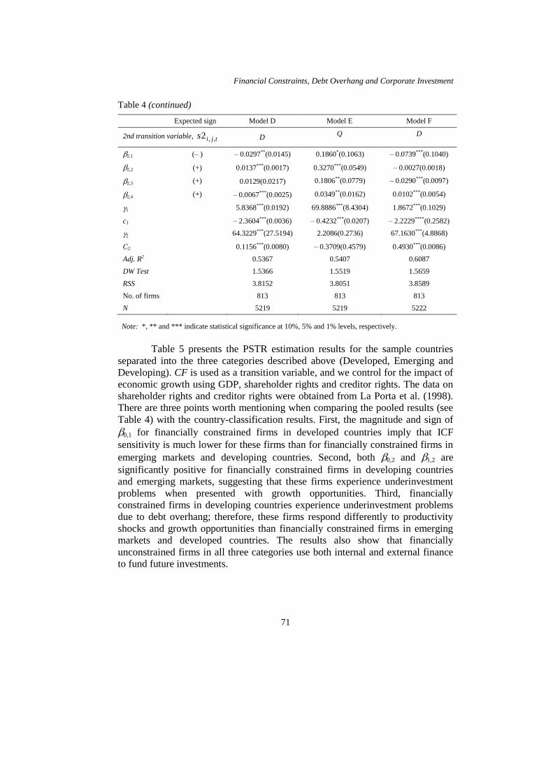
The estimation results for Models D, E and F, which use two transition
functions,13,14
are reported in Table 4. Apparently, there is an increase in the
explanatory power of the models; however, there is also an increase in the value
of the slope parameter 1 . The increase in 1 is higher for Model E than for
Models D and F for the first transition but lower for Model E than for Models D
and F for the second transition. Accordingly, because a higher value of the slope
parameter indicates much faster transitions, the PSTR investment models with
Rashid Ameer
70
two transition functions are not 'optimal' models despite their higher explanatory
powers. Therefore, these results should be interpreted with caution.
Our results show that for Model D, the respective signs of coefficients
CF, Q and D associated with the first transition function (where the transition
variable is CF) are similar to those reported for Model E. However, the respective
signs of coefficients CF, Q and D associated with the second transition function
vary across all models. Our empirical results imply that due to internal cash flow
constraints and debt overhang problems, firms with valuable growth
opportunities face financial constraints; as a result, they decrease their
investments relative to firms without such growth opportunities. This provides
empirical support for the underinvestment problem identified by Islam and
Mozumdar (2007).
Table 4
Panel smooth transition regression estimation – two transition functions
This table reports the estimation results of the PSTR investment model that has two
transition functions (refer to Eq. [5]).
Expected sign Model D Model E Model F
1,0 (– )
– 0.1369***(0.0215) – 0.3215***(0.1030) – 4.7842***(1.7085)
2,0 (+) – 0.0106***(0.0022) – 0.3394***(0.0552) – 7.4835***(1.1662)
3,0 (+) – 0.0194(0.0250) – 0.1575***(0.0781) – 6.6079***(1.6938)
4,0 (+) – 0.0189***(0.0120) – 0.1268***(0.0192) – 0.06523*(0.3365)
1st transition variable, tjis ,,1 CF CF Q
1,1 (– ) 0.1683***(0.0216) 0.1629***(0.0236) 4.8206***(1.7126)
2,1 (+) 0.0143***(0.0026) 0.0125***(0.0026) 7.4828***(1.1660)
3,1 (+) – 0.0485***(0.0132) – 0.0579***(0.0121) 6.6004***(1.6991)
4,1 (+) 0.0887***(0.0126) 0.0959***(0.0128) 0.6546***(0.3383)
(continued on next page)
Financial Constraints, Debt Overhang and Corporate Investment
71
Table 4 (continued)
Expected sign Model D Model E Model F
2nd transition variable, tjis ,,2 D Q D
2,1 (– ) – 0.0297**(0.0145) 0.1860*(0.1063) – 0.0739***(0.1040)
2,2 (+) 0.0137***(0.0017) 0.3270***(0.0549) – 0.0027(0.0018)
2,3 (+) 0.0129(0.0217) 0.1806**(0.0779) – 0.0290***(0.0097)
2,4 (+) – 0.0067***(0.0025) 0.0349**(0.0162) 0.0102***(0.0054)
1 5.8368***(0.0192) 69.8886***(8.4304) 1.8672***(0.1029)
c1 – 2.3604***(0.0036) – 0.4232***(0.0207) – 2.2229****(0.2582)
2 64.3229***(27.5194) 2.2086(0.2736) 67.1630***(4.8868)
C2 0.1156***(0.0080) – 0.3709(0.4579) 0.4930***(0.0086)
Adj. R2 0.5367 0.5407 0.6087
DW Test 1.5366 1.5519 1.5659
RSS 3.8152 3.8051 3.8589
No. of firms 813 813 813
N 5219 5219 5222
Note: *, ** and *** indicate statistical significance at 10%, 5% and 1% levels, respectively.
Table 5 presents the PSTR estimation results for the sample countries
separated into the three categories described above (Developed, Emerging and
Developing). CF is used as a transition variable, and we control for the impact of
economic growth using GDP, shareholder rights and creditor rights. The data on
shareholder rights and creditor rights were obtained from La Porta et al. (1998).
There are three points worth mentioning when comparing the pooled results (see
Table 4) with the country-classification results. First, the magnitude and sign of
0,1 for financially constrained firms in developed countries imply that ICF
sensitivity is much lower for these firms than for financially constrained firms in
emerging markets and developing countries. Second, both 0,2 and 1,2 are
significantly positive for financially constrained firms in developing countries
and emerging markets, suggesting that these firms experience underinvestment
problems when presented with growth opportunities. Third, financially
constrained firms in developing countries experience underinvestment problems
due to debt overhang; therefore, these firms respond differently to productivity
shocks and growth opportunities than financially constrained firms in emerging
markets and developed countries. The results also show that financially
unconstrained firms in all three categories use both internal and external finance
to fund future investments.
Rashid Ameer
72
Table 5
Panel smooth transition regression estimation using alternative sample splits
This table reports the estimation results of the following PSTR investment model (refer to
Eq. [3]).
1 2 3
Coefficients Developed Emerging Developing
1,0 0.0192
(0.0422)
0.0359**
(0.0170)
0.0387*
(0.0235)
2,0 0.0154***
(0.0042)
0.0408***
(0.0105)
0.0501***
(0.0128)
3,0 0.0353***
(0.0149)
– 0.0695*
(0.0377)
– 0.0611
(0.0396)
4,0 – 0.0202***
(0.0109)
0.0314
(0.0321)
0.0317
(0.0318)
1,1 – 0.0732
(0.1060)
– 0.0644***
(0.0272)
– 0.0665***
(0.0313)
2,1 – 0.0139***
(0.1802)
– 0.0497**
(0.0252)
– 0.0571***
(0.0216)
3,1 – 0.0485
(0.0354)
0.0146***
(0.0018)
0.0135*
(0.0786)
4,1 0.0248*
(0.0471)
0.0003
(0.0069)
– 0.0059
(0.0555)
1 10.0319***
(0.9965)
3.347***
(1.5596)
2.2222***
(0.8869)
1c
9.4163***
(0.9530)
0.4298***
(0.0714)
1.0006***
(0.5215)
Control variables
Real_gross domestic product (GDP) 0.0197***
(0.0075)
0.0017*
(0.0009)
0.0009**
(0.0003)
Creditor_rights 0.0003
(0.0001)
– 0.0003
(0.0018)
– 0.0113
(0.0188)
Shareholder_rights 0.0005
(0.0121)
– 0.0001
(0.0001)
– 0.0013
(0.0008)
Adj. R2 0.253 0.069 0.0700
DW test 1.5098 1.8062 1.8022
Firms 412 278 123
N 3221 1628 480
Note: *, ** and *** indicate statistical significance at 10%, 5% and 1% levels, respectively.
Financial Constraints, Debt Overhang and Corporate Investment
73
Heterogeneity and Time Variation of the PSTR Estimated Coefficients
We also examine the heterogeneity and time variation of the estimated
coefficients from a non-linear PSTR model. To this end, we only consider Model
B, i.e., the model that uses the q ratio as a transition variable. We again split the
sample firms into three categories (Developed, Emerging and Developing) to
highlight the economic and financial development that occurred over the period
1991–2010. Figure 2 shows that the q ratio coefficients from the PSTR model are
heterogeneous from one country to another. For instance, when the q ratio is
between 0.5 and 1, the q ratio coefficients are lower for developed countries than
for emerging economies. When the q ratio is between 1.50 and 2, a completely
different trend appears; specifically, the coefficient is higher only for developed
countries. In summary, the heterogeneity of q ratio coefficients proves that the
PSTR model efficiently detects changes in firm-level investment in response to
changes in investment opportunities over the period 1991–2010.
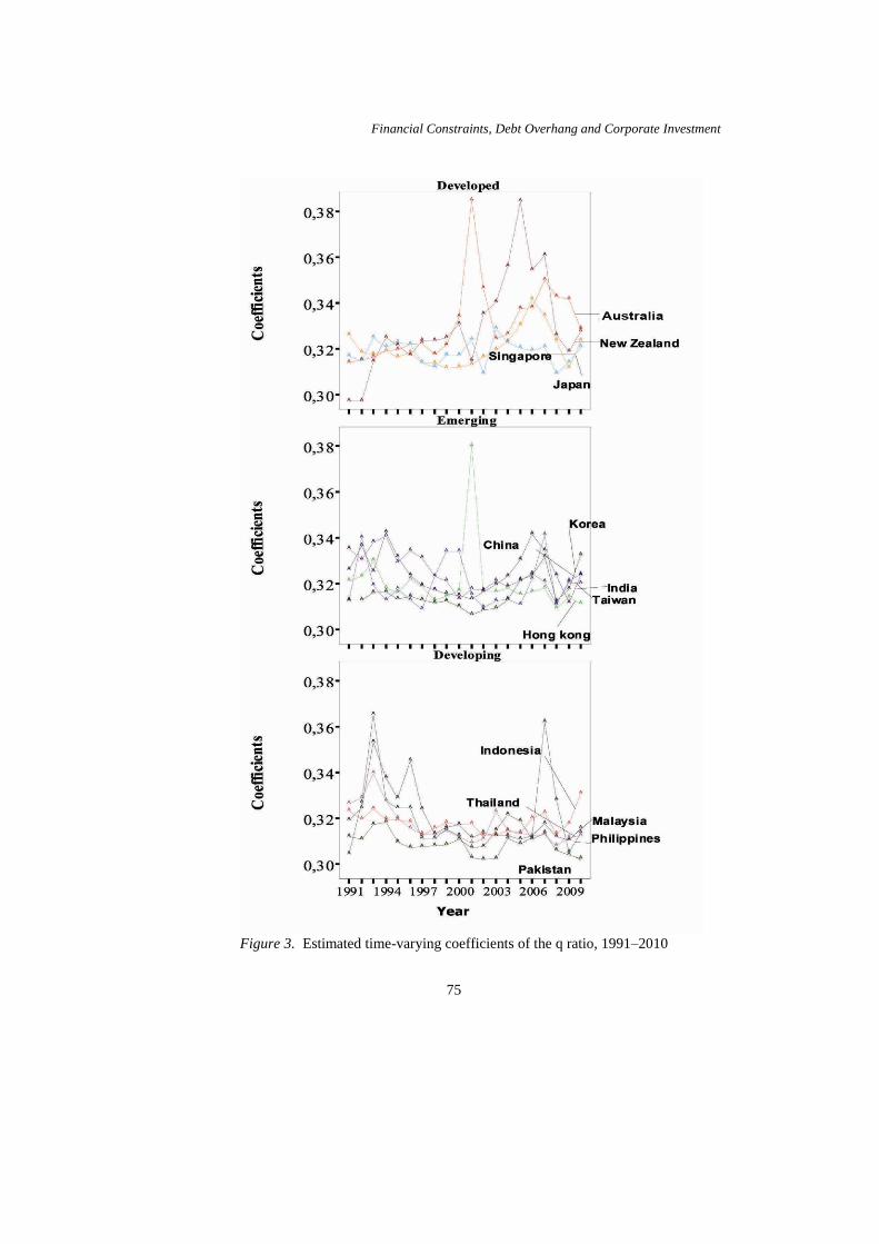
Figure 3 shows the estimated coefficients of the q ratio for each
individual country over the period 1991–2010. These estimates are derived using
the values of the estimated parameters of Model B and the average values of the q
ratio for each country from 1991 to 2010. The estimated coefficients are
remarkably heterogeneous across the three categories of countries. Although the
estimated coefficients for the four developed countries during 1993–1996 are
similar to each other, the curves for Australia and New Zealand take a more
upward direction after 1997 than the curves for Japan and Singapore. For both
emerging markets and developing countries, the estimated coefficient values
were higher during the period of financial reforms (1990–1995) than during other
periods, suggesting that firm-level investments in these economies respond to
new future investment opportunities. This finding is in line with the classical
economics prediction that new investments are valuable only to the extent that
their marginal returns exceed the cost of capital. The results also imply that
higher equity valuations in emerging economies caused a greater increase in firm-
level investment in these areas compared to developing countries. Thus, stock
market liberalisation in emerging economies allows local firms to raise new
capital to invest in new ventures. The more significant decreases in the values of
the estimated coefficients in East Asian countries as a result of the Asian
financial crisis in 1997 shows that the crisis had a greater impact on investment
opportunities in these areas. In addition, the declining values of the coefficients
for developed countries starting in 2007 suggest that the global financial crisis
had a significant effect on firms in these areas; moreover, the recovery in
emerging countries in the Asian region has been faster than the recovery in
developed countries.
Rashid Ameer
74
Figure 2. PSTR coefficients of q ratios
Financial Constraints, Debt Overhang and Corporate Investment
75
Figure 3. Estimated time-varying coefficients of the q ratio, 1991–2010
Rashid Ameer
76
CONCLUSION
This paper investigates the impact of financial constraints on firm-level
investment in 12 Asian countries, Australia and New Zealand. We find evidence
of financial constraints faced by Asian firms and support for the underinvestment
hypothesis reported in previous studies (see, e.g., Aivazian, Ge, & Qiu, 2005).
Our study is the first to use PSTR models to provide strong evidence that firm-
level investment is not sensitive only to cash flow, as advocated by previous
studies. Furthermore, our results suggest that recent studies that use the age or
size of firms as proxies for financial constraints do not properly gauge the levels
of ICF sensitivity in developing countries. Our results show strong heterogeneity
and significant variation in the investment responses to q ratios over time and
across countries. A strong link between investment opportunities and actual
investments in the sample countries suggests that stock market valuations in these
economies are good indicators of future economic growth. We are mindful of the
fact that our results might be sensitive to measurement errors in the q ratio; these
potential measurement errors are not completely eliminated even after controlling
for future profitability and output growth. However, we do not examine the
measurement errors, if there are any, because this issue is beyond the scope of
our paper.
There are certain related empirical questions that are not answered in
this paper that could provide avenues for future research. For example, we do not
segregate firms' fixed-asset investments according to core business operations
and geographical focus. It is probable that export-oriented firms have growth
opportunities that differ from the growth opportunities of import-oriented firms,
and export- and import-oriented firms may have different responses to profit
shortfalls and growth opportunity shocks. In this regard, it would be useful to
examine the influence of foreign trade exposure at the firm-level. In addition, the
monopoly power of firms in some Asian countries allows them to secure
favourable access to external finance. It would be useful to identify the link
between market power and firm-level investment. Furthermore, it has been
shown in the asset pricing literature that financial constraints affect risk and
expected returns (Livdan, Sapriza, & Zhang, 2009). A follow-up study using an
Asian sample could have implications for foreign fund managers.
NOTES
1. In some cross-country regressions, indicators of financial development at the
macro level have been used to divide samples of firms into developed and less
developed markets to test ICF sensitivities across countries (see Islam &
Mozumdar, 2007; Love, 2003; Wurgler, 2000).
Financial Constraints, Debt Overhang and Corporate Investment
77
2. Variables that have been used to separate firms into groups of constrained and
unconstrained firms include gross cash flow (Brown & Petersen, 2009;
Almeida & Campello, 2007) and net sales (Laeven, 2003). Schiantarelli
(1996) provides a useful review of the methodological issues associated with
time-invariant classifications and the use of proxy variables.
3. Several studies that have included Asian countries are Islam and Mozumdar
(2007, Love (2003) and Laeven (2003).
4. Minton and Schrand (1999) argue that higher cash flow volatility implies that
a firm is more likely to have periods of cash flow shortages, and a firm may
forgo investment if additional finance is only available at a higher cost.
Consequently, firms that rely more on external capital than on internal capital
will decrease future investment.
5. Using a sample of Compustat firms and measuring growth with several proxy
variables (e.g., increase in capital expenditure), Lang et al. (1996) find that
leverage reduces US firms' growth only for firms with low q ratios. Likewise,
Hu and Schiantarelli (1998) report that U.S. firms with high debt ratios are
more sensitive to the availability of internal funds. Cai and Zhang (2011,
p. 392) report that an increase in the leverage ratio is associated with lower
real investment in the future. Specifically, they find that a 10% increase in the
leverage ratio in the current quarter on average is associated with a 6.23%
reduction in the investment rate in the next four quarters.
6. The first variable (Structure-Activity) equals the log of the ratio of Value
Traded to Bank Credit. Value Traded equals the value of stock transactions as
a share of national output. Bank Credit equals the claims of the banking sector
on the private sector as a share of GDP. The second variable (Structure-Size)
equals the log of the ratio of Market Capitalization to Bank Credit. Market
Capitalization is defined as the value of listed shares divided by GDP (Beck &
Levine, 2002, p. 147).
7. The logistic smooth transition autoregressive model (LSTAR) has been used
by Terasvirta and Anderson (1992) to characterise the dynamics of industrial
production indexes in a number of OECD countries during expansions and
recessions.
8. According to Gonzalez et al. (2005), a variable that strongly rejects the
linearity test (as determined using the p-value of the linearity test statistic,
LMF) is an ideal transition variable.
9. See the technical appendix in Gonzalez et al. (2005) for this procedure.
10. The PSTR investment model is a non-linear model because the transition
function is multiplied by right-hand side variables.
Rashid Ameer
78
11. The q ratio and the debt ratio are used in transition functions by Gonzalez
et al. (2005) and Hu and Schiantarelli (1998).
12. In other models, such as Models A and C, the values of the slope parameter
are higher, which implies that the transition function is sharp and might
correspond to an indicator function, as suggested by Fouquau et al. (2008).
13. Transition function estimated from the Model A corresponds to an indicator
function.
14. Although Model D explains more than 50% of the variation in firms'
investments, it has higher values for the slope parameters 1 and 2; thus, the
results of Model D are weaker than the results of Model B.
REFERENCES
Abel, A. B., & Eberly, J. C. (1994). A unified model of investment under uncertainty.
American Economic Review, 84(5), 1369–1384.
Agca, S., & Mozumdar, A. (2008). The impact of capital market imperfection on
investment-cash flow sensitivity. Journal of Banking and Finance, 32(2), 207–216.
Agung, J. (2000). Financial constraint, firm's investment and the channels
of monetary policy in Indonesia. Applied Economics 32(13), 1637–1646.
Aivazian, V. A., Ge, R., & Qiu, J. (2005). The impact of leverage on firm investment:
Canadian evidence. Journal of Corporate Finance, 11(1–2), 277–291.
Almeida, H., & Campello, M. (2007). Finanical constraints, asset tangibility, and corporate
investment. The Review of Financial Studies, 20(5), 1429–1460.
Barnett, S., & Sakellaris, P. (1998). Nonlinear response of firm investment to Q. Testing
a model of convex and non-convex adjustment costs. Journal of Monetary
Economics, 32(2), 261–288.
Beck, T., & Levine, R. (2002). Industry growth and capital allocation: Does having a
market- or bank-based system matter? Journal of Financial Economics, 64(2),
147–180.
Bekaert G., & Harvey, C. (2000). Foreign speculators and emerging equity markets. The
Journal of Finance, 55(2), 565–613.
Bekaert, G., Harvey, C., & Lundblad, C. (2005). Does financial liberalization spur
growth? Journal of Financial Economics, 77(1), 3–55.
Bond, S., Klemm, A., Newton-Smith, R., Syed, M., & Vlieghe, G. (2004). The roles of
expected profitability, Tobin's Q and cash flow in econometric models of company
investment (Working Paper). Washington, DC: The Institute for Fiscal Studies,
Brookings Institution.
Bond, S., & Meghir, C. (1994). Dynamic investment models and the firm's financial
policy. The Review of Economic Studies, 61(2), 197–222.
Brown, J., & Petersen, B. (2009). Why has the investment-cash flow sensitivity declined
so sharply? Rising R&D and equity market developments. Journal of Banking and
Finance, 33(5), 971–984.
Financial Constraints, Debt Overhang and Corporate Investment
79
Campello, M., Graham, J., & Harvey, C. R. (2009). The real effect of financial
constraints: Evidence from a financial crisis (NBER Working Paper 1552).
Washington, DC: Brookings Institution.
Cleary, S. (2006). International corporate investment and the relationships between
financial constraint measures. The Journal of Banking and Finance, 30(5), 1559–
1580.
Erickson, T., & Whited, T. (2000). Measurement error and the relationship between
investment and Q. Journal of Monetary Economics, 108(51), 1027–1057.
Fazzari, S. R., Hubbard, G., & Petersen, B. (1988). Finance constraints and corporate
investment. Brookings Paper on Economic Activity, 1(1), 141–195.
Fouquau, J. Hurlin, C., & Rabaud, I. (2008). The Feldstein-Horioka puzzle: A panel
smooth transition regression approach. Economic Modelling, 25(2), 284–299.
Galindo, A., Schiantarelli, F., & Weiss, A., (2005). Does financial liberalization improve
the allocation of investment? Micro evidence from developing countries. Journal
of Development Economics, 83(2), 562–587.
González, A., Teräsvirta, T., & Dijk, D. (2005). Panel smooth transition regression
model, SSE/EFI Working Paper Series in Economics and Finance 604, Stockholm
School of Economics. Retrieved 2 December 2005 from http://swopec.hhs.se/
hastef/ papers/hastef0604.pdf
Hansen, B. E. (2000). Sample splitting and threshold estimation. Econometrica, 68(3),
575–603.
Harris, J. Schiantarelli, F., & Siregar, M. G. (1994). The effect of financial liberalization
on capital structure and investment decisions of Indonesian manufacturing
establishments. The World Bank Economic Review, 8(1), 17–47.
Hennessy, C A. (2004). Tobin's Q, debt overhang, and investment, The Journal of
Finance 59(4), 1717–1742.
Hoshi, T., Kashyap, A., & Scharfstein, D. (1991). Corporate structure, liquidity, and
investment: Evidence from Japanese industrial groups. The Quarterly Journal of
Economics, 106(1), 33–60.
Hu, X., & Schiantarelli, F. (1998). Investment and capital market imperfections: A
Switching regression approach using U.S. firm panel data. The Review of
Economics and Statistics, 80(3), 466–479.
Hubbard, G. (1998). Capital market imperfections and investment. Journal of Economic
Literature, 36(1), 198–225.
Islam, S. S., & Mozumdar, A. (2007). Financial development and the importance of
internal cash: Evidence from international data. Journal of Banking and Finance,
31(3), 641–658.
Jaramillo, F., Schiantarelli, F., & Weiss, A. (1996). Capital market imperfections before
and after liberalization: An Euler equation approach to panel data for Ecuadorian
firms. Journal of Development Economics, 51(2), 367–386.
Kaplan, S. N., & Zingales, L. (1997). Do financing constraint explain why investment is
correlated with cash flow? Quarterly Journal of Economics, 112(1), 169–215.
Laeven, L. (2003). Does financial liberalization reduce financing constraints? Financial
Management, 32(1), 5–34.
Livdan, D., Sapriza, H., & Zhang, L. (2009). Financially constrained stock return. The
Journal of Finance, 64(4), 1827–1862.
Rashid Ameer
80
Love, I. (2003). Financial development and financing constraints: International evidence
from the structural investment model. The Review of Financial Studies, 16(3),
765–791.
Minton, B.A., & Schrand, C. (1999). The impact of cash flow volatility on discretionary
investment and the costs of debt and equity financing. Journal of Financial
Economics, 54(3), 423–460.
Morgado, A., & Pindado, J. (2003) The under and over-investment hypothesis: An
analysis using panel data. European Financial Management, 9(2), 163–177.
Myers, S. C. (1977). Determinants of corporate borrowing. Journal of Financial
Economics, 5(2), 147–175.
Schmukler, L., & Vesperoni, S. (2002). Short-run pain, long-run gain: The effects of
liberalization, Policy Research Paper, International Monetary Finance Working
Paper 03/34. Washington DC: International Monetary Fund.
Whited, T. M. (1992). Debt, liquidity constraints, and corporate investment: Evidence
from panel data. The Journal of Finance, 47(4), 1425–1460.
Wurgler, J. (2000). Financial markets and allocation of capital. Journal of Financial
Economics, 58(1–2), 187–214.