This article was downloaded by: [University of Saskatchewan Library] On: 24 September 2012, At: 00:30 Publisher: Routledge Informa Ltd Registered in England and Wales Registered Number: 1072954 Registered office: Mortimer House, 37-41 Mortimer Street, London W1T 3JH, UK Quantitative Finance Publication details, including instructions for authors and subscription information: http://www.tandfonline.com/loi/rquf20 Financial crisis dynamics: attempt to define a market instability indicator Youngna Choi a & Raphael Douady b a Department of Mathematical Sciences, Montclair State University, Montclair, NJ 07043, USA b CNRS, Centre d'Economie de la Sorbonne, Univ. Paris I, Riskdata, 6 Rue de l'Amiral de Coligny, 75001 Paris, France Version of record first published: 06 Feb 2012. To cite this article: Youngna Choi & Raphael Douady (2012): Financial crisis dynamics: attempt to define a market instability indicator, Quantitative Finance, 12:9, 1351-1365 To link to this article: http://dx.doi.org/10.1080/14697688.2011.627880 PLEASE SCROLL DOWN FOR ARTICLE Full terms and conditions of use: http://www.tandfonline.com/page/terms-and-conditions This article may be used for research, teaching, and private study purposes. Any substantial or systematic reproduction, redistribution, reselling, loan, sub-licensing, systematic supply, or distribution in any form to anyone is expressly forbidden. The publisher does not give any warranty express or implied or make any representation that the contents will be complete or accurate or up to date. The accuracy of any instructions, formulae, and drug doses should be independently verified with primary sources. The publisher shall not be liable for any loss, actions, claims, proceedings, demand, or costs or damages whatsoever or howsoever caused arising directly or indirectly in connection with or arising out of the use of this material.
Transcript
This article was downloaded by: [University of Saskatchewan Library]On: 24 September 2012, At: 00:30Publisher: RoutledgeInforma Ltd Registered in England and Wales Registered Number: 1072954 Registered office: MortimerHouse, 37-41 Mortimer Street, London W1T 3JH, UK
Quantitative FinancePublication details, including instructions for authors and subscription information:http://www.tandfonline.com/loi/rquf20
Financial crisis dynamics: attempt to define a marketinstability indicatorYoungna Choi a & Raphael Douady ba Department of Mathematical Sciences, Montclair State University, Montclair, NJ 07043,USAb CNRS, Centre d'Economie de la Sorbonne, Univ. Paris I, Riskdata, 6 Rue de l'Amiral deColigny, 75001 Paris, France
Version of record first published: 06 Feb 2012.
To cite this article: Youngna Choi & Raphael Douady (2012): Financial crisis dynamics: attempt to define a marketinstability indicator, Quantitative Finance, 12:9, 1351-1365
To link to this article: http://dx.doi.org/10.1080/14697688.2011.627880
PLEASE SCROLL DOWN FOR ARTICLE
Full terms and conditions of use: http://www.tandfonline.com/page/terms-and-conditions
This article may be used for research, teaching, and private study purposes. Any substantial or systematicreproduction, redistribution, reselling, loan, sub-licensing, systematic supply, or distribution in any form toanyone is expressly forbidden.
The publisher does not give any warranty express or implied or make any representation that the contentswill be complete or accurate or up to date. The accuracy of any instructions, formulae, and drug dosesshould be independently verified with primary sources. The publisher shall not be liable for any loss, actions,claims, proceedings, demand, or costs or damages whatsoever or howsoever caused arising directly orindirectly in connection with or arising out of the use of this material.
Quantitative Finance, Vol. 12, No. 9, September 2012, 1351–1365
Financial crisis dynamics: attempt to define a market
instability indicator
YOUNGNA CHOIy and RAPHAEL DOUADY*z
yDepartment of Mathematical Sciences, Montclair State University, Montclair, NJ 07043, USAzCNRS, Centre d’Economie de la Sorbonne, Univ. Paris I, Riskdata, 6 Rue de l’Amiral de Coligny,
75001 Paris, France
(Received 12 December 2009; revised 7 February 2011; in final form 22 August 2011)
The impact of increasing leverage in the economy produces hyperreaction of marketparticipants to variations of their revenues. If the income of banks decreases, they mass-reducetheir lendings; if corporations sales drop, and they cannot adjust their liquidities by furtherborrowing due to existing debt, then they must immediately reduce their expenses, lay off staff,and cancel investments. This hyperreaction produces a bifurcation mechanism, and eventuallya strong dynamical instability in capital markets that is commonly called systemic risk. In thisarticle, we show that this instability can be monitored by measuring the highest eigenvalue of amatrix of elasticities. These elasticities measure the reaction of each sector of the economy to adrop in its revenues from another sector. This highest eigenvalue—the spectral radius—of theelasticity matrix can be used as an early indicator of market instability and potential crisis.Grandmont and subsequent research showed the possibility that the ‘invisible hand’ ofmarkets becomes chaotic, opening the door to uncontrolled swings. Our contribution is toprovide an actual way of measuring how close to chaos the market is. Estimating elasticitiesand actually generating the indicators of instability will be the topic of forthcoming research.
Keywords: Systemic risk; Econophysics; Macroeconomics; Bifurcation; Contagion; Dynamicalsystems; Chaos theory
The global aspect of the subprime-originated financialcrisis in 2007–09þ is the contagion of risks, which is betterdescribed by the butterfly effect, which started regularlybeing mentioned after the series of financial ‘unthink-ables’ that took place in September 2008, starting with thenationalization of government-sponsored enterprisesFreddie Mac and Fannie Mae, the demise of theinvestment bank Lehman Brothers a week later, the fire-sale of another one, Merrill Lynch, to Bank of Americaon the same day, and the government bailout of theinsurance giant AIG just two days later.
The ‘butterfly effect’ is a term used to describe aphenomenon such that small changes at the initial stageresult in a huge difference in long-term behavior.The 2007–09þ financial crisis started in the U.S.real estate market and spread all over the world.
Such a phenomenon is formally defined in dynamical
systems as a sensitive dependence on initial conditions.
When a dynamical system possesses a sensitive depen-
dence on initial conditions together with cyclical behav-
ior, the system often exhibits chaos (Palis and de
Melo 1982).In dynamical systems theory, a bifurcation refers to a
structural modification of the system behavior upon a
continuous change in the parameters of its equations. A
catastrophe occurs when, following a bifurcation, a small
change in the parameters discontinuously alters the
equilibrium state of the economy. During the 2007–09þ
subprime crisis we did observe such a catastrophic event,
where a mild evolution of economic parameters ended in a
drastic shift in financial interactions. On the brink of the
crisis, the economy was in what physicists call a ‘meta-
stable equilibrium’, i.e. an equilibrium state that is
destroyed by a very small perturbation—like a dry
forest totally burning upon the scratch of a match—
leading to a series of catastrophic events, until another*Corresponding author. Email: [email protected]
Quantitative FinanceISSN 1469–7688 print/ISSN 1469–7696 online � 2012 Taylor & Francis
basin of attractiony is reached, i.e. another stationaryevolution mode, another cycle, or even a strange attractoras chaos theory may predict.
Although the economy as a whole is a very complexbody (system) that is hard to describe as a finite-dimensional dynamical system, its behavior during thecrisis leads us to state the hypothesis that its major driverscan be described by such a system.
In this paper we suggest that the 2007–09þ financialcrisis was mainly caused by a breakdown of the dynamicstability of the financial system, according to somecatastrophic mechanism. More precisely, we start froma mathematical model of the flows of funds in thefinancial system that exhibits a stationary state equilib-rium. The dimension n of the model is the number ofaggregate agents, specified in the next section. Thefinancial activities are considered as continuous pertur-bations of this equilibrium: when the perturbation is smallenough and the equilibrium is stable, the equilibriumpersists and the economy remains stable. When theperturbation is too big or if the equilibrium becomesunstable, it collapses and a financial crisis occurs.Furthermore, we show that the critical size of perturba-tions that destroy the equilibrium shrinks when financialactors react more rapidly and intensely to other actorswith whom they have business relations, leading to ameta-stable equilibrium and a catastrophe. We call thesespeeds of reaction elasticities. The critical perturbationsize is directly related to the debt and borrowing capacity,the leverage, and the market liquidity. In other words, ourmathematical model shows a relation between leverageand market instability.
Based on these observations, we propose the principlesof a methodology to build an early indicator of the globalsystem instability. The details of such an indicator stillneed to be worked out and tested, using readily availablemacroeconomic data such as those of Federal Reserve(2011a). In particular, the definition of aggregate agentsmay differ depending on the geographic and economiccontext. Estimating elasticities and actually generating theindicators of instability will be the topic of forthcomingresearch.
Since the liquidity freeze following Lehman Brothers’collapse, many research articles on financial crises andsystemic risk, both theoretical and empirical, have beenwritten. However, there are earlier papers that share ourperspective. Minsky’s classic The Financial InstabilityHypothesis (FIH) (Minsky 1992) is about the impact ofdebt on system behavior. According to FIH, there are tworegimes of financing, stable and unstable, and after aperiod of prolonged prosperity, the economy switchesfrom the former to the latter by shifting the weights offinancing schemes labeled as hedge finance, speculativefinance, and Ponzi finance. This framework, albeit writtenalmost 20 years ago, explains amazingly well the formingof the 2007–09þ financial crisis. Benhabib et al. (2006)
studied multisector real business cycle models and foundthat the three-sector model has a strong propagation—aprelude to contagion—mechanism. Several recent papershave an interpretation of financial crises similar to that ofthe authors: the uncontrolled proliferation of financialinstruments erodes systemic stability and leads the marketto a susceptible critical condition with enhanced correla-tions (Caccioli et al. 2009); the loss of confidence spreadsthroughout the interbank network structure, and this anddebt maturity mismatches contribute to systemic financialcrises (Anand et al. 2011); the 2007–09þ global financialcrisis is modeled as an optimization by the financial agentswith a combination of shocks—burst of the housingbubble, the increased cost of borrowing, decreased con-sumption, and government policy (McKibbin and Stoeckel2009); and a heavily leveraged investment demonstratesheavy-tailed price fluctuations, and margin calls force thesale of funds in a falling market whose consequentnonlinear feedback amplifies price decreases (Thurner etal. 2010). One can find a general overview of agent-basedmodels in Hommes (2008). Helbing (2010) gives a sum-mary of how complexity contributes to the emergence ofsystemic risks in socio-economic systems, and large-scaledisasters are mostly based on cascading effects due tononlinear and/or network interactions.
The rest of the paper is organized as follows. In section2 we provide an intuitive view of the chaos in the 2007–09þ financial crisis and the relevant mathematics back-ground. Section 3 is fully devoted to the structuralstability and perturbation analysis of the financial system.Section 4 introduces the market instability indicator.Section 5 is devoted to the bifurcation that causes afinancial crisis, its aftermath, and the chaotic behavior inthe default mechanism. More complicated mathematicsare explained in detail in the appendices.
2. Glimpse of chaos
Avoiding the question of pricing model validity,which appears to us as a side question, we try tounderstand the financial, then economic crisis in itsdynamical aspects.
2.1. Brief recollection of the 2007–2009þ crisis
A financial crisis is generally defined as a situation inwhich some financial institutions or assets suddenly lose alarge part of their value. The 2007–2009þ crisis started ina small sector of the global economy called ‘the U.S. realestate market’. In the United States the housing bubblestarted to form in 2000–01, following the burst ofthe tech bubble in spring 2000 and the September 11events. After the Federal Reserve’s rate cut and thedevelopment of securitization (CDO, MBS) and creditderivatives (CDS),z a lot of money was made
yThe basin of attraction of an equilibrium of a dynamical system f is the open set of points whose trajectory converges to theequilibrium under the iteration of f.zCollateralized debt obligation, mortgage-backed security, and credit default swap.
1352 Y. Choi and R. Douady
Dow
nloa
ded
by [
Uni
vers
ity o
f Sa
skat
chew
an L
ibra
ry]
at 0
0:30
24
Sept
embe
r 20
12
available for lending (housing, consumers, corporations,etc.). These drove interest rates down, both T-bondsand corporate spreads, which resulted in a bond rally.That induced capital inflow into securitized products thatappeared to investors as risk-free assets with excessreturn with respect to the money market. Therefore,even more money was made available, and this feedbackloop created the credit bubbles. In parallel, privateequity investors and venture capitalists who lost a lot inthe crash of the NASDAQ in 2000 had to deliver returnsto their investors and started becoming short-termists.A large portion of the investment in small andmedium companies was done through LBO.yThe increasing debt of companies in general made theirbalance sheets more and more sensitive to the level ofcredit spreads. As long as credit spreads were going down,corporations could refinance themselves, but the smallestloss of confidence from lenders would (and did) put themin a financial squeeze. In the real sector, many peoplestarted investing in real estate. The Case–Shiller HomePrice Index had its peak in the second quarter of 2006(S&P/Case-Shiller 2011), and U.S. house prices havedrastically decreased since. Many banks and financialentities, both regional and global, went bankrupt (BBCNews 2008; Federal Deposit Insurance Corporation2011). Companies, both small and large, went under aswell (Altman and Karlin 2010). In both cases the maincause was the lack of solvency and liquidity. During thedevelopment of the crisis, the damage seemed to bebecoming more severe, massive, and unpredictable, withquestions about a ‘double dip’. Three years after the peakof the crisis—the bankrupcy of Lehman Brothers—thecurrent situation seems to be stabilizing, but the futurestill looks unpredictable, due to the increasing sovereigndebt of major countries.
Here we get a glimpse of chaos: what started locallyhas spread globally with unpredictable severity. Thisdemonstrates a sensitive dependence on initial conditions.The mathematical models that used to work well in thepast, all of a sudden do not work any longer, and thishappens when a dynamical system experiences abifurcation.
Typically, chaos is found in dynamical systems thatpossess non-trivial recurrence (i.e. which cannot beisolated), and indeed there is a ‘recurrence of risks’behind the 2007–09þ financial crisis. In dynamicalsystems theory, recurrence appears when forces keep thesystem within a confined area of the ‘phase space’. Thetypical road to chaos is as follows.
. A bifurcation breaks the stability of someequilibrium.
. Through a catastrophe the asymptotic behaviorsuddenly shifts from the formal equilibrium tocompletely different behavior.
. When recurrence occurs, symbolic dynamicstakes place and the asymptotic behavior ischaotic.
For instance, securitization was one of the causes thatcreated a bifurcation and eventually chaos. Although theoriginal purpose of the securitization was to diversifydefault risk, this ‘originate to distribute’ practice spawnedtoo many risky loans that were destined to default. As aresult the risk was disseminated globally as opposed todiversified, then boomeranged back to the issuer of theloans as well as to the borrowers. This is because allthe financial transactions were made in a closed system. Ifthe Masters of the Universe on our planet had managedto pass all those risks to other denizens of the universe, wewould not be having any of the problems we are havingnow, for the Earth would aggregately act as a source ofrisks. For instance, the case of local systemic crises, suchas the Asian–Russian one in 1997–98, was very differentfrom that of 2007–09þ and eventually was rapidlyabsorbed.
2.2. Introduction of the agent
We consider an economy divided into n large aggregates,which we assume to act as economic agents, possiblyheterogeneous. At each time t, we observe the wealthvector w(t)¼ (w1(t), . . . ,wn(t))2R
n representing then-tuple of agents’ wealth. The number n of agents maydiffer, depending on which economy is being studied.
We make two assumptions on the system.
. Minimality: Any removal of an agent wouldmake the system collapse, as other agents wouldnot be able to function without it. Thesame would occur if the wealth of one of theagents vanishes: in this case, other agents wouldnot be able to interact and their wealth woulddecrease to zero as well. As a consequence,we can assume that economic agents actingoptimally will take steps so as to prevent suchan event.
. Boundedness: The economy is based on limitedmaterial resources and market participants,therefore production and consumptionare bounded from above. We express thisassumption mathematically by saying that thewealth of a given agent cannot exceed alimited number of times the sum of the wealthof other agents. Equivalently, we say that thereis a time adjustment factor �(t) such thatthe wealth of any agent, divided by this adjust-ment factor, remains bounded from above,while the adjusted total wealth of the economy(sum of agents’ wealth divided by the adjust-ment factor) remains bounded from below. Thetime adjustment may differ from inflation andis intuitively related to the growth of theeconomy.
These two assumptions together are equivalent tosaying that the ratio of wealth between any two agents
yLeveraged buyout.
Financial crisis dynamics 1353
Dow
nloa
ded
by [
Uni
vers
ity o
f Sa
skat
chew
an L
ibra
ry]
at 0
0:30
24
Sept
embe
r 20
12
remains bounded. As a result, the evolution of wealth inconstant dollars, i.e. normalized by �(t), is confined in acompact set M�R
n.To model the 2007–2009þ financial crisis that started in
the U.S. real estate market, let us now broadly divide theeconomy into several segments in the spirit of Benhabibet al. (2006). Typically, home buyers (HB), who we do notdistinguish from general consumers, obtain financingfrom local mortgage lenders (ML), which includes themortgage divisions of large banks. To facilitate financingwith limited funds, these mortgages are sold to largebanks (LB; not only banks, but other financial institu-tions that function like banks, for example brokers andinsurance companies) and government-sponsored enter-prises (GSE; Fannie Mae and Freddie Mac) for securi-tization—they are sliced, diced, and repackaged asmortgage-backed securities (MBS), which are a specialkind of asset-backed securities (ABS) or collateralizeddebt obligations (CDO). Part of these MBSs are keptwithin the banks (super-senior tranches) or are securitizedagain (ABS-squared) and sold in the secondary mortgagemarket. They are also sold to investors. The investors (I)consist of many funds from all over the world, such aspension funds, mutual funds, academic endowments, stateemployees’ retirement funds, sovereign funds, etc. Thewealth of many people, directly and indirectly, dependson such funds, so the impact of these funds on the realsector of the economy is immense.
As for speculative hedge funds, they are indeed animportant segment of the financial system to understandits short-term reactions. They act as liquidity providersand sometimes destabilize the whole system. However,they are rarely solely responsible for financial bubbles. Inour framework, due to lack of data for this segment, wedecided to merge them with the general investors’ class ‘I’,as this does not significantly affect the overall behavior ofthe model.
Another key player in the real sector is corporations (C).Home buyers pay their loan installments to mort-gage lenders and large banks, and they do so largelythanks to the wages paid mostly by corporations, which, inreturn, are financed mostly by large banks and investors.
We have also separated the government from otherfinancial actors, as we wish to understand the dynamics of
the free market. Government actions, when they occur,are directed mainly at banks and government-sponsored
enterprises, and indirectly at corporations and consumersby the fiscal policy or industrial programs. The frame-
work we describe here provides a clear basis to under-
stand the potential impact of such government actions.
2.3. At-will and scheduled cash flows
The cash flows among these six segments, HB, ML, LB,
GSE, C, and I, can be further classified into two groups,‘variable’ cash flows and ‘fixed’ cash flows. ‘Variable’
cash flows include equity investments, debt investments(commonly called loans), and dividends, which include
payments that act like dividends. Generally speaking, all
cash flows are at will (figure 1).
(1) Equity investments:
(a) HB to HB: home buyers invest in houses, and
sell them to one another.(b) C to C: companies invest in each other.(c) I to LB, GSE, and C: investors buy stocks of
LB, GSE, and C.
(2) Loans (debt investments):
(a) ML to HB: mortgage loans.(b) LB to HB: credit cards and other financing,
LB to ML: purchasing mortgages for securiti-
zation,LB to LB and GSE: secondary MBS market,
LB to C: bank loans to companies.(c) GSE to ML and LB: guarantees mortgages by
purchasing them and creating MBS.(d) I to LB, GSE, and C: investors buy bonds
issued by LB, GSE, and C.
(1) Dividends:
(a) LB, GSE, and C to I: investors earn dividends
from LB, GSE, and C stocks they invested in.
GSE
3(a)
2(b)
LB
C1(b)
I1(c), 2(d)1(a) 2(a) 2(b)
2(c) 2(c) 2(b)
2(b)
3(b)
3(a)
1(c), 2(d)
HB ML
3(a)
2(b)
41(c), 2(d)
Figure 1. Variable cash flows among six agents.
1354 Y. Choi and R. Douady
Dow
nloa
ded
by [
Uni
vers
ity o
f Sa
skat
chew
an L
ibra
ry]
at 0
0:30
24
Sept
embe
r 20
12
(b) I to HB: investors pay pensions to their clients,which work like dividends.
(4) Consumption: HB to C.
‘Fixed’ cash flows are ‘coupons’, which include not onlybond coupons, but payments from fixed-rate mortgagesand other conventional loans, minimum payments foradjustable-rate mortgages and credit card loans, salaries,and contributions to retirement funds and other moneymarket funds. Also included are premiums for creditdefault swaps (CDS) to issuing financial institutions fromcounterparties. Generally speaking, these are all scheduledcash flows (figure 2).
(5) Coupons:
(a) HB to ML and LB: mortgage and otherfinancing payments, credit card debtpayments.
(b) ML to LB and GSE: although LB and GSEpurchase mortgages from ML for securitiza-tion and guarantee them by holding theresulting MBS, the payments from HB arestill directly made to the original lender ML.So we interpret a cash flow from ML to GSEand LB.
(c) LB to LB, GSE, and I: coupons for MBS andABS of MBS markets. Also included are CDSpremiums.
(d) GSE to LB and I: GSE pays coupons to MBSinvestors. When GSE started buying andguaranteeing more MBSs the financial crisishad already developed (Chung et al. 2008). Weconsider cash flows during the normal econ-omy, so do not include this special case whichwill create a loop from GSE to itself.
(e) C to LB and I: companies pay coupons to thebond holders.
(6) Salary: C to HB.(7) Contributions (e.g. pension funds): HB to I.
In fact, both types of cash flows are impacted byeconomic conditions, the less variable ones not necessarilybeing those called ‘fixed’. For example, the cash flow from
households to industry in exchange for basic goods andservices remains almost constant regardless of the eco-nomic conditions. Non-interest income for banks such asATM fees and credit card fees are not affected byeconomic deterioration, since banks can always raisethem. Such cash flows are rather steady, while paymentsfrom subprime loans, which are subject to default, are inpractice more variable cash flows.
At a macroeconomic level, variations of aggregate cashflows can be explained by shifts in the classical Hick’s IS-LM curves. However, in order to assess the actual marketstability, we do not deduce variations of cash flows from amodel, but from empirical observations. Market instabil-ity, which is the core target of our study, may possiblyresult from behavior that is predicted by a model (e.g.,Grandmont (1985)), but it may also well be the conse-quence of the economy departing from classical models.
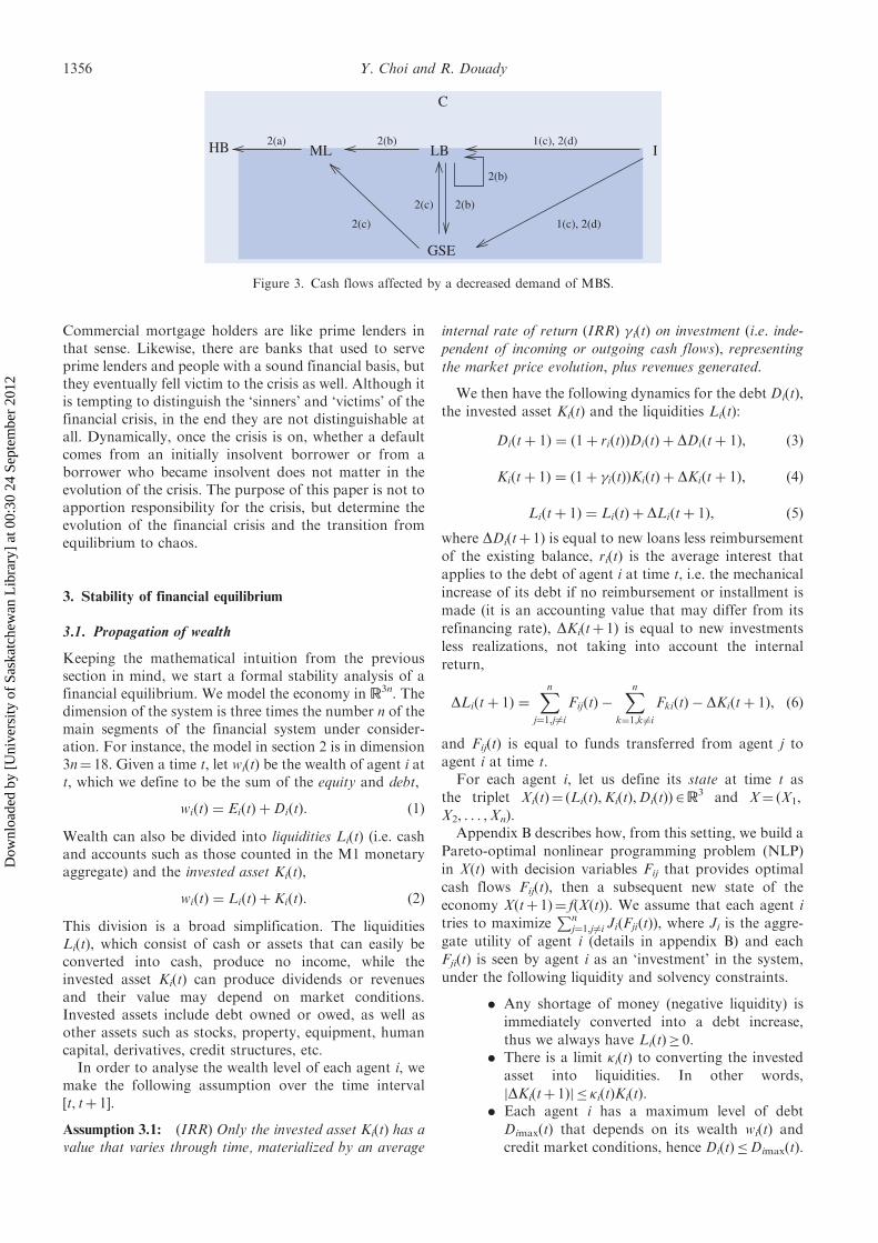
When the real estate bubble burst in 2007, home buyersstarted getting behind with their payments. So thefinancial segments at the receiving end of cash flowsinvolving MBS experienced significant default and writedowns (figure 3), which lead to the bailout of Fannie Maeand Freddie Mac in September 2008. The blow was moresevere for large banks, since they not only invested inthose CDOs, but also insured against them by sellingCDSs. Just a week later, Lehman Brothers declaredbankruptcy and Merrill Lynch was sold to Bank ofAmerica on the same day. Several days later, theinsurance giant AIG was bailed out.
The September 2008 saga froze market liquidity andcorporations started having trouble obtaining credit. Thisresulted in the mass bankruptcy of companies of all sizes,and consequently massive unemployment. The marketvalues of companies and banks plunged, and so did thereturns to the investors and the home buyers whocontributed to them. This resulted in ‘victims’ of thefinancial crisis. In the U.S. real estate market, not allhome buyers contributed to the crisis. There are peoplewho used to be prime borrowers and never previouslydelinquent with their payments, but ended up fallingbehind due to the side-effects of the financial crisis, suchas plunging house prices, soaring interest rates on loans,and job loss (Bullock and Scholtes 2009, Singh 2009).
GSE
5(d)
5(c)
LB
C
I5(a) 5(b)
5(b) 5(d) 5(c)
5(e)
7
5(c)HB ML
5(e)
5(a)
6
Figure 2. Fixed cash flows among six agents.
Financial crisis dynamics 1355
Dow
nloa
ded
by [
Uni
vers
ity o
f Sa
skat
chew
an L
ibra
ry]
at 0
0:30
24
Sept
embe
r 20
12
Commercial mortgage holders are like prime lenders inthat sense. Likewise, there are banks that used to serveprime lenders and people with a sound financial basis, butthey eventually fell victim to the crisis as well. Although itis tempting to distinguish the ‘sinners’ and ‘victims’ of thefinancial crisis, in the end they are not distinguishable atall. Dynamically, once the crisis is on, whether a defaultcomes from an initially insolvent borrower or from aborrower who became insolvent does not matter in theevolution of the crisis. The purpose of this paper is not toapportion responsibility for the crisis, but determine theevolution of the financial crisis and the transition fromequilibrium to chaos.
3. Stability of financial equilibrium
3.1. Propagation of wealth
Keeping the mathematical intuition from the previoussection in mind, we start a formal stability analysis of afinancial equilibrium. We model the economy in R
3n. Thedimension of the system is three times the number n of themain segments of the financial system under consider-ation. For instance, the model in section 2 is in dimension3n¼ 18. Given a time t, let wi(t) be the wealth of agent i att, which we define to be the sum of the equity and debt,
wiðtÞ ¼ EiðtÞ þDiðtÞ: ð1Þ
Wealth can also be divided into liquidities Li(t) (i.e. cashand accounts such as those counted in the M1 monetaryaggregate) and the invested asset Ki(t),
wiðtÞ ¼ LiðtÞ þ KiðtÞ: ð2Þ
This division is a broad simplification. The liquiditiesLi(t), which consist of cash or assets that can easily beconverted into cash, produce no income, while theinvested asset Ki(t) can produce dividends or revenuesand their value may depend on market conditions.Invested assets include debt owned or owed, as well asother assets such as stocks, property, equipment, humancapital, derivatives, credit structures, etc.
In order to analyse the wealth level of each agent i, wemake the following assumption over the time interval[t, tþ 1].
Assumption 3.1: (IRR) Only the invested asset Ki(t) has avalue that varies through time, materialized by an average
internal rate of return (IRR) � i(t) on investment (i.e. inde-
pendent of incoming or outgoing cash flows), representing
the market price evolution, plus revenues generated.
We then have the following dynamics for the debt Di(t),
the invested asset Ki(t) and the liquidities Li(t):
Diðtþ 1Þ ¼ ð1þ riðtÞÞDiðtÞ þ DDiðtþ 1Þ, ð3Þ
Kiðtþ 1Þ ¼ ð1þ �iðtÞÞKiðtÞ þ DKiðtþ 1Þ, ð4Þ
Liðtþ 1Þ ¼ LiðtÞ þ DLiðtþ 1Þ, ð5Þ
where DDi(tþ 1) is equal to new loans less reimbursement
of the existing balance, ri(t) is the average interest that
applies to the debt of agent i at time t, i.e. the mechanical
increase of its debt if no reimbursement or installment is
made (it is an accounting value that may differ from its
refinancing rate), DKi(tþ 1) is equal to new investments
less realizations, not taking into account the internal
return,
DLiðtþ 1Þ ¼Xn
j¼1,j6¼i
FijðtÞ �Xn
k¼1,k 6¼i
FkiðtÞ � DKiðtþ 1Þ, ð6Þ
and Fij(t) is equal to funds transferred from agent j to
agent i at time t.For each agent i, let us define its state at time t as
the triplet Xi(t)¼ (Li(t),Ki(t),Di(t))2R3 and X¼ (X1,
X2, . . . ,Xn).Appendix B describes how, from this setting, we build a
Pareto-optimal nonlinear programming problem (NLP)
in X(t) with decision variables Fij that provides optimal
cash flows Fij(t), then a subsequent new state of the
economy X(tþ 1)¼ f(X(t)). We assume that each agent i
tries to maximizePn
j¼1,j6¼i JiðFjiðtÞÞ, where Ji is the aggre-
gate utility of agent i (details in appendix B) and each
Fji(t) is seen by agent i as an ‘investment’ in the system,
under the following liquidity and solvency constraints.
. Any shortage of money (negative liquidity) is
immediately converted into a debt increase,
thus we always have Li(t)� 0.. There is a limit �i(t) to converting the invested
asset into liquidities. In other words,
jDKi(tþ 1)j � �i(t)Ki(t).. Each agent i has a maximum level of debt
Dimax(t) that depends on its wealth wi(t) and
credit market conditions, hence Di(t)�Dimax(t).
GSE
2(b)
LB
C
I1(c), 2(d)2(a) 2(b)
2(c) 2(b)
1(c), 2(d)
HB ML
2(c)
Figure 3. Cash flows affected by a decreased demand of MBS.
1356 Y. Choi and R. Douady
Dow
nloa
ded
by [
Uni
vers
ity o
f Sa
skat
chew
an L
ibra
ry]
at 0
0:30
24
Sept
embe
r 20
12
One cannot guarantee that a solution satisfying all theconstraints exists at all times, due to the mechanicalincrease of the debt at each step and the possibleshrinking of the borrowing capacity. Exceptionally, weaccept a violation of the borrowing capacity.
Definition 3.2: We say that an agent i at a given time t isin default if it has no choice but to violate its borrowingcapacity constraint.
‘Default’ may result from the mechanical increase ofthe debt by the application of interest and/or a reductionof the borrowing capacity. In this case, liquidities andcapacity to sell invested assets are used to reduce the debt,and bring it as close as possible to the bounds of theborrowing capacity. Typically, during a liquidity crisis, aswas observed during the 2007–09þ financial crisis, the‘optimal’ system hits its constraints and chains of‘defaults’ are observed.
The optimal solution to the NLP leads to a randomdynamical system; indeed, some of the optimized param-eters are subject to randomness. This system is preciselydefined in appendix B. By taking the expectation at time trescaled by �, we obtain a predictable process f definedon R
3n:
f ð�ðtÞ�1XðtÞÞ ¼ �ðtþ 1Þ�1Et½Xðtþ 1Þ j XðtÞ�: ð7Þ
If we assume no exogenous random influence on thesystem, then it is in fact a deterministic system. Theminimality and boundedness assumptions then imply thatthe system evolves within a compact set defined by linearconstraints (see appendix A). This implies the existence ofat least one equilibrium ~X (for instance, due to theBrouwer fixed-point theorem, as explained inappendix C):
f ð ~XÞ ¼ ~X: ð8Þ
Intuitively, the existence of such an equilibrium can beseen as a consequence of the diminishing marginal utility,when agents have reached their equilibrium wealth andthe system evolves in a stationary manner. The abstractBrouwer theorem, which relies on a topological reason-ing, does not exclude the existence of several equilibria,nor does it ensure that the equilibrium is stable.y
In the general case, the Krylov–Bogolyubov theoremimplies the existence of at least one invariant measure onthe compact set M 0.
In the sequel, we assume that �f is a deterministic systemand that, under normal market conditions, it has a stableequilibrium ~X. In the random, yet predictable, case, ouranalysis still applies if we assume that there is an invariantmeasure � fully supported in a small area of the phasespace, and such that the dynamics is mean-revertingtowards its support in its vicinity.
However, large changes in the constraints, most oftendue to sudden changes in market conditions, can breakthe equilibrium and change the optimal solution Fij.When the new optimal Fij is lower than that of the
equilibrium, some economic agents, if not all, experience
drops in cash inflows. In the next section we will analyse
when perturbations can be absorbed by the system,
keeping the equilibrium stable, and when they break the
equilibrium and propagate inside the system.
3.2. Perturbation analysis
Applying the optimal solution Fij(t), 1� i, j� n, to the
wealth dynamics equation (A3), we obtain
wiðtþ 1Þ ¼ wiðtÞ þXnj¼1
FijðtÞ �Xn
k¼1,k6¼i
FkiðtÞ: ð9Þ
In this equation, we assume that flows of fund Fij(t) are
rescaled by �(tþ 1)�1 in order to account for the time
adjustment factor.For each t, let �ij¼�ij(t) be the proportion of wealth
transferred from agent j to i,
FijðtÞ ¼ �ijðtÞwjðtÞ: ð10Þ
Again, in this equation, proportions �ij(t) are rescaled by
�(t)�(tþ 1)�1 (see appendix C for details about rescaling).In real life, a stationary equilibrium is always per-
turbed, so unexpected changes in wealth occur frequently.
Here, by ‘unexpected changes in wealth’ we mean a
departure from equilibrium caused by changes in net
inflows and equity levels. A drop in cash inflow can occur
in variable payments upon the decision of financial
actors, but it can also occur in fixed payments, for
instance due to default, job loss, etc.Let df(X)¼ (�kl)1�k,l� 3n be the 3n� 3n Jacobian matrix
of system f. By definition, if �X is a small perturbation of
X(t), then changing X(t) to X(t)þ �X shifts the state of the
economy at time tþ 1 by �X 0 such that, up to the first-
order approximation,
�X 0 ¼ df ðXðtÞÞ�X, ð11Þ
or, equivalently, for any 1� k� n,
�X0k ¼Xnl¼1
�k;3l�2�Ll þ �k;3l�1�Kl þ �k;3l�Dl: ð12Þ
We consider the n� n ‘reduced Jacobian’ B(X )¼
(bkl)1�k,l�n defined as follows. Let w(t)¼ (w1(t), . . . ,wn(t))
be the n-dimensional wealth vector at time t and
�w¼ (�w1, . . . , �wn). We consider, for each agent i, the
state perturbation �Xi¼ (�Li, �Ki, �Di) corresponding to
an optimal debt level and investment allocation after an
unwanted change of the liquidities from Li(t) to
Li(t)þ �wi. Applying these changes to all agents in parallel
produces, at tþ 1, a shift �X 0 ¼ df(X(t))�X, which, for
each agent i, implies a shift in its wealth
�w 0i ðtÞ ¼ �L0i þ �K
0i , where �X 0i ¼ ð�L
0i , �K
0i , �D
0i Þ. This
means that
�w 0 ¼ BðXðtÞÞ�w, ð13Þ
yIn that respect, it can be compared to the Arrow–Debreu Theorem on the existence of a global inter-agent equilibrium.
Financial crisis dynamics 1357
Dow
nloa
ded
by [
Uni
vers
ity o
f Sa
skat
chew
an L
ibra
ry]
at 0
0:30
24
Sept
embe
r 20
12
or, equivalently, for any agent i,
�w 0i ¼Xnj¼1
bij�wj: ð14Þ
We now define the elasticity coefficients as follows. Let usassume that one of the agents j experiences a change �wj inits wealth at time t and let aij¼ aij(t) be the ‘elasticitycoefficient’ of its payments to another agent i, so that,upon a wealth change �wj, the cash flow from segment j toagent i is changed by
�FijðtÞ ¼ aijðtÞ�wjðtÞ, ð15Þ
or, equivalently,
aij ¼@Fij
@wj: ð16Þ
We further assume that the drop in wealth of one agentdoes not affect outgoing flows of funds of other agents,
@Fik
@wj¼@�ik@wj¼ 0, if k 6¼ j: ð17Þ
The wealth of an agent can change internally, that isindependently of cash inflows and outflows. For example,an overnight drop of bank stock prices due to fear of abank run reduces the aggregate wealth of banks, but thisis not due to reduced cash inflows to banks. Toaccommodate this internal change of wealth in thissetting, we observe that the ‘self-elasticity’ aii of agent iresults from the auto-correlation of its internal return.Indeed, it represents the variation of its wealth at timetþ 1 upon a change of its wealth at time t. In this case, inorder to stay with the idea of an unwanted change, weassume that the change of wealth �wi purely affects theinvested asset Ki(t), and with equation (A2) inappendix A,
aiiðtÞ ¼@ ðFiiðtÞÞ
@wiðtÞ¼@ ð�iðtÞKiðtÞÞ
@wiðtÞ: ð18Þ
This implies that aii�wi¼ �Fii, hence we have aij�wj¼ �Fij
for all 1� i, j� n, including j¼ i.Elasticities can be positive, zero, or negative. When
agent j’s income drops by �wj, three cases are possible: itcannot pay agent i the scheduled amount Fij(t) and has toreduce the payment by aij(t)�wj(t), in which case aij ispositive; it has enough cash reserve to make all paymentsdespite the reduced income and is willing to do it, inwhich case aij is zero; it receives stimulus money, forexample from the government, and its wealth increaseseven after fulfilling all its payment obligations, in whichcase aij is negative. Usually, when there is a ‘regimechange’, such as a mortgage payment reset or bailout, theelasticities can temporarily become negative. Elasticitiesdepend, among others things, on borrowing capacities,which again depend on two things: leverage (i.e. debt vs.equity) and credit rating.
The mathematical dynamic model is rather complex
and not fully specified. For this reason, elasticities should
not be computed theoretically, but estimated on a pure
empirical basis. They can be measured by a lagged
regression coefficient of flows of funds with respect to one
another.The change of wealth �wi(tþ 1) of agent i at time tþ 1
can be expressed as the sum of the internal equity change
plus external (incoming and outgoing) impact,
�wiðtþ 1Þ ¼ �wiðtÞ þXnj¼1
aij�wjðtÞ �Xn
k¼1,k6¼i
aki�wiðtÞ, ð19Þ
and the new wealth level becomesy
wiðtþ 1Þ þ �wiðtþ 1Þ
¼ wiðtÞ þXnj¼1
�ijwjðtÞ �Xn
k¼1,k6¼i
�kiwiðtÞ þ �wiðtþ 1Þ:
ð20Þ
Let A¼ (aij)1�i,j�n be the n� n matrix of elasticities, with
entries aij, and let A# be the diagonal matrix with entries
a#i ¼
Pnk¼1,k 6¼iaki for 1� i� n,
A# ¼ diagXnk¼2
ak1, . . . ,Xn
k¼1,k 6¼i
aki, . . . ,Xn�1k¼1
akn
!:
From equations (14) and (19), matrices A and B are
related by the equation
B ¼ Iþ A� A#, ð21Þ
which means that
bii ¼ 1þ aii �Xnk6¼i
aki and ð22Þ
bij ¼ aij, for i 6¼ j: ð23Þ
By differentiating equation (10) with respect to wj, we
obtain
aij ¼ �ijðwðtÞÞ þ@�ij@wjðwðtÞÞwjðtÞ:
This equation clearly shows the two components of the
elasticities: on the one hand, the direct proportion
coefficient of flows of funds with respect to the global
wealth of the agent, and, on the other, the sensitivity of
the coefficient to the wealth. As mentioned above, this
sensitivity results from the impact of a wealth level change
on the borrowing capacity, therefore on the financial
latitude of the aggregate agent as a whole.The matrix B may take a different shape if it represents
a reaction of the various market segments to a sudden
shock in inflows. Initially, we assume the equilibrium ~X to
be stable, which implies that the eigenvalues of ~B ¼ Bð ~XÞ
have modulus smaller than 1. When leverage increases
and/or the global wealth of the sectors decreases, the
borrowing capacity drops immediately, and the elasticities
yNote that the drop in equity is itself the result of the dynamics among asset managers and traders when confidence disappears inthe stocks of a given sector. In this paper, we will not model this dynamics and simply consider such an event as a shock to themarket, since we are more interested in the result of such a shock.
1358 Y. Choi and R. Douady
Dow
nloa
ded
by [
Uni
vers
ity o
f Sa
skat
chew
an L
ibra
ry]
at 0
0:30
24
Sept
embe
r 20
12
tend to increase sharply. This concavity is an effect of theover-reaction of market participants under liquidityshortage (figure 4).
When the market is highly leveraged, elasticities reachsuch a level that one or more of the eigenvalues of ~B hasmodulus above 1. In this case, perturbations propagate.For instance, if variations in the money flow are due tosome default in payments—in the sense defined in section3.2—then default becomes structural. This is a situationone could observe during the 2008 credit crisis, as well asin the 2011 sovereign debt crisis: governments’ bailouts oflarge banks and corporations or attempts to restructurehome mortgages are evidence of installed defaults;repeated bailouts—and attempts to continue—of theEurozone pheripheral economies are other examples.
4. Instability indicator
The above perturbation analysis naturally leads us todefine a ‘market instability indicator’ as the spectralradius, i.e. the modulus of the largest eigenvalue of thereduced Jacobian matrix B(X(t)):
IðtÞ ¼ ðBðXðtÞÞ: ð24Þ
The larger the indicator, the more unstable the market. Instable market conditions, the equilibrium point ~X is anattractor, the eigenvalues of ~B ¼ Bð ~XÞ have modulus lessthan 1 and, when the market is close enough to theequilibrium, and, as a consequence, in its basin ofattraction, the instability indicator I(t) is also below thecritical value 1.
The stability indicator is a time-dependent, localindicator. As such, it is related to the notion of a localLyapunov exponent—log I(t) is nothing but the firstlocal Lyapunov exponent—and not a classical Lyapunovexponenty of the system, as would be, for instance, thespectral radius ð ~BÞ, which is not observable. This is theprice to pay for I(t) to be measurable and monitored.Nevertheless, when I(t)51, then perturbations of thesystem tend to be absorbed and disappear. On the
contrary, when I(t)41, then most of the perturbationscontain a component that will increasingly propagatewithin the system, either as a propagation of contraction
of payments, or simply as an increase in leverage, makingliquidity constraints tighter and tighter and reactions tovariations of income stronger and stronger.
Typically, after a period of instability followed by an
actual drop in wealth, the market temporarily stabilizes ina recession state and the stability indicator shrinks. Thengovernment actions to exit the recession, such as quan-titative easing, again put the market in an unstable state.
Rather than waiting for the market to blow up,
monitoring this indicator would provide useful signalsto governments and central banks on when and where tointervene in order to ease the system at a much lower cost
than when the bubble bursts.
5. Financial crisis: Breakage of stability
In this section we investigate how the result of section 3.2can be applied to the recent financial crisis, referred to asthe ‘2007–2009þ financial crisis’, which many considerhaving started in 2007.
Its origin goes further back, however. The U.S. housing
boom that started in the early 2000s eventually put theresidential real estate market in a saturated status. TheU.S. home ownership rate reached above 69% on average
nationwide by the second quarter of 2004 and stayed atthat level until the first quarter of 2005 (U.S. CensusBureau 2010). The U.S. house price reached its peakduring the second quarter of 2006 and steadily declined
for three years (S&P/Case-Shiller 2011). In the meantime,the Federal Funds Rate rose from 1% (June 25, 2003) to5.25% (June 29, 2006) (Federal Reserve 2011b). This
significantly lowered the borrowing capacity of HB, andresulted in a mass default of residential mortgages, whichstarted surfacing in early 2007 (BBC News 2008). This
means that the debt constraint (B5) of NLP (B2) changedsufficiently to break the stability of the optimal solution ~Xin equation (C3), and default set in HB and spread to all
other segments. We will use well-known results indynamical systems to explain this phenomenon. Moredetails on the theories of dynamical systems that we usethroughout the paper can be found in standard textbooks
on dynamical systems, such as Robinson (1999), Brin andStuck (2002), and Hirsch et al. (2004), to name a few.
Recall figures 1 and 2 for variable and fixed cash flowsamong agents, respectively, and combine them. Then we
have the feedback loop shown in figure 5. The arrowsrepresent the cash flows that can experience a significantdrop, the worst scenario being that all cash flows freeze.Such a case would have occurred with high probability
without government intervention.
∑k φkiwi
wi
Figure 4. Graph of outflow vs. wealth for agent i.
yGiven a dynamical system f, the local Lyapunov exponents of a point x are defined to be the logarithm of the eigenvalues of theJacobian matrix df(x). They measure the local rate of separation near x. The classical Lyapunov exponents are the exponentialgrowth rate of a tangent vector v along the trajectory, x,v¼ limk!1(1/k)log(jdf
k(x)vj), and measure the global level of chaos of thesystem.
Financial crisis dynamics 1359
Dow
nloa
ded
by [
Uni
vers
ity o
f Sa
skat
chew
an L
ibra
ry]
at 0
0:30
24
Sept
embe
r 20
12
Recall equation (12). If the vector �X is a shift in thestate vector X(t) corresponding to a drop in wealth w(t) attime t, the linear approximation of this increment �X 0 attime tþ 1 is
f ðXðtÞ þ �XÞ ¼ Xðtþ 1Þ þ �X 0 � f ðXðtÞÞ þ df ðXðtÞÞ�XðtÞ:
ð25Þ
The left-hand side f(X(t)þ �X) is the state at tþ 1 when,for instance, some agents are forced to reduce theirpayments to others at time t, or simply are not willing tomaintain them as scheduled. In terms of wealth, aspayment reductions (or increases) between agents pri-marily affect the liquidities of the recipient agent, we alsohave
wðtþ 1Þ þ �w 0 � wðtþ 1Þ þ BðXðtÞÞ�wðtÞ: ð26Þ
At equilibrium ~X ¼ f ð ~XÞ, we have
f ð ~Xþ �XÞ � f ð ~XÞ þ df ð ~XÞ �X ¼ ~Xþ df ð ~XÞ�X, ð27Þ
hence
~wþ �w 0 � ~wþ ~B�w: ð28Þ
The equilibrium ~X is a fixed point of the function f and~B ¼ Bð ~XÞ is the ‘reduced Jacobian matrix’ of f at ~X.Initially, we assume this equilibrium to be stable, whichimplies that the eigenvalues of ~B have modulus smallerthan 1. When leverage increases and/or the global wealthof the sectors decreases, the borrowing capacity dropsimmediately, elasticities tend to increase sharply and thereis a greater chance of at least one eigenvalue of ~Bbecoming greater than 1 in magnitude. Usually, afinancial crisis is triggered by the reduced borrowingcapacity of one agent (e.g., U.S. home buyers in the 2007–09þ crisis, Greece in the 2010–11 Eurozone crisis) andspreads to other agents. Reduced borrowing capacitymeans changes in the debt constraint in the NLP (B2),which dynamically is equivalent to perturbing the wealthtransition function f. We build a one-parameter family ofmaps {f�} by reducing the borrowing capacity of oneagent, e.g. home buyers (i¼ 1), and analyse the behavior ofthe new equilibrium for the perturbed map.
Let us change the debt constraint (B5) of the NLP (B2)so that, for �40,
The maximum borrowing capacity of agent 1 (homebuyers) is uniformly lowered by �. This simulates the factthat the series of defaults on home mortgages shrank thedemand for securitized products and eventually triggeredthe 2007–09þ crisis. By solving this new NLP we
construct a wealth dynamical system f� that has anequilibrium ~X� ¼ f ð ~X�Þ. Let us repeat this process for arange of � such that the new maximum borrowingcapacity Dimax(tþ 1)�� remains realistic. We thenobtain a one-parameter family of maps {f�} that is acontinuous family of perturbations of f ¼ f�0
from theoriginal NLP (B2). When some agents experience achange in their state by �X at an equilibrium ~X�, the
state at the next step is
f�ð ~X� þ �XÞ ¼ ~X� þ df�ð ~X�Þ�X, ð30Þ
and in terms of wealth
~w� þ �w0 ¼ ~w� þ ~B��w, ð31Þ
where the reduced Jacobian matrix ~B� is determined as insection 3.2. For each dynamical system f� and itsequilibrium ~X�, there is a corresponding reducedJacobian matrix ~B� of f�.
When the market leverage is low, the elasticities in thematrix B� are low, so the eigenvalues of B� are small in
magnitude. In this case the ‘perturbed’ equilibrium ~X�preserves the stability type of the original equilibrium ~Xand remains as attractor. Perturbations are absorbedby the market and the wealth level remains at theequilibrium ~X�. This is what would have happened if HBhad not been as highly leveraged as it was: the house valueand eventually the wealth of all other agents would have
dropped and eventually stabilized, without further damageto the economy. However, the market was highly lever-aged, and default that started in HB spread to othersectors, resulting in the financial crisis we ended up having(figure 6).
When a bifurcation breaks stability, different possibil-ities may now occur.
(1) Hyperbolic bifurcation: The most frequent case.
The equilibrium becomes a saddle with at least oneof the eigenvalues becoming a real number greaterthan 1. In this case, the market moves away fromthe old equilibrium and shifts towards anotherattracting equilibrium or a more complicatedattractor (figure 7).
(2) Andronov–Hopf bifurcation: A less frequent case.The largest eigenvalues are a pair of complexconjugate numbers with modulus greater than 1, in
which case the equilibrium evolves from a sink to acycle (figure 8).
In the case of a hyperbolic bifurcation, the marketmoves away from the old equilibrium and shifts towardsanother attracting equilibrium, as in our one-dimensionalexample above, or towards a more complicated attractor
(figure 7). This typically produces a catastrophic eventwhere the global state of the economy moves very fasttowards a very different situation. If no specific action is
GSE
LB
C
IHB ML
Figure 5. Combined cash flows and related default risk.
1360 Y. Choi and R. Douady
Dow
nloa
ded
by [
Uni
vers
ity o
f Sa
skat
chew
an L
ibra
ry]
at 0
0:30
24
Sept
embe
r 20
12
taken, the other stable equilibrium is, in general, a deep
recession or a deflation state, where no investment is
undertaken and only minimum payments are made. It can
then be expected that the government will do everything
in its power to avoid such a shift becoming structural, an
event that would be socially and politically unbearable.
As a consequence, it will put the economy into cyclic
behavior, in which the economy bounces between the
vicinity of the repelling equilibrium and the limits that
trigger government emergency action. The frequency of
such a cycle depends on the speed of these fast shifts,
usually of the order of a year. More importantly, the
amplitudes of the oscillations are at the level of the size of
the set �M (see appendix A), in other words the economy
faces market shifts every year the size of which is
comparable to that of the macroeconomic economic
cycles one usually sees over decades.In the case of the Andronov–Hopf bifurcation, the
system circles along the new attracting cycle and starts
oscillating apart from the original equilibrium. The
wealth of each agent experiences a sequence of growth
and contraction until, hopefully, the system stabilizes and
reaches a new equilibrium of wealth. In theory, the
frequency of oscillations is related to the imaginary part
of the eigenvalues. However, because of year-end tax
reporting and usually yearly investment planning, the
market tends to be subject to a forced, rather than free,
oscillator, with yearly frequency. The amplitude of
oscillations may be significant, but not as large as in the
hyperbolic case; indeed, when the parameter � crosses the
critical bifurcation value, the new limit cycle starts from a
single point and progressively grows. Unlike in the
hyperbolic case, no catastrophe occurs, its size is not
immediately comparable to the diameter of the set �M and
government emergency action to save the economy is not
necessarily required, unless we reach levels far away from
the critical bifurcation parameter value (i.e. I(t) is
significantly above 1).In either case, government action is the major source of
nonlinearity and can lead to the creation of chaos (see
Choi and Douady (forthcoming) for details).
Figure 6. An illustration of bifurcation for n¼ 1. The originalfunction f ¼ f�0
is perturbed by a one-parameter family offunctions {f�} and a bifurcation is shown by the slopes of thetangent lines at the equilibria p and q for each graph. In theoriginal graph of f, the equilibrium p is attracting and q isrepelling since j f 0(p)j51 and j f 0(q)j41 . The stability type of theequilibria changes for �1 since j f
0�1ð p�1Þj4 1 and j f 0�1
ðq�1Þj5 1,
so the fixed point p�1of f�1
is repelling and q�1is attracting.
Sink Cycle
Figure 8. Illustration of an Andronov–Hopf bifurcation. As the equilibrium goes from attracting to repelling with a pair of complexeigenvalues with modulus greater than 1, a periodic orbit appears.
saddlesink
Figure 7. An attracting equilibrium becomes a saddle. Nearby points move away from the saddle in the horizontal direction anddrift towards another sink or an attractor.
Financial crisis dynamics 1361
Dow
nloa
ded
by [
Uni
vers
ity o
f Sa
skat
chew
an L
ibra
ry]
at 0
0:30
24
Sept
embe
r 20
12
6. Conclusion
In normal market conditions, the risk is usually moni-tored using techniques such as VaR (value at risk) or thevolatility measures, which in some sense measure ‘the sizeof the waves’ in order to guarantee that a given financialinstitution can face them. When a crisis occurs, it appearsmore important to estimate the ‘distance to the chute’than the ‘size of the waves’; indeed, the dynamic partdominates the random part of the evolution laws. In thisarticle, we have addressed this question by trying toidentify when the market equilibrium becomes unstable.For this purpose, following classical chaos theory, welook at the so-called Jacobian matrix of the dynamicalsystem near equilibrium and ask the question of itshighest eigenvalue.
The entries of this matrix correspond to how a givensegment of the economy (banks, corporations, investors,consumers, etc.) reacts in its spending and investments tovariations of its income. The sensitivity coefficients of theoutflows with respect to the inflows, which we call here‘elasticities’, strongly depend on the borrowing capacitiesof the financial actors, and their general leverage. Whenthe debt-to-wealth ratio is high, these elasticities tend toincrease sharply. As a consequence, the largest eigenvalueof the Jacobian matrix passes the instability threshold,putting the market at a high risk of turmoil.
We define a ‘market instability indicator’ as the spectralradius of a ‘reduced Jacobian matrix’ of the system. Thelarger the indicator, the more unstable the market. Werecommend that governments monitor this indicator inorder to anticipate crises and avoid costly actions, such asquantitative easing, themselves resulting in unstablemarkets.
If we strictly follow the conclusions of this study, firstone should expect several periods of significant marketoscillations: rallies followed by more or less rapid falls.Second, incentive actions such as quantitative easing, taxpolicy, and industrial programs should be carefully andaccurately targeted in view of their long-term effects inorder not to be lured by a seeming recovery which is justthe upward side of the oscillation.
Acknowledgement
The authors would like to thank the numerous peoplewho have encouraged them in this research. They wouldparticularly like to thank the anonymous referees andGiuseppe Castellacci for very accurate and thoughtfulremarks that helped to significantly improve the article.
References
Altman, E. and Karlin, B., Defaults and returns in the high-yieldbond and distressed debt market: the year 2009 in review andoutlook. Preprint, NYU Salomon Center, L.N. Stern Schoolof Business, 2010.
Anand, K., Gai, P. and Marsili, M., Rollover risk, networkstructure and systemic financial crises, 2011. Available onlineat: http://papers.ssrn.com/sol3/papers.cfm?abstract_id=1507196.
BBC News, Sub-prime losses, May 19, 2008. Available online at:http://news.bbc.co.uk/2/hi/business/7096845.stm
BBC News: Global recession timeline, July 27, 2010. Availableonline at: http://www.bbc.co.uk/news/business-10775625
Benhabib, J., Cycles and Chaos in Economic Equilibrium, 1992(Princeton University Press: Princeton).
Benhabib, J. and Day, R.H., A characterization of erraticdynamics in the overlapping generations model. J. Econ.Dynam. Control, 1982, 4, 37–55.
Benhabib, J. and Nishimura, K., The Hopf bifurcation and theexistence and stability of closed orbits in multisector modelsof optimal economic growth. J. Econ. Theory, 1979, 21,421–444.
Benhabib, J., Perli, R. and Sakellaris, P., Persistence of businesscycles in multisector RBC models. Int. J. Econ. Theory, 2006,2(3/4), 181–197.
Board of Governors of the Federal Reserve System, Pressrelease, August 10, 2010. Available online at: http://www.federalreserve.gov/newsevents/press/monetary/20100810a.htm
Brin, M. and Stuck, G., Introduction to Dynamical Systems,2002 (Cambridge University Press: Cambridge).
Bullock, N. and Scholtes, S., US prime borrowers slip behindwith payments as housing slump goes on. The FinancialTimes, August 5 2009.
Caccioli, F., Marsili, M. and Vivo, P., Eroding market stabilityby proliferation of financial instruments. Eur. Phys. J. B,2009, 71, 467–479.
Cai, J., Hopf bifurcation in the IS-LM business cyclemodel with time delay. Electron. J. Different. Eqns, 2005,15, 1–6.
Choi, Y. and Douady, R., Financial crisis and contagion: Adynamical systems approach. Handbook on Systemic Risk(Cambridge University Press: Cambridge), forthcoming.
Chung, J., Guha, K. and Tett, G., Washington sends in cavalryto fight off full-blown crisis. The Financial Times, March 272008.
CNN, Bail-out tracker. CNNmoney.com, 2011. Availableonline at http://money.cnn.com/news/storysupplement/economy/bailouttracker/index.html
Dixit, A.K. and Pindyck, R.S., Chap 5. Dynamic programming.Investment Under Uncertainty, 1994 (Princeton UniversityPress: Princeton).
Federal Deposit Insurance Corporation, Failed bank list, 2011.Available online at: http://www.fdic.gov/bank/individual/failed/banklist.html.
Federal Reserve, Flow of funds accounts of the United States.Federal Reserve Statistical Release, 2011a. Available onlineat: http://www.federalreserve.gov/releases/z1/default.htm
Federal Reserve, Federal Reserve statistical release, 2011b.Available online at: http://www.federalreserve.gov/releases/H15/data.htm
Grandmont, J-M., On endogenous competitive business cycles.Econometrica, 1985, 53(5), 995–1045.
Helbing, D., Systemic risks in society and economics.International Risk Governance Council, 2010. Availableonline at: http://irgc.org/IMG/pdf/Systemic_Risks_in_Society_and_Economics_Helbing.pdf
Hicks, J., IS-LM: An explanation. J. Post Keynesian Econ.,1980, 3, 139–155.
Hirsch, M.W., Smale, S. and Devaney, R.L., DifferentialEquations, Dynamical Systems, & An Introduction to Chaos,2nd ed., 2004 (Elsevier: Amsterdam).
Hommes, C., Interacting agents in finance. The New PalgraveDictionary of Economics, 2008 (Palgrave Macmillan:New York).
Mane, R., Ergodic Theory and Differentiable Dynamics, 1983(Springer: Berlin).
1362 Y. Choi and R. Douady
Dow
nloa
ded
by [
Uni
vers
ity o
f Sa
skat
chew
an L
ibra
ry]
at 0
0:30
24
Sept
embe
r 20
12
McKibbin, W.J. and Stoeckel, A., Modelling the globalfinancial crisis. Oxford Rev. Econ. Policy, 2009, 25(4),581–607.
Minsky, H.P., The financial instability hypothesis. The JeromeLevy Economics Institute Working Paper No. 74, 1992.
Neri, U. and Venturi, B., Stability and bifurcations in IS-LMeconomic models. Int. Rev. Econ., 2007, 54(1), 53–65.
Palis, J. and de Melo, W., Geometric Theory of DynamicalSystems, 1982 (Springer: Berlin).
Scholtes, S., Commercial mortgages at risk of default five timeshigher in a year. The Financial Times, April 29 2009.
Singh, M., The 2007–08 financial crisis in review, 2009,Investopedia. Available online at: http://www.investopedia.com/articles/economics/09/financial-crisis-review.asp
S&P/Case-Shiller home price indices, 2011. Available onlineat: http://www.standardandpoors.com/indices/sp-case-shiller-home-price-indices/en/us/?indexId=spusa-cashpidff–p-us—.
Thurner, S., Farmer, J.D. and Geanakoplos, J., Leverage causesfat tails and clustered volatility. Cowles Foundation discus-sion paper No. 1745, 2010. Available online at: http://cowles.econ.yale.edu/P/cd/d17a/d1745.pdf
U.S. Census Bureau, Housing vacancies and homeownership,2010. Available online at: http://www.census.gov/hhes/www/housing/hvs/historic/index.html
Wikipedia, IS/LM model, 2011a. Available online at: http://en.wikipedia.org/wiki/IS/LM\_model
Wikipedia, 1997 Asian financial crisis, 2011b. Available onlineat: http://en.wikipedia.org/wiki/1997\_Asian\_Financial\_Crisis
Winston, W., Operations Research: Applications and Algorithms,4th ed., 2004 (Thomson Brooks/Cole: Belmont, CA).
Appendix A
From equations (2) and (6), the wealth of agent i at tþ 1is given by
wiðtþ 1Þ ¼ wiðtÞ þXn
j¼1,j 6¼i
FijðtÞ �Xn
k¼1,k6¼i
FkiðtÞ þ �iðtÞKiðtÞ:
ðA1Þ
The internal return �i(t)Ki(t) of the invested asset Ki(t) canbe interpreted as a result of ‘self-investment’. For exam-ple, a variation in the price of houses has the same effectas an income on the agent HB—positive or negative,depending on the direction of the price variation.Therefore, for the purpose of notational homogeneity,we may set
FiiðtÞ ¼ �iðtÞKiðtÞ, ðA2Þ
and equation (A1) becomes
wiðtþ 1Þ ¼ wiðtÞ þXnj¼1
FijðtÞ �Xn
k¼1,k6¼i
FkiðtÞ: ðA3Þ
Let w(t)¼ (w1(t), w2(t), . . . ,wn(t)) be the wealth vector ofthe economy at time t. The global wealth S(w(t)) is thesum of all wealths:
SðwðtÞÞ ¼Xni¼1
wiðtÞ, ðA4Þ
therefore both the wealth vector w(t) and global wealth
S(w(t)) are functions of the flow of funds among the
agents.According to the boundedness assumption, S(w(t))�(t)�1
is bounded from above by a constant C and from below
by a constant C 0. According to the minimality assump-
tion, for each agent i, the ratio wi(t)/S(w(t)) remains
bounded from below by a positive bound c, which
represents the minimum weight of an agent in the overall
economy. Hence the normalized wealth vector�wðtÞ ¼ ð �w1ðtÞ, . . . , �wnðtÞÞ, where �wiðtÞ ¼ wiðtÞ�ðtÞ
�1, stays
inside the set
�M ¼ �w 2 RnXni¼1
�wi � C,wi � cC 0, 8i ¼ 1, . . . , n
�����( )
,
which is a compact and convex subset of Rnþ .
Appendix B
The flow of funds Fji(t) from i to j at t can be considered
as an investment by agent i to maximize the benefit (or
utility) given liquidity and solvency constraints. This
‘investment’ Fji(t) induces a stream of uncertain returns—
or payment reductions—from the economic system. At
this stage, we do not wish to provide any precision on the
mathematical shape of the stream of returns expected
from a given ‘investment’ Fji(t). The analysis below is
valid in a very general setting, hence we shall not restrict it
to one particular example.To obtain Fji(t) as an optimal solution of a nonlinear
In terms of proportion of wealth �ij(t) (see equation (10)),rescaling means ��ijðtÞ ¼ �ðtÞ�ðtþ 1Þ�1�ijðtÞ for i 6¼ j and
��iiðtÞ ¼ �ðtÞ�ðtþ 1Þ�1ð1þ �iiðtÞÞ � 1:
The system �f is a predictable dynamical system, in thesense that its position at date tþ 1 is measurable withrespect to the sigma-algebra of events using knowninformation at date t. If we assume no exogenousrandom contribution, the drift is only a function of thecurrent state, hence �f is deterministic.
The assumption that the normalized wealth vector �wðtÞ isconfined within a compact set �M � R
n (see appendix A)implies that there is a compact and convex subsetM 0 �R
3n invariant under �f; indeed, for any agent i,each of the three components of Xi(t)¼ (Li(t), Ki(t), Di(t))is bounded by the wealth wi(t). In the case of adeterministic system, due to the Brouwer fixed-pointtheorem,y we know that �f has at least a fixed point~X 2M 0:
�fð ~XÞ ¼ ~X: ðC3Þ
In this case, we are concerned in the first place with thestability of the equilibrium. Indeed, if it is stable,trajectories of the random system starting near theequilibrium will mean revert towards it. Conversely, if itbecomes unstable, then the actual random system f willalso display the same kind of instability.
In the case where the system is still random, yetpredictable, we know, due to the Krylov–Bogolyubovtheorem, that invariant measures exist and, due to theergodic theorem, are in general mixtures of extremeinvariant measures or limits thereof. The supports ofextreme invariant measures play the role of fixed points,periodic trajectories or, more generally, invariant sets,
yThe Brouwer fixed-point theorem states that any continuous function from a convex compact subset of Rn to itself must have at
least a fixed point. This is a purely topological result, similar to the Arrow–Debreu theorem, which, as such, has no implication forthe stability of the equilibrium.
1364 Y. Choi and R. Douady
Dow
nloa
ded
by [
Uni
vers
ity o
f Sa
skat
chew
an L
ibra
ry]
at 0
0:30
24
Sept
embe
r 20
12
such as attractors, in the case of a deterministic system.Invariant measures can be concentrated on a very narrowsupport, but that does not necessarily mean stability.Stability is related to the existence of an invariant measurethat is mostly concentrated in a small area of the phasespace with little probability of exiting this area.
In both cases, we shall see that assessing the stability ofthe system (without necessarily giving a mathematicallyprecise definition of the term ‘stability’ in this article) is
related to studying the propagation of perturbationsthrough the system.
In order to ease notation, in the main body of the textwe remove the ‘overline’ and denote f instead of �f and w(t)instead of �wðtÞ, which is fully reasonable in constantdollars. We also assume that Fij(s) represent expectedoptimized cash flows and not the actual flows. We alsodrop the symbol of the optimal solution of the NLP andsimply write X(tþ 1)¼ f(X(t)).