Financial Development and the Underground Economy Salvatore Capasso University of Naples Parthenope and CSEF Tullio Jappelli University of Naples Federico II, CSEF and CEPR Revised September 7, 2012 Abstract We provide a theoretical and empirical study of the relation between financial development and the size of the underground economy. In our theoretical framework agents allocate investment between a low-return technology which can be operated with internal funds, and a high-return technology which requires external finance. Firms can reduce the cost of funding by disclosing part or all of their assets and pledging them as collateral. The disclosure decision, however, also involves higher tax payments and reduces tax evasion. We show that financial development (a reduction in the cost of external finance) can reduce tax evasion and the size of the underground economy. We test the main implications of the model using Italian microeconomic data that allow us to construct a micro-based index of the underground economy. In line with the model’s predictions, we find that local financial development is associated with a smaller size of the underground economy, controlling for the potential endogeneity of financial development and other determinants of the underground economy. Key words: Underground Economy, Financial Development. JEL Classification: G32, H26 Acknowledgements. We thank the Editor, two anonymous referees, Salvatore Piccolo, Francesco Russo, seminar participants at the CSEF-IGIER 2012 Symposium on Economics and Institutions, and the Italian Ministry of Universities and Research for financial support.
Transcript
Financial Development and the Underground Economy
Salvatore Capasso
University of Naples Parthenope and CSEF
Tullio Jappelli
University of Naples Federico II, CSEF and CEPR
Revised September 7, 2012
Abstract
We provide a theoretical and empirical study of the relation between financial development and the size of the underground economy. In our theoretical framework agents allocate investment between a low-return technology which can be operated with internal funds, and a high-return technology which requires external finance. Firms can reduce the cost of funding by disclosing part or all of their assets and pledging them as collateral. The disclosure decision, however, also involves higher tax payments and reduces tax evasion. We show that financial development (a reduction in the cost of external finance) can reduce tax evasion and the size of the underground economy. We test the main implications of the model using Italian microeconomic data that allow us to construct a micro-based index of the underground economy. In line with the model’s predictions, we find that local financial development is associated with a smaller size of the underground economy, controlling for the potential endogeneity of financial development and other determinants of the underground economy. Key words: Underground Economy, Financial Development. JEL Classification: G32, H26 Acknowledgements. We thank the Editor, two anonymous referees, Salvatore Piccolo, Francesco Russo, seminar participants at the CSEF-IGIER 2012 Symposium on Economics and Institutions, and the Italian Ministry of Universities and Research for financial support.
1
1. Introduction
Recent estimates indicate that the underground economy represents 10-15% of GDP in
developed countries and 30-40% in developing countries. In some countries, such as Panama and
Bolivia, almost 70% of GDP is hidden (Schneider, 2007). Apart from ethical and political
concerns, a large share of underground economy is a serious issue for governments and policy
makers since it distorts investments, exacerbates income inequality, and hampers growth.1
Many factors explain the emergence and size of informal activities. A high level of taxation,
a cumbersome legislation, high payroll taxes and labor costs are only some of the many factors
which may push firms into informality. Among these factors, the availability of credit and its cost
have received little attention. In this paper we study how the choice to operate underground (and
to what extent) interacts with financial development. As in Ellul et al. (2012), the starting point of
our analysis is that the ability to reveal and signal revenues reduces information frictions and the
cost of credit. When firms or individuals operate underground their ability to signal revenues and
assets is lower, and the cost of credit higher. As financial markets develop, more efficient
intermediaries enter the market and the cost of credit falls, increasing the opportunity cost of
continuing to operate underground. In short, financial market development is negatively
correlated with the size of the underground economy.
To clarify our arguments, we propose a simple theoretical model in which agents choose
between a low-return technology and a more advanced and rewarding technology. Investing in
the low-return technology does not require a loan, while the high-return technology requires
external funding. We posit that firms can reduce the cost of credit by pledging more collateral, as
in Jappelli et al. (2005). Since contracts are not completely enforceable, part of the pledged
resources can be lost in the case of a dispute, for example because of judicial costs and
inefficiencies. Pledging more collateral, however, is costly because firms must disclose their
revenues and assets to financial intermediaries and also to tax officials. Hence, agents choose how
much to invest in the two technologies by trading off the reduced financial cost of supplying
more collateral against the benefit of hiding revenues and operating with the low-return
technology. The choice between the two technologies therefore is also a choice between the
underground and the official economy. Financial development reduces the cost of credit and the
1 The underground economy encompasses many activities. Many are legal, many others are criminal and illegal. The extent and variety of these activities is vast. In this paper we refer only to activities that per se are legal, but which are hidden to official statistics and authorities. We use the terms underground, informal, unofficial more or less synonymously.
2
incentives to operate underground, while making it more profitable to reveal the revenues from
high-tech projects.
Our model adds two important insights to existing works. First, we take explicit account of
the technological choice that is involved when entrepreneurs choose to operate underground.
There is compelling evidence that the underground economy thrives in mature and non-
competitive sectors, and that underground firms do not innovate, operate on a small scale, and
implement low-return technologies.2 In our model the choice to operate in the underground
economy is driven by technological reasons, and the model implies that high-tech firms operate
mainly in the formal economy, while low-tech firms operate mainly underground. Second, in our
model agents can operate simultaneously in both sectors, because they choose the optimal levels
of income and assets to disclose to the tax authorities. This is in line with empirical evidence
showing that firms and individuals are seldom completely underground or completely transparent
(Johnson et al. 2000).
In the second part of the paper we challenge the model’s predictions with empirical
evidence, exploiting the variability in local financial development across Italian regions. The data
are drawn from the Bank of Italy’s Survey of Households Income and Wealth (SHIW) to build
an index of the underground economy based on individual-level data. The index measures the
level of work irregularity among Italian workers from 1989 to 2006, and ranges from 0 (activity is
only in the formal sector) to 1 (activity is completely hidden). We regress this index on an
indicator of financial development and other individual and regional variables. The results show
that the underground economy is strongly negatively correlated with financial development. We
find also that more competitive and innovative sectors display lower levels of underground
activity. Most importantly, in our empirical approach we control for the endogeneity of financial
development using the indicator proposed by Guiso et al. (2004).
The paper is organized as follows. Section 2 reviews recent literature on the underground
economy. Section 3 presents the theoretical model. Section 4 describes our indicator of job
irregularity. Descriptive analysis and empirical estimates are presented in Sections 5 and 6,
respectively. Section 7 concludes.
2 See Loyaza (1996), Batra et al. (2003) and Farrel (2004).
3
2. Determinants of the underground economy
Because of the heavy burden on the economy, many studies have examined causes and
consequences of underground activities. It is not easy to provide in-depth and exhaustive
explanations for why firms and individuals evade taxes or operate irregularly and underground.
High levels of taxation, cumbersome legislation and a tight regulatory system, often considered to
be the main determinants of underground activities, provide only partial explanations.3 Other
factors play a role in shaping the underground sector, and among them the role of institutions is
likely to be the most relevant.4 Indeed, institutional failure such as poor contract enforcement,
judicial inefficiency, complex and arbitrary regulation reduce the incentive for firms and
individuals to reveal their revenues. In a recent work Schneider (2010) finds that the underground
economy is rooted in a combination of factors such as a large burden of taxation and social
security payments, stringent labor market regulation, poor quality of state institutions, and poor
tax morale. The institutional setting can significantly affect the choice of informality because the
efficiency of public institutions and the quality of public goods provision are important
determinants of the opportunity cost to operate underground. For this reason lack of democratic
participation, low level of tax morale, institutional distrust are all factors which affect positively
the size of underground economy, see Dreher and Schneider (2010), Teobaldelli (2011), Cerqueti
and Coppier (2011). These factors play a major role, and improvements in the quality of
institutions might work much better in reducing the size of the underground economy than other
measures of deterrence, see Feld and Schneider (2010).
Among the many institutions which have been linked to the underground economy, the
degree of financial development has received relatively little attention. Yet informality is
associated with a higher cost of credit, which is an important component of the overall
opportunity cost to operate underground. To the extent that financial development reduces the
cost of credit, it increases the opportunity cost of informality. Some papers explore such relation.
Straub (2005) develops a model in which firms choose between formality and informality. Being
formal involves higher entry costs but lower penalties for defaulting and lower financial costs
since hidden incomes cannot be used as collateral. In Antunes and Cavalcanti (2007)
entrepreneurs choose between a formal and an informal sector by trading off higher entry costs
and tax obligations in the formal sector against higher financial costs in the informal sector. Pant
3 See Friedman et al. (2000), Schneider and Enste (2000), Schneider (2005), Dabla Norris et al. (2005; 2008). 4 See Loyaza (1996), Friedman et al. (2000), Johnson et al. (1998a; 1998b), Dreher et al. (2009).
4
et al. (2009) explore the relationship between employment, informal activities and financial
intermediation. The idea is that formal employment can spur financial intermediation since
workers with regular jobs tend to use more intensively the banking system as depositors. In
Blackburn et al. (2012) entrepreneurs need external resources for investment and can reduce the
level of information costs and the financial outlays by supplying more collateral. Supplying more
collateral, however, involves a higher tax burden. Given the financial costs, entrepreneurs choose
whether or not to evade taxes and to operate underground. Ellul et al. (2012) suggest that when
firms choose accounting transparency, they trade off the benefits of access to more abundant and
cheaper capital against the cost of a higher tax burden, and study this trade-off in a model with
distortionary taxes and endogenous rationing of external finance.
On the empirical front, some papers study the relation between the underground economy
and financial constraints. Dabla-Norris et al. (2008) use a survey of registered firms in 41
countries and find that financial constraints tend to induce informality among small firms but not
among large ones. Beck et al. (2010) find that access to finance has a stronger impact on tax
evasion for small firms, firms located in small cities, and firms in industries that rely more heavily
on external finance. La Porta and Shleifer (2008) find that the underground economy is
negatively associated with the availability of private credit and individuals’ subjective assessment
of their access to credit. Using cross-country data, Bose et al. (2008) find that bank development
is negatively associated with the size of the underground economy. Ellul et al. (2012) use
microeconomic data from Worldscope and from the World Bank Enterprise Survey and find that
investment and access to finance are positively correlated with accounting transparency and
negatively with tax pressure. They also find that transparency is negatively correlated with tax
pressure, particularly in sectors where firms are less dependent on external finance, and that
financial development encourages greater transparency by firms that are more dependent on
external finance. Existing empirical studies, however, do not address the issue of endogeneity and
the potential reverse causality argument that a large underground economy limits the growth of
financial intermediaries.5
5 Gatti and Honorati (2008) use Italian regional data and find that financial development is negatively affected by indicators of the underground economy.
5
3. The Model
We consider an economy with a large number of banks which lend to a continuum of risk
neutral entrepreneurs, denoted by i. Banks have a positive and exogenous cost of issuing a unit of
loan, R Rδ+ ≡ % , which is the sum of the cost of raising funds, R , and an intermediation cost δ.
Each entrepreneur is endowed with an illiquid asset, Ai, which is uniformly distributed in the
interval [0, ]A . The asset (or part of it) can be used as loan collateral. We denote the fraction of
Ai disclosed to the bank and employed as collateral as γi, with [0,1]iγ ∈ . Hence, banks observe
γiAi but not γi or Ai separately. The fraction of the asset that is hidden, (1-γi)Ai, is not observed
by any other agent or hence by government.
Each entrepreneur can undertake two types of investment, High-Tech and Low-Tech
projects (HT and LT, respectively). HT projects are risky, require a loan and operate under a
technology with constant returns to scale. LT projects do not require a loan but operate with a
less rewarding, decreasing returns technology. The assumption that firms use simultaneously
different technologies with different returns is not a new one. Learning costs, financial costs and
other constraints may hamper the adoption of new technologies even when they are readily
available. Since Mansfield’s (1963) seminal contribution, economists have attempted to study not
only the dynamics of inter-firm rates of diffusion (technology diffusion between firms) but also
intra-firm rates of adoption of new technologies (technology diffusion within a firm). In the
presence of frictions and constraints firms may use for a long period of time different
technologies and tend to substitute old for new ones slowly.6 Non-monotonicity in the dynamics
of adoption of new technologies implies that within the same industry, and in a particular firm,
more advanced and mature technology may coexist. Actually, the dynamics of adoption itself may
affect the returns of technologies (Arthur, 1989). High rates of adoption lead to innovation and
further improvements. The more the technologies are adopted, the more knowledge is gained
from their use and the more they are improved upon, a process that Rosenberg (1982) describes
as “learning by using”. More competition between technologies can enhance this process, which
is the reason why more dynamic and more competitive sectors tend to involve a prevalence of
6 Mansfield (1963) provides the example of the diesel locomotive which, in the interwar period, substituted the power steam slowly. To give a more recent example, Hollenstein and Woerter (2008) analyze the case of E-commerce as a technology which coexists with traditional channels of trade. Recent work provides supporting evidence of slow technology diffusion, even within particular firms (Battisti and Stoneman 2003, 2005; Capasso and Mavrotas, 2010).
6
high returns technologies. The opposite applies to mature and stagnant technologies where lack
of innovation and increasing costs lead to decreasing returns.
Following these arguments, we assume that LT projects operate in the underground
economy, while HT projects operate in the formal sector. Indeed, we show that investment in LT
projects involves tax evasion, while investment in HT projects requires entrepreneurs to reveal
their revenues. The match between LT and HT projects and the formality of the economy
accords also with the idea that operations in the underground economy rely on self-financing and
more traditional projects. Firms engaged in the formal sector, in contrast, rely more heavily on
external finance and implement more technologically advanced projects. In the remainder of this
section we study the conditions under which entrepreneurs operate in the formal sector, in the
underground economy, or in both. Next, we study how financial development affects these
decisions and the level of investment.
3.1. The two projects
We assume that the LT project does not require a loan, and that it can be carried out using
the illiquid asset Ai to purchase Low-Tech capital KLT. If entrepreneurs undertake an LT project
they operate with a decreasing returns to scale technology, according to the following production
function:
LT LTQ K α= Φ (1)
LT projects are completely hidden to both lenders and government. Entrepreneurs invest
in these projects the share of the illiquid asset which is not pledged as collateral. Hence, if γiAi is
the fraction of the asset disclosed to the bank in order to obtain a loan to finance the HT project,
the capital invested in the LT project is KLT =(1-γi)Ai.
HT projects operate under constant returns to scale. They require a loan Li and deliver
QHT=QLi units of output with probability p and 0 unit of output with probability (1-p). Each HT
project has a positive net present value:
i ipQL RL> %
7
There is no information asymmetry between borrowers and lenders, and banks can always
observe whether projects succeed or fail. However, as in Jappelli et al. (2005), we assume that
only part of the proceeds of the investment can be pledged against the loan. In particular, we
assume that in case of success lenders can recover at most a fraction θ of output (QLi), and a
fraction φ of the collateral, with [ ]0,1θ ∈ and [ ]0,1φ ∈ . The remaining fraction of output (1-θ) and
collateral (1-φ) can be interpreted as the amount of resources required by the judicial system for
its functioning. One can think of this loss as the cost of premature liquidation of the investment
or, alternatively, as the cost of judicial efficiency.7 Thus, in the case that the project succeeds
lenders obtain i i iQL Aθ ϕγ+ units of output, while in the case of failure they obtain i iAϕγ .
We denote by iR R≥ % the agreed repayment per unit of loan. This repayment is set after
borrowers supply the collateral i iAγ . In a competitive credit market, banks’ expected profits are
zero and hence:
(1 )min[ , ]i i i i i i iRL pR L p R L Aϕγ= + −% (2)
Depending on the amount of collateral, the zero profit condition (2) determines three possible
cases.
A first case (Case A) arises if the collateral is sufficient to repay the lender if the project
should fail, that is i i i iA R Lϕγ ≥ . From equation (2) it is clear that the required interest rate is
equal to the lowest possible rate; that is, the bank’s cost of supplying the loan is:
iR R= % (3)
Only borrowers with large endowments can access this contract. Recalling that [0,1]iγ ∈ and
that the condition i i i iA R Lϕγ ≥ must be satisfied, to access this contract the collateral required is
i MaxA A≥ , with /Max iA RL ϕ≡ % .
A second case (Case B) arises if the collateral would be insufficient to repay the lender were
the project to fail ( i i i iA R Lϕγ < ). Using equation (2) it is straightforward to show that the
required interest rate is now:
7 I.e., if borrowers dispute the claim, lenders can bring the case to court and recover a fraction of the output and collateral.
8
1 i i
ii
R p AR
p p L
γϕ−= −%
(4)
In this case the interest rate is a decreasing function of the pledged collateral, and greater than in
Case A.
The third case arises if the amount of the collateral is insufficient to repay the lender even
were the project to succeed (Case C). This occurs if the collateral is insufficient to cover the
bank’s cost of funding. Let us denote by Amin the level of the endowment, Ai, below which the
expected return on the project does not cover the cost of funding:
mini iRL p QL
Aθ
ϕ ϕ= −
% (5)
In this case, potential borrowers with endowments miniA A< are excluded from credit (while
borrowers with miniA A≥ can access the financial contract as in Case B). For simplicity, we rule
out Case A and focus on a situation in which MaxA A< , that is, no borrower has enough collateral
to finance a HT project at the interest rate R% . Thus, we assume that, regardless of the disclosed
collateral [0,1]iγ ∈ , all borrowers are financially constrained.
The problem of financially constrained borrowers is to choose the optimal level of the
initial asset disclosed to the bank (γiAi). This choice involves a trade-off. The higher the level of
the pledged collateral γiAi, the lower will be the cost of the loan (see equation(4)) and, in turn, the
return on the HT project. However, by disclosing the asset, borrowers face two costs: a direct
cost due to higher taxation, and a higher opportunity cost due to the income loss in operating the
LT project on a smaller scale.
3.2. The disclosure choice
The optimal share of disclosed collateral, γi, depends on borrower’s expected utility, which,
in turn, depends on the available financial contract. We know from the discussion in the previous
section that by pledging a sufficient level of collateral, mini iA Aγ ≥ , borrowers can obtain a loan
(under the financial contract of Case B) and run the HT project. The remaining (and hidden) part
of the asset can be alternatively invested in the LT project. Therefore, the optimal choice of
collateral ultimately is a choice between the HT and LT projects. The implication is that if γi =1
9
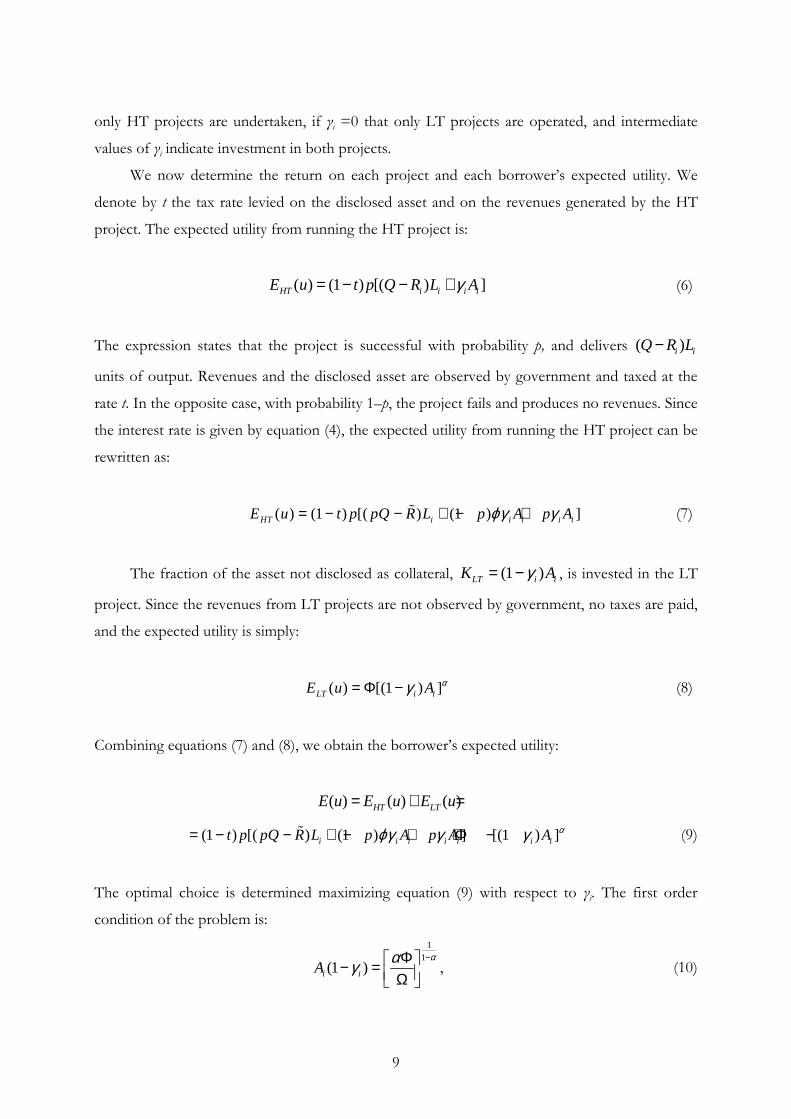
only HT projects are undertaken, if γi =0 that only LT projects are operated, and intermediate
values of γi indicate investment in both projects.
We now determine the return on each project and each borrower’s expected utility. We
denote by t the tax rate levied on the disclosed asset and on the revenues generated by the HT
project. The expected utility from running the HT project is:
( ) (1 ) [( ) ]HT i i i iE u t p Q R L Aγ= − − + (6)
The expression states that the project is successful with probability p, and delivers ( )i iQ R L−
units of output. Revenues and the disclosed asset are observed by government and taxed at the
rate t. In the opposite case, with probability 1–p, the project fails and produces no revenues. Since
the interest rate is given by equation (4), the expected utility from running the HT project can be
rewritten as:
( ) (1 ) [( ) (1 ) ]HT i i i i iE u t p pQ R L p A p Aϕγ γ= − − + − +% (7)
The fraction of the asset not disclosed as collateral, (1 )LT i iK Aγ= − , is invested in the LT
project. Since the revenues from LT projects are not observed by government, no taxes are paid,
and the expected utility is simply:
( ) [(1 ) ]LT i iE u A αγ= Φ − (8)
Combining equations (7) and (8), we obtain the borrower’s expected utility:
( ) ( ) ( )HT LTE u E u E u= + =
(1 ) [( ) (1 ) ] [(1 ) ]i i i i i i it p pQ R L p A p A A αϕγ γ γ= − − + − + + Φ −% (9)
The optimal choice is determined maximizing equation (9) with respect to γi. The first order
condition of the problem is:
11
(1 )i iAααγ
−Φ − = Ω , (10)
10
where (1 )[(1 ) ]t p pϕΩ = − − + . This condition defines the optimal γi as a function of Ai,
i.e. ( )i iAγ γ= .
It is straightforward to verify that, other things equal, a higher collateral increases
disclosure, i.e. 0i
iA
γ∂ >∂
. The result depends on the characteristics of the two projects. Borrowers
choose how much to disclose (γiAi), equating the marginal returns from the HT and LT projects.
The LT project displays decreasing returns and, hence, there is a unique level of capital
(1 )LT i iK Aγ= − that maximizes the project’s return. This implies that borrowers with higher
levels of asset endowment, Ai, will maximize returns by investing a lower share of the asset, γi, in
the LT project and, correspondingly, a higher share in the HT project whose return is a linear
function of the collateral. Hence, it could be argued that disclosure increases with the level of
assets.8
The model shows that the optimal choice of collateral and, correspondingly, the extent to
which borrowers invest in the LT project and hide their income, depends on the relative returns
from the two projects. In the next section we study how financial market development (a
reduction in the cost of credit) affects the relative return and the size of the underground
economy. We focus below on the effects of improvements in judicial efficiency, tax reforms, and
changes in the technology of underground activities.
3.3. Financial development
Financial development is a multifaceted phenomenon. It involves typically the emergence
of new and thicker capital markets, the introduction of new financial instruments, and greater
competition between intermediaries. Yet, in general, it is possible to argue that financial
development entails a lower cost of raising funds. In our model we consider financial
development as corresponding to a smaller intermediation cost δ and a lower cost of finance,
R Rδ+ ≡ % .
In this framework disclosure entails a trade-off. Disclosing collateral reduces the cost of
accessing external funding, but increases the tax burden. Furthermore, once the collateral is
8 To explain this result, recall that i LT HTA K K= + , where HT i iK Aγ≡ . Since the return on the LT project is
maximized at a given level of invested capital, [ ]1/(1 )ˆ (1 ) /LT i iK Aαγ α −≡ − = Φ Ω , any further increase in Ai will be
invested in the HT project. Hence, given ˆLT LTK K= , any increase in Ai will raise KHT and imply a higher γi.
11
disclosed, it cannot be used in the LT sector, which reduces revenues from LT projects. Financial
development reduces the size of the underground economy only if it relaxes the credit
constraints, inducing more agents to borrow. Therefore agents with very low-endowment
( miniA A< ) are not affected by financial development. To see this, recall that their expected utility
is:
( ) ( ) [(1 ) ]LT i iE u E u A αγ= = Φ − . (11)
The above expression implies that these entrepreneurs set 0iγ = . Hence, any change in the
cost of credit does not affect their investment decision. Instead, entrepreneurs whose assets are
above minA are able to access the credit market, set 1iγ < and run both projects. Moreover, for
these entrepreneurs the choice of collateral is a monotonic and increasing function of their
endowment, that is, the higher Ai, the higher γi. Figure 1 shows that the disclosure function
( )i iAγ γ= is a step function. For min0 iA A≤ < , the function coincides with the horizontal axis.
For min iA A A≤ ≤ , the function is determined by equation (10), and is therefore concave.9 Since
we assume that Ai is distributed uniformly over the interval 0,A , the area below the disclosure
function measures total disclosed assets. 10
Let us now see how financial development affects underground activities. We know from
equation (5) that a reduction in R% reduces the threshold level of collateral minA which allows
borrowers to access credit. Figure 2 shows that also a reduction in R% reduces minA to its new
value min'A . Borrowers with min min' iA A A≤ < who previously were credit constrained and
operated only in the underground economy, now disclose part of their asset, obtain a loan, and
run the HT project. The disclosure function ( )i iAγ γ= shifts accordingly: the concave portion of
the curve shifts to the right, while the section lying on the horizontal axis shrinks, as does the
activity in the formal economy. We summarize this result in the following proposition.
9 Differentiation of equation (10) shows that 0i
iA
γ∂ >∂
and ( )
2
20i
iA
γ∂ >∂
10 Entrepreneurs with assets just above Amin have two options. One is to set γi higher than the optimal value as
determined by equation (10) in order to supply enough collateral to access credit, i.e. mini iA Aγ ≥ . The alternative is
to set 0iγ = . The choice of these entrepreneurs ultimately depends on the relative return of the two technologies. It
is possible to show that there exists a threshold level of asset minA A> below which these entrepreneurs will
optimally set 0iγ = , and that above such threshold their choice is dictated by equation (10). Redefining the
threshold, however, does not change the shape of the disclosure function. Furthermore, since the threshold is a function of Amin, to simplify exposition we focus on Amin.
12
Proposition 1: Other things equal, financial development increases the opportunity cost of tax evasion, lowers
underground activity, reduces credit rationing, and stimulates investment in new technologies.
Note that in our setting financial development also implies technological improvement;
that is, more firms operate HT projects. This is in line with the empirical evidence showing that a
reduction in the size of the underground economy is associated with more efficient use of
resources and allocation of investments, see e.g. Loyaza (1996) and Farrel (2004).
A second implication of the model is that financial market development reduces credit
rationing, but can never eliminate it even in the best scenario. This depends on our assumption
that LT projects operate with decreasing returns. For low levels of assets - and, hence, for low
levels of KLT - LT projects always dominate HT projects. Using equation (10) it is easy to identify
the minimum level of asset, ALT, below which LT projects are always preferred to HT projects:
1
1
LTAαα −Φ = Ω (12)
As shown in Figure 2 all agents with 0 i LTA A≤ ≤ choose 0iγ = and run only the LT project,
regardless of the cost of financial intermediation. Thus, financial development can reduce
underground activity only if i LTA A> . The model also implies that the effect of financial
development on the size of the underground economy is non monotonic and that it is stronger at
low levels of financial development. This is because of the concavity of ( )iAγ , which measures
the amount of disclosed asset.
3.4. Judicial efficiency
As with the cost of financial intermediation, any other factor that affects the relative
returns of the two projects also affects the choice of collateral and, from equation (10), the choice
of γi. This implies that an increase in the tax rate t reduces the expected return from HT projects
and the optimal γi. For the same reasons, an increase in the productivity of LT projects (an
increase in Φ) raises the profitability of the project and reduces γi. In graphical terms, as t
increases and the expected return of HT projects falls, the disclosure function ( )iAγ shifts
downwards. This implies that each entrepreneur will disclose a lower share of assets as collateral.
13
Notice that in our model, taxation does not affect credit rationing because the tax rate does not
enter equation (5) and therefore the value of Amin.
The model also suggests that changes in judicial efficiency may affect γi. To see this, recall
that we interpret the terms (1 ) HTQθ− and (1 ) iAϕ− as the amount of resources lost in the case of
a legal dispute, and that an increase in θ or φ signals a more efficient judicial system.11 These two
parameters affect γi in two ways: (i) by reducing credit rationing, and (ii) by changing the relative
return between HT and LT projects. The first channel operates because a better judicial system
(an increase in θ or φ) reduces the threshold Amin (see equation (5)) and the region of credit
rationing. Disclosed assets increase accordingly, and the underground economy shrinks. An
increase in φ also raises the return on HT relative to LT projects. This increases also the incentive
to disclose assets and to invest in the HT technology.12
Figure 3 shows how an improvement in judicial efficiency affects γi. The increase in θ or φ
(the first channel) reduces Amin to the new value min'A . The increase in the return of HT projects
(the second channel) shifts the ( )iAγ function upwards. Hence, the new support of the disclosure
function is min[ ' , ]A A . The size of the underground economy shrinks because, in the new
equilibrium, entrepreneurs who previously were receiving credit, borrow more and disclose more
assets, while those who previously were credit rationed obtain loans and disclose part of their
assets.
Judicial efficiency also amplifies the impact of financial development on the size of the
underground economy. Figure 3 illustrates also the interaction between financial development
and judicial efficiency. An improvement in judicial efficiency shifts the disclosure function
upwards, from ( )iAγ to the new value 1( )iAγ . The thresholds minA and ALT decrease to the new
values min'A and 'LTA . Hence, financial development (a reduction of minA to min'A ) has a larger
impact on the underground economy when the judicial system is efficient. The reason is that
when the courts are efficient, financial development induces entrepreneurs to disclose a larger
fraction of their assets, so that the underground economy decreases by a larger amount.
We summarize the results of this paragraph in the following proposition:
11 In keeping with the model simplicity, we assume that it is costless to increase judicial efficiency. In general, raising judicial efficiency might require public resources and therefore a higher tax rate. However, some reforms might increase the productivity of the judicial sectors even at the same level of expenditures. For instance, Coviello et al. (2010) show theoretically and empirically that “task juggling” (the spreading of effort across too many active trials) decreases the performance of Italian judges, raising the chances of long duration of trials and exploding backlogs. Better management of judicial districts (i.e., a reduction in task juggling) would increase the productivity of judges without raising public expenditures. 12 This result can be verified by inspecting the first order condition (10).
14
Proposition 2: Other things equal, an improvement in judicial efficiency reduces the size of the underground
economy. Judicial efficiency also amplifies the impact of financial development on the size of underground economy.
3.5. The technology gap
Empirical evidence shows that the size of the underground economy differs considerably
across sectors, see Johnson et al. (2000), Batra et al. (2003) and Farrel (2004). For instance, in the
construction industry underground activities are widespread, while the chemicals and drugs
sectors are comprised mostly of formal enterprises. One of the reasons for this is due to labor
market regulation, but most of the difference depends on the technologies involved in these
sectors.
As we argue above, optimal investment and disclosure policies depend on relative returns
(and their determinants) from the available technologies. The first order condition (equation (10))
shows that a decrease in the return of LT projects (Φ) increases disclosure at each level of Ai. On
the other hand, a higher return of high tech projects (Q) does not affect investment in HT
projects directly, but reduces credit rationing by lowering Amin (see equation (5)) and reducing the
size of the underground economy. Therefore the size of the underground economy in each
sector depends on the relative returns of investment projects and the degree of credit rationing.
More dynamic and competitive sectors (e.g. the financial sector, or the chemicals industry) tend
to have higher returns (Q) from their HT projects. Firms in these sectors tend to have lower rates
of underground activities because they are less likely to be credit constrained. These sectors are
more competitive, more technologically advanced, and are likely to exhibit a lower technological
gap between HT and LT technologies. The opposite happens in less dynamic sectors (e.g.
construction or retail), where new technologies are introduced at slower rates and firms can
survive despite the implementation of mature technologies.
In our model, given the return from HT projects, the parameter Φ measures the
technological gap between the two projects. A lower Φ indicates a larger gap and therefore is
typical of less dynamic (backward) sectors while more dynamic (advanced) sectors feature a
higher Φ. As shown in Figure 4, our model predicts that the impact of financial development is
larger for backward sectors. Since Φ is lower, the disclosure function of the backward sector,
15
( )BiAγ , lies above the disclosure function of the advanced sector, ( )A
iAγ . For the same reason,
credit rationing in the backward sector is larger (which features minBA ) than in the advanced sector
( minAA ). This implies that in backward sectors the impact of financial development on the size of
the underground economy is relatively stronger. We summarize the discussion in this paragraph
in the following proposition:
Proposition 3: The size of the underground economy depends on the technological gap between LT and HT
projects. More mature and less dynamic sectors tend to display higher rates of underground activities. Other things
equal, in these sectors the impact of financial development on the underground economy is larger.
4. The data
To test the main implications of the model we use the Bank of Italy’s SHIW, which allows
us to construct an index of underground activities based on microeconomic information. SHIW
is a biannual cross-section of about 8,000 households and 24,000 individuals, and provides
detailed information on demographic variables, income, consumption, and wealth. Survey data
are available from 1977, but the main variable of interest for this paper is available only in 1995,
1998, 2000, 2002 and 2004. We exclude individuals who do not report years of contributions, are
not part of the labor force, or who work in the agricultural or public sectors. Our final sample
includes 11,781 observations.
The SHIW is a representative sample of the Italian resident population. The sample design
is similar to the Labor Force Survey conducted by ISTAT (the Italian national statistics agency).13
Data are collected through personal interviews. Questions concerning the whole household are
addressed to the family head or the person most knowledgeable about the family finances;
questions about individual incomes are answered by individual household members wherever
possible. The unit of observation is the family, which is defined to include all persons residing in
the same dwelling who are related by blood, marriage, or adoption. Individuals selected as
“partners or other common-law relationships” are also treated as families.
13 Sampling is carried out in two stages: the first covers the selection of municipalities, the second the selection of households. Municipalities are categorized into 51 strata, defined by 17 regions and 3 classes of population size (over 40,000, 20,000-40,000, less than 20,000). All municipalities in the first group are included; those in the second and third groups are selected randomly with a probability proportional to their population size. In the second stage households are selected randomly from registry office records.
16
For obvious reasons, tax evasion and underground activities are difficult to detect and
measure. Individuals and firms who evade taxes or operate irregularly tend to hide their income
from the government, and hence, are unlikely to release information on their hidden activities.
This makes it difficult to obtain direct data on underground activities and is the reason why
economists have tried different indirect measurement methods, such as the currency demand
approach, the gap between effective and potential electricity consumption, or the multiple
indicators approach.14 These methods are based on macroeconomic estimates of the size of the
underground economy, and have at least two limitations: (i) they are subject to large
measurement errors; and (ii) by construction, the resulting indicators of underground activities
are strongly correlated with other macroeconomic variables.
We overcome some of these measurement problems by constructing an index of
underground economy using microeconomic data. Of course, our survey includes no direct
questions about the extent to which each individual evades in taxes or works irregularly.
However, we can infer the degree of irregularity and evasion through the following two
questions, which are posed to each individual interviewed: (1) “How old were you when you started
working?” and “For how many years, or months, did you or your employer not pay, social security
contributions?”15
From these two questions we can construct an index of irregular activities by dividing the
number of years not covered by social security contributions by the length of the working life.
There are several advantages to using these questions. First, they are directly related to evasion of
social security contributions and irregular work, among the main signs of underground activity.
Second, while respondents are unlikely to reply to direct questions about their jobs, they may be
more inclined to report indirect information on contributions towards their pensions. Third,
since our objective is to study the relation between the underground economy and financial
development, it is straightforward to merge our index of irregular work with the index of
financial development proposed by Guiso et al. (2004), which is estimated using the same data.
Finally, and most importantly, our analysis exploits regional variability in the level of financial
development in a single country. By focusing on the same jurisdiction, we overcome the problem
14 According to this approach, a country’s shadow economy is treated as a latent variable which is then imputed using several “indicators” and “cause” variables. This method provides the widest country coverage and therefore is used extensively in the macroeconomic literature, see Djankov et al. (2002), Loyayza et al., (2005) and La Porta and Shleifer (2008). 15 The social security contribution rate is 33% of the gross wage for private and public employees and 20% in the case of self-employment.
17
that a relation between underground economy and financial development arises because both
variables are correlated with other institutional and macroeconomic indicators.
However, our indicator also has some drawbacks. As with many microeconomic variables,
an obvious source of concern is misreporting and recall bias. Another concern is that years not
covered by social contribution might be years of unemployment rather than years of irregular
work. For this reason, in our estimates we control for the local unemployment rate and per capita
GDP at the provincial level.
We also construct an alternative measure of underground economy. Following a standard
approach of the literature, we proxy underground activities by calculating the fraction of income
received in cash. The idea is that informal activities give rise to cash transactions. As our first
indicator, this variable is based on the following question available in the SHIW: Last year, did you
receive part of your (or your family) income in cash? and in which fraction? As other proxies, this indicator
has some limitations. One limitation is that it might be associated with different payment
technologies, which may themselves be related to the level of local financial development. For
this reason we use this variable only as a robustness check.
As already mentioned, the SHIW provides also an indicator of local financial development.
This indicator, proposed by Guiso et al. (2004), measures the probability that households have
access to credit, that is, that they are not credit constrained. The SHIW asks households to report
whether, in the 12 months before the interview, they have been denied credit or did not apply for
credit because they thought they would be turned down. Based on this information, and
controlling for other relevant variables, Guiso et al. (2004) estimate the probability that a
potential borrower is turned down for credit or discouraged from borrowing, controlling for a
wide range of individual and regional variables. The regional dummies obtained from the
regression model are then normalized to be equal to zero in the region with the maximum value
of the coefficient of the regional dummy (Calabria is the least financially developed region, while
March and Liguria the most developed), and therefore varies between zero and 1 (the highest
value is 0.58).
Having collected indicators of irregular activities, financial development and judicial
efficiency, we can test some of the implications of the model by estimating equations of the form:
1 2 3 4irs irs r r r s irsU X FD JUD Zα α α α µ ε= + + + + + (13)
18
where U is an indicator of irregular activities for individual i in region r and sector s, X a set of
socioeconomic indicators, FD the index of financial development, JUD a measure of judicial
inefficiency (duration of trials, described in Section 6), Z a set of regional indicators, sµ sector
fixed effects, and ε an error term. Proposition (1) suggests 1 0α < , and proposition (2) 2 0α >
(because longer length of trails is associated with less judicial efficiency and an increase of
underground activities). In the empirical section we also report separate estimates of equation
(13) by sector to verify the implication of proposition (3) that α1 and α2 should be larger in more
mature sectors.
Our analysis of the relation between financial development and the underground economy
needs to address the issue of potential reverse causality and endogeneity of financial development
FD in equation (13). In particular, an increase in underground activities (e.g. due to an increase in
general taxation) reduces the demand for credit, hampering financial market growth. Similarly,
low GDP growth might reduce the demand for loans and financial development, while at the
same time increasing underground activities. This implies that simply observing that low financial
development is associated with a high level of underground activities does not necessarily mean
that low financial development actually causes more underground activities.
In our microeconomic data, we address the endogeneity of financial development relying
on an instrument proposed by Guiso et al. (2004) which is correlated with financial development,
but is not affected by the degree of underground economy. The instrument is based on the
characteristics of the 1936 Banking Law, which over time has constrained the growth of the
Italian banking system and is an exogenous determinant of the trajectories of local financial
development. Following a period of frequent banking crises, in 1936 Italian legislators attempted
to stabilize the financial system by strictly limiting in each region the number of banks and bank
branches. In achieving this aim, the law has worked very well, as witnessed by the fact that the
number of new branches in Italy after 1936 has expanded very little. Yet, in some regions and for
some local credit institutions (such as savings banks and cooperative banks) the 1936 Banking
Law has been less constraining. Therefore the 1936 Law explains a large part of the variability in
local financial development even after 60 years. Guiso et al. (2004) test this hypothesis by
estimating the correlation between the index of regional financial development and the
characteristics of the banking system before the 1936 Law. They find that 1936 bank branches,
local branches, saving banks and cooperative banks (each in per capita terms) explain 72% of the
regional variation in credit supply in the 1990s. In our empirical estimates we use the same
19
instruments which is uncorrelated to underground economy to control for endogeneity in
financial development.
5. Descriptive analysis
Our microeconomic indicator of irregular activities is consistent with macroeconomic
estimates from different sources. Figure 5 plots the regional averages of the index of job
irregularity against a similar index, produced by ISTAT but based on the Labor Force Survey.
Despite the very different methods of elicitation, a strong correlation between the two measures
is evident (the correlation coefficient is 0.87). Both indicators show that Southern regions feature
the highest levels of underground economy. In particular, in Campania, Sicily, Sardinia, and other
Southern regions the irregular job rate exceeds 30%, more than twice as high as the level of
irregularity in Northern regions such as Friuli and Emilia-Romagna. The South is also much less
developed in terms of per capita GDP, infrastructure, and human capital. It is characterized by
more corruption, less efficient government, and higher levels of organized crime. Each of these
factors potentially contributes to generating a large underground economy. Yet these regions also
display relatively low levels of financial development, and we argue that this channel plays an
important role in shaping the underground economy.
Figure 6 plots the relation between financial development and the size of the underground
economy. We use regional averages for the period 1995-2004. The correlation is strongly negative
(-0.81) and statistically different from zero at the 1% level. Figure 6 shows a strong geographical
divide. For example, in Campania a high irregular job rate (36%) is coupled with an index of
financial development of only 3%. In contrast, Lombardy (the richest region in the North) has a
much lower irregular job rate (16%) but a much higher index of financial development (43%).
In Italy, as in many other countries, there are significant differences by sector in the level of
underground activity. The index of job irregularity reaches 30.8% in the construction sector, 25%
in the retail and tourism sectors, but is much lower (12% and 15% respectively) in the financial
and manufacturing sectors. These differences clearly reflect structural and technological
differences between sectors. Underground activities are more widespread in low value added
sectors with relatively low competition and smaller firm sizes. Note that this is one of the
predictions of the model, because firms operating in more mature sectors have fewer incentives
to invest and lower opportunity costs of hiding revenue.
20
Descriptive statistics show also that the size of the underground economy depends on the
nature of employment. Self-employed, professionals, and entrepreneurs are much more likely to
work in the underground economy (the index of job irregularity in these occupations ranges from
24% for self-employed to 26% for professionals and entrepreneurs). For managers (8%), and
clerks (12%) irregular activities are much less widespread. One reason for this is that, in Italy,
employers deduct the tax before transferring wages to employees. This implies that it is much
more difficult for employees to evade taxes and social contributions. Therefore hidden activities
arise from extra work not supported by a formal employment contract. In the next section we
present regressions for the relation between local financial development and the underground
economy, controlling for possible sources of endogeneity and other factors (such as sector and
occupation) which might influence the relationship.
6. Regression evidence
In our empirical estimates we regress the irregular job rate on the indicator of local
financial development and a set of individual variables (gender, age, years of education, marital
status, disposable income). Each regression also includes time dummies; some of the
specifications include occupation or/and sector dummies. We also include an indicator to control
for judicial inefficiency, using ISTAT data. This indicator measures the length of ordinary civil
trials, that is, the time elapsing from the date of the initial recording of a trial to the sentence, for
actions requiring adjudication of substantive rights concerning credit and commercial matters
such as loans, sale of real estate or goods, rentals, negotiable and quasi-negotiable instruments,
and insurance.16 The enforcement cost is directly related to the length of the judicial process. A
long trial increases the legal expenses and, for disputed loans, the interest income that is forgone
when the collateral does not cover the judicial costs. Moreover, during the time of the trial, the
creditor is exposed to the danger of asset substitution by the debtor and to unexpected changes
in the value of collateral. Therefore we expect that judicial inefficiency is associated with more
underground activities (α2>0 in equation (13)).
16 A narrower classification of legal action (e.g., loans only) produces too few observations for each district-year cell to compute reliable indicators of judicial inefficiency. For the same reason we do not consider the length of appeals in civil cases and bankruptcy procedures.
21
We start our analysis by presenting the OLS regressions. Since some of the right-hand side
variables vary only between provinces or regions (judicial inefficiency, local unemployment rate,
financial market development), standard errors are adjusted for clustering at the provincial level.
Table 2, column 1 presents our baseline model. The demographic variables explain a substantial
part of the variability of the irregular job rate. In particular, we find that women and younger
individuals with lower levels of education are more likely to work irregularly, while higher
disposable income increases the likelihood of operating in the formal sector.
The main variable of interest is financial development. The coefficient of this variable is
negative and statistically different from zero at the 1% level, which is consistent with the model’s
prediction (α1<0 in equation (13)). Its impact is sizable: raising financial development by 10
percentage points (approximately the distance between Tuscany and Emilia-Romagna) reduces
the irregular job rate by 2.2 percentage points. Lower judicial efficiency is associated with a higher
rate of irregular working (the coefficient is 0.083 and is statistically different from zero at the 1%
level). Note that the model in Section 2 suggests that judicial efficiency may affect the size of the
underground economy both directly and indirectly. Directly, judicial efficiency reduces the size of
the underground economy by increasing the opportunity cost of hiding income. Indirectly, an
improvement in judicial efficiency increases the value of collateral and reduces the cost of credit.
Therefore, the effect of judicial efficiency is captured partly by the index of local financial
development.
In Table 2, column 2 we add to the baseline model a dummy for the South and an indicator
of social capital (fraction of the population participating in general elections in each province).17
The coefficients of both variables are positive, but only the dummy for the South is statistically
different from zero. Since Southern regions tend also to be the least financially developed and
feature the highest judicial inefficiency, introducing this dummy attenuates the impact of financial
development (coefficient is -0.184) and judicial inefficiency (0.038). Furthermore, while the
coefficient of financial development is still statistically different from zero at the 1% level, the
effect of judicial inefficiency is now less precisely estimated than in the regression in column 1.
The third specification in Table 2 repeats the estimation introducing sector and occupation
dummies, and the results are essentially unaffected. The final specification in Table 2, column 4
adds the provincial unemployment rate to control for the fact that some of the irregular work
might be due to spells of unemployment. The coefficient of this indicator is not statistically
different from zero, and again the other coefficients are unaffected. Other regressions with
17 Other common proxies for social capital (e.g., non profit organizations) deliver qualitatively similar results.
22
indicators of local labor markets conditions (such as provincial GDP per capita) and other
regional or provincial variables (e.g. crime rates) provide similar results.
The impact of financial development on the level of the underground economy is sizable.
Using the coefficients of column 2 in Table 2, we calculate the impact in a scenario in which
financial development in each region is raised to the standards of the most developed region
(Marche). The results are plotted in Figure 7, and indicate that in this hypothetical scenario the
reduction in the underground economy is quite sizable in Calabria and Campania (10%),
intermediate in Tuscany and Sardinia (4%), and lowest in the most financially developed regions
(Emilia and Liguria).
Table 3 probes further in our results presenting two robustness checks. We re-estimate the
model defining the number of working years used to compute the irregular job rate as the
difference between current age and age when completed education. This measure is not subject
to recall bias on the part of respondents and provides therefore a more objective measure of
number of working years.18 The new variable is not identical, but strongly correlated with the
irregular job rate as previously calculated (the correlation coefficient is 0.83). The regressions
results are reported in the first two columns of Table 3. All regressions coefficients are similar in
size and significance to those reported in columns 3 and 4 of Table 2.
We also present regressions using our second proxy for the underground economy, i.e. the
fraction of income received in cash. The results are reported in columns 3 and 4 of Table 3. The
results are again aligned to those of Table 2. It is remarkable that the coefficients of financial
development (-0.194 and -0.216) are quite similar to those obtained using the irregular job rate as
the dependent variable in columns 3 and 4 of Table 2 (-0.189 and -0.186, respectively).
The next step is to tackle the issue of the potential endogeneity of financial development.
In Table 4 we repeat the estimation using the same instruments as in Guiso et al. (2004): number
of branches per capita in 1936, number of local branches in 1936, number of saving banks per
capita in 1936, and number of cooperative banks per capita in 1936. These variable pass standard
tests of validity of the instruments.19 The IV regressions confirm the OLS results. Financial
development negatively and significantly affects the level of the underground economy, and the
results are robust under the different specifications. With the exception of the regression in
column 1, the coefficient sizes are quite similar to those in the regressions in Table 2.
18 We thank an anonymous referee for this suggestion. 19 The F-test on the first-stage instruments reported in Table 4 indicates that the instruments are significant predictors of financial development. The Sargan test does not reject the hypothesis that the excluded instruments are valid. Except for the regression in column 1, the Wooldridge's (1995) robust score test does not reject the hypothesis that the variables are exogenous.
23
The mechanism behind our theoretical model is that firms have an incentive to move from
low return technologies (LT projects) to more innovative technologies (HT projects). This shift
in production occurs through credit markets, pledging more resources, and emerging into the
formal sector. Technological gaps between LT and HT projects therefore are crucial for shaping
the incentives to operate in the formal economy or in the underground sector. Since these gaps
depend on the specificity of the production process, we want to check whether the effect of
financial development is disproportionate in some sectors. We are especially interested in testing
the prediction of the model that in mature sectors the impact of financial development on the
underground economy is larger than in more dynamic sectors.
Tables 5 and 6 respectively present the OLS and IV regressions by sector. Figure 7 showed
that the underground economy is much more widespread in the construction, retail, and
transportation sectors. Our regression estimates show that it is precisely in these sectors that
financial development has the strongest negative impact on the irregular job rate, regardless of
the estimation method. In particular, in the OLS regressions the coefficient of financial
development is -0.353 for the construction sector, -0.287 for retail and tourism and -0.198 for
transportation, as opposed to -0.076 and -0.131 in the financial and manufacturing sectors,
respectively. The other coefficients are broadly in line with the full sample estimates. Higher
education and higher disposable income are generally associated with a lower rate of irregularity.
The coefficients of the South dummy and of the indicator of judicial inefficiency are generally
positive, but statistically different from zero only in the regressions for the financial sector (the
dummy for South is also significant in the regressions for manufacturing). As in the full sample
estimates, the IV estimates pass the standard tests of validity of instruments (except for the
exogeneity test in the financial and real estate sectors).
7. Conclusions
The existence of a large underground economy represents a relevant burden on society.
The underground economy can slow the investment rate, reduce the adoption of new
technologies, and limit the ability of governments to raise sufficient resources to pay for public
goods and for infrastructure. Eventually, it can affect the allocation of real resources and thwart
economic growth. A high level of taxation, cumbersome and inefficient bureaucracy, and poor
legal protection are among the factors that have been identified as the major causes of tax
24
evasion and a large underground economy. In this paper we focus on financial development, a
factor that has received less attention from economists.
The main idea is that when individuals and firms hide all or part of their income, they pay
less taxes, but they also face a higher cost of credit. Therefore, the choice of operating in the
underground economy involves a trade-off. By reducing the cost of credit or by granting credit to
previously credit constrained agents, financial development affects the trade-off, increasing the
incentive to operate in the formal economy. We capture these ideas in a simple model in which
agents choose to disclose their collateral in order to obtain credit for investment in a high-return
project. The alternative is to operate in the informal sector in a low-return project using only
internal funds. The choice to go underground therefore is also a choice between different
technologies. The model predicts that financial development (a reduction in the cost of credit)
induces firms to disclose more assets and to invest in a high-tech project, and that this effect is
stronger in mature sectors. Furthermore, an improvement in judicial efficiency reduces the cost
of credit and the size of the underground economy.
In the second part of the paper we test the main implications of the model using Italian
microeconomic data. We build an index of job irregularity using the 1995-2004 Bank of Italy
SHIW, and regress this index on an indicator of local financial development, judicial inefficiency,
and other individual and regional variables. The results show that the underground economy is
strongly negatively correlated with financial development, even when we control for financial
development endogeneity. We find also that more competitive and innovative sectors display a
lower level of underground activity, and that financial development has a stronger impact in
mature sectors (such as construction, retail, tourism). The effect of judicial inefficiency is in line
with the model’s predictions, but the coefficient is not statistically different from zero if we
control for other regional variables.
Our study implies that successful programs to reduce the extent of the underground
economy should take into account the structure of credit markets, and implies also that financial
market development has important spillover effects. By reducing the incentives to operate in the
underground economy, financial market development can stimulate the adoption of new
technologies, reduce the size of the underground economy, and increase tax collection levels.
25
References
Antunes, A. R. and Cavalcanti, T. V. D. V. (2007), "Start Up Costs, Limited Enforcement, and the Hidden Economy", European Economic Review, Vol. 51, pp. 203-224.
Arthur, W. B. (1989), "Competing Technologies, Increasing Returns, and Lock-in by Historical Events", The Economic Journal, Vol. 99, pp. 116-131.
Batra, G., Kaufmann, D. and Stone, A. H. (2003), "The Firms Speak: What the World Business Environment Survey Tells Us about Constraints on Private Sector Development", World Bank Working Paper.
Battisti, G. and Stoneman, P. (2003), "Inter-and Intra-Firm Effects in the Diffusion of New Process Technology", Research Policy, Vol. 32, pp. 1641-1655.
Battisti, G. and Stoneman, P. (2005), "The Intra-Firm Diffusion of New Process Technologies", International Journal of Industrial Organization, Vol. 23, pp. 1-22.
Beck, T., Lin, C. and Ma, Y. (2010), "Why Do Firms Evade Taxes? The Role of Information Sharing and Financial Sector Outreach", European Banking Center Discussion Paper n. 26.
Blackburn, K., Bose, N. and Capasso, S. (2012), "Tax Evasion, the Underground Economy and Financial Development", Journal of Economic Behavior and Organization, Vol. 83, pp. 243-253.
Bose, N., Capasso, S. and Wurm, M. (2008), "The Impact of Banking Development on the Size of the Shadow Economy", CSEF Working Papers No. 207.
Capasso, S. and Mavrotas, G. (2010), "Loan Processing Costs, Information Asymmetries and the Speed of Technology Adoption", Economic Modelling, Vol. 27, pp. 358-367.
Cerqueti, R. and Coppier, R. (2011), "Economic Growth, Corruption and Tax Evasion", Economic Modelling, Vol. 28, pp. 489-500.
Coviello, D., Ichino, A., and Persico, N. (2010), "Don't Spread Yourself Too Thin: The Impact of Task Juggling on Workers' Speed of Job Completion," NBER Working Paper No. 16502.
Dabla-Norris, E. and Feltenstein, A. (2005), "The Underground Economy and Its Macroeconomic Consequences", Journal of Policy Reform, Vol. 8, pp. 153-174.
Dabla-Norris, E., Gradstein, M. and Inchauste, G. (2008), "What Causes Firms to Hide Output? The Determinants of Informality", Journal of Development Economics, Vol. 85, pp. 1-27.
Djankov, S., La Porta, R., Lopez-De-Silanes, F. and Shleifer, A. (2002), "The Regulation of Entry", Quarterly Journal of Economics, Vol. 117, pp. 1-37.
Dreher, A., Kotsogiannis, C. and Mccorriston, S. (2009), "How do Institutions Affect Corruption and the Shadow Economy?" International Tax and Public Finance, Vol. 16, pp. 773-796.
Dreher, A. and Schneider, F. (2010), "Corruption and the Shadow Economy: An Empirical Analysis", Public Choice, Vol. 144, pp. 215-238.
Ellul, A., T. Jappelli, M. Pagano & F. Panunzi (2012), "Transparency, Tax Pressure and Access to Finance," CEPR Discussion Papers 8939.
Farrel, D. (2004), "The Hidden Dangers of the Informal Economy", The McKinsey Quarterly, Vol. 3.
26
Feld, L. P. and Schneider, F. (2010), "Survey on the Shadow Economy and Undeclared Earnings in OECD Countries", German Economic Review, Vol. 11, pp. 109-149.
Frey, B. S. and Torgler, B. (2007), "Tax Morale and Conditional Cooperation", Journal of Comparative Economics, Vol. 35, pp. 136-159.
Friedman, E., Johnson, S., Kaufmann, D. and Zoido-Lobaton, P. (2000), "Dodging the Grabbing Hand: The Determinants of Unofficial Activity in 69 Countries", Journal of Public Economics, Vol. 76, pp. 459-493.
Gatti, R. and Honorati, M. (2008), "Informality among Formal Firms: Firm-Level, Cross-Country Evidence on Tax Compliance and Access to Credit", World Bank Policy Research Working Paper N. 4476.
Guiso, L., Sapienza, P. and Zingales, L. (2004), "Does Local Financial Development Matter?" Quarterly Journal of Economics, Vol. 119, pp. 929-969.
Hollenstein, H. and Woerter, M. (2008), "Inter-and Intra-Firm Diffusion of Technology: The Example of E-commerce: An Analysis Based on Swiss Firm-Level Data", Research Policy, Vol. 37, pp. 545-564.
Jappelli, T., Pagano, M. and Bianco, M. (2005), "Courts and Banks: Effects of Judicial Enforcement on Credit Markets", Journal of Money, Credit and Banking, Vol. 37, pp. 223-244.
Johnson, S., Kaufmann, D. and Zoido-Lobaton, P. (1998a), "Regulatory Discretion and the Unofficial Economy", The American Economic Review, Vol. 88, pp. 387-392.
Johnson, S., Kaufmann, D. and Zoido-Lobatón, P. (1998b), "Corruption, Public Finance, and the Unofficial Economy", World Bank Discussion Papers.
Johnson, S., Kaufmann, D., Mcmillan, J. and Woodruff, C. (2000), "Why Do Firms Hide? Bribes and Unofficial Activity after Communism", Journal of Public Economics, Vol. 76, pp. 495-520.
La Porta, R. and Shleifer, A. (2008), "The Unofficial Economy and Economic Development", NBER Working Paper No. 14520.
Loayza, N. V. (1996), "The Economics of the Informal Sector: A Simple Model and Some Empirical Evidence from Latin America", Carnegie-Rochester Conference Series on Public Policy, Vol. 45, pp. 129-162.
Loayza, N., Oviedo, A. and Serven, L. (2005), "The Impact of Regulation on Growth and Informality: Cross-Country Evidence", World Bank Policy Research Working Paper No. 3623.
Mansfield, E. (1963), "Intra-Firm Rates of Diffusion of an Innovation", The Review of Economics and Statistics, Vol. 45, pp. 348-359.
Pant, M., Chowdhury, P. R. and Singh, G. (2009), "Financial intermediation and employment", Review of Market Integration, Vol. 1, pp. 61-82.
Rosenberg, N. (1982) Inside the Black Box: Technology and Economics. Cambridge: Cambridge University Press.
Schneider, F. (2005), "Shadow Economies Around the World: What Do We Really Know?" European Journal of Political Economy, Vol. 21, pp. 598-642.
27
Schneider, F. (2007), "Shadow Economies and Corruption all Over the World: New Estimates for 145 Countries", Economics: The Open-Access, Open-Assessment E-Journal, Vol. 1, pp. 2007-2009.
Schneider, F. (2010), "The Influence of Public Institutions on the Shadow Economy: An Empirical Investigation for OECD Countries", Review of Law and Economics, Vol. 6, pp. 113-140.
Schneider, F. and Enste, D. H. (2000), "Shadow Economies: Size, Causes, and Consequences", Journal of Economic Literature, Vol. 38, pp. 77-114.
Straub, S. (2005), "Informal Sector: The Credit Market Channel", Journal of Development Economics, Vol. 78, pp. 299-321.
Teobaldelli, D. (2011), "Federalism and the Shadow Economy", Public Choice, Vol. 146, pp. 269-289.
Torgler, B., Schneider, F. and Schaltegger, C. A. (2010), "Local Autonomy, Tax Morale, and the Shadow Economy", Public Choice, Vol. 144, pp. 293-321.
28
Figure 1
The disclosure function
Figure 2
The effect of financial development on the underground economy
γi
Ai ALT
MinA A
γi =1
γi
Ai LTA MinA A 'MinA
γi =1
29
Figure 3
The effect of judicial efficiency on the underground economy
Figure 4 The effect of financial development in advanced and mature sectors
Ai
γi
'LTA MinA A 'MinA LTA
γi =1
1( )iAγ
( )iAγ
γi
Ai ALTA A B
LTA
( )A iAγ
( )B iAγ
minAA min
BA
1γ =
30
Figure 5
Irregular job rate: Comparison between ISTAT and SHIW
Abruzzo
Basilicata
Calabria
Campania
Emilia
Friuli
Lazio
LiguriaLombardia
Marche
Molise
Piemonte
Puglia
Sardegna
Sicilia
Toscana
Trentino Umbria
Veneto
.1.2
.3.4
.1 .15 .2 .25 .3
Irre
gula
r jo
b ra
te, S
HIW
Irregular job rate, ISTAT
Figure 6 Irregular job rate and financial development
Abruzzo
Basilicata
Calabria
Campania
Emilia
Friuli
Lazio
LiguriaLombardia
Marche
Molise
Piemonte
Puglia
Sardegna
Sicilia
Toscana
TrentinoUmbria
Veneto
.1.1
5.2
.25
.3.3
5
0 .2 .4 .6
Irre
gula
r jo
b ra
te
Financial development
31
Figure 7
Financial development and the underground economy – Raising financial development to the standards of the most developed region
-.1 -.05 0
Marche
Liguria
Emilia
Veneto
Piemonte
Trentino
Lombardia
Friuli
Umbria
Sardegna
Toscana
Abruzzo
Basilicata
Molise
Sicilia
Puglia
Lazio
Campania
Calabria
Reduction in irregular job rate (based on estimates of column 4 in Table 2)
32
Table 1
Descriptive statistics
Variable Mean Median Standard deviation
Irregular job rate 0.2038 0.0870 0.2735 Fraction of income received in cash 0.3100 0.0000 3999 Financial development 0.3689 0.4350 0.1753 Male 0.8523 1.0000 0.3548 Age 44.0546 44.0000 9.7390 Education 3.4128 3.0000 0.8801 Married 0.8041 1.0000 0.3969 Log disposable income 10.3357 10.3482 0.6222 Judicial inefficiency 1.2315 1.1494 0.2494 Social capital 0.8144 0.8378 0.0803 South 0.2401 0.0000 0.4271 Provincial unemployment rate 0.1078 0.0847 0.0684 Manufacturing 0.3988 0.0000 0.4897 Construction 0.1280 0.0000 0.3341 Retail and tourism 0.2414 0.0000 0.4280 Transportation 0.0766 0.0000 0.2659 Financial and real estate 0.1552 0.0000 0.3621 Operative 0.3770 0.0000 0.4846 Clerk 0.1985 0.0000 0.3989 Manager 0.0748 0.0000 0.2632 Professional 0.0722 0.0000 0.2588 Entrepreneur 0.0287 0.0000 0.1670 Self-employed 0.3770 0.0000 0.4846
Note. Data are drawn from the 1995-2004 SHIW. Sample statistics refer to the pooled sample of 11781 observations.
33
Table 2 Financial development and the underground economy - OLS regressions
(1)
(2) (3) (4)
Financial development -0.223 -0.184 -0.189 -0.186 (0.037)*** (0.058)*** (0.056)*** (0.055)*** Male -0.034 -0.035 -0.043 -0.044 (0.012)*** (0.012)*** (0.012)*** (0.012)*** Age -0.022 -0.022 -0.020 -0.020 (0.003)*** (0.003)*** (0.003)*** (0.003)*** Age square 0.000 0.000 0.000 0.000 (0.000)*** (0.000)*** (0.000)*** (0.000)*** Years of education -0.020 -0.020 -0.017 -0.017 (0.007)*** (0.007)*** (0.008)** (0.008)** Married -0.026 -0.030 -0.024 -0.023 (0.009)*** (0.009)*** (0.009)*** (0.009)** Log disposable income -0.079 -0.076 -0.075 -0.075 (0.008)*** (0.008)*** (0.008)*** (0.008)*** Judicial inefficiency 0.083 0.038 0.014 0.007 (0.026)*** (0.028) (0.031) (0.038) Social capital 0.093 0.069 0.085 (0.127) (0.130) (0.149) South 0.069 0.059 0.053 (0.023)*** (0.022)** (0.024)** Provincial unemployment rate 0.085 (0.215) Constant 1.606 1.518 1.584 1.582 (0.121)*** (0.145)*** (0.179)*** (0.187)*** Year dummies YES YES YES YES Sector dummies NO NO YES YES Occupation dummies NO NO YES YES Observations 11781 11781 11779 11673 R-squared 0.12 0.13 0.17 0.17
Note. The sample refers to the 1995-2004 SHIW. Standard errors, adjusted for clustering at the provincial level, are reported in parenthesis. * significant at the 10% level, ** significant at the 5% level, *** significant at the 1% level.
34
Table 3 Financial development and the underground economy – robustness checks
Irregular job rate Fraction of income received in cash
Note. In columns (1) and (2) the definition of irregular job rate is based on the difference between age and the age when completed education. In columns (3) and (4) the dependent variable is the fraction of income received in cash. The sample refers to the 1995-2004 SHIW. Standard errors, adjusted for clustering at the provincial level, are reported in parenthesis. * significant at the 10% level, ** significant at the 5% level, *** significant at the 1% level
35
Table 4 Financial development and the underground economy. IV regressions
(1)
(2) (3) (4)
Financial development -0.311 -0.179 -0.187 -0.189 (0.050)*** (0.059)*** (0.056)*** (0.055)*** Male -0.036 -0.034 -0.043 -0.044 (0.012)*** (0.012)*** (0.012)*** (0.012)*** Age -0.022 -0.021 -0.020 -0.020 (0.003)*** (0.003)*** (0.003)*** (0.003)*** Age square 0.000 0.000 0.000 0.000 (0.000)*** (0.000)*** (0.000)*** (0.000)*** Years of education -0.020 -0.020 -0.017 -0.017 (0.007)*** (0.007)*** (0.008)** (0.008)** Married -0.027 -0.030 -0.024 -0.023 (0.009)*** (0.009)*** (0.009)*** (0.009)** Log disposable income -0.077 -0.076 -0.075 -0.075 (0.008)*** (0.008)*** (0.008)*** (0.008)*** Judicial inefficiency 0.043 0.039 0.014 0.007 (0.031) (0.028) (0.030) (0.037) Social capital 0.090 0.067 0.086 (0.128) (0.132) (0.149) South 0.070 0.059 0.053 (0.023)*** (0.022)*** (0.024)** Provincial unemployment rate 0.082 (0.216) Constant 1.672 1.518 1.592 1.575 (0.124)*** (0.144)*** (0.175)*** (0.187)*** Year dummies YES YES YES YES Sector dummies NO NO YES YES Occupation dummies NO NO YES YES Observations 11781 11781 11779 11673 F-test on first-stage instruments 29.91 47.01 47.35 70.50 Test of over-identifying restrictions (p-value) 0.54 0.78 0.66 0.42 Exogeneity test (p-value) 0.02 0.78 0.90 0.87
Note. The sample refers to the 1995-2004 SHIW. The instruments are: branches per capita in 1936, local branches in 1936, number of saving banks per capita in 1936, and number of cooperative banks per capita in 1936. Standard errors, adjusted for clustering at the provincial level, are reported in parenthesis. * significant at the 10% level, ** significant at the 5% level, *** significant at the 1% level.
36
Table 5 Financial development and the underground economy, by sector. OLS regressions
Note. The sample refers to the 1995-2004 SHIW. Standard errors, adjusted for clustering at the provincial level, are reported in parenthesis. * significant at the 10% level, ** significant at the 5% level, *** significant at the 1% level.
37
Table 6 Financial development and the underground economy, by sector. IV regressions
Note. The sample refers to the 1995-2004 SHIW. The instruments are: branches per capita in 1936, local branches in 1936, number of saving banks per capita in 1936, and number of cooperative banks per capita in 1936. Standard errors, adjusted for clustering at the provincial level, are reported in parenthesis. * significant at the 10% level, ** significant at the 5% level, *** significant at the 1% level.