Financial Feasibility Assessments Building and Using Assessment Models for Financial Feasibility Analysis of Investment Projects Anna Regína Björnsdóttir Faculty of Industrial Engineering, Mechanical Engineering and Computer Science University of Iceland 2010
Transcript
Financial Feasibility Assessments
Building and Using Assessment Models for Financial Feasibility Analysis of Investment Projects
Anna Regína Björnsdóttir
Faculty of Industrial Engineering, Mechanical Engineering and Computer Science
University of Iceland 2010
Financial Feasibility Assessments
Building and Using Assessment Models for Financial Feasibility Analysis of Investment Projects
Anna Regína Björnsdóttir
60 ECTS thesis submitted in partial fulfillment of a Magister Scientiarum degree in Industrial Engineering
Advisors Dr. Páll Jensson
Þorbjörg Sæmundsdóttir
Faculty Representative Dr. Helgi Þór Ingason
Faculty of Industrial Engineering, Mechanical Engineering and Computer Science
School of Engineering and Natural Sciences University of Iceland
Abstract This thesis examines how assessment models can be built and used for financial feasibility analysis of investment projects. An overview of financial feasibility assessment methods is presented, as well as a general assessment model, which can be used as a base when constructing new models. Risk analysis methods are introduced, as uncertainties can highly affect the outcome of the assessment. A new optimization method used to estimate financing requirements of investment projects is presented, as well as a new method to predict the optimal year to sell the investment. A case study is used to illustrate the use of a model to assess the financial feasibility of a geothermal cogeneration plant. The conclusion is that Net Present Value, Internal Rate of Return and Modified Internal Rate of Return should be used to assess financial feasibility of investment projects. In addition to calculating the financial feasibility criteria, assessment models should allow the user to perform sensitivity analysis, scenario analysis, and simulation to analyze risk associated with the investment project.
Útdráttur Þessi ritgerð fjallar um smíði og notkun líkana við greiningu á arðsemi fjárfestingarverkefna. Arðsemisgreiningaraðferðir eru dregnar saman í ritgerðinni og almennt arðsemislíkan, sem nota má sem grunn að nýjum líkönum, sett fram. Aðferðir við áhættugreiningu er kynntar, þar sem óvissa getur haft mikil áhrif á niðurstöður arðsemismatsins. Ný bestunaraðferð til að finna fjármögnunarþörf verkefna er kynnt, ásamt nýrri aðferð til að spá fyrir um á hvaða ári sé hagstæðast að selja fjárfestinguna. Bygging jarðvarmavirkjunar er notuð sem rannsóknardæmi til að sýna hvernig hægt sé að nota líkan til að meta arðsemi verkefnis. Niðurstaða verkefnisins er sú að nota ætti núvirði, innri vexti og leiðrétta innri vexti til að meta arðsemi fjárfestingarverkefna. Auk útreikninga á arðsemimælikvörðum ættu arðsemislíkön að gefa kost á að nota næmnigreiningu, sviðsmyndagreiningu og hermun til að greina áhættu tengda fjárfestingarverkefninu.
Table of Contents List of Figures .................................................................................................................... ix
List of Tables ...................................................................................................................... x
Acknowledgements .......................................................................................................... xi
4 Case Study – A Geothermal Power Plant ............................................................... 31 4.1 Geothermal Energy Utilization ........................................................................ 31 4.2 The Model ............................................................................................................ 33
4.2.1 Model Inputs and Assumptions ............................................................. 34 4.2.2 Model Calculations ................................................................................... 39 4.2.3 Model Results ............................................................................................ 40
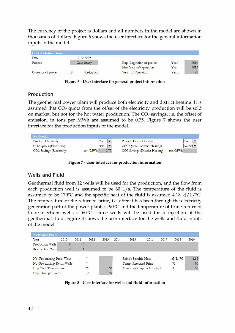
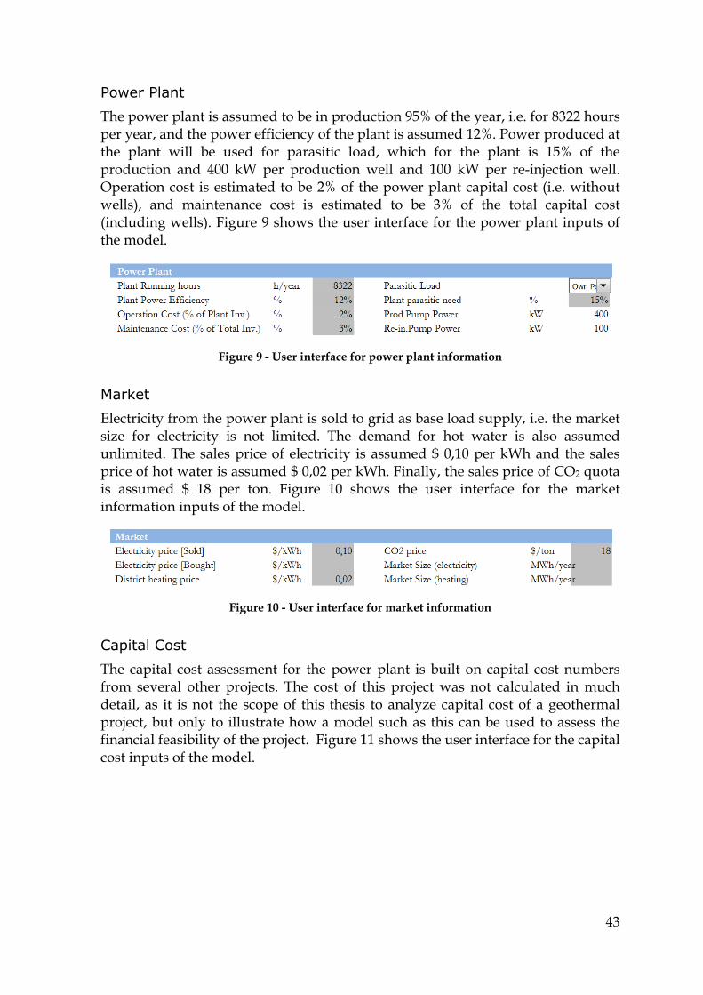
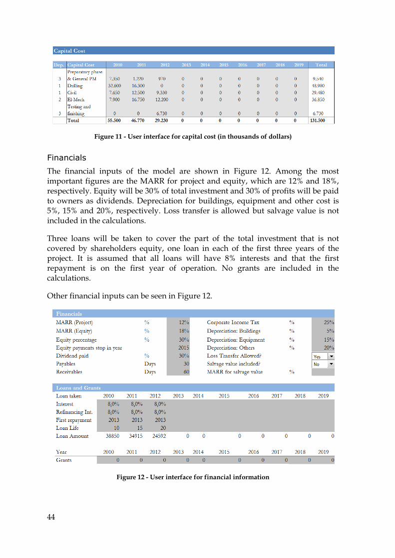
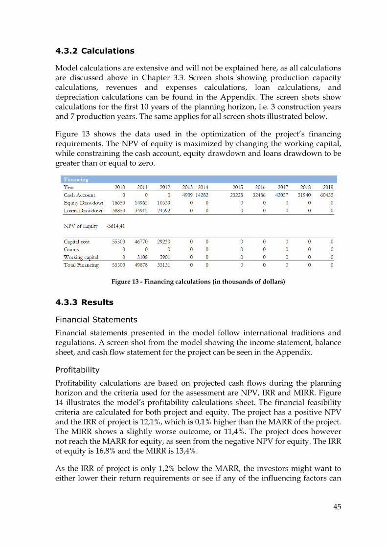
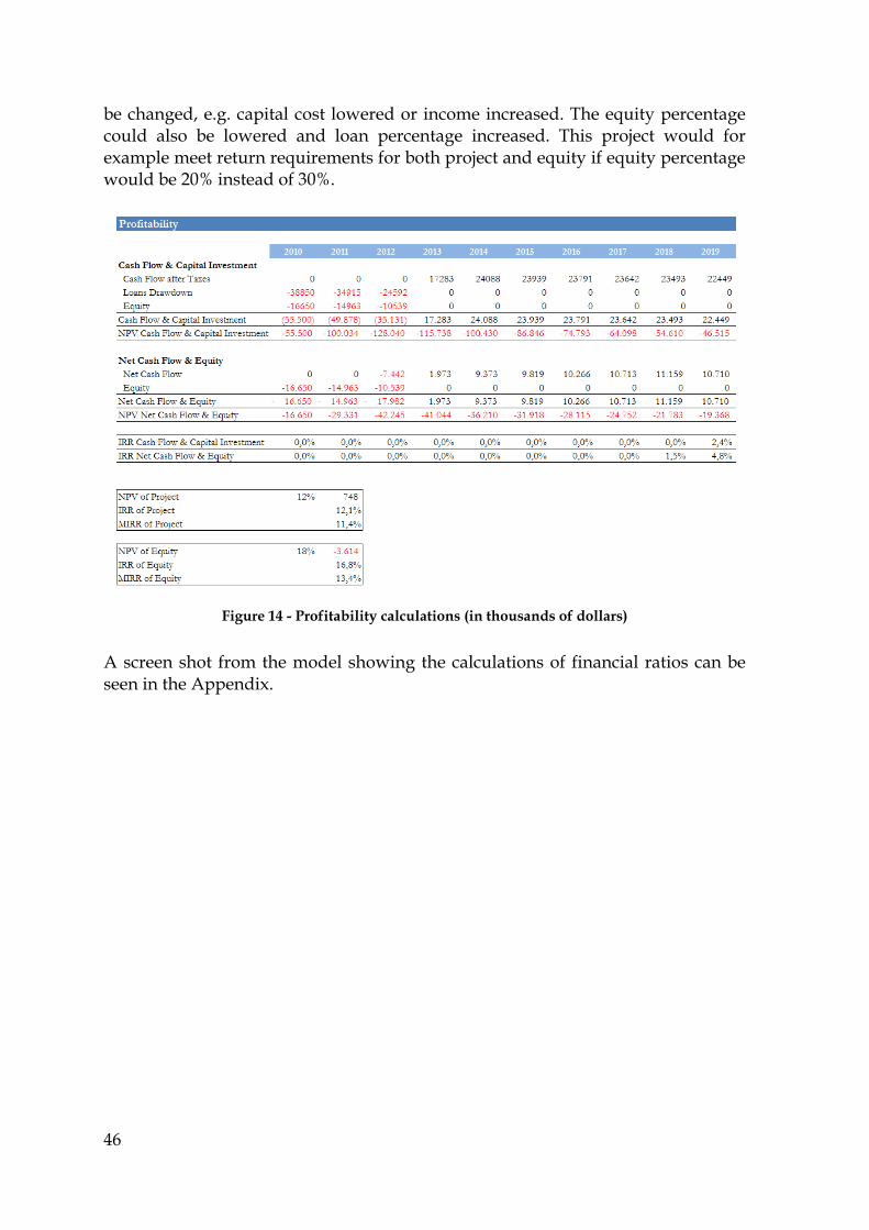
4.3 Case Study ........................................................................................................... 41 4.3.1 Inputs and Assumptions .......................................................................... 41 4.3.2 Calculations ............................................................................................... 45 4.3.3 Results ......................................................................................................... 45
List of Tables Table 1 - Scenario summary for case study project ..................................................... 56
xi
Acknowledgements First of all I would like to express my gratitude to my advisors, Dr. Páll Jensson for his academic guidance and support, and Þorbjörg Sæmundsdóttir for all the constructive criticism, and her endless patience and support.
I would also like to thank Dr. Páll Valdimarsson, Kristín Vala Matthíasdóttir and Lilja Tryggvadóttir for explaining technical details to me and for answering all my questions on geothermal energy.
Finally, I would like to express my love and gratitude to my family for their support, patience and help during the course of this work.
1
1 Introduction Before an investment decision is made it is necessary to determine whether or not the planned investment idea is feasible. The feasibility of an investment has to be considered with respect to several different aspects in order to determine whether the investment should be realized or not. Carrying out a feasibility analysis is therefore one of the most critical steps in the decision-making process.
A feasibility analysis is an effective analytical tool that can be used to evaluate investments from various perspectives, e.g. technical, social, legal, financial, market, and organizational. Financial feasibility is often a predominant factor in feasibility analysis, as most investments are not realized if they do not generate profit for the project owners. The focus of this thesis is on financial feasibility analysis and its application in the decision-making process.
Precision and reliability of financial feasibility analysis relies on the accuracy of information used in the analysis. The appropriate level of detail has to be decided with respect to what stage the investment is on. On early stages the level of uncertainty is often high, but as the investment opportunity evolves information become more detailed and reliable. As uncertainty can highly affect the results of the analysis, the level of detail has to be taken into account when basing decisions on the results.
To assess the financial feasibility of investments relevant criteria have to be chosen. Financial feasibility calculations need to be done with care and the complexity of the calculations depends on the number of different aspects that need to be considered. The assumptions used in the calculations can, and often will, change as the project progresses and then the analysis needs to be updated. Using mathematical models for the calculations makes it easier and less time consuming to update the analysis. It also makes it easier to conduct sensitivity analysis on key parameters, which makes it possible for investors to envision different scenarios and possibly mitigate risk associated with these parameters.
The objectives of this thesis are summarized in the following four research questions:
1. How should the financial feasibility of an investment project be measured and calculated?
2. How should a financial feasibility assessment model be constructed?
3. How should risk associated with investment project be analyzed?
4. How can an investor predict if and when it will be optimal to sell an investment project?
2
The research questions will be answered in this thesis. A case study will be used to illustrate how financial feasibility analysis should be conducted. The project used as a case study is a geothermal power plant construction project. The case selection is motivated by Iceland’s unique position within the geothermal sector, having decades of experience of harnessing geothermal energy and utilizing it for electricity production and district heating. Furthermore, the process of harnessing geothermal energy involves many uncertainties that make geothermal projects very risky, making it an interesting subject for risk analysis.
A general financial feasibility model will be presented in this thesis. This model can be used as a base when developing other financial feasibility models, as it includes all common aspects and attributes of financial feasibility analysis. In most cases, specific industry or project related attributes will have to be added to the model. A new approach to optimize financing requirements is introduced, as well as a new method to predict the optimal year to sell the investment.
The thesis is structured in the following way: Chapter 2 is an overview of the theory of financial feasibility and related aspects, such as project financing and modeling of financial feasibility. In Chapter 3 financial feasibility assessment models will be presented, a modular architecture demonstrated and the functions of each module explained. In Chapter 4 an existing model will be introduced and a case study used to show how the model analyzes the financial feasibility of a geothermal project. In Chapter 5 risk analysis methods for prospective projects will be introduced and a method for determining the optimal exit policy for investors will be introduced in Chapter 6. Chapter 7 contains discussions on the thesis and in Chapter 8 the conclusions of the thesis are listed.
3
2 Theory
2.1 Financial Feasibility
2.1.1 Purpose of Financial Feasibility Analysis
For investors to engage in a new investment project, the project has to be financially viable. Invested capital must show the potential to generate an economic return to investors at least equal to that available from other similarly risky investments, i.e. the return on investment needs to be equal or higher. For example, an investor expects a manufacturing facility to generate sufficient cash flows from operation to pay for the construction of the facility and ongoing operating expenses and, additionally, have an attractive interest rate of return. Estimates of the cost of operating and maintaining a manufacturing plant, as well as expected income generated, are therefore essential in determining the financial feasibility of the facility (Bennet, 2003).
Financial feasibility analysis is an analytical tool used to evaluate the economical viability of an investment. It consists of evaluating the financial condition and operating performance of the investment and forecasting its future condition and performance. A financial decision is dependent on two specific factors, expected return and expected risk, and a financial feasibility analysis is a means for examining those two factors (Fabozzi and Peterson, 2003).
Hofstrand and Holz-Clause, (2009b, p. 3) put forward a number of reasons to conduct a financial feasibility study:
• Gives focus to the project and outline alternatives;
• Narrows business alternatives;
• Identifies new opportunities through the investigative process;
• Identifies reasons not to proceed with the project;
• Enhances the probability of success by addressing and mitigating factors early on that could affect the project;
• Provides quality information for decision making;
• Provides documentation that the business venture was thoroughly investigated;
• Helps in securing funding from lending institutions and other monetary sources;
• Helps to attract equity investment.
4
Feasibility studies should be conducted before proceeding with the development of a business idea, and that also applies for financial feasibility analysis. Determining early that a business idea is not financially feasible can prevent loss of money and waste of valuable time. The results from the feasibility study should outline the various scenarios examined and the implications, strengths and weaknesses of each (Hofstrand and Holz-Clause, 2009b).
Financial feasibility analysis is usually done during the project planning process and the results indicate how the project will perform under a specific set of assumptions regarding technology, market conditions and financial aspects. The study is the first time in a project development process that these assumptions are studied to see if together they create a technically and economically feasible concept. It also illustrates the sensitivity of the business to changes in these basic assumptions (Matson, 2000). Knowing which assumptions are sensitive to changes can help the analysts to decide which parts of the analysis might need to be examined in more detail in order to get the best estimate on the financial feasibility as possible.
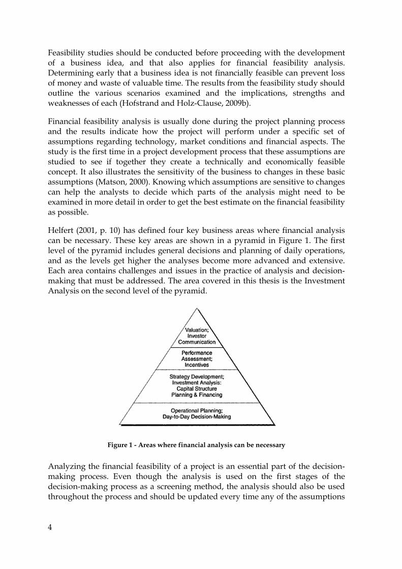
Helfert (2001, p. 10) has defined four key business areas where financial analysis can be necessary. These key areas are shown in a pyramid in Figure 1. The first level of the pyramid includes general decisions and planning of daily operations, and as the levels get higher the analyses become more advanced and extensive. Each area contains challenges and issues in the practice of analysis and decision-making that must be addressed. The area covered in this thesis is the Investment Analysis on the second level of the pyramid.
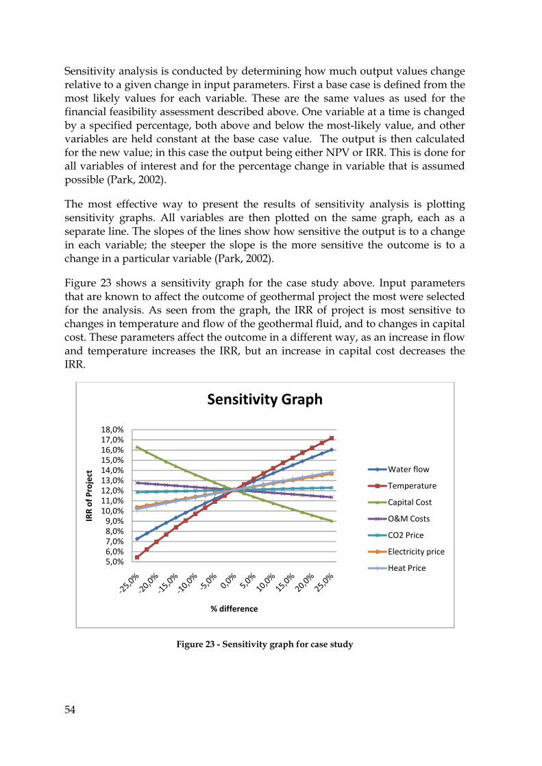
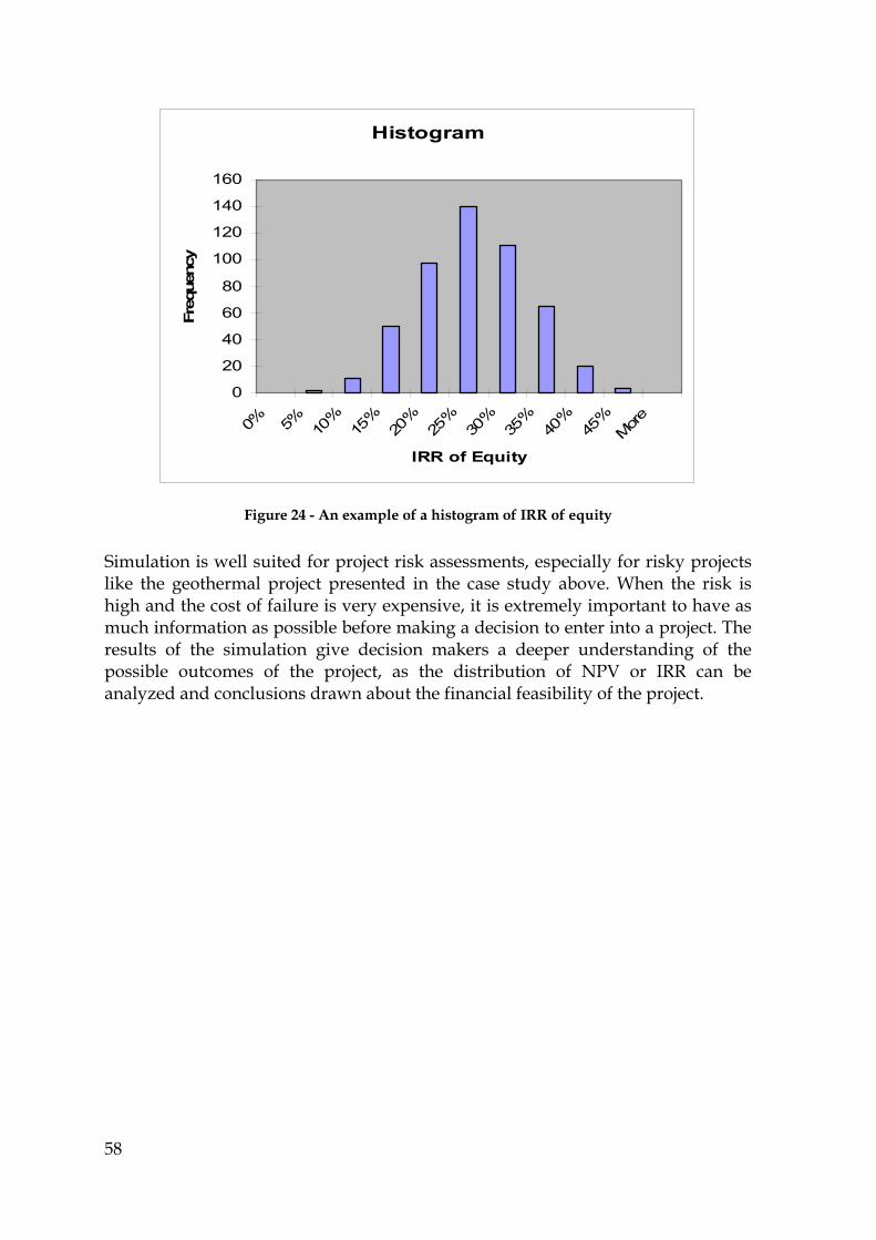
Figure 1 - Areas where financial analysis can be necessary
Analyzing the financial feasibility of a project is an essential part of the decision-making process. Even though the analysis is used on the first stages of the decision-making process as a screening method, the analysis should also be used throughout the process and should be updated every time any of the assumptions
5
it is based on changes. As Bennet (2003) puts it, if the results of the analysis show that the proposed project does not meet the return on investment requirements of the investor, the business idea is discarded. It is therefore very important to regularly update the analysis and verify that, given the newest information, the project is financially feasible.
2.1.2 Feasibility Study vs. Business Plan
Feasibility studies and business plans are two separate tools used for decision-making in project development. Both tools have common components, but should nevertheless not be confused as their roles are different. A feasibility study is a tool for investigating the viability of the prospective project. A business plan is a tool for planning the actions needed to take the project proposal from an idea to reality (Hofstrand and Holz-Clause, 2009b). As Matson (2000) sees it, the feasibility study refines the initial business idea, while the business plan uses information from the feasibility study to further prepare the project to evolve into an operating business.
A feasibility study is conducted on the very first stages of project development, before financing is secured and a go/no-go decision has been made. The purpose of the study is to reveal whether or not the project is viable from all aspects, such as financial, technological, market, etc. If the results of the study are positive, indicating that the project will be successful, much of the information from the study is incorporated into a business plan. However, if the results are negative, there is no need to create a business plan (Matson, 2000). A feasibility study usually analyzes several project alternatives or methods of achieving success. The purpose is to narrow the scope of the project and to identify the best scenario. A business plan only deals with one scenario, i.e. the scenario found to be most prominent by the feasibility study (Hofstrand and Holz-Clause, 2009b).
A business plan captures the goals and objectives of a business idea. It describes the purpose, strategy and tactics for the business activities, and assists managers in focusing their effort and identifying expected opportunities and obstacles. (Wild et al, 2007). The plan serves as a blueprint for the implementation of the project, as well as the actions taken during and after project implementation (Matson, 2000).
Feasibility studies and business plans are both very important in the decision-making process. A feasibility study is used throughout the whole process, first as a screening tool and then as a part of a business plan. As the financial feasibility of a project is a key element in a feasibility study, it is also a key element in a business plan. The business plan is often used as a sales document, helping the project owners to secure financing for the project. It is also used to persuade specialists to participate in the project and public authorities to give permissions for operations. The plan therefore needs to illustrate that the project is financially feasible, which is done by implementing the results from the financial feasibility analysis.
6
2.1.3 Conducting Financial Feasibility Analysis
Financial feasibility analysis is conducted by developing a base case financial plan and assessing the sensitivity of the profitability of the project, and the projected return, on the investor’s equity to various contingencies. Computer modeling is usually needed for analyzing these factors and can also be used in sensitivity analysis to analyze fluctuations in product price, changes in operating and maintenance cost, the effects of cost overruns, delay in completion, interruptions of project operations and other significant factors. (Finnerty, 1996)
When conducting a financial feasibility analysis, the analyst must start by making certain assumptions about the investment project. As the project gets closer to reality, the assumptions become more accurate and reliable, and thus also the analysis. If a reasonable change in an assumption could make the project change from successful to unsuccessful, the assumption should be considered a key element. Hard facts should be clearly distinguished from assumptions, and the sources for the facts and the rationale for key assumption noted (Matson, 2000).
Helfert (2001) states that the effort spent on taking the critical first steps at the beginning of the analysis will pay off in more focused and meaningful work and results. He proposes that the following should be considered before a financial feasibility analysis is conducted:
1. Nature and scope of the issue being analyzed;
2. Variables, relationships and trends likely to be beneficial to the analysis;
3. Use “ballpark” estimate of results to determine critical data and steps;
4. Precision is necessary for the analysis;
5. Reliability and uncertainty of available data;
6. Format of input data (cash flow or accounting);
7. Limitations of tools applied, and how these will affect the results;
8. Importance of qualitative judgments in the context of the issue, and how they rank in significance.
By reviewing and considering these points, the analyst will gain a deeper understanding of the task at hand, and more effort can be directed at areas where the most payoffs can be achieved from additional analysis (Helfert, 2001).
Hofstrand and Holz-Claus (2009a) suggest using the following outline when conducting financial feasibility analysis:
• Estimate the total capital requirements – seed capital, capital for facilities and equipment, working capital, start-up capital, contingency capital, etc;
7
• Estimate equity and credit needs - identify equity sources and capital availability, identify credit sources, assess expected financing requirements, and establish debt to equity levels;
• Budget expected costs and returns of various alternatives – estimate expected cost and revenue, the profit margin and expected net profit, the sales or usage needed to break-even, the returns under various production, price and sales levels, assess the reliability of the underlying assumptions of the financial analysis, create a benchmark against industry averages and/or competitors, identify limitations or constraints of the analysis, construct expected financial statements, etc.
As seen from this outline, financial feasibility analysis requires detailed information regarding the project operations and financial requirements. In addition to this, Finnerty (1996) considers the marketability of the project’s output (price and volume) the primary influencing factor on whether the project will be financially viable or not, given the assumption that the project will be completed on schedule and within budget. He therefore thinks that it is very important to conduct a market study and use the results as an input for the financial feasibility analysis.
The results of a financial feasibility analysis are only as reliable as the data used as input for the analysis. Data has to be collected from the project’s owners and from outside sources, and often specialists within the field of the project are needed to make estimates and forecasts, in order to get as accurate assessment as possible. The degree of precision in the input depends on the specific situation and it is often preferable to develop ranges of potential outcomes rather than precise answers. (Helfert, 2001)
2.1.4 Criteria for Financial Feasibility
In order to evaluate the financial feasibility of an investment project, relevant measurements or criteria need to be specified. Remer and Nieto (1995) categorize the evaluation methods into five basic types:
1. Net present value methods;
2. Rate of return methods;
3. Ratio methods;
4. Payback methods;
5. Accounting methods.
As seen, financial feasibility can be measured on the basis of accounting profits (from financial statements) or the projected cash flows of the project. Financial statements are records of actual financial activities of a business and are therefore not available for prospective projects, but projections of statements can be used to gain a better understanding of a project’s finances. The cash flows of the project
8
can also be projected and used to analyze the performance of the prospective project. The cash flow method is preferred over the accounting profits method, as the cash flow method considers the time value of money but accounting profits does not. Also, cash flows are always calculated in the same way but accounting profits can be calculated in several different ways, e.g. using different depreciation methods or inventory listings, which give different profit results. Hence, the cash flow method is considered more appropriate for evaluating the financial feasibility of investment projects.
There are several different cash flow based methods that can be used to measure the financial feasibility of investment projects, such as the Net Present Value (NPV), Internal Rate of Return (IRR), Annual Equivalent Worth (AE) and Benefit-Cost Ratio (B/C). These measures will be studied further below, as well as the Modified Internal Rate of Return (MIRR), which is a relatively new and still infrequently used criterion. Investors use these quantitative measures to help them decide whether to undertake an investment or not, based on their return requirements.
The payback period is another method that is sometimes used in financial feasibility analysis. The method determines when the project will break even, i.e. how long it takes for revenues to pay investment outlays. However, the method does not measure profitability, as it only measures the time it takes to recover the initial investment outlay but not the profit that is made after paying back the initial investment. The method ignores all revenues and cost after the payback period and does therefore not allow for the possible advantages of a project with a longer economic life. Also, the method does not recognize the time value of money, though that can be remedied by using the discounted payback method. Due to these drawbacks, the payback method is not suitable for measuring financial feasibility, and will therefore not be considered further in this thesis (Park, 2002).
Finally, financial ratios can be of use when analyzing financial feasibility. Financial ratios are calculated from the financial statements of a company and are generally only used for companies in operation. However, the projected financial statements can be used to calculate the relevant ratios in order to gain a better understanding of the performance of the project. Nevertheless, projected financial ratios should not be used independently as an analytical tool, but only in addition to the cash flow analysis.
Net Present Value
Net Present Value (NPV) is the difference between the present value of all cash inflows and cash outflows associated with an investment project. The NPV establishes whether or not the investment project is an acceptable investment, given the return the investor requires from the investment. Remer and Nieto (1995) claim that maximizing or minimizing the NPV of a project, depending upon
9
the situation, will provide the most efficiency, and as a result, the most profitability.
In order to calculate the NPV, the interest rate used for discounting the cash flows needs to be determined. The interest rate is often referred to as Minimum Attractive Rate of Return (MARR) and it represents the rate at which the investor can alternatively invest his money, i.e. the return of the most preferable alternative investment. The planning horizon of the project also needs to be determined, and the cash flows for each period of the planning horizon projected (Park, 2002).
The formula for NPV is:
1 1 … 1
1
where
An = Net cash flow at the end of period n;
i = MARR;
N = Service life of the project. (Park, 2002, p. 289)
If the NPV(i) is positive for a single project, the project should be accepted, since a positive NPV means that the project has greater equivalent value of inflows than outflows and therefore makes a profit (Park, 2002).
According to Park (2002) the decision rule for NPV is:
If 0, accept the investment;
If 0, remain indifferent to the investment;
If 0, reject the investment.
When comparing mutually exclusive alternatives the one with the greatest positive NPV is selected. According to Remer and Nieto (1995), when comparing alternatives it is important to use the same interest rate for all alternatives. All projects must also be compared over equal time periods, and sometimes adjustments have to be made for to account for this. In the case of mutually exclusive alternatives generating the same revenues, Park (2002) suggests comparing the projects on a cost-only basis. Then the project resulting in the smallest, or least negative, NPV should be accepted, since the objective is to minimize cost (not maximize profits).
10
Even though the NPV is a widely used criterion for financial feasibility it suffers from two limitations. First, the NPV assumes that periodic cash flows will be reinvested at the discount rate, which in reality is not always possible. Second, when considering two mutually exclusive projects of unequal size, the criterion’s ranking of the projects may give different results than from the Internal Rate of Return criterion, as will be discussed further below (Kierulff, 2008).
Annual Equivalent Worth
The Annual Equivalent Worth (AE) method is a variation of the NPV method. Instead of discounting all cash flows to present value, the AE method converts all cash flows to a series of equal cash flows over a specified time (Remer and Nieto, 1995). Usually the AE determines equal payments on an annual basis, and by that provides a basis for measuring investment worth. The AE is given by:
1
1 1
where
i = MARR;
N = Service life of the project. (Park, 2002, p. 346)
The decision rule for a single revenue project is:
If 0, accept the investment;
If 0, remain indifferent to the investment;
If 0, reject the investment.
The AE criterion is consistent with the NPV criterion in evaluating projects, i.e. if a project is accepted by the AE criterion it will also be accepted by the NPV criterion (Park, 2002)
The AE method has several advantages. When comparing mutually exclusive projects, the AE method does not require the projects to have the same service life, i.e. the projects do not have to be compared over equal time period as with the NPV method. The method also delivers simple and easily understood results, as it can be easier for some people to understand the prospects of a project by examining yearly costs/benefits per dollar, instead of examining one cash flow resolved to the present date (Remer and Nieto, 1995). In some situations the AE analysis is even preferred over the NPV analysis, such as when unit cost/profit is needed, when project lives are unequal or when consistency is needed in report formats (Park, 2002).
11
When comparing mutually exclusive projects the same applies for the AE analysis as for the NPV analysis, i.e. the project with the greatest positive AE is selected (Sullivan et al., 2006).
Benefit-Cost Ratio
The benefit-cost method is often used for public projects. The method compares project benefits to the cost of the project, and for the project to be viable, the benefits have to be greater than the cost. By definition, project benefits are the favorable consequences of the project to the public, and project cost is the monetary disbursement required of the government (Sullivan et al., 2006).
Park (2002) describes benefit-cost analysis as “a decision-making tool used to systematically develop useful information about the desirable and undesirable effects of public projects”. He defines three types of benefit-cost analysis problems:
1. Maximizing the benefits for any given set of cost;
2. Maximizing the net benefits when both benefits and costs vary;
3. Minimizing cost to achieve any given level of benefits.
The worthiness of a public project can be expressed by comparing the benefits (B) of the project to the cost (C) of the project by taking the ratio B/C, i.e. the Benefit-Cost ratio. The ratio is calculated as:
∑ 1∑ 1
where
Benefits at the end of period , 0;
Expense at the end of period , 0;
Project life;
Interest rate. (Park, 2002, p. 808)
The values of B and C have to be expressed in present value equivalents. For the project to be accepted the B/C ratio has to be greater than 1. The Benefit-Cost ratio yields the same investment decision as the NPV criterion. The decision rule is in fact the same, as seen from:
1
12
0
0
Park (2002, p. 809)
This shows that the Benefit-Cost Ratio could in fact be used to evaluate private projects and the NPV criterion could be used to evaluate public projects.
When comparing mutually exclusive alternatives, the Benefit-Cost Ratio cannot be used unless using incremental analysis. This is due to the fact that the ratio does not differentiate between investments of different sizes, e.g. a $10 investment and a $1000 investment. Then the incremental differences for each term are calculated and the B/C ratio taken from these differences (Park, 2002).
Internal Rate of Return
Internal Rate of Return (IRR) is a concept based on the return on invested capital in terms of a project investment, or as Park (2002) defines it: “IRR is the interest rate charged on the unrecovered project balance of the investment such that, when the project terminates, the unrecovered project balance will be zero”(p. 400). In other words, the investment has zero NPV at this rate of return, noted as . Therefore, serves as a benchmark interest rate, making investors able to accept or reject decision consistent with the NPV analysis. For simple investments, i.e. investments with only one sign change in cash flows, the IRR is the same as the (Park, 2002).
The IRR is equal to the rate of return for which the following function is zero:
1 0
(Park, 2002, p. 410)
Investors usually want to do better than breaking even in their investments. Their investment policy usually defines a MARR, in which case the IRR and the MARR can be used to decide whether a project is feasible or not. The decision rule for a simple project is as follows:
If , accept the project;
If , remain indifferent;
If , reject the project.
Howin th2002
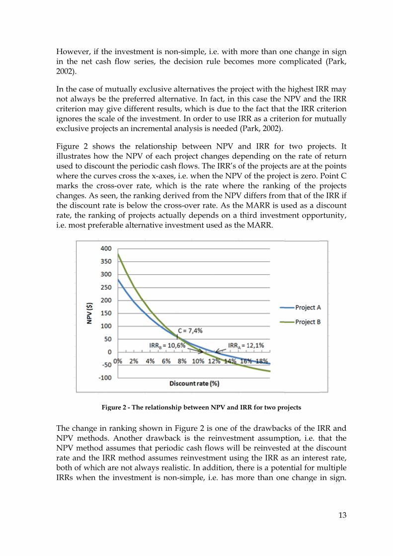
In thnot acriteignoexclu
Figuillususedwhemarkchanthe drate,i.e. m
The NPVNPVrate bothIRRs
wever, if thhe net cas2).
he case of malways be
erion may ores the scausive proje
ure 2 showtrates how
d to discouere the curvks the cro
nges. As sediscount ra, the rankimost prefer
Fi
change inV methodsV method a and the IR
h of which s when the
he investmh flow ser
mutually e the prefergive differale of the iects an incr
ws the rew the NPVunt the perives cross thoss-over raeen, the ranate is belowng of projrable altern
igure 2 - The
ranking ss. Anotherassumes thRR method are not alwe investme
ment is nonries, the d
exclusive arred alternrent resultsinvestmentremental a
lationshipV of each p
iodic cash he x-axes, ate, whichnking derivw the crosects actualnative inve
e relationshi
shown in Fr drawbackhat periodd assumesways realisent is non-
n-simple, i.decision ru
alternativesnative. In fas, which ist. In order
analysis is n
between project cha flows. Thei.e. when t is the ratved from t
ss-over ratelly dependestment us
p between N
Figure 2 is k is the re
dic cash flo reinvestmstic. In add-simple, i.e
e. with moule become
s the projecact, in thiss due to th to use IRRneeded (Pa
NPV andnges depee IRR’s of tthe NPV ote where tthe NPV de. As the Mds on a thised as the M
NPV and IRR
one of theeinvestmenows will bement usingdition, there. has mor
ore than ones more co
ct with thes case the Nhe fact thatR as a criteark, 2002).
d IRR forending on the projectf the projethe rankiniffers from
MARR is uird investmMARR.
R for two pro
e drawbacknt assumpe reinveste the IRR are is a potere than on
ne changeomplicated
e highest IRNPV and t the IRR cerion for m
two projthe rate of
ts are at theect is zero. ng of the p
m that of thused as a dment oppo
ojects
ks of the Iption, i.e. ted at the das an intereential for mne change
13
in sign d (Park,
RR may the IRR
criterion mutually
jects. It f return e points Point C projects
he IRR if discount ortunity,
IRR and that the
discount est rate, multiple in sign.
14
When that is the case it can be difficult to decide which IRR should be considered the right one (Kierulff, 2008).
According to Lee et al. (2009), the NPV is usually considered a superior method to the IRR. However, they also stress that the viability of the IRR should not be dismissed, since in some cases it may be better suited than the NPV.
Modified Internal Rate of Return
Over the past years there has been some criticism on the lack of robustness in the NPV and IRR methods, as these two measures can rank projects differently and assume reinvestment is always possible at the discount rate or IRR. The Modified Internal Rate of Return (MIRR), also referred to as External Rate of Return, is a measure that avoids these problems and provides a different and more accurate measure of financial feasibility (Kierulff, 2008).
The MIRR method is almost identical to the IRR method, except that the MIRR does not assume that all cash flows are reinvested at the calculated IRR, but instead assumes that all cash flows are reinvested at another rate, i.e. an external rate of return (Remer and Nieto, 1995).
The MIRR has not gained the same attention as NPV and IRR, and it is not commonly used for financial feasibility analysis within the industry. This might partly be explained by lack of academic support, but also some find it difficult to understand and compute. The MIRR may be challenging in practice because the user is required to specify both a return on investment that takes account of the risk of the investment, and a reinvestment rate given the risk associated with the future investments of the cash flows (Kierulff, 2008).
Fabozzi and Peterson (2003, p. 433) have listed the following steps involved in MIRR calculations:
1. Calculate the present value of all cash outflows, using a reinvestment rate as the discount rate;
2. Calculate the future value of all cash inflows reinvested at some rate;
3. Solve for rate – the MIRR – that causes future value of cash inflows to equal present value of outflows.
They also define the decision rule for MIRR as:
If , accept the project;
If , remain indifferent;
If , reject the project.
15
As with the IRR and the Benefit-Cost ratio, the MIRR cannot be used as a criterion for mutually exclusive projects unless using incremental analysis (Kierulff, 2008)
Even though the MIRR has not been commonly used in the past, Kierulff (2008) thinks that it is likely that the criterion will gain acceptance over time, as investors learn how to interpret the measurement and start using it in their decision making process.
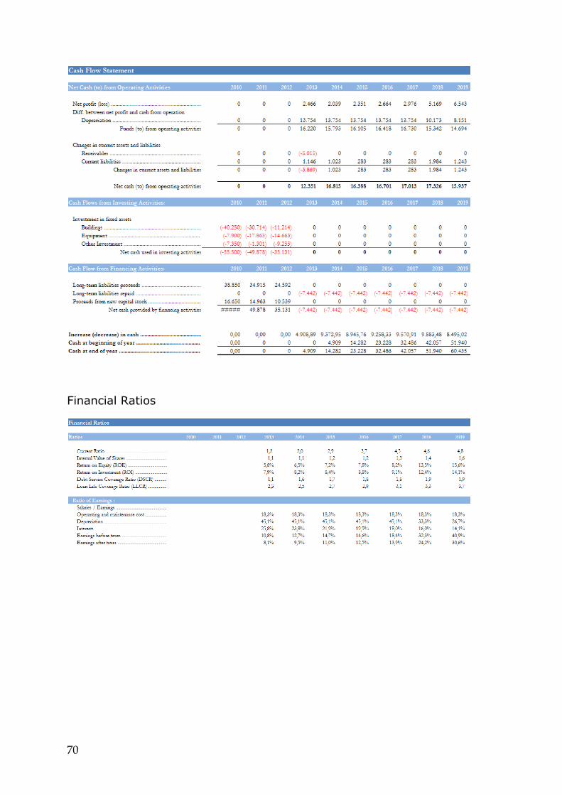
Financial Ratios
Financial statements are records of actual financial activities of a business entity and are therefore not available for prospective projects. However, by forecasting the revenues and costs of the entity, financial statements can be projected and analyzed to gain a better understanding of the performance of the entity. A decision on whether or not to invest in a new, unproven investment project should nevertheless not be based solely on the outcome of this analysis.
One way to analyze financial statements is to use the numbers from the statements to calculate financial ratios. By analyzing a series of financial ratios a clear picture is achieved of the entity’s financial condition and performance. Financial ratios can be used to compare two business entities within the same industry and also to compare an entity’s present ratios with that same entity’s past and expected ratios, which will indicate whether the entity’s financial condition has improved or deteriorated (Lee et al., 2009).
Financial ratios can be divided into five categories; liquidity ratios, asset management ratios, profitability ratios, market trend ratios and debt management ratios (Park, 2002). Only ratios that are appropriate and of use for prospective investment projects will be studied in this thesis. Ratios from four categories will be studied; liquidity ratios, profitability ratios, market trend ratios, and debt management ratios
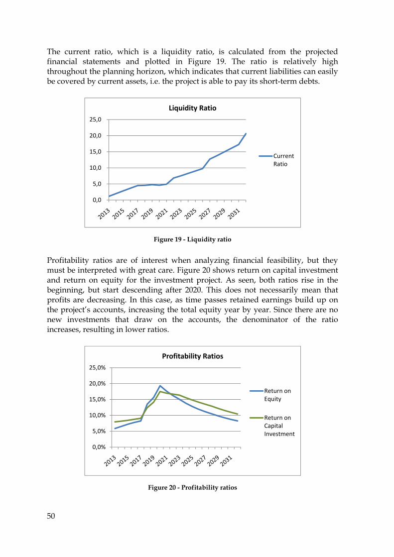
Liquidity Ratios Liquidity ratios are used to determine whether a business entity is able to pay off its short-term debts. The ratios show the relationship between the entity’s cash and other assets to its current liabilities (Park, 2002).
The current ratio is a liquidity ratio and it shows the relationship between liquid assets and payment commitments. It shows to which extent current liabilities are covered by current assets. The ratio is well established in practice, but has however some disadvantages, such as being time-related (i.e. a static figure) and too closely linked to the balance sheet. There is also a trade-off between liquidity and profitability, which should be taken into account when using the ratio for analysis (Wiehle et al., 2006).
16
The formula for the current ratio is:
(Park, 2002, p. 47)
If a business entity gets into financial difficulty and current liabilities rise faster than current assets, the current ratio will fall (Park, 2002). As a rule of thumb, an acceptable current ratio should total 200%. If the ratio is below 100% it is regarded as threatening to the entity’s existence (Wiehle et al., 2006).
Another liquidity ratio that is suitable for analyzing investment projects is the quick ratio, also known as acid-test ratio. The ratio is often used to determine how quickly a company is able to pay off its current liabilities.
The formula for the quick ratio is:
(Park, 2002, p. 47)
The quick ratio differs from the current ratio in that it excludes inventory, as while inventory may be fully paid for and have value, it may not necessarily be quickly converted into cash. As for the current ratio, the quick ratio should exceed 100% for the current liabilities to be covered by the entity’s cash position and total receivables (Wiehle et al., 2006).
Profitability ratios Profitability ratios show the combined effects of liquidity, asset management, and debt on operating results (Park, 2002). The ratios are used to measure whether a business entity is able to generate profits based on its earnings, expenses, and debt obligations. The ratios are compared to the same ratios from the previous year, or to ratios of firms within the same industry.
The return on investment (ROI) ratio is a profitability ratio that, when taken over time, helps in measuring the performance of the capital employed. It is a key indicator for investment decisions and it is comparable across different industries (Wiehle et al., 2006).
The formula for the return on investment ratio is:
17
The return on equity (ROE) ratio is a profitability ratio that measures the rate of return to stockholders. The higher the ratio, the more efficient is the use of stockholders equity, and the more return for investors (Groppelli and Nikbakht, 2006).
The formula for the return on equity ratio is:
(Groppelli and Nikbakht, 2006, p. 468)
The ROE ratio is highly relevant in practice and a good indicator for investments. However, it does not take debts into account and returns should be observed over the long term when using the ratio for analysis (Wiehle et al., 2006).
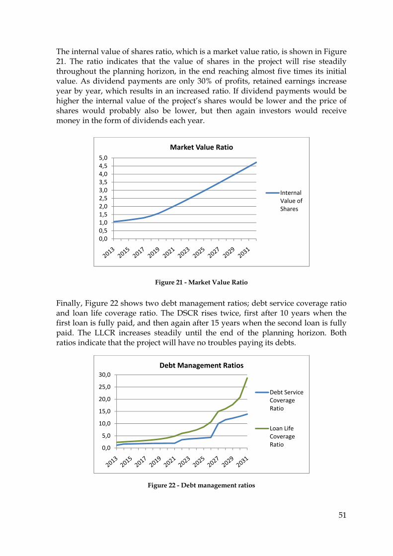
Market Trend Ratios Market trend ratios relate the business entity’s stock price to earnings and book value per share. The ratios give an indication of what investors think of the entity’s past performance and future prospects (Park, 2002).
The internal value of shares describes the relationship between equity and capital. The ratio is an indication of what the value of shares might be in the future. The higher the ratio is, the more value of shares.
The formula for the internal value of shares ratio is:
The ratio is dependent on dividend payments, since higher retained earnings increase the total equity, which results in a higher ratio.
Debt Ratios Debt ratios are used to show how a business entity uses debt financing, as well as the entity’s ability to meet debt obligations. Debt ratios are mostly used by creditors, e.g. when deciding interest rate levels for certain entities or industries (Park, 2002).
The Debt Service Coverage Ratio (DSCR) is used by lenders to assure that the prospective borrower will have sufficient funds to pay his debts. The ratio compares the cash flow available for debt service (interest and principal repayments) to the debt service for the same period.
18
The formula for the Debt Service Coverage Ratio is
(Navigator Project Finance, 2009)
The higher the DSCR is, the easier it is for the business entity to pay its debts.
The Loan Life Coverage Ratio (LLCR) is one of the most commonly used debt ratios in project financing. The ratio is similar to the DSCR, but the difference is that the LLCR considers the whole lifetime of the loan. The ratio shows the number of times the cash flow throughout the planning horizon can repay the outstanding debts.
The formula for the Loan Life Coverage Ratio is:
(Navigator Project Finance, 2009)
The period used in the NPV calculations is from the calculation year to the maturity of the loan. The discount rate used for the NPV calculations is usually the cost of debt (Navigator Project Finance, 2009).
2.1.5 Project Financing
Financing is one of the most essential parts of all projects. The financing structure can be very different between projects and it often depends on the type of the investment, the risk level of the investment, and the credit rating of the project owner. According to Fabozzi and Peterson (2003), the decision on how to finance a project is a very important managerial decision, since the different methods of financing obligate the project in different ways.
Project finance is a method of financing an economically capable project on the basis of the expected cash flows generated by the project. It is usually restricted to capital intensive projects and often involves a high proportion of debt finance. The cash flows of the project are segregated from the sponsoring organization, as the project is a separate entity. Project financing provides certain advantages over conventional financing, such as sharing of risk, reduced agency cost of debt and free cash flow, and expansion of sponsor’s debt capacity (Vishwanath, 2007).
Finnerty (1996) stresses that project financing should be distinguished from conventional financing, i.e. financing on a firm’s general credit. He states that “the critical distinguishing feature of a project financing is that the project is a distinct legal entity: project assets, project-related contracts, and project cash flows are segregated to a substantial degree from the sponsoring entity. The financing
19
structure is designed to allocate financial returns and risks more efficiently than a conventional financing structure”(p. 2-3).
According to Nevitt and Fabozzi (2000), projects are rarely financed independently on their own merits without credit support from sponsors that will benefit in some way from the project. They identify a wide range of available debt and equity sources for project financing, such as:
• International agencies (The World Bank, International Finance Corporation, area development banks, etc);
• Governments;
• Commercial banks;
• Institutional lenders;
• Money market funds;
• Commercial finance companies;
• Individual investors;
• Sponsors loans and advances.
Which sources are available and most suitable varies between projects, and a combination of sources is usually needed.
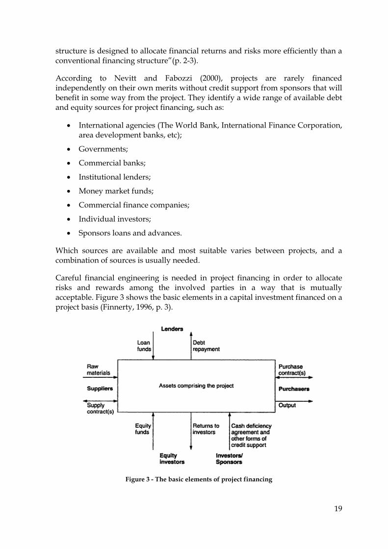
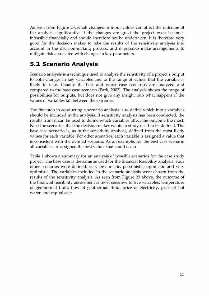
Careful financial engineering is needed in project financing in order to allocate risks and rewards among the involved parties in a way that is mutually acceptable. Figure 3 shows the basic elements in a capital investment financed on a project basis (Finnerty, 1996, p. 3).
Figure 3 - The basic elements of project financing
20
Several different types of project financing are commonly used in the construction industry. Some of them involve public-private partnerships, while others are fully private. Finnerty (1996, p. 195) has made the following list of questions to help find the most appropriate partnership structure:
• Who will be responsible for the design and construction of the project?
• Who will provide the construction funds?
• Who will arrange the financing?
• Who will hold legal title to the project’s assets and for how long?
• Who will operate the project facility, and for how long?
• Who will be responsible for each source of project revenue?
For a fully private project, the answer to all the questions is the private developer. However, some projects may have a mixture of private and public responsibilities (Finnerty, 1996).
Following is a list of some well-known project financing structures that utilize private investment to undertake public sector projects:
• BOO (build, own and operate): a private sector investor finances, builds and operates a project facility and receives title and ownership of it on an open-ended basis;
• BOT (build, operate and transfer): a project facility is built, financed and operated by a private sector entity. At the end of the concession period the facility is transferred back to the government;
• BOOT (build, own, operate and transfer): a project facility is built, financed, owned and operated by a private sector investor. At the end of the concession period the facility is transferred back to the government;
• BOOS (build, own, operate and sell): a project facility is built, financed, owned and operated by a private sector entity. At the end of the concession period the facility is transferred back to the government in a return for a residual value payment.
(Buljevich and Park, 1999, p. 216)
Nevitt and Fabozzi (2000) argue that the ultimate goal in project financing is arranging a borrowing which will benefit the sponsor and at the same time not affect his credits standing or balance sheet. They state that “the key to a successful project financing is structuring the financing of a project with as little recourse as possible to the sponsor while at the same time providing sufficient credit support though guarantees or undertakings of a sponsor or third party, so that lenders will be satisfied with the credit risk” (p. 2).
21
3 Financial Feasibility Assessment Model
The most effective way to analyze the financial feasibility of a prospective project is to use a specially designed financial feasibility assessment model. Many different scenarios have to be studied in the process of analyzing the financial feasibility of a project, and assumptions and project conditions often change during the decision-making process. Using a model for the calculations saves both time and money, and reduces the probability of calculation errors.
A financial feasibility assessment model can be designed and built in many different ways. The clearest and most effective way is to use a modular architecture, i.e. to build the model from several modular components. Each module represents a specific model function and modules interact by receiving and delivering data from one another. Modules make the model development and maintenance more focused and transparent, and also make it easier for the user to understand and visualize the functionality of the model.
Most financial feasibility models are custom made, as there are no standard model solutions on the market. The main reason is that investment projects are very diverse in nature, and appropriate model attributes vary from one project to another. It is therefore very complex to develop a model that can accurately estimate the financial feasibility of every project type.
The model presented in this thesis is designed for Microsoft Excel. Excel is a well suited tool for building financial feasibility assessment models. Different sheets can be used to organize different modules and different functions of the model. Most of all, Excel is a widely used application with a user friendly interface, so most people can learn how to use it without much effort. The model analyzes the financial feasibility of projects using cash flow methods, and also projects financial statements for further insight.
General model building principles and techniques will be presented below. The modular architecture used in the model will be introduced and the data flow through the model illustrated. Modular components will be presented and the functions of each module described.
3.1 Model Building
A financial model represents in mathematical terms the relationship among the variables of a financial problem. The model can be used to analyze different scenarios and make projections. The model should capture as many
22
interdependencies among variables as possible, and should be structured in a way that makes it easy to change the values of the independent variables and observe how the change affects the values of the key dependent variables (Sengupta, 2004).
When designing and building a model, several things should be kept in mind. Sengupta (2004, p. 132) lists the following key steps in the development of a financial model:
1. Understand the expected uses of the model and the required outputs;
2. Collect historical data for the company, its industry, and its major competitors;
3. Understand the company’s plans and develop a comprehensive set of modeling assumptions;
4. Build the model and debug it;
5. Improve the model based on feedback.
As seen from these steps, is imperative to understand the requirements and expectations of the model’s users. The objective of building the model is to fulfill these requirements, and therefore they have to be kept in mind throughout the whole design and implementation process. All model assumptions should be thoroughly studied and the model builder needs to make sure that they are appropriate for the object being modeled. Finally, it is very important that the model builder uses feedback from model owners and users to improve the model, to make it the best representation of reality as possible.
Tjia (2004, p. 14) suggests considering the following key design principles when building a model:
• Keep the model simple;
• Have a clear idea of what the model needs to do;
• Be clear about what the users want and expect;
• Maintain a logical arrangement of the parts;
• Make all calculations in the model visible;
• Be consistent in everything you do;
• Use one input for one data point;
• Think modular;
• Provide ways to prevent or back out of errors;
• Save in-progress versions under different names, and save them often;
• Test, test and test.
23
These principles show that it is very important to realize the purpose and functions of the model before building the model. The model building should also be organized before commencing. Thinking modular is an essential principle, as breaking the task at hand into smaller and simpler components makes improving and testing the model easier.
Having a clear model objective makes the model design and implementation more focused, which results in a better model. The model should be transparent and easily understood by the user. It should also be accurate and reliable, so the user can trust the results and confidently use it in the decision-making process. According to Mun (2006), it can be beneficial to keep several rules of thumb in mind during the model building process. Inputs, calculations, and results should be separated. Inputs should be color coded and input parameters named to avoid mix-ups. The model should be protected against tampering by password protecting workbooks and formulas, and changes to the model should be tracked. Finally, the model should be user-friendly, e.g. by using data validation and error alerts.
3.2 Model Architecture
The financial feasibility assessment model is built from several different modules, each representing different functions of the model. By using a modular architecture the functions of the model become more visual to the user and it becomes easier to maintain and improve the model, since each module can be considered a separate part of the model.
The modules have different functionalities. Each module takes in data, either as input from the user or as output from other modules. The modules process the data and deliver various outputs, depending on the function of the module. By building the model out of several modules, the model builder can concentrate on one module at a time and separate the function of that module from other modules. By doing this, the model building becomes more focused and effective, resulting in a robust and reliable model. Modules also make it easier for the user of the model to understand and use the model, as the user only needs to enter data into the input module and obtain results from the results module.
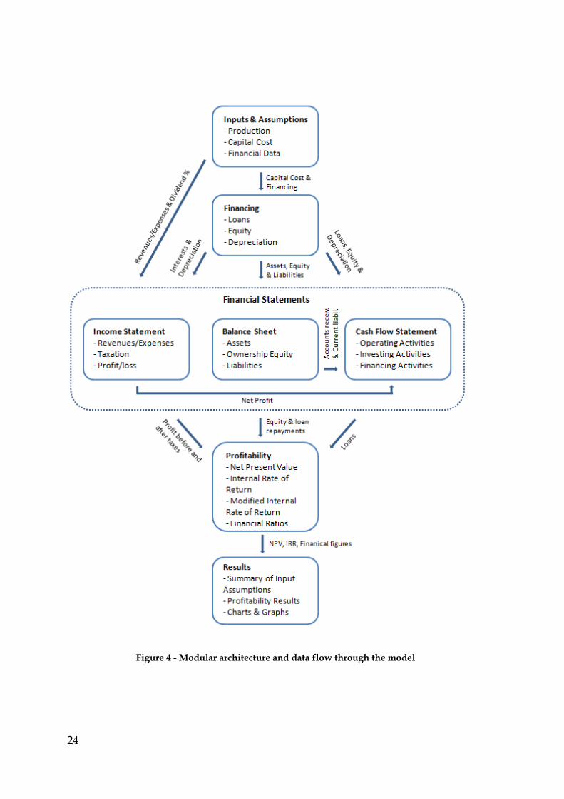
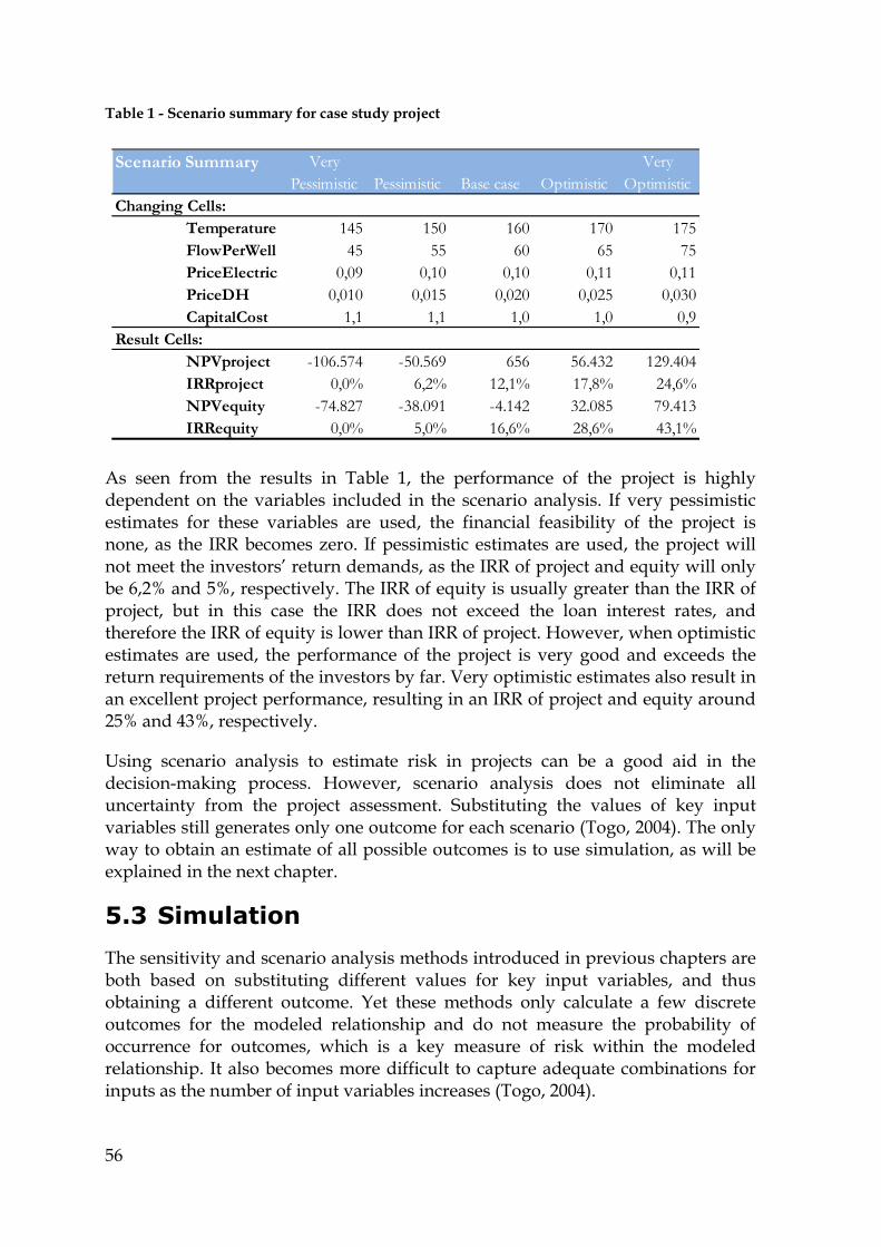
Figure 4 shows the modular architecture of the model. It illustrates how modules interact and how data flows between modules. The inputs and assumptions module is the only module that users can enter data into. Other modules process these inputs and assumptions and execute calculations needed for the assessment. Module functions will be discussed in more detail in next chapter, Modular Components.
24
Figure 4 - Modular architecture and data flow through the model
25
3.3 Modular Components
3.3.1 Inputs and Assumptions
The inputs and assumptions module collects all necessary information and assumptions regarding the project, which are needed for the financial feasibility assessment. All inputs are located in this module and input cells colored in a specific color to place emphasis on which cells the user has to fill in. All other cells are locked in order to prevent disarrangement of formulas and links between cells.
Input data usually includes information on generation of revenues and associated expenses, capital cost, operation and maintenance cost, financing requirements, taxes and depreciation rates, the MARR of project and equity, dividend payments and other financially related assumptions.
Inputs required for the analysis can vary between investments and industries. Therefore feasibility models often need to be adjusted for the type of investment under consideration.
3.3.2 Financing
The financing module calculates the financing requirements of the investment project. The calculations are based on capital cost figures and financing options available for the project.
A new method is used in the model to estimate the financing requirements of the project with optimization. The financing requirements are based on capital cost and working capital, which is the capital needed to pay short-term debts and continue operations. Capital cost figures are taken from the input and assessment module but the working capital is found using optimization. If the construction period overlaps the operations period, working capital can sometimes be covered with profits from operations, and then the working capital figures are negative. Since loans are expensive, the optimization uses as much money as possible from operations to cover the working capital. The optimization is done using the Solver application in Excel. The solver is set to maximize the net present value of equity by changing the working capital, and by constraining the cash account, the equity drawdown and the loan drawdown to be greater than or equal to zero. The optimization can be set forth as follows:
Objective function:
max
By changing:
26
Constraints:
0
0
0
Financing requirements for each year are determined from the results of the optimization. Financing of the project is covered with both paid equity and drawdown of loans. It is economically best to borrow only what is needed for the project, given the paid equity. Borrowing more than needed will result in higher interest expenses and the excessive money will not be of use in the project, but end up as surplus on the project’s accounts.
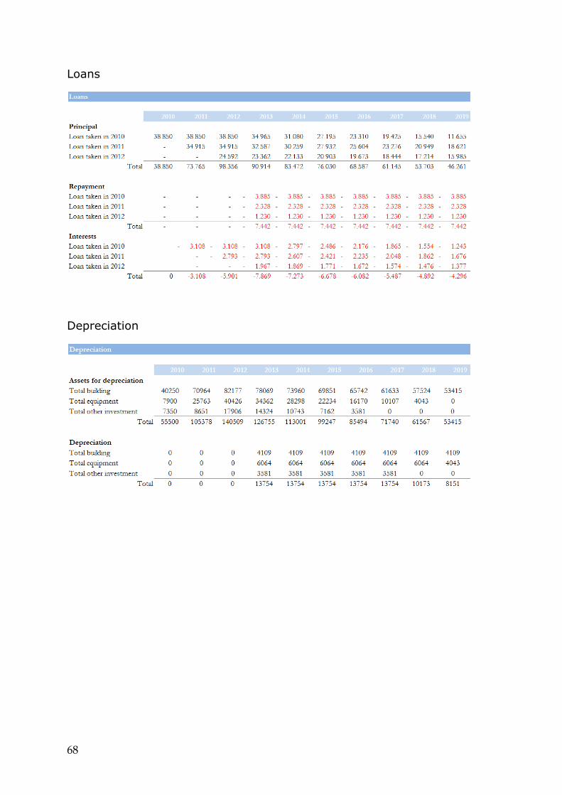
It is up to the project’s owner to decide what level of details should be included in the loan calculations, such as refinancing possibilities, interest rates and refinancing interest rates, whether grace periods are available, and whether both short and long term financing should be considered. It also needs to be decided whether to define these for each loan separately or assume that all loans have the same properties. Loan interests are calculated based on the principal of the loan at the end of the previous year. Loan management fees should be included in the calculations, according to the terms given by the lender.
Several methods can be used to depreciate assets, such as the straight-line method, the declining-balance method and units-of-production method (Sullivan et al., 2006). The straight-line method is widely used, e.g. in Iceland, and will therefore be used in this thesis. In most countries, depreciation and amortization are the same, but in some countries amortization is used for intangible assets, e.g in the United States. Although depreciation expenses are not actual cash flows, depreciation has an important impact on cash flows by reducing taxable income and thus taxes (Park, 2002). In the model, different depreciation categories are defined and the investment is depreciated according to regulations in the respective country.
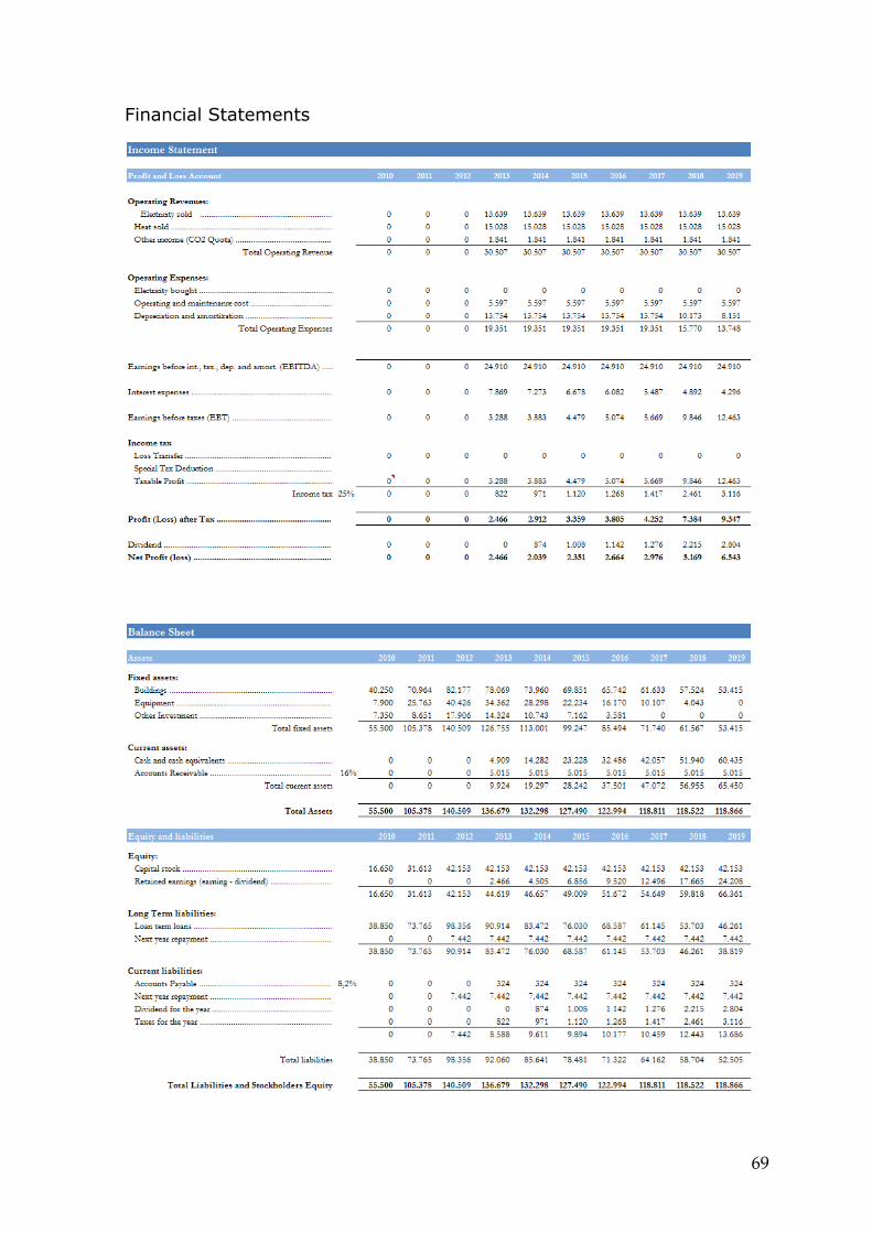
3.3.3 Income Statement
The income statement shows the performance of the investment project in each period, i.e. it reveals the profit or loss generated by the project. The performance is measured at regular intervals and in this model it is done annually. Investors can use figures from the income statement to determine whether their investment will give them an acceptable return.
The income statement lists the operating revenue and operating expenses of the project, which are then used to calculate the EBITDA (Earnings before Interests, Taxes, Depreciation and Amortization). EBT (Earnings before Taxes) can then be
27
calculated by extracting interest expenses, depreciation and amortization from the EBITDA.
Income tax is calculated on the income statement. Taxable profit is the EBT minus loss transfer (if it is allowed to transfer losses between years). The income tax paid to the government is a percentage of the taxable profit, and it depends on tax regulations in the respective country. Profit after tax is then calculated, as well as the net profit or loss, i.e. profit after dividend has been paid.
The income statement uses issued bills to show the performance of the project, not the actual cash flows, since not all invoices have been paid at the end of a period. The difference lies in accounts payables and account receivables.
3.3.4 Balance Sheet
The balance sheet summarizes the financial position of a project at a given point in time. It shows the project’s balances, i.e. its assets, ownership equity and liabilities. It is a statement of the project’s investments and the value of the claims to the payoffs from those investments (Penman, 2001).
Assets are divided into fixed assets, such as buildings and equipment, and current assets, which consist mainly of the cash account, inventory and accounts receivables. The balance sheet shows the assets of the project at the end of each fiscal year, and the changes in assets between years, which can be due to e.g. new investments (increase in assets) or depreciation (decrease in assets).
Ownership equity is divided into capital stock and retained earnings. Capital stock is the equity put forth by the owners of the project. Retained earnings are the accumulated net profits of the project, i.e. earnings after dividends have been paid.
Liabilities are divided into long term liabilities and current liabilities. Long term liabilities are the long term loans taken to finance the project, i.e. all loan repayments that are not due in the next year. Current liabilities are mainly next year’s loan repayments and taxes, as well as accounts payable and dividends.
By definition the assets of the project are equal to the total liabilities and owners equity of the project. This is checked in the balance sheet of the model to make sure that the financial statements are correctly constructed.
3.3.5 Cash Flow Statement
The cash flow statement shows the actual cash flows of the project, i.e. the flow of cash and cash equivalents to and from the project. It shows how cash is generated and used during each period. The statement shows the cash flow related to operating, investing and financing activities (Penman, 2001).
28
The cash flow statement can be used to analyze the following:
• The source of financing for business operations – internal or external sources of funds;
• The company’s ability to meet debt obligations;
• The company’s ability to finance expansion through operating cash flow;
• The company’s ability to pay dividends to shareholders;
• The company’s flexibility in financing its operations.
(Fabozzi and Peterson, 2003, p. 138)
The cash flow statement is divided into three segments. Cash flow from operating activities consists of the net profit (adjusted for depreciation, since it involves no cash outlay) and changes in current assets and liabilities. Cash flow from investing activities consists of the purchase or selling of fixed assets. The cash flow is negative when new assets are purchased and positive when assets are sold. Cash flow from financing activities consists of changes in debt or equity, i.e. new loans taken, repayments of loans and new equity.
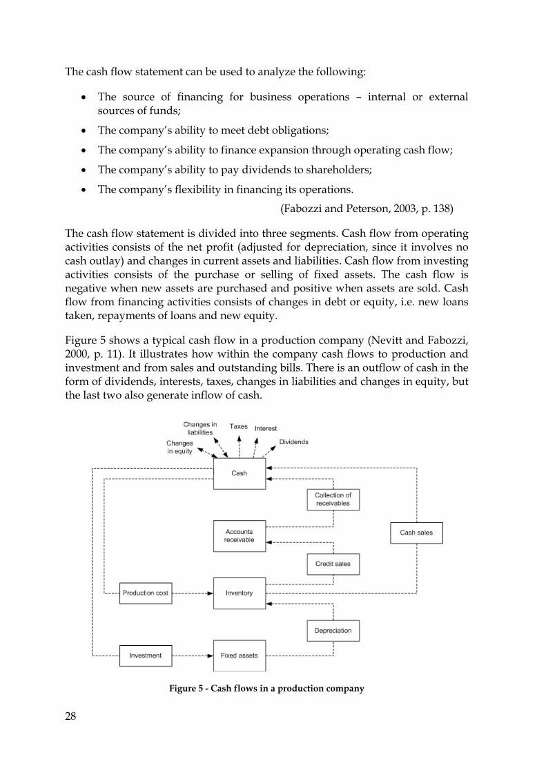
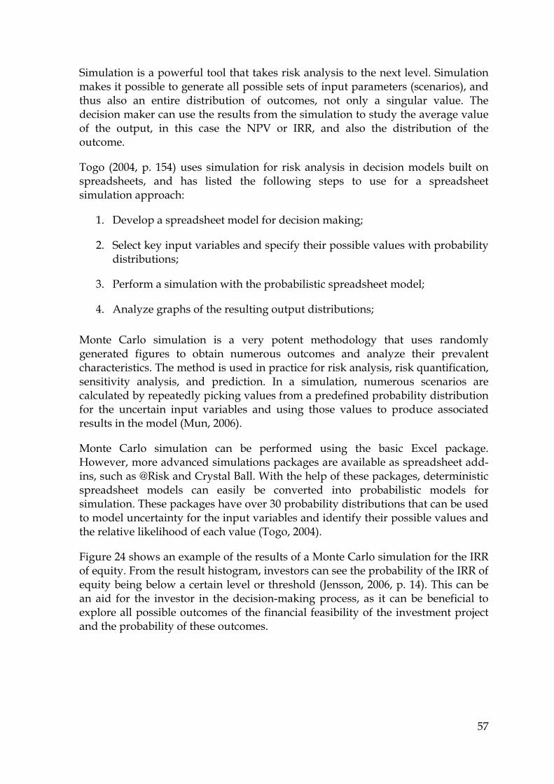
Figure 5 shows a typical cash flow in a production company (Nevitt and Fabozzi, 2000, p. 11). It illustrates how within the company cash flows to production and investment and from sales and outstanding bills. There is an outflow of cash in the form of dividends, interests, taxes, changes in liabilities and changes in equity, but the last two also generate inflow of cash.
Figure 5 - Cash flows in a production company
29
As stated above, there is a difference between the Income Statement and the Cash Flow Statement. The Income Statement shows the performance of the project with respect to issued invoices, without taking outstanding invoices into account. Profits are calculated taking depreciation into account, and taxes and dividends are listed on the year of calculation of these figures. The Cash Flow Statement however shows the performance of the project with respect to the actual cash flowing though the project. Funds from operating activities are listed, which is the profit of the year without taking depreciation into account. Finally, taxes and dividends are listed in the year of payment. This difference between the statements can give different indications on financial feasibility, as the net profit calculated on the income statement can indicate that the project is performing very well even though the cash funds of the project have decreased and the project has performed poorly. It is therefore not enough to analyze the financial feasibility of a project by just looking at one and discarding the other. However, the cash flow statement is more important for financial feasibility analysis of investment projects, as it considers the time value of money.
3.3.6 Profitability
The profitability of the project is calculated from the project’s cash flows. In this model the NPV, IRR, and MIRR are used as profitability criteria. The first two are the most commonly used criteria for profitability assessment and are therefore most suitable. The MIRR is, as discussed above, an improved version of the IRR, and should be presented for a better view of the project’s profitability. All of the criteria are calculated with Excel’s built-in functions. The criteria are calculated for both project and equity. Calculations of the criteria for the project are independent of the financing structure of the project, i.e. it is assumed that all funding comes from equity. The calculations involve the cash flows of the project and the capital investment. On the other hand, calculations of criteria for equity take funding of the project into account by including debt service in the calculations. The calculations involve the net cash flows of the project and equity payments from owners.
Financial ratios are also calculated within the profitability module, using figures from the financial statements.
3.3.7 Results
The results module is used to report and deliver the results of the financial feasibility assessment. The module is designed so that all results can be printed and delivered to the user. Input assumptions are stated and results presented in a clear way, giving the user the best overview of the results as possible.
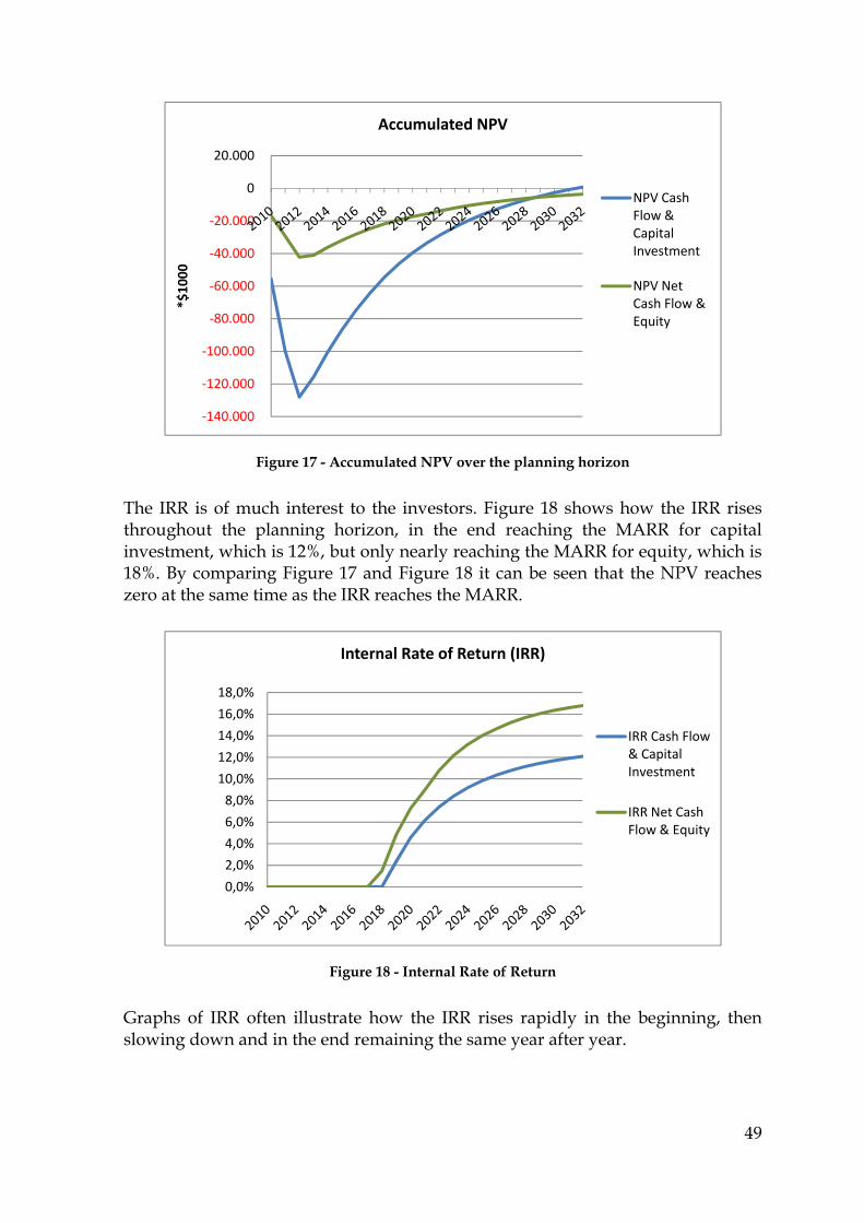
The most important results are the NPV and IRR, since the investors use these figures to determine whether the investment meets their profit demands. The IRR and the Accumulated NPV are shown graphically, as well as the project’s cash flow throughout the planning horizon of the project. Breakdown of income and
30
expenses is also shown graphically in order for the investors to realize which factors have the most impact on the operation.
Financial ratios are presented graphically in the results module. The ratios are calculated over the planning horizon of the project and give the decision maker a good indication of the project’s performance and a deeper understanding of the financials of the project.
31
4 Case Study – A Geothermal Power Plant
The purpose of this case study is to demonstrate how a potential investment project is evaluated using a financial feasibility assessment model. A geothermal power plant construction project will be used as a case example. The case selection is motivated by Iceland’s unique position of having over 70 years experience with harnessing and utilizing geothermal energy for producing electricity and useful heat. In 2006, geothermal plants generated 25% of the electricity in Iceland, and 90% of the heat (Orkustofnun, 2009).
The model used for the case study was designed and developed specifically to analyze the financial feasibility of geothermal projects. The objective of the case study is to estimate the feasibility of building a geothermal cogeneration plant, i.e. a plant producing electricity and useful heat simultaneously. The data used in the case study is fictive, but both technical data and capital cost data is based on real projects in order to keep the case study as realistic as possible.
4.1 Geothermal Energy Utilization
Geothermal energy is one of the world’s renewable energy sources and the technology of producing electricity from geothermal energy is a well-established industry, as well as using the energy for useful heating. Over the past years there has been a worldwide awakening concerning the negative effects of global warming. This has made geothermal energy a more attractive energy alternative, as it is a low-polluting energy source, compared to most other sources. Geothermal energy is also very reliable, with up to 95% availability rate, so it is well suited to supply base load electricity.
Geothermal energy can be utilized in various ways. Fresh geothermal water can be used for domestic, commercial and industrial needs. Heat can be used for heating and cooling, and steam or high temperature fluids can be used for electricity production. A variety of geothermal products and byproducts can also be used for agricultural and industrial applications. Furthermore, the geothermal resource is relatively constant and can therefore be used as a source of either base load or peaking power (International Energy Agency, 1991).
According to the International Energy Agency (1991), there are several requirements for electricity generation from geothermal energy, such as a moderate or high temperature resource, adequate reservoir volume and sufficient reservoir permeability. The energy conversion system used for the electricity
32
generation depends on the state of the geothermal fluid and its temperature. Available conversion systems are:
• Dry steam – used for vapor-dominated reservoirs. The steam is led directly through the turbine/generator unit for electricity production;
• Flash steam – used for liquid-dominated reservoirs with temperature in the range of 150°C-200°C. The geothermal fluid is flashed to steam, which is then directed through a turbine. In some cases it is possible to flash the fluid more than once;
• Binary cycle – used for liquid-dominated resources which are not hot enough for flash steam production. The geothermal fluid passes through heat exchangers where heat is transferred to a working fluid with a low-temperature boiling point. The working fluid is then used to drive the turbine/generator unit. Corrosion and scaling problems are avoided by using binary systems, as the geothermal fluid is in a closed system and can be kept pressurized and free of oxygen.
(International Energy Agency, 1991, p. 44)
Geothermal power plants have high capital cost but are still very cost effective. No fuel is required in the power production, and therefore the financial feasibility is unaffected by fluctuations in fuel cost. However, drilling wells to extract geothermal fluid is very expensive and exploring the geothermal resource involves considerable risk. The feasibility of the project therefore depends on whether or not the exploration is successful.
Since geothermal power plants have relatively low emissions of greenhouse gases (GHG), using geothermal energy instead of fossil fuels can help reduce global warming. If a power plant is located in a developing country, it can earn carbon credits through the Clean Development Mechanism (CDM) established under the Kyoto Protocol. According to the CDM, a low polluting power plant can sell the emission offset it achieves. A district heating unit however needs to replace another, more polluting, district heating system to be able to sell emission offsets. Geothermal power plants have lower emissions than most other types of power plants and are therefore ideal for replacing highly polluting power plants, such as fossil fuel power plants. Trading CO2 emissions improves the economics of a geothermal project, since selling CO2 quota generates a positive cash flow to the project and therefore increases its financial feasibility.
Developing a geothermal project is technically complicated and it can take many years to develop a geothermal green-field into an operating power plant. The process involves landowners, utilities, consumers (public and/or private), and authorities.
33
4.2 The Model
The model used for this case study is an Excel-based financial feasibility assessment model. The original model, which this version is based on, was designed and developed by an Icelandic company, specialized in development and construction of geothermal power plants. The model has been under development for a few years and is constantly being improved and updated. Before the model was created the company had to outsource the making of feasibility studies to other companies. Now the model is used to evaluate all potential investments and projects, which saves the company both time and money. Due to a confidentiality agreement, the owner of the original model cannot be identified.
The model uses projected cash flows to calculate the financial feasibility of prospective geothermal projects. The model has several functions; it calculates electricity and/or heat production capacity, given the characteristics of the geothermal resource, obtains projected financial statements, and calculates the profitability of the prospective project. The model uses thermodynamic formulas to calculate electricity and heat production. Income calculations are based on the estimated production, forecasted energy prices, and if carbon trading is allowed, income from selling CO2 quota. The model uses constant monetary units for both income and expenses, i.e. it does not take inflation into account. Using inflation does not give any additional information on the financial feasibility, as it is assumed that all revenue and cost components are equally affected by inflation.
The planning horizon used for the analysis can be chosen as appropriate for each project being analyzed. A typical horizon for the geothermal industry is 20 years of operation, in addition to the construction period, which can be up to 10 years. The construction period can also be divided into phases, which could be the case if for example the investors want to test the geothermal resource and power plant under operation before making a decision to build a new unit or expand the existing plant. Then the construction period overlaps with the operations period.
The model is ideal for analyzing the financial feasibility of projects at any stage of the decision-making process. It is robust, easy to use and gives a good indication on the financial feasibility of the project. The model can be used for initial screening and pre-feasibility assessments of geothermal projects, as well as for highly detailed assessments for business plans. Before entering into a project it is also necessary to do a full feasibility assessment of the project, taking into account all aspects of the project, not only the financial. Then, as information become available, the design parameters of the plant need to be calculated with more detail and precision and the financial feasibility assessment updated accordingly.
When building a model for financial feasibility analysis of geothermal projects, as with any modeling of real systems, it is very important to have a good knowledge of the technology used. For geothermal projects this includes knowledge of
34
geothermal reservoirs types, different energy conversion systems, power plant and heating unit design and operation, etc. The model builder does not personally have to know everything about the object being modeled, but has to have access to specialist within all related fields.
As the project progresses and the power plant has been designed, the production capacity of the power plant should be estimated from the design parameters of the plant. The financial feasibility estimate should then be updated, using the estimated production capacity to obtain a more accurate estimate on the financial feasibility.
Below is an overview of the inputs and assumptions used in the model, the calculations executed in the model, and the results from the financial feasibility analysis conducted with the model.
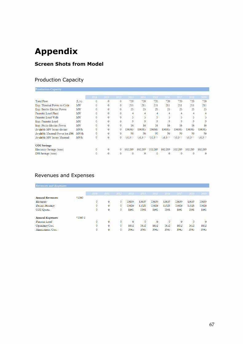
4.2.1 Model Inputs and Assumptions
All inputs and assumptions are located in the same sheet of the model. All input cells are colored in grey, which makes it easier for the user to realize whether or not all required inputs have been entered. This is done in order to avoid mistakes and to make the model more user-friendly. The model uses annual periods, and as stated above the model is based on fixed terms using real monetary figures and thus does not take inflation into account.
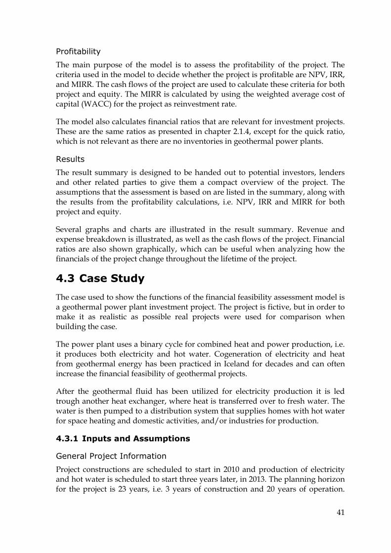
General Project Information
General information on the proposed project includes all information that is not technical, financial or related to marketing. Following are the general inputs of the model:
• Date – the date of publication of the analysis;
• Currency – the currency of the project;
• Beginning of project – the year that the project will begin;
• Beginning of operation – the year operation will start;
• Years of operation – the number of years of operation included in the calculations.
Production
Production information includes all decisions taken regarding the production of the power plant. This includes how the energy will be utilized and the utilization method. If the proposed project is located in a developing country and carbon trading is possible, the CO2 savings from the plant need to be estimated and revenues from CO2 quota sales included in the cash flow calculations. Following production inputs are required for the analysis:
35
• Produce electricity (yes/no) – decide whether or not the plant will produce electricity. This depends on the resource and a decision is usually taken after the resource has been explored.
• Provide district heating (yes/no) – decide whether or not the plant will produce hot water for district heating. The plant can produce either electricity or hot water, or produce both at the same time.
• Sell CO2 quota (yes/no) – if carbon credits can be achieved in the respective country, a decision needs to be taken on whether or not to include revenues from selling CO2 quota in the financial feasibility analysis. This has to be decided for both electricity and hot water production.
• CO2 Savings – if revenues from selling CO2 quota are included in the analysis, the CO2 savings of the plant will have to be estimated. In many countries, the CO2 saving of electricity production is calculated as the average of CO2 emissions from all power plants delivering to the grid, and in these countries this average should be used.
Wells and Fluid
In order to determine the production capacity of the power plant, several technical parameters need to be estimated. These parameters involve e.g. the flow of geothermal brine to the power plant and several temperatures at different stages of the plant work cycle. Technical parameters are usually estimated after the reservoir has been explored and an exploration well has been drilled and tested. Following are the inputs and assumptions of wells and fluid required for the analysis:
• Number of wells – the total number of production and re-injection wells, i.e. both new wells and previously existing wells.
• Well temperature – the temperature of brine flowing from wells needs to be estimated in order to estimate the production capacity of the plant. This is usually estimated from exploration well testing.
• Well flow – the flow of brine from wells is a key factor in the production capacity of the plant. The flow from wells influences how many wells need to be drilled for production.
• Brine’s specific heat – the specific heat, i.e. the energy content, of the geothermal brine influences the production capacity, as it determines how much energy can be extracted from the brine.
• Temperature of returned brine – the temperature of the brine after it has been through the electricity generation part of the plant. This temperature influences the plant’s production capacity of hot water.
• Temperature back to well – the geothermal brine is re-injected to the geothermal reservoir and a re-injection temperature has to be defined. The chemistry of the geothermal fluid often affects the re-injection temperature,
36
as the fluid can in some cases be corrosive and cause scaling problems, which then again affects the financial feasibility of the project by increasing the maintenance cost of the power plant. The difference between the temperature after the electricity generation part of the plant and the re-injection temperature determines the capacity of hot water production of the plant.
Power Plant
Inputs for the power plant are related to the operations of the power plant. Some inputs can be estimated based on a specialist’s knowledge of geothermal power plants, but other have to be based on exploration well testing and the production cycle used in the power plant. Following are required inputs related to the power plant:
• Plant running hours – the number of hours that the plant will operate each year. This factor is very high for geothermal power plants, or up to more than 95% of the year.
• Plant power efficiency – often estimated based on a specialist’s knowledge or industry average for similar plants. On later stages the efficiency is calculated with more precision.
• Operation cost – all cost related to operations, such as management cost, labor cost, etc. In this model the operation cost is assumed to be a percentage of the total cost of constructing the power plant, i.e. the part of total capital cost that is related to the power plant (not wells).
• Maintenance cost - all cost related to maintenance of the plant, such as spare parts, equipment repairs, etc. In this model the maintenance cost is assumed to be a percentage of the total capital cost.
• Parasitic load – the own electricity consumption of the power plant needs to either come from the electricity produced at the plant or purchased from the grid. Therefore a decision has to be made on whether to use own power or external power for parasitic load. In some cases it might be cheaper to buy electricity from the grid than to use the electricity produced by the plant, e.g. in Germany, where there is a higher price for renewable energy. In that case parasitic load should be bought from the electricity grid and all electricity produced should be sold.
• Plant parasitic need – the percentage of the plant’s production that is needed for own use, i.e. to run the plant itself.
• Production pump power – if a pump is used to pump the geothermal fluids from the production wells, the power needed to operate the pumps has to be estimated.
37
• Re-injection pump power - if a pump is used to pump the geothermal fluids down the re-injection wells, the power needed to operate the pumps has to be estimated.
Market
Market conditions are very different between market areas and thus have to be analyzed for each case. Market conditions can often change rapidly and therefore all assumptions regarding the market should be updated regularly. Following are the market information required for the analysis:
• Electricity sales price – the price of electricity sold from the plant. Estimate is based on either forecasted spot market price or a power purchase agreement.
• Electricity purchase price – used if the parasitic load is bought from the grid, i.e. if the sales price of electricity is higher than the price of electricity purchased from the grid.
• Hot water sales price – the price of hot water sold from the plant. Estimate is based on either forecasted price or a sales contract with e.g. local municipalities or industries.
• CO2 price – estimated market price of CO2 quota, based either on forecasted spot market prices or a sales contract.
• Market size – estimated market size for both electricity and hot water. In most cases there is no constraint on the selling of electricity, i.e. the plant can sell all the electricity it can produce. The market for hot water is however sometimes limited and therefore needs to be analyzed with a market study.
Capital Cost
Geothermal power plants have high capital cost compared to many other power plant types. However, geothermal plants have lower operation and maintenance cost than other types of power plants. Therefore the capital cost is a large part of the overall cost of the geothermal power plant.
The total capital cost of geothermal power plants is influenced by many factors. These factors include the technology used for electricity and heat production, the size of the plant, the depth of the resource, the chemistry of the geothermal fluid, etc. The total cost is divided into five categories in the model: preparatory phase and general project management, drilling, civil engineering, electrical and mechanical (el-mech) engineering, and testing and finishing. The calculation of these cost components is not done within the model, but imported from other documents as input.
38
The preparatory phase and general project management includes many cost components. It includes exploring and mapping the reservoir, drilling and testing an exploration well, doing environmental surveys, attaining land rights and production permits, etc.
Drilling cost is usually the largest component of the capital cost. Drilling production and re-injection wells is very expensive and there is always some risk of failure. It is often used as a rule of thumb that 5-10% of all wells will not qualify for production. Cost associated with drilling include the lease of the drill rig, all material used for drilling, casing of wells, etc.
The cost of constructing the power plant is divided between civil engineering and electrical and mechanical engineering. The cost includes the power plant building, the turbine-generator, pipelines, electrical equipment, etc.
The final category is the testing and finishing phase. After the plant has been built all equipment needs to be tested before the plant can start delivering electricity to the electrical grid and hot water to the district heating system. This phase includes testing all systems, tying down all loose ends, making operation and maintenance manuals, etc.
Financials
As the model is built to analyze the financial feasibility of a project, the financial inputs and assumptions needed for the assessment are many. The financial inputs and assumptions include requirements of the owners, tax and accounting regulations of the respective country, etc. Following are the required inputs regarding the project’s financials:
• MARR – the minimum acceptable rate of return for both project and equity needs to be determined by the project owners. The MARR for project is usually the rate of return of the most preferable alternative investment, and the MARR for equity is usually the same as the investor’s cost of capital.
• Equity percentage – the part of the project’s capital cost that will be paid with equity from owners. It is also possible to specify in what year the equity payments should be completed, which can be good if e.g. the first construction phase will be paid by equity and later phases will be paid by loans.
• Dividend percentage – the proportion of profits that will be paid to owners in the form of dividends.
• Payables – the assumed number of days from when a receipt is received until it is paid.
• Receivables – the assumed number of days from when an invoice is issued until it is paid.
39
• Income tax – determined in compliance with the respective country’s laws and regulations.
• Depreciation - determined in compliance with the respective country’s laws and regulations. Depreciation categories may have to be defined as applicable for each project, e.g. buildings, equipment, etc.
• Loss transfer – if loss transfer is allowed in the respective country it should be included in the analysis.
• Salvage value – decide whether or not a salvage value for the power plant will be included in the analysis.
Besides equity, a project can be financed with loans and grants. If grants are available, the grant amount needs to be included in the analysis. Information on available loans also has to be included. The inputs and assumptions for financing are as follows:
• Grants – if any grants are available for the project, the amount should be included in the analysis and also the timing of grant payments. It is also necessary to specify whether or not the grant can be capitalized or not.
• Loan interests – different interests are available for different projects, depending on the project’s estimated return and risk, as well as conditions on financial markets. Many loans may be needed to fulfill the financing requirements of a project, and the interest rates of all loans must be estimated. If the project owners plan to refinance the project after some time, the refinancing interests also need to be determined.
• Repayment start – when repayment of a loan begins. Some loans may have a grace period, i.e. a delay of repayment start, but repayment of other loans may have to start as soon as operations start.
• Loan life – the time from when repayments of a loan start until the loan is fully paid.
4.2.2 Model Calculations
Production Capacity
To calculate the projected production capacity of the plant, the model uses information on production, wells and fluid, and power plant.
The parameters used for electricity production capacity calculations are the total flow of brine to the plant, the temperature of brine from wells, the brine’s specific heat, the temperature of brine returned from the electricity generation part of the plant, and the power efficiency of the plant. If own electricity will be used for the plant’s parasitic load, the parasitic load of the plant has to be subtracted to find the electric power that can be delivered to grid and sold.
40
Hot water production capacity is calculated from the flow of brine through the plant, the brine’s specific heat, the temperature of brine after the first heat exchanger, and the temperature of brine when re-injected.
Revenues and Expenses
Revenues from the power plant rely on the production capacity of the plant and the sales price of electricity and/or the sales price of hot water. Sales price components can be based on market prices or sales agreement prices, e.g. power purchase agreements. If carbon trading is possible, revenues from selling CO2 quota are also included.
Expenses related to operating a geothermal power plant are operation and maintenance cost, as well as the cost of parasitic load if that is bought from the grid. Since geothermal power plants do not rely on other energy sources, such as fossil fuel or natural gas, price fluctuations of these sources do not affect the expenses of the power plant. The expenses are therefore assumed to be the same each year, as the model uses flat rate and does not take inflation into account.
Financing
The financing requirements of the project is found using optimization, as described in Chapter 3.3.2. The results from the optimization give the financing requirements each year, and thus the amount that needs to be borrowed from lenders.
The loan amount, interests, and loan life are used to calculate the loan principal, repayments and interest payments each year. It is assumed that all loan repayments are equal and interests are calculated from the remaining principal. Interest payments during the construction of the power plant are listed as assets on the income statement, as is allowed in Iceland and probably most countries of the world.
Depreciation of assets is calculated using a straight-line method. Assets are depreciated according to laws and regulations in the respective country. Assets can be divided into three depreciation categories, which each have different depreciation percentages.
4.2.3 Model Results
Financial Statements
Financial statements for the project are projected in the model. Model inputs and calculations are used to generate an income statement, a balance sheet and a cash flow statement. Financial ratios that are relevant for investment projects are calculated from the financial statements. These ratios are: current ratio, internal value of shares ratio, return on investment (ROI), return on equity (ROE), debt service coverage ratio (DSCR) and loan life coverage ratio (LLCR).
41
Profitability
The main purpose of the model is to assess the profitability of the project. The criteria used in the model to decide whether the project is profitable are NPV, IRR, and MIRR. The cash flows of the project are used to calculate these criteria for both project and equity. The MIRR is calculated by using the weighted average cost of capital (WACC) for the project as reinvestment rate.
The model also calculates financial ratios that are relevant for investment projects. These are the same ratios as presented in chapter 2.1.4, except for the quick ratio, which is not relevant as there are no inventories in geothermal power plants.
Results
The result summary is designed to be handed out to potential investors, lenders and other related parties to give them a compact overview of the project. The assumptions that the assessment is based on are listed in the summary, along with the results from the profitability calculations, i.e. NPV, IRR and MIRR for both project and equity.
Several graphs and charts are illustrated in the result summary. Revenue and expense breakdown is illustrated, as well as the cash flows of the project. Financial ratios are also shown graphically, which can be useful when analyzing how the financials of the project change throughout the lifetime of the project.
4.3 Case Study
The case used to show the functions of the financial feasibility assessment model is a geothermal power plant investment project. The project is fictive, but in order to make it as realistic as possible real projects were used for comparison when building the case.
The power plant uses a binary cycle for combined heat and power production, i.e. it produces both electricity and hot water. Cogeneration of electricity and heat from geothermal energy has been practiced in Iceland for decades and can often increase the financial feasibility of geothermal projects.
After the geothermal fluid has been utilized for electricity production it is led trough another heat exchanger, where heat is transferred over to fresh water. The water is then pumped to a distribution system that supplies homes with hot water for space heating and domestic activities, and/or industries for production.
4.3.1 Inputs and Assumptions
General Project Information
Project constructions are scheduled to start in 2010 and production of electricity and hot water is scheduled to start three years later, in 2013. The planning horizon for the project is 23 years, i.e. 3 years of construction and 20 years of operation.
42
The currency of the project is dollars and all numbers in the model are shown in thousands of dollars. Figure 6 shows the user interface for the general information inputs of the model.
Figure 6 - User interface for general project information
Production
The geothermal power plant will produce both electricity and district heating. It is assumed that CO2 quota from the offset of the electricity production will be sold on market, but not for the hot water production. The CO2 savings, i.e. the offset of emission, in tons per MWh are assumed to be 0,75. Figure 7 shows the user interface for the production inputs of the model.
Figure 7 - User interface for production information
Wells and Fluid
Geothermal fluid from 12 wells will be used for the production, and the flow from each production well is assumed to be 60 L/s. The temperature of the fluid is assumed to be 170°C and the specific heat of the fluid is assumed 4,18 kJ/L/°C. The temperature of the returned brine, i.e. after it has been through the electricity generation part of the power plant, is 90°C and the temperature of brine returned to re-injections wells is 60°C. Three wells will be used for re-injection of the geothermal fluid. Figure 8 shows the user interface for the wells and fluid inputs of the model.
Figure 8 - User interface for wells and fluid information
43
Power Plant
The power plant is assumed to be in production 95% of the year, i.e. for 8322 hours per year, and the power efficiency of the plant is assumed 12%. Power produced at the plant will be used for parasitic load, which for the plant is 15% of the production and 400 kW per production well and 100 kW per re-injection well. Operation cost is estimated to be 2% of the power plant capital cost (i.e. without wells), and maintenance cost is estimated to be 3% of the total capital cost (including wells). Figure 9 shows the user interface for the power plant inputs of the model.
Figure 9 - User interface for power plant information
Market
Electricity from the power plant is sold to grid as base load supply, i.e. the market size for electricity is not limited. The demand for hot water is also assumed unlimited. The sales price of electricity is assumed $ 0,10 per kWh and the sales price of hot water is assumed $ 0,02 per kWh. Finally, the sales price of CO2 quota is assumed $ 18 per ton. Figure 10 shows the user interface for the market information inputs of the model.
Figure 10 - User interface for market information
Capital Cost
The capital cost assessment for the power plant is built on capital cost numbers from several other projects. The cost of this project was not calculated in much detail, as it is not the scope of this thesis to analyze capital cost of a geothermal project, but only to illustrate how a model such as this can be used to assess the financial feasibility of the project. Figure 11 shows the user interface for the capital cost inputs of the model.
44
Figure 11 - User interface for capital cost (in thousands of dollars)
Financials
The financial inputs of the model are shown in Figure 12. Among the most important figures are the MARR for project and equity, which are 12% and 18%, respectively. Equity will be 30% of total investment and 30% of profits will be paid to owners as dividends. Depreciation for buildings, equipment and other cost is 5%, 15% and 20%, respectively. Loss transfer is allowed but salvage value is not included in the calculations.
Three loans will be taken to cover the part of the total investment that is not covered by shareholders equity, one loan in each of the first three years of the project. It is assumed that all loans will have 8% interests and that the first repayment is on the first year of operation. No grants are included in the calculations.
Other financial inputs can be seen in Figure 12.
Figure 12 - User interface for financial information
45
4.3.2 Calculations
Model calculations are extensive and will not be explained here, as all calculations are discussed above in Chapter 3.3. Screen shots showing production capacity calculations, revenues and expenses calculations, loan calculations, and depreciation calculations can be found in the Appendix. The screen shots show calculations for the first 10 years of the planning horizon, i.e. 3 construction years and 7 production years. The same applies for all screen shots illustrated below.
Figure 13 shows the data used in the optimization of the project’s financing requirements. The NPV of equity is maximized by changing the working capital, while constraining the cash account, equity drawdown and loans drawdown to be greater than or equal to zero.
Figure 13 - Financing calculations (in thousands of dollars)
4.3.3 Results
Financial Statements
Financial statements presented in the model follow international traditions and regulations. A screen shot from the model showing the income statement, balance sheet, and cash flow statement for the project can be seen in the Appendix.
Profitability
Profitability calculations are based on projected cash flows during the planning horizon and the criteria used for the assessment are NPV, IRR and MIRR. Figure 14 illustrates the model’s profitability calculations sheet. The financial feasibility criteria are calculated for both project and equity. The project has a positive NPV and the IRR of project is 12,1%, which is 0,1% higher than the MARR of the project. The MIRR shows a slightly worse outcome, or 11,4%. The project does however not reach the MARR for equity, as seen from the negative NPV for equity. The IRR of equity is 16,8% and the MIRR is 13,4%.
As the IRR of project is only 1,2% below the MARR, the investors might want to either lower their return requirements or see if any of the influencing factors can
46
be changed, e.g. capital cost lowered or income increased. The equity percentage could also be lowered and loan percentage increased. This project would for example meet return requirements for both project and equity if equity percentage would be 20% instead of 30%.
Figure 14 - Profitability calculations (in thousands of dollars)
A screen shot from the model showing the calculations of financial ratios can be seen in the Appendix.
47
Results
Result summary The result summary for the case study assessment is shown in Figure 15. The produced MW’s sold from the geothermal power plant are 16,4 MW’s of electricity and 90 MW’s of thermal energy. The total investment is approximately 140 million dollars. As stated above, the project meets the return requirements for project, but not for equity. Finally, revenues and expenses breakdown is illustrated with pie charts.
Figure 15 - Result summary for the case study
48
Charts The cash flows of the investment project are illustrated in Figure 16. The chart shows two cash flows, one for capital investment (i.e. project) and the other for equity. As seen from the chart, there is outflow of cash during the construction of the project, i.e. in the first three years. After that the power plant begins production and cash flows in as revenues from sales.
Figure 16 - The cash flows of the project
Figure 17 shows the accumulated NPV over the planning horizon. From the chart it is clear that the NPV of the project only becomes positive towards the end of the planning horizon. This shows that the power plant will have to be in operation at least throughout the planning horizon of the project in order to meet the investors return requirements. The accumulated NPV can often serve as a first approach to estimate the financial risk of the project. This especially applies if two projects are being compared, as the chart will illustrate which project will first reach a positive NPV, and thus involve lower risk.
(60.000)
(50.000)
(40.000)
(30.000)
(20.000)
(10.000)
0
10.000
20.000
30.000
* $1
000
Cash Flow
Cash Flow & Capital Investment
Net Cash Flow & Equity
49
Figure 17 - Accumulated NPV over the planning horizon
The IRR is of much interest to the investors. Figure 18 shows how the IRR rises throughout the planning horizon, in the end reaching the MARR for capital investment, which is 12%, but only nearly reaching the MARR for equity, which is 18%. By comparing Figure 17 and Figure 18 it can be seen that the NPV reaches zero at the same time as the IRR reaches the MARR.
Figure 18 - Internal Rate of Return
Graphs of IRR often illustrate how the IRR rises rapidly in the beginning, then slowing down and in the end remaining the same year after year.
‐140.000
‐120.000
‐100.000
‐80.000
‐60.000
‐40.000
‐20.000
0
20.000
*$10
00
Accumulated NPV
NPV Cash Flow & Capital Investment
NPV Net Cash Flow & Equity
0,0%
2,0%
4,0%
6,0%
8,0%
10,0%
12,0%
14,0%
16,0%
18,0%
Internal Rate of Return (IRR)
IRR Cash Flow & Capital Investment
IRR Net Cash Flow & Equity
50
The current ratio, which is a liquidity ratio, is calculated from the projected financial statements and plotted in Figure 19. The ratio is relatively high throughout the planning horizon, which indicates that current liabilities can easily be covered by current assets, i.e. the project is able to pay its short-term debts.
Figure 19 - Liquidity ratio
Profitability ratios are of interest when analyzing financial feasibility, but they must be interpreted with great care. Figure 20 shows return on capital investment and return on equity for the investment project. As seen, both ratios rise in the beginning, but start descending after 2020. This does not necessarily mean that profits are decreasing. In this case, as time passes retained earnings build up on the project’s accounts, increasing the total equity year by year. Since there are no new investments that draw on the accounts, the denominator of the ratio increases, resulting in lower ratios.
Figure 20 - Profitability ratios
0,0
5,0
10,0
15,0
20,0
25,0
Liquidity Ratio
Current Ratio
0,0%
5,0%
10,0%
15,0%
20,0%
25,0%
Profitability Ratios
Return on Equity
Return on Capital Investment
51
The internal value of shares ratio, which is a market value ratio, is shown in Figure 21. The ratio indicates that the value of shares in the project will rise steadily throughout the planning horizon, in the end reaching almost five times its initial value. As dividend payments are only 30% of profits, retained earnings increase year by year, which results in an increased ratio. If dividend payments would be higher the internal value of the project’s shares would be lower and the price of shares would probably also be lower, but then again investors would receive money in the form of dividends each year.
Figure 21 - Market Value Ratio
Finally, Figure 22 shows two debt management ratios; debt service coverage ratio and loan life coverage ratio. The DSCR rises twice, first after 10 years when the first loan is fully paid, and then again after 15 years when the second loan is fully paid. The LLCR increases steadily until the end of the planning horizon. Both ratios indicate that the project will have no troubles paying its debts.
Figure 22 - Debt management ratios
0,00,51,01,52,02,53,03,54,04,55,0
Market Value Ratio
Internal Value of Shares
0,0
5,0
10,0
15,0
20,0
25,0
30,0Debt Management Ratios
Debt Service Coverage Ratio
Loan Life Coverage Ratio
53
5 Risk Analysis The results from the financial feasibility assessment model presented above assume complete certainty in data, and therefore also the projected cash flows. Even though the results can provide reasonable decision basis, the decision maker should not disregard the possible effects of uncertainty on the financial feasibility of the project. The term project risk is used to refer to variability in a project’s financial feasibility, and greater risk means greater potential of loss (Park, 2002).
The reliability of the assessment depends on the accuracy of the cash flow calculations, i.e. the projected cash flows and their timings. Each input parameter is affected by many risks and uncertainties, which may have a significant impact on the outcome of the financial feasibility analysis, and therefore needs to be accurately captured in the decision-making process.
When using a spreadsheet model, like the model introduced in this thesis, both input parameters and outputs derived from the input parameters have singular values. Hence, the results only represent a single scenario contingent on the assumptions made on the input parameters. Even though the results from the model can aid investors in decision-making, it does not give the investors an insight into other possible outcomes and the effect of a change in the input parameters (Togo, 2004).
Risk analysis is a very powerful tool which can be used to analyze the variability in project’s financial feasibility. Risk analysis can be conducted using several methods, all of which estimate how changes in input data affect the outcome of the financial feasibility assessment. Three methods will be presented in this thesis, all of which play different parts of a project’s risk assessment. The methods presented are sensitivity analysis, scenario analysis, and simulation.
5.1 Sensitivity Analysis
Sensitivity analysis can give decision makers an insight into project risk associated with changes in input parameters. As the values of input parameters are often subject to great uncertainty it can be very beneficial to examine the project’s outcome given a change in these parameters. Sensitivity analysis also highlights which parameters influence the results the most and should therefore be considered key parameters. Analyzing these key parameters further, and even collecting more data in order to estimate them with more certainty, gives decision makers a chance to mitigate the risk and reduce the possible effects of changes in the parameters.
54
Sensitivity analysis is conducted by determining how much output values change relative to a given change in input parameters. First a base case is defined from the most likely values for each variable. These are the same values as used for the financial feasibility assessment described above. One variable at a time is changed by a specified percentage, both above and below the most-likely value, and other variables are held constant at the base case value. The output is then calculated for the new value; in this case the output being either NPV or IRR. This is done for all variables of interest and for the percentage change in variable that is assumed possible (Park, 2002).
The most effective way to present the results of sensitivity analysis is plotting sensitivity graphs. All variables are then plotted on the same graph, each as a separate line. The slopes of the lines show how sensitive the output is to a change in each variable; the steeper the slope is the more sensitive the outcome is to a change in a particular variable (Park, 2002).
Figure 23 shows a sensitivity graph for the case study above. Input parameters that are known to affect the outcome of geothermal project the most were selected for the analysis. As seen from the graph, the IRR of project is most sensitive to changes in temperature and flow of the geothermal fluid, and to changes in capital cost. These parameters affect the outcome in a different way, as an increase in flow and temperature increases the IRR, but an increase in capital cost decreases the IRR.
Figure 23 - Sensitivity graph for case study
5,0%6,0%7,0%8,0%9,0%
10,0%11,0%12,0%13,0%14,0%15,0%16,0%17,0%18,0%
IRR of Project
% difference
Sensitivity Graph
Water flow
Temperature
Capital Cost
O&M Costs
CO2 Price
Electricity price
Heat Price
55
As seen from Figure 23, small changes in input values can affect the outcome of the analysis significantly. If the changes are great the project even becomes infeasible financially and should therefore not be undertaken. It is therefore very good for the decision maker to take the results of the sensitivity analysis into account in the decision-making process, and if possible make arrangements to mitigate risk associated with changes in key parameters.
5.2 Scenario Analysis
Scenario analysis is a technique used to analyze the sensitivity of a project’s output to both changes in key variables and to the range of values that the variable is likely to take. Usually the best and worst case scenarios are analyzed and compared to the base case scenario (Park, 2002). The analysis shows the range of possibilities for outputs, but does not give any insight into what happens if the values of variables fall between the extremes.
The first step in conducting a scenario analysis is to define which input variables should be included in the analysis. If sensitivity analysis has been conducted, the results from it can be used to define which variables affect the outcome the most. Next the scenarios that the decision maker wants to study need to be defined. The base case scenario is, as in the sensitivity analysis, defined from the most likely values for each variable. For other scenarios, each variable is assigned a value that is consistent with the defined scenario. As an example, for the best case scenario all variables are assigned the best values that could occur.
Table 1 shows a summary for an analysis of possible scenarios for the case study project. The base case is the same as used for the financial feasibility analysis. Four other scenarios were defined; very pessimistic, pessimistic, optimistic and very optimistic. The variables included in the scenario analysis were chosen from the results of the sensitivity analysis. As seen from Figure 23 above, the outcome of the financial feasibility assessment is most sensitive to five variables; temperature of geothermal fluid, flow of geothermal fluid, price of electricity, price of hot water, and capital cost.
56
Table 1 - Scenario summary for case study project
As seen from the results in Table 1, the performance of the project is highly dependent on the variables included in the scenario analysis. If very pessimistic estimates for these variables are used, the financial feasibility of the project is none, as the IRR becomes zero. If pessimistic estimates are used, the project will not meet the investors’ return demands, as the IRR of project and equity will only be 6,2% and 5%, respectively. The IRR of equity is usually greater than the IRR of project, but in this case the IRR does not exceed the loan interest rates, and therefore the IRR of equity is lower than IRR of project. However, when optimistic estimates are used, the performance of the project is very good and exceeds the return requirements of the investors by far. Very optimistic estimates also result in an excellent project performance, resulting in an IRR of project and equity around 25% and 43%, respectively.
Using scenario analysis to estimate risk in projects can be a good aid in the decision-making process. However, scenario analysis does not eliminate all uncertainty from the project assessment. Substituting the values of key input variables still generates only one outcome for each scenario (Togo, 2004). The only way to obtain an estimate of all possible outcomes is to use simulation, as will be explained in the next chapter.
5.3 Simulation
The sensitivity and scenario analysis methods introduced in previous chapters are both based on substituting different values for key input variables, and thus obtaining a different outcome. Yet these methods only calculate a few discrete outcomes for the modeled relationship and do not measure the probability of occurrence for outcomes, which is a key measure of risk within the modeled relationship. It also becomes more difficult to capture adequate combinations for inputs as the number of input variables increases (Togo, 2004).
Scenario Summary Very Pessimistic Pessimistic Base case Optimistic
Simulation is a powerful tool that takes risk analysis to the next level. Simulation makes it possible to generate all possible sets of input parameters (scenarios), and thus also an entire distribution of outcomes, not only a singular value. The decision maker can use the results from the simulation to study the average value of the output, in this case the NPV or IRR, and also the distribution of the outcome.
Togo (2004, p. 154) uses simulation for risk analysis in decision models built on spreadsheets, and has listed the following steps to use for a spreadsheet simulation approach:
1. Develop a spreadsheet model for decision making;
2. Select key input variables and specify their possible values with probability distributions;
3. Perform a simulation with the probabilistic spreadsheet model;
4. Analyze graphs of the resulting output distributions;
Monte Carlo simulation is a very potent methodology that uses randomly generated figures to obtain numerous outcomes and analyze their prevalent characteristics. The method is used in practice for risk analysis, risk quantification, sensitivity analysis, and prediction. In a simulation, numerous scenarios are calculated by repeatedly picking values from a predefined probability distribution for the uncertain input variables and using those values to produce associated results in the model (Mun, 2006).
Monte Carlo simulation can be performed using the basic Excel package. However, more advanced simulations packages are available as spreadsheet add-ins, such as @Risk and Crystal Ball. With the help of these packages, deterministic spreadsheet models can easily be converted into probabilistic models for simulation. These packages have over 30 probability distributions that can be used to model uncertainty for the input variables and identify their possible values and the relative likelihood of each value (Togo, 2004).
Figure 24 shows an example of the results of a Monte Carlo simulation for the IRR of equity. From the result histogram, investors can see the probability of the IRR of equity being below a certain level or threshold (Jensson, 2006, p. 14). This can be an aid for the investor in the decision-making process, as it can be beneficial to explore all possible outcomes of the financial feasibility of the investment project and the probability of these outcomes.
58
Figure 24 - An example of a histogram of IRR of equity
Simulation is well suited for project risk assessments, especially for risky projects like the geothermal project presented in the case study above. When the risk is high and the cost of failure is very expensive, it is extremely important to have as much information as possible before making a decision to enter into a project. The results of the simulation give decision makers a deeper understanding of the possible outcomes of the project, as the distribution of NPV or IRR can be analyzed and conclusions drawn about the financial feasibility of the project.
Histogram
0
20
40
60
80
100
120
140
160
0% 5% 10%
15%
20%
25%
30%
35%
40%
45%
More
IRR of Equity
Freq
uenc
y
59
6 Exit Policy When analyzing financial feasibility using the cash flow approach described in the thesis, a planning horizon has to be decided for the analysis. Even though the cash flow approach is the most appropriate way to analyze financial feasibility, it can be interesting for investors to consider whether to keep the investment throughout the whole planning horizon or to sell the investment during the horizon, and if so, at what time.
Exit policy is a method that analyzes whether investors can profit from selling their investment before the planning horizon is over. The method can be used in addition to cash flow analysis to gain a deeper understanding of the financial feasibility of investment projects and the possibilities that investors have at hand to maximize profits from particular investments. The method finds the exit year that gives the highest return on equity, and thus maximizes the profit of the investor.
The exit policy method predicts the optimal exit year by calculating the financial feasibility criteria of the cash flows to and from the investor. Cash flows from the investor into the project in the beginning in the form of equity. Cash flows to the investor during the planning horizon as paid dividend and at the year of exit as the balance of the cash account and the estimated enterprise value of the project. Cash account is included in the calculations because it is assumed that the investor would empty the accounts before selling the project. The enterprise value of the project at a given year is calculated as the NPV of free cash flow from that given year until infinity. In the calculations it is assumed that cash flows each year until infinity will be the same as on the last year of the planning horizon. Calculations are executed for each year during the planning horizon, making it possible for the investor to compare the results for the financial feasibility criteria and finding the year that the criteria is maximized, thus having the highest return.
Exit policy calculations for the project presented above are shown in Figure 25. Only calculations for the first ten years of the planning horizon (i.e. seven years of operations) are illustrated, but calculations for other years are carried out in the same way. First the equity, paid dividends and cash account is listed for each year. Next the enterprise value of the project is calculated. These figures represent the cash flow to/from the shareholder year-by-year, and a triangular matrix is used to construct the cash flows so that the financial feasibility criteria can be calculated. Off-diagonal elements of the matrix show equity and dividend payments and diagonal elements comprise of the enterprise value and cash account in the year of exit. The NPV of the cash flows is calculated below the matrix, as well as the IRR and MIRR for the cash flows.
60
Figure 25 - Exit policy calculations
The red cell in Figure 25 shows the optimal year of exit, i.e. the year when the financial feasibility criteria are maximized. This is the first year of operations and therefore the first year of positive cash flows. This is a simple investment project with only one period of negative cash flow, and due to the time value of money, investor’s return is maximized by exiting as soon as the cash flow becomes positive. This would not necessarily be the case if for example the investment would be non-simple, i.e. with more than one change in sign in cash flows.
The results from the exit policy method are naturally dependent on the assumptions used for the calculations. Most uncertainty is involved in the calculations of the enterprise value, as the return requirements of the buyer are not known and have to be determined for the NPV calculations. However, the method can give the investor an indication whether exiting during the planning horizon would increase his return. The investor can then use the results to decide if more detailed analyses are of interest.
61
7 Discussion As stated in the introduction, feasibility analysis should evaluate all aspects of investment projects, not just the financial aspect. The feasibility of the project needs to be assed from e.g. technical, social, legal, market, and organizational perspectives before a decision is taken to enter into the project. Most decisions are based on multiple attributes, which not all can be measured quantitatively. Therefore, multi-criteria assessment methods are often needed to attain a complete evaluation of the project’s feasibility.
When multiple investment alternatives are available it is necessary to consider the overall feasibility of all alternatives before choosing among them. One way to compare projects with respect to multiple objectives is using a Pareto solutions presentation, and by that finding which projects are the most efficient with respect to these objectives. Solutions can be plotted on a chart with the objectives on the axes, and then the alternatives that should be considered will line up on the efficient frontier (Sullivan et al., 2006).
As stated before, the reliability of the financial feasibility analysis depends on the assumptions and estimates used as inputs for the analysis. It is therefore very important that they are as reliable and accurate as possible. However, there is always some data that is not easily obtained, and then simplifications have to be made for the purpose of the analysis.
One assumption made in the analysis presented above involves a simplification of a more complex estimate. This is the assumption that the minimum attractive rate of return used for the NPV calculations is the same as the rate of return of the best alternative investment available to the investor. By assuming this, no regard is given to the difference in risk between the best alternative investment and the investment project. In order to make the analysis as close to reality and as reliable as possible, the MARR should be estimated with respect to the risk involved in the investment.
Sullivan et al. (2006, p. 202) list the following considerations that are used to decide the appropriate MARR:
1. The amount of money available for investment, and the source and cost of these funds (i.e. equity funds or borrowed funds);
2. The number of good projects available for investment and their purpose (essential or elective projects);
62
3. The amount of perceived risk associated with investment opportunities available to the firm and the estimated cost of administering projects over short planning horizons versus long planning horizons;
4. The type of organization involved (i.e. government, public utility, or private industry).
Deciding the appropriate MARR is not always straightforward and there are no simple ways to quantify the level of risk associated with investments. If the best alternative investment is e.g. depositing the money into a bank account, the extra risk involved in the investment project needs to be assessed and a risk premium added to the return of the best alternative investment. The risk premium has to be decided by the investor and the choice between investments will likely depend on the investor’s attitude towards risk, i.e. whether he is risk-averse or risk-seeking.
Another issue is deciding the length of the planning horizon for the analysis. No concrete theory is available on deciding planning horizons for different types of investment projects. Evidently the same planning horizon cannot be used for all project types. Many industries and business sectors have developed their own traditions in selecting the length of the planning horizon. For example, public infrastructure projects can have planning horizons of 30-40 years while many private projects only have horizons of 5-10 years. According to Sullivan et al., determining the planning horizon may be influenced by several factors, such as the service period required, the useful life of the project, and company policy. They also state that the key point is that the selected planning horizon must be appropriate for the investment under investigation.
The length of the planning horizon is often influenced by the level of uncertainty involved in the external environment of the investment project. Higher uncertainty results in a shorter planning horizon and vice versa. Therefore, the selections of MARR and the length of the planning horizon are often correlated. If the planning horizon is short the MARR is high, which is coherent with the fact that uncertainty results in both a short planning horizon and a high MARR. For low uncertainty the planning horizon is long and the MARR is low.
Both the MARR and the length of the planning horizon can significantly affect the outcome of financial feasibility analysis. Therefore it is very important to determine these aspects based on the nature of the project at hand.
63
8 Conclusion In this thesis the role of financial feasibility analysis in the decision-making process has been discussed, and ways to conduct financial feasibility analysis have been studied. A general model, which can be used to assess the financial feasibility of investment projects, was presented and effective model-building techniques were introduced. Also, a new approach of using optimization to find the financing requirements of investment projects was presented. A geothermal power plant construction project was used as a case study to illustrate how the financial feasibility of an investment project can be analyzed using a custom made assessment model. Risk analysis methods were introduced, as well as a new method that can help investors decide whether and when to sell the investment project before the planning horizon is over, i.e. the exit policy method.
Four research questions were defined at the beginning of the thesis:
Question 1: How should the financial feasibility of an investment project be measured and calculated?
The best criteria for analyzing financial feasibility are the NPV, IRR and MIRR. The cash flows of the prospective investment project should be projected and these criteria should be used to assess the project’s financial feasibility.
Question 2: How should a financial feasibility assessment model be constructed?
User requirements and expectations need to be clear and the model should be built to fulfill these. The model should be built using modular architecture, separating inputs, calculations, and outputs. Using modular architecture makes testing and improving the model easier, and results in a more user-friendly model, thus minimizing risk of error.
Question 3: How should risk associated with investment project be analyzed?
Three risk analysis methods were presented, sensitivity analysis, scenario analysis, and simulation. Using these methods gives the investor a deeper understanding of the risk associated with the investment project, which is beneficial in the decision-making process. Using all three methods for risk assessment in investment projects can be very useful. Sensitivity analysis can be used to identify key input parameters, which then are used in the scenario analysis to examine several possible scenarios, e.g. best and worst case. Simulation is used to generate all possible outcomes between the best and worst case, which can for example be used to analyze the probability of the project not meeting the return requirements of the investor.
64
Question 4: How can an investor predict if and when it will be optimal to sell an investment project?
The exit policy method proposed in this thesis can be used to find the exit year which results in the highest return to investor. The method can be used in addition to cash flow analysis to gain a deeper understanding of the financial feasibility of investment projects and the possibilities that investors have at hand to maximize profits from particular investments.
The decision-making process for large projects is very complicated and obviously all aspects could not be covered in this thesis. Among areas worth further exploration are for example using a more detailed approach in determining the planning horizon of the investment project, using risk-adjusted MARR’s for the analysis, and using decision trees in addition to the financial feasibility analysis.
65
References Bennett, F.L., (2003). The management of construction: a project life cycle approach. 1st
ed. Burlington: Butterworth-Heinemann.
Buljevich, E.C. and Park, Y.S., (1999). Project Financing and the International Financial Markets. USA: Kluwer Academic Publishers Group.
Fabozzi, F.J. and Peterson, P.P., (2003). Financial management & analysis. 2nd ed. New Jersey: John Wiley & Sons.
Groppelli, A.A. and Nikbakht, E., (2006). Finance. 5th ed. USA: Barron’s Educational Series, Inc.
Helfert, E.A., (2001). Financial analysis tools and techniques: a guide for managers. 1st ed. New York: McGraw-Hill.
Hofstrand, D. and Holz-Clause, M., (2009a). Feasibility study outline. [online] Iowa State University. Available from: <http://www.extension.iastate.edu/agdm/wholefarm/pdf/c5-66.pdf> [Accessed 9 November 2009].
Hofstrand, D. and Holz-Clause, M., (2009b). What is a feasibility study? [online] Iowa State University. Available from: <http://www.extension.iastate.edu/agdm/wholefarm/pdf/c5-65.pdf> [Accessed 9 November 2009].
International Energy Agency, (1991). Guidelines for the Economic Analysis of Renewable Energy Technology Applications. Quebec, Canada: International Energy Agency.
Jensson, P., (2006). Profitability Assessment Model. In: Workshop on Fisheries and Aquaculture in Southern Africa: Development and Management. Windoek, Namibia. ICEIDA and UNU-FTP, August 21-24 2006.
Kierulff, H., (2008). MIRR: A better measure. Business Horizons. 51, 321-329.
Lee, A.C., Lee, J.C., and Lee, C.F., (2009). Financial Analysis, Planning And Forecasting: Theory and Application. 2nd ed. Singapore: World Scientific Publishing Company.
66
Matson, J., (2000). Cooperative Feasibility Study Guide. [online] USA: United States Department of Agriculture. Rural Business – Cooperative Service. Report 58. Available from: <http://www.rurdev.usda.gov/rbs/pub/sr58.pdf> [Accessed 15 October 2009].
Mun, J., (2006). Modeling risk – Applying Monte Carlo simulation, real options analysis, forecasting and optimization techniques. New Jersey: John Wiley &Sons, Inc.
Park, C.S., (2002). Contemporary Engineering Economics. 3rd ed. New Jersey: Prentice-Hall, Inc.
Penman, S.H., (2001). Financial Statement Analysis and Security Valuation. 1st ed. New York: McGraw-Hill Higher Education.
Remer, D.S. and Nieto, A.P., (1995). A compendium and comparison of 25 project evaluation techniques. Part 1: Net present value and rate of return methods. International Journal of Production Economics. 42, 79-96.
Sengupta, C., (2004). Financial Modeling Using Excel and VBA. New Jersey: John Wiley & Sons.
Sullivan, W.G., Wicks, E.M. and Luxhoj, J.T., (2006). Engineering Economy. 13th ed. New Jersey: Pearson Prentice Hall.
Tjia, J.S., (2004). Building Financial Models: a guide to creating and interpreting financial statements. 1st ed. USA: McGraw-Hill.
Togo, D.F., (2004). Risk analysis for accounting models: A spreadsheet simulation approach. Journal of Accounting Education. 22 (2004), 153-163.
Vishwanath, S.R., (2007). Corporate Finance: Theory and Practice. 2nd ed. New Delhi: Response Books.
Wiehle, U., Diegelmann, M. Deter, H. Schömig, P.N. and Rolf, M., (2006). 100 IFRS Financial Ratios. 1st ed. Germany: cometis publishing GmbH.