Financial Regulation and Securitization: Evidence

from Subprime loans∗

Benjamin J. Keys†

Tanmoy Mukherjee‡

Amit Seru§

Vikrant Vig¶

Preliminary and Incomplete. Please do not cite or quote.

This Version: November 2008

∗Prepared for the Carnegie-Rochester Conference on Public Policy, November 14-15, 2008. Acknowledgments:We thank John Cochrane, Douglas Diamond and Uday Rajan for discussions. Seru thanks Initiative on GlobalMarkets at University of Chicago for financial assistance. The opinions expressed in the paper are those of theauthors and not of Sorin Capital Management. We thank Florian Schulz and especially Eleni Simintzi and ShuZhang for extensive research assistance. All remaining errors are our responsibility.

†University of Michigan, e-mail: benkeys@umich.edu‡Sorin Capital Management, e-mail: tmukherjee@sorincapital.com§University of Chicago, GSB, e-mail: amit.seru@chicagogsb.edu¶London Business School, e-mail: vvig@london.edu

Financial Regulation and Securitization: Evidencefrom Subprime loans

Abstract

We examine the consequences of existing regulations on the quality of mortgage loans originations in theoriginate to distribute (OTD) market. The information asymmetries in the OTD market can lead tomoral hazard problems on the part of lenders. We find, using a plausibly exogenous source of variationin the ease of securitization, that the quality of loan originations varies inversely with the amount ofregulation: more regulated lenders originate loans of worse quality. We interpret this result as possibleevidence that the fragility of lightly regulated originators’ capital structure can mitigate moral hazard.In addition, we find that incentives which require mortgage brokers to have ‘skin in the game’ andstronger risk management departments inside the bank partially alleviates the moral hazard problemin this setting. Finally, having more lenders inside a mortgage pool is associated with better quality ofloans, suggesting that sharper relative performance evaluation made possible by more competition amongcontributing lenders can also mitigate the moral hazard problem to some extent. Overall, our evidencesuggests that market forces rather than regulation may have been more effective in mitigating moralhazard in the OTD market. The findings caution against policies that impose stricter lender regulationswhich fail to align lenders’ incentives with the investors of mortgage-backed securities.

I Introduction

The recent collapse of the financial system has fueled increased calls for tighter and stricter

regulations in credit markets. While there exists a general consensus among scholars and policy

makers that the current regulatory framework needs to be overhauled, it is not a priori clear

what the optimal policy response should be. If anything, historical evidence suggests that the

seeds of bad regulation are often sown in times of crises and thus cautions against knee-jerk

reactions that accord the blame of the current sub-prime crisis on a lack of regulation of the

banking sector.1 The objective of this paper is to investigate the role of regulation in the context

of securitization.

There is now substantial evidence which suggests that securitization, the act of converting

illiquid loans into liquid securities, contributed to bad lending by reducing the incentives of

lenders to carefully screen borrowers (Giovanni et al. 2008, Mian and Sufi 2008, Puranandam

2008 and Keys et al. 2008). By creating distance between the originators of loans and the

investors who bear the final risk of default, securitization weakened lenders’ incentives to screen

borrowers, exacerbating the potential information asymmetries which lead to problems of moral

hazard. The goal of this paper is to examine the effect of different regulations on the moral

hazard problem that is associated with the “originate-to-distribute” (OTD) model. Specifically,

we exploit cross-sectional variation in different regulations affecting market participants in the

OTD chain to examine how regulations interacted with the securitization process.

Studying the subprime mortgage market provides a rare opportunity to evaluate the impact

of financial regulation, as market participants who perform essentially the same tasks (origina-

tion and distribution) are differentially regulated. This unique feature of the market allows us

to identify the impact of regulatory oversight. We begin our analysis by exploiting the cross-

sectional differences in supervision faced by originators of subprime loans in the United States.

Deposit-taking institutions (banks/thrifts and their subsidiaries, henceforth called banks) un-

dergo rigorous examinations from their regulators: the Office of the Comptroller of the Currency,

Office of Thrift Supervision, Federal Deposit Insurance Corporation and the Federal Reserve

Board. Non-deposit taking institutions (henceforth called independents), on the other hand, are

supervised relatively lightly. We examine the performance of the same vintages of loans that

are securitized by banks relative to those securitized by independents to assess the costs and

benefits of allowing some market participants to operate beyond the scope of regulation.

Theoretically, the differential impact of regulation on the two types of lenders is ambiguous

as there are several economic forces at play. First, it can be argued that relative to independents,

banks may suffer less from securitization-induced moral hazard since they are face more super-1See Calomiris (2000) for more details.

1

vision and are thus monitored better.2 On the contrary, one can argue that FDIC insurance for

bank deposits could further aggravate the moral hazard problem as banks are less exposed to

market discipline as compared to the independents who raise all their money through the mar-

ket as a line of credit or from a warehouse credit facility (Calomiris and Kahn 1991; Diamond

and Dybvig 1983). In addition, economic forces such as reputation and incentives complicate

economic inferences. Our empirical tests examine these alternatives with a view to isolating

the effects of regulation on the performance of banks (highly regulated) and independents (less

regulated) in the OTD market.

The challenge in making a claim about how regulation interacts with the performance of

lenders in the OTD market lies with the endogeneity of the securitization decision by lenders.

In any cross-section, securitized loans may differ on both observable and unobservable risk

characteristics from loans which are kept on the balance sheet (not securitized). Moreover,

documenting a positive correlation between securitization rates and defaults in time-series might

be insufficient since macroeconomic trends and policy initiatives, independent of changes in

lenders’ screening standards, may induce compositional differences in mortgage borrowers and

their performance over time.

We overcome these challenges by exploiting a rule of thumb in the lending market which

induces exogenous variation in the ease of securitization of a loan compared to a loan with

similar characteristics (Keys et al. 2008). In other words, the rule of thumb exogenously makes

a loan more liquid as compared to another loan with similar risk characteristics. The empirical

strategy then evaluates the performance of a lender’s portfolio around the ad-hoc credit threshold

as a measure of moral hazard in the OTD market and examines whether performance varies

systematically across banks and independents. In addition, we examine how other attributes

of regulation and incentives could influence the gap in performance induced by moral hazard

around the securitization threshold.

Using a large dataset of securitized subprime loans in the US, we empirically confirm that the

number of loans securitized varies systematically around the adhoc credit cut-off using a sample

of more than three million home purchase and refinance securitized loans in the subprime market

during the period 2001-2006. In particular, when we examine the number of loans around the

ad-hoc threshold, we find that both banks and independents securitize about twice as many

loans above the adhoc credit cut-off as compared to below it. Interestingly, we find that loans

originated by banks tend to default more relative to independents.3 This is in contrast to

the populist view that has brought forth widespread calls for more regulation of independent2There may be significantly large welfare costs of capital requirements as well as has been noted in Van den

Heuvel (2008). Our analysis is agnostic about welfare implications of various regulations that we consider.3See also, Purnanandam (2008) and Loutskina and Strahan (2008).

2

mortgage institutions (Treasury Blueprint 2008).

In order to further our understanding of the behavior of banks, we supplement the loan-level

data with balance sheet information on banks in our sample from Bankscope, a Bureau van

Dijk Database, which contains banks’ balance sheet and income statement data. On examining

banks’ financial ratios, we find that larger banks, those with more deposits, and those with more

liquid assets tend to originate higher quality loans around the threshold. We view this evidence

as suggesting that banks with more reputation or bank quality (and hence with higher deposits)

and conservative banks (and hence with more liquid assets) originated loans which were more

carefully screened in the OTD market.

While external regulation may not have provided the expected impact on the performance

of loans, we investigate whether the internal incentives provided by firms could have mitigated

moral hazard problems. Several researchers have conjectured that misalignment of incentives

may have played a role in distorting the quality of loans originated in the OTD market (e.g.,

Rajan 2008). To examine the role of incentives, we examine two of its aspects: compensation

of the top management of lenders and the structure of the mortgage pool to which the lender

contributes. We augment our data by hand-collecting information on executive compensation

for lenders from SEC Schedule 14-A proxy statements. In addition, we hand-collect information

on the structure of mortgage pools from the prospectuses of the majority of securitized deals

of subprime loans that are available through the Intex website (about2/3rds) or through the

websites of Trustees (about 1/3rd).

Using this information, we relate different facets of management compensation and pool

structure to the performance of the loans. We find that level of total compensation of top

management per se does not have an effect on performance of loans around the threshold.

Interestingly, however, the relative power of the risk manager – as measured by the risk manager’s

share of the pay given to the top five compensated executives in the company – has a negative

effect on the default rates. We interpret this result as suggesting that the moral hazard problem

is less severe for lenders in which the risk management department has a stronger bargaining

power.4

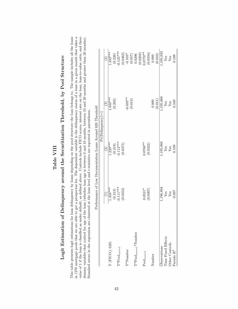
Examination of pool structure reveals several other interesting insights. First, we show that

pools where loans are primarily originated by independent lenders tend to perform better around

the threshold as compared to those where banks primarily originate loans. This corroborates our4These findings are consistent with the review report “Observations on Risk Management Practices during the

Recent Market Turbulence” that was a jointly conducted by seven supervisory agencies around the world: theFrench Banking Commission, the German Federal Financial Supervisory Authority, the Swiss Federal BankingCommission, the U.K. Financial Services Authority, and, in the United States, the Office of the Comptroller ofthe Currency, the Securities and Exchange Commission, and the Federal Reserve. The report assesses a rangeof risk management practices among a sample of major global financial services organizations and analyzes theperformance of eleven major banking and securities firms in the period prior to and during the subprime crisis.

3

earlier results comparing loans originated by banks and independents. More importantly, we find

a positive correlation between number of lenders contributing to pool and the performance of

the pool i.e., higher diversity lowers the default rates. One plausible explanation for this result

is that issuers of pools benchmark the quality of the loans offered by a given lender against

the other lenders and relative performance mitigates the moral hazard problem to some extent

(Gibbons and Murphy 1990). In summary, we find some support for incentives mitigating moral

hazard in both the lenders in the OTD market.

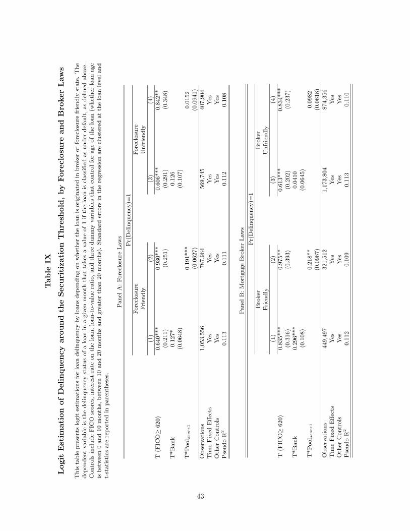
We conclude our analysis by exploiting cross-sectional variations in two state-level laws that

have attracted a lot of attention in recent policy debates related to the OTD market: laws

related to the monitoring of brokers and the ease of foreclosing property. First, we examine the

effect of state broker laws using the database reported in Pahl (2007). We find that stringent

broker regulation helps reduce bad loans of both banks and independent lenders around the

threshold. We view these results as consistent with the importance of incentives in the OTD

market. The reason is that broker compensation is based on commission received from both the

lender and the borrower. Such a compensation structure encourages brokers to maximize the

volume of the loans they originate rather than the quality of their origination. Stringent broker

laws can help align the perverse incentives created by a fee-based structure since most of these

involve surety bonds. This form of regulation, we argue, requires brokers to have a ‘skin in the

game,’ since there is a credible threat of upholding these bonds from mortgage lenders (banks

and independent lenders).

Finally, we analyze the effect of foreclosure laws on the moral hazard problem in the OTD

market. For this purpose, we exploit the cross-sectional variation generated by state foreclosure

laws. States vary by the degree of difficulty in recovering collateral for lenders. The incentives to

screen therefore should be weakest in states where lenders are likely to recover collateral relatively

easily, should the borrower default (following the insights in Manove, Padilla and Pagano 2001).

In the U.S., many states protect borrowers by imposing restrictions on the foreclosure process.

This imposes costs on lenders and therefore should ex-ante lead to more careful screening by

lenders. If, on the other hand, certain states make collateral easy to repossess through creditor-

friendly foreclosure policy, the screening incentives of lenders in these states may be weakened.

To test this, we follow Pence (2003) and classify states as being lender-friendly or not in regards

to foreclosure law. Our results support the view that lender-friendly foreclosure policies distort

incentives and thus aggravate the moral hazard problem in the OTD market.

Our results have several important policy implications. Contrary to popular belief, highly

regulated lenders, banks, defaulted more than independents who faced weaker regulation but

may have been more disciplined by market forces. Thus calls for special regulations and more

supervision of independent lenders may be misplaced. We also find that the moral hazard

4

problem is mitigated to some extent by incentive contracts, as is evident from the structure

of risk managers’ compensation and state-level analysis of brokerage laws. In addition, there

is some evidence that competition among lenders who contributed to a mortgage pool might

help improve the quality of loans originated in that pool. Overall, these results lean towards

suggesting that market forces rather than regulation have been more effective in mitigating

moral hazard in the OTD market.

The rest of the paper is organized as follows. Section II provides a brief overview of securitized

lending in the subprime market and describes the data. Section III discusses the empirical

framework, while Sections IV through VIII present the empirical tests described above. Section

IX concludes.

II Lending in the Subprime Market

II.A Overview

Approximately 60% of U.S. mortgage debt ($3.6 trillion outstanding as of January 2006) is

traded in mortgage-backed securities (MBS), the bulk of which is comprised of agency pass-

through pools – those issued by Freddie Mac, Fannie Mae and Ginnie Mae (Chomsisengphet

and Pennington-Cross 2006). The remainder, approximately $2.1 trillion as of January 2006,

has been bundled and sold as non-agency securities. The two markets are delineated by the

eligibility criteria of loans established by the government-sponsored enterprises (GSEs). Agency

eligibility is generally determined on the basis of loan size and underwriting standards and the

borrower’s creditworthiness.

While the non-agency MBS market (referred to as “subprime” in the paper) is relatively

small as a percentage of all U.S. mortgage debt, it is nevertheless large on an absolute dollar

basis. This market gained momentum in the mid- to late-1990s as total subprime lending (B&C

originations) grew from $65 billion in 1995 to $500 billion in 2005 (Inside B& C lending). As the

securities market grew in size it also grew in importance for originators, as securitization rates

(the ratio of the value of loans securitized divided by the value of loans originated) increased

from less than 30 percent in 1995 to over 80 percent by 2006.

From the borrower’s perspective, the primary distinguishing feature between prime and

subprime loans is that both the up-front and continuing costs are higher for subprime loans.

Up-front costs include application fees, appraisal fees, and other fees associated with originating

a mortgage. The continuing costs include mortgage insurance payments, principle and interest

payments, late fees for delinquent payments, and fees levied by a locality such as property taxes

or special assessments. The price of subprime mortgage loans, most importantly the interest

5

rate, is actively based on the risk associated with the borrower, as measured by the borrower’s

credit score, debt-to-income ratio, and the documentation of income and assets provided at the

time of origination. In addition, the exact pricing may depend on the amount of equity provided

by the borrower (the loan-to-value ratio), the length and size of the loan, the flexibility of the

interest rate (adjustable, fixed, or hybrid), the lien position, the property type and whether

stipulations are made for any prepayment penalties.

II.B Process and Participants

When a borrower approaches a lender for a mortgage loan, either directly or through a mortgage

broker, the lender asks the borrower to fill out a credit application. The lender also obtains the

borrower’s credit report from the three credit bureaus. Part of the background information on

the application and report could be considered “hard” information (e.g., the FICO score of the

borrower), while the rest is “soft” (e.g., a measure of future income stability of the borrower,

how many years of documentation were provided by the borrower, joint income status) in the

sense that it is more difficult to summarize on a legal contract.

The lender expends effort to process the soft and hard information about the borrower and,

based on this assessment, offers a menu of contracts to the borrower (or does not extend a

loan offer). Subsequently, borrowers decide to accept or decline the loan contract offered by the

lender. Once a loan contract has been accepted, the loan can be sold as part of a securitized

pool to investors. The risk associated with investing in the loan pools depends in part on

whether the loans are from the agency or non-agency market. In contrast to “pass-through”

MBSs from the agency market that bear limited credit risk due to implicit guarantees from the

GSEs, MBSs from the subprime market mitigate credit risk for higher tranches mainly through

credit enhancement and over-collateralization.

The key participants in the originate-to-distribute (OTD) chain – brokers and lenders – are

regulated to varying degrees. On the one hand, federally insured depository institutions and their

affiliates (called banks in the paper) which originate, purchase, or distribute are regulated under

federal supervision. In particular, these banks are supervised by the Office of the Comptroller

of the Currency (OCC), Office of Thrift Supervision (OTS), the Federal Reserve, FDIC or some

combination of all four groups assigned to oversee the affiliates of federally insured depository

institutions. On the other hand, mortgage brokers who assist consumers in securing mortgage

products and independent lenders who develop and fund mortgage products have no federal

supervision. These mortgage market participants are subject to uneven degrees of state-level

oversight and in some cases limited or no oversight (see Treasury Blueprint report 2008). Thus,

even though the participants are performing similar origination actions, they are differentially

6

regulated.

Among the bodies that oversee banks, the OCC charters, regulates, and examines all na-

tional banks and federally licensed branches and agencies of non-U.S. banks. It has regulatory

and examination responsibility over national banks and promulgates rules, legal interpretations,

and corporate decisions concerning bank applications, activities, investments, community devel-

opment activities, and other aspects of national bank operations. The OCC’s bank examiners

frequently conduct on-site examinations of national banks and examine bank operations. It

can take various actions against national banks that fail to comply with laws and regulations

or otherwise engage in unsound banking practices, such as remove bank officers and directors

and/or impose monetary fines. The OTS plays a role for federally chartered thrifts similar to

that of the OCC for national banks.

The Federal Reserve System, the independent U.S. central bank, consists of twelve regional

statutorily established Federal Reserve Banks, each of which effectively performs functions of a

central bank for its geographic region. The Federal Reserve has the principal responsibility for

formulating and executing national monetary and credit policy, fulfilled primarily through its

open market operations, reserve requirements for depository institutions, and discount window

lending program. It functions as the primary federal regulator of state member banks, bank

holding companies, U.S. operations of foreign banks, and the foreign activities of member banks.

Finally, the FDIC administers the federal deposit insurance system under the Federal Deposit

Insurance Act. The agency monitors risks to the deposit insurance fund and possesses a wide

range of enforcement powers with respect to insured institutions, including the right to terminate

insurance coverage of any institution engaged in unsafe or unsound practices.

We will examine the performance of loans that are securitized by banks relative to those

securitized by independents to assess the costs and benefits of allowing some market participants

to operate beyond the scope of regulation. It is worth noting that while we will make statements

about regulations at federal (banks) vs. state (independents) level, our tests will not have the

power to determine which federal bodies or specific aspects of regulation or drive our results.

II.C Data

Our primary data are leased from LoanPerformance, who maintain a loan-level database which

provides a detailed perspective on the non-agency securities market. The data includes, as of

December 2006, more than 7,000 active home equity and non-prime loan pools that include more

than 7 million active loans with over $1.6 trillion in outstanding balances. LoanPerformance

7

estimates that, as of 2006, the data covers over 90% of the subprime loans which are securitized.5

The dataset includes information on issuers, broker dealers/deal underwriters, servicers, master

servicers, bond and trust administrators, trustees, and all standard loan application variables.

The borrower’s credit quality is captured by a summary measure called the FICO score.

FICO scores are calculated using various measures of credit history, such as types of credit in use

and amount of outstanding debt, but do not include any information about a borrower’s income

or assets (Fishelson-Holstein 2004). The software used to generate the score from individual

credit reports is licensed by the Fair Isaac Corporation to the three major credit repositories

– TransUnion, Experian, and Equifax. These repositories, in turn, sell FICO scores and credit

reports to lenders and consumers. FICO scores provide a ranking of potential borrowers by

the probability of having some negative credit event in the next two years. Keeping this as a

backdrop, most of our tests of borrower default will examine the default rates up to 24 months

from the time the loan is originated. Nearly all scores are between 500 and 800, with a higher

score implying a lower probability of a negative event. The negative credit events foreshadowed

by the FICO score can be as small as one missed payment or as large as bankruptcy. These

scores have been found to be accurate even for low-income and minority populations.6

Borrower quality can also be gauged by the level of documentation collected by the lender

when taking the loan. The documents collected during the screening process provide historical

and current information about the income and assets of the borrower. Documentation in the

market (and reported in the LoanPerformance database) is categorized as full, limited, or no

documentation. Borrowers with full documentation provide verification of income as well as

assets. Borrowers with limited documentation provide no information about their income but

do provide some information about their assets. “No-documentation” borrowers provide no

information about income or assets, which is a very rare degree of screening lenience on the part

of lenders. In our analysis, we combine limited and no-documentation borrowers and call them

low documentation borrowers. Our results are unchanged if we remove the very small portion

of loans which are no documentation.

There is also information about the property being financed by the borrower, and the purpose5Note that only loans which are securitized are reported in the LoanPerformance database. Communication

with the database provider suggests that the 10% of loans that are not reported are for privacy concerns fromlenders. Importantly for our purpose, the exclusion is not based on any selection criteria that the vendor follows(e.g., loan characteristics or borrower characteristics). Moreover, based on estimates provided by LoanPerfor-mance, the total number of non-agency loans securitized relative to all loans originated has increased from about65% in early 2000 to over 92% since 2004.

6For more information see www.myfico.com; also see Chomsisengphet and Pennington-Cross (2006). An econo-metric study of loan data from the early 1990s by Freddie Mac researchers showed that the predictive power ofFICO scores drops by about 25 percent once one moves to a three-to-five year performance window (Holloway,MacDonald and Straka 1993). FICO scores are still predictive, but do not contribute as much to the default rateprobability equation after the first two years.

8

of the loan. Specifically, we have information on the type of mortgage loan (fixed rate, adjustable

rate, balloon or hybrid), and the loan-to-value ratio (LTV) of the loan, which measures the

amount of the loan expressed as a percentage of the value of the home. Loans are classified

by purpose as either for purchase or refinance, though for convenience we focus exclusively on

loans for home purchases. The reason is that, in contrast to refinance or investor property

markets, the purchase part of the market was considered to be least affected by speculative

motives. We should note that similar rules of thumb and default outcomes exist in the refinance

and investor property markets as well. Information about the geography where the dwelling is

located (zipcode) is also available in the database.

To ensure reasonable comparisons we restrict the loans in our sample to owner-occupied

single-family residences, townhouses, or condominiums, which make up the majority of the

loans in the database. We exclude non-conventional properties, such as those that are FHA

or VA insured or pledged properties, and also omit buy-down mortgages. Alt-A loans are also

excluded because the coverage for these loans in the database is limited. Only those loans with

valid FICO scores are used in our sample. We conduct our analysis for the period January 2001

to December 2006, the period in which the securitization market for subprime mortgages grew

to a meaningful size (Gramlich, 2007).

To conduct our tests, we classify lenders in our sample into banks, thrifts, subsidiaries of

banks/thrifts, and independent lenders. Each loan in the database is linked to an originating

lender. However, it is difficult to directly discern all unique lenders in the database since the

names are sometimes spelled differently and in many cases are abbreviated. We manually

identified the unique lenders from the available names when possible. In order to ensure that we

are able to cover a majority of loans in our sample, we also obtained a list of top 50 lenders (by

origination volume) for each year from 2001 to 2006, previously published by the publication

‘Inside B&C mortgage’. Across years, this yields a list of 105 lenders. Using these lender names

we are able to identify some abbreviated lender names which otherwise we might not have been

able to classify. Subsequently, we use 10-K proxy statements and lender websites (whenever

available) to classify the lenders into two categories – banks which comprise all lenders that are

banks, thrifts, or subsidiaries of banks and thrifts and independents. An example of a bank in

our sample would be Countrywide while Ameriquest is an example of an independent lender.

Our sample consists of 48 banks and 57 independent lenders.

Our tests also employ additional data on the financials of banks, the incentives of CEOs and

risk managers, the structure of the loan pools, and state foreclosure and mortgage broker laws.

Relevant data for these tests is discussed in Sections V, VI and VII.

9

III Framework and Tests

III.A Theoretical Framework and Identification

To understand our empirical methodology, it is useful to first describe the thought experiment

which informs the lenders’ decision-making. When a borrower approaches a lender for a loan –

directly or through a broker – the lender may acquire both hard information (such as a FICO

score) and soft information about the borrower. By soft information we refer to any information

that is not easily documentable or verifiable. This includes, for example, the likelihood that

the borrower’s job may be terminated, or other upcoming expenses not revealed by her current

credit report. It also includes information about the borrower’s income or assets that is costly for

investors to process. Borrowers have types, and both hard and soft information play a valuable

role in screening loan applicants. However, collecting and evaluating soft information is costly.

With securitization the distance between the originator of the loan and the party that bears

the default risk inherent in the loan increases. Because soft information about borrowers is

unverifiable to a third party (as in Stein 2002), the increase in distance may result in lenders

choosing not to collect soft information about borrowers. While lenders are compensated for

the hard information they collect on the borrower, the incentive for lenders to process soft

information critically depends on whether they have to bear the risk of loans they originate.

A lender chooses to incur the cost of acquiring soft information only if the signal provided by

the borrower’s hard information is imprecise or if there is a sufficient chance that lender would

retain the loan on its balance sheet.

The central claim in this paper is that lenders are less likely to expend effort to process

soft information as the ease of securitization increases. We measure the extent of this effort by

examining the performance of loans originated by the lender. In order to make any assessment

about soft information, we condition on the hard information that investors and lenders use to

price the loans. Any residual differences in default rates on either side of the cutoff should then

only be due to the lenders’ screening effort on the soft information dimension.

The challenge in making a causal inference related to securitization and the performance of

loans originated by a lender is the difficulty in isolating differences in loan outcomes independent

of contract and borrower characteristics. First, in any cross-section of loans, those which are

securitized may differ on observable and unobservable risk characteristics from loans which

are kept on the balance sheet (not securitized). Second, in a time-series framework, simply

documenting a positive correlation between securitization rates and defaults is insufficient to

establish a causal relationship. This inference relies on determining the optimal level of defaults

at any given point in time, an impossible econometric exercise. Moreover, this approach ignores

10

macroeconomic trends and policy initiatives which may be independent of lax screening and yet

may induce compositional differences in mortgage borrowers over time.

To circumvent these problems, we first identify a plausibly exogenous change in the ease

of securitization. We do so by exploiting a specific rule of thumb at the FICO score of 620

which makes the securitization of loans more likely if a certain FICO score threshold is attained.

Historically, this score was established as a minimum threshold in the mid-1990’s by Fannie Mae

and Freddie Mac in their guidelines on loan eligibility (Avery et al. 1996). According to Fair

Isaac, “...those agencies [Fannie Mae and Freddie Mac], which buy mortgages from banks and

resell them to investors, have indicated to lenders that any consumer with a FICO score above

620 is good, while consumers below 620 should result in further inquiry from the lender....”7 For

other details on the FICO score securitization cutoff refer to Keys et al. (2008).

We argue that adherence to this cutoff by investors (investment banks, hedge funds), fol-

lowing the advice of GSEs generates an increase in demand for securitized loans which are just

above the credit cutoff relative to loans below this cutoff. In other words, the likelihood of loan

securitization dramatically increases when we move along the FICO distribution from 620− to

620+. This increase is equivalent to the unconditional probability of securitization increasing

as one moves from 620− to 620+. To see this, denote N620+

s and N620−s as the number of loans

securitized at 620+ and 620− respectively. Showing that N620+

s > N620−s is equivalent to showing

N620+sNp

> N620−sNp

, where Np is the number of prospective borrowers at either 620+ or 620−.

As one approaches any FICO score from either side, differences in the characteristics of

borrowers should be random. This implies that the underlying creditworthiness and the demand

for mortgage loans (at a given price) is the same for prospective buyers with a credit score of

620− or 620+. This amounts to saying that the calculation Fair Isaac performs to generate credit

scores has a random error component around any specific score. In addition, the distribution of

the FICO score across the population is smooth, so the number of prospective borrowers around a

given credit score is similar (in the example above, N620+

p ≈ N620+

p = Np). Thus, higher numbers

of securitized loans above the threshold translate directly into a higher unconditional probability

of securitization at 620+. We refer to the difference in these unconditional probabilities as the

differential ease of securitization around the threshold.

Because investors purchase securitized loans based on hard information, our assertion is that

the costs of collecting soft information are internalized by lenders to a greater extent when the7This was reported by Craig Watts, a spokesperson for Fair, Isaac and Company in an interview to the Detroit

Free Press. Similarly, Charles Capone, Jr., a senior Analyst with the Microeconomic and Financial Studies Divisionof the U.S. Congressional Budget Office wrote in “Research Into Mortgage Default and Affordable Housing: APrimer” that for most of the 1990s, the mortgage market viewed a FICO score of 620 as the bottom cutoff of loansthat could be sold to Fannie Mae or Freddie Mac. Also see Freddie Mac, Single-Family Seller/Servicer Guide,Chapter 37, Section 37.6: Using FICO Scores in Underwriting (03/07/01).

11

unconditional probability of securitization is lower. As a result, 620− loans should perform

better as compared to 620+ loans. This difference in default rate on either side of the cutoff,

after controlling for hard information, as argued earlier, should be only due to the impact that

securitization has on lenders’ screening standards. Notably, our assertion of differential screening

by lenders does not rely on knowledge of the proportion of prospective borrowers that applied,

were rejected, or were held on the lenders’ balance sheet. We simply require that lenders’ are

aware that a prospective borrower at 620+ has a higher likelihood of eventual securitization.

Also note that in our assertion, we assume that screening is costly for the lender. The notion is

that collection of information – hard systematic data as well as soft information of the borrower

– requires time and effort by loan officers. This seems to be a reasonable assumption (see Gorton

and Pennacchi, 1995).

The discussion thus far has assumed that there is no explicit manipulation of FICO scores by

the lenders or borrowers. However, both the lender and the borrower may have incentives to do so

if loan contracts or screening differs around the threshold. Our subsequent analysis will confirm

that there are no differences in loan contract terms around the threshold. Any manipulation

that might be occurring due to differential screening around the threshold is consistent with our

hypothesis. For more on the potential role of manipulation, see Keys et al. (2008).

III.B Overview of Tests

Our main tests examine how the differential performance around the threshold varies cross-

sectionally across lenders that are regulated to varying degrees. In particular, we examine how

loans securitized by banks perform relative to those securitized by independents around the

threshold. This is an important test because both banks and independent lenders have been

equally responsible for originating and distributing loans in the subprime market during the

period 2001-2006 (Treasury Blueprint report 2008).

In addition, motivated by theories of banking, we assess how different lender-level char-

acteristics such as the fragility of capital structure and incentives (direct and indirect) might

impact the differences in performance. Finally, as mortgage brokers have become increasingly

important in helping to originate loans in the OTD market, we also assess the effect regulating

these brokers has on the differential quality of the loans around the securitization threshold. We

discuss the economic motivation and implications of these tests in Sections V, VI and VII.

12

IV Descriptive Statistics and Ease of Securitization

IV.A Descriptive Statistics

We start by looking at the descriptive statistics on three dimensions that distinguish a subprime

loan from one in the prime market: FICO scores, loan-to-value ratios and the amount of doc-

umentation asked of the borrower. Our analysis uses more than one million loans across the

period 2001 to 2006. The non-agency securitization market has grown dramatically since 2000,

which is apparent in Panel A of Table I, which shows the number of securitized subprime loans

across years.

The market has witnessed an increase in the number of loans with reduced hard information

in the form of limited or no documentation.8 In our analysis we combine both types of limited-

documentation loans and denote them as low documentation loans. The full documentation

market grew by 445% from 2001 to 2005, while the number of low documentation loans grew by

972%. LTV ratios have gone up over time, as borrowers have put in less and less equity into their

homes when financing loans. Average FICO scores of individuals who access the subprime market

have been increasing over time. The mean FICO score among low documentation borrowers

increased from 627 in 2001 to 654 in 2006. This increase in average FICO scores is consistent

with the rule of thumb leading to a larger expansion of the market above the 620 threshold.

Average LTV ratios are lower and FICO scores higher for low documentation as compared to

the full documentation sample. This likely reflects the additional uncertainty lenders have about

the quality of low documentation borrowers.

Low documentation loans are on average larger and given to borrowers with higher credit

scores than loans where full information on income and assets are provided. However, the two

groups of loans have similar contract terms such as interest rates, loan-to-value ratios, prepay-

ment penalties, and whether the interest rate is adjustable or fixed. Our analysis below focuses

first on the low documentation segment of the market, and we explore the full documentation

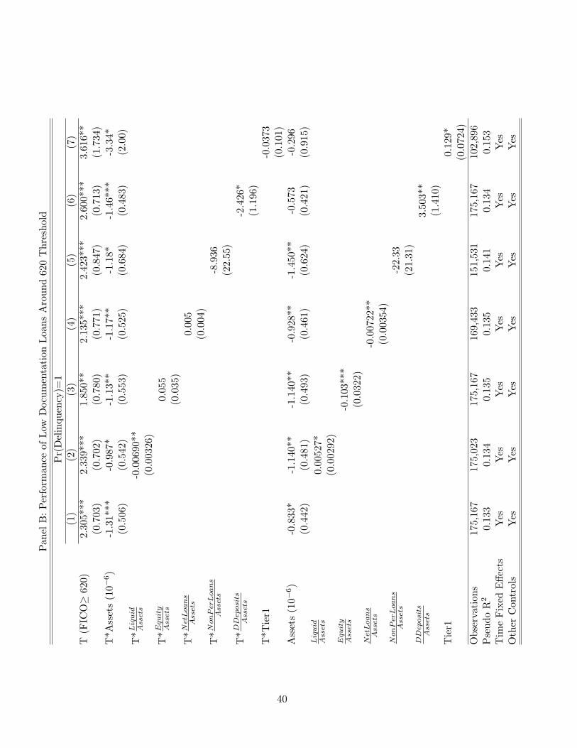
market in Section VIII.

Panels B and C of Table I compares the attributes of the sample based on whether the

loan was originated by banks and independent lenders. Independent lenders in the subprime

market originate a majority of the overall loans (roughly 1.5 million out of 2 million in our

sample). In this regard, our data is consistent with the work of Vickrey (2007), who uses

the Mortgage Interest Rate Survey (MIRS) and finds a similar pattern of finance companies

originating the majority of loans. Both the independents and the banks show similar trends

to the overall sample. In the low documentation market, Bank LTV ratios were essentially flat8Limited documentation provides no information about income but does provide some information about assets

while a no-documentation loan provides information about neither income nor assets.

13

at 87 since 2003, and the average FICO score for bank-originated loans has ranged from 657

to 667. Independents have had slightly lower LTV ratios (implying that they require a larger

down payment), between 84 and 86, while catering to slightly less creditworthy, but overall very

similar borrowers, with FICO scores ranging from 654 to 658.

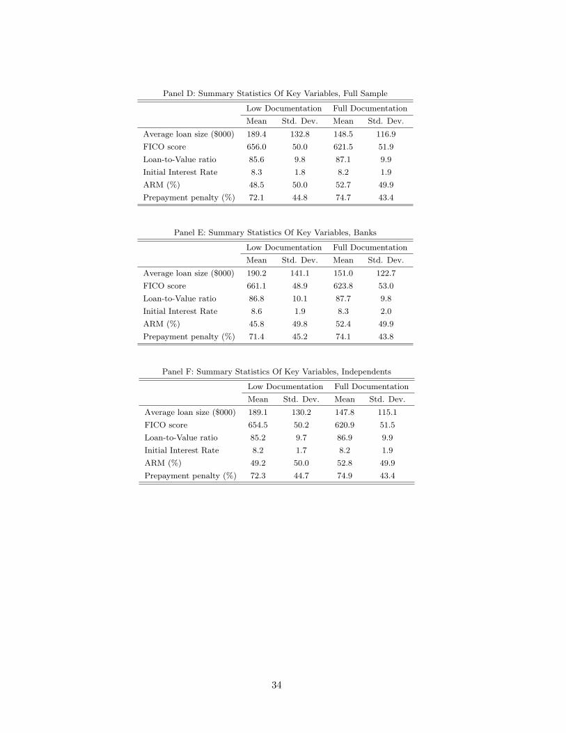
On average, the characteristics of the loans originated by banks and independents are very

similar as can be observed in Panels E and F. The average size of low documentation loans are

$190,200 for banks and $189,100 for independents, and the average LTV ratios are 87 and 85,

respectively. Although bank borrowers are slightly more creditworthy on average (FICO of 661

vs. 654), they nonetheless pay a slightly higher interest rate (8.6% vs. 8.2%), most likely due to

the differences in LTV ratios. Because of the variation in LTV and interest rates, it is important

to include these variables when estimating the performance of the loans around the threshold

since differences in loan terms could possibly explain the differences we observe in the outcomes

of loans originated by banks as compared to independents.

IV.B Variation in the Ease of Securitization Around 620

We first present results that show that large differences exist in the number of low documentation

loans that are securitized around the credit threshold we described earlier. As mentioned in

Section III, the rule of thumb in the lending market impacts the ease of securitization around

the credit score of 620. We therefore expect to see a substantial increase in the number of loans

just above this credit threshold as compared to number of loans just below this threshold. In

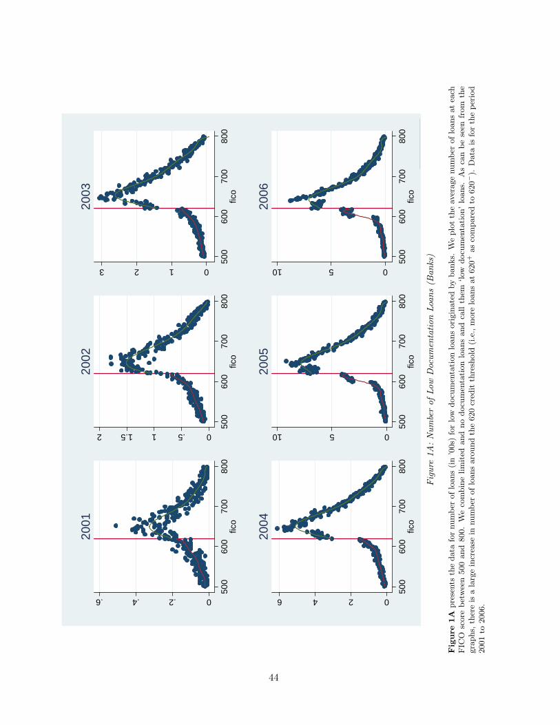
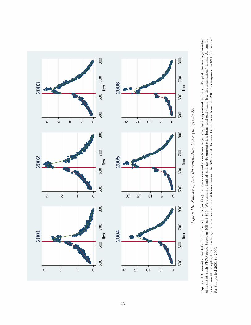
order to examine this, we start by plotting the number of loans at each FICO score for the

two types of lenders for the two documentation categories around the credit cutoff of 620 across

years starting with 2001 and ending in 2006.

From Figure 1A, it is clear that the number of loans see roughly a 100% jump in 2004 for

low documentation loans originated by banks around the credit score of 620 – i.e., there are

twice as many loans securitized at 620+ as compared to loans securitized at 620−. Clearly,

this is consistent with the hypothesis that the ease of securitization is higher at 620+ than at

scores just below this credit cutoff. Similarly, Figure 1B shows the number of loans originated

by independent lenders. There is a 60% jump in the number of loans in 2004, and a more than

100% jump in 2003 and 2005. We do not find any such jump for full documentation loans at

FICO of 620.9 Given this evidence, we focus on the 620 credit threshold for low documentation

loans as the point where the ease of securitization changes discontinuously.

To formally estimate the magnitude of jumps in the number of loans, we collapse the data9We elaborate more on full documentation loans in Section VIII.

14

on each FICO score (500-800) i, and estimate equations of the form:

Yi = α + βTi + θf(FICO(i)) + δTi ∗ f(FICO(i)) + εi , (1)

where Yi is the number of loans at FICO score i, Ti is an indicator which takes a value of 1 at

FICO ≥ 620 and a value of 0 if FICO < 620 and εi is a mean-zero error term. f(FICO) and

T ∗ f(FICO) are flexible seventh-order polynomials, with the goal of these functions being to

fit the smoothed curves on either side of the cutoff as closely to the data presented in the figures

as possible.10 f(FICO) is estimated from 620− to the left, and T ∗ f(FICO) is estimated from

620+ to the right. The magnitude of the discontinuity, β, is estimated by the difference in these

two smoothed functions evaluated at the cutoff. The techniques is similar to one used in the

literature on regression discontinuity (e.g., see DiNardo and Lee, 2004).

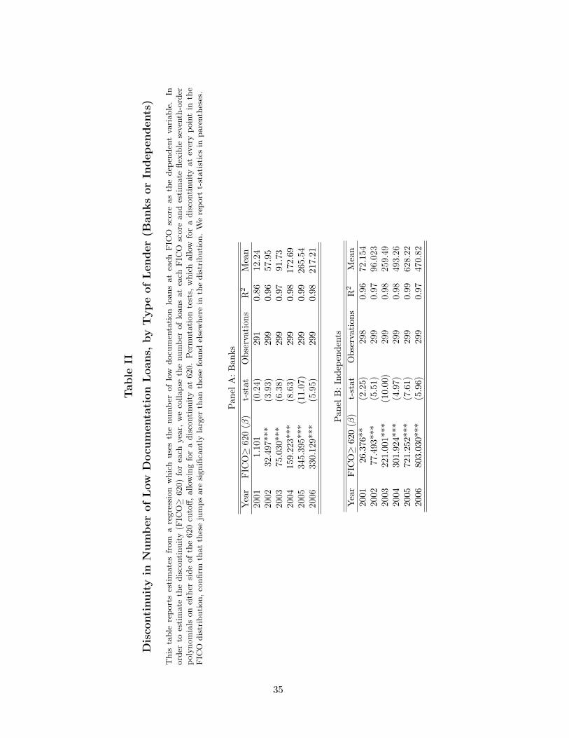
As reported in Table II, we find that low documentation loans see a dramatic increase above

the credit threshold of 620 for both banks (Panel A) and independents (Panel B). In particular,

the coefficient estimate (β) is significant at the 1% level for 2002-2006 vintages of loans, and

is on average around 100% (from 73 to 193%) higher for 620+ as compared to 620− for loans

during the sample period. For instance, in 2003, the estimated discontinuity for banks in Panel

A is 75. The mean average number of low documentation loans originated by banks at a FICO

score for 2003 is 92. The ratio is around 82%.

In results not shown, we conducted permutation tests (or “randomization” tests), where we

varied the location of the discontinuity (Ti) across the range of all possible FICO scores and

re-estimated equation (1). Although there are other gaps in the distribution in other locations in

various years, the estimates at 620 for low documentation are outliers relative to the estimated

jumps at other locations in the distribution. In summary, if the underlying creditworthiness

and the demand for mortgage loans (at a given price) is the same for potential buyers with a

credit score of 620− or 620+, as the credit bureaus claim, this result confirms that it is easier to

securitize loans above the FICO threshold for both types of lenders.

IV.C Hard Information Variables Around 620

Before examining the subsequent performance of loans originated around the credit threshold,

we first test if there are any differences in hard information – either in terms of contract terms or

other borrower characteristics – around this threshold. Although we control for these differences

when we evaluate the performance of loans, it is insightful to examine whether borrower and10We have also estimated these functions of the FICO score using 3rd order and 5th order polynomials in FICO,

as well as relaxing parametric assumptions and estimating using local linear regression. The estimates throughoutare not sensitive to the specification of these functions.

15

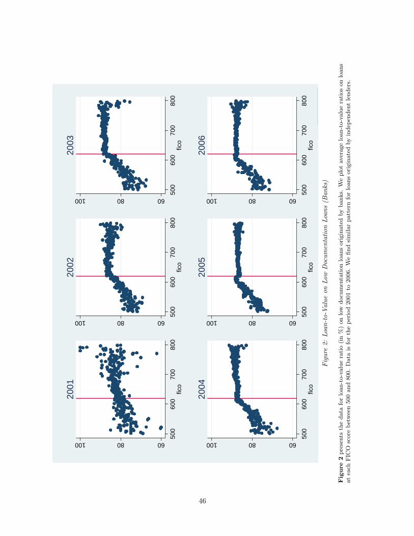
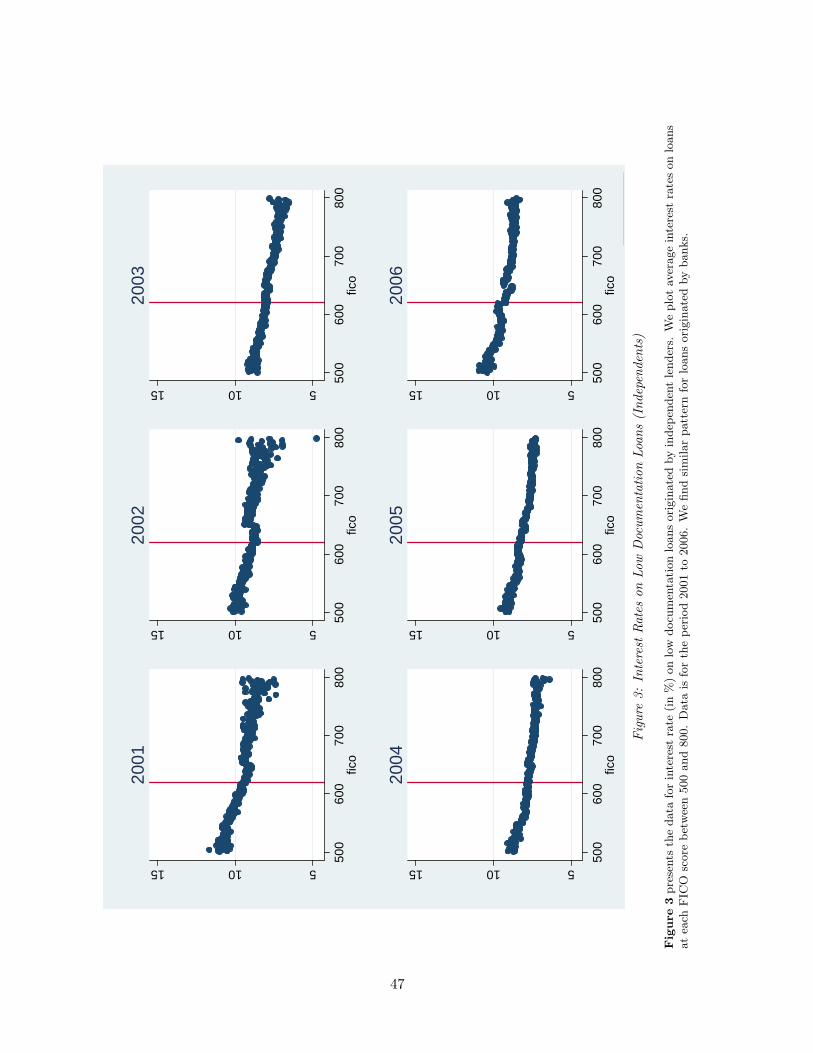
contract terms also systematically differ around the credit threshold. We start by examining

the contract terms – LTV and interest rates – around the credit threshold. To get a sense

of the data, we show the distribution of LTV and interest rates on loan terms offered on low

documentation loans across the FICO spectrum for banks and independent lenders in Figures 2

and 3 respectively. As is apparent from the graphs, we find these loan terms to be very similar

– there are no differences in contract terms for low documentation loans above and below the

620 credit score.

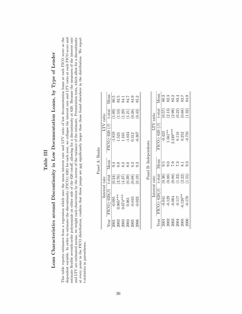
We test this formally using the regression-discontinuity approach equivalent to equation

(1), replacing the dependent variable, Yi, with contract terms (loan-to-value ratios and interest

rates) and present the results in Table III. Our results suggest that there is no discernable

differences in loan terms around the credit threshold for banks and independents. The table

shows that the interest rates (Panel A) and loan-to-value ratios (Panel B) are smooth through

the 620 FICO score for low documentation loans originated by banks and independents. This

confirms the patterns we saw earlier in Figures 2 and 3. In the few cases where the differences are

significantly different from zero, they are economically very small. More specifically, permutation

tests which allow for the location of the discontinuity Ti to occur at each possible FICO score,

confirmed that the estimates at 620 are within the range of other jump estimates across the

spectrum of FICO scores (results not shown). This is also apparent if we take a few examples.

For instance, for low-documentation loans originated in 2006, the average loan-to-value ratio

across the collapsed FICO spectrum for banks is 85.2%, whereas our estimated discontinuity

is only -0.31%, a 0.36% difference. Similarly for the interest rate, for low-documentation loans

originated by independents in 2005, the average interest rate is 8.1%, and the difference on either

side of the credit score cutoff is only about -0.13%, a 1.6% difference.11

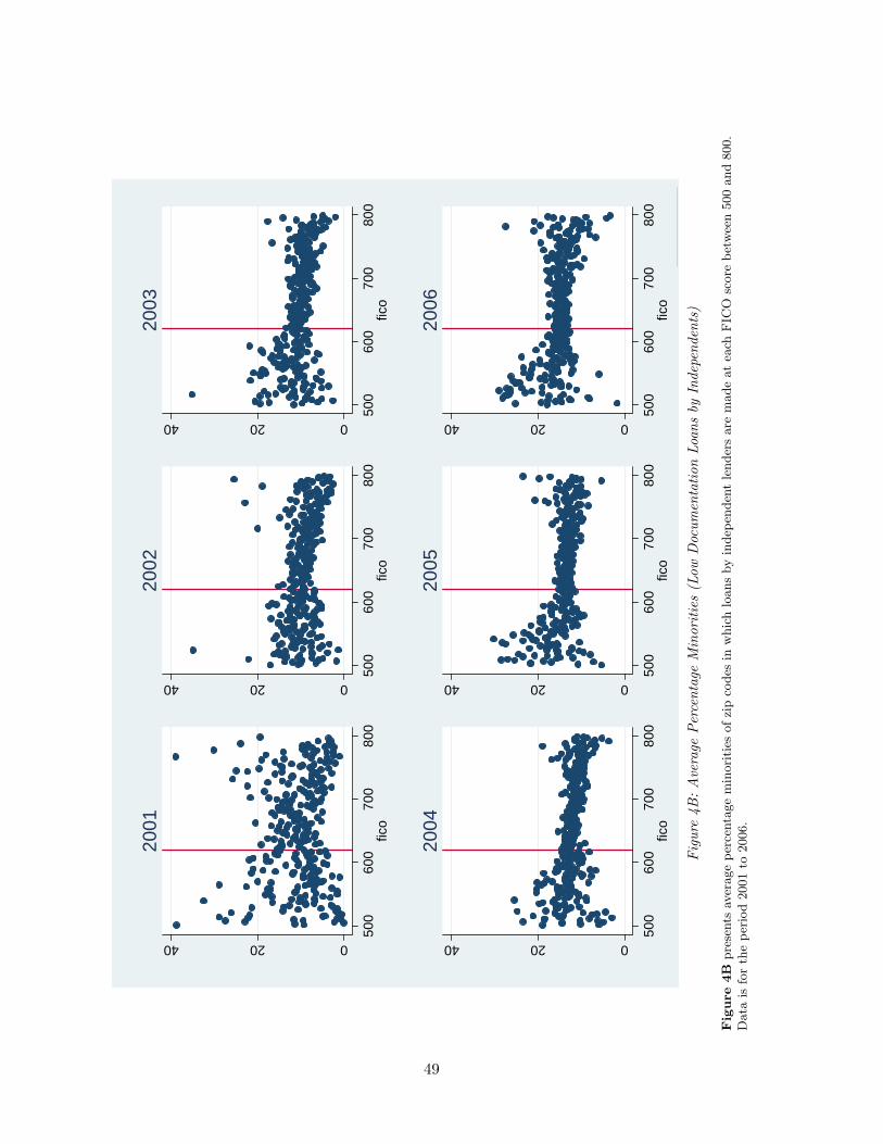
Similarly, if loans are originated in different locations or to different types of borrowers on

either side of the threshold, that could potentially explain differences in loan performance. To

evaluate this conjecture, we examine whether the characteristics of borrowers differ systemat-

ically around the credit threshold. To do so, we look at the distribution of the population of

borrowers across the FICO spectrum for low documentation loans. The data on borrower de-

mographics comes from Census 2000 and is at the zip code level. Of course, since the census

data is at the zip code level, we are to some extent smoothing our distributions. Nevertheless,

we next examine how various zip code level borrower characteristics vary around the threshold.

Figures 4A and 4B show that the average percent minorities of the zip codes of borrowers

around the credit thresholds look very similar for low documentation loans originated by both

banks and independents. We plotted similar distributions for median household income residing11Similar tests (not shown) for whether or not the loan is ARM, FRM or interest only/balloon reveal qualita-

tively identical conclusions.

16

in the zip code, and average house value in the zip code across the FICO spectrum (unreported)

and again find no differences around the credit threshold. We formally estimate any differences

in the average percent of African-American households in the zip code where the loans are

originated for borrowers with credit scores just above and below the 620 threshold using equation

(1). Consistent with the patterns in the figures, we find no differences in borrower demographic

characteristics around the credit score threshold (unreported). For instance, we find that for

low-documentation loans originated in 2005 by banks, the median average percent minority is

16% and the estimated discontinuity around the cutoff is just 0.3%. Similarly small differences

(confirmed by permutation tests) are observed for median household income and household value

of the zipcode where the dwelling is located.

While the results above confirm that there are no differences in contract terms and borrower

demographics around the threshold for both banks and independents, these types of “hard

information” could meaningfully vary across banks and independent lenders below and above

the threshold. If so, this could also explain any differences in performance across the two types

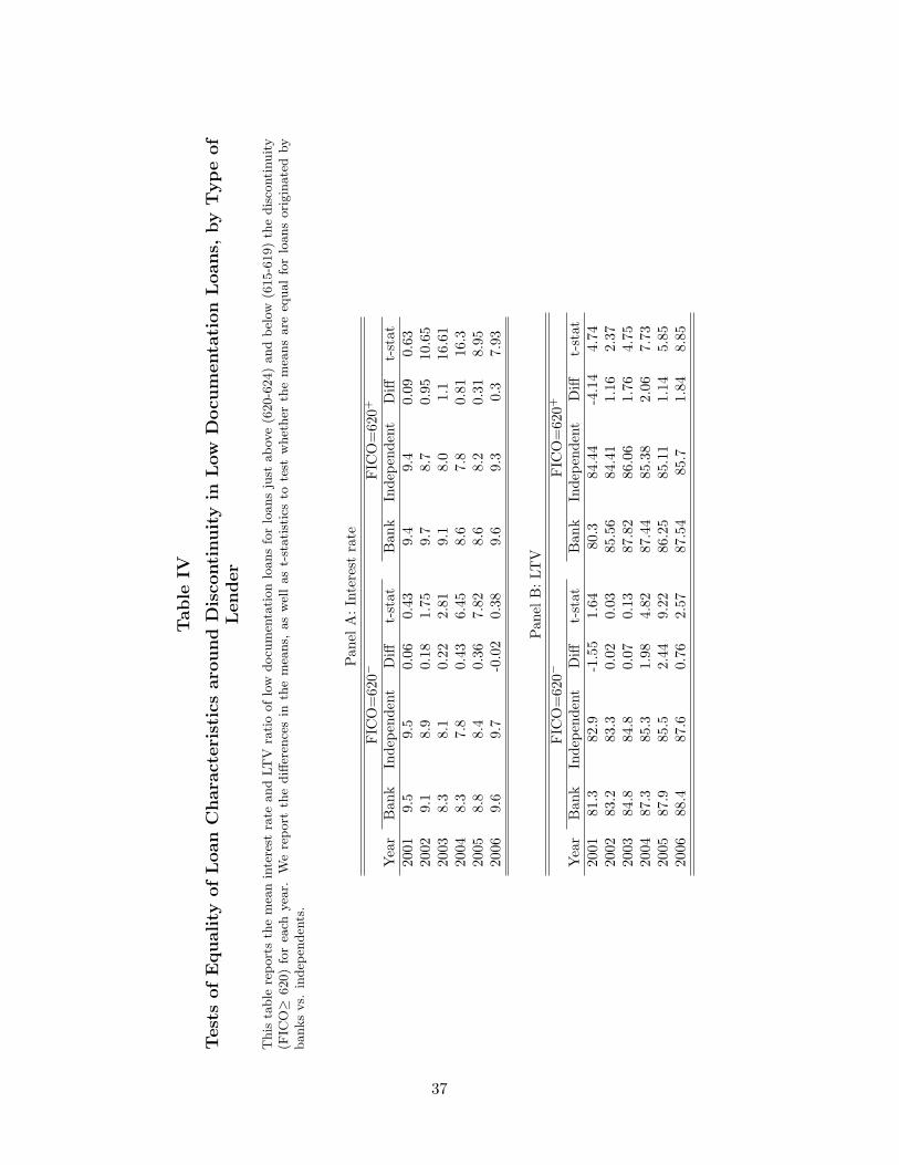
of lenders. To examine this, we compare the attributes of loans just around the credit threshold

(FICO=620) in Table IV. As can be seen, banks charged higher interest rates than independents,

possibly to compensate for higher LTV ratios. Just below 620 (615-619), banks charged 20 basis

points on average higher interest rates than independents, with significant differences (based on

a simple t-test comparison) in 2003-2005. Just above 620, with FICO scores in the range of

620-624, differences are even larger, with a gap of 60 basis points, and significant differences in

2002-2006.

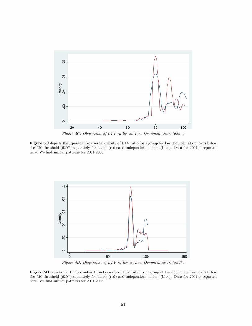
The higher interest rates charged by banks are offset by requiring slightly smaller down-

payments, which results in higher loan-to-value ratios. For those loans made to borrowers with

credit scores just below the threshold, from 2002 onwards the average LTV is one percentage

point higher for banks than independents. These differences are statistically different in 2004-

2006. And just as the gap in interest rates was larger above the threshold, the difference in LTV

ratios is larger above 620 as well. From 2002-2006, the average difference was 1.6 percentage

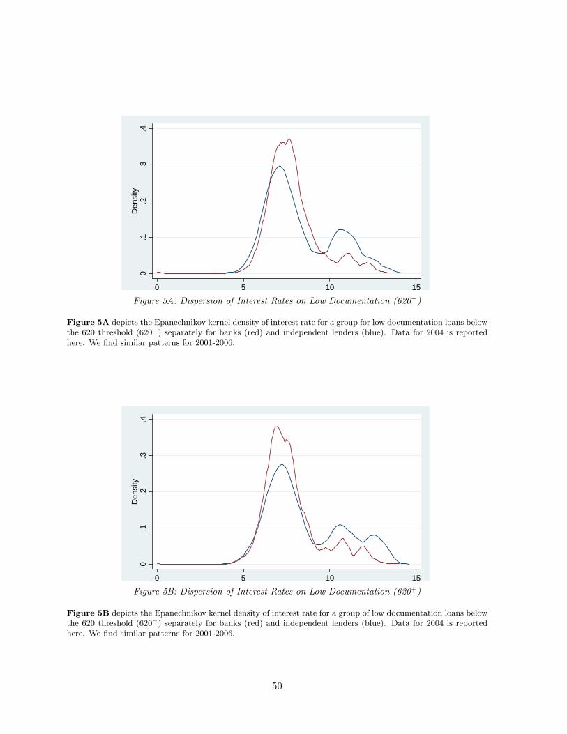
points, and statistically different from zero in all years. We observe same patterns when we plot

distributions of interest rates and LTV below and above the threshold for banks and independents

in Figures 5A and 5B (interest rates) and 5C and 5D (LTV ratios). These differences suggest that

banks are willing to take on slightly higher risks but charge a higher interest rate to compensate

them for doing so. This analysis suggests that our performance regressions should allow for

contract terms to affect loan defaults across banks and independents. We return to this issue in

Section V.

17

V Performance of Loans

We now focus on the performance of the loans that are originated close to the credit score

threshold for both banks and independent lenders. As elaborated earlier, we will control for all

hard information variables that are available to investors. Consequently, any difference in the

performance of the loans above and below the credit threshold can be attributed to differences

in unobservable soft information about the loans.

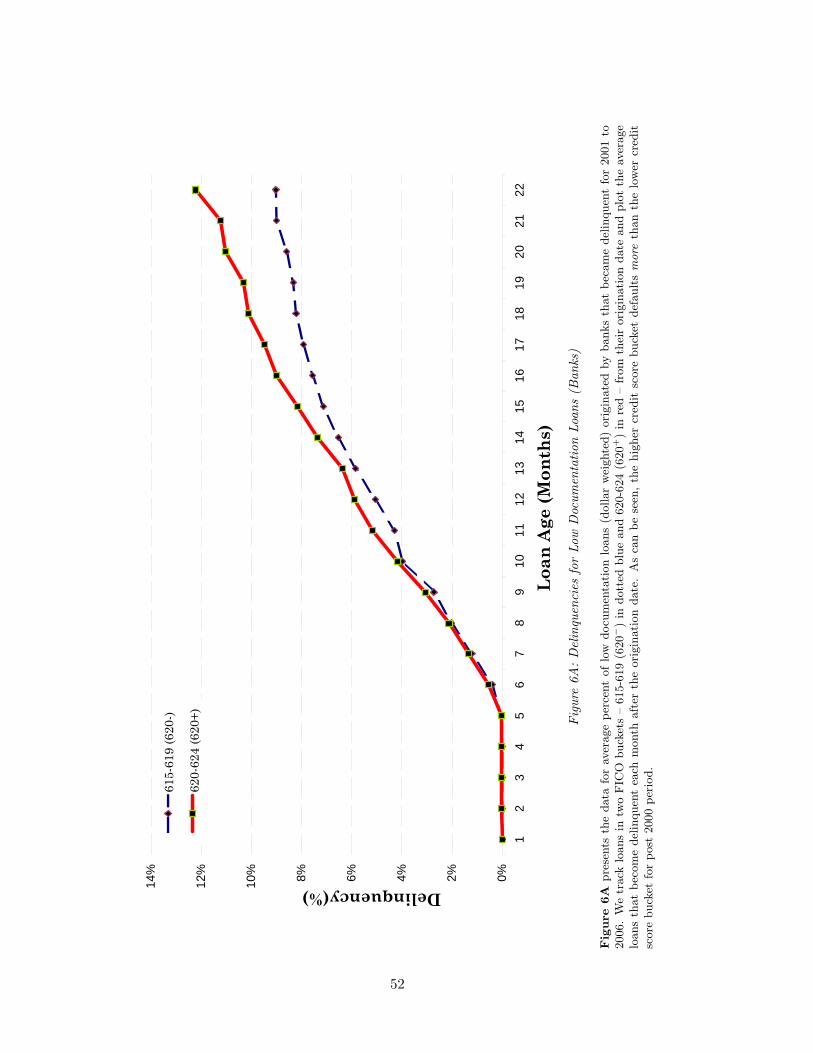
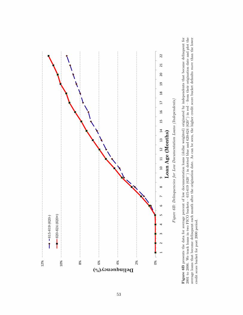
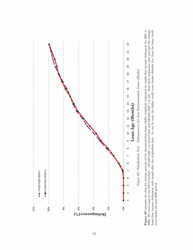
In Figures 6A and 6B, we show how delinquency rates of 620+ and 620− for low documenta-

tion loans evolve over the age of loans originated by banks and independent lenders respectively.

Specifically, we plot the dollar-weighted fraction of loans defaulted up to two years from the

time of origination, with the fraction calculated as the dollar amount of unpaid loans in default

divided by the total dollar amount originated in the same cohort. A loan is classified as under

default if any of the conditions is true: (a) payments on the loan are 60+ days late; (b) the

loan is in foreclosure; or (c) the loan is real estate owned (REO), i.e. the bank has re-taken

possession of the home.12

As can be seen from the figures, delinquency rates are higher for loans above the threshold

for both types of lenders. The differences between delinquency rates of 620+ and 620− loans

begin around four months after the loans have been originated and persist up to two years. For

loans originated by independent lenders, those with a credit score of 620− are about 20% less

likely to default after two years as compared to loans of credit score 620+ for the post-2000

period. Interestingly, the magnitudes are significantly larger for loans originated by banks (28%

vs 20% for independent lenders). As a counterfactual test, we plot delinquency rates around

FICO score of 630. Figure 6C and 6D plot the dollar-weighted fraction of loans defaulting for

banks and independent lenders respectively at this potential threshold. The plots clearly show

that the patterns shown earlier are not observed at score of 630. In fact, for both type of lenders

loans with higher FICO score (630+) default lower than (630−) as should be the case given the

expected negative relationship between FICO score and default.

Next, we examine the differences in performance of each unweighted loan around the thresh-

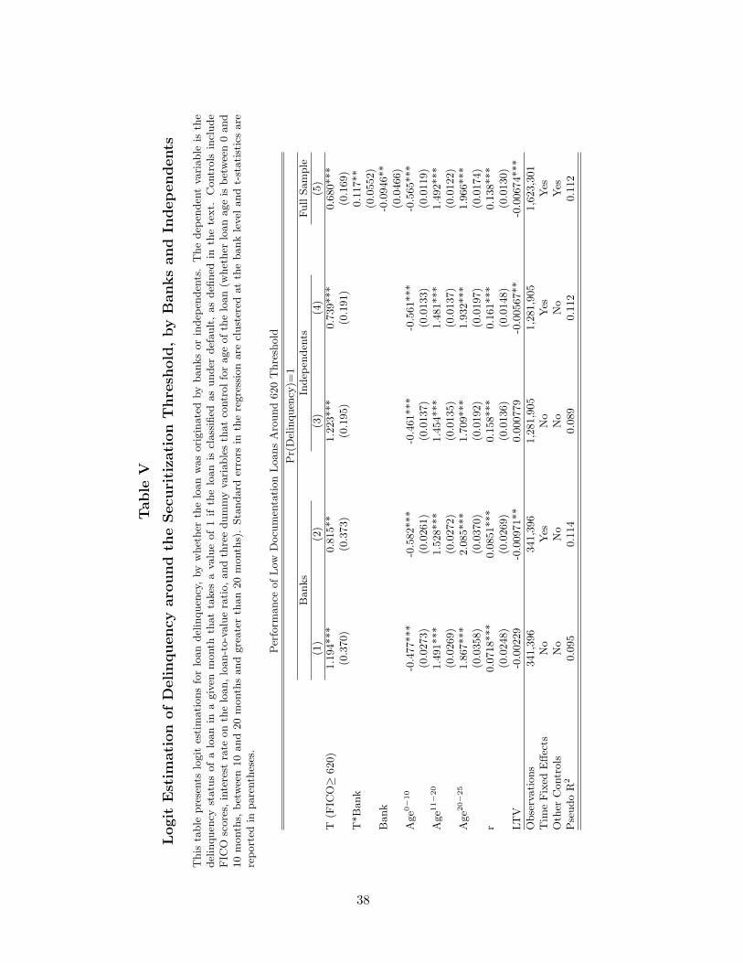
old using variants of the following logit regression:

Yikt = Φ(

α + β1Tit + β2Tit ∗Bankit + β3Bankit + γ1Xikt + δ1Tit ∗Xikt + µt + εikt

). (2)

The dependent variable is an indicator variable (Delinquency) for loan i originated in year t

that takes a value of 1 if the loan is classified as under default in month k after origination12Using data from LoanPerformance, various industry reports find that about 80% of the 60+ loans roll over

to 90+ and another 90% roll over from 90+ to foreclosure in the subprime market. Our results are invariant touse of other definitions of delinquency.

18

as defined above. We drop the loan from the regression once it is paid out after reaching the

REO state. T takes the value 1 if FICO is between 620 and 624, and 0 if it is between 615

and 619 for low documentation loans, thus restricting the analysis to the immediate vicinity of

the cutoffs. Banki takes a value 1 if the loan is originated by a bank and 0 if it is originated

by an independent lender. Controls include FICO scores, the interest rate on the loan, loan-to-

value ratio, borrower demographic variables, and interaction of these variables with T . We also

include a dummy variable for the type of loan (adjustable or fixed rate mortgage) and control

for age of the loan by including three dummy variables – that take a value of 1 if the month since

origination is between 0-10, 11-20 and more than 20 months respectively. Year of origination

fixed effects (µt) are included in the estimation and standard errors are clustered at the loan

level.

We report the logit coefficients in Table V. In the first column we estimate the regression

only for banks and find that β1 is positive and significant. This result is robust to including

time fixed effects as is shown in column (2). Consistent with Figure 6A, estimates in column (2)

suggest that for banks 620+ loans default 15% more than 620− loans (about 0.8% in absolute

terms over mean of about 5.5%). The next two columns in the table repeat the same tests for

independent lenders and find results that are similar in nature, though smaller in magnitude,

for independent lenders.

Why would the independent lenders differentially screen if they are able to sell most of

their mortgages? Our premise is that loans below the threshold are more difficult to securitize.

Consequently, even independent lenders will have incentive to screen these loans more intensively

since these loans are less liquid. In fact, as we argue below, the incentives of these lenders to

screen will be greater than banks since they are very thinly capitalized. Overall, the results in

the first four columns of Table V suggest that loans above the credit threshold which are easier

to securitize default more severely as compared to loans below the threshold for both banks and

independents.

To compare magnitudes across the two types of lenders, we estimate the complete equation

(2) in column (5). The results confirm what separate regressions for banks and independent

lenders had shown – relative to loans above the threshold that are originated by independents,

those originated by banks default more than loans below the threshold, i.e, β1 > 0 and β2 > 0.

The difference is large and of the order of about 10% (about 0.5% in absolute terms over mean

of about 5%). Notably these differences are not on account of differences in contracts that these

lenders offer borrowers since we directly control for these contractual terms in the regression.

How should we interpret these results? One way of interpreting this result is that perhaps

federal supervision of banks is not effective in reducing moral hazard in the OTD market. This

could be – as the Treasury Blueprint (2008) also notes – a case of bank’s mortgage origination

19

activity not being supervised, despite having four entities monitoring other activities of the bank.

In contrast, independent lenders only originate mortgages and as a result their balance sheets

are less complex than banks, perhaps making supervision of their activities easier for regulators.

However, these lenders are lightly supervised at the state level and this casts doubt on regulation

per se resulting in better performance of the loans originated by independent lenders.

If we believe that supervision is not the source this difference in performance, what could

be the reason that loans originated by independent lenders perform better than banks? There

could be at least two other plausible reasons. The first reason could be that banks may screen

loans like independent lenders and then strategically hold on to better loans on their balance

sheets. On the other hand, independent lenders, given their limited equity capital, cannot keep

a portfolio of loans on their books and have limited motive for strategically selling to investors.

Consequently, one would see worse performance on loans that are securitized by banks relative to

those securitized by independents. Unless reputation concerns prevent banks from such strategic

adverse selection (Gorton and Souleles, 2005), this could be a plausible channel. However, note

that adverse selection should be more severe below the 620 threshold since banks have more

leeway in choosing which loans to sell below the threshold.13 As a result if adverse selection was

driving these differences, we should have found that 620− loans originated by banks should have

done worse relative to 620+. However, this is not the case.

An alternative explanation, and one that seems more plausible, could stem from the fragility

of independent lenders’ capital structure relative to those of banks. In contrast to banks, these

lenders finance their operations entirely out of short-term warehouse lines of credit, have limited

equity capital, and have no deposit base to absorb losses on loans that they originate (Gramlich,

2007). Consequently, the ex-post threat of withdrawal of funds might reduce ex ante moral

hazard by these lenders (Calomiris and Kahn 1991; Diamond and Rajan 2003). Note, however,

that while this argument explains why loans originated by independent lenders’ perform better

above the threshold than banks, it does not fully resolve the moral hazard problem of securiti-

zation, since the loans originated by independent lenders do perform significantly worse above

the threshold than below it.

V.A Understanding Bank Behavior and Securitization

In this section we examine the cross-sectional relationship between the attributes of banks and

the types of loans they originate around the 620 threshold. To do so, we collect financial

information of all the largest originating banks in our sample. We obtain banks’ financial data

from Bankscope, a Bureau van Dijk Database, which contains financial information on banks,13This follows from the fact that there is equal borrower demand for loans around the 620 FICO threshold, and

we observe far fewer loans securitized below 620, so banks can be more selective in choosing which loans to sell.

20

including balance sheet and income statement data. Since Bankscope does not cover all banks,

we restrict our attention to the banks that were available in the LoanPerformance database and

we obtain data for the fiscal years 2001-2006. We are able to get information on 37 banks out

of the 48 banks in our sample.

Before examining the performance of loans originated by this subset of banks, we quickly

examine whether it is true that low documentation loans are easier to securitize above the 620

threshold in this subset. In results not shown, we find that the ease of securitization result holds

for this subset of banks as well. The magnitudes of the jump on average are very similar to

what we observed for the entire sample of banks (Table II). The pooled estimate is 489 with a

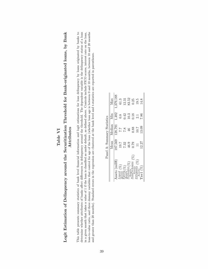
t-statistic of 3.6 (more than 100% jump relative to mean number of loans). In Panel A of Table

VI we present the summary statistics of various bank level characteristics that we use in our

analysis: total assets (Assets), liquid assets-to-assets ratio (LiquidAssets), the equity-to-assets ratio

(EquityAssets ), net loans to assets (NetLoans

Assets ), non-performing loans to assets (NonPerLoansAssets ), demand

deposits to assets (DDepositsAssets ) and Tier-1 capital ratio (Tier1). As can be observed, despite the

small sample, we do have significant variation in almost all of these variables (except Tier-1

capital).

We then use the following logit model to explain the differences in the performance of each

unweighted loan around the threshold only for banks with financial information:

Yikt = Φ(

α + β1Tit + β2Tit ∗Gibt + γ1Xikt + +δ1Tit ∗Xikt + µt + εikt

), (3)

where Gibt is the characteristic of the bank b that originates loan i in year t.14

We start by examining how the performance of loans around the threshold varies with the

size of the bank. To do so we include Tit ∗ Assetsibt in the regression specification. As is

indicated in Panel B of Table VI, we find that larger banks originate loans that do better

around the threshold. There could be several interpretations of this result and we hold off on

discussing the results after we examine other characteristics of banks that might matter. We

next iteratively include other bank level characteristics – LiquidAssets ,

EquityAssets , NetLoans

Assets , NonPerLoansAssets ,

DDepositsAssets and Tier1. As indicated in columns (2) to (7), the size results survive even after

adding these controls. In addition, columns (2) and (6) indicate that banks with more liquid

assets and more demand deposits tend to originate better loans around the threshold. The

effects that we document are economically significant as well. For instance, a bank that is a half

standard deviation larger than a mean bank in the sample originates loans almost as good as

independents. Similarly, banks with two-third standard deviation more liquid assets above the

mean originate loans that are as good as independents.14Standard errors are clustered to allow for unspecified correlation across loans originated by the same bank.

21

There could be several interpretations of these results. First, more reputable banks are likely

to have larger assets, more liquid assets and more demand deposits. This is true in the sample

for instance of Bank of America. In the sample, the correlation between assets and liquid assets

to assets is 0.35 and between assets and demand deposits to assets is 0.51. It is therefore not

surprising that loans of these banks perform better above the threshold. The result for liquid

assets again suggests that healthier banks, who also tend to be larger and reputable, are the

ones who originate better loans above the threshold. In addition, since large banks can attract

demand deposits relatively easily, they are less reliant on securitized markets to free-up capital

for other investment projects (Loutskina and Strahan, 2007). Consequently, for these banks

the liquidity differentials around the threshold are not as large and as a result the screening

incentives are not affected as much.

It is also perhaps surprising that Tier-1 capital by itself does not affect the results. It has

been argued in the literature that imposing capital requirements makes banks more disciplined

since the banks have to put in equity capital for any risky bet they take. In similar vein, banks

that are capital constrained could have lower screening incentives as their incentives to gamble

for resurrection increase (Thakor, 1996). Both these arguments suggest that banks with higher

Tier-1 capital should be originating better OTD loans above the threshold. One reason that we

do not find these results could be that there is little variation in Tier-1 capital across banks in

our sample (Tier-1 capital goes from 7.86 to 14.60). As a result, we are not able to speak as

directly to the literature on capital requirements on banks as we might like.

With regard to the discussion of capital structure fragility in the earlier section, the presence

of demand deposits likely has positive incentive effects on banks. It can be perhaps argued that

demand depositors can ex ante control the risk taking activities of a bank because they make

the capital structure of the bank fragile (Calomiris and Kahn 1991; and Diamond and Rajan

2003). However, it is not obvious if this channel is influencing the results we observe. Banks also

have deposit insurance which mitigates this fragility since the threat of a run is blunted to some

degree. Furthermore, even if the insurance does not fully mitigate this threat, it is difficult to

isolate if all the effects are in fact driven by reputable and large banks also having more demand

deposits.

Overall, the evidence in this section suggests that banks who are large, are more liquid and

have more demand deposits tend to originate better loans above the FICO threshold. The result

is consistent with the interpretation that reputable banks are less reliant on the securitization

market to free-up capital. As a result the liquidity differentials around the credit score threshold

are not large enough for these banks to engage in differential screening.

22

VI Role of Incentives

VI.A Internal Incentives

Did the incentives of management inside the bank have any impact on the quality of loans

originated by banks? Rajan (2008) argues that the incentives of financial market participants

may have been a significant contributing factor to this crisis. In a similar vein, Stein (2008)

argues that “If CEOs with high-powered incentives can’t control risk-taking, what hope do

regulators have?” To assess this speculative arguments in further detail, we hand-collected

data on executive compensation from the Securities and Exchange Commission (SEC) proxy

statements.15 Schedule 14-A proxy statement requires firms to disclose compensation, among

other information, paid to the chief executive officer, to the chief financial officer and to other

most highly compensated executive officers of the company. This information is presented in the

Summary Compensation Table of the proxy statement which provides a comprehensive overview

of a company’s executive pay practices in a consistent format for all the companies. It groups

the executive compensation in three main components: the annual compensation component

(salary, bonus and other annual compensation), the long-term compensation component (awards

and payouts) and the component including all other compensation. We obtain the executive

compensation data for the fiscal years 2001-2006. Overall, we are able to collect compensation

and financial information on 37 lenders with 18 of these lenders being banks and 19 being

independent lenders.

There is significant variation in the total compensation of CEOs. For instance, the total

compensation that the CEOs get paid ranges from $ 270,000 to $ 29 million (average of about

$ 7 million). We also report total compensation of the risk manager in the firm. We are able to

identify the designation of the manager from the Schedule 14-A proxy filings. Similar to CEOs,

there is variation in compensation of risk managers as well. In the sample total compensation

of risk managers ranges from $ 150,000 to $ 16 million (average of about $ 3.5 million).

To formally examine the role of incentives, we estimate equation(3) and include Tit∗Compoibt,

where Compoibt is total compensation of officer O in bank b that originates loan i in year t. We

include Tit ∗ Assetsibt since size of the bank was shown above to be an important predictor of

performance differences around the threshold. Note that the correlation between Tit ∗Bankit ∗Compo

ibt and Tit ∗ Compoibt is about 90%. As a result, we only include one of these variables in

our estimation. This collinearity limits our ability to make statements about differential effects

of compensation across banks and independent lenders.

The results from this specification are reported in Table VII. As column (1) indicates, CEOs’15Note that the bank call report does not provide information on the incentive-based compensation of banks.

23

total compensation per se does not affect the performance of loans around the threshold for banks

or independent lenders. In the next column we add the risk manager’s compensation instead

of the CEO’s total compensation and find that risk manager’s compensation does improve the

quality of loans that are originated around the threshold. This result also is significant when

we include both CEO’s and risk manager’s compensation together in column (3). Why does

risk manager’s compensation matter while that of CEOs does not? Perhaps these are banks

and independent lenders where risk manager is powerful enough to control the firm’s risk-taking

behavior.

To examine this conjecture, we next construct a variable following Bebchuk, Cremers and

Peyer (2008), Centralityrisk, as the risk manager’s share of the pay given to the top five compen-

sated executives in the company. A higher value of this measure will tend to reflect a greater

relative importance of the risk manager within the executive team. Notably, since this measure

is calculated using compensation information from executives that are all at the same firm, it

controls for any firm-specific characteristics that affect the average level of compensation in the

firm’s top executive team. In column (4) we include Tit ∗Bankit ∗ Centralityriskibt and find that

this proxy of the risk manager’s relative importance helps to explain the performance differ-

entials around the threshold for both the banks and independent lenders. In fact this effect

completely dominates the earlier effect we found of risk manager’s total compensation. The

economic magnitude of this result is large. For instance, a one standard deviation increase in

Centralityrisk in banks, improves the performance of loans above the threshold by about 30%

(about 1.6% in absolute terms over mean of about 5.5%). These results suggest that explicit

incentives inside the firm do have a bearing on the quality of loans that are originated around

the threshold. These findings resonate well with those found in the review report on risk man-

agement practices – jointly conducted by seven supervisory agencies around the world – among

a sample of major global financial services organizations prior to and during the subprime crisis.

VI.B Role of Performance Benchmarking

Another dimension along which incentives could affect behavior is in the composition of lenders

inside each securitized non-agency mortgage pool. Investigating the composition of lenders in

these pools has two obvious benefits. First, we can assess if relative performance benchmarking

among lenders who contribute to a pool can help improve the quality of loans originated in a

pool (Gibbons and Murphy, 1990). If lenders know that the performance of their loans will

be compared to the performance of their competitors by pool issuers, they may improve their

screening standards. Alternatively, by observing the performance of the loans of lenders who

were performing similar tasks, pool issuers may be able to select higher quality loans. Second,

we will use another data source (deal prospectus) to collect information on pool composition and

24

this will allow us to alternatively classify loans as being originated by pools that are dominated

by banks or independent lenders.

To make this classification possible, we need to figure out type and number of large originators

who contribute to securitized pools. This information was obtained from the prospectus of these

securitized deals available through the Intex website (about 2/3rds) or through the websites

(about 1/3rd) of these Trustees directly if Intex does not have access to the information. We are

able to get information on 1276 loan pools which cover about 75% of our sample of individual

loans. Most of the pools that we are not able to cover belong to the period 2001 to 2003, as

limited documented prospectus information is available from Intex and Trustees in the early

years of the subprime boom. We then manually search for originator information in each of the

prospectuses and identify the number and type of lenders who contribute loans to the pool.

We code a variable pool score (Poolscore1) that proxies for the average type of lender which

is contributing to the pool. In order to do so we list all the major lenders who contribute to

the pool and assign a value 1 if the lender is a bank or a bank subsidiary and 2 if it is an

independent lender.16 We then calculate an average across the lenders in the pool to get the

value of Poolscore1. A value closer to 2 signifies that independents are the primary contributors to

the pool while a value closer to 1 suggests that banks contribute heavily to the pool. In addition,

we construct a variable Number that captures the number of large lenders who contribute to the

pool. The mean number of primary originators (Number) contributing to a pool is 2.2, ranging

from 1 to 10. The mean Poolscore1 in the sample is about 1.6, suggesting that a larger fraction of

pools are contributed to by independent lenders (out of 1276 pools, about 763 are contributed

to primarily by independents).

As an example, consider the deal in 2004 with Bloomberg deal name “BSABS 2004-HE1.”

Based on the prospectus, we are able to identify that there are four large lenders (Number=4)

that contributed to this deal (New Century Mortgage Corporation, IndyMac Bank , Encore

Credit Corporation and People’s Choice Home Loans). Two of these are independents (New

Century and People’s Choice), while the other two major lenders are banks, implying that the

Poolscore1 value for this pool is 1.5.

To formally investigate the differences between banks and independents at the pool level, we

estimate equation(3), replacing bank-level variables used in that specification by pool-level vari-

ables we construct and report the results in Table VIII. We start first by including T ∗Poolscore1

in column (1). As can be observed, we find that pools that are contributed to primarily by

independent lenders tend to have better quality loans securitized around the threshold. Column

(2) adds time fixed effects in the specification and finds that the results are unchanged. These16Major lenders are classified in the prospectus as those who have more than 10% individual contribution to

the loans in the deal.

25

results are consistent with those we found earlier in Table V. The economic magnitudes are large,

as a one standard deviation increase in Poolscore1, signifying a pool dominated by independent

lenders, would have 8% lower defaults in the loans that are securitized above the 620 threshold.

These results corroborate the earlier findings of loans originated by independents outperforming

those originated by banks around the FICO threshold.

We next add T ∗Number in column (3) and find that higher number of lenders contributing

to the pool improves the quality of loans that are originated above the threshold. This result

is consistent with the notion that a larger number primary lenders contributing to the pool

can result in better relative performance evaluation of loans inside the pool. In other words,

pool issuers are perhaps better able to benchmark the performance of their loans and assess

their quality. To ensure that the differences are not only on account of type of lenders who

contribute to the pools (Banks or Independents), in column (4) we include both T ∗ Poolscore1

and T ∗Number. We also interact the number of lenders and the pool score to examine if number

of lenders has a differential impact across pools originated primarily by banks and independents.

As is reported in the table, we find that even after controlling for type of lenders who contribute

to the pool, more major lenders in a pool tends to improve the quality of loans originated above

the threshold.

Overall, these results are consistent with issuers of pools being able to improve the quality

of loans when there are a larger number of lenders who the issuer can benchmark performance

against. If lenders know that their ex-post performance will be directly compared to many other

lenders within the pool, they may ex-ante improve their screening standards.

VII Foreclosure and Broker Laws

The performance of the OTD market may also be influenced by other broader regulation. In

particular, there has been an increased interest in two such regulations at the state level. The

first concerns the foreclosure laws and the second concerns the mortgage broker laws.17

Foreclosure laws can affect the quality of loans originated in the OTD market because screen-

ing effort and collateral promised to the lender can serve as substitutes from the lender’s per-

spective (Manove, Padilla and Pagano 2001). Lender incentives to screen should be weakest in

states where they are likely to recover collateral relatively easily, should the borrower default.

In the U.S., many states protect borrowers by imposing restrictions on the foreclosure process.

This imposes costs on lenders and therefore should ex-ante lead to more careful screening by

the lenders. To test this, we follow Pence (2003) and classify states as being lender-friendly

in regards to foreclosure law or not. Subsequently, we estimate the main regressions for the17See for instance, the Economist, April 2008.

26

performance of loans originated in the two groups of states.

Similarly, laws related to brokers may affect the quality of loans in the OTD market. Strin-

gent broker laws potentially can mitigate the perverse incentives that are created by brokers’

commission-based compensation. This compensation structure encourages brokers to maximize

the volume of loans they originate rather than the quality of their originations. Stringent broker

laws may help align the incentives created by a fee based structure since most of these involve

surety bonds. These typically involve a promised compensation to parties for losses that result

from a broker’s failure to perform. In other words, these bonds require brokers to have ‘skin in

the game,’ as there is a credible threat of upholding these bonds from mortgage lenders (banks

and independent lenders). To conduct this test, we use the scoring of broker regulation used in

the database reported in Pahl (2007) and classify states as being “broker-friendly” or not. We

then estimate the performance regressions for loans originated in the two groups of states.

Before reporting our tests, in unreported regressions we confirm that the ease of securitization

does vary around the 620 threshold for loans originated in both foreclosure friendly/unfriendly

and broker friendly/unfriendly groups, as all states are classified into one group or the other.

We estimate equation (1) separately for the two groups to quantify discontinuities in the number

of loans. We find an increase in the number of loans for each group. For instance, there is an

increase in number of low documentation loans securitized above the credit threshold of 620 for

foreclosure-friendly states as compared to below it. The pooled estimate is 526 with a t-statistic

of 4.2 for foreclosure-friendly and 257 with a t-statistic of 4.00 for foreclosure-unfriendly states,

respectively (in both cases more than a 100% jump over the mean level of loans). Similar large

jumps are estimated for broker friendly and unfriendly states.

Next, we estimate differential delinquencies for loans securitized by lenders in states with

differing degrees of stringency towards brokers and foreclosure collateral, and present the results

in Table VIII. We use both the pool level score (Poolscore1) and the Bank indicator to assess

differences between lenders’ level of regulation. As can be observed, on average, loans of lower

quality above the threshold are originated in the OTD market in lender-foreclosure friendly

(Panel A) and broker-friendly (Panel B) states. There is also weak evidence that loans securitized

by banks in foreclosure and broker friendly states default more around the credit thresholds

relative to those originated by independent lenders. This can be observed by noting that the

coefficients on T ∗Bank and T ∗PoolBank=1score1 are significant only in foreclosure and broker friendly

states. However, this evidence is weak at best. The coefficients are largely not statistically

different from each other across friendly and unfriendly columns in both the panels (except

across columns (1) and (3) in Panel B). This limits our ability to draw forceful inferences about

the incentives of type of lenders varying with the strength of foreclosure and broker laws.

27

VIII Other Tests

There are several additional tests we perform to examine the robustness of our findings. First,

as a test of the role of soft information on screening incentives of lenders, we investigate the full

documentation loan lending market. These loans have potentially significant hard information

because complete background information about the borrower’s ability to repay is provided. In

this market, we identify another credit cutoff, a FICO score of 600, based on the advice of the

three credit repositories.18 We confirm that almost twice as many full documentation loans are

securitized above the credit threshold at 600+ vs. below the threshold at 600− for both banks

and independent lenders. Interestingly, however, we find no significant difference in default rates

of full documentation loans originated around this credit threshold. This is shown in Figures 7A

and 7B.19 This suggests that despite a difference in liquidity around the threshold, differences

in returns to screening are attenuated due to the presence of more hard information.

Additionally, we conduct several falsification tests, repeating our analysis at other credit

scores where there is no jump in securitization. In sharp contrast to the results reported in

Section V, the higher credit score bucket defaults less than the lower credit score bucket. Finally,

we also observe smaller jumps in other parts of the distribution as other ad-hoc cutoffs have

appeared in the market in the past three years (e.g., 600 for low documentation in 2005 and

2006). While we remain agnostic about why these other cutoffs have appeared, we nevertheless

conducted our analysis at these thresholds and find results for delinquencies that are consistent

with those reported for the predominant cutoff (620), but smaller in magnitude.20

IX Discussion and Conclusion

The current financial crisis has prompted widespread calls for tougher regulation of financial

markets and market participants. This paper contributes to the current debate on optimal

regulation in the context of securitization. In doing so, we take a positive rather than a normative

approach to regulation analysis as we examine the consequences of existing regulations on the

quality of loans originated in the OTD market.

The challenge in understanding how regulation interacts with the performance of lenders in

the OTD market lies with the endogeneity of the securitization decision by lenders. We overcome18See Keys et al. (2008) for more details on this threshold in the full documentation market.19We repeated a similar analysis for loan characteristics (LTV and interest rates) and borrower demographics

and find no differences for full documentation loans above and below the credit score of 600 and found resultssimilar to those for low documentation loans at credit score of 620.

20We note that Keys et al. (2008) confirm that the threshold of 620 is related to differential securitization byusing a natural experiment in the passage and subsequent repeal of anti-predatory laws in New Jersey (2002) andGeorgia (2003).

28

these concerns by exploiting a rule of thumb in the lending market which induces exogenous

variation in the ease of securitization of a loan compared to a loan with similar characteristics.

The empirical strategy then evaluates the performance of a lender’s portfolio around the ad-

hoc credit threshold as a measure of moral hazard in the OTD market and examines how it is

affected by different attributes of regulation and incentives.

Comparing the performance of loans originated by highly regulated banks with less regulated

independent mortgage institutions, we find that banks originated lower quality loans as compared

to independents. This is contrary to the popular view that has put primary blame of low quality

originations on the less regulated lenders. These results caution against any policy that imposes

stricter regulation on the lenders purely for the sake of additional regulation, rather than aligning

the lenders’ incentives with the investors of mortgage-backed securities. At the same time, it

is well known that a majority of independent lenders exited the market as the crisis unfolded,

primarily on account of not being able to absorb losses. However, the fragility of these lenders’

capital structure, as was demonstrated by their inability to raise additional short-term funds to

absorb losses, was perhaps also what kept moral hazard by these lenders in check.

While external regulation may not have provided the expected impact on the performance

of loans, we investigate whether the internal incentives provided by firms could have mitigated

moral hazard problems. Examining the executive pay structure of banks, we do not find any

relationship between the quality of loan originations and top management incentives. This seems

quite reasonable given the high powered incentive component in the salaries of top executives

across most of the lenders in the subprime market. For example, in March 2008, Jim Cayne,

the CEO of Bear Stearns, sold his five million shares in the company for 10.84 USD after his

personal wealth had fallen by four hundred and twenty five million dollars in one month. It

is difficult for us to envisage that an even bigger stake in the firm could have produced the

“correct” incentives. Interestingly, however, our results suggest that power dynamics inside the

firm might have a role to play in aligning incentives. In particular, we find that a proxy of

relative power of the risk manager is associated with loans that have lower default rates. We

interpret this result as suggesting that the moral hazard problem is less severe for lenders in

which the risk management department has greater bargaining power within the firm.

Our results also speak to calls for regulations to mandate competition among participants.

There has been a widespread belief that competition over market share among mortgage lenders

and brokers led to increased risk taking and reduced lending standards in a “race to the bottom.”

On the one hand, we find some evidence that supports this conjecture: stronger state level

brokerage laws have been found to be associated with lower competition (see Kleiner and Todd

2007), and we find better quality of OTD loans in these states. On the other hand, we also find

that more lenders inside a pool are associated with better quality of loans originated. These

29

results suggest that more competition among participants can help improve relative performance

evaluation and mitigate the moral hazard problem to some extent.

Finally, some of our results also suggest that appropriate incentives for the originators (bro-

kers) may help to attenuate the moral hazard problem. For instance, regulation that requires

brokers to have ‘skin in the game’ does indeed help curb the moral hazard problem. Pushing

this further, one can argue that policies which require originators to hold some risk have the po-

tential to reduce the moral hazard problem. Implementing these policies would require making

information on what loans the originator and the securitizer hold available to various market

participants. This we feel is an important aspect that policy makers need to consider as they

draft improved OTD-related disclosure policies.

We refrain from making any welfare claims based on the results presented here. The starting

point of our analysis is that securitization creates a moral hazard problem, which has been well

documented in the literature. By evaluating different regulations in the context of this moral

hazard problem, we are able to assess the impact of regulation as different market participants

were differentially regulated. What do our findings have to say on how regulation should be

changed in the OTD market? The objective of the new regulatory structure should be to make

markets function better and provide appropriate incentives for market participants to reduce

principal-agent problems. The answer, therefore, is not necessarily more government intervention

but better government intervention. By providing evidence which suggests that market forces

rather than regulation may have been more effective in mitigating moral hazard in the OTD

market, our research marks a first step towards answering this question.

30

References

1. Avery, Robert; Bostic, Raphael; Calem, Paul and Canner, Glenn (1996), “Credit Risk, CreditScoring and the Performance of Home Mortgages,” Federal Reserve Bulletin, 82, 621-648.

The Effect of Legal Enforcement Mechanisms,” Working Paper.

2. Bebchuk, Lucian, Martijn Cremers and Urs Peyer, (2008), “CEO Centrality”, Harvard Law SchoolOlin Discussion Paper.

3. Calomiris, Charles W. (2000), “U.S. Bank Deregulation in Historical Perspective,” CambridgeUniversity Press.

4. Calomoris, Charles, and Kahn, Charles, (1991), “The Role of Demandable Debt in StructuringOptimal Banking Arrangements”, The American Economic Review, 81, 497-513.

5. Chomsisengphet, Souphala and Pennington-Cross, Anthony (2006), “The Evolution of the Sub-prime Mortgage Market,” Federal Reserve Bank of St. Louis Review, 88:1, 31-56.

6. Dell’Ariccia, Giovanni; Deniz, Igan and Laeven, Luc (2008), “Credit Booms and Lending Standards:Evidence from the Subprime Mortgage Market”, Working paper.

7. Diamond, Douglas and Philip Dybvig (1983), “Bank Runs, Deposit Insurance, and Liquidity,”Journal of Political Economy 91, 401-419.

8. Diamond, Douglas and Rajan, Raghuram (2003), “Liquidity Risk, Liquidity Creation and FinancialFragility: A Theory Of Banking,” Journal of Political Economy, 109, 287-327.

9. DiNardo, John and Lee, David S. (2004), “Economic Impacts of New Unionization On PrivateSector Employers: 1984-2001,” Quarterly Journal of Economics, 119, 1383-1441.

10. Fishelson-Holstein, Hollis (2005), “Credit Scoring Role in Increasing Homeownership for Under-served Populations,” in Retsinas and Belsky, eds., Building Assets, Building Credit: CreatingWealth in Low-Income Communities, Washington, D.C.: Brookings Institution Press.

11. Gibbons, Robert, and Kevin J. Murphy (1990), Relative performance evaluation for chief executiveofficers, Industrial and Labor Relations Review 43, 30-51.

12. Gorton, Gary and Pennacchi, George (1995), “Banks and Loan Sales: Marketing NonmarketableAssets,” Journal of Monetary Economics, 35, 389-411.

13. Gorton, Gary B. and Souleles, Nicholas S. (2005), “Special Purpose Vehicles and Securitization,”FRB Philadelphia Working Paper 05-21.

14. Gramlich, Edward (2007), “Subprime Mortgages: America’s Latest Boom and Bust,” Washington,D.C.: The Urban Institute Press.

15. Holloway, Thomas; MacDonald, Gregor and Straka, John (1993), “Credit Scores, Early-PaymentMortgage Defaults, and Mortgage Loan Performance,” Freddie Mac Working Paper.

16. Keys, Benjamin; Mukherjee, Tanmoy; Seru, Amit and Vig, Vikrant (2008), “Did SecuritizationLead to Lax Screening: Evidence From Subprime Loans”, Working Paper

31

17. Kleiner, Morris M. and Richard M. Todd (2007), “Mortgage Broker Regulations That Matter:Analyzing Earnings, Employment, and Outcomes for Consumers, NBER Working Paper No. 13684,(December), http://www.nber.org/papers/w13684.

18. Loutskina, Elena and Strahan, Philip (2007), “Securitization And The Declining Impact Of BankFinance On Loan Supply: Evidence From Mortgage Acceptance Rates,” Working Paper.

19. Loutskina, Elena and Strahan, Philip (2008), “Informed and Uninformed Investment in Housing:The Downside Of Diversification,” Working Paper.

20. Manove, Michael; Padilla, Jorge and Pagano, Marco (2001), “Collateral vs. Project Screening: aModel of Lazy Banks,” RAND Journal of Economics, 32, 726-744.

21. Mian, Atif and Sufi, Amir (2008), “The Consequences of Mortgage Credit Expansion: Evidencefrom the 2007 Mortgage Default Crisis,” Working paper.

22. Pahl, Cynthia. (2007) , “A Compilation of State Mortgage Broker Laws and Regulations, 1996-2006, Federal Reserve Bank of Minneapolis, Community Affairs Report.

23. Pence, Karen (2003), “Foreclosing on Opportunity: State Laws and Mortgage Credit,” FederalReserve Working Paper.

24. Purnanandam, Amiyatosh K. (2008), Originate-to-Distribute Model and the Sub-Prime MortgageCrisis, Working Paper, SSRN.

25. Rajan, Raghuram, (2008), “A View of the Liquidity Crisis”, mimeo, University of Chicago.

26. Stein, Jeremy, (2002), “Information Production and Capital Allocation: Decentralized versus Hi-erarchical Firms,” Journal of Finance, 57:5, 1891-1921

27. Stein, Jeremy, (2008), “Panel Discussion on Subprime Crisis”, NBER Spring 2008 Corporate Fi-nance Meetings.

28. Thakor, Anjan, (1996), “Capital Requirement, Monetary Policy, and Aggregate Bank Lending:Theoryand Empirical Evidence”, Journal of Finance, 51:1, 279-324.

29. Treasury Blueprint (2008), “The Department Of The Treasury Blueprint For A Modernized Fi-nancial Regulatory Structure”, March 2008

30. Van den Heuvel, Skander (2008), “The Welfare Cost of Bank Capital Requirements,” forthcoming,Journal of Monetary Economics.

31. Vickery, James, (2007), “How Do Financial Frictions Shape the Product Market? Evidence FromMortgage Originations”, Working Paper.

32

Table I

Summary Statistics, by Type of Lender (Bank or Independent)

Information on subprime home purchase loans comes from LoanPerformance. Sample period 2001-2006. See text

for sample selection.

Panel A: Summary Statistics By Year, Full Sample

Low Documentation Full Documentation

Number of Mean Mean Number of Mean Mean

Loans Loan-To-Value FICO Loans Loan-To-Value FICO

2001 35,427 81.4 630 101,056 85.7 604

2002 53,275 83.9 646 109,226 86.4 613

2003 124,039 85.2 657 194,827 88.1 624

2004 249,298 86.0 658 361,455 87.0 626

2005 344,308 85.5 659 449,417 86.9 623

2006 270,751 86.3 655 344,069 87.5 621

Panel B: Summary Statistics By Year, Banks

Low Documentation Full Documentation

Number of Mean Mean Number of Mean Mean

Loans Loan-To-Value FICO Loans Loan-To-Value FICO

2001 3,587 81.5 651 10,197 87.3 609

2002 17,526 84.5 655 33,402 86.9 613

2003 27,580 87.0 667 30,629 88.3 627

2004 51,770 87.1 666 80,597 88.0 629

2005 79,589 86.7 661 112,533 87.4 625

2006 65,085 87.5 657 76,548 87.9 622

Panel C: Summary Statistics By Year, Independents

Low Documentation Full Documentation

Number of Mean Mean Number of Mean Mean

Loans Loan-To-Value FICO Loans Loan-To-Value FICO

2001 31,840 81.4 627 90,859 85.5 603

2002 35,749 83.6 641 75,824 86.2 613

2003 96,459 84.7 654 164,198 88.1 624

2004 197,528 85.7 656 280,859 86.8 625

2005 264,719 85.1 658 336,884 86.7 623

2006 205,666 85.9 655 267,521 87.4 621

33

Panel D: Summary Statistics Of Key Variables, Full Sample

Low Documentation Full Documentation

Mean Std. Dev. Mean Std. Dev.

Average loan size ($000) 189.4 132.8 148.5 116.9

FICO score 656.0 50.0 621.5 51.9

Loan-to-Value ratio 85.6 9.8 87.1 9.9

Initial Interest Rate 8.3 1.8 8.2 1.9

ARM (%) 48.5 50.0 52.7 49.9

Prepayment penalty (%) 72.1 44.8 74.7 43.4

Panel E: Summary Statistics Of Key Variables, Banks

Low Documentation Full Documentation

Mean Std. Dev. Mean Std. Dev.

Average loan size ($000) 190.2 141.1 151.0 122.7

FICO score 661.1 48.9 623.8 53.0

Loan-to-Value ratio 86.8 10.1 87.7 9.8

Initial Interest Rate 8.6 1.9 8.3 2.0

ARM (%) 45.8 49.8 52.4 49.9

Prepayment penalty (%) 71.4 45.2 74.1 43.8

Panel F: Summary Statistics Of Key Variables, Independents

Low Documentation Full Documentation

Mean Std. Dev. Mean Std. Dev.

Average loan size ($000) 189.1 130.2 147.8 115.1

FICO score 654.5 50.2 620.9 51.5

Loan-to-Value ratio 85.2 9.7 86.9 9.9

Initial Interest Rate 8.2 1.7 8.2 1.9

ARM (%) 49.2 50.0 52.8 49.9

Prepayment penalty (%) 72.3 44.7 74.9 43.4

34

Table

II

Dis

conti

nuity

inN

um

ber

ofLow

Docu

menta

tion

Loans,

by

Type

ofLender

(Banks

or

Independents

)

This

table

report

ses

tim

ate

sfr

om

are

gre

ssio

nw

hic

huse

sth

enum

ber

of

low

docu

men

tati

on

loans

at

each

FIC

Osc

ore

as

the

dep

enden

tva

riable

.In

ord

erto

esti

mate

the

dis

conti

nuity

(FIC

O≥

620)

for

each

yea

r,w

eco

llapse

the

num

ber

of

loans

at

each

FIC

Osc

ore

and

esti

mate

flex

ible

seven

th-o

rder

poly

nom

ials

on

eith

ersi

de

ofth

e620

cuto

ff,allow

ing

for

adis

conti

nuity

at

620.

Per

muta

tion

test

s,w

hic

hallow

for

adis

conti

nuity

at

ever

ypoin

tin

the

FIC

Odis

trib

uti

on,co

nfirm

that

thes

eju

mps

are

signifi

cantl

yla

rger

than

those

found

else

wher

ein

the

dis

trib

uti

on.

We

report

t-st

ati

stic

sin

pare

nth

eses

.

Pan

elA

:B

anks

Yea

rFIC

O≥

620

(β)

t-st

atO

bser

vati

ons

R2

Mea

n20

011.

101

(0.2

4)29

10.

8612

.24

2002

32.4

97**

*(3

.93)

299

0.96

57.9

520

0375

.030

***

(6.3

8)29

90.

9791

.73

2004

159.

223*

**(8

.63)

299

0.98

172.

6920

0534

5.39

5***

(11.

07)

299

0.99

265.

5420

0633

0.12

9***

(5.9

5)29

90.

9821

7.21

Pan

elB

:In

depe

nden

tsY

ear

FIC

O≥

620

(β)

t-st

atO

bser

vati

ons

R2

Mea

n20

0126

.376

**(2

.25)

298

0.96

72.1

5420

0277

.493

***

(5.5

1)29

90.

9796

.023

2003

221.

001*

**(1

0.00

)29

90.

9825

9.49

2004

301.

924*

**(4

.97)

299

0.98

493.

2620

0572

1.25

2***

(7.6

1)29

90.

9962

8.22

2006

803.

030*

**(5

.96)

299

0.97

470.

82

35

Table

III

Loan

Chara

cteri

stic

saro

und

Dis

conti

nuity

inLow

Docu

menta

tion

Loans,

by

Type

ofLender

This

table

report

ses

tim

ate

sfr

om

are

gre

ssio

nw

hic

huse

sth

em

ean

inte

rest

rate

and

LT

Vra

tio

of

low

docu

men

tati

on

loans

at

each

FIC

Osc

ore

as

the

dep

enden

tva

riable

.In

ord

erto

esti

mate

the

dis

conti

nuity

(FIC

O≥

620)

for

each

yea

r,w

eco

llapse

the

inte

rest

rate

and

LT

Vra

tio

at

each

FIC

Osc

ore

and

esti

mate

flex

ible

seven

th-o

rder

poly

nom

ials

on

eith

ersi

de

ofth

e620

cuto

ff,allow

ing

for

adis

conti

nuity

at

620.

Bec

ause

the

mea

sure

softh

ein

tere

stra

teand

LT

Vare

esti

mate

dm

eans,

we

wei

ght

each

obse

rvati

on

by

the

inver

seofth

eva

riance

ofth

ees

tim

ate

.Per

muta

tion

test

s,w

hic

hallow

for

adis

conti

nuity

at

ever

ypoin

tin

the

FIC

Odis

trib

uti

on,co

nfirm

that

thes

eju

mps

are

not

signifi

cantl

yla

rger

than

those

found

else

wher

ein

the

dis

trib

uti

on.

We

report

t-st

ati

stic

sin

pare

nth

eses

.

Pan

elA

:B

anks

Inte

rest

rate

LTV

rati

oY

ear

FIC

O≥

620(

β)

t-st

atM

ean

FIC

O≥

620

(β)

t-st

atM

ean

2001

-0.0

85(0

.24)

9.4

-1.8

19(1

.09)

80.5

2002

0.90

5***

(3.7

6)8.

91.

523

(1.5

3)82

.520

030.

674*

**(4

.37)

8.3

1.16

5(1

.29)

84.1

2004

0.06

1(0

.39)

8.0

-1.0

34(1

.21)

84.7

2005

-0.0

10(0

.08)

8.3

0.31

2(0

.38)

84.9

2006

-0.0

23(0

.19)

9.3

-0.3

07(0

.43)

85.2

Pan

elB

:In

depe

nden

tsIn

tere

stra

teLT

Vra

tio

Yea

rFIC

O≥

620(

β)

t-st

atM

ean

FIC

O≥

620

(β)

t-st

atM

ean

2001

-0.0

41(0

.36)

9.5

-0.4

23(0

.57)

80.3

2002

-0.1

29(0

.88)

9.0

1.56

1**

(2.1

3)82

.320

03-0

.064

(0.8

8)7.

92.

249*

**(2

.99)

83.2

2004

-0.1

17(1

.33)

7.3

0.11

8(0

.22)

83.4

2005

-0.1

28**

(2.2

2)8.

10.

252

(0.6

8)83

.720

06-0

.170

(1.5

5)9.

3-0

.731

(1.3

2)84

.9

36

Table

IV

Test

sofEquality

ofLoan

Chara

cteri

stic

saro

und

Dis

conti

nuity

inLow

Docu

menta

tion

Loans,

by

Type

of

Lender

This

table

report

sth

em

ean

inte

rest

rate

and

LT

Vra

tio

oflo

wdocu

men

tati

on

loans

for

loans

just

abov

e(6

20-6

24)

and

bel

ow(6

15-6

19)

the

dis

conti

nuity

(FIC

O≥

620)

for

each

yea

r.W

ere

port

the

diff

eren

ces

inth

em

eans,

as

wel

las

t-st

ati

stic

sto

test

whet

her

the

mea

ns

are

equal

for

loans

ori

gin

ate

dby

banks

vs.

indep

enden

ts.

Pan

elA

:In

tere

stra

teFIC

O=

620−

FIC

O=

620+

Yea

rB

ank

Inde

pend

ent

Diff

t-st

atB

ank

Inde

pend

ent

Diff

t-st

at20

019.

59.

50.

060.

439.

49.

40.

090.

6320

029.

18.

90.

181.

759.

78.

70.

9510

.65

2003

8.3

8.1

0.22

2.81

9.1

8.0

1.1

16.6

120

048.

37.

80.

436.

458.

67.

80.

8116

.320

058.

88.

40.

367.

828.

68.

20.

318.

9520

069.

69.

7-0

.02

0.38

9.6

9.3

0.3

7.93

Pan

elB

:LT

VFIC

O=

620−

FIC

O=

620+

Yea

rB

ank

Inde

pend

ent

Diff

t-st

atB

ank

Inde

pend

ent

Diff

t-st

at20

0181

.382

.9-1

.55

1.64

80.3

84.4

4-4

.14

4.74

2002

83.2

83.3

0.02

0.03

85.5

684

.41

1.16

2.37

2003

84.8

84.8

0.07

0.13

87.8

286

.06

1.76

4.75

2004

87.3

85.3

1.98

4.82

87.4

485

.38

2.06

7.73

2005

87.9

85.5

2.44

9.22

86.2

585

.11

1.14

5.85

2006

88.4

87.6

0.76

2.57

87.5

485

.71.

848.

85

37

Table

V

Logit

Est

imati

on

ofD

elinquency

aro

und

the

Secu

riti

zati

on

Thre

shold

,by

Banks

and

Independents

This

table

pre

sents

logit

esti

mati

ons

for

loan

del

inquen

cy,by

whet

her

the

loan

was

ori

gin

ate

dby

banks

or

indep

enden

ts.

The

dep

enden

tva

riable

isth

edel

inquen

cyst

atu

sof

alo

an

ina

giv

enm

onth

that

takes

ava

lue

of

1if

the

loan

iscl

ass

ified

as

under

def

ault

,as

defi

ned

inth

ete

xt.

Contr

ols

incl

ude

FIC

Osc

ore

s,in

tere

stra

teon

the

loan,lo

an-t

o-v

alu

era

tio,and

thre

edum

my

vari

able

sth

at

contr

olfo

rage

ofth

elo

an

(whet

her

loan

age

isbet

wee

n0

and

10

month

s,bet

wee

n10

and

20

month

sand

gre

ate

rth

an

20

month

s).

Sta

ndard

erro

rsin

the

regre

ssio

nare

clust

ered

at

the

bank

level

and

t-st

ati

stic

sare

report

edin

pare

nth

eses

.

Per

form

ance

ofLow

Docu

men

tati

on

Loans

Aro

und

620

Thre

shold

Pr(

Del

inquen

cy)=

1B

anks

Indep

enden

tsFull

Sam

ple

(1)

(2)

(3)

(4)

(5)

T(F

ICO≥

620)

1.1

94***

0.8

15**

1.2

23***

0.7

39***

0.6

80***

(0.3

70)

(0.3

73)

(0.1

95)

(0.1

91)

(0.1

69)

T*B

ank

0.1

17**

(0.0

552)

Bank

-0.0

946**

(0.0

466)

Age0−

10

-0.4

77***

-0.5

82***

-0.4

61***

-0.5

61***

-0.5

65***

(0.0

273)

(0.0

261)

(0.0

137)

(0.0

133)

(0.0

119)

Age1

1−

20

1.4

91***

1.5

28***

1.4

54***

1.4

81***

1.4

92***

(0.0

269)

(0.0

272)

(0.0

135)

(0.0

137)

(0.0

122)

Age2

0−

25

1.8

67***

2.0

85***

1.7

09***

1.9

32***

1.9

66***

(0.0

358)

(0.0

370)

(0.0

192)

(0.0

197)

(0.0

174)

r0.0

718***

0.0

851***

0.1

58***

0.1

61***

0.1

38***

(0.0

248)

(0.0

269)

(0.0

136)

(0.0

148)

(0.0

130)

LT

V-0

.00229

-0.0

0971**

0.0

00779

-0.0

0567**

-0.0

0674***

Obse

rvati

ons

341,3

96

341,3

96

1,2

81,9

05

1,2

81,9

05

1,6

23,3

01

Tim

eFix

edE

ffec

tsN

oY

esN

oY

esY

esO

ther

Contr

ols

No

No

No

No

Yes

Pse

udo

R2

0.0

95

0.1

14

0.0

89

0.1

12

0.1

12

38

Table

VI

Logit

Est

imati

on

ofD

elinquency

aro

und

the

Secu

riti

zati

on

Thre

shold

for

Bank-o

rigin

ate

dlo

ans,

by

Bank

Att

ribute

s

This

table

pre

sents

sum

mary

stati

stic

sof

bank

level

financi

al

info

rmati

on

and

logit

esti

mati

ons

for

loan

del

inquen

cyby

loans

ori

gin

ate

dby

banks

todet

erm

ine

whet

her

att

ribute

sofbanks

affec

tdiff

eren

ces

indel

inquen

cyaro

und

the

thre

shold

.T

he

dep

enden

tva

riable

isth

edel

inquen

cyst

atu

sofa

loan

ina

giv

enm

onth

that

takes

ava

lue

of1

ifth

elo

an

iscl

ass

ified

as

under

def

ault

,as

defi

ned

abov

e.C

ontr

ols

incl

ude

FIC

Osc

ore

s,in

tere

stra

teon

the

loan,

loan-t

o-v

alu

era

tio,and

thre

edum

my

vari

able

sth

at

contr

olfo

rage

ofth

elo

an

(whet

her

loan

age

isbet

wee

n0

and

10

month

s,bet

wee

n10

and

20

month

sand

gre

ate

rth

an

20

month

s).

Sta

ndard

erro

rsin

the

regre

ssio

nare

clust

ered

at

the

bank

level

and

t-st

ati

stic

sare

report

edin

pare

nth

eses

.

Pan

elA

:Su

mm

ary

Stat

isti

csM

ean

Med

ian

Min

Max

Ass

ets

(mill

$)18

7,56

912

8,79

11,

482

1,37

9,18

8L

iqu

idA

ssets

(%)

19.7

7.7

0.8

61.3

Equ

ity

Assets

(%)

7.32

7.8

0.42

12.3

1N

etL

oan

sA

ssets

(%)

46.9

4610

.383

.52

Non

PerL

oan

sA

ssets

(%)

0.79

0.88

0.18

0.25

DD

eposit

sA

ssets

(%)

1110

.72.

119

.5T

ier1

(%)

12.2

713

.09

7.86

14.8

39

Pan

elB

:Per

form

ance

ofLow

Doc

umen

tati

onLoa

nsA

roun

d62

0T

hres

hold

Pr(

Del

inqu

ency

)=1

(1)

(2)

(3)

(4)

(5)

(6)

(7)

T(F

ICO≥

620)

2.30

5***

2.33

9***

1.85

0**

2.13

5***

2.42

3***

2.60

0***

3.61

6**

(0.7

03)

(0.7

02)

(0.7

80)

(0.7

71)

(0.8

47)

(0.7

13)

(1.7

34)

T*A

sset

s(1

0−6)

-1.3

1***

-0.9

87*

-1.1

3**

-1.1

7**

-1.1

8*-1

.46*

**-3

.34*

(0.5

06)

(0.5

42)

(0.5

53)

(0.5

25)

(0.6

84)

(0.4

83)

(2.0

0)T

*L

iquid

Ass

ets

-0.0

0690

**(0

.003

26)

T*

Equit

yA

sset

s0.

055

(0.0

35)

T*

Net

Loans

Ass

ets

0.00

5(0

.004

)T

*N

onP

erL

oans

Ass

ets

-8.9

36(2

2.55

)T

*D

Dep

osi

tsA

sset

s-2

.426

*(1

.196

)T

*Tie

r1-0

.037

3(0

.101

)A

sset

s(1

0−6)

-0.8

33*

-1.1

40**

-1.1

40**

-0.9

28**

-1.4

50**

-0.5

73-0

.296

(0.4

42)

(0.4

81)

(0.4

93)

(0.4

61)

(0.6

24)

(0.4

21)

(0.9

15)

Liq

uid

Ass

ets

0.00

527*

(0.0

0292

)E

quit

yA

sset

s-0

.103

***

(0.0

322)

Net

Loans

Ass

ets

-0.0

0722

**(0

.003

54)

NonP

erL

oans

Ass

ets

-22.

33(2

1.31

)D

Dep

osi

tsA

sset

s3.

503*

*(1

.410

)T

ier1

0.12

9*(0

.072

4)O

bser

vati

ons

175,

167

175,

023

175,

167

169,

433

151,

531

175,

167

102,

896

Pse

udo

R2

0.13

30.

134

0.13

50.

135

0.14

10.

134

0.15

3T

ime

Fix

edE

ffect

sY

esY

esY

esY

esY

esY

esY

esO

ther

Con

trol

sY

esY

esY

esY

esY

esY

esY

es

40

Table

VII

Logit

Est

imati

on

ofD

elinquency

aro

und

the

Secu

riti

zati

on

Thre

shold

,by

Com

pensa

tion

Str

uct

ure

This

table

pre

sents

logit

esti

mati

ons

for

loan

del

inquen

cyby

loans

dep

endin

gon

the

com

pen

sati

on

ofth

eex

ecuti

ves

ofth

efirm

.T

he

sam

ple

incl

udes

37

lender

s(1

8banks

and

19

indep

enden

tle

nder

s).

The

dep

enden

tva

riable

isth

edel

inquen

cyst

atu

sofa

loan

ina

giv

enm

onth

that

takes

ava

lue

of1

ifth

elo

an

iscl

ass

ified

as

under

def

ault

,as

defi

ned

abov

e.C

ontr

ols

incl

ude

FIC

Osc

ore

s,in

tere

stra

teon

the

loan,lo

an-t

o-v

alu

era

tio,and

thre

edum

my

vari

able

sth

at

contr

olfo

rage

ofth

elo

an

(whet

her

loan

age

isbet

wee

n0

and

10

month

s,bet

wee

n10

and

20

month

sand

gre

ate

rth

an

20

month

s).

Sta

ndard

erro

rsin

the

regre

ssio

nare

clust

ered

at

the

lender

level

and

t-st

ati

stic

sare

report

edin

pare

nth

eses

.

Per

form

ance

ofLow

Docu

men

tati

on

Loans

Aro

und

620

Thre

shold

Pr(

Del

inquen

cy)=

1(1

)(2

)(3

)(4

)T

(FIC

O≥

620)

1.8

12***

1.8

70***

1.9

24***

1.8

42***

(0.5

41)

(0.6

67)

(0.6

70)

(0.6

87)

T*B

ank

0.3

47**

0.4

88**

0.4

81**

1.5

58***

(0.1

71)

(0.2

20)

(0.2

30)

(0.3

39)

T*C

om

pC

EO

(10−

8)

-1.3

21.7

6(1

.08)

(1.6

2)

T*C

om

pris

k(1

0−

8)

-5.3

4**

-5.3

4**

2.7

7(2

.39)

(2.3

9)

(2.3

3)

T*C

entr

ality

ris

k-1

0.0

2***

(2.5

75)

Cen

trality

ris

k5.2

25***

(1.8

63)

Bank

0.0

708

0.0

529

0.1

15

0.0

388

(0.1

35)

(0.1

91)

(0.1

95)

(0.2

06)

Com

pC

EO

(10−

8)

5.0

6-4

.19***

(9.2

1)

(1.4

6)

Com

pris

k(1

0−

8)

5.5

3***

9.8

9***

2.6

3(1

.61)

(2.1

0)

(1.8

9)

Obse

rvati

ons

273,3

06

202,6

56

202,6

56

187,4

80

Tim

eFix

edE

ffec

tsY

esY

esY

esY

esO

ther

Contr

ols

Yes

Yes

Yes

Yes

Pse

udo

R2

0.1

29

0.1

32

0.1

34

0.1

35

41

Table

VII

I

Logit

Est

imati

on

ofD

elinquency

aro

und

the

Secu

riti

zati

on

Thre

shold

,by

PoolStr

uct

ure

This

table

pre

sents

logit

esti

mati

ons

for

loan

del

inquen

cyby

loans

dep

endin

gon

the

poolst

ruct

ure

the

loan

bel

ongs

to.

The

sam

ple

incl

udes

all

the

loans

in1276

mort

gage

pools

that

we

are

able

toget

apro

spec

tus

for.

The

dep

enden

tva

riable

isth

edel

inquen

cyst

atu

sofa

loan

ina

giv

enm

onth

that

takes

ava

lue

of1

ifth

elo

an

iscl

ass

ified

as

under

def

ault

,as

defi

ned

abov

e.C

ontr

ols

incl

ude

FIC

Osc

ore

s,in

tere

stra

teon

the

loan,lo

an-t

o-v

alu

era

tio,and

thre

edum

my

vari

able

sth

at

contr

olfo

rage

ofth

elo

an

(whet

her

loan

age

isbet

wee

n0

and

10

month

s,bet

wee

n10

and

20

month

sand

gre

ate

rth

an

20

month

s).

Sta

ndard

erro

rsin

the

regre

ssio

nare

clust

ered

at

the

loan

level

and

t-st

ati

stic

sare

report

edin

pare

nth

eses

.

Per

form

ance

ofLow

Docu

men

tati

on

Loans

Aro

und

620

Thre

shold

Pr(

Del

inquen

cy)=

1(1

)(2

)(3

)(4

)T

(FIC

O≥

620)

1.4

58***

1.2

29***

1.0

50***

1.3

33***

(0.2

13)

(0.2

19)

(0.2

02)

(0.2

26)

T*Pool s

core1

-0.1

11***

-0.1

12***

-0.1

35***

(0.0

353)

(0.0

375)

(0.0

463)

T*N

um

ber

-0.0

33**

-0.1

03*

(0.0

13)

(0.0

57)

T*Pool s

core1*N

um

ber

0.0

296

(0.0

203)

Pool s

core1

0.0

521*

0.0

768**

0.0

770**

(0.0

307)

(0.0

322)

(0.0

334)

Num

ber

0.0

09

0.0

09

(0.0

11)

(0.0

10)

Obse

rvati

ons

1,1

96,8

04

1,1

95,8

68

1,1

95,8

68

1,1

95,8

33

Tim

eFix

edE

ffec

tsY

esY

esY

esY

esO

ther

Contr

ols

Yes

Yes

Yes

Yes

Pse

udo

R2

0.0

97

0.1

09

0.1

09

0.1

09

42

Table

IX

Logit

Est

imati

on

ofD

elinquency

aro

und

the

Secu

riti

zati

on

Thre

shold

,by

Fore

closu

reand

Bro

ker

Law

s

This

table

pre

sents

logit

esti

mati

ons

for

loan

del

inquen

cyby

loans

dep

endin

gon

whet

her

the

loan

isori

gin

ate

din

bro

ker

or

fore

closu

refr

iendly

state

.T

he

dep

enden

tva

riable

isth

edel

inquen

cyst

atu

sofa

loan

ina

giv

enm

onth

that

takes

ava

lue

of1

ifth

elo

an

iscl

ass

ified

as

under

def

ault

,as

defi

ned

abov

e.C

ontr

ols

incl

ude

FIC

Osc

ore

s,in

tere

stra

teon

the

loan,lo

an-t

o-v

alu

era

tio,and

thre

edum

my

vari

able

sth

at

contr

olfo

rage

ofth

elo

an

(whet

her

loan

age

isbet

wee

n0

and

10

month

s,bet

wee

n10

and

20

month

sand

gre

ate

rth

an

20

month

s).

Sta

ndard

erro

rsin

the

regre

ssio

nare

clust

ered

at

the

loan

level

and

t-st

ati

stic

sare

report

edin

pare

nth

eses

.

Panel

A:Fore

closu

reLaw

s

Pr(

Del

inquen

cy)=

1Fore

closu

reFore

closu

reFri

endly

Unfr

iendly

(1)

(2)

(3)

(4)

T(F

ICO≥

620)

0.6

40***

0.9

30***

0.6

06***

0.8

42**

(0.2

11)

(0.2

51)

(0.2

91)

(0.3

48)

T*B

ank

0.1

27*

0.1

26

(0.0

648)

(0.1

07)

T*Pool s

core1

0.1

91***

0.0

152

(0.0

627)

(0.0

941)

Obse

rvati

ons

1,0

53,5

56

787,9

64

569,7

45

407,9

04

Tim

eFix

edE

ffec

tsY

esY

esY

esY

esO

ther

Contr

ols

Yes

Yes

Yes

Yes

Pse

udo

R2

0.1

13

0.1

11

0.1

12

0.1

08

Panel

B:M

ort

gage

Bro

ker

Law

s

Pr(

Del

inquen

cy)=

1B

roker

Bro

ker

Fri

endly

Unfr

iendly

(1)

(2)

(3)

(4)

T(F

ICO≥

620)

0.8

35***

0.9

75**

0.6

13***

0.8

34***

(0.3

16)

(0.3

93)

(0.2

02)

(0.2

37)

T*B

ank

0.2

96***

0.0

410

(0.1

08)

(0.0

645)

T*Pool s

core1

0.2

18**

0.0

982

(0.0

967)

(0.0

618)

Obse

rvati

ons

449,4

97

321,5

12

1,1

73,8

04

874,3

56

Tim

eFix

edE

ffec

tsY

esY

esY

esY

esO

ther

Contr

ols

Yes

Yes

Yes

Yes

Pse

udo

R2

0.1

12

0.1

09

0.1

13

0.1

10

43

0.2.4.6

500

600

700

800

fico

2001

0.511.52

500

600

700

800

fico

2002

0123

500

600

700

800

fico

2003

0246

500

600

700

800

fico

2004

0510

500

600

700

800

fico

2005

0510

500

600

700

800

fico

2006

Fig

ure

1A:N

umbe

rof

Low

Doc

umen

tation

Loan

s(B

anks

)

Fig

ure

1A

pre

sents

the

data

for

num

ber

oflo

ans

(in

’00s)

for

low

docu

men

tati

on

loans

ori

gin

ate

dby

banks.

We

plo

tth

eav

erage

num

ber

oflo

ans

at

each

FIC

Osc

ore

bet

wee

n500

and

800.

We

com

bin

elim

ited

and

no

docu

men

tati

on

loans

and

call

them

‘low

docu

men

tati

on’lo

ans.

As

can

be

seen

from

the

gra

phs,

ther

eis

ala

rge

incr

ease

innum

ber

oflo

ans

aro

und

the

620

cred

itth

resh

old

(i.e

.,m

ore

loans

at

620+

as

com

pare

dto

620−

).D

ata

isfo

rth

eper

iod

2001

to2006.

44

0123

500

600

700

800

fico

2001

0123

500

600

700

800

fico

2002

02468

500

600

700

800

fico

2003

05101520

500

600

700

800

fico

2004

05101520

500

600

700

800

fico

2005

05101520

500

600

700

800

fico

2006

Fig

ure

1B:N

umbe

rof

Low

Doc

umen

tation

Loan

s(I

ndep

ende

nts)

Fig

ure

1B

pre

sents

the

data

for

num

ber

oflo

ans

(in

’00s)

for

low

docu

men

tati

on

loans

ori

gin

ate

dby

indep

enden

tle

nder

s.W

eplo

tth

eav

erage

num

ber

oflo

ans

at

each

FIC

Osc

ore

bet

wee

n500

and

800.

We

com

bin

elim

ited

and

no

docu

men

tati

on

loans

and

call

them

‘low

docu

men

tati

on’lo

ans.

As

can

be

seen

from

the

gra

phs,

ther

eis

ala

rge

incr

ease

innum

ber

oflo

ans

aro

und

the

620

cred

itth

resh

old

(i.e

.,m

ore

loans

at

620+

as

com

pare

dto

620−

).D

ata

isfo

rth

eper

iod

2001

to2006.

45

6080100

500

600

700

800

fico

2001

6080100

500

600

700

800

fico

2002

6080100

500

600

700

800

fico

2003

6080100

500

600

700

800

fico

2004

6080100

500

600

700

800

fico

2005

6080100

500

600

700

800

fico

2006

Fig

ure

2:Lo

an-to-

Val

ueon

Low

Doc

umen

tation

Loan

s(B

anks

)

Fig

ure

2pre

sents

the

data

for

loan-t

o-v

alu

era

tio

(in

%)

on

low

docu

men

tati

on

loans

ori

gin

ate

dby

banks.

We

plo

tav

erage

loan-t

o-v

alu

era

tios

on

loans

at

each

FIC

Osc

ore

bet

wee

n500

and

800.

Data

isfo

rth

eper

iod

2001

to2006.

We

find

sim

ilar

patt

ern

for

loans

ori

gin

ate

dby

indep

enden

tle

nder

s.

46

51015

500

600

700

800

fico

2001

51015

500

600

700

800

fico

2002

51015

500

600

700

800

fico

2003

51015

500

600

700

800

fico

2004

51015

500

600

700

800

fico

2005

51015

500

600

700

800

fico

2006

Fig

ure

3:In

tere

stRat

eson

Low

Doc

umen

tation

Loan

s(I

ndep

ende

nts)

Fig

ure

3pre

sents

the

data

for

inte

rest

rate

(in

%)

on

low

docu

men

tati

on

loans

ori

gin

ate

dby

indep

enden

tle

nder

s.W

eplo

tav

erage

inte

rest

rate

son

loans

at

each

FIC

Osc

ore

bet

wee

n500

and

800.

Data

isfo

rth

eper

iod

2001

to2006.

We

find

sim

ilar

patt

ern

for

loans

ori

gin

ate

dby

banks.

47

02040

500

600

700

800

fico

2001

02040

500

600

700

800

fico

2002

02040

500

600

700

800

fico

2003

02040

500

600

700

800

fico

2004

02040

500

600

700

800

fico

2005

02040

500

600

700

800

fico

2006

Fig

ure

4A:A

vera

gePer

cent

age

Min

oritie

s(L

owD

ocum

enta

tion

Loan

sby

Ban

ks)

Fig

ure

4A

pre

sents

aver

age

per

centa

ge

min

ori

ties

ofzi

pco

des

inw

hic

hlo

ans

by

banks

are

made

at

each

FIC

Osc

ore

bet

wee

n500

and

800.

Data

isfo

rth

eper

iod

2001

to2006.

48

02040

500

600

700

800

fico

2001

02040

500

600

700

800

fico

2002

02040

500

600

700

800

fico

2003

02040

500

600

700

800

fico

2004

02040

500

600

700

800

fico

2005

02040

500

600

700

800

fico

2006

Fig

ure

4B:A

vera

gePer

cent

age

Min

oritie

s(L

owD

ocum

enta

tion

Loan

sby

Inde

pend

ents

)

Fig

ure

4B

pre

sents

aver

age

per

centa

ge

min

ori

ties

ofzi

pco

des

inw

hic

hlo

ans

by

indep

enden

tle

nder

sare

made

at

each

FIC

Osc

ore

bet

wee

n500

and

800.

Data

isfo

rth

eper

iod

2001

to2006.

49

0.1

.2.3

.4D

ensi

ty

0 5 10 15initrate

Kernel density estimate

kdensity initrate

Figure 5A: Dispersion of Interest Rates on Low Documentation (620−)

Figure 5A depicts the Epanechnikov kernel density of interest rate for a group for low documentation loans belowthe 620 threshold (620−) separately for banks (red) and independent lenders (blue). Data for 2004 is reportedhere. We find similar patterns for 2001-2006.

0.1

.2.3

.4D

ensi

ty

0 5 10 15initrate

Kernel density estimate

kdensity initrate

Figure 5B: Dispersion of Interest Rates on Low Documentation (620+)

Figure 5B depicts the Epanechnikov kernel density of interest rate for a group of low documentation loans belowthe 620 threshold (620−) separately for banks (red) and independent lenders (blue). Data for 2004 is reportedhere. We find similar patterns for 2001-2006.

50

0.0

2.0

4.0

6.0

8D

ensi

ty

20 40 60 80 100origltv

Kernel density estimate

kdensity origltv

Figure 5C: Dispersion of LTV ratios on Low Documentation (620−)

Figure 5C depicts the Epanechnikov kernel density of LTV ratio for a group for low documentation loans belowthe 620 threshold (620−) separately for banks (red) and independent lenders (blue). Data for 2004 is reportedhere. We find similar patterns for 2001-2006.

0.0

2.0

4.0

6.0

8.1

Den

sity

0 50 100 150origltv

Kernel density estimate

kdensity origltv

Figure 5D: Dispersion of LTV ratios on Low Documentation (620+)

Figure 5D depicts the Epanechnikov kernel density of LTV ratio for a group of low documentation loans belowthe 620 threshold (620−) separately for banks (red) and independent lenders (blue). Data for 2004 is reportedhere. We find similar patterns for 2001-2006.

51

0%2%4%6%8%10%

12%

14%

12

34

56

78

910

1112

1314

1516

1718

1920

2122

Loa

n A

ge (M

onth

s)

Delinquency(%)61

5-61

9 (6

20-)

620-

624

(620

+) Fig

ure

6A:D

elin

quen

cies

for

Low

Doc

umen

tation

Loan

s(B

anks

)

Fig

ure

6A

pre

sents

the

data

for

aver

age

per

cent

of

low

docu

men

tati

on

loans

(dollar

wei

ghte

d)

ori

gin

ate

dby

banks

that

bec

am

edel

inquen

tfo

r2001

to2006.

We

track

loans

intw

oFIC

Obuck

ets

–615-6

19

(620−

)in

dott

edblu

eand

620-6

24

(620+)

inre

d–

from

thei

rori

gin

ati

on

date

and

plo

tth

eav

erage

loans

that

bec

om

edel

inquen

tea

chm

onth

aft

erth

eori

gin

ati

on

date

.A

sca

nbe

seen

,th

ehig

her

cred

itsc

ore

buck

etdef

ault

sm

ore

than

the

low

ercr

edit

score

buck

etfo

rpost

2000

per

iod.

52

10%

12%

615-

619

(620

-)

620-

624

(620

+)

8% 6%

ency(%)

2%4%

Delinqu

0%

12

34

56

78

910

1112

1314

1516

1718

1920

2122

Loa

n A

ge (M

onth

s)Fi

gure

: Del

inqu

enci

es fo

r Lo

w D

ocum

enta

tion

Loan

s a

nd w

ith B

ank

Type

= 0

(200

1-20

05)

Fig

ure

6B:D

elin

quen

cies

for

Low

Doc

umen

tation

Loan

s(I

ndep

ende

nts)

Fig

ure

6B

pre

sents

the

data

for

aver

age

per

cent

of

low

docu

men

tati

on

loans

(dollar

wei

ghte

d)

ori

gin

ate

dby

indep

enden

tsth

at

bec

am

edel

inquen

tfo

r2001

to2006.

We

track

loans

intw

oFIC

Obuck

ets

–615-6

19

(620−

)in

dott

edblu

eand

620-6

24

(620+)

inre

d–

from

thei

rori

gin

ati

on

date

and

plo

tth

eav

erage

loans

that

bec

om

edel

inquen

tea

chm

onth

aft

erth

eori

gin

ati

on

date

.A

sca

nbe

seen

,th

ehig

her

cred

itsc

ore

buck

etdef

ault

sm

ore

than

the

low

ercr

edit

score

buck

etfo

rpost

2000

per

iod.

53

10%

12%

625-

629

(630

-)

630-

634

(630

+)

8% 6%

ency(%)

2%4%

Delinqu

0%

12

34

56

78

910

1112

1314

1516

1718

1920

2122

Loa

n A

ge (M

onth

s)Fi

gure

: Del

inqu

enci

es fo

r Lo

w D

ocum

enta

tion

Loan

s a

nd w

ith B

ank

Type

= 0

(200

1-20

05)

Fig

ure

6C:Fa

lsifi

cation

Tes

t–

Del

inqu

enci

esfo

rLo

wD

ocum

enta

tion

Loan

s(B

anks

)

Fig

ure

6C

pre

sents

the

data

for

aver

age

per

cent

of

low

docu

men

tati

on

loans

(dollar

wei

ghte

d)

ori

gin

ate

dby

banks

that

bec

am

edel

inquen

tfo

r2001

to2006.

We

track

loans

intw

oFIC

Obuck

ets

–625-6

29

(630−

)in

dott

edblu

eand

630-6

34

(630+)

inre

d–

from

thei

rori

gin

ati

on

date

and

plo

tth

eav

erage

loans

that

bec

om

edel

inquen

tea

chm

onth

aft

erth

eori

gin

ati

on

date

.A

sca

nbe

seen

,th

ehig

her

cred

itsc

ore

buck

etdef

ault

sle

ssth

an

the

low

ercr

edit

score

buck

etfo

rpost

2000

per

iod.

54

12%

14%

625-

629

(630

-)

630-

634

(630

+)

10% 6%8%

ency(%)

%4%

Delinqu

0%2 %

12

34

56

78

910

1112

1314

1516

1718

1920

2122

Loa

n A

ge (M

onth

s)Fi

gure

: Del

inqu

enci

es fo

r Lo

w D

ocum

enta

tion

Loan

s a

nd w

ith B

ank

Type

=1

(200

1-20

05)

Fig

ure

6D:Fa

lsifi

cation

Tes

t–

Del

inqu

enci

esfo

rLo

wD

ocum

enta

tion

Loan

s(I

ndep

ende

nts)

Fig

ure

6D

pre

sents

the

data

for

aver

age

per

cent

of

low

docu

men

tati

on

loans

(dollar

wei

ghte

d)

ori

gin

ate

dby

indep

enden

tsth

at

bec

am

edel

inquen

tfo

r2001

to2006.

We

track

loans

intw

oFIC

Obuck

ets

–625-6

29

(630−

)in

dott

edblu

eand

630-6

34

(630+)

inre

d–

from

thei

rori

gin

ati

on

date

and

plo

tth

eav

erage

loans

that

bec

om

edel

inquen

tea

chm

onth

aft

erth

eori

gin

ati

on

date

.A

sca

nbe

seen

,th

ehig

her

cred

itsc

ore

buck

etdef

ault

sle

ssth

an

the

low

ercr

edit

score

buck

etfo

rpost

2000

per

iod.

55

10%

12%

595-

599

(600

-)

600-

604

(600

+)

8% 6%

ency(%)

2%4%

Delinqu

0%

12

34

56

78

910

1112

1314

1516

1718

1920

2122

Loa

n A

ge (M

onth

s)Fi

gure

: Del

inqu

enci

es fo

r Fu

ll D

ocum

enta

tion

Loan

s a

nd w

ith B

ank

Type

=1

(200

1-20

05)

Fig

ure

7A:D

elin

quen

cies

for

Full

Doc

umen

tation

Loan

s(B

anks

)

Fig

ure

7A

pre

sents

the

data

for

aver

age

per

cent

of

full

docu

men

tati

on

loans

(dollar

wei

ghte

d)

ori

gin

ate

dby

banks

that

bec

am

edel

inquen

tfo

r2001

to2006.

We

track

loans

intw

oFIC

Obuck

ets

–595-5

99

(600−

)in

dott

edblu

eand

600-6

04

(600+)

inre

d–

from

thei

rori

gin

ati

on

date

and

plo

tth

eav

erage

loans

that

bec

om

edel

inquen

tea

chm

onth

aft

erth

eori

gin

ati

on

date

.A

sca

nbe

seen

,th

ehig

her

cred

itsc

ore

buck

etdef

ault

ssi

milar

toth

elo

wer

cred

itsc

ore

buck

etfo

rpost

2000

per

iod.

56

10%

12%

595-

599

(600

-)

600-

604

(600

+)

8% 6%

ency(%)

2%4%

Delinqu

0%

12

34

56

78

910

1112

1314

1516

1718

1920

2122

Loa

n A

ge (M

onth

s)Fi

gure

: Del

inqu

enci

es fo

r Fu

ll D

ocum

enta

tion

Loan

s a

nd w

ith B

ank

Type

= 0

(200

1-20

05)

Fig

ure

7B:D

elin

quen

cies

for

Full

Doc

umen

tation

Loan

s(I

ndep

ende

nts)

Fig

ure

7B

pre

sents

the

data

for

aver

age

per

cent

of

full

docu

men

tati

on

loans

(dollar

wei

ghte

d)

ori

gin

ate

dby

indep

enden

tsth

at

bec

am

edel

inquen

tfo

r2001

to2006.

We

track

loans

intw

oFIC

Obuck

ets

–595-5

99

(600−

)in

dott

edblu

eand

600-6

04

(600+)

inre

d–

from

thei

rori

gin

ati

on

date

and

plo

tth

eav

erage

loans

that

bec

om

edel

inquen

tea

chm

onth

aft

erth

eori

gin

ati

on

date

.A

sca

nbe

seen

,th

ehig

her

cred

itsc

ore

buck

etdef

ault

ssi

milar

toth

elo

wer

cred

itsc

ore

buck

etfo

rpost

2000

per

iod.

57