Find measures of institutional performance and economic...

Aim: Do “good” institutions cause economic development? Step 1: Find measures of institutional performance and economic development Good institutions = property rights and checks against

government power

use protection against risk of expropriation index as a proxy for institutions

economic development = GDP/capita

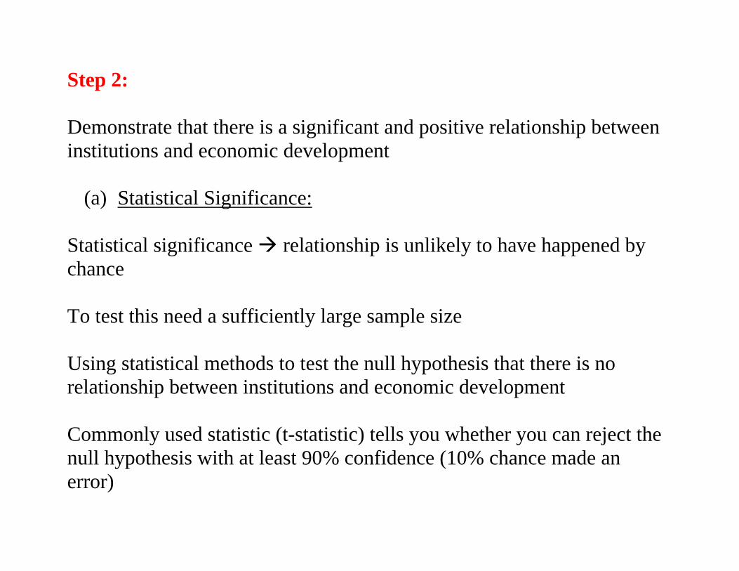
Step 2: Demonstrate that there is a significant and positive relationship between institutions and economic development

(a) Statistical Significance: Statistical significance relationship is unlikely to have happened by chance To test this need a sufficiently large sample size Using statistical methods to test the null hypothesis that there is no relationship between institutions and economic development Commonly used statistic (t-statistic) tells you whether you can reject the null hypothesis with at least 90% confidence (10% chance made an error)

(b) Other factors not driving relationship:

Could it be education driving the result? Good institutions are positively correlated with education Economic growth is positively correlated with education

If we ignore the role of education we will get a positive

relationship between economic growth and good institutions which is being driven by education (not institutions)

Need to use econometric regression techniques

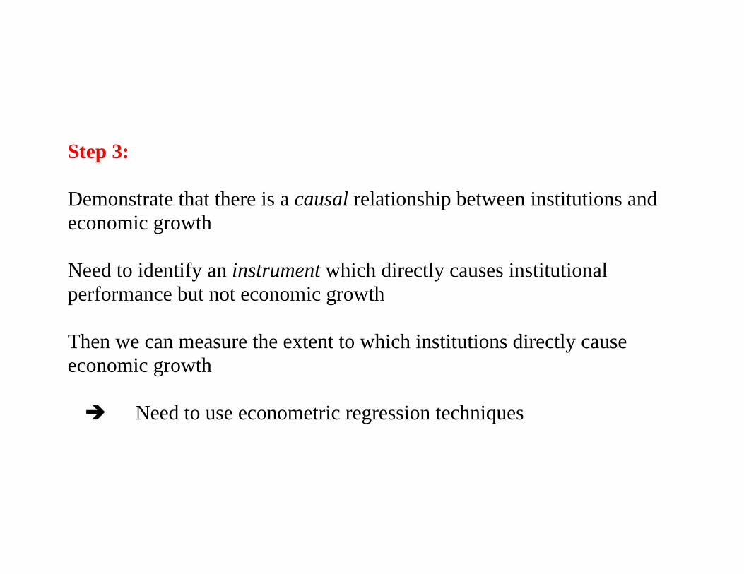
Step 3: Demonstrate that there is a causal relationship between institutions and economic growth Need to identify an instrument which directly causes institutional performance but not economic growth Then we can measure the extent to which institutions directly cause economic growth Need to use econometric regression techniques

INSTITUTIONS AND ECONOMIC DEVELOPMENT Notes from : “Colonial origins of comparative development”

(Acemoglu et. al.) What are the fundamental causes of the large differences in income per capita across countries? Differences in institutions and property rights have received attention

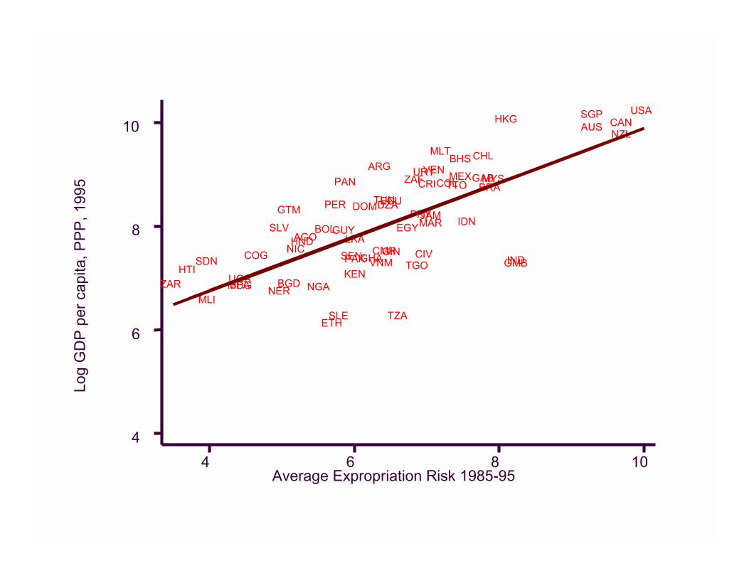
View receives support from cross-country correlations between measures of property rights and economic development

At some level -- obvious that institutions matter North and South Korea East and West Germany

One part of the country stagnated under central planning and collective ownership while the other prospered with private property and a market economy To estimate impact of institutions on economic performance we need a source of exogenous variation in institutions (an instrument)

Propose a theory of institutional differences among countries colonized by Europeans Exploit this theory to derive a possible source of exogenous variation Theory rests on three premises

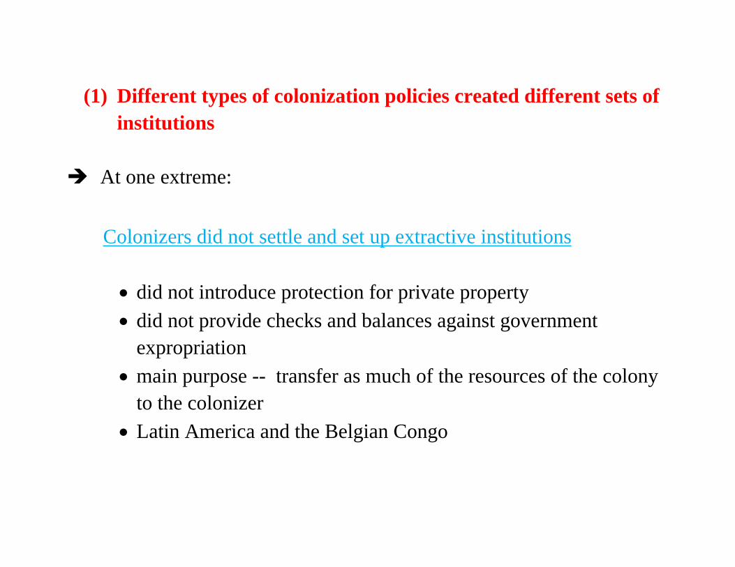
(1) Different types of colonization policies created different sets of institutions

At one extreme:

Colonizers did not settle and set up extractive institutions did not introduce protection for private property did not provide checks and balances against government

expropriation main purpose -- transfer as much of the resources of the colony

to the colonizer Latin America and the Belgian Congo

At the other extreme:

Colonizers settled and replicated European institutions strong emphasis on private property and checks against

government power

Australia, New Zealand, Canada and U.S.

(2) Colonization strategy was influenced by the feasibility of

settlements

In places where disease environment was not favorable to European settlement

formation of the extractive state was more likely

(3) The colonial state and institutions persisted even after independence.

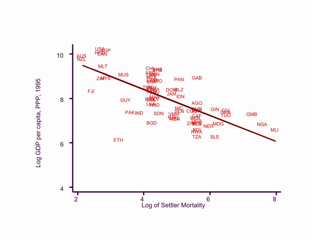
Based on these three premises: use the mortality rates of the first European settlers as an instruments

for current institutions in these countries

settler mortality settlements early institutions current institutions current economic performance

Log

GD

P pe

r cap

ita, P

PP, 1

995

Log of Settler Mortality2 4 6 8

4

6

8

10

AGO

ARG

AUS

BDI

BENBFABGD

BHS

BLZ

BOL

BRA

BRB

CAF

CAN

CHL

CIVCMRCOG

COLCRI

DOMDZAECU

EGY

ETH

FJI

GAB

GHAGINGMB

GTM

GUY

HKG

HND

HTI

IDN

IND

JAM

KENLAO

LKAMAR

MDG

MEX

MLI

MLT

MRT

MUSMYS

NER NGA

NIC

NZL

PAK

PAN

PERPRY

RWA

SDN SEN

SGP

SLE

SLV

TCD

TGO

TTOTUN

TZA

UGA

URY

USA

VEN

VNM

ZAF

ZAR

Colonies where Europeans faced higher mortality rates are today substantially poorer than colonies that were healthy for Europeans Theory implies this relationship reflects the effect of settler mortality working

through the institutions brought by Europeans

assumes there is no direct affect between settler mortality and

economic performance today

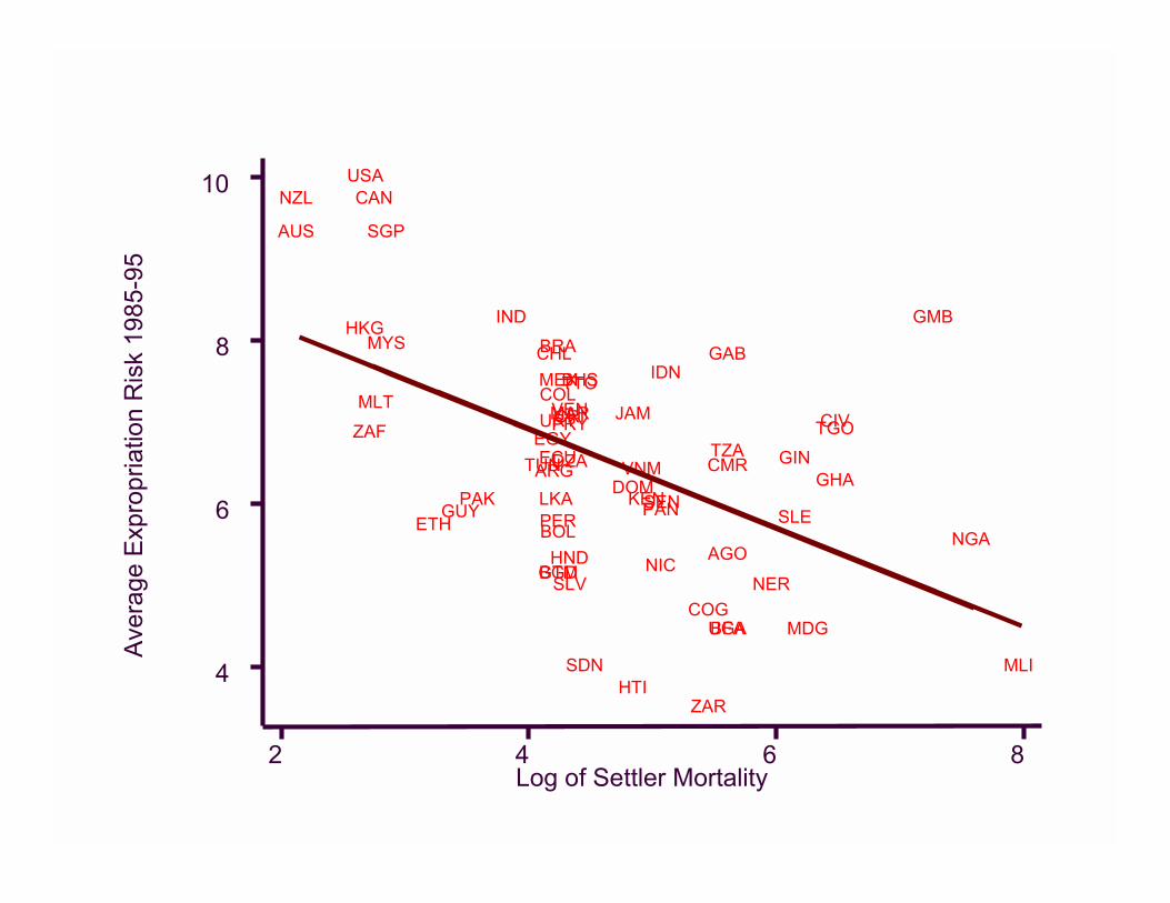
Under these assumptions: Regress current performance on current institutions and instrument the latter by settler mortality rates Focus on property rights and checks against government power use protection against risk of expropriation index as a proxy for

institutions

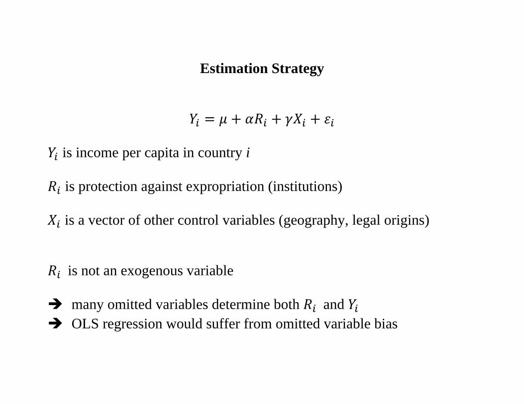
Estimation Strategy

is income per capita in country i

is protection against expropriation (institutions)

is a vector of other control variables (geography, legal origins) is not an exogenous variable

many omitted variables determine both and OLS regression would suffer from omitted variable bias

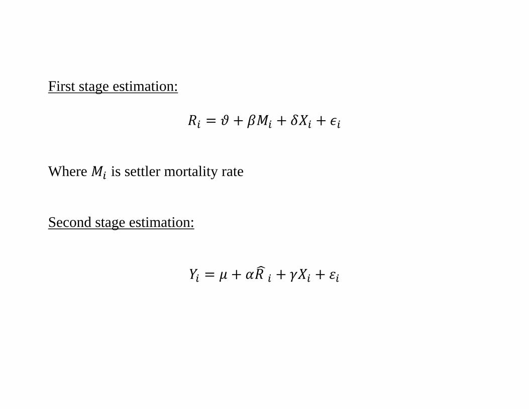
First stage estimation:

Where is settler mortality rate Second stage estimation:

Log

GD

P pe

r cap

ita, P

PP, 1

995

Average Expropriation Risk 1985-954 6 8 10

4

6

8

10

AGO

ARG

AUS

BFA BGD

BHS

BOL

BRA

CAN

CHL

CIVCMRCOG

COLCRI

DOMDZAECU

EGY

ETH

GAB

GHAGINGMB

GTM

GUY

HKG

HND

HTI

IDN

IND

JAM

KEN

LKAMAR

MDG

MEX

MLI

MLT

MYS

NER NGA

NIC

NZL

PAK

PAN

PERPRY

SDN SEN

SGP

SLE

SLV

TGO

TTOTUN

TZA

UGA

URY

USA

VEN

VNM

ZAF

ZAR

Log

GD

P pe

r cap

ita, P

PP, 1

995


4

6

8

10

AGO

ARG

AUS

BDI

BENBFABGD

BHS

BLZ

BOL

BRA

BRB

CAF

CAN

CHL

CIVCMRCOG

COLCRI

DOMDZAECU

EGY

ETH

FJI

GAB

GHAGINGMB

GTM

GUY

HKG

HND

HTI

IDN

IND

JAM

KENLAO

LKAMAR

MDG

MEX

MLI

MLT

MRT

MUSMYS

NER NGA

NIC

NZL

PAK

PAN

PERPRY

RWA

SDN SEN

SGP

SLE

SLV

TCD

TGO

TTOTUN

TZA

UGA

URY

USA

VEN

VNM

ZAF

ZAR

Aver

age

Expr

opria

tion

Ris

k 19

85-9

5


4

6

8

10

AGO

ARG

AUS

BFA

BGD

BHS

BOL

BRA

CAN

CHL

CIV

CMR

COG

COLCRI

DOMDZAECU

EGY

ETH

GAB

GHAGIN

GMB

GTM

GUY

HKG

HND

HTI

IDN

IND

JAM

KENLKA

MAR

MDG

MEX

MLI

MLT

MYS

NER

NGANIC

NZL

PAK PANPER

PRY

SDN

SEN

SGP

SLE

SLV

TGO

TTO

TUNTZA

UGA

URY

USA

VEN

VNM

ZAF

ZAR

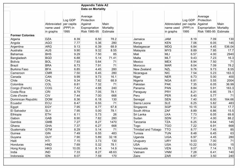
Appendix Table A2Data on Mortality

Abbreviated name used in graphs

Log GDP per capita (PPP) in 1995

Average Protection Against Expropriation Risk 1985-95

Main Mortality Estimate

Abbreviated name used in graphs

Log GDP per capita (PPP) in 1995

Average Protection Against Expropriation Risk 1985-95

Main Mortality Estimate

Former ColoniesAlgeria DZA 8.39 6.50 78.2 Jamaica JAM 8.19 7.09 130Angola AGO 7.77 5.36 280 Kenya KEN 7.06 6.05 145Argentina ARG 9.13 6.39 68.9 Madagascar MDG 6.84 4.45 536.04Australia AUS 9.90 9.32 8.55 Malaysia MYS 8.89 7.95 17.7Bahamas BHS 9.29 7.50 85 Mali MLI 6.57 4.00 2940Bangladesh BGD 6.88 5.14 71.41 Malta MLT 9.43 7.23 16.3Bolivia BOL 7.93 5.64 71 Mexico MEX 8.94 7.50 71Brazil BRA 8.73 7.91 71 Morocco MAR 8.04 7.09 78.2Burkina Faso BFA 6.85 4.45 280 New Zealand NZL 9.76 9.73 8.55Cameroon CMR 7.50 6.45 280 Nicaragua NIC 7.54 5.23 163.3Canada CAN 9.99 9.73 16.1 Niger NER 6.73 5.00 400Chile CHL 9.34 7.82 68.9 Nigeria NGA 6.81 5.55 2004Colombia COL 8.81 7.32 71 Pakistan PAK 7.35 6.05 36.99Congo (French) COG 7.42 4.68 240 Panama PAN 8.84 5.91 163.3Costa Rica CRI 8.79 7.05 78.1 Paraguay PRY 8.21 6.95 78.1Cote d'Ivoire CIV 7.44 7.00 668 Peru PER 8.40 5.77 71Dominican Republic DOM 8.36 6.18 130 Senegal SEN 7.40 6.00 164.66Ecuador ECU 8.47 6.55 71 Sierra Leone SLE 6.25 5.82 483Egypt EGY 7.95 6.77 67.8 Singapore SGP 10.15 9.32 17.7El Salvador SLV 7.95 5.00 78.1 South Africa ZAF 8.89 6.86 15.5Ethiopia ETH 6.11 5.73 26 Sri Lanka LKA 7.73 6.05 69.8Gabon GAB 8.90 7.82 280 Sudan SDN 7.31 4.00 88.2Gambia GMB 7.27 8.27 1470 Tanzania TZA 6.25 6.64 145Ghana GHA 7.37 6.27 668 Togo TGO 7.22 6.91 668Guatemala GTM 8.29 5.14 71 Trinidad and Tobago TTO 8.77 7.45 85Guinea GIN 7.49 6.55 483 Tunisia TUN 8.48 6.45 63Guyana GUY 7.90 5.89 32.18 Uganda UGA 6.97 4.45 280Haiti HTI 7.15 3.73 130 Uruguary URY 9.03 7.00 71Honduras HND 7.69 5.32 78.1 USA USA 10.22 10.00 15Hong Kong HKG 10.05 8.14 14.9 Venezuela VEN 9.07 7.14 78.1India IND 7.33 8.27 48.63 Vietnam VNM 7.28 6.41 140Indonesia IDN 8.07 7.59 170 Zaire ZAR 6.87 3.50 240

Table 4IV Regressions of log GDP per capita

Base Sample

Base Sample

Base Sample without

neo-Europes

Base Sample without

neo-Europes

Base Sample without Africa

Base Sample without Africa

Base Sample

with Continent Dummies

Base Sample

with Continent Dummies

Base Sample, dep. var. is log

output per worker (1) (2) (3) (4) (5) (6) (7) (8) (9)

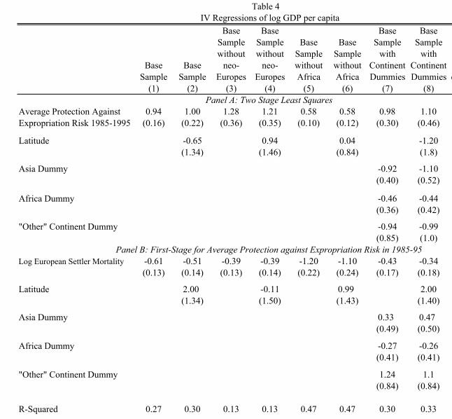
Panel A: Two Stage Least SquaresAverage Protection Against 0.94 1.00 1.28 1.21 0.58 0.58 0.98 1.10 0.98Expropriation Risk 1985-1995 (0.16) (0.22) (0.36) (0.35) (0.10) (0.12) (0.30) (0.46) (0.17)

Latitude -0.65 0.94 0.04 -1.20(1.34) (1.46) (0.84) (1.8)

Asia Dummy -0.92 -1.10(0.40) (0.52)

Africa Dummy -0.46 -0.44(0.36) (0.42)

"Other" Continent Dummy -0.94 -0.99(0.85) (1.0)

Panel B: First-Stage for Average Protection against Expropriation Risk in 1985-95Log European Settler Mortality -0.61 -0.51 -0.39 -0.39 -1.20 -1.10 -0.43 -0.34 -0.63

(0.13) (0.14) (0.13) (0.14) (0.22) (0.24) (0.17) (0.18) (0.13)

Latitude 2.00 -0.11 0.99 2.00(1.34) (1.50) (1.43) (1.40)

Asia Dummy 0.33 0.47(0.49) (0.50)

Africa Dummy -0.27 -0.26(0.41) (0.41)

"Other" Continent Dummy 1.24 1.1(0.84) (0.84)

R-Squared 0.27 0.30 0.13 0.13 0.47 0.47 0.30 0.33 0.28

Panel C: Ordinary Least SquaresAverage Protection Against 0.52 0.47 0.49 0.47 0.48 0.47 0.42 0.40 0.46Expropriation Risk 1985-1995 (0.06) (0.06) (0.08) (0.07) (0.07) (0.07) (0.06) (0.06) (0.06)

Number of Observations 64 64 60 60 37 37 64 64 61

The dependent variable in columns 1-8 is log GDP per capita in 1995, PPP basis. The dependent variable in column 9 is log output per worker, from Hall and Jones (1999). "Average Protection Against Expropriation Risk 1985-95" is measured on a scale from 0 to 10, where a higher score means more protection against risk of expropriation of investment by the government, from Political Risk Services. Panel A reports the two stage least squares estimates, instrumenting for protection against expropriation risk using log settler mortality; Panel B reports the corresponding first stage. Panel C reports the coefficient from an OLS regression of the dependent variable against average protection against expropriation risk. Standard errors are in parentheses. In regressions with continent dummies, the dummy for America is omitted. See Appendix Table A1 for more detailed variable descriptions and sources.

Regressions in Table 4 control for: Latitude (geography) Continent dummies

What other variables could be driving the result?

Table 5 Control for legal origins

Control for identity of colonizer

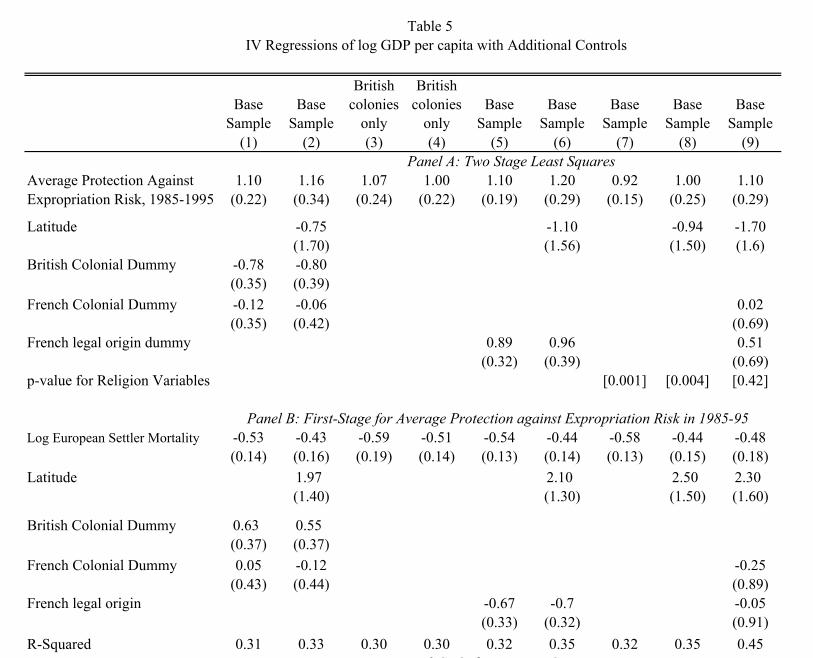
Table 5IV Regressions of log GDP per capita with Additional Controls

Base Sample

Base Sample

British colonies

only

British colonies

onlyBase

SampleBase

SampleBase

SampleBase

SampleBase

Sample(1) (2) (3) (4) (5) (6) (7) (8) (9)

Panel A: Two Stage Least SquaresAverage Protection Against 1.10 1.16 1.07 1.00 1.10 1.20 0.92 1.00 1.10Expropriation Risk, 1985-1995 (0.22) (0.34) (0.24) (0.22) (0.19) (0.29) (0.15) (0.25) (0.29)

Latitude -0.75 -1.10 -0.94 -1.70(1.70) (1.56) (1.50) (1.6)

British Colonial Dummy -0.78 -0.80(0.35) (0.39)

French Colonial Dummy -0.12 -0.06 0.02(0.35) (0.42) (0.69)

French legal origin dummy 0.89 0.96 0.51(0.32) (0.39) (0.69)

p-value for Religion Variables [0.001] [0.004] [0.42]


(0.14) (0.16) (0.19) (0.14) (0.13) (0.14) (0.13) (0.15) (0.18)Latitude 1.97 2.10 2.50 2.30

(1.40) (1.30) (1.50) (1.60)

British Colonial Dummy 0.63 0.55(0.37) (0.37)

French Colonial Dummy 0.05 -0.12 -0.25(0.43) (0.44) (0.89)

French legal origin -0.67 -0.7 -0.05(0.33) (0.32) (0.91)

R-Squared 0.31 0.33 0.30 0.30 0.32 0.35 0.32 0.35 0.45Panel C: Ordinary Least Squares

Average Protection Against 0.53 0.47 0.61 0.47 0.56 0.56 0.53 0.47 0.47Expropriation Risk, 1985-1995 (0.19) (0.07) (0.09) (0.06) (0.06) (0.06) (0.06) (0.06) (0.06)

Number of Observations 64 64 25 25 64 64 64 64 64

Panel A reports the two stage least squares estimates with log GDP per capita (PPP basis) in 1995 as dependent variable, and Panel B reports the corresponding first stage. The base case in columns 1 and 2 is all colonies that were neither French nor British. The religion variables are included in the first stage of columns 7 and 8 but not reported here (to save space). Panel C reports the OLS coefficient from regressing log GDP per capita on average protection against expropriation risk, with the other control variables indicated in that column (full results not reported to save space). Standard errors are in parentheses. The religion variables are percentage of population that are Catholics, Muslims, and "other" religions; Protestant is the base case. Our sample is all either French or British legal origin (as defined by La Porta et al 1999.)

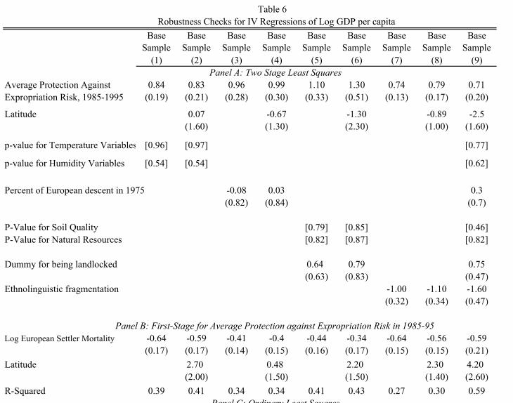
Table 6: Control for climate variables

Control for natural resources

Control for land characteristics

Control for percent of current population which is of European

descent

Table 6Robustness Checks for IV Regressions of Log GDP per capita

Base Sample

Base Sample

Base Sample

Base Sample

Base Sample

Base Sample

Base Sample

Base Sample

Base Sample

(1) (2) (3) (4) (5) (6) (7) (8) (9)Panel A: Two Stage Least Squares

Average Protection Against 0.84 0.83 0.96 0.99 1.10 1.30 0.74 0.79 0.71Expropriation Risk, 1985-1995 (0.19) (0.21) (0.28) (0.30) (0.33) (0.51) (0.13) (0.17) (0.20)

Latitude 0.07 -0.67 -1.30 -0.89 -2.5(1.60) (1.30) (2.30) (1.00) (1.60)

p-value for Temperature Variables [0.96] [0.97] [0.77]

p-value for Humidity Variables [0.54] [0.54] [0.62]

Percent of European descent in 1975 -0.08 0.03 0.3(0.82) (0.84) (0.7)

P-Value for Soil Quality [0.79] [0.85] [0.46]P-Value for Natural Resources [0.82] [0.87] [0.82]

Dummy for being landlocked 0.64 0.79 0.75(0.63) (0.83) (0.47)

Ethnolinguistic fragmentation -1.00 -1.10 -1.60(0.32) (0.34) (0.47)


(0.17) (0.17) (0.14) (0.15) (0.16) (0.17) (0.15) (0.15) (0.21)Latitude 2.70 0.48 2.20 2.30 4.20

(2.00) (1.50) (1.50) (1.40) (2.60)R-Squared 0.39 0.41 0.34 0.34 0.41 0.43 0.27 0.30 0.59

Panel C: Ordinary Least SquaresAverage Protection Against 0.41 0.38 0.39 0.38 0.46 0.42 0.46 0.45 0.38Expropriation Risk, 1985-1995 (0.06) (0.06) (0.06) (0.06) (0.07) (0.07) (0.05) (0.06) (0.06)

Panel A reports the two stage least squares estimates with log GDP per capita (PPP basis) in 1995, and Panel B reports the corresponding first stages. Panel C reports the OLS coefficient from regressing log GDP per capita on average protection against expropriation risk, with the other control variables indicated in that column (full results not reported to save space). Standard errors are in parentheses. All regressions have 64 observations, except those including natural resources, which have 63 observations. The temperature and humidity variables are: average, minimum and maximum monthly high temperatures, and minimum and maximum monthly low temperatures, and morning minimum and maximum humidity, and afternoon minimum and maximum humidity. In the table we report joint significance levels for these variables (from Philip Parker, 1997). Measures of natural resources are: percent of world gold reserves today, percent of world iron reserves today, percent of world zinc reserves today, number of minerals present in country, and oil resources (thousands of barrels per capita.) Measures of soil quality/climate are steppe (low latitude), desert (low latitude), steppe (middle latitude), desert (middle latitude), dry steppe wasteland, desert dry winter, and highland. See Appendix Table A1 for more detailed variable definitions and sources.

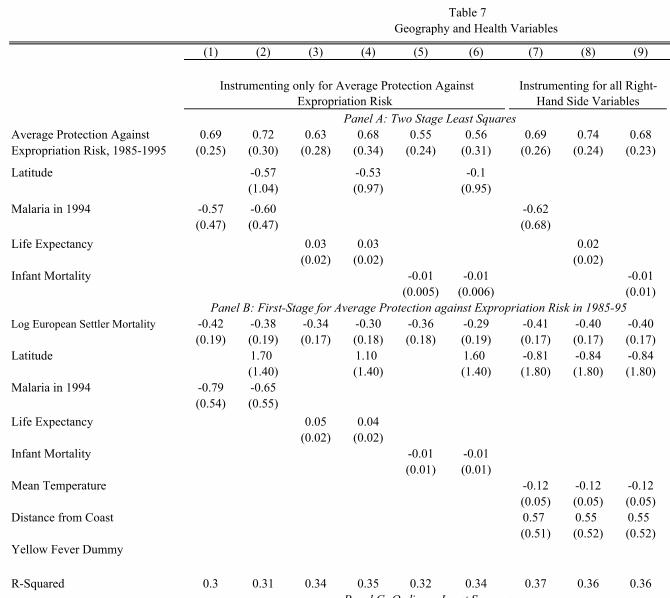
Table 7: Control for disease environment Control for health indicators

Table 7Geography and Health Variables

(1) (2) (3) (4) (5) (6) (7) (8) (9) (10) (11)

Panel A: Two Stage Least SquaresAverage Protection Against 0.69 0.72 0.63 0.68 0.55 0.56 0.69 0.74 0.68 0.91 0.90Expropriation Risk, 1985-1995 (0.25) (0.30) (0.28) (0.34) (0.24) (0.31) (0.26) (0.24) (0.23) (0.24) (0.32)

Latitude -0.57 -0.53 -0.1(1.04) (0.97) (0.95)

Malaria in 1994 -0.57 -0.60 -0.62(0.47) (0.47) (0.68)

Life Expectancy 0.03 0.03 0.02(0.02) (0.02) (0.02)

Infant Mortality -0.01 -0.01 -0.01(0.005) (0.006) (0.01)


(0.19) (0.19) (0.17) (0.18) (0.18) (0.19) (0.17) (0.17) (0.17)Latitude 1.70 1.10 1.60 -0.81 -0.84 -0.84

(1.40) (1.40) (1.40) (1.80) (1.80) (1.80)Malaria in 1994 -0.79 -0.65

(0.54) (0.55)Life Expectancy 0.05 0.04

(0.02) (0.02)Infant Mortality -0.01 -0.01

(0.01) (0.01)Mean Temperature -0.12 -0.12 -0.12

(0.05) (0.05) (0.05)Distance from Coast 0.57 0.55 0.55

(0.51) (0.52) (0.52)Yellow Fever Dummy -1.10 -0.81

(0.41) (0.38)R-Squared 0.3 0.31 0.34 0.35 0.32 0.34 0.37 0.36 0.36 0.10 0.32

Panel C: Ordinary Least SquaresAverage Protection Against 0.35 0.35 0.28 0.28 0.29 0.28 0.35 0.29 0.29 0.48 0.39Expropriation Risk, 1985-1995 (0.06) (0.06) (0.05) (0.05) (0.05) (0.05) (0.06) (0.05) (0.05) (0.06) (0.06)

Number of Observations 62 62 60 60 60 60 60 59 59 64 64

Panel A reports the two stage least squares estimates with log GDP per capita (PPP basis) in 1995, and Panel B reports the corresponding first stages. Panel C reports the coefficient from an OLS regression with log GDP per capita as the dependent variable and average protection against expropriation risk and the other control variables indicated in each column as independent variables (full results not reported to save space). Standard errors are in parentheses. Columns 1-6 instrument for average protection against expropriation risk using log mortality and assume that the other regressors are exogenous. Columns 7, 8 and 9 include as instruments average temperature, amount of territory within 100 km of the coast, and latitude (from McArthur and Sachs 2001.) Columns 10 and 11 use a dummy variable for whether or not a country was subject to yellow fever epidemics before 1900 as an instrument for average protection against expropriation. See Appendix Table A1 for more detailed variable definitions and sources.

Instrumenting only for Average Protection Against Expropriation Risk

Instrumenting for all Right-Hand Side Variables

Instrument only Average Protect.

Against Exprop. Risk

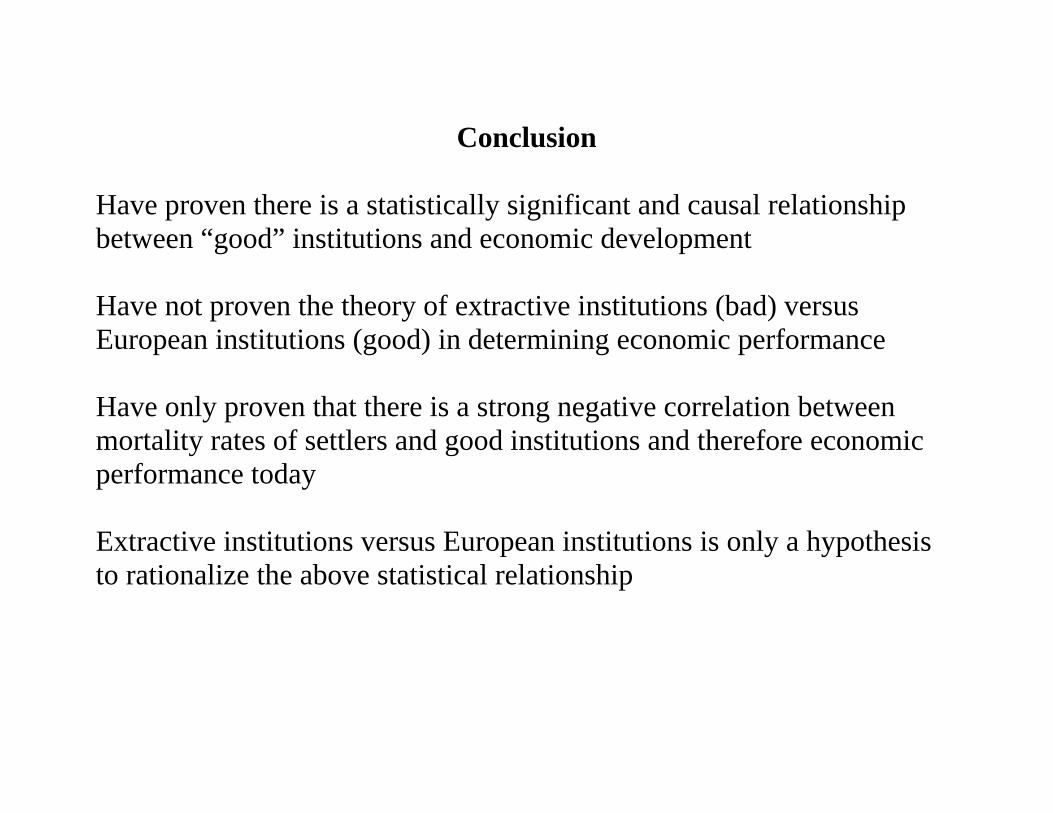
Conclusion

Have proven there is a statistically significant and causal relationship between “good” institutions and economic development Have not proven the theory of extractive institutions (bad) versus European institutions (good) in determining economic performance Have only proven that there is a strong negative correlation between mortality rates of settlers and good institutions and therefore economic performance today Extractive institutions versus European institutions is only a hypothesis to rationalize the above statistical relationship

Notes from “The long-term effects of Africa’s slave trade” (Nunn) Africa’s economic performance in second half of the 20th century has been very poor One explanation for Africa’s underdevelopment is its history of extraction characterized by two events: slave trades colonialism

Earlier work (Acemoglu et. al.) focus on countries’ colonial experience and current economic development Reasons to expect that slave trades may have been at least as important as colonial rule for Africa’s development For period of nearly 500 years (1400-1900) African continent simultaneously experienced four slave trades By comparison colonial rule lasted from 1885 to 1960 (only 75 years)

Empirical examination

Examine importance of Africa’s slave trades in shaping Africa’s current economic development Construct measures of: number of slaves from each country in Africa in each century between 1400 and 1900

Estimates are constructed by combining: data from ship records on the number of slaves shipped from each

African port or region data from a variety of historical documents that report the ethnic

identities of slaves that were shipped from Africa

Find robust negative relationship between the number of slaves exported from each country and subsequent economic performance The African countries that are the poorest today are the ones from which most slaves were taken This finding cannot be taken as conclusive evidence that the slave trades caused differences in subsequent economic development An alternative explanation is that countries that were initially the most economically and socially underdeveloped selected into the slave trades and these countries continue to be the most underdeveloped today Need to identify the direction of causality (find an instrumental

variable)

Historical Background

Between 1400 and 1900 -- African continent experienced four simultaneous slave trades Largest and most well known is the trans-Atlantic slave trade beginning in the 15th century slaves shipped from West Central Africa and Eastern Africa to

European colonies in the New World

Three other slave trades: Trans-Saharan Red Sea Indian Ocean

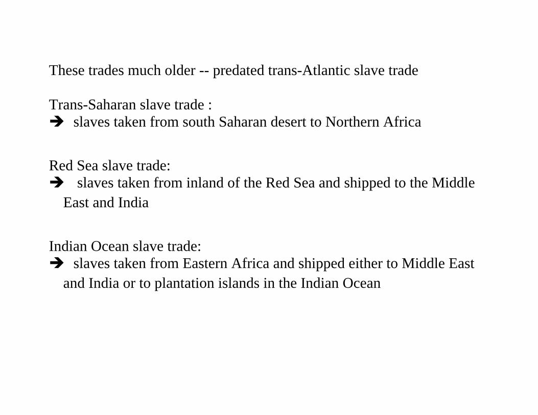
These trades much older -- predated trans-Atlantic slave trade Trans-Saharan slave trade : slaves taken from south Saharan desert to Northern Africa

Red Sea slave trade: slaves taken from inland of the Red Sea and shipped to the Middle

East and India

Indian Ocean slave trade: slaves taken from Eastern Africa and shipped either to Middle East

and India or to plantation islands in the Indian Ocean

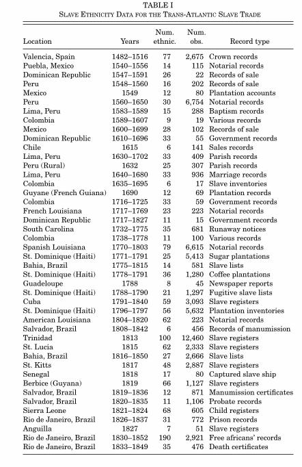
THE LONG-TERM EFFECTS OF AFRICA’S SLAVE TRADES 147

TABLE ISLAVE ETHNICITY DATA FOR THE TRANS-ATLANTIC SLAVE TRADE

Num. Num.Location Years ethnic. obs. Record type

Valencia, Spain 1482–1516 77 2,675 Crown recordsPuebla, Mexico 1540–1556 14 115 Notarial recordsDominican Republic 1547–1591 26 22 Records of salePeru 1548–1560 16 202 Records of saleMexico 1549 12 80 Plantation accountsPeru 1560–1650 30 6,754 Notarial recordsLima, Peru 1583–1589 15 288 Baptism recordsColombia 1589–1607 9 19 Various recordsMexico 1600–1699 28 102 Records of saleDominican Republic 1610–1696 33 55 Government recordsChile 1615 6 141 Sales recordsLima, Peru 1630–1702 33 409 Parish recordsPeru (Rural) 1632 25 307 Parish recordsLima, Peru 1640–1680 33 936 Marriage recordsColombia 1635–1695 6 17 Slave inventoriesGuyane (French Guiana) 1690 12 69 Plantation recordsColombia 1716–1725 33 59 Government recordsFrench Louisiana 1717–1769 23 223 Notarial recordsDominican Republic 1717–1827 11 15 Government recordsSouth Carolina 1732–1775 35 681 Runaway noticesColombia 1738–1778 11 100 Various recordsSpanish Louisiana 1770–1803 79 6,615 Notarial recordsSt. Dominique (Haiti) 1771–1791 25 5,413 Sugar plantationsBahia, Brazil 1775–1815 14 581 Slave listsSt. Dominique (Haiti) 1778–1791 36 1,280 Coffee plantationsGuadeloupe 1788 8 45 Newspaper reportsSt. Dominique (Haiti) 1788–1790 21 1,297 Fugitive slave listsCuba 1791–1840 59 3,093 Slave registersSt. Dominique (Haiti) 1796–1797 56 5,632 Plantation inventoriesAmerican Louisiana 1804–1820 62 223 Notarial recordsSalvador, Brazil 1808–1842 6 456 Records of manumissionTrinidad 1813 100 12,460 Slave registersSt. Lucia 1815 62 2,333 Slave registersBahia, Brazil 1816–1850 27 2,666 Slave listsSt. Kitts 1817 48 2,887 Slave registersSenegal 1818 17 80 Captured slave shipBerbice (Guyana) 1819 66 1,127 Slave registersSalvador, Brazil 1819–1836 12 871 Manumission certificatesSalvador, Brazil 1820–1835 11 1,106 Probate recordsSierra Leone 1821–1824 68 605 Child registersRio de Janeiro, Brazil 1826–1837 31 772 Prison recordsAnguilla 1827 7 51 Slave registersRio de Janeiro, Brazil 1830–1852 190 2,921 Free africans’ recordsRio de Janeiro, Brazil 1833–1849 35 476 Death certificates

152 QUARTERLY JOURNAL OF ECONOMICS

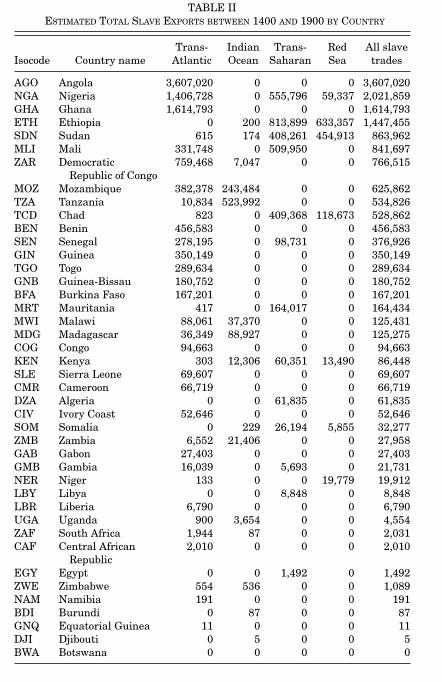
TABLE IIESTIMATED TOTAL SLAVE EXPORTS BETWEEN 1400 AND 1900 BY COUNTRY

Trans- Indian Trans- Red All slaveIsocode Country name Atlantic Ocean Saharan Sea trades

AGO Angola 3,607,020 0 0 0 3,607,020NGA Nigeria 1,406,728 0 555,796 59,337 2,021,859GHA Ghana 1,614,793 0 0 0 1,614,793ETH Ethiopia 0 200 813,899 633,357 1,447,455SDN Sudan 615 174 408,261 454,913 863,962MLI Mali 331,748 0 509,950 0 841,697ZAR Democratic 759,468 7,047 0 0 766,515

Republic of CongoMOZ Mozambique 382,378 243,484 0 0 625,862TZA Tanzania 10,834 523,992 0 0 534,826TCD Chad 823 0 409,368 118,673 528,862BEN Benin 456,583 0 0 0 456,583SEN Senegal 278,195 0 98,731 0 376,926GIN Guinea 350,149 0 0 0 350,149TGO Togo 289,634 0 0 0 289,634GNB Guinea-Bissau 180,752 0 0 0 180,752BFA Burkina Faso 167,201 0 0 0 167,201MRT Mauritania 417 0 164,017 0 164,434MWI Malawi 88,061 37,370 0 0 125,431MDG Madagascar 36,349 88,927 0 0 125,275COG Congo 94,663 0 0 0 94,663KEN Kenya 303 12,306 60,351 13,490 86,448SLE Sierra Leone 69,607 0 0 0 69,607CMR Cameroon 66,719 0 0 0 66,719DZA Algeria 0 0 61,835 0 61,835CIV Ivory Coast 52,646 0 0 0 52,646SOM Somalia 0 229 26,194 5,855 32,277ZMB Zambia 6,552 21,406 0 0 27,958GAB Gabon 27,403 0 0 0 27,403GMB Gambia 16,039 0 5,693 0 21,731NER Niger 133 0 0 19,779 19,912LBY Libya 0 0 8,848 0 8,848LBR Liberia 6,790 0 0 0 6,790UGA Uganda 900 3,654 0 0 4,554ZAF South Africa 1,944 87 0 0 2,031CAF Central African 2,010 0 0 0 2,010

RepublicEGY Egypt 0 0 1,492 0 1,492ZWE Zimbabwe 554 536 0 0 1,089NAM Namibia 191 0 0 0 191BDI Burundi 0 87 0 0 87GNQ Equatorial Guinea 11 0 0 0 11DJI Djibouti 0 5 0 0 5BWA Botswana 0 0 0 0 0


TABLE II(CONTINUED)

Trans- Indian Trans- Red All slaveIsocode Country name Atlantic Ocean Saharan Sea trades

CPV Cape Verde Islands 0 0 0 0 0COM Comoros 0 0 0 0 0LSO Lesotho 0 0 0 0 0MUS Mauritius 0 0 0 0 0MAR Morocco 0 0 0 0 0RWA Rwanda 0 0 0 0 0STP Sao Tome & Principe 0 0 0 0 0SWZ Swaziland 0 0 0 0 0SYC Seychelles 0 0 0 0 0TUN Tunisia 0 0 0 0 0

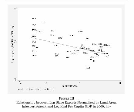
FIGURE IIIRelationship between Log Slave Exports Normalized by Land Area,

ln(exports/area), and Log Real Per Capita GDP in 2000, ln y

between 1400 and 1900 normalized by land area and the naturallog of per capita GDP in 2000.7 As shown in the figure, a negative

7. Because the natural log of zero is undefined, I take the natural log of 0.1. AsI show in the Appendix, the results are robust to the omission of these zero-exportcountries.

Estimation Equation

is per capita GDP in country i

is vector of variables reflecting origin of colonizer prior to independence

is vector of variables reflecting geography and climate


TABLE IIIRELATIONSHIP BETWEEN SLAVE EXPORTS AND INCOME

Dependent variable is log real per capita GDP in 2000, ln y

(1) (2) (3) (4) (5) (6)

ln(exports/area) −0.112∗∗∗ −0.076∗∗∗ −0.108∗∗∗ −0.085∗∗ −0.103∗∗∗ −0.128∗∗∗(0.024) (0.029) (0.037) (0.035) (0.034) (0.034)

Distance from 0.016 −0.005 0.019 0.023 0.006equator (0.017) (0.020) (0.018) (0.017) (0.017)

Longitude 0.001 −0.007 −0.004 −0.004 −0.009(0.005) (0.006) (0.006) (0.005) (0.006)

Lowest monthly −0.001 0.008 0.0001 −0.001 −0.002rainfall (0.007) (0.008) (0.007) (0.006) (0.008)

Avg max humidity 0.009 0.008 0.009 0.015 0.013(0.012) (0.012) (0.012) (0.011) (0.010)

Avg min −0.019 −0.039 −0.005 −0.015 −0.037temperature (0.028) (0.028) (0.027) (0.026) (0.025)

ln(coastline/area) 0.085∗∗ 0.092∗∗ 0.095∗∗ 0.082∗∗ 0.083∗∗(0.039) (0.042) (0.042) (0.040) (0.037)

Island indicator −0.398 −0.150(0.529) (0.516)

Percent Islamic −0.008∗∗∗ −0.006∗ −0.003(0.003) (0.003) (0.003)

French legal origin 0.755 0.643 −0.141(0.503) (0.470) (0.734)

North Africa 0.382 −0.304indicator (0.484) (0.517)

ln(gold prod/pop) 0.011 0.014(0.017) (0.015)

ln(oil prod/pop) 0.078∗∗∗ 0.088∗∗∗(0.027) (0.025)

ln(diamond −0.039 −0.048prod/pop) (0.043) (0.041)

Colonizer fixed Yes Yes Yes Yes Yes Yeseffects

Number obs. 52 52 42 52 52 42R2 .51 .60 .63 .71 .77 .80

Notes. OLS estimates of (1) are reported. The dependent variable is the natural log of real per capitaGDP in 2000, ln y. The slave export variable ln(exports/area) is the natural log of the total number of slavesexported from each country between 1400 and 1900 in the four slave trades normalized by land area. Thecolonizer fixed effects are indicator variables for the identity of the colonizer at the time of independence.Coefficients are reported with standard errors in brackets. ∗∗∗ , ∗∗ , and ∗ indicate significance at the 1%, 5%,and 10% levels.

for slave exports remains negative and significant, and the mag-nitude of the estimated coefficient actually increases.9

9. One may also be concerned that the inclusion of the countries in southernAfrica—namely South Africa, Swaziland, and Lesotho—may also be biasing theresults. As I report in the Appendix, the results are robust to also omitting this

Direction of causality OLS estimates show there is a relationship between slave exports and current economic performance Still unclear whether slave trades have a causal impact on current income Alternative explanation for relationship: societies that were initially under developed selected into slave

trades these societies continue to be under developed today

Therefore we observe a negative relationship between slave exports and current income even though the slave trades did not have any effect on subsequent economic development

Two strategies to evaluate whether there is a causal effect of the slave trades on income

(1) Using historic data: can evaluate importance and characteristics of selection into the slave trades

(2) Find instruments for slave exports

Historical Evidence on Selection during the Slave Trades Using data on initial population densities Check whether more or less prosperous areas selected into the slave

trades

Population density is a reasonable indicator of economic prosperity


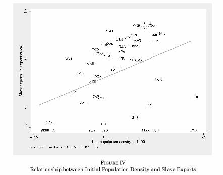
FIGURE IVRelationship between Initial Population Density and Slave Exports

obtained if civil wars or conflicts could be instigated (Barry 1992;Inikori 2003). As well, societies that were the most violent andhostile, and therefore the least developed, were often best ableto resist European efforts to purchase slaves. For example, theslave trade in Gabon was limited because of the defiance andviolence of its inhabitants toward the Portuguese. This resistancecontinued for centuries, and as a result the Portuguese were forcedto concentrate their efforts along the coast further south (Hall2005, pp. 60–64).

Using data on initial population densities, I check whether itwas the more prosperous or less prosperous areas that selectedinto the slave trades. Acemoglu, Johnson, and Robinson (2002)have shown that population density is a reasonable indicator ofeconomic prosperity. Figure IV shows the relationship betweenthe natural log of population density in 1400 and ln(exports/area).The data confirm the historical evidence on selection during theslave trades.12 The figure shows that the parts of Africa that were

12. The relationship is similar if one excludes island and North African coun-tries, or if one normalizes slave exports by population rather than land area.

Figure shows that parts of Africa that were the most prosperous in 1400 (measured by population density) tend also to be the areas that were most impacted by the slave trades evidence suggests that societies that were the most prosperous, not

the most under developed, that selected into the slave trades

unlikely that the strong relationship between slave exports and

current income is driven by selection

Instrumental Variables

Use instruments that are correlated with slave exports but are uncorrelated with other country characteristics As instruments for slave exports use distances from each African country to the locations where the

slaves were demanded

Validity of these instruments relies on presumption: although location of demand influenced the location of supply location of supply did not influence location of demand

If sugar plantations were established in West Indies because West Indies were close to Western Coast of Africa instruments not valid

If instead slaves were taken from Western Africa, because it was relatively close to plantation economies in West Indies instruments are valid

Historical evidence suggests this to be true location for demand of African slaves was determined by a number

of factors all unrelated to the supply of slaves

In West Indies and southern U.S. slaves were imported because of climates suitable for growing commodities such as sugar and tobacco Existence of gold and silver mines was determinant for demand of slaves in Brazil In northern Sahara, Arabia, and Persia slaves were needed to work in salt mines In the Red Sea area slaves were used as pearl divers


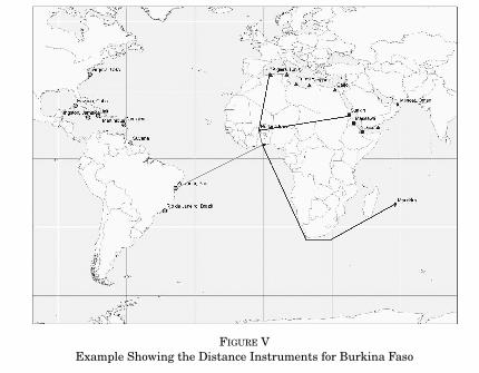
FIGURE VExample Showing the Distance Instruments for Burkina Faso

4. The overland distance from a country’s centroid to the clos-est port of export for the Red Sea slave trade. The portsare Massawa, Suakin, and Djibouti.14

The instruments are illustrated in Figure V, which shows thefour distances for Burkina Faso. The ports in each of the fourslave trades are represented by different colored symbols, and theshortest distances by colored lines. Details of the construction ofthe instruments are given in the Appendix.15

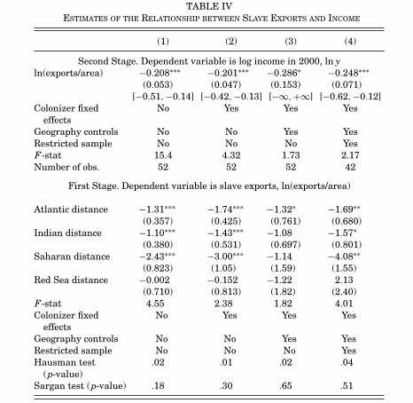
The IV estimates are reported in Table IV. The first columnreports estimates without control variables, the second columnincludes colonizer fixed effects, and the third and fourth columnsinclude colonizer fixed effects and geography controls. In column(4), the sample excludes islands and North African countries.

14. For island countries, one cannot reach the ports of the Saharan or RedSea slave trades by traveling overland. For these countries I use the sum of thesailing distance and overland distance.

15. An alternative strategy is to also include the distance from the centroidto the coast (which is also shown in Figure V) as an additional instrument, sincethis distance is part of the total distance to the markets in the Indian Ocean andtrans-Atlantic slave trades. The results are essentially identical if this distance isalso included as an additional instrument.


TABLE IVESTIMATES OF THE RELATIONSHIP BETWEEN SLAVE EXPORTS AND INCOME

(1) (2) (3) (4)

Second Stage. Dependent variable is log income in 2000, ln yln(exports/area) −0.208∗∗∗ −0.201∗∗∗ −0.286∗ −0.248∗∗∗

(0.053) (0.047) (0.153) (0.071)[−0.51, −0.14] [−0.42, −0.13] [−∞, +∞] [−0.62, −0.12]

Colonizer fixed No Yes Yes Yeseffects

Geography controls No No Yes YesRestricted sample No No No YesF-stat 15.4 4.32 1.73 2.17Number of obs. 52 52 52 42

First Stage. Dependent variable is slave exports, ln(exports/area)

Atlantic distance −1.31∗∗∗ −1.74∗∗∗ −1.32∗ −1.69∗∗(0.357) (0.425) (0.761) (0.680)

Indian distance −1.10∗∗∗ −1.43∗∗∗ −1.08 −1.57∗(0.380) (0.531) (0.697) (0.801)

Saharan distance −2.43∗∗∗ −3.00∗∗∗ −1.14 −4.08∗∗(0.823) (1.05) (1.59) (1.55)

Red Sea distance −0.002 −0.152 −1.22 2.13(0.710) (0.813) (1.82) (2.40)

F-stat 4.55 2.38 1.82 4.01Colonizer fixed No Yes Yes Yes

effectsGeography controls No No Yes YesRestricted sample No No No YesHausman test .02 .01 .02 .04

(p-value)Sargan test (p-value) .18 .30 .65 .51

Notes. IV estimates of (1) are reported. Slave exports ln(exports/area) is the natural log of the total numberof slaves exported from each country between 1400 and 1900 in the four slave trades normalized by land area.The colonizer fixed effects are indicator variables for the identity of the colonizer at the time of independence.Coefficients are reported, with standard errors in brackets. For the endogenous variable ln(exports/area), Ialso report 95% confidence regions based on Moreira’s (2003) conditional likelihood ratio (CLR) approach.These are reported in square brackets. The p-value of the Hausman test is for the Wu–Hausman chi-squaredtest. ∗∗∗ , ∗∗ , and ∗ indicate significance at the 1%, 5%, and 10% levels. The “restricted sample” excludes islandand North African countries. The “geography controls” are distance from equator, longitude, lowest monthlyrainfall, avg max humidity, avg min temperature, and ln(coastline/area).

The first-stage estimates are reported in the bottom panel ofthe table. The coefficients for the instruments are generally neg-ative, suggesting that the further a country was from slave mar-kets, the fewer slaves it exported.16 The exception is the distance

16. The specifications assume a linear first-stage relationship. The estimatesare similar if one also allows for a nonlinear relationship between slave exports

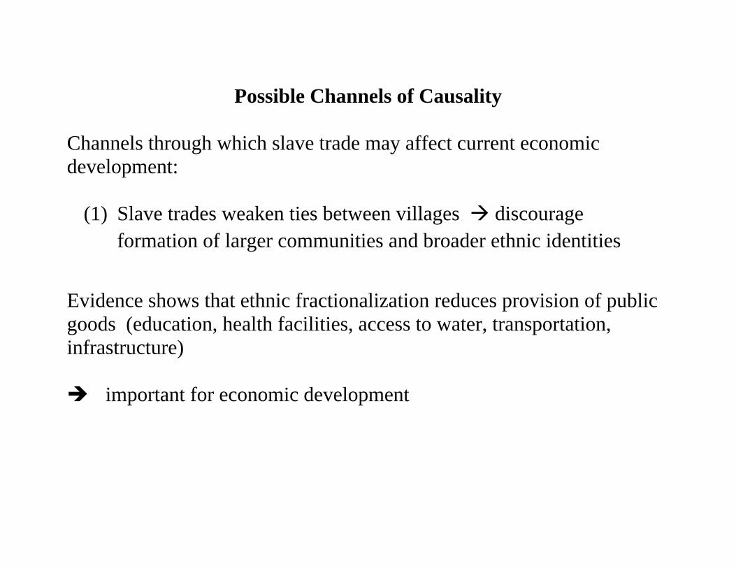
Possible Channels of Causality Channels through which slave trade may affect current economic development:

(1) Slave trades weaken ties between villages discourage formation of larger communities and broader ethnic identities

Evidence shows that ethnic fractionalization reduces provision of public goods (education, health facilities, access to water, transportation, infrastructure) important for economic development


FIGURE VIRelationship between Slave Exports and Current Ethnic Fractionalization

preliminary and exploratory. With only 52 observations it is notpossible to pin down the precise channels and mechanism under-lying the relationships with any reasonable degree of certainty.My strategy here is to simply investigate whether the data areconsistent with the historic events described in Section II.

An important consequence of the slave trades was that theytended to weaken ties between villages, thus discouraging theformation of larger communities and broader ethnic identities. Iexplore whether the data are consistent with this channel by ex-amining the relationship between slave exports and a measureof current ethnic fractionalization from Alesina et al. (2003). Asshown in Figure VI, there is a strong positive relationship be-tween the two variables.18 This is consistent with the historicaccounts of the slave trades impeding the formation of broaderethnic identities.

This consequence of the slave trades is important because ofthe increasing evidence showing that ethnic fractionalization is an

18. The results are also similar if other measures of ethnic fractionalizationare used.

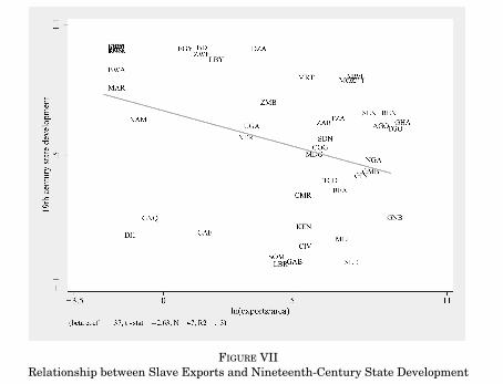
(2) Slave trades weakened and under developed states

negative relationship between slave exports and 19th century state

centralization

Consistent with slave trades causing long-term political instability weakened and fragmented states

undevelopment of political structures (institutions)


FIGURE VIIRelationship between Slave Exports and Nineteenth-Century State Development

growth between 1960 and 1995. Looking within Africa, Gennaioliand Rainer (2006) find that countries with ethnicities that hadcentralized precolonial state institutions today provide more pub-lic goods, such as education, health, and infrastructure.

Herbst (1997, 2000) also focuses on the importance of statedevelopment for economic success, arguing that Africa’s pooreconomic performance is a result of postcolonial state failure,the roots of which lie in the underdevelopment and instability ofprecolonial polities. Herbst (2000, chaps. 2–4) argues that becauseof a lack of significant political development during colonial rule,the limited precolonial political structures continued to exist afterindependence.19 As a result, Africa’s postindependence leadersinherited nation states that did not have the infrastructurenecessary to extend authority and control over the whole country.Many states were, and still are, unable to collect taxes fromtheir citizens, and as a result they are also unable to provide aminimum level of public goods and services.

19. On the continuity between Africa’s precolonial and postcolonial politicalsystems also see Hargreaves (1969, p. 200).

Date post:	27-Mar-2019
Category:	Documents
Upload:	phungphuc
View:	218 times
Download:	0 times

Find measures of institutional performance and economic...

Documents