1 Findings and Recommendations of the Statistical Expert Panel on Central Registry Completeness March 15, 2021 Acknowledgment This publication was supported by the Cooperative Agreement Number 6-NU38OT000286-01 funded by the Centers for Disease Control and Prevention (CDC). Its contents are solely the responsibility of the author and do not necessarily represent the official views of CDC or the U.S. Department of Health and Human Services.
Transcript
1
Findings and Recommendations of the Statistical Expert Panel on Central Registry Completeness
March 15, 2021
Acknowledgment
This publication was supported by the Cooperative Agreement Number 6-NU38OT000286-01 funded by the Centers for Disease Control and Prevention (CDC). Its contents are solely the responsibility of the author and do not necessarily represent the official views of CDC or the U.S. Department of Health and Human Services.
2
Introduction This report contains the findings and recommendations of the Statistical Expert Panel with respect to measuring completeness of case ascertainment at central cancer registries in the United States. One core function of central cancer registries is the publication of population-based incidence rates, which requires that all cases be reported and counted. Evidence suggests that the completeness of case reporting in the United States has improved in the last 10 years. Although it is impossible to know what cases may be missing, delayed reports and reports from death certificates suggest that only a few percent of cases are not reported within the required 23-month time frame nationwide.
For more than a quarter century, completeness has been measured by the North American Association of Central Cancer Registries, Inc., (NAACCR) and the National Program of Cancer Registries (NPCR) in a consistent manner: An expected number of cases is calculated based on cancer mortality rates and adjusted for the demographic structure of each state’s population, and the reported number of cases is compared to this expected number. This report expands on that approach to produce a suite of indicators that are more sensitive to diverse aspects of case reporting.
Statistical methods for estimating case completeness can be classified into two primary types. Internal methods are those that predict case counts based on registries’ own reporting history. External methods are those that predict case counts based on variables that are external to central registries. These include mortality rates, population demographics, socioeconomic indicators, and information from health surveys. Each of these types of methods has its own sets of limitations, some of which are discussed below. To overcome the limitations inherent in each method, the Statistical Expert Panel proposed a solution that makes use of both methods as part of a suite of completeness indicators. For registries that perform well using both methods, there is higher confidence in the completeness of their data than is achieved from using either method on its own. The same is true for registries that do not perform well on either measure. For registries that perform well on one measure but not the other, a set of process measures is proposed to help resolve the discrepancy and assist registries in identifying potential gaps in reporting.
The concept is illustrated in Figure 1, which reports internal and external completeness scores for 56 U.S. registries for cases diagnosed in 2017 and reported in 2019. The plot has been color-coded into zones representing completeness scores above both thresholds (green), one threshold (yellow), and no thresholds (red). The thresholds used here are for illustrative purposes only, although they do correspond to values that have been used historically. Forty-six registries were above both thresholds, one was below both thresholds, and nine were below one threshold and above the other.
3
Figure 1. Internal versus external completeness measures for cases diagnosed in 2017. Each point corresponds to a registry.
One would expect that independent measures of a quantity such as completeness should agree, but the correlation in Figure 1 is quite low. The reason for this is believed to be that the two methods are sensitive to different characteristics of the data. The internal method is sensitive to registries that have a substantial drop in cases in a single year. It is not sensitive to registries that have consistently underreported cases for a number of years. The method looks for adherence to a trend; if the trend is to underreport, then the registry will be adhering to that trend. The external method, in contrast, is sensitive to registries that appear to be underreporting relative to other registries. A registry that does so consistently will be identified as such each year. But because the method assumes the average registry has complete data, it is not sensitive to national trends in reporting. For example, because of the delayed rollout of the coding rules for cases diagnosed in 2018, it is likely that completeness declined nationally, but the threshold is still based on a percentage of the average registry, where the average registry is presumed complete. The lack of agreement between the internal and external measures is the reason additional measures should be taken into consideration when evaluating completeness.
The following sections provide technical detail about the proposed internal, external, and secondary methods.
4
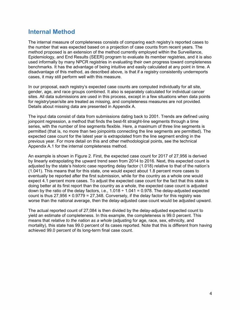
Internal Method The internal measure of completeness consists of comparing each registry’s reported cases to the number that was expected based on a projection of case counts from recent years. The method proposed is an extension of the method currently employed within the Surveillance, Epidemiology, and End Results (SEER) program to evaluate its member registries, and it is also used informally by many NPCR registries in evaluating their own progress toward completeness benchmarks. It has the advantage of being intuitive and easily calculated at any point in time. A disadvantage of this method, as described above, is that if a registry consistently underreports cases, it may still perform well with this measure. In our proposal, each registry’s expected case counts are computed individually for all site, gender, age, and race groups combined. It also is separately calculated for individual cancer sites. All data submissions are used in this process, except in a few situations when data points for registry/year/site are treated as missing, and completeness measures are not provided. Details about missing data are presented in Appendix A. The input data consist of data from submissions dating back to 2001. Trends are defined using joinpoint regression, a method that finds the best-fit straight-line segments through a time series, with the number of line segments flexible. Here, a maximum of three line segments is permitted (that is, no more than two joinpoints connecting the line segments are permitted). The expected case count for the latest year is extrapolated from the line segment ending in the previous year. For more detail on this and other methodological points, see the technical Appendix A.1 for the internal completeness method. An example is shown in Figure 2. First, the expected case count for 2017 of 27,956 is derived by linearly extrapolating the upward trend seen from 2014 to 2016. Next, this expected count is adjusted by the state’s historic case reporting delay factor (1.018) relative to that of the nation’s (1.041). This means that for this state, one would expect about 1.8 percent more cases to eventually be reported after the first submission, while for the country as a whole one would expect 4.1 percent more cases. To adjust the expected case count for the fact that this state is doing better at its first report than the country as a whole, the expected case count is adjusted down by the ratio of the delay factors, i.e., 1.018 ÷ 1.041 = 0.978. The delay-adjusted expected count is thus 27,956 × 0.9779 = 27,348. Conversely, if the delay factor for this registry was worse than the national average, then the delay-adjusted case count would be adjusted upward. The actual reported count of 27,084 is then divided by the delay-adjusted expected count to yield an estimate of completeness. In this example, the completeness is 99.0 percent. This means that relative to the nation as a whole (adjusting for age, race, sex, ethnicity, and mortality), this state has 99.0 percent of its cases reported. Note that this is different from having achieved 99.0 percent of its long-term final case count.
5
Figure 2. Joinpoint model used to derive expected case count in the internal completeness method
External Method The external method of calculating completeness is similar to the internal method in that it compares each registry’s reported cases to an expected number of cases to derive a proportion. The external method, however, uses factors outside the registry’s own data in determining the expected number of cases. This section recalls the current approach for calculating completeness, introduces a new regression-based approach, and touches on some extensions for the new regression approaches that were considered.
Existing Approach. The existing method used by NAACCR and NPCR for measuring completeness is an example of an external method. With this method, the expected count (e.g., expected number of cancers) for a given registry is as follows:
Expected count = �SEER or NPCR reference incidenceUS Mortality � × Local mortality,
where an expected count is calculated separately for each age group, sex, race/ethnic group, and selected cancer sites. These counts are then summed to obtain a single expected count. The ratio of the observed to expected counts is then taken as a measure of completeness. This ratio is multiplied by 100 to obtain a completeness score.
6
Proposed Regression Based Approach. The Statistical Expert Panel explored an alternative regression-based approach for estimating the expected case counts using regression models that can predict the expected number of cancers. For each cancer site, this report effectively proposes estimating the expected count for a given age group, sex, and race/ethnic group by the following model:
where the functions, f, and other details are provided in Appendix A.2. Again, the expected counts are summed across all demographic groups and cancer-sites to obtain a single expected count (𝑌𝑌�), which is then compared with the observed number (𝑌𝑌). The Statistical Expert Panel reports the estimate of completeness, �̂�𝐶 = 100 × 𝑌𝑌/𝑌𝑌�, the corresponding 95 percent confidence interval, and the probability that the true completeness exceeds pre-specified thresholds.
The Statistical Expert Panel considered two modifications to this proposed regression-based approach to improve the prediction of cancer incidence. They first considered using additional demographic and behavioral information about the population in each of the registries. This information—drawn from the American Community Survey (ACS) of the U.S. Census, the Behavioral Risk Factor Surveillance Survey (BRFSS) of CDC, and the Area Health Resources File (AHRF) produced by the Health Resources and Services Administration—was captured in the set of 33 additional variables listed in Appendix A.3. The variables were chosen based on a hypothesized association with cancer incidence or because they have been historically included in similar modeling projects. The ACS and AHRF variables were available at the county level, and the BRFSS variables were available at the state level. Most were not available by age or race/ethnicity categories. For most cancer sites, including these additional variables in the model did not improve the accuracy of the predictions and, therefore, for simplicity the Statistical Expert Panel chose to use the base model described above.
Second, the Statistical Expert Panel considered fitting the regression models using county-level data. Again, this additional level of complexity did not significantly improve the accuracy of the predictions or warrant further consideration.
Given that the proposed external method and existing NAACCR completeness method use the same inputs (mortality, site, age, sex, race/ethnicity) one might expect them to have similar results. Indeed, this is the case. Figure 3 shows a scatterplot of the two methods for the same year of data. The coefficient of determination (R-squared) between the two is 0.64, indicating good agreement. Thus the regression approach can be seen as a generalization of the NAACCR method, one that allows more flexibility to measure the relationships between covariates and incidence rates and that allows a wide array of additional variables to be added.
7
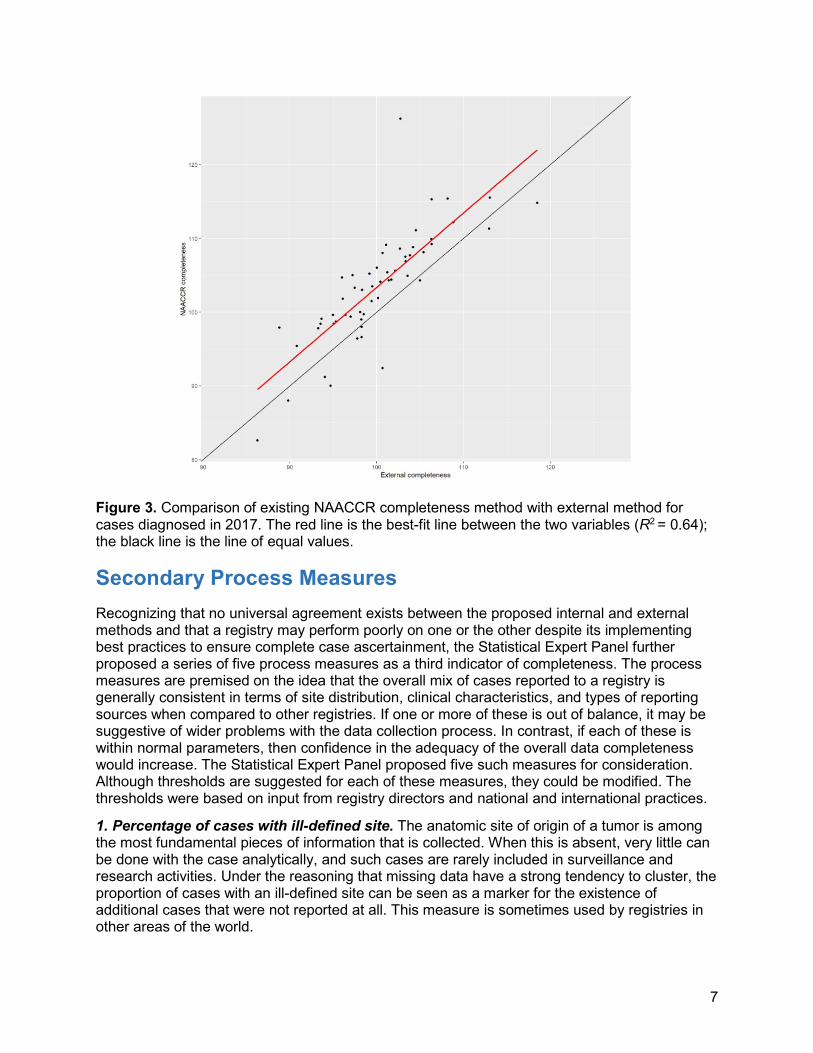
Figure 3. Comparison of existing NAACCR completeness method with external method for cases diagnosed in 2017. The red line is the best-fit line between the two variables (R2 = 0.64); the black line is the line of equal values.
Secondary Process Measures Recognizing that no universal agreement exists between the proposed internal and external methods and that a registry may perform poorly on one or the other despite its implementing best practices to ensure complete case ascertainment, the Statistical Expert Panel further proposed a series of five process measures as a third indicator of completeness. The process measures are premised on the idea that the overall mix of cases reported to a registry is generally consistent in terms of site distribution, clinical characteristics, and types of reporting sources when compared to other registries. If one or more of these is out of balance, it may be suggestive of wider problems with the data collection process. In contrast, if each of these is within normal parameters, then confidence in the adequacy of the overall data completeness would increase. The Statistical Expert Panel proposed five such measures for consideration. Although thresholds are suggested for each of these measures, they could be modified. The thresholds were based on input from registry directors and national and international practices.
1. Percentage of cases with ill-defined site. The anatomic site of origin of a tumor is among the most fundamental pieces of information that is collected. When this is absent, very little can be done with the case analytically, and such cases are rarely included in surveillance and research activities. Under the reasoning that missing data have a strong tendency to cluster, the proportion of cases with an ill-defined site can be seen as a marker for the existence of additional cases that were not reported at all. This measure is sometimes used by registries in other areas of the world.
8
Figure 4 shows that in no registries were more than 3 percent of all cases coded to ill-defined site and in one registry more than 2.5 percent of cases were coded to ill-defined site. The seven yellow points correspond to seven registries under secondary review—that is, they achieved favorable completeness scores based on either the internal or external methods but not on both. These are drawn from the 10 points in the red or yellow zones in Figure 1, after removing three that had a reasonable probability of exceeding the threshold after accounting for uncertainty related to registry size (this is explained further in the Sample Report following this section). In Figure 4, each of these seven points has a typical value relative to other registries. The highest-valued registry here is an outlier, falling outside the whiskers of the box-and-whiskers plot, defined here as exceeding the 75th percentile by more than 1.5 times the interquartile range. The red dashed line at 3 percent indicates a possible threshold for this measure, although 2.5 percent or any value that is an outlier also could be justified.
Figure 4. Proportion of cases with ill-defined site, by registry, 2017 diagnosis. Each point corresponds to a registry. Yellow points represent registries of potential concern as explained in the text.
2. Proportion of myeloma and leukemia cases. Focusing on cancer sites that are known to have a tendency to be underreported or to have substantially delayed reporting can be indicative of more widespread reporting issues. In contrast, if a registry appears to have good reporting for these sites, it is more likely that it has good reporting for all sites. The two major site groupings with the largest delay factors as calculated and published by SEER in recent years are, by far, leukemia and myeloma. For cases diagnosed in 2017 and submitted in 2019, the delay factor for leukemia was 1.13 and myeloma was 1.11, compared with 1.04 for all sites combined. The delay factors for all other individual sites tabulated were between 1.03 and 1.05, with the exceptions of uterus (1.02), prostate (1.06), and liver (1.06). Figure 5 shows the proportion of leukemia and lymphoma cases by registry. The only outlier was a registry with a value just above the proposed threshold of 3 percent, but it was not among the seven registries
9
of concern. This could indicate that this registry is generally complete but one may want to look at the reporting of these two sites more specifically. It is possible, of course, to meet a data completeness standard while being deficient in a specific cancer site. The proportion of myeloma/leukemia also is influenced by the underlying cancer risk in the population. In particular, the registries that tend to be near the bottom of this distribution (those around 4 percent) tend to be those with very high percentages of white populations. This raises the possibility of using race-adjusted proportions rather than absolute proportions, which is not presented here but would be easy to implement.
Figure 5. Proportion of leukemia and myeloma cases, by registry, 2017 diagnosis. Each point corresponds to a registry. Yellow points represent registries of potential concern as explained in the text.
3. Percent of brain tumors with benign behavior. The collective body of years of national cancer data reporting suggest that about 70 percent of all brain tumors are benign (Ostrom et al., 2020). A central registry that deviates too far from this range may have a problem with either benign or malignant tumors’ being underreported. Figure 6 shows one severely outlying registry with a value well below 50 percent and a second registry exactly at the proposed threshold of 55 percent. The latter is among the seven registries of concern. No registries exceed the other proposed threshold of 80 percent. The registry falling below 50 percent, incidentally, has shown this pattern year after year. Again, it may be indicative of a problem with a specific type of reporting that is not sufficient to impact the overall completeness by a large degree.
10
Figure 6. Proportion of brain tumors that are benign, by registry, 2017 diagnosis. Each point corresponds to a registry. Yellow points represent registries of potential concern as explained in the text.
4. Percentage of cases that are microscopically confirmed. Over recent years, approximately 94 percent to 95 percent of all reported cancers have been microscopically confirmed nationally, and this figure exhibits little variation among registries (CDC, 2020). When this value falls far outside of this range, it can indicate potential underreporting of either clinical or pathologic cases. Figure 7 indicates that four registries fell below a proposed threshold of 92 percent, but none of these were among the seven registries of concern, and none qualified as outliers. No registries exceeded the proposed upper-limit threshold of 97 percent.
11
Figure 7. Proportion of tumors microscopically confirmed, by registry, 2017 diagnosis. Each point corresponds to a registry. Yellow points represent registries of potential concern as explained in the text.
5. Proportion of death certificate only (DCO) cases. As proportion DCO cases is already a data certification standard, this measure has a certain redundancy, but its use here is not entirely redundant. Generally speaking, the correlation between DCO proportion and completeness should be high, because death certificates function as a primary backstop to detect missed cases. If a cancer diagnosis is not reported while a patient is alive, it will be reported on the death certificate if that cancer is a primary cause of death, although recommended practice is to also review cases where cancer is listed as a contributing cause of death. This practice does not mean that death certificates pick up all missed cases, but rather that death certificates pick up a substantial proportion of the missed cases. If a DCO rate is unusually high, therefore, in the case of disagreement between the internal and external modeling methods, the balance tips in favor of incomplete reporting. In contrast, a registry with a low DCO rate would be tipped in favor of complete reporting. In Figure 8, two registries are seen to have exceeded the existing standard of 3 percent, neither of which was among the seven registries of concern.
12
Figure 8. Proportion of tumors reported only by death certificate, by registry, 2017 diagnosis. Each point corresponds to a registry. Yellow points represent registries of potential concern as explained in the text.
In addition, we are proposing that there also be a minimum threshold for DCO cases. Occasionally, registries have reported zero or virtually zero DCO cases, which is implausible. (There will always be a very small share of patients who die at home from cancer without ever being treated, for example). We are proposing to set this threshold at 0.1 percent. No registries were near this threshold.
Summary of secondary process measures. Among the seven registries for which there was a suggestion of a problem with reporting completeness because of falling below either the internal or external threshold, all seven met the secondary process measure thresholds, although one was exactly at the proposed threshold for the proportion of brain cancers with benign behavior. Using the logic of our proposed approach, each of these registries would meet the standard for completeness.
13
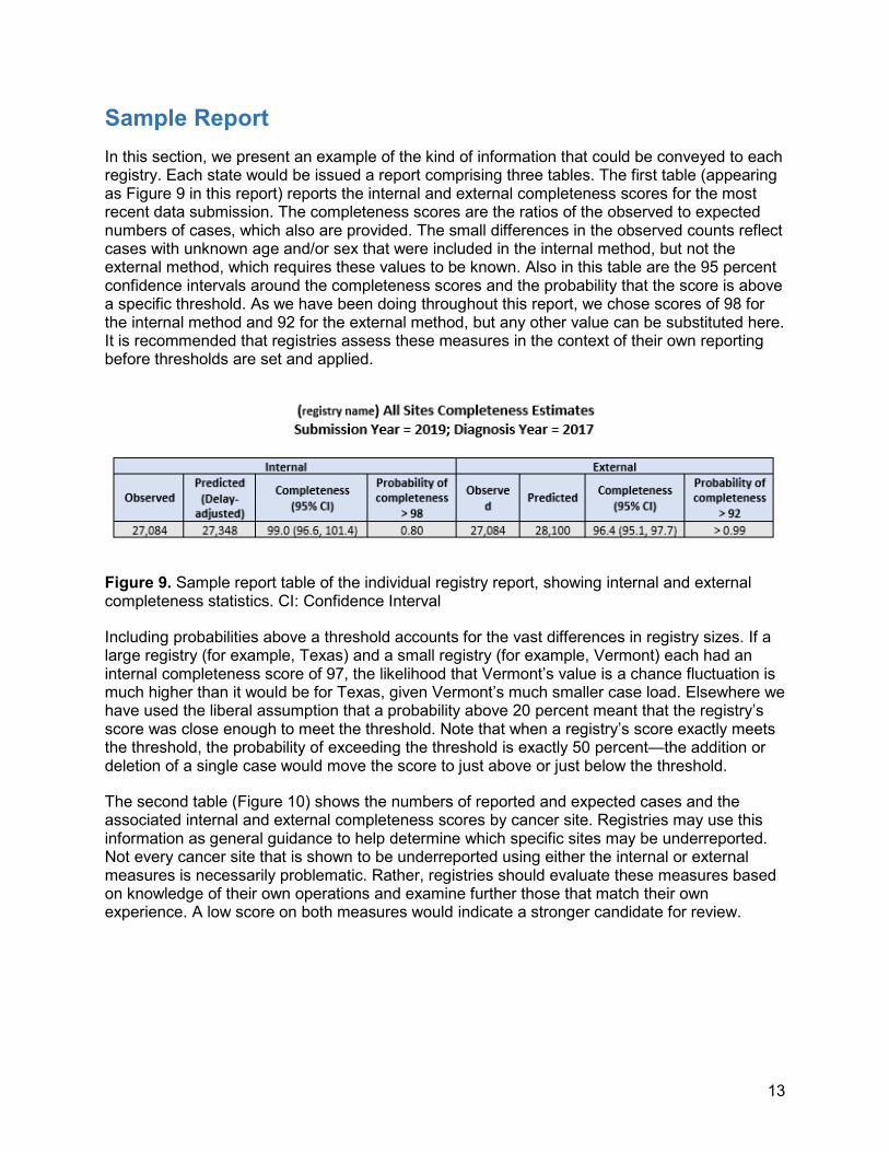
Sample Report In this section, we present an example of the kind of information that could be conveyed to each registry. Each state would be issued a report comprising three tables. The first table (appearing as Figure 9 in this report) reports the internal and external completeness scores for the most recent data submission. The completeness scores are the ratios of the observed to expected numbers of cases, which also are provided. The small differences in the observed counts reflect cases with unknown age and/or sex that were included in the internal method, but not the external method, which requires these values to be known. Also in this table are the 95 percent confidence intervals around the completeness scores and the probability that the score is above a specific threshold. As we have been doing throughout this report, we chose scores of 98 for the internal method and 92 for the external method, but any other value can be substituted here. It is recommended that registries assess these measures in the context of their own reporting before thresholds are set and applied.
Figure 9. Sample report table of the individual registry report, showing internal and external completeness statistics. CI: Confidence Interval
Including probabilities above a threshold accounts for the vast differences in registry sizes. If a large registry (for example, Texas) and a small registry (for example, Vermont) each had an internal completeness score of 97, the likelihood that Vermont’s value is a chance fluctuation is much higher than it would be for Texas, given Vermont’s much smaller case load. Elsewhere we have used the liberal assumption that a probability above 20 percent meant that the registry’s score was close enough to meet the threshold. Note that when a registry’s score exactly meets the threshold, the probability of exceeding the threshold is exactly 50 percent—the addition or deletion of a single case would move the score to just above or just below the threshold.
The second table (Figure 10) shows the numbers of reported and expected cases and the associated internal and external completeness scores by cancer site. Registries may use this information as general guidance to help determine which specific sites may be underreported. Not every cancer site that is shown to be underreported using either the internal or external measures is necessarily problematic. Rather, registries should evaluate these measures based on knowledge of their own operations and examine further those that match their own experience. A low score on both measures would indicate a stronger candidate for review.
14
Figure 10. Sample report table of individual registry report showing internal and external observed and expected cases by site. ONS: Other Nervous System, NOS: Not otherwise specified, IBD: Intrahepatic bile duct.
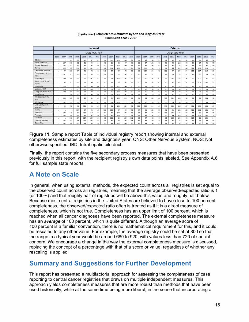
The third table (Figure 11) shows internal and external completeness scores by site and year. This table is intended to assist registries in getting a sense of how their reporting has performed over time.
15
Figure 11. Sample report Table of individual registry report showing internal and external completeness estimates by site and diagnosis year. ONS: Other Nervous System, NOS: Not otherwise specified, IBD: Intrahepatic bile duct.
Finally, the report contains the five secondary process measures that have been presented previously in this report, with the recipient registry’s own data points labeled. See Appendix A.6 for full sample state reports.
A Note on Scale In general, when using external methods, the expected count across all registries is set equal to the observed count across all registries, meaning that the average observed/expected ratio is 1 (or 100%) and that roughly half of registries will be above this value and roughly half below. Because most central registries in the United States are believed to have close to 100 percent completeness, the observed/expected ratio often is treated as if it is a direct measure of completeness, which is not true. Completeness has an upper limit of 100 percent, which is reached when all cancer diagnoses have been reported. The external completeness measure has an average of 100 percent, which is quite different. Although an average score of 100 percent is a familiar convention, there is no mathematical requirement for this, and it could be rescaled to any other value. For example, the average registry could be set at 800 so that the range in a typical year would be around 680 to 920, with values less than 720 of special concern. We encourage a change in the way the external completeness measure is discussed, replacing the concept of a percentage with that of a score or value, regardless of whether any rescaling is applied.
Summary and Suggestions for Further Development This report has presented a multifactorial approach for assessing the completeness of case reporting to central cancer registries that draws on multiple independent measures. This approach yields completeness measures that are more robust than methods that have been used historically, while at the same time being more liberal, in the sense that incorporating a
16
broader set of criteria makes it less likely that a registry will be incorrectly identified as having data that is insufficiently complete.
These measures were presented to a cross-section of NPCR registries on December 21, 2020, to a positive reception. Our recommendation is that all NPCR-funded registries be given time to evaluate the proposed approach in depth and assess the implications for their own data before proceeding with any implementation. NAACCR plans to work closely with registries and the NPCR program to help registries explore these measures.
Once again, note that the various cutoffs and threshold values included here are for illustration only and include a mixture of values that have been used historically and others that have not been. The focus should not be on these threshold values but rather on the methods that generated them. After these indicators have been evaluated fully by the surveillance community, we may begin to discuss the utility and benefit of establishing common thresholds. In reviewing their reports, registries should consider each of the measures, even where they seem to contradict.
Over the long term, the delay factor is a quite good estimate of completeness. That the national delay factor at the 24-month submission point for all sites combined is about 1.04 means that registries were about 96 percent complete at the time of submission, assuming all cases were eventually reported. Obviously, because some cases will never be reported, this 96 percent represents an overestimate, but not a particularly large one. Registries employ many processes to capture delinquent cases and have a good sense based on decades of experience of where problems lie. It may not seem possible to quantify the never-reported cases, but this is not an uncommon problem in science. The field of wildlife ecology, for example, is routinely tasked with the problem of estimating a population size based only on limited sightings of animals, and a rich methodological literature exists around this problem.
Assume that after taking this into consideration, the average registry completeness at the time of 24-month submission ticks down to 95 percent. The question, then, is how to identify which registries are well below that. We obviously cannot wait 4 or more years to get the answer by seeing how the late cases trickle in. In fact, it would be nice to know this even sooner than 24 months, if possible. (Appendix A.4 discusses the implication of looking at data completeness after 12 months). One way to tackle this problem would be to take a deep dive into a large and representative sample of cases that were reported after 2 years to ascertain the pathways and mechanisms by which this happened. Are facilities sending in their cases years after the due date, are these cases coming from nontraditional reporting sources, are they coming out of suspense files within registries themselves because of past data quality issues or because of an oversight, are they patients who lived in multiple states or countries? Such a deep dive would not only help better predict what an initial completeness score might be, but also give registries immediate guidance in how to attack these problems at the present moment. An analysis of this type was not possible with a team comprising members not affiliated with central registries, with no access to this level of data. But it is something that could be undertaken within the existing NAACCR volunteer structure.
With respect to the methods described in this document, opportunities exist to refine them further. For example, in the external method, although no additional census or BRFSS or AHRF variables were found to significantly improve the model globally, it may be the case that additional variables would help on a site-specific basis. For example, there was some indication that one or more socioeconomic variables improved the predictions of breast cancer. For the secondary process measures, it may be possible to develop additional site-specific measures
17
beyond the ones proposed here for leukemia/myeloma and brain cancer. As with most aspects of our field, the models and methods are ever-changing, and the topic of data completeness should continue to be viewed as dynamic rather than closed. Increased emphasis on ensuring that registries are carrying out processes that increase confidence in the completeness of their data is warranted.
References
Centers for Disease Control and Prevention. 2020. Diagnostic confirmation, U.S. Data (2001-). Accessed February 26, 2021. https://www.cdc.gov/cancer/uscs/public-use/dictionary/diagnostic-confirmation.htm
Ostrom QT, Patil N, Cioffi G, Waite K, Kruchko C, Barnholt-Sloan JS. CBTRUS Statistical Report: Primary brain and other central nervous system tumors diagnosed in the United States in 2013–2017. Neuro-Oncology 2020; 22(1): Supplement.
The Statistical Expert Panel comprised a broad-based constituency including thought leaders in biostatistics of cancer surveillance. Members include the following:
Frank Boscoe, Ph.D., Pumphandle, LLC Eric J Feuer, Ph.D., Li Zhu, Ph.D., NCI Joshua Sampson, Ph.D., NCI Trevor Thompson, CDC Joe Zhou, IMS
Additional Contributors—NAACCR staff and consultants and registry directors.
Special thanks to Rocky Feuer, Li Zhu, and Joshua Sampson of NCI who donated countless in-kind hours to this project. Please note that the opinions and recommendations expressed here are not intended to reflect policy of the NCI SEER Program.
18
Appendix A: Completeness Statistical Report
19
Appendix A.1 Internal Method Case and Geography Definition. The internal method uses cases with International Classification of Diseases (ICD)-O-3 behavior codes of malignant, malignant only in ICD-O-3, and only malignant 2010+. The same behavior codes are used in the external method. The small differences in the two are because the external method requires age and sex to be known and excludes those cases with missing values for either of these variables. The cases on all cancer sites combined and 20 individual cancer sites are taken as input to the model described below. The Joinpoint model and delay adjustment are applied separately for all sites combined and for each of the individual sites. Unlike in the external model, we do not sum the completeness measures of individual sites to get the measure of all sites combined. Expected case counts are computed for all state registries, plus the District of Columbia, Detroit, Seattle, the three California substate registries, and Puerto Rico, for a total of 57.
Joinpoint. Joinpoint Trend Analysis Software (https://surveillance.cancer.gov/joinpoint/) is a statistical software developed by the National Cancer Institute that models time trends where several different line trends are connected at “joinpoints.” This project has 16 input data points representing diagnosis years 2001 through 2016. We allow up to three time trends (two joinpoints) in these data, where the initial (starting in 2001) and final (ending in 2016) trends must contain at least three points and the middle trend must contain at least four time points. We used the last four years’ (2013–2016) average annual percent change (AAPC) to project one year ahead to 2017. AAPC is a weighted average of the trend coefficients of the underlying joinpoint model, with weights proportional to the length of each trend segment. In the case of a sudden increase or drop during the last trend segment, using AAPC helps to alleviate the abrupt change and provides a smoother projected value.
Delay Adjustment. The expected number of cases is adjusted by the ratio of a registry’s own delay factor to that of the nation. The motivation is to credit the registries with below-average delay factors for the timeliness of their case reporting. In 2017, the nationwide delay factor across all cancer sites was 1.04. Any registry with a delay factor of less than 1.04 will get a reduced expected count than that projected in Joinpoint, hence a higher completeness percent. The delay adjustment is applied for all sites combined and for each of the individual cancer sites. If a registry or a site does not have a specific delay factor, then the adjustment is not applied for the specific registry/site combination.
The projected count from Joinpoint is adjusted by the delay factors as follows:
where Delay-adjustment factor = Registrydelayfactor
Nationaldelayfactor
The completeness measure is then calculated as:
Completeness =Observedcasecount
Delay− adjustedexpectedcount× 100
Evaluation of Completeness for the Current Year and Prior Years. The most recent cases were reported in 2019 for diagnosis years 2017 and before, with 2 years or longer in reporting delay. Every year, North American Association of Central Cancer Registries (NAACCR)
certificates the central registries based on data qualities, of which completeness is an important criterion. To evaluate the diagnosis (Dx) 2017 completeness, the case count from the 2019 submission was the observed count, and the expected count was modeled through joinpoint regression and adjusted for delay factors (described below) using all 2-year delay case counts from Dx 2001 (reported 2003) through Dx 2016 (reported 2018). In the 2019 data submission, all prior years’ data also are supplemented with new cases, and completeness measures are assessed for fit for use. Prior years’ completeness measures are evaluated with previous reporting years’ submissions, with longer reporting delays. For example, with the data submission in 2019 for Dx 2016 data, there is a 3-year reporting delay. All observed counts for Dx 2001 (report 2004 with a reporting delay of 3 years) through Dx 2015 (reported 2018) are put into the joinpoint model. The earliest completeness we can evaluate with this method is for Dx 2006, with a 13-year reporting delay. One less data point is put into the trend for each successive delay because the trends start with diagnosis year 2001. The maximum number of joinpoints is reduced in accordance with the default algorithms used in the Joinpoint software. Uncertainty Measure. In addition to the point estimate of the completeness measure, we also estimate the variance of the completeness measure. Because completeness is the ratio of the observed to the expected counts, we need to consider the uncertainty measure in both the numerator and the denominator and apply the delta method to estimate the uncertainty in the ratio. The numerator in the ratio —the observed count (𝑂𝑂) — is assumed to follow a Poisson distribution with mean 𝜇𝜇. The denominator — the delay-adjusted expected count (W) — is the joinpoint-projected count multiplied by the delay-adjustment factor described above. The variance estimate of the denominator is the square of the delay-adjustment factor multiplied by the variance of the joinpoint projection. Both the mean 𝐸𝐸(𝑊𝑊) and the variance 𝑉𝑉𝑉𝑉𝑉𝑉(𝑊𝑊) of the projection are estimated by the Joinpoint software.
We then apply the delta method to estimate the variance of the ratio of the observed count over the delay-adjusted expected count as:
𝑉𝑉𝑉𝑉𝑉𝑉 �𝑂𝑂𝑊𝑊� = 1
[𝐸𝐸(𝑊𝑊)]2 𝑉𝑉𝑉𝑉𝑉𝑉(𝑂𝑂) + 𝜇𝜇2
[𝐸𝐸(𝑊𝑊)]4 𝑉𝑉𝑉𝑉𝑉𝑉(𝑊𝑊). The variance of W, the joinpoint projected count, is calculated using the following procedure: Let Y = log(W), so Y is the logarithm transformation of W. Case 1: AAPC ≥ 0 and AAPC = last segment’s annual percent change (APC)
𝑌𝑌 = 𝑌𝑌�𝑘𝑘
Notation: 𝑥𝑥 = k-year ahead location. For example, x = 2017, the last segment starting from Dx 2010, ending at Dx 2016. Then 𝑥𝑥1, … , 𝑥𝑥7 = 2010, … ,2016, and �̅�𝑥 = 2013,𝑛𝑛 = 7. Suppose the slope of the last segment is 𝛽𝛽, then
where 𝜎𝜎2 estimated by mean squared error (MSE) and 𝑉𝑉𝑉𝑉𝑉𝑉(𝛽𝛽) is estimated by 𝑆𝑆𝐸𝐸(𝛽𝛽)2. Note that MSE and 𝑆𝑆𝐸𝐸(𝛽𝛽) are found in the Joinpoint output, both based on the log-scale 𝑌𝑌.
21
Case 2: AAPC ≥ 0 and AAPC ≠ last segment’s APC
𝑌𝑌 = 𝑌𝑌�𝑘𝑘
The 4-year AAPC is between Dx 2013 and Dx 2016. Suppose the location at Dx 2013 is 𝑥𝑥𝑎𝑎 and the location at Dx 2016 is 𝑥𝑥𝑏𝑏. The corresponding fitted values are 𝑌𝑌�𝑎𝑎 and 𝑌𝑌�𝑏𝑏 , respectively. The variance of Y is then
𝑉𝑉𝑉𝑉𝑉𝑉(𝑌𝑌) = 𝜎𝜎2 + 𝑉𝑉𝑉𝑉𝑉𝑉�𝑌𝑌�𝑏𝑏� + 𝑘𝑘
2
9�𝑉𝑉𝑉𝑉𝑉𝑉�𝑌𝑌�𝑏𝑏� + 𝑉𝑉𝑉𝑉𝑉𝑉�𝑌𝑌�𝑎𝑎�� + 2𝑘𝑘
3 𝑉𝑉𝑉𝑉𝑉𝑉�𝑌𝑌�𝑏𝑏�
𝑉𝑉𝑉𝑉𝑉𝑉�𝑌𝑌�𝑏𝑏� = 𝜎𝜎2 �1𝑛𝑛
+(𝑥𝑥𝑏𝑏 − �̅�𝑥)2
∑(𝑥𝑥𝑖𝑖 − �̅�𝑥)2� =𝜎𝜎2
𝑛𝑛+ 𝑉𝑉𝑉𝑉𝑉𝑉(𝛽𝛽𝑏𝑏)(𝑥𝑥𝑏𝑏 − �̅�𝑥)2
𝑉𝑉𝑉𝑉𝑉𝑉�𝑌𝑌�𝑎𝑎� = 𝜎𝜎2 � 1𝑚𝑚
+ (𝑥𝑥𝑎𝑎−�̅�𝑧)2
∑(𝑧𝑧𝑖𝑖−�̅�𝑧)2� = 𝜎𝜎2
𝑚𝑚+ 𝑉𝑉𝑉𝑉𝑉𝑉(𝛽𝛽𝑎𝑎)(𝑥𝑥𝑎𝑎 − 𝑧𝑧̅)2,
where 𝑥𝑥1, … , 𝑥𝑥𝑛𝑛 are the last segment; 𝑧𝑧1, … 𝑧𝑧𝑚𝑚 are the segment where 𝑥𝑥𝑎𝑎 is located; 𝛽𝛽𝑏𝑏 is the slope of the last segment; 𝛽𝛽𝑎𝑎 is the slope of the segment, where 𝑥𝑥𝑎𝑎 is located; and �̅�𝑥 is the mean of 𝑥𝑥1, … , 𝑥𝑥𝑛𝑛. 𝑧𝑧̅ is the mean of 𝑧𝑧1, … , 𝑧𝑧𝑚𝑚. Also, 𝜎𝜎2 is estimated by MSE. 𝑉𝑉𝑉𝑉𝑉𝑉(𝛽𝛽𝑎𝑎) is estimated by 𝑆𝑆𝐸𝐸(𝛽𝛽𝑎𝑎)2. 𝑉𝑉𝑉𝑉𝑉𝑉(𝛽𝛽𝑏𝑏) is estimated by 𝑆𝑆𝐸𝐸(𝛽𝛽𝑏𝑏)2. 𝐸𝐸�𝑌𝑌�𝑎𝑎� is estimated by 𝑌𝑌�𝑎𝑎 ,𝐸𝐸�𝑌𝑌�𝑏𝑏� is estimated by 𝑌𝑌�𝑏𝑏. Case 3: AAPC < 0, then 𝑌𝑌 = 𝑌𝑌�0. To predict x = 2017. If the location at Dx 2016 is 𝑥𝑥𝑏𝑏,
𝑉𝑉𝑉𝑉𝑉𝑉(𝑌𝑌) = 𝜎𝜎2 �1 +1𝑛𝑛�
+ 𝑉𝑉𝑉𝑉𝑉𝑉(𝛽𝛽)(𝑥𝑥𝑏𝑏 − �̅�𝑥)2,
where 𝑥𝑥1, … , 𝑥𝑥𝑛𝑛 are the last segment and �̅�𝑥 is the mean of 𝑥𝑥1, … , 𝑥𝑥𝑛𝑛. Once the variance of Y is obtained, we then use the delta method to find the variance of W by
𝑉𝑉𝑉𝑉𝑉𝑉(𝑊𝑊) ≈ 𝑉𝑉𝑉𝑉𝑉𝑉(𝑌𝑌) × (𝑒𝑒𝑥𝑥𝑒𝑒(𝑌𝑌))2.
Probability the Completeness is Greater Than a Cutoff Point. The completeness measure is assumed to follow a normal distribution. Once the point estimate and the variance estimate of the completeness measure are available, we can calculate the probability that the completeness measure of a registry exceeds a desired threshold value of 98 percent. Then, we are able to identify registries with low probabilities of exceeding the threshold, less than 0.2 or 0.4. This approach incorporates the higher variability in data from smaller registries and minimizes any bias in the completeness measure due to registry size.
Missing Data. Not all registry/year/site combinations are presented. In the following four situations, the data are not included as input:
1. For diagnosis year 2005, for all reporting years, Alabama, Louisiana, Mississippi, and Texas only reported about half of the cases due to hurricane Katrina and were excluded.
2. Some of the zeros were obviously wrong in the database; therefore, we removed all of the them. Some true zeros also were removed. The assumption is that they will be removed in the next step if not here.
22
3. Joinpoint was run if there were more than five data points and the mean number of observations was at least 50. If there were less than five data points or if the average count across years was less than 50, then there was no Joinpoint model estimate.
4. Some data points were detected as outliers and, hence, were excluded from the data input. In the case where the outlier exclusion resulted in less than five input points or less than 50 average counts, there was no Joinpoint model estimate. The details of outlier detection are described in the next section.
Outlier Detection. In reviewing the joinpoint trend plots of the case counts and expected counts, we found some registries had an “outlier” year during the 16-year period when the observed counts were either too high or too low relative to the joinpoint estimate. Because these outliers bias the overall time trends, we developed a metric to detect outliers and remove them from the trend calculations. The metric is a nonparametric version of the goodness-of-fit measure. Specifically, it is the ratio of the residual (the difference in the log-transformation between the observed and the estimated counts) over the median of the residual. This ratio has been shown to follow a standard normal distribution. Any data point with a ratio below −2 or above 2 was deemed to be an outlier and was removed from the input data. Joinpoint was then rerun after the removal of the outliers. If the last data point in the joinpoint model is removed as an outlier, then a 2-year projection is applied to get the projected count for the completeness calculation. The resulting joinpoint models thus are unbiased with respect to the outliers.
23
Appendix A.2 External method Case and Geography Definition. The external method uses cases with ICD-O-3 behavior codes of malignant, malignant only in ICD-O-3, and only malignant 2010+. The same behavior codes are used in the internal method. The small differences in the two are because the external method requires age and sex to be known and excludes those cases with missing values for either of these variables. Expected case counts are computed for all state registries, plus the District of Columbia, Detroit, Seattle, and the three California sub-state registries, for a total of 56. Puerto Rico presently is not included in the external method because race information is missing; if all cases are taken to be Hispanic, then this can be computed, but this decision was not reached before the time of this report.
B1. Here, we offer the details on the regression approach. We build nearly 40 regression models. Specifically, we build separate regression models for each cancer type and gender pair (e.g., lung cancer in women). For building each model, we start with a data set that includes the cancer incidence and covariates for each combination of cancer registry, age group, race/ethnicity, reporting year, and calendar year. Because we have 56 registries, 10 age groups (0–4, 5–14, … 75–84, 85+); four race/ethnicity categories (White, Black, Hispanic, and other); five reporting years (2015–2019); and 13 calendar years prior to each reporting year, each data set has approximately 56 × 10 × 4 × 5 × 13 = 145,600 observations. This value may grow as we add additional registries. We then build a regression model to predict cancer incidence using this data set as described next.
Let k index the gender/cancer-type pairing and i index the 145,600 observations within that data set. Let Yki denote the number of cancers, 𝜆𝜆𝑘𝑘𝑖𝑖 = E[𝑌𝑌𝑘𝑘𝑖𝑖], nki denote the population size, {Aki2,…,Aki10} denote age groups, {Rki2 Rki3, Rki4} denote race/ethnicity, {Cki2,…,Cki5} denote calendar year, and {Dki2, …, Dki13} denote reporting delay. Finally, let {Mki1, …, Mki4} be a set of variables that represent log-mortality, which are derived using a natural spline with knots at the 20th, 50th, and 80th percentiles of the positive values. We then fit the following model using Poisson regression with a robust variance estimator.
After fitting equation (2) separately for each of the approximately 40 data sets, we then can estimate the expected cancer rates for a given registry, calendar year, and delay period by 𝑌𝑌� = ∑ ∑ �̂�𝜆𝑘𝑘𝑖𝑖𝑖𝑖∈Ω𝑘𝑘 = ∑ ∑ 𝑛𝑛𝑖𝑖𝑒𝑒𝑥𝑥𝑒𝑒(�̂�𝛽𝑘𝑘𝑋𝑋𝑘𝑘𝑖𝑖)𝑖𝑖∈Ω𝑘𝑘 , where Ω indexes the relevant observations. Letting 𝑌𝑌 = ∑ ∑ 𝑌𝑌𝑘𝑘𝑖𝑖𝑖𝑖∈Ω𝑘𝑘 denote the total number of observed cases, we estimate completeness as �̂�𝐶 = 100 × 𝑌𝑌/𝑌𝑌�. We can calculate the standard error (SE) using the delta method (Appendix A.2). Therefore, we report the 95 percent confidence interval as �̂�𝐶 ± 1.96𝑆𝑆𝐸𝐸 and the probability of exceeding a prespecified threshold, c, by P(Z > c), where Z ~ N(�̂�𝐶,SE2).
We considered two modifications to model 2. First, we considered including additional covariates (e.g., smoking rates, poverty levels, obesity rates),
where {Wki1,…,Wkip} are the p additional variables relevant for the kth gender and cancer pair (i.e., not all 33 variables will be relevant for each cancer type). Second, we considered using county-level data. The data sets now would include cancer incidence for each combination of county (as opposed to cancer registry), age group, race/ethnicity, reporting year, and delay year. Given that approximately 3,000 counties are in the United States, each data set includes approximately 3,000 × 10 × 4 × 5 × 13 = 7,800,000 observations.
B2. We can obtain the SE for the external estimate of completeness �̂�𝐶. Referring to equation 2, we assume that √𝑁𝑁(�̂�𝛽𝑘𝑘 − 𝛽𝛽𝑘𝑘) ∼ 𝑁𝑁(0,𝛴𝛴𝑘𝑘), let 𝛴𝛴�𝑘𝑘 be the robust variance estimator, and denote the needed derivatives by
Moreover, letting 𝜎𝜎�𝑘𝑘𝑘𝑘2 =∑ Y𝑘𝑘𝑖𝑖𝑖𝑖∈Ω , �̂�𝜆𝑘𝑘 = ∑ 𝑛𝑛𝑖𝑖𝑒𝑒𝑥𝑥𝑒𝑒(�̂�𝛽𝑘𝑘𝑋𝑋𝑘𝑘𝑖𝑖)𝑖𝑖∈Ω , �̂�𝜆 = ∑ �̂�𝜆𝑘𝑘𝑘𝑘 , 𝜎𝜎�𝐸𝐸2 = ∑ 𝜎𝜎�𝑘𝑘𝐸𝐸2𝑘𝑘 , and 𝜎𝜎�𝑘𝑘2 = ∑ 𝜎𝜎�𝑘𝑘𝑘𝑘2𝑘𝑘 , we estimate the distribution of completeness by
(�̂�𝐶 − C) ∼ 𝑁𝑁(0, (�̂�𝐶2𝜎𝜎�𝐸𝐸2 + 𝜎𝜎�𝑘𝑘2)/�̂�𝜆2) ≡ 𝑁𝑁(0,𝜎𝜎�𝑘𝑘2).
25
Appendix A.3. List of Additional Variables Considered for External Method Age and Sex Percentage of persons under 18 years of age Percentage of persons 65 years and over Percentage of female-headed households Education Percentage of persons 25 years and over with at least a bachelor’s degree Percentage of persons 25 years and over with less than 9th grade education Employment Percentage of persons 16 years and over who are unemployed Percentage of white collar workers Income Median household income Percentage of families below poverty Percentage of persons below poverty Geography Land area in square miles Population density Percentage of persons in rural areas Percent migrating between states Housing Percentage of households with more than one person per room Language Percentage of households that is isolated linguistically Race/Ethnicity/National Origin Percent Hispanic Percent foreign born Percent non-Hispanic American Indian and Alaska Native alone Percent non-Hispanic Black alone Percent non-Hispanic White alone Cancer Outcomes Relative survival Health Behaviors Percentage of adults with a body mass index greater than 25 Percentage of females who ever smoked Percentage of males who ever smoked
26
Health Insurance Percentage of females less than 65 years without insurance Percentage of males less than 65 years without insurance Medical Care and Screening Hospitals per 1,000 population Doctors per 1,000 population Percentage of individuals meeting age-appropriate colorectal cancer-screening guidelines Percentage of women meeting age-appropriate breast cancer-screening guidelines Percentage of women meeting age-appropriate cervical cancer-screening guidelines Percentage of men over age 50 years receiving a prostate-specific antigen test in the past year
27
Appendix A.4 Potential Use of January (12-month) NAACCR Submissions for Reporting National Cancer Statistics The data submitted to NAACCR in November is used to report cancer statistics for cases diagnosed through 2 years earlier. For example, the November 2020 submission will be used to produce statistics diagnosed through the end of 2018. This data submission also is known as 24-month data because the time between the submission and 2 years earlier is 24 months. Since 2013, NPCR-funded registries have made a second submission to produce the first report on cases diagnosed through the previous year. This submission is due in January, but many registries submit it at the same time because their other submission is due in November. This is known as 12-month data, although given the range of submission times, it is technically 11- to 13-month data. With an interest in making population-based cancer registry reporting more timely, a natural question is whether the 12-month data are complete enough for the reporting of national cancer statistics.
To answer this question, it is useful to look at the experience of SEER registries. Since 2011, SEER registries have been making their second submission in February, one month later than NPCR registries, effectively making it 14-month data, although it often is referred to as 12-month data as well. After the first four such submissions, an article was published titled “Early estimates of SEER cancer incidence for 2012: approaches, opportunities, and cautions for obtaining preliminary estimates of cancer incidence” (Cancer 2015; 121(12): 2053-2062). This paper found that although fewer cases were reported in the February submissions than in the subsequent November submissions, the amount of under-reporting was not that large and was fairly consistent over time. This allowed the authors to adjust for the under-reporting of rates from the February submissions by extending the reporting delay model, which had been previously used for November submissions.
Reporting delay factors represent a multiplier by which rates should be adjusted to account for additional cases that will come in eventually. For example, a factor of 1.05 means that the rates should be adjusted upward by 5 percent. For SEER November submissions, reporting delay factors range from about 1.025 to 1.15 depending on the cancer site, with the largest factors for leukemia, lymphoma, and myeloma. For the SEER February submissions, the factors are usually about twice as large, ranging from about 1.05 to 1.30. They also found that Joinpoint trends estimated using the February submission were very close to trends estimated using the subsequent November submission. This analysis provided confidence that preliminary estimates of rates and trends could be released earlier than the typical delay of 28 months (23 months for reporting and then an additional 5 months for processing before being released in April. National Cancer Institute published preliminary rates and trends in the journal Cancer for the next 3 years (122(10): 1579-1587, 123(13): 2524-2534, 124(10): 2192-2204) and on the SEER website in 2019 (https://seer.cancer.gov/statistics/preliminary-estimates/).
For these estimates to be valid, there must be consistency in the under-reporting over time because the delay model uses the history of reporting delays to predict future delays. For example, the February 2020 submission, including cases diagnosed through 2018, was thought to be more under-reported than prior February submissions due to delays in the release of updated coding software to registries. Consequently, no preliminary estimates were published this year.
To evaluate the potential of using NAACCR submissions to produce preliminary rates and trends, we computed the ratio of cancer counts by registry for the January to subsequent
November submissions for selected cancer sites for submissions in 2013, 2014, 2015, and 2016. They are displayed for all sites, colon and rectum, female breast, lung, and prostate cancers in Figures 12 through 16. Each of the 69 registries that submitted data to NAACCR, including Canadian registries, is displayed in a column with a dot for each of the four ratios, sorted by the 2013 ratio. Registries were assigned random reference codes to prevent identification. The figures allow one to view the average level of the ratios for each registry, as well as their variability, which as previously described is a key to estimating delay factors with reasonable predictive ability. Missing data points indicate missing 12-month submissions and/or subsequent 24-month submissions that did not meet minimum NAACCR certification standards. We chose a ratio of 0.8 as an ad hoc cut point for ratios sufficiently high for delay modeling, requiring that registries met this threshold in at least 3 of the 4 years. Thirty-three registries met this threshold for all sites combined, and 36 met this threshold for colorectal and breast cancers, but only 24 reached the threshold for lung and bronchus cancer and 23 for prostate cancer. The reasoning behind the choice of 0.8 is as follows: Assume that these each of these cancers had an average reporting delay factor of 1.05 based on the subsequent November submission, making the ratio of the cases from that submission to the final count years later 1 ÷ 1.05 = 0.95. Then, a 12- to 24-month ratio of 0.8 translates to a delay factor of 1 ÷ (0.8 × 0.95) = 1.3, which is among the largest delay factors for the SEER February submissions. Note that delay factors for cancers beyond these most common sites may be substantially larger.
Further evaluation would be necessary to determine whether the rates or trends from the 12-month NPCR submission could be utilized reliably. The ratios in Figures 12 through 16 should be updated to include data for 2017–2020. The delay model then could be run for registries where a majority of the ratios are greater than 80 percent. Similar to what was done with the SEER registries, evaluations should be conducted to determine how well the 12-month delay-adjusted rates and joinpoint trends track the 24-month delay-adjusted rates and joinpoint trends. Depending on these results, a stricter registry inclusion threshold than 0.8 may be necessary. These preliminary results show some promise for early reporting but only for roughly half of all registries.
29
Appendix A.5 Completeness Estimates
All Sites Completeness Estimates Submission Year = 2019; Diagnosis Year = 2017