Fine HVAC

Quick Start Guide

1. Installation – Launching

2. CAD Environment

3. Calculation Environment

Preface This Quick Start Guide provides a fast and friendly introduction on Fine HVAC main features and functionalities.

Fine HVAC, the Fully INtegrated Environment for Heating, Ventilation and Air-Conditioning Installations combines both designing and calculations in a uniform, integrated environment, consisting of two main components, CAD and Calculations:

Concerning the CAD component, it is based on an autonomous CAD embedding 4MCAD engine adopting the common cad functionality and open dwg drawing file format. The CAD component helps the user to design and then calculates and produces completely automatically the entire calculations issue for every HVAC project, as well as all the drawings in their final form.

Concerning the Calculations component (called also as ADAPT/FCALC), it has been designed according to the latest technological standards and stands out for its unique user - friendliness, its methodological thoroughness of calculations and its in-depth presentation of the results. The HVAC Calculation Environment consists of 8 modules: Heating Loads, Single Pipe System, Twin Pipes System, Infloor System, Cooling Loads, Fan Coils, Air Ducts and Psychrometrics. Each module acquires data directly from the drawings (automatically), thus resulting in significant time saving and maximum reliability of the project results. It can also be used independently, by typing data within the module spreadsheets.

Despite its numerous capabilities, Fine HVAC has been designed in order to be easy to learn. Indeed, the simplicity in the operation philosophy is realised very soon and all that the user has to do is to familiarise with the package.

This Guide is divided into three short parts:

- Part 1 describes the installation procedure and the main menu structure. - Part 2 deals with the CAD component of Fine HVAC, showing its philosophy and main

features. - Part 3 describes the calculation environment of Fine HVAC and its 8 application

modules mentioned above.

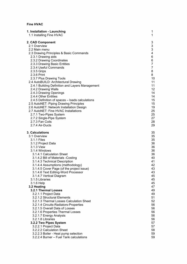
Fine HVAC 1. Installation - Launching 1

1.1 Installing Fine HVAC 1 2. CAD Component 3

2.1 Overview 3 2.2 Main menu 3 2.3 Drawing Principles & Basic Commands 4

2.3.1 Drawing aids 6 2.3.2 Drawing Coordinates 6 2.3.3 Drawing Basic Entities 7 2.3.4 Useful Commands 7 2.3.5 Grips 8 2.3.6 Print 8 2.3.7 Plus Drawing Tools 10

2.4 AutoBUILD: Architectural Drawing 11 2.4.1 Building Definition and Layers Management 11 2.4.2 Drawing Walls 12 2.4.3 Drawing Openings 14 2.4.4 Other Entities 14 2.4.5 Definition of spaces – loads calculations 15

2.5 AutoNET: Piping Drawing Principles 15 2.6 AutoNET: Network Installation Design 19 2.7 AutoNET: Fine HVAC Installations 25

2.7.1 Two-Pipes System 25 2.7.2 Single-Pipe System 27 2.7.3 Fan Coils 28 2.7.4 Air-Ducts 29

3. Calculations 35

3.1 Overview 35 3.1.1 Files 35 3.1.2 Project Data 36 3.1.3 View 36 3.1.4 Windows 36

3.1.4.1 Calculation Sheet 36 3.1.4.2 Bill of Materials -Costing 40 3.1.4.3 Technical Description 41 3.1.4.4 Assumptions (methodology) 42 3.1.4.5 Cover Page (of the project issue) 43 3.1.4.6 Text Editing-Word Processor 43 3.1.4.7 Vertical Diagram 45

3.1.5 Libraries 45 3.1.6 Help 45

3.2 Heating 47 3.2.1 Thermal Losses 49

3.2.1.1 Project Data 49 3.2.1.2 Structural Elements 51 3.2.1.3 Thermal Losses Calculation Sheet 52 3.2.1.4 Circuits-Radiators-Properties 56 3.2.1.5 Overall Data of Losses 56 3.2.1.6 Properties Thermal Losses 56 3.2.1.7 Energy Analysis 56 3.2.1.8 Libraries 56

3.2.2 Two Pipes System 57 3.2.2.1 Project Data 57 3.2.2.2 Calculation Sheet 58 3.2.2.3 Boiler - Heat pump selection 59 3.2.2.4 Burner – Fuel Tank calculations 59

3.2.2.5 Circulator calculation 59 3.2.2.6 Expansion Tank and Chimney calculations 60 3.2.2.7 Network Drawing 60 3.2.2.8 Vertical Diagram 61 3.2.2.9 Sections Friction Drop 61 3.2.2.10 Network Checking 61 3.2.2.11 Hot Water Storage Tank Calculations 61 3.2.2.12 Libraries 61

3.2.3 Single Pipe System 63 3.2.3.1 Project Data 63 3.2.3.2 Calculation Sheet 64 3.2.3.3 Calculation of other equipment 65 3.2.3.4 Vertical Diagram 65 3.2.3.5 Network Checking 65 3.2.3.6 Libraries 66

3.2.4 Infloor Heating System 67 3.2.4.1 Project Data 67 3.2.4.2 Calculation Sheet 68 3.2.4.3 Calculation of other equipment 71 3.2.4.4 Vertical Diagram 71 3.2.4.5 Libraries 71

3.3 Air-Conditioning 73 3.3.1 Cooling Loads 75

3.3.1.1 Indoor design conditions 75 3.3.1.2 Building Parameters 75 3.3.1.3 Climatological Data 75 3.3.1.4 Months 75 3.3.1.5 Structural Elements 76 3.3.1.6 People 77 3.3.1.7 Equipment 78 3.3.1.8 Lighting loads 79 3.3.1.9 Calculation Sheet 80 3.3.1.10 Temperatures 83 3.3.1.11 Building Loads Summary 83 3.3.1.12 Building Loads Analysis 84 3.3.1.13 Systems Loads Analysis 84 3.3.1.14 Total Loads Diagram (Without Ventilation) 84 3.3.1.15 Total Loads Diagram (With Ventilation) 85 3.3.1.16 Systems Diagram 85 3.3.1.17 Libraries 85

3.3.2 Fan Coils 87 3.3.2.1 Project Data 87 3.3.2.2 Calculation Sheet 88 3.3.2.3 Cooling Engine 89 3.3.2.4 Libraries 89

3.3.3 Air-Ducts 91 3.3.3.1 Project Data 91 3.3.3.2 Calculation Sheet 92 3.3.3.3 Fan Calculation 94 3.3.3.4 Libraries 95

3.3.4 Psychrometrics 97 3.3.4.1 Project Data 97 3.3.4.2 Psychrometric Point Calculations 99 3.3.4.3 Systems 100 3.3.4.4 Space Conditions – Cooling 105 3.3.4.5 Space Conditions – Heating 106 3.3.4.6 Systems Conditions – Cooling 106 3.3.4.7 Systems Conditions – Heating 106 3.3.4.8 Air-conditioning units 106

3.4 Examples 107 3.4.1. Building design example 107 3.4.2. Heating Network design example 113 3.4.3. Cooling Network design example 119

1. Installation - Launching

1.1 Installing Fine HVAC 1. Insert the CD in your computer CD-ROM drive (e.g. D:, E:) or, if you received your

software via Internet, run the installation application you downloaded.

2. When the Setup window appears, choose the language for the installation and click OK.

3. When the Welcome page appears (as shown below), click Next.

4. When the License Agreement appears, read it carefully. If you agree with the terms, check the respective “radio button” and then click Next (you must agree with the terms to proceed with the installation).

5. In the next screen enter your username and organization information and check if you want to create a desktop icon. Then click Next to see if the information is correct (see the following window) and finally click Install for the installation procedure to begin.

6. Upon completion of the installation procedure, the following last window appears on screen and all needed is to click Finish. In case that the Run Fine HVAC checkbox is selected, the program will start running.

FINE – HVAC - 1-

- 2 - FINE - HVAC

7. After installation, the program is located within the programs list.

2. CAD Component

2.1 Overview Fine HVAC is a powerful Workstation for Heating, Ventilation and Air-Conditioning Design, which automatically performs the necessary calculations directly from the drawings, producing all the case study results (calculation issue, technical descriptions, full-scale drawings, bills of materials etc.). This first Part (Part I) of the user's guide describes the operation of the CAD component of Fine HVAC. As mentioned in the preface, the CAD component is based on 4MCAD technology. Furthermore this CAD component is considering the building and HVAC installation as being composed of intelligent entities with their own attributes and properly related each one to each other. Fine HVAC CAD Component includes 2 main modules, which co-operate closely and give the Designer the impression he virtually works on the building: It is about a) AutoBLD that is used to load-identify the building and b) AutoNET that is used to design and identify the network installations. Those two subsystems are supported by a third one, with the name PLUS, which includes many useful designing facilities.

2.2 Main menu As soon as the program is loaded, the main menu screen appears for the first time:

Among the commands of the designing environment, we notice the following main options of the package:

1. Project files management options (New Project, Open Project and Project Information) which are located into the options group FILE.

FINE – HVAC - 3-

2. Option Group with the name AutoBLD, which includes all the commands required for the Architectural designing.

3. Option group with the name AutoNET, which includes all the commands required for the designing and calculation of the application (Single-pipe system, Two-pipe System, Air-ducts etc.).

4. Auxiliary option group with the name PLUS, which contains a series of designing facilities for the user.

Starting with FINE, you define a new project through the corresponding option in the FILE menu mentioned above. In case that "New project" is selected, a window appears on the screen where the name of the Project should be typed.

In order to "load" an existing project, which has been created with the program and you want to further edit it or just view it, you select "Select Project", and a list with the existing projects in the hard drive will be displayed on the screen. At first, the list displays all the projects that exist in the FINE directory and with the use of the mouse or the keyboard and acting correspondingly, you can transfer to any other directory, viewing at the same time the existing projects. It is noted that the projects are included into directories with the extension BLD. If an existing project is selected, it is loaded and displayed on the screen.

Either if a new project is created or a saved one is loaded, you can start working with the use of the subsystem commands described above. A detailed description of these commands is available in the following chapters. Before this detailed description, a short reference of the basic designing principles featured in the designing environment of the package is recommended, in chapter 2.3 that follows next. If you are familiar with the use of 4MCAD or AutoCAD, you may page through or even skip this chapter, while if you are not, you should read it carefully.

2.3 Drawing Principles & Basic Commands A great advantage of the package is that the structure and the features of the drawing environment follow the standards of the CAD industry adopted by AutoCAD, 4MCAD etc. In particular, the available working space is as follows:

- 4 - FINE - HVAC

As shown in the above figure, the screen is divided into the following "areas":

Command line: The command line is the area where commands are entered and the command messages appear.

Graphics area: The largest area of the screen, where drawings are created and edited.

Cursor: The cursor is used for drawing, selecting objects and running commands from the menus or the dialog boxes. Depending on the current command or action, the cursor may appear as a graphics cursor (crosshairs), a selection box, a graphics cursor with a selection box etc.

Pull-down menus: Each time you select one of these commands (AutoBLD, AutoNET etc.) a pull-down menu is shown.

Status Line: It is the line on the bottom of the screen where the current level, the drawing status and the current cursor coordinates are displayed. From the status line you can enable or disable tools such as SNAP, GRID, ORTHO etc., which are explained in the following chapter.

Toolbars: You can arrange which toolbars you want to be shown in the screen in each project. To enable or disable a toolbar, in the upper part of the screen (where the existing toolbars are shown) right click with the mouse and select the desired toolbar from the list (as it is shown below).

FINE – HVAC - 5-

Apart from that, each time you select an application from the AutoNET menu, a toolbar with the name of the application is shown and you can either work from there or from the AutoNET commands.

2.3.1 Drawing aids This section describes the most important drawing aids. These are the commands:

SNAP: The graphics cursor position coordinates appear in the middle of the upper part of the graphics area. If "Snap" is selected, the graphics cursor movement may not be continuous but follow a specific increment (minimum movement distance). To change the increment, right click with the mouse on “SNAP” and choose “Settings”. To activate or deactivate it, double click on the “SNAP” icon.

GRID: The screen grid is a pattern of vertical and horizontal dots, which are placed at the axes intersection points of an imaginary grid. The grid can be activated or deactivated by clicking the corresponding icon or by pressing F7.

ORTHO: The "Ortho" feature restricts the cursor to horizontal or vertical movement. The status bar shows whether the "Ortho" command is activated by displaying "ORTHO" in black characters. The command is activated or deactivated by clicking the corresponding icon or by pressing F8.

ESNAP: The "Esnap" command forces the cursor to select a snap point of an object, which is within the Pick box outline. The esnap points are characteristic geometric points of an object (i.e. endpoint of a line). If you have specified a snap point and move the cursor close to it, the program will identify it with a frame. The "Esnap" command can be activated either by holding down the "SHIFT" key and right clicking the mouse or through the additional toolbar.

2.3.2 Drawing Coordinates When you need to determine a point, you can either use the mouse (by seeing the coordinates in the status bar or using the snap utilities), or enter the coordinates directly in the command line. Moreover, you can use either Cartesian or polar coordinates and absolute or relative values, in each method (relative coordinates are usually more convenient).

Relative coordinates: Enter the @ symbol (which indicates relative coordinates) and then the x, y, z coordinates (Cartesian system) or the r<θ<φ coordinates (polar system) in the command line. The system used (Cartesian or polar) is defined by the “,” or “<” symbol respectively. If you do not insert a value for z or φ, it will be automatically taken as zero. For example, if you are prompted to locate the second (right) endpoint of a 2m horizontal line, you enter:

@2,0 if you use the Cartesian coordinates (which means that the distance of the second point from the first is 2 m on the x axis and 0 m on the y axis), or

@2<0 if you use the polar coordinates [which means that the second point is at a distance of 2m (r=2) and an angle of 0 degrees (θ=0) from the first].

Absolute coordinates: They are specified in the same way as the relative coordinates but without using the @ symbol. The absolute coordinates are specified in relation to the 0,0 point of the drawing.

The measurement system can be activated, deactivated or changed with the F6 key.

- 6 - FINE - HVAC

2.3.3 Drawing Basic Entities In the “Draw” menu you will find the basic drawing entities:

Line: "Line" option is used for drawing segments. When you select "Line" from the menu or type "Line" in the command line, you will be prompted to specify a start point (by left clicking or by entering the point coordinates – relative or absolute – in the command line) and an endpoint (determined in the same way).

Arc: The "Arc" command is used for drawing arcs. An arc can be drawn in different ways: the default method is to specify three points of the arc ("3-Points"). Alternatively, you can specify the start point and endpoint of the arc as well as the center of the circle where it belongs (St, C, End). You will not find it difficult to understand and become familiar with the various methods of drawing an arc.

Polyline: This command allows you to draw polylines, which are connected sequences of line or arc segments created as single objects. The command is executed by either using the menu or typing "pline" in the command line. You will be prompted to specify a start point and an endpoint (by right clicking the mouse or by entering the point coordinates – relative or absolute – in the command line). Then, the command options will appear (Arc, Close, Length etc). Select A to switch to Arc mode, L to return to Line mode and C to close the polyline.

2.3.4 Useful Commands This section includes brief descriptions of the basic program commands, which will be very useful. These are the commands "Zoom", "Pan", "Select", "Move", "Copy" and "Erase" (you will find them in “View” and “Modify” menus). In particular:

Zoom: "Zoom" increases or decreases the apparent size of the image displayed, allowing you to have a "closer" or "further" view of the drawing. There are different zooming methods, the most functional of which is the real-time zooming ("lens / ±" button). You can use the mouse to zoom in real time – that is to zoom in and out by moving the cursor. There are a number of zoom options as shown by typing "Zoom" in the command line: All/Center/Dynamic/Extents/Left/Previous/Vmax/window/<Scale(X/XP)>.

Pan: "Pan" ("hand" icon) moves the position of the visible part of the drawing, so that you can view a new (previously not visible) part. The visible part of the screen moves towards the desired area and to the desired extent.

Select: This command selects one or more objects (or the whole drawing), in order to execute a specific task (erase, copy etc.). Select is also used by other CAD commands (for example, if you use the "Erase" command, "Select" will be automatically activated in order to select the area that will be erased).

Move: This command allows moving of objects from one location to another. When the "Move" command is activated, the "Select" command is also activated so that the object(s) you want to move (in the way described in the previous paragraph) can be selected.

After you have selected the desired object(s), you are prompted to specify the base point (using the snap options), which is a fixed point of the drawing. When you are prompted to specify the position where the base point will be moved, use either the mouse or the snap options. After you have completed this procedure, the selected object(s) will move to the new position. Please note that the base and the new location points can be also specified with the use of coordinates (absolute or relative, see related paragraph).

Copy: The "Copy" option allows the copying of objects from one location to another. The "Copy" procedure is similar to the "Move" procedure and the only difference is that the copied object remains at its original location in the drawing.

FINE – HVAC - 7-

Erase: Choose this option to delete objects. The procedure is simple: Select the objects you wish to erase (as described above), type "E" in the command line and press <Enter>. Alternatively, you may first type "E" in the command line, then select the object(s) by left clicking and finally right click to erase the object(s).

DDInsert (Insert Drawing): This command allows you to insert another drawing (DWG file) or block in the drawing. When this command is selected, a window appears in which you select block or file and then select the corresponding block or file from disk. Then you are prompted to specify the insertion point, the scale factor etc., so that the selected drawing is properly inserted.

Wblock: The "Wblock" command allows us to save part of a drawing or the entire drawing in a file, as a block. When this command is selected, you are prompted to enter the file name and then you select the drawing or the part of the drawing you wish to save. The use of this command is similar to the "Screen Drawing" command in the AutoBLD menu, which will be described in a following section. In order to insert a block in a drawing, you use the "ddinsert" command described above.

Explode: The "Explode" command converts a block in a number of simple lines so that you can edit it in that form. If it is selected, the program will prompt you to select the block ("Select object") you wish to explode.

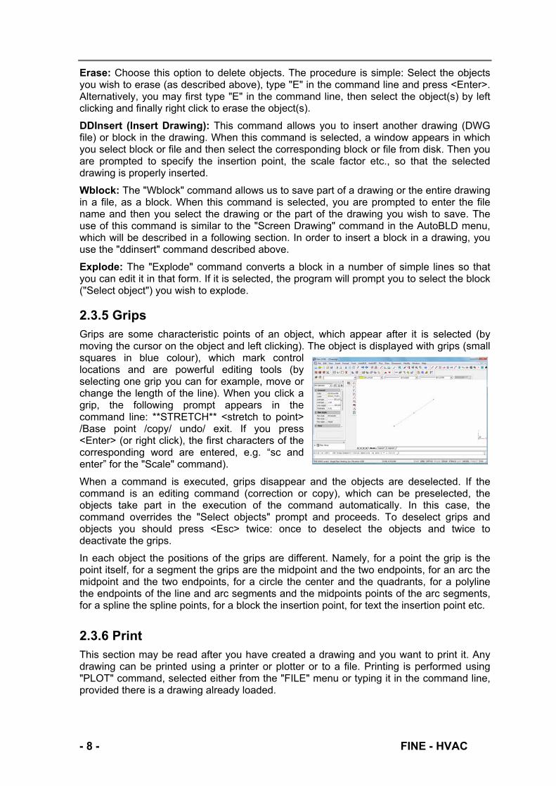
2.3.5 Grips Grips are some characteristic points of an object, which appear after it is selected (by moving the cursor on the object and left clicking). The object is displayed with grips (small squares in blue colour), which mark control locations and are powerful editing tools (by selecting one grip you can for example, move or change the length of the line). When you click a grip, the following prompt appears in the command line: **STRETCH** <stretch to point> /Base point /copy/ undo/ exit. If you press <Enter> (or right click), the first characters of the corresponding word are entered, e.g. “sc and enter” for the "Scale" command).

When a command is executed, grips disappear and the objects are deselected. If the command is an editing command (correction or copy), which can be preselected, the objects take part in the execution of the command automatically. In this case, the command overrides the "Select objects" prompt and proceeds. To deselect grips and objects you should press <Esc> twice: once to deselect the objects and twice to deactivate the grips.

In each object the positions of the grips are different. Namely, for a point the grip is the point itself, for a segment the grips are the midpoint and the two endpoints, for an arc the midpoint and the two endpoints, for a circle the center and the quadrants, for a polyline the endpoints of the line and arc segments and the midpoints points of the arc segments, for a spline the spline points, for a block the insertion point, for text the insertion point etc.

2.3.6 Print This section may be read after you have created a drawing and you want to print it. Any drawing can be printed using a printer or plotter or to a file. Printing is performed using "PLOT" command, selected either from the "FILE" menu or typing it in the command line, provided there is a drawing already loaded.

- 8 - FINE - HVAC

Viewing a drawing before printing gives you a preview of what your drawing will look like when it is printed. This helps you see if there are any changes you want to make before actually printing the drawing.

If you are using print style tables, the preview shows how your drawing will print with the assigned print styles. For example, the preview may display different colours or line weights than those used in the drawing because of assigned print styles.

To preview a drawing before printing

1. If necessary, click the desired Layout tab or the Model tab.

2. Do one of the following:

Choose File > Plot Preview.

On the Standard toolbar, click the Plot Preview tool .

Type ppreview and then press Enter.

3. After checking the preview image, do one of the following:

To print the drawing, click Plot to display the Print dialog box.

To return to the drawing, click Close.

The Plot dialog box is organized in several areas as it is shown in the picture below. For help defining print settings before you print, see Customizing print options.

In the plot window, you can select the printer, the paper size and the number of copies and several plot options such as the style (pen assignments), the orientation etc.

Moreover, you can select the plot scale and the plot area. Before you proceed to printing, you select “Apply to layout” and then “Preview” so as to make any modifications you might want.

To print a drawing

1. If necessary, click the desired Layout tab or the Model tab.

2. Do one of the following:

Choose File > Plot.

On the Standard toolbar, click the Print tool ( ). If you click the Print tool, the Print dialog box does not display. Your drawing will be sent directly to the selected printer.

Type print and then press Enter.

3. From the Plot dialog box, make any adjustments to the settings.

4. Click OK.

FINE – HVAC - 9-

2.3.7 Plus Drawing Tools Those tools belong to the large group of options under the general menu PLUS. These are a series of additional drawing tools, which have been embodied in the package in order to help the user during drawing.

- 10 - FINE - HVAC

2.4 AutoBUILD: Architectural Drawing The AutoBLD option group, as we will see in detail below, includes all the facilities required to insert a building in order to create an Architectural drawing. As it is shown in the corresponding AutoBLD menu, the various options are divided into sub-groups.

In general, the first sub-group includes commands for the definition of the project parameters, the second and the third sub-group includes drawing commands, the fourth sub-group includes commands for linking to the calculations, and the fifth sub-group includes management options for the AutoBLD libraries and commands for the building supervision. In the following sections, the options reported above are described one by one, starting from the "Building Definition" option.

2.4.1 Building Definition and Layers Management As soon as you select the "Building Definition" command, the levels management menu appears.

On this screen the levels of the project building are defined, which means that you have to determine the level and the corresponding architectural drawing (plan view-as xref) (DWG file) of each building floor (only in case you use a drawing that was created by another architectural designing program). More specifically:

In the "Level" field, define the level (floor) number (always starting with the number “1”).

FINE – HVAC - 11-

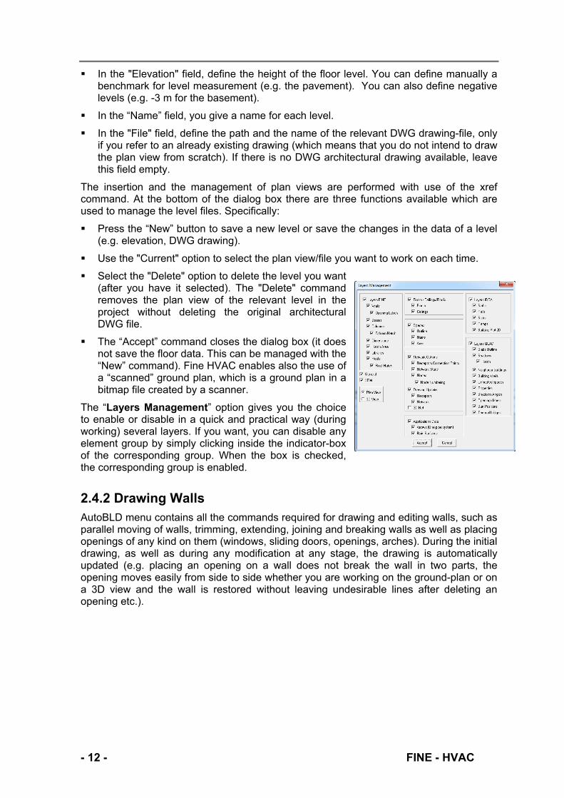
In the "Elevation" field, define the height of the floor level. You can define manually a benchmark for level measurement (e.g. the pavement). You can also define negative levels (e.g. -3 m for the basement).

In the “Name” field, you give a name for each level.

In the "File" field, define the path and the name of the relevant DWG drawing-file, only if you refer to an already existing drawing (which means that you do not intend to draw the plan view from scratch). If there is no DWG architectural drawing available, leave this field empty.

The insertion and the management of plan views are performed with use of the xref command. At the bottom of the dialog box there are three functions available which are used to manage the level files. Specifically:

Press the “New” button to save a new level or save the changes in the data of a level (e.g. elevation, DWG drawing).

Use the "Current" option to select the plan view/file you want to work on each time.

Select the "Delete" option to delete the level you want (after you have it selected). The "Delete" command removes the plan view of the relevant level in the project without deleting the original architectural DWG file.

The “Accept” command closes the dialog box (it does not save the floor data. This can be managed with the “New” command). Fine HVAC enables also the use of a “scanned” ground plan, which is a ground plan in a bitmap file created by a scanner.

The “Layers Management” option gives you the choice to enable or disable in a quick and practical way (during working) several layers. If you want, you can disable any element group by simply clicking inside the indicator-box of the corresponding group. When the box is checked, the corresponding group is enabled.

2.4.2 Drawing Walls AutoBLD menu contains all the commands required for drawing and editing walls, such as parallel moving of walls, trimming, extending, joining and breaking walls as well as placing openings of any kind on them (windows, sliding doors, openings, arches). During the initial drawing, as well as during any modification at any stage, the drawing is automatically updated (e.g. placing an opening on a wall does not break the wall in two parts, the opening moves easily from side to side whether you are working on the ground-plan or on a 3D view and the wall is restored without leaving undesirable lines after deleting an opening etc.).

- 12 - FINE - HVAC

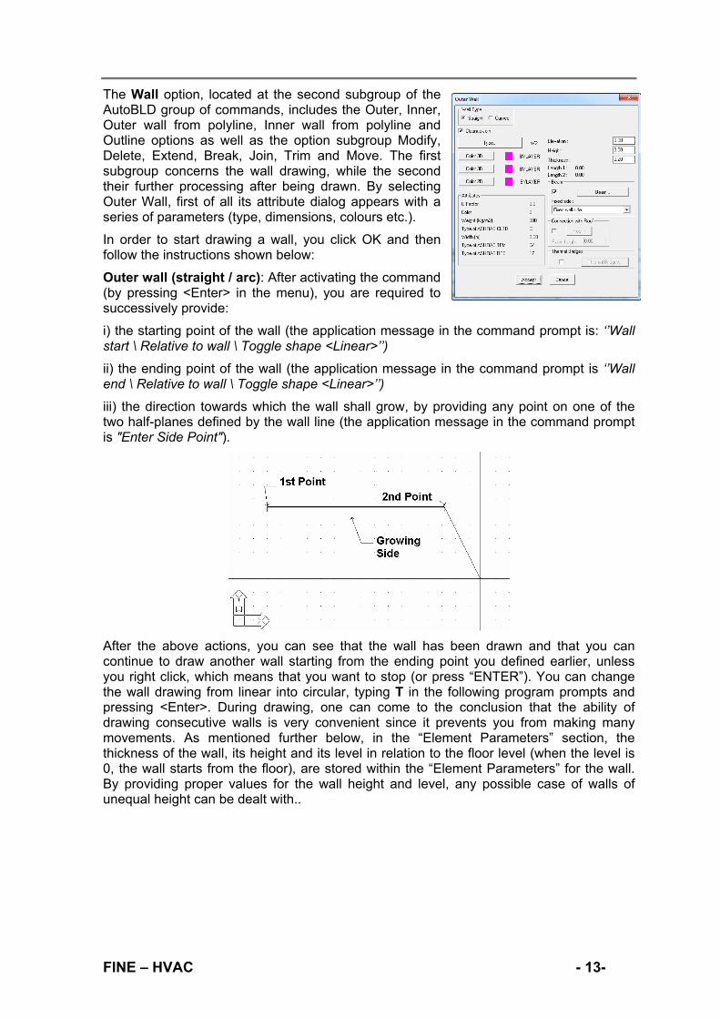
The Wall option, located at the second subgroup of the AutoBLD group of commands, includes the Outer, Inner, Outer wall from polyline, Inner wall from polyline and Outline options as well as the option subgroup Modify, Delete, Extend, Break, Join, Trim and Move. The first subgroup concerns the wall drawing, while the second their further processing after being drawn. By selecting Outer Wall, first of all its attribute dialog appears with a series of parameters (type, dimensions, colours etc.).

In order to start drawing a wall, you click OK and then follow the instructions shown below:

Outer wall (straight / arc): After activating the command (by pressing <Enter> in the menu), you are required to successively provide:

i) the starting point of the wall (the application message in the command prompt is: ‘’Wall start \ Relative to wall \ Toggle shape <Linear>’’)

ii) the ending point of the wall (the application message in the command prompt is ‘’Wall end \ Relative to wall \ Toggle shape <Linear>’’)

iii) the direction towards which the wall shall grow, by providing any point on one of the two half-planes defined by the wall line (the application message in the command prompt is "Enter Side Point").

After the above actions, you can see that the wall has been drawn and that you can continue to draw another wall starting from the ending point you defined earlier, unless you right click, which means that you want to stop (or press “ENTER”). You can change the wall drawing from linear into circular, typing T in the following program prompts and pressing <Enter>. During drawing, one can come to the conclusion that the ability of drawing consecutive walls is very convenient since it prevents you from making many movements. As mentioned further below, in the “Element Parameters” section, the thickness of the wall, its height and its level in relation to the floor level (when the level is 0, the wall starts from the floor), are stored within the “Element Parameters” for the wall. By providing proper values for the wall height and level, any possible case of walls of unequal height can be dealt with..

FINE – HVAC - 13-

Further to the drawing functions, the program also provides powerful editing tools, such as erase, modify (through the wall dialog box), multiple change etc. Two other commands that are widely used while drawing the walls are a) the Undo command, which enables you to reverse the previous command executed and b) the Properties command, which enables you to view (and change) the attributes of the selected wall.

2.4.3 Drawing Openings Once the command "Opening" is activated, a second option menu is displayed, including a variety of opening types (window, sliding door, door etc) to draw, plus also a set of editing functions such as "Erase", "Modify" or "Move", applied to existing openings. Besides, at the bottom of this menu lies the option “Libraries”, which enables the user to define his/her own opening freely, to create various shapes of windows.

Window: The option "Window" demands that you select the wall on which the opening will be placed and then define the beginning and the end of the opening (all these actions are carried out using the mouse and pressing <Enter> each time). The window will automatically obtain the data that are predefined in the “Attributes”, namely the corresponding values for the height, the rise, the coefficient k etc). Of course, you can draw the window from the ground plan as well as in the three-dimensional (3D) view. During drawing a window, it is very helpful to the user the fact that, after the wall where the window will be automatically placed is selected, the distance from the wall edge is displayed in the coordinates position on the top of the screen, while the crosshair is transferred parallel to the wall for supervision reasons. The measurement starting point (distance 0) as well as the side (internal or external) are defined by which one of the two edges is closer and which side was "grabbed" during the wall selection. Similar functionality exists for other types of openings, such as Sliding Doors, Doors, Openings etc.

2.4.4 Other Entities AutoBLD provides tools for designing columns and other elements, as well as drawing libraries including drawings and symbols to place within the drawing (i.e. general symbols, furniture, plants etc.).

Finally, the Building model of a Fine HVAC project can be viewed through the commands:

Plan View (2D): The two-dimensional plan view of the respective building level is shown.

3D View: A three-dimensional supervision of the ground plan of the current floor (with given viewing angles) is shown.

- 14 - FINE - HVAC

Axonometric: Provides three-dimensional supervision of the whole building (for all floors), with the given viewing angles as they have been selected in "Viewing Features".

2.4.5 Definition of spaces – loads calculations The Fine HVAC building model includes intelligent information, capable to recognise the spaces and their heating and cooling loads. More specifically, the “space definition” command enables the user to define one or more spaces, in two alternative ways

a) by selecting the walls that surround each space, or

b) by defining an internal and an external point of the space. This way needs only the definition of an internal point of the space (by a left click of the mouse) and an external point so that the line-rubber that is formed intersects a space wall. Then the program "indicates" (by discontinuous outline) the defined space and asks for the space name in the command line. By entering the name the space definition is completed and its features are indicated on the drawing. Given that one or more spaces are already defined, the command "Calculations" serves to calculate the Thermal losses and Cooling loads of the building. Each one of the commands “Thermal losses” or “Cooling loads” activates the respective application window. In each window, first of all, you have to select the “Update from drawing” command (located at the “Files” menu) in order to transfer the drawing data automatically (see paragraphs 3.2.1 and 3.3.1).

2.5 AutoNET: Piping Drawing Principles The AutoNET group includes all those tools the designer needs in order to draw (and then calculate) the HVAC piping installations. Below are described the general AutoNET commands and you will find the specific commands for FINE HVAC applications in the next chapters.

Drawing Definition: The layers for each installation are organised properly and the information is shown on the respective dialog. The command "Colour" is used to assign the desired colour to each network while the command "Linetype" is used to select the desired line type.

Applications Layers Management: This command leads to a dialog screen where you can activate more than one applications and monitor those which are possibly overlapping (i.e. both Single pipe and Fan coils networks at the same time).

Copy network of Level: ΑutoNET enables copying of typical (installation) plan views and pasting them on other levels through this command, which functions similarly to the “copy level” AutoBLD option. When you select this command, the program prompts you to select the network you want to copy (you can select it in a window), and after you do it and press ENTER, it asks you to give the number of the level in which you want to copy it.

Select Application: This option enables selection of the desired application of Fine HVAC. Depending on the selected application, the section of the following AutoNET menu will be configured accordingly.

The basic principles and rules for drawing a network are described below:

Network Drawing: The installation network drawing is carried out with a single line, by drawing lines and connecting them to each other, exactly as the network is connected in fact. You should keep in mind some general principles regarding drawing and connecting between straight or curved, horizontal or vertical network branches.

FINE – HVAC - 15-

Horizontal & Vertical Piping: In any case, the piping drawing is carried out exactly as the line drawing (in AutoCAD or 4MCAD). You are able to draw horizontal or vertical pipes. The pipe installation elevation is the current elevation. Modification of the pipe installation elevation is possible through the menu PLUS -> Set elevation (or if you type the command "elev"). If you type "elev" (in the command line), you are prompted to determine the new current elevation. Press <Enter> if it is 0 or type the value you want. At this point it should be emphasised that, if a horizontal piping which is found on a specific level is drawn and it is connected to another piping or a contact point (receptor), the program automatically "elevates" or "lowers" the pipe so that connecting to the other pipe or receptor, respectively, is possible. In this way, the program facilitates the drawing of piping in three dimensions while you are actually working in a two-dimension environment. In any case of a network design, all facilities provided by AutoCAD can be utilised through relative co-ordinates.

Vertical pipe Drawing: Drawing vertical pipes which cross floors (one or more) is possible through the option "Main Vertical pipes (Building)". When the respective option is selected from the menu, the program asks for the pipe position ("Enter xy Location") and then for the height of the starting point ("Enter Height for First Point") as well as the height of the ending point ("Enter Height for Second Point"). For example, if you want to draw a vertical pipe from 0 to 3, by inserting the location point (XY) and then the numbers 0 and 3 successively, the symbol for direction change appears on the ground plan and in 3D View.

Vertical sections within the same floor: If you want to elevate or lower a pipe within the same floor, you can use the relative coordinates. For example, if you have drawn a horizontal pipe (in elevation of 0 m) and you want to elevate it to 2 m, when in the command line asks for “Enter next point”, you will type @0,0,2 and continue drawing the pipe (see the adjacent photo). In the same way, if you want to lower the pipe by 2 m, you will type @0,0,-2.

Drawing of Curved Pipes: You can draw curved pipes by inserting the points from which the curved pipe is to pass (give at least 3 points). The respective command prompts for the following:

First point: Insert the starting point of the pipe.

Next point: Insert next point, the one after that and so on (successively), defining the pipe routing in this way and to stop press <ENTER> or right click of the mouse.

- 16 - FINE - HVAC

The user can easily modify curved pipes using “grips". As soon as the pipe is selected, grips appear which you can move, altering this way the pipe routing. In the Bill of Materials and the Calculations phase, the program will measure the pipe length precisely.

Connecting network sections: Connections between network sections (horizontal, vertical or both) as well as between network parts and receptors can be easily executed by using the "Snap" commands. For example, suppose that the two horizontal parts of the ground plan below, which are placed in different heights, have to be connected. If you start by "grabbing" the "upper" pipe end and then end up at the "lower" pipe end, the result in the three-dimension representation will be as on the right.

Another example, the result of the connection of a radiator starting from its "connection point" and ending at the base point of the vertical pipe is shown below. Alternatively, you can use the “Connect radiators to an existing pipe” command where after you define the pipe and the radiators you want to be connected to it, the program connects them automatically.

FINE – HVAC - 17-

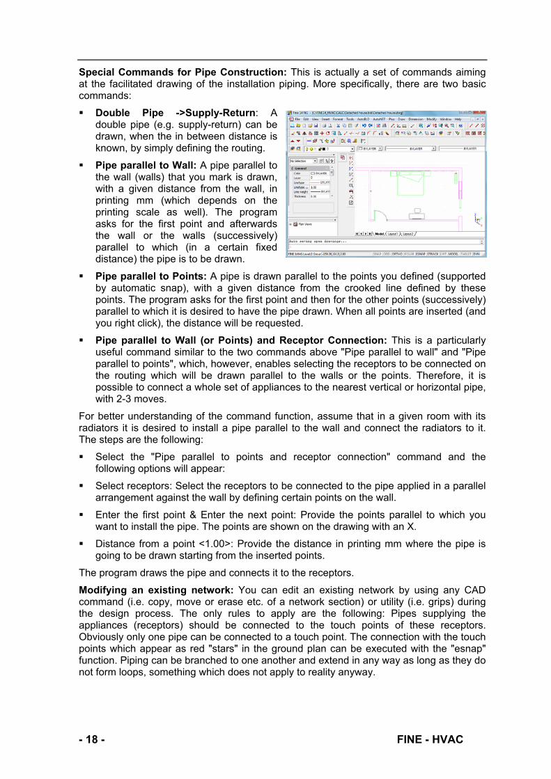
Special Commands for Pipe Construction: This is actually a set of commands aiming at the facilitated drawing of the installation piping. More specifically, there are two basic commands:

Double Pipe ->Supply-Return: A double pipe (e.g. supply-return) can be drawn, when the in between distance is known, by simply defining the routing.

Pipe parallel to Wall: A pipe parallel to the wall (walls) that you mark is drawn, with a given distance from the wall, in printing mm (which depends on the printing scale as well). The program asks for the first point and afterwards the wall or the walls (successively) parallel to which (in a certain fixed distance) the pipe is to be drawn.

Pipe parallel to Points: A pipe is drawn parallel to the points you defined (supported by automatic snap), with a given distance from the crooked line defined by these points. The program asks for the first point and then for the other points (successively) parallel to which it is desired to have the pipe drawn. When all points are inserted (and you right click), the distance will be requested.

Pipe parallel to Wall (or Points) and Receptor Connection: This is a particularly useful command similar to the two commands above "Pipe parallel to wall" and "Pipe parallel to points", which, however, enables selecting the receptors to be connected on the routing which will be drawn parallel to the walls or the points. Therefore, it is possible to connect a whole set of appliances to the nearest vertical or horizontal pipe, with 2-3 moves.

For better understanding of the command function, assume that in a given room with its radiators it is desired to install a pipe parallel to the wall and connect the radiators to it. The steps are the following:

Select the "Pipe parallel to points and receptor connection" command and the following options will appear:

Select receptors: Select the receptors to be connected to the pipe applied in a parallel arrangement against the wall by defining certain points on the wall.

Enter the first point & Enter the next point: Provide the points parallel to which you want to install the pipe. The points are shown on the drawing with an X.

Distance from a point <1.00>: Provide the distance in printing mm where the pipe is going to be drawn starting from the inserted points.

The program draws the pipe and connects it to the receptors.

Modifying an existing network: You can edit an existing network by using any CAD command (i.e. copy, move or erase etc. of a network section) or utility (i.e. grips) during the design process. The only rules to apply are the following: Pipes supplying the appliances (receptors) should be connected to the touch points of these receptors. Obviously only one pipe can be connected to a touch point. The connection with the touch points which appear as red "stars" in the ground plan can be executed with the "esnap" function. Piping can be branched to one another and extend in any way as long as they do not form loops, something which does not apply to reality anyway.

- 18 - FINE - HVAC

If however a mistake occurs, the program (during the recognition procedure) will perform all checks and indicate the mistake and its location. A necessary step before the "Network recognition” is defining the point (1) where the network starts, that is the supply point (1). In reality, this point corresponds to the Fire Pump. In Fine HVAC application, the menu includes the specific options, so that you can be easily guided when drawing any installation.

2.6 AutoNET: Network Installation Design The previous chapter described the drawing principles, while the present one describes those commands in relation to the special features of Fine HVAC.

Regardless of the fact if there is an AutoBLD building model, an external reference, a digital image or even no architectural drawings, a Fine HVAC installation can be drawn and then calculated.

Although there are no limitations regarding the order of actions followed in drawing an installation, the following order is suggested:

Place the receptors (Radiators, Grilles etc.)

Draw the horizontal pipes (or air ducts)

Connect the receptors to the pipes

Draw the vertical pipes

Connect the horizontal to the vertical pipes

Define the Supply point(s)

Run “Network Recognition”

If there are no mistake messages, proceed to the calculations

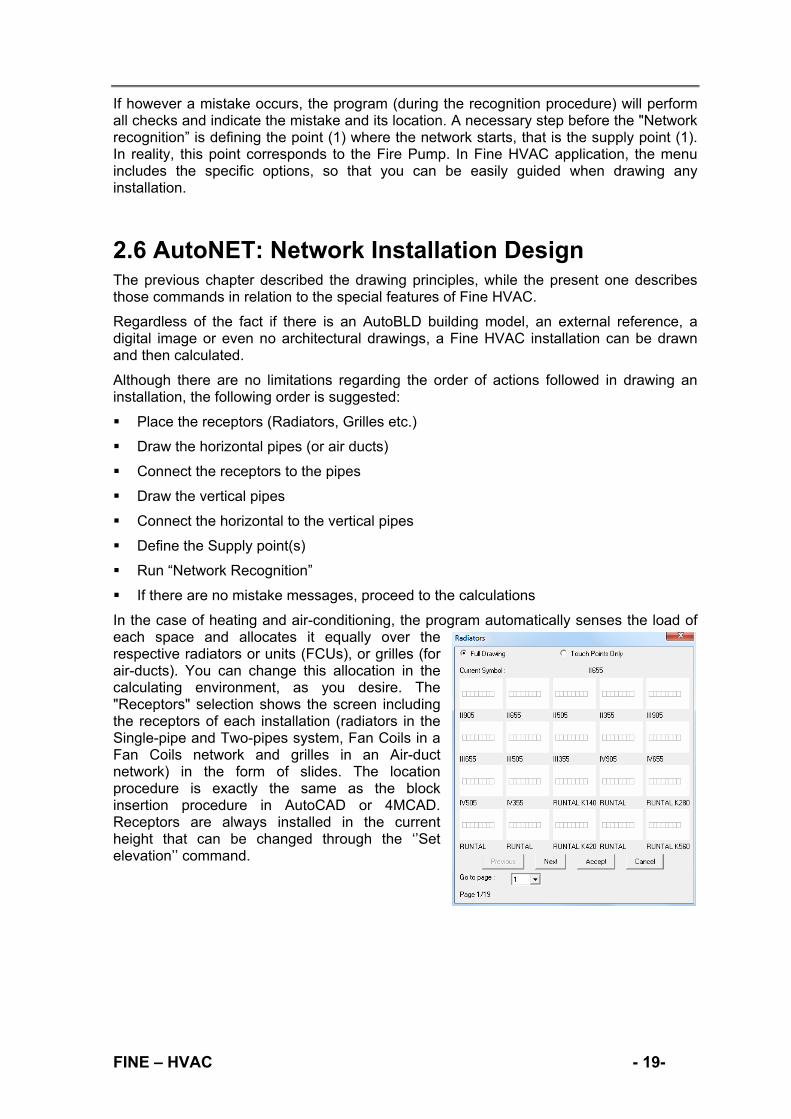
In the case of heating and air-conditioning, the program automatically senses the load of each space and allocates it equally over the respective radiators or units (FCUs), or grilles (for air-ducts). You can change this allocation in the calculating environment, as you desire. The "Receptors" selection shows the screen including the receptors of each installation (radiators in the Single-pipe and Two-pipes system, Fan Coils in a Fan Coils network and grilles in an Air-duct network) in the form of slides. The location procedure is exactly the same as the block insertion procedure in AutoCAD or 4MCAD. Receptors are always installed in the current height that can be changed through the ‘’Set elevation’’ command.

FINE – HVAC - 19-

Example: Suppose that a grille has to be installed in 2.85 m height from the floor. After selecting "Set elevation" (from the PLUS menu) or executing the "elev" command by typing it in the command line and inserting value 2.85, press <Enter> in the receptor screen "on" a grille and afterwards press "OK" (or alternatively double click). Then you can see the grille moving on the ground plan together with the graphic cursor.

If the mouse is moved properly the grille can be carried in such a way that its base point (which coincides with the cross of the graphic cursor) will be placed in the respective point.

It can now be observed that if the mouse is moved, the grille rotates around the base point. Thus, if you confirm the angle in which you desire to install the receptor, the grille can be seen in its final position.

- 20 - FINE - HVAC

It is possible not to install the whole receptor if it already exists in the architectural ground plan (if it has been drawn by the Architect), but activate the "Touch Points Only" indication in the upper side of the receptor selection window, so that only the receptor touch point will be selected in order to install it in the appropriate position.

“Receptors grid”, as well as the “Automatic radiators placement”, are two additional options.

Fittings: The "Fittings" command selects the accessories to be also inserted in the drawings, which applies exactly the same as the receptors. Fittings have "touch points" upon which the piping will be connected so that the network can be recognised. A symbol may also have more than one touch points (e.g. a collector), in which case the fitting will be numbered as a junction point in the "Network Recognition". The program provides the capability of cutting off the line automatically when a symbol is inserted on the line, exactly where the accessory interjects. This capability is defined by the indication of the accessories box "Break Pipe". If this option is activated, then the program will automatically "Break" the pipe when the accessory is placed. Moreover, the "Move Symbol" indication is in the same box, which defines whether the accessory will be moved in relation to the position it was initially placed (so that it will be placed parallel and on top of the pipe) or the pipe will be moved (so that the accessory can be attached).

Symbols: "Symbols" include various general symbols, layout of machines (i.e. pressure units) and other drawings that can be used in the corresponding installation.

FINE – HVAC - 21-

Network Recognition and Numbering: Since the network has been drawn according to the current rules and the supply point has been determined, the "Network Recognition" option converts the network in the required standard pattern and updates appropriately the calculation sheet. During updating, junction points and receptors are numbered on the ground plan. Note that if a receptor is not numbered, means that it is not connected to the network. Besides, if a network section has a different colour it cannot be connected to the network. Connect it or select "Break at selected point" at the connection point with the previous pipe.

Calculations: The "Calculations" option leads you in the corresponding calculating environment, which means that the window of the current application is “opening”, while FINE HVAC always remains "open". In order to transfer the data from the drawings, you select "Update from Drawing" in the menu "Files" of the corresponding calculating application (in order to carry out the corresponding calculations, answer "Yes" to the question "Calculate" that appears). It has to be noticed that the numbering of the sections, the lengths of the network sections, the receptors with their supplies and the fittings (from the piping routing) are transferred in the calculation sheet. Of course, if you want to, you can intervene in the calculations in order to make any modifications.

Update Drawing: After the calculation part of the program is completed, save the project file, return to the drawing program (FINE HVAC) and select “Update Drawing”. The following window will open and you will select the information you want to be shown on the drawing. Particularly:

- In the left part of the window, you select the information you want to be shown regarding the pipes (or air ducts). You can select to see information for all the pipes (choose “Select All”), some of them (choose “Select from Drawing” and select the pipes from the drawing) or none (choose “Deselect All”). Furthermore, below this list, you can choose which information you want to be shown, such as the length, the flow rate, the diameter etc. If you do not want, for example, the “Velocity” to be shown, select it and uncheck the “Selection” button.

- In the right part of the window, you select the information you want to be shown regarding the receptors. You can select to see information for all the receptors (choose “Select All”), some of them (choose “Select from Drawing” and select the receptors from the drawing) or none (choose “Deselect All”). Furthermore, below this list, you can choose which information you want to be shown, such as the receptor name, the water flow etc. If you do not want, for example, the “Group” to be shown, select it and uncheck the “Selection” button.

Finally, to place the information on the drawing, select either “Manually placement” or “Auto Placement” (the program automatically chooses to place the information for each pipe and receptor in the best position without covering each other).

- 22 - FINE - HVAC

Convert single line to 3D: After the drawing has been updated, you can convert the single lines to 3D pipes or air ducts (depending the application you are working on), by choosing this command. The dimension of the 3D pipes and air ducts will be related to the calculation results. When you select this command, in the command line you will have to define which network will be converted to 3D (supply, return or both) and in which level (one or all) and the drawing once again will be automatically updated.

Legend: The "Legend" option creates a legend with all the symbols that have been used in this specific project. By selecting it, the program asks for the location where the Legend is going to be inserted. Use the mouse to define the location and the legend will appear automatically on your screen, exactly under the location point.

Vertical Diagram: This option is used for the automatic creation of the vertical diagram of the installation and in its appearance on the screen, within few seconds. In case there is already a vertical diagram, the program asks if you want to update it. It is obvious that, in order to create a vertical diagram, you should draw and identify a network and enter the calculation sheet, so that the program knows all the data needed for the vertical diagram creation (pipe dimensions, junction points numbering, etc). By the “creation” command the window of the vertical diagrams manager appears on screen. This window is composed of two parts, the part with the network tree and the part with the vertical diagram. Through specific commands, the user can intervene in several ways on the output of the diagram:

Enable or disable various branches of the network

Change the order of the columns of sub-networks in the vertical diagram

FINE – HVAC - 23-

Change the sub-networks direction connection on the vertical columns (right or left)

Read the information of each node

Describe the sub-networks

The changes done in the vertical diagram are displayed in real time, in the second part of the window. On the upper side of this window there are also icons for processing the diagram (real time zoom and pan, zoom extends etc). In addition, in the upper-left side there are some other icons having to do with the appearance of the screen, such as the hiding of the left part of the window, the appearance of the level names and heights on the left to be edited, the appearance of the numbers of the receptors, the layers and others.

Finally there are some options for the initialization of the vertical diagram, its recreation and the definition of the drawing parameters. In particular, these parameters depend on the application and include the following options:

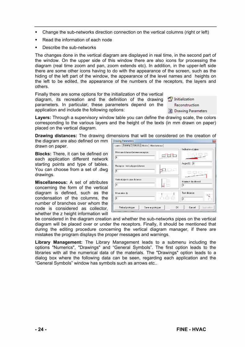
Layers: Through a supervisory window table you can define the drawing scale, the colors corresponding to the various layers and the height of the texts (in mm drawn on paper) placed on the vertical diagram.

Drawing distances: The drawing dimensions that will be considered on the creation of the diagram are also defined on mm drawn on paper.

Blocks: There, it can be defined on each application different network starting points and type of tables. You can choose from a set of .dwg drawings.

Miscellaneous: A set of attributes concerning the form of the vertical diagram is defined, such as the condensation of the columns, the number of branches over whom the node is considered as collector, whether the z height information will be considered in the diagram creation and whether the sub-networks pipes on the vertical diagram will be placed over or under the receptors. Finally, it should be mentioned that during the editing procedure concerning the vertical diagram manager, if there are mistakes the program displays the proper messages and warnings.

Library Management: The Library Management leads to a submenu including the options "Numerics", "Drawings" and “General Symbols”. The first option leads to the libraries with all the numerical data of the materials. The "Drawings" option leads to a dialog box where the following data can be seen, regarding each application and the “General Symbols” window has symbols such as arrows etc..

- 24 - FINE - HVAC

2.7 AutoNET: Fine HVAC Installations In this section AutoNET commands are described in relation to the special features of each application, which means that the general features are analysed and the special features applying to each installation network are pointed out.

2.7.1 Two-Pipes System The basic AutoNET drawing principles apply here as well. Generally, a typical two-pipe heating system network (parallel induction-return networks) is drawn according to the following procedure:

Install radiators on the ground plans

Radiators are installed on the ground plans either by running the "Radiators" command and selecting from the appearing dialog box the type which will be used (size will be estimated in the calculating environment) or by running the "Automatic radiators placement" command and selecting the spaces where automatic installation will take place (on the condition that spaces are defined on the ground plan and their thermal losses are calculated).

Draw horizontal supply and return pipes (simply or parallel to walls, points etc.) and connect them to the radiators (automatically or manually)

Draw vertical pipes

Install fittings such as collectors (optional)

Connect horizontal to vertical pipes (directly or through collectors)

Place network starting points

Run network recognition

Proceed to the calculations (pipe lengths and the respective fitting number will be automatically inserted in the calculation sheets)

Ground plan update including transfer of calculated types, radiator loads and pipe dimensions through the “Update drawing” command (see paragraph 2.6 for more information)

Convert single lines to 3D pipes (optional)

Create the Vertical Diagram

In two-pipes system you can design only the supply network and not the return and when you proceed to the calculations the program will automatically double the length of the network sections so as to calculate the return network as well.

In case that the supply is not parallel to the return network (or if they are parallel and the user wants to draw them), then two independent networks should be drawn (one for the supply and one for the return network) as well as two starting points in the network willl be placed (supply point and return point). After recognition, two networks will be transferred in the calculation sheet (supply with "." and return with "-" symbol) according to the valid standardisation required from the calculating environment (see Two-Pipes System calculating environment).

For example, in the following screen appears a section of a Two-Pipe installation, where we have drawn only the supply section, which however is enough for the analytical calculation of the installation:

FINE – HVAC - 25-

In the above example radiators are connected automatically to the columns through small horizontal sections.

You are absolutely free to draw horizontal and vertical sections as well as columns, according to the example in section 5.1. The network starting point is provided with the command “Supply Start Point” (Boiler), while a return point is required only if there is a return network.

Apart from the above general functions, you should also be aware of the following:

The space loads are distributed equally over the radiators installed within the space. From this point on, the user is able to interfere in the calculating environment in order to distribute the total load over the radiators, exactly as it is desired.

- 26 - FINE - HVAC

The program recognises as space load the modified (perhaps) space load which exists in the "Thermal Losses" and not the one which the program had initially “read" from the ground plan.

The program shows error messages in case that the network does not fulfil the logical drawing rules (i.e. there is a short circuit, a point where pipes of supply and return end up etc.), while the wrong connected sections are shown with a different colour.

2.7.2 Single-Pipe System The general AutoNET principles apply in the Single-Pipe System application as well. However, there are several variations which result from the fact that the standardisation applied in the Single-Pipe System application differs from the others significantly. In general, a Single-Pipe Heating System network is drawn following the order described below:

Install radiators on the ground plans (automatically or manually):

Radiators are installed on the ground plans either by running the "Radiators" command and selecting from the appearing dialog box the type which will be used (size will be estimated in the calculating environment) or by running the "Automatic radiators placement" command and selecting the spaces where automatic installation will take place (on the condition that spaces are defined on the ground plan and their thermal losses are calculated).

Draw the main vertical pipes (supply and return):

Define the location where the vertical pipes will be placed as well as their starting and ending points. Note that the vertical pipe heights should be provided in relation to the heights determined for the building floors.

Install collectors on the ground plans

Install the supply and return collectors which are found on the various building floors on the ground plan. Collector installation is carried out by running the "Fittings" command and selecting the respective desired collectors from the appearing dialog box. Keep in mind that the collector connection points are just drawing symbols, so you can connect more than one circuit pipes to each connection point.

Draw horizontal pipes from collectors to columns

Draw the network section connecting the supply collector to the supply vertical pipe as a supply horizontal pipe. Regarding the pipe drawing, first you select the point of the collector (you can use the "Set point snap" to help you) and then the vertical pipe (for the vertical pipe you can use the "Perpendicular snap" to help you). The vertical pipe is not represented by the arrow but by the dot displayed in the middle of it (this is the projection of the vertical pipe on the ground plan).

The same steps are followed for the connection of the return collector to the return vertical pipe.

Draw the circuits that connect the collectors to the radiators. You can either draw the circuits manually or automatically. If you want to draw them automatically, you select the “Automatic placement” command. You start from the supply collector and select the first radiator (you can then see the circuit section forming until the first radiator), continue to the second (you select it in the same way) and so on until the last radiator you want to be included in this circuit. When you finish, you press “ENTER” and select the return collector so as to close the circuit. Circuits can be drawn using either straight or curved pipes.

FINE – HVAC - 27-

Define the network start points (supply and return) of the installation

Place the supply and return points by using the option “Network Start Point” and selecting the endpoint of the respective pipe through “End Point” snap.

Network Recognition

If the command “Network Recognition” is activated, the program identifies the circuits as well as the radiator locations in the spaces and prepares linking files to the calculation sheets. If something hasn’t been drawn correctly, you will get a message which informs you where exactly is the problem.

Calculations

Select the option “Calculations” to call the calculation program of the Single-Pipe application, where data are transferred to the calculation sheet when the option "Update from Drawing", under "Files" menu, is selected.

Update Drawing

If this option is selected, the calculated radiator types and loads as well as the circuit data are transferred to the ground plan. If the ground plan has been updated before, the program prompts you to update the ground plan erasing the old data (see paragraph 2.6 for more information).

Insert arrows on circuits

Run the command “Circuit arrows placement” to insert arrows automatically on the circuits, following the direction from the supply collector to the return collector (you can find the command in AutoNET -> Network start point menu).

Convert single lines to 3D pipes (optional)

Create the Vertical Diagram

The vertical diagram is created according to the DXF file, generated by the calculation module.

2.7.3 Fan Coils Everything mentioned above about the Two-Pipe system, applies here as well. Besides, in order to transfer the calculated cooling loads, in the Cooling Loads program, the user has to choose from the "Files" menu the option Export to -> Fan coils. There he can also select whether he wants to transfer the "Total Loads" (e.g. in case only FCUs are used for cooling) or the "Space Loads" (e.g. in case there is a FCU and a central air-conditioning unit which precools the air induced in the space) or the "Ventilation Loads" (rare case). Otherwise, the user has to enter manually the load which corresponds to each FCU in the calculation sheet. Apparently, in the case of more than one FCU units, the space loads are distributed equally over the FCU units installed within the particular space. From this point on, you are able to interfere in the calculating environment in order to distribute the total load over the FCUs, exactly as it is desired.

Furthermore, you should also be aware of the following:

The space loads are distributed equally over the Fan Coils installed within the particular space. From this point on, you are able to interfere in the calculating environment in order to distribute the total load over the FCUs, exactly as it is desired.

The program recognises as space load the modified (perhaps) space load which exists in the "Cooling Losses" and not the one which the program had initially “read" from the ground plan.

- 28 - FINE - HVAC

The program shows error messages in case that the network does not fulfil the necessary rules.

2.7.4 Air-Ducts An air-duct network can be drawn in one dimension so that it can be identified and transferred to the calculation sheet automatically. Moreover, there is also the possibility to draw in two or three dimensions for detailed and complete air-duct ground plan drawings. These three possibilities can be used independently as well as in combination with each other. The greater interest lies within the automatic creation of a two-dimensional drawing starting from a linear (one-dimensional) one. First draw the linear (one-dimensional) figure, proceed to the network identification, carry out the calculations and update the ground plan with the calculation results (air-duct and grille dimensions). Then run the command "Convert single line into 2D" to receive the two-dimensional drawing of the air-ducts, completely automatically, on the basis of the calculation results. Moreover, you can use the “Convert single line to 3D” command so as to receive directly the three-dimensional drawing (after the calculations have been made).

More specifically, a linear air-duct network, either supply or return, is drawn according to the following procedure:

Install grilles on the ground plans (automatically or manually)

Draw vertical ducts

Draw horizontal ducts (connect them to grilles)

Define the network starting point (supply or return point)

Run Network Recognition

Proceed to the Calculations

Update the ground plans concerning transfer of the calculated dimensions

Convert single lines to 3D (optional)

Create the Vertical Diagram

The above procedure should be followed separately for the supply network as well as for the return network. During the design process, the program detects and shows all the possible error messages.

FINE – HVAC - 29-

Example: In the following ground plan grilles are installed on the ceiling, the supply ducts are drawn in one dimension and the supply start point (fan) is located, so the supply network is ready for recognition.

Suppose that there is a return network as well (e.g. with two circular grilles). The above ground plan would look like this:

Note that, in all connections, the section part which runs from the duct to the grilles should be clearly shown (even through a very small section), even if these are practically placed on the duct.

- 30 - FINE - HVAC

Regarding network recognition and the loads distributed to each grille, everything mentioned for the FCUs applies as well: In order to transfer the calculated cooling loads, in the Cooling Loads program, the user has to choose from the "Files" menu the option Export to -> Air ducts. There he can also select whether he wants to transfer the "Total Loads", the "Space Loads" or the "Ventilation Loads". Otherwise, the user has to enter manually the load that corresponds to each grille in the calculation sheet. The loads and, by extension, the air supplies in the various spaces, are distributed equally over the grilles installed in the space, however the user is able to interfere.

As long as the linear network has been recognised and the ground plans have been updated, the command "Convert Linear into 2D" converts the linear air-duct network into a two-dimensional one.

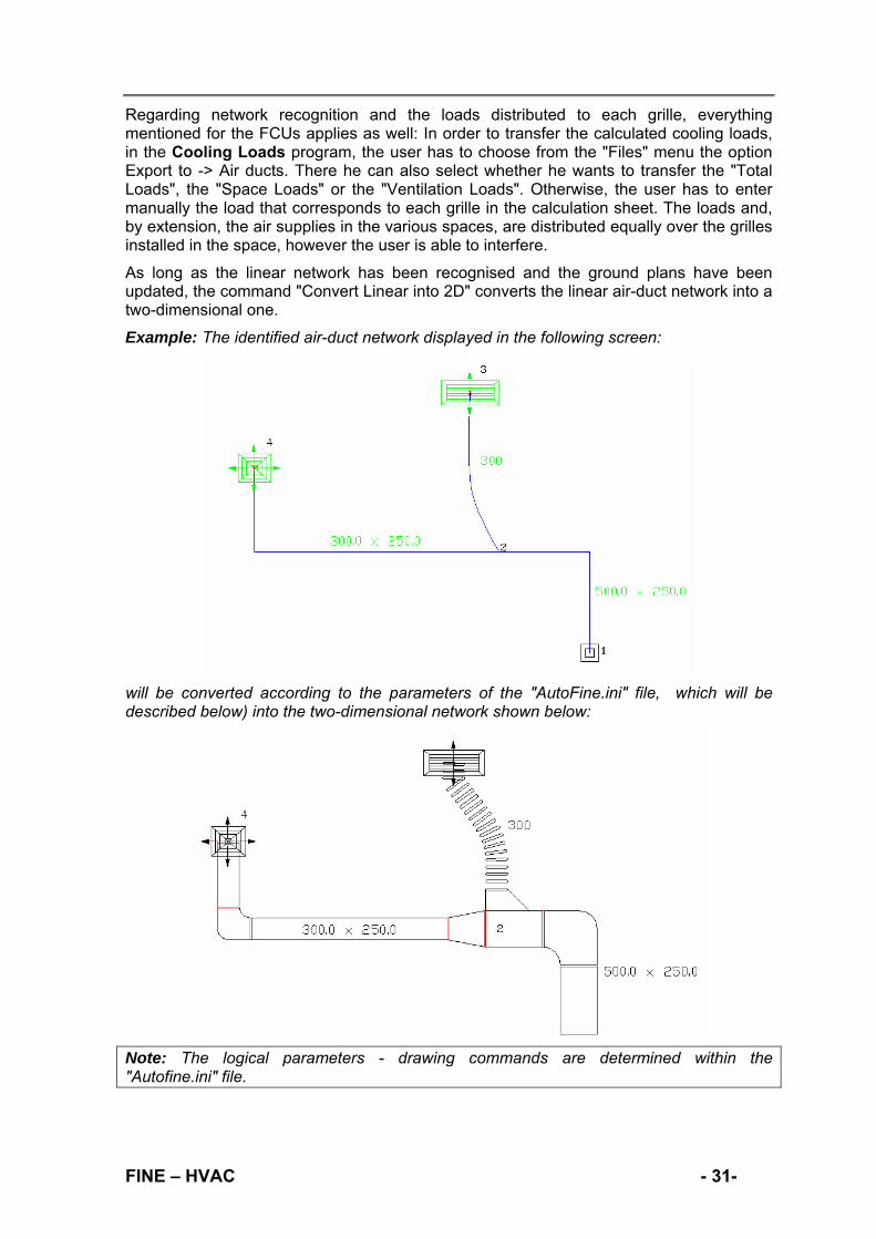
Example: The identified air-duct network displayed in the following screen:

will be converted according to the parameters of the "AutoFine.ini" file, which will be described below) into the two-dimensional network shown below:

Note: The logical parameters - drawing commands are determined within the "Autofine.ini" file.

FINE – HVAC - 31-

Apart from the automatic conversion of the linear network into two-dimensional, the program enables the independent two-dimensional air-duct drawing on the ground plans, through the "2D Design" option, activating a series of slides, each one of which is linked to an integrated drawing routine. For example, if you select an elbow, the corresponding drawing routine will ask for information about the starting point and the size of the respective angle.

Each air-duct section can be constructed either as an independent section, or consecutively to an already drawn section. In the latter case the program reads from

the previous section the direction and the initial width of the accessory. Depending on the section, the program asks for the necessary values of parameters. For example, regarding the Straight Air-duct option, which corresponds to the AERE command, the program prompts for the width, the direction and the length of the air-duct. More specifically, the options the previous command includes, are shown below:

Select air-duct endpoint Points/<Line>: Select the endpoint of an already drawn air-duct section.

Air-duct length: Insert the air-duct length, either by typing it or using the mouse.

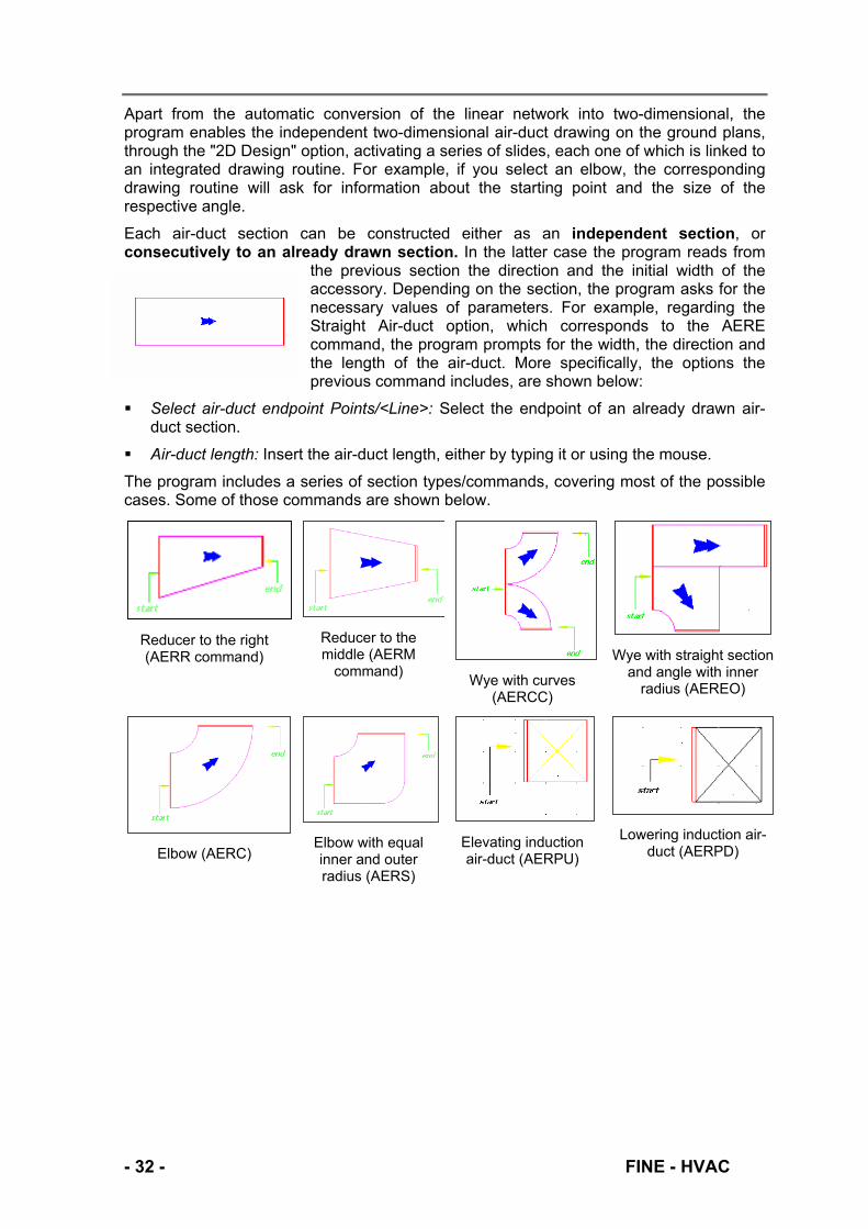
The program includes a series of section types/commands, covering most of the possible cases. Some of those commands are shown below.

Reducer to the right (AERR command)

Reducer to the middle (AERM

command) Wye with curves

(AERCC)

Wye with straight section and angle with inner

radius (AEREΟ)

Elbow (AERC) Elbow with equal inner and outer radius (AERS)

Elevating induction air-duct (AERPU)

Lowering induction air-duct (AERPD)

- 32 - FINE - HVAC

Besides the two-dimensional drawing (manually or after the automatic linear drawing conversion), Fine HVAC also enables 3D design, through rather a manual procedure, supported by the 3D drawing subsystem, which appears in the AutoNET menu. When "3D Design" is selected, a series of slides appear on the screen, each one of which is linked to a complete 3D drawing routine.

FINE – HVAC - 33-

3. Calculations

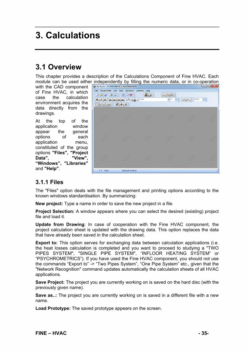
3.1 Overview This chapter provides a description of the Calculations Component of Fine HVAC. Each module can be used either independently by filling the numeric data, or in co-operation with the CAD component of Fine HVAC, in which case the calculation environment acquires the data directly from the drawings.

At the top of the application window appear the general options of each application menu, constituted of the group options "Files", "Project Data", "View", “Windows”, "Libraries" and "Help".

3.1.1 Files The "Files" option deals with the file management and printing options according to the known windows standardisation. By summarizing:

New project: Type a name in order to save the new project in a file.

Project Selection: A window appears where you can select the desired (existing) project file and load it.

Update from Drawing: In case of cooperation with the Fine HVAC component, the project calculation sheet is updated with the drawing data. This option replaces the data that have already been saved in the calculation sheet.

Export to: This option serves for exchanging data between calculation applications (i.e. the heat losses calculation is completed and you want to proceed to studying a "TWO PIPES SYSTEM", "SINGLE PIPE SYSTEM", “INFLOOR HEATING SYSTEM” or “PSYCHROMETRICS”). If you have used the Fine HVAC component, you should not use the commands “Export to” -> “Two Pipes System”, “One Pipe System” etc., given that the "Network Recognition" command updates automatically the calculation sheets of all HVAC applications.

Save Project: The project you are currently working on is saved on the hard disc (with the previously given name).

Save as..: The project you are currently working on is saved in a different file with a new name.

Load Prototype: The saved prototype appears on the screen.

FINE – HVAC - 35-

Save as Prototype: The form, which you have created and is displayed on the screen when this option is selected, can be saved as a Prototype.

Printing Prototypes: The printing prototype management window is activated.

Printing: The project issue is printed according to the selected options in "Printing Contents" and "Printing Parameters", following the print preview output.

Printing Contents: You can select the project items you want to print, as shown in the respective window.

Printing Parameters: The desired printing parameters can be selected in this window according to the procedure already mentioned in Chapter 1.

Print Preview: The complete project issue appears on the screen, exactly as it will be printed, page to page.

Export to RTF: An rtf. file containing the project items, is created.

Link to WORD: An rtf. file, containing the project items, is created (within the project directory. At the same time, the MS-Word application is activated (if it is installed in your PC).

Link to EXCEL: An excel file, containing the project items, is created. At the same time, the MS-Word application is activated (if it is installed in your PC).

Link to 4M editor: An rtf. file, containing the project items, is created. At the same time, the 4Μ text editor is activated for further editing.

Export to PDF: A PDF file containing the project items, is created (within the project directory. At the same time, the Acrobat Reader application is activated (if it is installed in your PC).

Exit: With this command, the application stops running.

3.1.2 Project Data This group of commands depends on the specific application, concerning the necessary parameters and is summarized separately for the respective application.

3.1.3 View This option follows the known windows standardization.

3.1.4 Windows Windows include a set of windows with the case study results. The main window refers to the calculation sheet which constitutes the core of each application.

3.1.4.1 Calculation Sheet

The execution of the calculations takes place in an advanced calculation environment especially designed by 4Μ for the particular needs of any specific application. It is a spreadsheet type environment with specific capabilities and facilities, tailor-made for each application. More specifically, regarding Fine HVAC applications which refer to an installation network, the calculation sheet is shown in a spreadsheet using lines corresponding to the network branches, and columns containing primary data (e.g. length) and results of calculations (e.g. water flow) for each branch. An example of such a spreadsheet for the Two Pipes Application is shown below:

- 36 - FINE - HVAC

Ι. Pipe Networks: In case the application refers to an installation network (e.g. two Pipes system, single pipe system, or even air ducts, fan coils etc.) the calculation sheet is standardised in a specific way. More specifically, the installation network is shown in a spread sheet using lines corresponding to the network branches, and columns containing primary data (e.g. length) and results of calculations (e.g. water velocity) for each branch. An example of such a sheet for the Two Pipes System is shown below:

In order to make the network understandable by the program, a specific standardization should be followed, which is more or less the same in all applications. This standardization can be easily understood with the following simple example.

Suppose we have the network which is shown in the adjacent figure. This network comprises of several branches (i.e. parts of the network), junction points and terminals (end points). Thus in this network, we have assigned arbitrary numbers to both the junction points (1,2,3) and the hydraulic terminals (4,5,6). Each junction point may be assigned to a number (from 1 to 99), a letter (lower or upper case, e.g. A, d etc) or a combination of letters and numbers (e.g. A2, AB, eZ, 2C etc.). The main restriction is that the starting point is always assigned to the number 1. Also, assigning the same number to the same network twice is not permitted for obvious reasons, with the exception of the junction point 1 for which the assignment may be repeated as desired (for networks with more than one starting points). After numbering the junction points and the terminals according to the above rule and in order to represent the network in the spreadsheet, it is enough to give a name to the various sections of the network entered in the first column of the spreadsheet. Having in mind that the order of the network sections is not important, we fill in the first column with the two junction points of each section (putting a dot in between) so that the sequence of junction points matches the direction of the water flow in the pipe. In the above example the network sections will be shown as:

Network section 1.2 2.3 2.6 3.4 3.5

FINE – HVAC - 37-

Above standardization, in spite of its several variations or extensions, is generally applied so as to contribute to an easy understanding of any application even if the user applies it initially for one particular application.

ΙΙ. Space Sheets: This standardization is encountered in applications where the related calculations refer to the spaces of the building (or, more generally, to other building entities such as the building views). Applications of such type are, for example, the calculation of Thermal losses or Cooling loads for each space separately. The spread sheet for a space is the structural element of this standardization, while all such sheets compose the complete set of spread sheets of the study.

Focusing our attention on a space spread sheet we see a series of rows corresponding to structural elements (e.g. walls W1, W3, openings O1, O2, floors F1 etc.) and columns referring to specific characteristics of these structural elements (such as Orientation, Length, Width etc.). Remaining columns are automatically updated with the results of calculations related to each row element (with deferent colour for clarity). At the lower part of the space sheet total results are also given resulting from calculations performed on all rows’ data. In the example above which is an extract of thermal losses calculation, we can see the sum of room partial losses at the bottom right in red.

Taking as a reference point the above spread sheet and ignoring initially the filled in values, we can see the columns heading zone (every column has its title and units), the zone for filling in values with a number of rows (separated with dotted lines for better supervision and clarity) and a status bar (at the bottom of the window) where helpful information appear depending on the position in the spread sheet we are in. Since the spread sheet contains usually a lot of information and is the core of the calculations in each application, it is particularly useful to have it maximized on screen by clicking on the upper arrow (located at top right of the window), so that the whole computer screen area is utilized. Next section will familiarise you with the “Calculation Sheet”, as the basic functions described therein hold good for every application.

- 38 - FINE - HVAC

Furthermore, the Calculation Sheet provides you with all the editing functions, which are described below:

First of all, as stated earlier, you can use in the frames where the Calculation Sheets appear the "Font" option for both the calculations zone (so that values appear with the desired size and style) and the headings zone (so that headings are shown to your satisfaction).

As far as the headings zone is concerned you can also increase or decrease the column width using the mouse: As long as the mouse pointer rests on the vertical line separating two adjacent columns, it takes the form of a double arrow and then by pressing (and keeping pressed) the left mouse button and dragging, the column width is increased or decreased depending on the direction of mouse movement. In the spread sheet below we can see columns having different widths:

Above, alternative supervision possibilities available to the user depend on several factors such as the resolution of the graphics card and screen size, and for this reason any possible interventions are left your discretion. For that matter, there is also the possibility of “Load Prototype” from you. Note however, that best supervision results are achieved with higher resolutions and large screens..

Access to the positions of the zone for filling in values is carried out by means of the mouse and the arrow keys of the keyboard. Moving the mouse pointer in the zone for filling in values we can see that in some columns the pointer takes the form of a vertical line (|) while in other columns it takes the form of a prohibitive traffic sign. We cannot modify the values contained in these last columns (because they result from calculations).

If we move the mouse pointer (having the form of a cross) in to a cell or small square and click the left mouse button, we’ll see that the cell contour (outline) becomes dark and we can fill in a value or modify the cell content. In the same way we can move to any other cell, or using the <Enter> key we move to the next cell below and using the <Tab> key we move to the next cell at the right and so on. Besides, in case the window width is not large enough to accommodate all columns, we can review the entire calculation sheet by manipulating it up-down or left-right using the vertically or horizontally sliding keys. In addition, when access to a column for filling values is denied the mouse pointer takes the form of a prohibitive traffic sign. This way, the user is informed that the quantity under examination is a derivative one i.e. resulted automatically from calculations.

FINE – HVAC - 39-

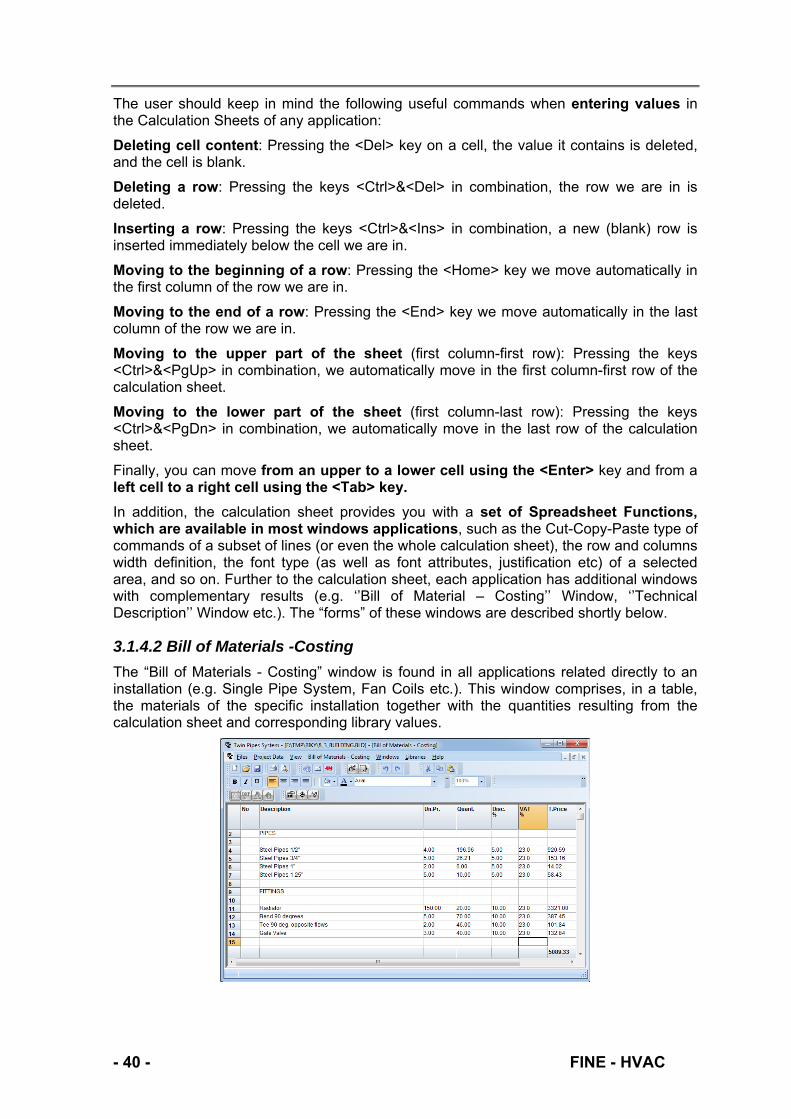
The user should keep in mind the following useful commands when entering values in the Calculation Sheets of any application:

Deleting cell content: Pressing the <Del> key on a cell, the value it contains is deleted, and the cell is blank.

Deleting a row: Pressing the keys <Ctrl>&<Del> in combination, the row we are in is deleted.

Inserting a row: Pressing the keys <Ctrl>&<Ins> in combination, a new (blank) row is inserted immediately below the cell we are in.

Moving to the beginning of a row: Pressing the <Ηοme> key we move automatically in the first column of the row we are in.

Moving to the end of a row: Pressing the <End> key we move automatically in the last column of the row we are in.

Moving to the upper part of the sheet (first column-first row): Pressing the keys <Ctrl>&<PgUp> in combination, we automatically move in the first column-first row of the calculation sheet.

Moving to the lower part of the sheet (first column-last row): Pressing the keys <Ctrl>&<PgDn> in combination, we automatically move in the last row of the calculation sheet.

Finally, you can move from an upper to a lower cell using the <Εnter> key and from a left cell to a right cell using the <Tab> key.

In addition, the calculation sheet provides you with a set of Spreadsheet Functions, which are available in most windows applications, such as the Cut-Copy-Paste type of commands of a subset of lines (or even the whole calculation sheet), the row and columns width definition, the font type (as well as font attributes, justification etc) of a selected area, and so on. Further to the calculation sheet, each application has additional windows with complementary results (e.g. ‘’Bill of Material – Costing’’ Window, ‘’Technical Description’’ Window etc.). The “forms” of these windows are described shortly below.

3.1.4.2 Bill of Materials -Costing

The “Bill of Materials - Costing” window is found in all applications related directly to an installation (e.g. Single Pipe System, Fan Coils etc.). This window comprises, in a table, the materials of the specific installation together with the quantities resulting from the calculation sheet and corresponding library values.

- 40 - FINE - HVAC

Materials are listed as items (e.g. pipes, fittings etc.) in the rows of the table, while the table columns contain information such as "unit price", "quantity", "discount %", "VAT" and "Total Price". Calculations are performed automatically and the results appear in the last column. You can edit the bill of materials-costing table in a similar way as for the calculations sheet. When the "Bill of Materials" window is active, then the option with the title name appears in the main menu together with the two secondary options "Offer Parameters" and "Printing Parameters" providing more options to the user.

3.1.4.3 Technical Description

The “Technical Description” window supports composition of the project’s technical description and it is automatically updated when a change in the “Calculation method” is made.

Making the selection “Technical Description” the corresponding title window in yellow background appears updated with the project’s results (where word-parameters exist). When the Technical Description window is activated, an additional option in the main menu (just above the “Windows” option) is appeared with the name “Technical Description”. Choosing “Prototype Selection” from this menu the prototype management window will appear on our screen.

Selecting the corresponding prototype (with the help of the mouse and using the “Load” key), the corresponding text appears in the Technical description window (also in yellow background and with updated results of the project).

FINE – HVAC - 41-

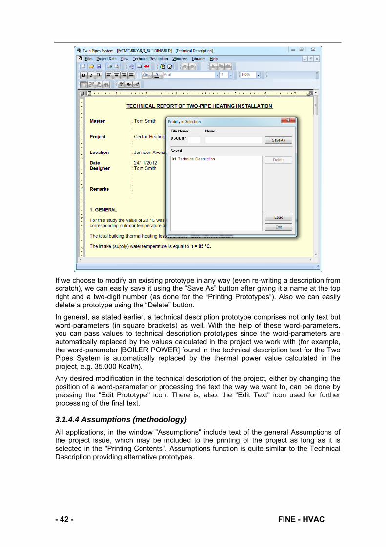
If we choose to modify an existing prototype in any way (even re-writing a description from scratch), we can easily save it using the “Save As” button after giving it a name at the top right and a two-digit number (as done for the “Printing Prototypes”). Also we can easily delete a prototype using the “Delete” button.

In general, as stated earlier, a technical description prototype comprises not only text but word-parameters (in square brackets) as well. With the help of these word-parameters, you can pass values to technical description prototypes since the word-parameters are automatically replaced by the values calculated in the project we work with (for example, the word-parameter [BOILER POWER] found in the technical description text for the Two Pipes System is automatically replaced by the thermal power value calculated in the project, e.g. 35.000 Kcal/h).

Any desired modification in the technical description of the project, either by changing the position of a word-parameter or processing the text the way we want to, can be done by pressing the "Edit Prototype" icon. There is, also, the "Edit Text" icon used for further processing of the final text.

3.1.4.4 Assumptions (methodology)

All applications, in the window "Assumptions" include text of the general Assumptions of the project issue, which may be included to the printing of the project as long as it is selected in the "Printing Contents". Assumptions function is quite similar to the Technical Description providing alternative prototypes.

- 42 - FINE - HVAC

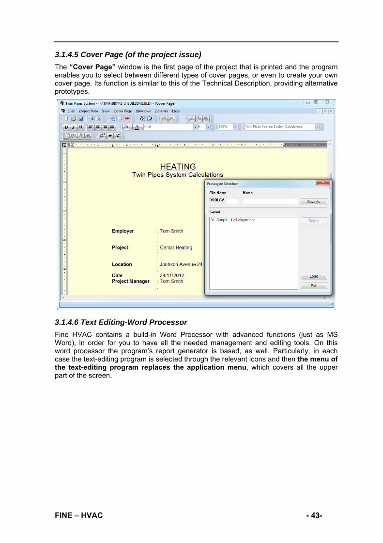
3.1.4.5 Cover Page (of the project issue)

The “Cover Page” window is the first page of the project that is printed and the program enables you to select between different types of cover pages, or even to create your own cover page. Its function is similar to this of the Technical Description, providing alternative prototypes.

3.1.4.6 Text Editing-Word Processor

Fine HVAC contains a build-in Word Processor with advanced functions (just as MS Word), in order for you to have all the needed management and editing tools. On this word processor the program’s report generator is based, as well. Particularly, in each case the text-editing program is selected through the relevant icons and then the menu of the text-editing program replaces the application menu, which covers all the upper part of the screen.

FINE – HVAC - 43-

The option groups of the text editing program consist of the following: "Files", "Edit", "View", "Insert", "Font’’, "Paragraph’’, "Table" and "Other options". In detail, the commands of the text-editing program are divided in the groups Editing Commands (Cut, Copy, Paste, Delete, Paste Special, Edit Picture, Undo, Redo, Select All, Repaginate etc.), View Commands (Page Mode, Fitted View, Ruler, Tool Bar, Zoom etc.), Insert (Add) Commands (Insert Break, Page Break, Section Break, Column Break, Embed Picture, Link Picture, Ole Object etc.), Font Commands (Normal, Bold, Underline, Italic, Superscript, Text Colour etc), Paragraph Commands (Normal, Centre, Justify, Indent Left, Border and Shading, Bullet, Numbering, Set Tab etc.), Table Commands (Insert Table, Insert Row, Merge Cells, Header Row, Cell Vertical Align etc) and More Options (Search, Replace, Snap to Grid, Background Picture etc.).

Besides, when the text-editing program is "active", there is a "ruler" in the upper part of the text window, which shows the distances with the "guides" and the tab symbols.

In general whatever applies to Word applies here too. In order to exit the Word Processor and return to the previous desktop, you select "Exit" in the first menu under "File".

As mentioned before, the Report Generator of the program is based on the above described word processor. In order to define a report, you have to insert the variables (parameters) of any application in the right position into the text (i.e. under the titles). For example the parameter ''net_sec'' should be placed under the title “Branch of Network”. All these parameters take automatically the exact values that have been calculated by the program.

- 44 - FINE - HVAC

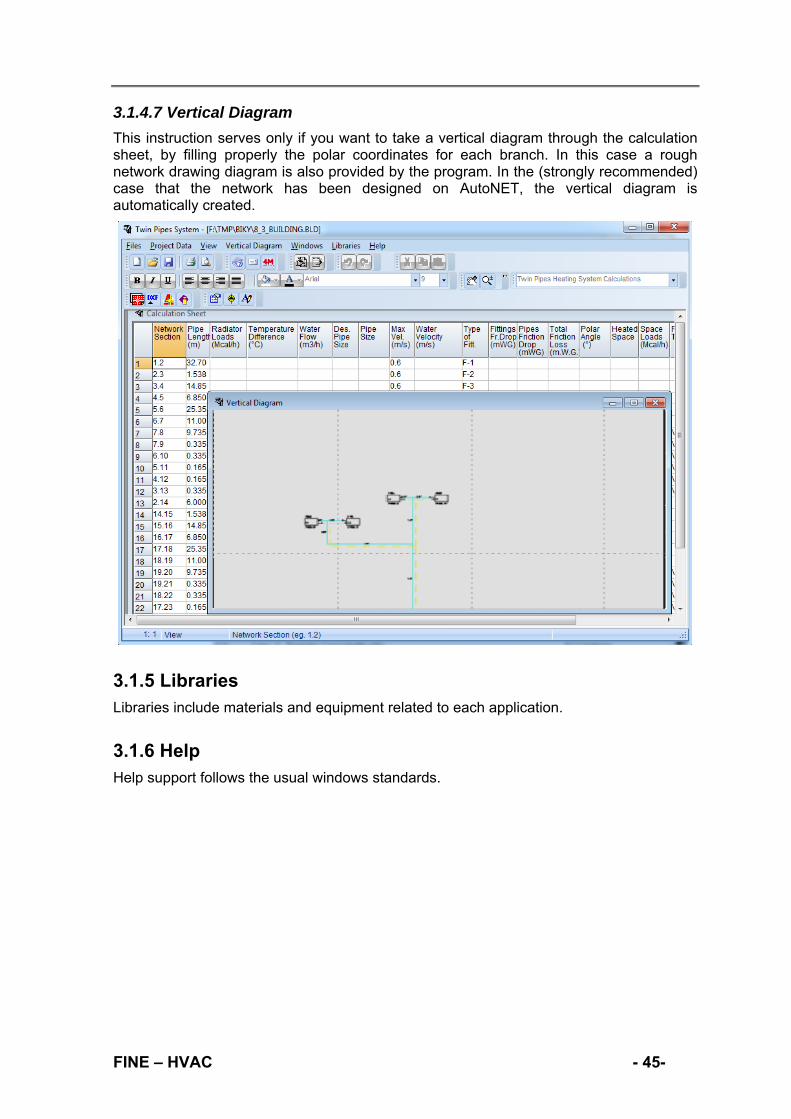
3.1.4.7 Vertical Diagram

This instruction serves only if you want to take a vertical diagram through the calculation sheet, by filling properly the polar coordinates for each branch. In this case a rough network drawing diagram is also provided by the program. In the (strongly recommended) case that the network has been designed on AutoNET, the vertical diagram is automatically created.

3.1.5 Libraries Libraries include materials and equipment related to each application.

3.1.6 Help Help support follows the usual windows standards.

FINE – HVAC - 45-

3.2 Heating The Heating part consists of four applications which function either independently or in conjunction with each other and/or the Fine HVAC Component. These applications are listed below:

Thermal Losses: Heat losses are calculated in each building floor and room. This procedure usually comprises the first step of a heating project.

Two Pipes System: All the necessary calculations for the installation of a Two Pipe Heating System are made and the required equipment is selected (radiators, pipes, boiler, burner, circulator, safety device, tank, chimney etc.).

Single Pipe System: All the necessary calculations for the installation of a Single Pipe Heating System are made and the required equipment is selected (radiators, pipes, boiler, burner, circulator, safety device, tank, chimney etc.).

Infloor Heating System: All the necessary calculations for the installation of an Infloor System are made and the required equipment is selected (radiators, pipes, boiler, burner, circulator, safety device, tank, chimney etc.).

3.2.1 Thermal Losses By executing the Thermal Losses application, the main menu screen appears, including the main menu options “Files", "Project Data", "View", “Windows”, "Libraries" and "Help". “Files”, “View” and “Help” and most of the other options are following the rules described in the previous section. The rest is described in short in the following paragraphs.

3.2.1.1 Project Data

There are three basic data categories of the project: Project info, Building parameters and Structural elements. When “Building parameters” is selected, a window appears presenting a list of items concerning mainly the building and some additional data. These items and the values which should be given to them are explained right below, exactly in the same order in which they appear in the window:

1) Building parameters tab

City: Select from the list that opens (by pressing F11 or the appropriate button into the field) the city you want (you can add and use your own cities in Libraries -> Outer Winter Temperatures).

Design external temperature (ºC): You can see (by pressing F11 or the appropriate button into the field) the library list containing climatologic data for the cities, and either select a value from it or type directly the desired temperature value.

Desired Indoor temperature (ºC): You select from the list or type the more typical indoor temperature, in case there are more than one value. This value can be selectively edited in the fields of the spaces where a different temperature is required.

FINE – HVAC - 47-

Not-heated spaces temperature (ºC): The temperature of the building spaces which are not heated (e.g. staircase) should be typed in this field.

Soil temperature (ºC): The soil temperature should be typed in this field.

Annual mean external temperature (ºC): You can see (by pressing F11 or the appropriate button into the field) the library list containing climatologic data for the cities, and either select a value from it or type directly the desired temperature value.

Calculation Method: You have the option to choose between the older (1977) or the newer (1983) DIN standard, the European norm EN12831, the American ASHRAE HB 2001 or HB 2013 method and the ASHRAE Ships (Merchant or Naval) method.

Vessel type: If the ASHRAE Ships method has been chosen, select the type of the vessel.

Default space increment (%): This value is used only in the case of non-automatic increase calculations (see last option), as it is simply stated for every room, can be selectively modified by the user.

Number of levels (floors): You define the number of the levels of the building.

Default height (m): You type a default height for each level. This value can be selectively edited in the fields of the spaces where is required.

Energy units: You have the option to choose between Kcal/h or Watts for the results.

Floor slab depth (m): If the floor slab is beneath ground level, you type its depth (used only in ASHRAE HB 2013).

Floor on the ground level: The number of the floor which is on the ground level (e.g. 2nd floor) must be filled, so that the floor distances and, therefore, the rift increase due to height (DIN 1983) can be automatically calculated.

Heating system efficiency factor: You type the efficiency factor of the heating system.

Air exchange rate/hour: You select (by pressing F11 or the appropriate button into the field) the number of air exchanges per hour depending on the type of the room or type it directly. This value can be selectively edited in the fields of the spaces where is required.

Rotation angle: If you want to change the orientation of the building, you can rotate it to a specific angle through selecting it from the list that opens.

2) DIN 77-83 tab

This tab is completed if you want to use the DIN77 or DIN83 methodology.

Building characteristic number Hk: It depends on how much the building is exposed to winds (see auxiliary table).

Shut-Down period: One of the 3 options should be selected: "0 break hours", "8-12 break hours" or "12-16 break hours".

Space characteristic number R: Depending on the ratio of the internal to external openings, an auxiliary table, based on the selected DIN, appears.

Automatic Increment Calculations: By checking the box, the increase percentage is automatically modified in every room in combination with the above selected DIN. Therefore, the increase percentage due to exposure, breaks and walls will be displayed analytically for each space.

3) EN 12831 tab

- 48 - FINE - HVAC

This tab is completed if you want to use the EN12831 methodology.

Area of floor slab (m²): You type the area of the considered floor slab. For a whole building, it is the total ground floor area. For part of a building, it is the ground floor area under consideration.

Perimeter of floor slab (m): You type the perimeter of the considered floor slab. For a whole building, it is the total perimeter. For part of a building, it includes only the length of external walls separating the heated spaces under consideration from external environment.

Building volume (m³): You fill in the volume of the building.

Building exhaust air flow rate Vex (m³/h): If there is ventilation system in the building, in this cell you fill in the exhaust air flow rate.

Building supply air flow rate Vsu (m³/h): If there is ventilation system in the building, in this cell you fill in the supply air flow rate.

Correction factor for influence from annual variation of external temperature fg1: You type a value for the correction factor taking into account the influence from annual variation of external temperature. Default value is 1.45.

Correction factor for influence from ground water Gw: You select a value for the correction factor, taking into account the influence from ground water. Default values are either “1” if the distance between the assumed water table and the floor slab is more than 1 m, or “1.15” if the distance is less than 1 m.

Air exchange rate/hour at 50 Pa: You select (by pressing F11 or the appropriate button into the field) or type directly the air exchange rate at 50 Pa pressure difference between inside and outside per hour.

Shielding coefficient ei: You select (by pressing F11 or the appropriate button into the field) or type directly the shielding coefficient depending on the exposure of the building.

Supply air temperature tsu: You type the supply air temperature into the heated space (either from the central air heating system, from a neighbouring heated or unheated space or from the external environment). This value can be selectively edited in the fields of the spaces where is required.

Calculation of reheating: In case there is a reheating system in the building, you check this box.

Correction factor for reheating: You select (by pressing F11 or the appropriate button into the field) or type directly the correction factor for reheating which depends on the reheat time and the assumed drop of the internal temperature during setback.

Ceiling height correction >5m: For buildings with ceilings which have a height greater that 5 m, you check this box.

Ceiling height correction factor fh,i: For buildings with design heat losses ≤60 W/m² of floor area, for spaces with high ceilings a correction factor is used. You select (by pressing F11 or the appropriate button into the field) the correction factor depending on the height of the heated space.

Efficiency of heat recovery system nv: In case there is a heat recovery system, you type its efficiency on exhaust air.

FINE – HVAC - 49-

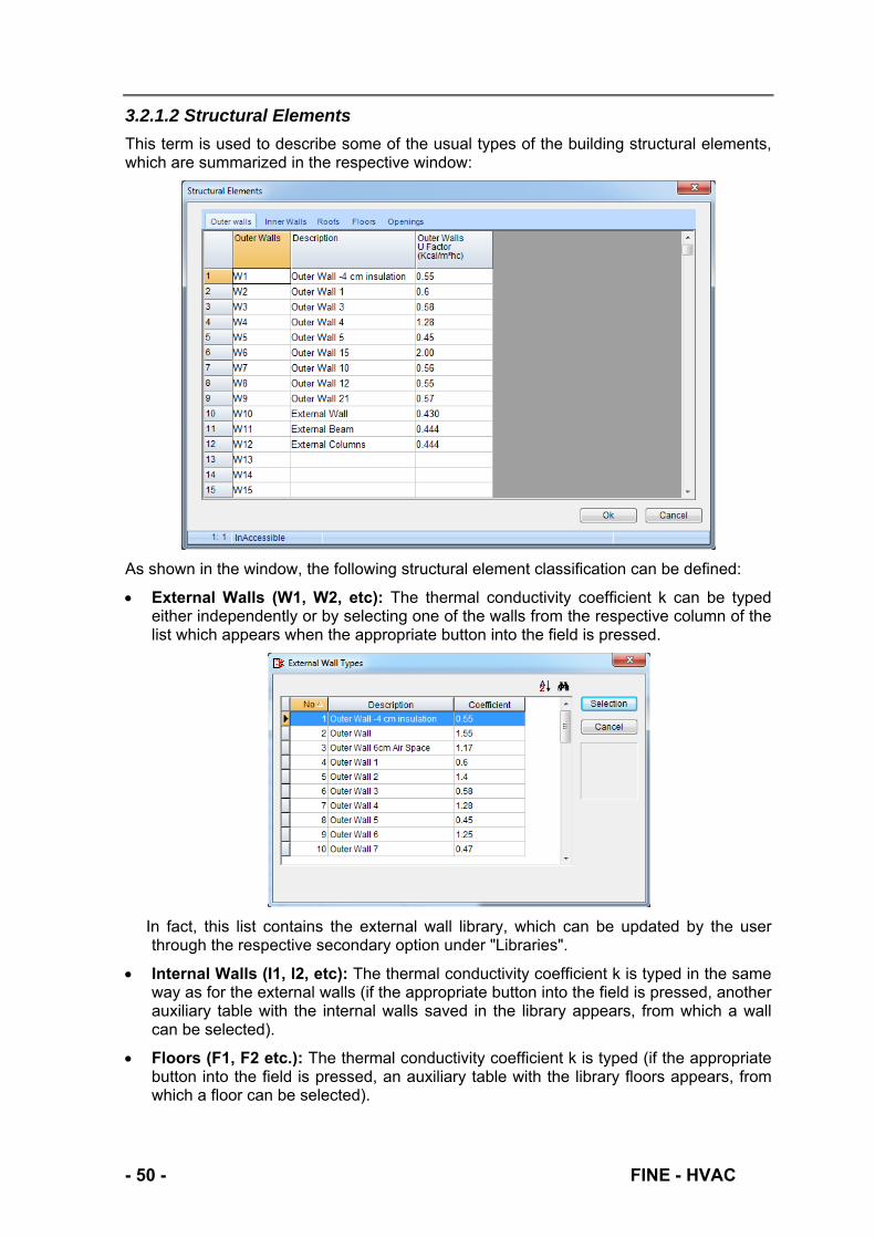
3.2.1.2 Structural Elements

This term is used to describe some of the usual types of the building structural elements, which are summarized in the respective window:

As shown in the window, the following structural element classification can be defined:

External Walls (W1, W2, etc): The thermal conductivity coefficient k can be typed either independently or by selecting one of the walls from the respective column of the list which appears when the appropriate button into the field is pressed.

In fact, this list contains the external wall library, which can be updated by the user through the respective secondary option under "Libraries".

Internal Walls (I1, I2, etc): The thermal conductivity coefficient k is typed in the same way as for the external walls (if the appropriate button into the field is pressed, another auxiliary table with the internal walls saved in the library appears, from which a wall can be selected).

Floors (F1, F2 etc.): The thermal conductivity coefficient k is typed (if the appropriate button into the field is pressed, an auxiliary table with the library floors appears, from which a floor can be selected).

- 50 - FINE - HVAC

Ceilings (or Roofs) (C1, C2 etc.): The thermal conductivity coefficient k is typed (if the appropriate button into the field is pressed, an auxiliary table with the library ceilings appears, from which a ceiling can be selected).

Openings (O1, O2 etc.): You can type the opening dimensions (width, height), the thermal conductivity coefficient k (if or the appropriate button into the field is pressed, the auxiliary library table appears, from which a window can be directly selected), the air penetration coefficient a (infiltration) and the sheets number (one, two etc.). The data which will remain blank can be filled in later within the losses calculation sheet.

3.2.1.3 Thermal Losses Calculation Sheet

The calculation sheets for space losses are included in the respective building floor sheets. If you select one of the floors, a list will appear containing the respective losses sheets for the floor spaces along with their management toolbar:

When a new project is created this list is blank. When you enter this list (with the mouse) and click the icon (with the “+” sign on the lower side) in the menu or press the key <Ins>, a small window appears, where the name of the desired space should be typed (e.g. Kitchen, Bathroom etc.). If you press “OK” this space Enters the list and all you have to do is type the space dimensions in the thermal losses sheet. In the same way, if you click the icon Delete Space (with the “x“ sign) or even press <Del> on the keyboard, after

FINE – HVAC - 51-

selecting the name of the space, the specific space is deleted. By pressing <Ctrl>&<I> or clicking the icon of insertion (with the “+” sign in the middle) a new space is inserted.

To every space (left) corresponds a Losses Sheet (right), where up to 60 different structural elements can be inserted and which can be separated in two parts:

On the upper part, each row of the losses sheet corresponds to a structural element while each column refers to the data which are going to be inserted or are going to result automatically during the process of the sheet completion. Instructions about entering these data are displayed in the status bar. For each row, the first column which refers to some type of structural element should be filled first. If a typical element is concerned, the corresponding data of the building typical data sheet are automatically filled.

For each row-structural element the following must be defined: The orientation, the indication "Subtracted" (by S) since it considers an element that can be removed from the element just above this one (such as windows, columns and beams), the thickness (optional), the length and the height of the structural element, the number of similar surfaces, the thermal conductivity coefficient and the temperature difference. The openings are removed automatically under the following conditions:

The openings must be entered under the walls to which they belong.

A common orientation should be entered for the openings and the respective walls (or "I" if it is about internal openings on internal walls (non heated), "C" for horizontal openings/skylights, "P" for Pilotis Roof - attention for Pilotis you enter Ceiling, e.g. C1 and not Floor).

The indication "S" (Subtracted) should exist in the correspondent column (for the openings it is inserted automatically at the beginning).

Note: For Floors that are adjacent to the ground you do not fill in the second column, while when the Floor is above a non heated space you fill "I". For Roof to external space (or openings on the roof) you enter "C", to internal "I" and to pilotis "P".

When the “ASHRAE Ships” method is selected, the extra column “Adjoining space” has to be filled in.

- 52 - FINE - HVAC

On the bottom side of the screen appear data which refer to the overall sheet: These are the total increase, the losses due to slots or air changes, the total losses due to thermal conductivity and the total space losses, as well as some additional data that are used as a link to the applications of Cost Distribution and Single Pipe System. All these data are organized in 3 columns, the first two of which refer to parameters and the third to total results about the space. Keep in mind that depending on the methodology selection you make in the “Building Parameters”, different data are shown. More specifically, if you select, for example, the DIN methodology:

In the first column appear the increase percentages due to exposure and breaks, as well as the desired increase percentage which can be modified. The total increase percentage automatically becomes equal to the value that exists on the general data sheet, which can be modified by the user. You can be based either on your judgement, or on the method (DIN) increase value. The last one is displayed on the right side in brackets depending on the selected methodology and consists of two components: The increase due to exposure ZH and the general increase ZD due to breaks (ZU) and Cold Walls (ZA) (ZD=ZU+ZA).

Lower on the first column, the values R, H and ZΓ are shown that are typed under the “Building Parameters”. These values are taken into consideration automatically for the calculation of the losses due to slots, losses that are displayed in the middle of the 3rd column.

You can interfere to the calculation as you can change the values R (or r), H and ZΓ. In the case of the DIN83 the coefficient Η is increased automatically when the height is over 10 meters using the factor eGA. If any of these values are zero, the losses due to slots are also zero, which must be performed when there is forced ventilation (therefore the space is over pressurised).

In the second column, the space dimensions which are on the upper part (Length, Width, Height) are used for the calculation of the adjacent surface (for the calculation of the increase due to breaks) and the losses due to air changes. The calculation of the latter is performed as long as the number of changes per hour is entered in the row right below.

Below you can fill the symbolic name of the Property (e.g. 1A, 1B, A1, 1IS or any other name you wish).

The circuit topology (to enable linking to the Single Pipe System program) can be defined in the last two rows. Specifically, it is necessary to insert two numbers:

The number of the vertical pipe and the circuit which passes through the specific space (number the circuits by level and vertical pipes starting from 1). For example, if the first vertical pipe of the building and the second circuit of the vertical pipe pass through the specific space, you should type 1.2 in the specific level.

The radiator serial number in the circuit (number the radiators in each circuit starting from 1). If there is more than one radiator in the same space, their serial number is inserted with a full stop (e.g. 1.2 or 2.4 etc). Note that in case of a twin pipes system no entering is required, because you can call the load of any space directly from there.

FINE – HVAC - 53-

Notes:

In case two different circuits pass through one space, it is recommended to divide the space in two parts (e.g. Living-room part Α, Living-room part Β) in order to define the corresponding circuit in each part. If this is not possible, the user can interfere afterwards to the Single Pipe System and make the required changes.

In case you use the Fine HVAC and you have designed the circuits in the ground plan, it is obvious that you do not need to fill the two previous fields since the topology is given and the program takes it automatically into consideration.

Finally, in the third column, the total results of the space thermal losses are presented. First of all, the Total Losses due to Thermal Conductivity are presented, that are the sum of the losses in the last column of the losses sheet (space losses). The absolute value of the increase, which corresponds to the percentage of the increase of the first column, is presented below. The sum of the two previous values provides the Final Losses due to Thermal Conductivity (Final Thermal Losses) which are displayed right below. After that, the space losses due to Openings Slots and Ventilation are presented (only one of them is provided with a value). Finally, the sum of all previous values of column 3, which provides the Total Space Losses, is presented in the lower part.

Also, the program enables the copying of each floor or space to any other, through the usual copy-paste window functionality.

3.2.1.4 Circuits-Radiators-Properties

The window “Circuits-Radiators-Properties” presents a list of the building spaces with the circuits-radiators which correspond to each space, as well as the properties to which they belong. With the help of this window, you can control the above data and detect any omissions. This window is extremely useful in case the program displays a message about an “Unspecified Property” or “Incomplete Circuits” during the creation of the link files Single Pipe System (or Infloor Heating System).

3.2.1.5 Overall Data of Losses

A list appears with the spaces per level and a number with their names and their losses, as well as the side and total losses sums.

3.2.1.6 Properties Thermal Losses

A list appears with the Properties and losses Qol, (Total, due to Openings and Slots respectively).

- 54 - FINE - HVAC

3.2.1.7 Energy Analysis

The program has the ability of Energy Analysis by the Degree Day Method. Based on the results of the thermal losses, the program calculates the annual energy consumption required for the main cities based on the Degree Days (from weather data) which have been measured for each city on annual basis and for defined temperature limits. These data are in the "Libraries" and can be updated by the user.

3.2.1.8 Libraries

The libraries refer to structural element types, as well as to temperature data. They can be easily updated by you and therefore you can enter your own data exactly as you desire.

FINE – HVAC - 55-

3.2.2 Two Pipes System By executing the Two Pipes Heating System application, the main menu screen appears, including the options "Files", "Project Data", "View", “Windows”, "Libraries" and "Help". “Files”, “View” and “Help”, as well as a part of the window sub-options (cover page, assumptions, technical descriptions, bill of materials etc.) follow the usual windows standards and the description provided in section 3.1. The rest are described in short in the following paragraphs.

3.2.2.1 Project Data

This pertains to the project basic data, which are divided into Project info (project headings) and Network data. Network data concern:

Inlet Water temperature: Enter the inlet water temperature in C (the return temperature is calculated automatically)

Radiators Temperature Drop: Enter the radiators temperature drop (usual value Dt=15 C).

Room temperature: Enter the room temperature (usually 20 degrees Celsius).

Main pipe type: Select the pipe type of the main pipes (e.g. copper pipe).

Main pipes roughness factor: Roughness factor is entered automatically, depending on the pipe type selected, but you can easily modify it. The measurement unit used by the program is μm.

Secondary pipes type: Select the pipe type of the secondary pipes (in case two types are used, e.g. copper pipe for the vertical pipes and plastic pipes for the horizontal piping).

Secondary pipes roughness factor: The roughness factor is entered automatically, depending on the pipe type you have selected, but you can easily modify it. The measurement unit used by the program is μm.

Maximum water velocity: Enter the maximum desired water velocity limit (based on which the cross-sections are calculated).

Friction limit (mwg/m): Enter the friction limit per length of the piping in mwg/m.

Number of circulators: In case you have more than one circulator, enter their number here so as to be able to use them in the Calculation sheet and the Circulator calculation.

Energy units: Select the unit system (Kcal/h or watt).

Expansion tank type: Select between open and – more often used – closed expansion tank.

Temperature drop per meter: If you do not have ideally insulated pipes, enter in this field the temperature drop per meter of the length of piping (in °C/m).

Chimney calculations according to EN 13384.01: If you check this box, you can calculate the chimney according to the European norm EN 13384.01.

Building geodetic height in relation to sea level: Enter the geodetic height of the building.

Analytical calculation of contained water in the system: If you check this box, you can calculate in detail the contained water in the system.

- 56 - FINE - HVAC

Combi system: This box is checked when you have several boilers and circulators in the network. In this case, you check this box and type the “Number of circulators” in the same window so as to calculate them.

Fuel Type: Select the fuel that is used (oil, natural gas, LPG etc.).

3.2.2.2 Calculation Sheet

Following the standardization described earlier, each row of this sheet corresponds to a different network section while each column refers to data that will be filled out or will ensue automatically during the procedure of completing data.

The space load is taken immediately (by inserting the level and space number (e.g. 1.2) provided that a link to losses has been established and the respective supply corresponds to the total required supply for the space. If there is more than one radiator in the same space, the designer should intervene by distributing the load accordingly. The respective radiator is calculated for the radiator type selected through the library.

Based on the supply in each network section and given the maximum velocity that corresponds to this section, the cross-section of the section pipe is established. Despite all this, the designer may give another standardized diameter, by selecting (through the 6th column) the list of standardized diameters from the library that appears on the screen. In whatever way the section has been defined, the effective water velocity and the pressure drops (see respective columns) of the piping and fittings in the respective section of the network will be exactly calculated. The fittings are completed in each section separately, opening the respective fittings window.

At this point, the fitting numbers for each type of accessory must be given or their combination. There is also the option to assign an increasing number system for the fittings (in the upper row) for avoiding the repeated filling out of the same.

In the case of typical (similar) sections it is possible to recall them (with their name from the first column) in order to automatically transfer them.

FINE – HVAC - 57-

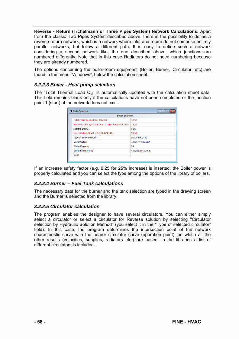
Reverse - Return (Tichelmann or Three Pipes System) Network Calculations: Apart from the classic Two Pipes System described above, there is the possibility to define a reverse-return network, which is a network where inlet and return do not comprise entirely parallel networks, but follow a different path. It is easy to define such a network considering a second network like, the one described above, which junctions are numbered differently. Note that in this case Radiators do not need numbering because they are already numbered.

The options concerning the boiler-room equipment (Boiler, Burner, Circulator, etc) are found in the menu “Windows”, below the calculation sheet.

3.2.2.3 Boiler - Heat pump selection

The "Total Thermal Load Qol" is automatically updated with the calculation sheet data. This field remains blank only if the calculations have not been completed or the junction point 1 (start) of the network does not exist.

If an increase safety factor (e.g. 0.25 for 25% increase) is inserted, the Boiler power is properly calculated and you can select the type among the options of the library of boilers.

3.2.2.4 Burner – Fuel Tank calculations

The necessary data for the burner and the tank selection are typed in the drawing screen and the Burner is selected from the library.

3.2.2.5 Circulator calculation

The program enables the designer to have several circulators. You can either simply select a circulator or select a circulator for Reverse solution by selecting ''Circulator selection by Hydraulic Solution Method'' (you select it in the “Type of selected circulator” field). In this case, the program determines the intersection point of the network characteristic curve with the nearer circulator curve (operation point), on which all the other results (velocities, supplies, radiators etc.) are based. In the libraries a list of different circulators is included.

- 58 - FINE - HVAC

3.2.2.6 Expansion Tank and Chimney calculations

In order to select an Expansion Tank you should fill properly the parameters shown in the dialog. The required volume comes up automatically and the effective volume finally appears, if the dimensions (length, width, height) are typed in the following fields.

Regarding the Chimney, the program provides the option for very detailed calculations through mathematical curves.

3.2.2.7 Network Drawing

The (numbered) network drawing is shown on the screen, provided that polar coordinates have been inserted in every network branch (see calculation sheet).

FINE – HVAC - 59-

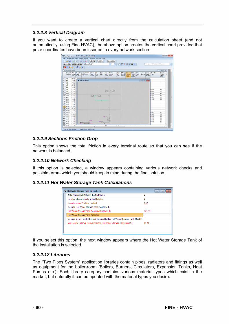
3.2.2.8 Vertical Diagram

If you want to create a vertical chart directly from the calculation sheet (and not automatically, using Fine HVAC), the above option creates the vertical chart provided that polar coordinates have been inserted in every network section.

3.2.2.9 Sections Friction Drop

This option shows the total friction in every terminal route so that you can see if the network is balanced.

3.2.2.10 Network Checking

If this option is selected, a window appears containing various network checks and possible errors which you should keep in mind during the final solution.

3.2.2.11 Hot Water Storage Tank Calculations

If you select this option, the next window appears where the Hot Water Storage Tank of the installation is selected.

3.2.2.12 Libraries

The "Two Pipes System" application libraries contain pipes, radiators and fittings as well as equipment for the boiler-room (Boilers, Burners, Circulators, Expansion Tanks, Heat Pumps etc.). Each library category contains various material types which exist in the market, but naturally it can be updated with the material types you desire.

- 60 - FINE - HVAC

3.2.3 Single Pipe System The main menu options are divided into the groups "Files", "Project Data", "View", “Windows”, "Libraries" and "Help". “Files”, “View” and “Help” and most of the other options are quite similar to the “twin pipe heating” application (they are discussed in detail in paragraphs 3.1.1, 3.1.3 and 3.1.6 respectively). The rest are described in short in the following paragraphs.

3.2.3.1 Project Data

This pertains to the project basic data, which are divided into Project info (project headings) and Network data. Network data concern:

Space Temperature (C): Enter the desired space temperature in C (usually 20 C).

Inlet water temperature (C): Enter the inlet water temperature in C (the return temperature is calculated automatically)

Water Temperature drop per level (%): Enter (if desired) a percentage of temperature drop per level, due to minor losses in the vertical pipe of the installation.

Water Temperature drop at the circuits (C): Enter the temperature drop at the circuits (usually 15 C). This need to be entered only if the equal temperature drops method is used.

Maximum velocity limit for the central pipes (m/s): Enter the maximum water velocity limit in the main pipes.

Maximum water velocity limit for the circuits (m/s): Enter the maximum desired water velocity limit at the circuits. In general, for Single Pipe System circuits with copper or plastic pipes on the floor, water velocity should be between w=1.0-1.2 m/s.

Main pipe types: Select the pipe type of the main pipes (e.g. copper pipe)

Main pipes roughness factor: The roughness factor is entered automatically, depending on the pipe type you have selected, but you can easily modify it. The measurement unit used by the program is μm.

Circuits pipes type: Select, to enter the pipes type for the circuit pipes (e.g. copper pipe).

Circuit pipes roughness factor: The roughness factor is entered automatically, depending on the pipe type you have selected, but you can easily modify it. The measurement unit used by the program is μm.

Circuits desired pipe size: Enter the desired circuit pipes size (diameter). Initially, this will be the same for all circuits. Diameter may be selectively modified for specific circuits in the calculation sheets (although in practice, most of the times loops with the same diameter are used).

Desired switch Regulating (%): Enter the initial setting of the radiators switches (usually 50%). For the last radiator of a circuit, most engineers set the switch to 100%. If the program works with Fine HVAC, this setting is entered automatically.

Switch Equivalent Length: Enter the equivalent length of the switch (in m). By default, the program considers that there is one switch for every radiator.

Branch Equivalent Length: Enter the equivalent length of the branch (in m). By default, the program considers that there are two branches for every circuit (inlet & return).

FINE – HVAC - 61-

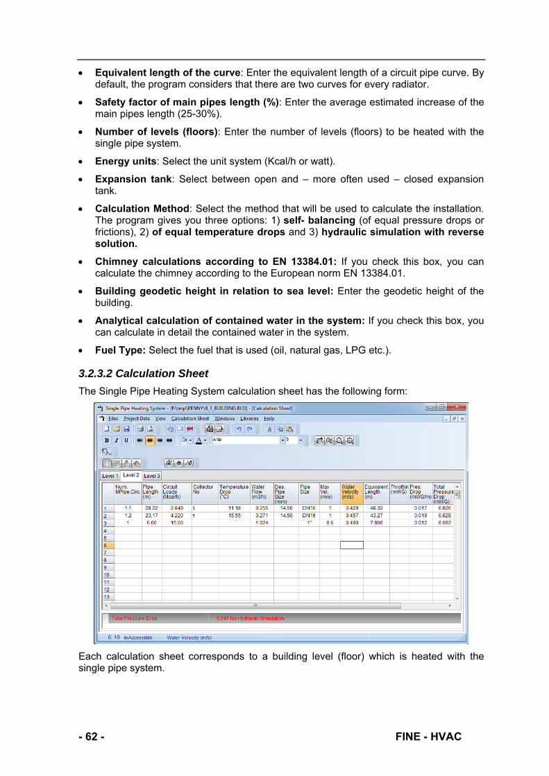
Equivalent length of the curve: Enter the equivalent length of a circuit pipe curve. By default, the program considers that there are two curves for every radiator.

Safety factor of main pipes length (%): Enter the average estimated increase of the main pipes length (25-30%).

Number of levels (floors): Enter the number of levels (floors) to be heated with the single pipe system.

Energy units: Select the unit system (Kcal/h or watt).

Expansion tank: Select between open and – more often used – closed expansion tank.

Calculation Method: Select the method that will be used to calculate the installation. The program gives you three options: 1) self- balancing (of equal pressure drops or frictions), 2) of equal temperature drops and 3) hydraulic simulation with reverse solution.

Chimney calculations according to EN 13384.01: If you check this box, you can calculate the chimney according to the European norm EN 13384.01.

Building geodetic height in relation to sea level: Enter the geodetic height of the building.

Analytical calculation of contained water in the system: If you check this box, you can calculate in detail the contained water in the system.

Fuel Type: Select the fuel that is used (oil, natural gas, LPG etc.).

3.2.3.2 Calculation Sheet

The Single Pipe Heating System calculation sheet has the following form:

Each calculation sheet corresponds to a building level (floor) which is heated with the single pipe system.

- 62 - FINE - HVAC

Each row of the sheet corresponds to a different circuit of the level or to the section of the vertical column that heats this particular level (or simply passes through it to feed the circuits of higher levels) or to a horizontal section that connects two vertical columns.

Each column of the sheet contains the data entered by the user or calculated by the program.

In the network Calculation Sheet, you enter the circuits existing on each level and the columns which provide the heating medium to the particular level.

Each column-circuit row is numbered with the column and circuit serial numbers, inserting a full stop ".", e.g. "2.3", which stands for "column 2, circuit 3".

At each level the circuits are numbered, starting from 1. If there are more than one columns, the numbering of the circuits of each column begins from 1 (for example, the circuits of column 1 will be 1.1, 1.2 etc, the circuits of column 2 will be 2.1, 2.1 etc.).

Please note that each column-circuit row corresponds to a sub-table that contains the detailed characteristics of the particular circuit. To activate this table, go to the desired line and press F11 or select ''Calculations of the radiators of the circuit'' from the list that appears when we press the right button of the mouse. Instructions about data entering appear at the bottom of the screen.

Finally, note that the network vertical columns are entered, for each level, right below the last circuit, by entering the central column number for each column. For example, the section of the central column 1 that feeds the 5th level and comes from the 4th level will be given to the 5th level by entering "1" below the last circuit. At level 1, the section of the central column 1, which will also be given number "1", is the section that leads to the boiler-room collector.

In case another column begins from the collector of a certain level, it is specified by entering the numbers of both columns, with a dash ("-"). For example, section "1-2" is the horizontal section that connects two vertical pipes at the collector of the level below the one you are working on. This way any possible case of single pipe heating network installation is standardized.

3.2.3.3 Calculation of other equipment

Other equipment, concerning mainly the heating engine room, is calculated through a series of windows, each one taking care of a specific part. Those windows for the single pipe heating installation concern in particular the Boiler – Heat pump, the Burner, the Fuel Tank, the Circulator pump, the Expansion Tank, the Chimney and the Hot Water Storage Tank, as also explained for the two pipe heating system presented in the previous section.

3.2.3.4 Vertical Diagram

This option creates the vertical diagram of the network (if you want to create it directly and not automatically using Fine HVAC). The Boiler Room is located on the bottom side with its specific features automatically transferred from the calculation sheets.

3.2.3.5 Network Checking

If this option is selected, a window appears containing various network checks and possible errors which you should keep in mind during the final solution. More specifically, each circuit is inspected for temperature drop (the program locates and marks the circuits where temperature drop exceeds 20 degrees). Furthermore, water velocity in the piping is checked with respect to the maximum limit set in the “Network” data.

FINE – HVAC - 63-

- 64 - FINE - HVAC

3.2.3.6 Libraries

Libraries of the Single Pipe System include pipes and radiators as well as the equipment of the Boiler Room (Boilers, Heat pumps, Burners, Circulators, Expansion Tanks, Heat Pumps etc.) as in the case of the Two Pipes System. All these libraries can be updated by the user.

3.2.4 Infloor Heating System The main menu of this application consists of the groups "Files", "Project Data", "View", “Windows”, "Libraries" and "Help". “Files”, “View” and “Help” and most of the other options are quite similar to the two others heating applications (they are discussed in detail in paragraphs 3.1.1, 3.1.3 and 3.1.6 respectively). The rest is described in short in the following paragraphs.

3.2.4.1 Project Data

This pertains to the project basic data, which are divided into Project info (project headings) and Network data. Network data concern:

Space temperature (C): Enter the desired temperature of the spaces to be heated.

Inlet water temperature (C): Enter the inlet water temperature which is heated by the boiler.

Water Temperature drop per level (%): If it is desired, the program can take into account a slight temperature drop from one level to another due to thermal losses in the central vertical pipes.

Main pipe water maximum velocity (m/s): Enter the upper water velocity limit in the main pipes, which should not be exceeded.

Maximum velocity limit for the circuits (m/s): Enter the upper water velocity limit in the circuits, which should not be exceeded.

Main pipe types: Enter the pipe type for the main piping (e.g. copper pipe).

Main pipes roughness factor (μm): The roughness factor is automatically filled in, depending on the selected pipe type but if you wish, you can modify it.

Circuit’s pipes type: Enter the pipe type for the circuit piping (e.g. copper pipe).

Circuit pipe roughness factor (μm): The roughness factor is automatically filled in, depending on the selected pipe type but if you wish, you can modify it.

Circuits desired pipe size (mm): Select the desired circuit pipe size (diameter) which will initially apply to all circuits. This diameter can be modified selectively in the desired circuits included in the calculation sheet, although loops of uniform diameter are usually preferred in practice.

Coefficient of floor Thermal Resistance (Upward) (m²K/W): Enter the respective coefficient of floor thermal resistance (if F11 or the appropriate button into the field is pressed, an explanatory table appears).

Coefficient of floor Thermal Resistance (Downward) (W/m²K): Enter the respective coefficient of floor thermal resistance (if F11 or the appropriate button into the field is pressed, an explanatory table appears).

Default pipes spacing RA (cm): Enter the RA spacing of the pipes.

Main Pipes Fittings Sz: Enter the value of the total fittings resistance (if F11 or the appropriate button into the field is pressed, an explanatory table appears).

Coefficient z of Entering and Leaving switches: Enter the value of the inlet and return switch resistance (if F11 or the appropriate button into the field is pressed, an explanatory table appears).

Number of levels (floors): Enter the number of levels (floors) to be heated from the infloor system.

FINE – HVAC - 65-

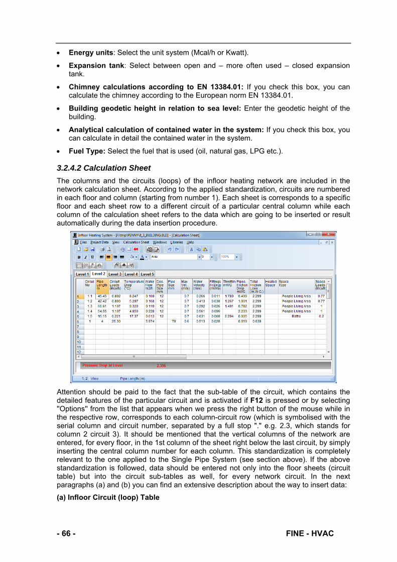
Energy units: Select the unit system (Mcal/h or Kwatt).

Expansion tank: Select between open and – more often used – closed expansion tank.

Chimney calculations according to EN 13384.01: If you check this box, you can calculate the chimney according to the European norm EN 13384.01.

Building geodetic height in relation to sea level: Enter the geodetic height of the building.

Analytical calculation of contained water in the system: If you check this box, you can calculate in detail the contained water in the system.

Fuel Type: Select the fuel that is used (oil, natural gas, LPG etc.).

3.2.4.2 Calculation Sheet

The columns and the circuits (loops) of the infloor heating network are included in the network calculation sheet. According to the applied standardization, circuits are numbered in each floor and column (starting from number 1). Each sheet is corresponds to a specific floor and each sheet row to a different circuit of a particular central column while each column of the calculation sheet refers to the data which are going to be inserted or result automatically during the data insertion procedure.

Attention should be paid to the fact that the sub-table of the circuit, which contains the detailed features of the particular circuit and is activated if F12 is pressed or by selecting ''Options'' from the list that appears when we press the right button of the mouse while in the respective row, corresponds to each column-circuit row (which is symbolised with the serial column and circuit number, separated by a full stop "." e.g. 2.3, which stands for column 2 circuit 3). It should be mentioned that the vertical columns of the network are entered, for every floor, in the 1st column of the sheet right below the last circuit, by simply inserting the central column number for each column. This standardization is completely relevant to the one applied to the Single Pipe System (see section above). If the above standardization is followed, data should be entered not only into the floor sheets (circuit table) but into the circuit sub-tables as well, for every network circuit. In the next paragraphs (a) and (b) you can find an extensive description about the way to insert data:

(a) Infloor Circuit (loop) Table

- 66 - FINE - HVAC

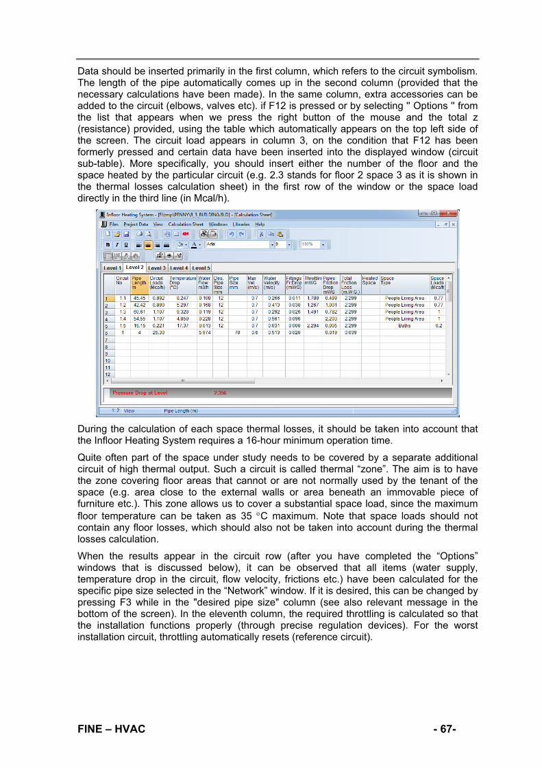
Data should be inserted primarily in the first column, which refers to the circuit symbolism. The length of the pipe automatically comes up in the second column (provided that the necessary calculations have been made). In the same column, extra accessories can be added to the circuit (elbows, valves etc). if F12 is pressed or by selecting '' Options '' from the list that appears when we press the right button of the mouse and the total z (resistance) provided, using the table which automatically appears on the top left side of the screen. The circuit load appears in column 3, on the condition that F12 has been formerly pressed and certain data have been inserted into the displayed window (circuit sub-table). More specifically, you should insert either the number of the floor and the space heated by the particular circuit (e.g. 2.3 stands for floor 2 space 3 as it is shown in the thermal losses calculation sheet) in the first row of the window or the space load directly in the third line (in Mcal/h).

During the calculation of each space thermal losses, it should be taken into account that the Infloor Heating System requires a 16-hour minimum operation time.

Quite often part of the space under study needs to be covered by a separate additional circuit of high thermal output. Such a circuit is called thermal “zone”. The aim is to have the zone covering floor areas that cannot or are not normally used by the tenant of the space (e.g. area close to the external walls or area beneath an immovable piece of furniture etc.). This zone allows us to cover a substantial space load, since the maximum floor temperature can be taken as 35 C maximum. Note that space loads should not contain any floor losses, which should also not be taken into account during the thermal losses calculation.

When the results appear in the circuit row (after you have completed the “Options” windows that is discussed below), it can be observed that all items (water supply, temperature drop in the circuit, flow velocity, frictions etc.) have been calculated for the specific pipe size selected in the “Network” window. If it is desired, this can be changed by pressing F3 while in the "desired pipe size" column (see also relevant message in the bottom of the screen). In the eleventh column, the required throttling is calculated so that the installation functions properly (through precise regulation devices). For the worst installation circuit, throttling automatically resets (reference circuit).

FINE – HVAC - 67-

(b) Options window (Circuit Sub-table)

As it has already been discussed above, control is transferred to the sub-table by pressing F12 or by selecting '' Options'' from the list that appears when we press the right button of the mouse in the relevant row of the circuit table.

Data appearing in the columns of this sub-table, as it can be seen, are as follows:

Heated space: The floor and space numbers are entered as they are appeared in the Thermal Losses calculation sheet (e.g. 1.2).

Space type: It is determined whether it is a people living area, a bath or a high thermal capacity area.

Space loads: It concerns the total space load, which automatically appears after selecting the "Heated space" or typing it directly.

Floor surface (m2): Insert the floor area of the heated space.

Space temperature (C): Enter the desired space temperature.

Under heated Space Room temperature (C): Enter the temperature of the space located under the heated space.

Coefficient of thermal resistance (Upward) (m²K/W): Enter the coefficient of upward thermal resistance either by typing it directly or by selecting it from the table that opens.

Coefficient of thermal Conduction (Downward) (W/m²K): Enter the coefficient of downward thermal resistance either by typing it directly or by selecting it from the table that opens.

Thermal flow density (Mcal/h/m²): When the above fields have been completed, the density of thermal flow is automatically calculated.

Mean floor temperature (C): When the above fields have been completed, the mean temperature of the floor surface is automatically calculated.

Max. floor temperature (C): The maximum allowable floor area temperature appears according to DIN 4725. Specifically, for residential areas tFBmax 29 C, for high thermal capacity area tFBmax 35 C and for baths tFB ti + 9 C, where ti is the space temperature.

Desired floor temperature (C): If the Mean floor surface temperature that has been calculated exceeds the Maximum floor surface temperature, enter a desired mean floor temperature so as to calculate the length of the pipes.

Corrected heat transfer density (Mcal/h/m²): The corrected value of the thermal flow thickness is then calculated and shown.

- 68 - FINE - HVAC

FINE – HVAC - 69-

Fall Short Thermal Power (Mcal/h): This result concerns the power that cannot be covered by the particular piping arrangement. Consequently, the designer should shorten the piping spacing RA, define a thermal zone or install a radiator.

Pipes spacing RA (cm): Enter the RA spacing of the pipes.

Mean water temperature (ºC): The average water temperature is calculated and shown.

Downward thermal flow density (KWatt/m²): The density of thermal flow downward appears, as calculated by the program.

Total Power of infloor system (Mcal/h): The total infloor heating power of the installation is calculated.

Circuit length (m): The required circuit length (net section) is calculated according to all the above mentioned data.

Supply and return circuit length (m): Insert the total inlet and return length from the vertical pipe to the circuit.

Sum of coefficients z of the additional accessory fittings: Enter the sum of the z coefficients of all the fittings that are used in this circuit.

Some of the above values should be typed while others are automatically calculated (the ones in red). Default values, which are the more common in each case, have been inserted in advance so that the user will not have to insert data in all fields.

Any modifications in the above data bring about correspondent modifications in the values of the circuit sheet, which instantly appear on the screen. In this way, the user supervises and controls the procedure fully.

Regarding the calculations, it should be clarified that the space type (residential area, bath or high thermal capacity area) automatically determines the maximum floor temperature (29, 33 or 35 respectively). If the mean floor surface temperature is higher than the maximum floor surface temperature, then the desired mean floor temperature should be inserted. In this case, the circuit will not cover all losses. For this reason, the remaining fall sort thermal power appears. Moreover, pipe spacing RA constitutes one of the principal parameters determined by the user in each space. If this spacing is shortened, the circuit pipe length is obviously increased and the mean water temperature drops. In all cases it is assumed that the circuit length should not exceed a certain limit which is set by the manufacturer of the particular pipe type and is approximately 150 m.

3.2.4.3 Calculation of other equipment

Other equipment, concerning mainly the heating engine room, is calculated through a series of windows, each one taking care of a specific part. Those windows for the infloor heating installation concern in particular the Boiler – Heat pump, the Burner, the Fuel Tank, the Circulator pump, the Expansion Tank, the Chimney and the Hot Water Storage Tank, as also explained for the single and two pipes heating system presented earlier.

3.2.4.4 Vertical Diagram

This option creates the vertical diagram of the network. The Boiler Room is located on the bottom side with its specific features automatically transferred from the calculation sheet.

3.2.4.5 Libraries

Infloor Heating System Libraries include pipes as well as boilers, heat pumps, burners, circulators and expansion tanks as in the case of Single and Two Pipes Systems.

3.3 Air-Conditioning The Air-conditioning package consists of four applications, which function either independently or in conjunction with each other. These applications are:

Cooling Loads: Cooling Loads are calculated (with the use of Ashrae or Carrier method) in each building floor and space, a procedure which usually comprises the first step of an Air-conditioning project.

Fan Coils: In this application all the necessary calculations for the installation of fan coils units are carried out and the required equipment is selected (pipes, cooling system, pump, safety device etc.).

Air Ducts: All the necessary calculations for the installation of a duct network are carried out (with one of the three known methods) and the required equipment is selected (duct dimensions, duct grills, fan etc.).

Psychrometrics: The air distribution in the air-conditioned spaces is estimated based on detailed psychometric equations, the psychometric change is depicted on the Psychometric Chart and the appropriate air-conditioning unit is selected.

FINE – HVAC - 71-

3.3.1 Cooling Loads When the program is loaded, the main menu with the option groups "Files", "Project Data", "Windows", "Libraries" and "Help" appears on the screen. “Project Data” are divided in project info (headings of the project), indoor design conditions, building parameters, climatological data, months, structural elements, people, equipment and lighting loads.

3.3.1.1 Indoor design conditions

You define the desired indoor humidity (desired relative % humidity in the air-conditioned spaces) and temperature (desired temperature in °C in the air-conditioned spaces) along with the temperature difference between outdoor and non air-conditioned spaces (in °C) and the temperature difference between soil and air-conditioned spaces (in °C).

3.3.1.2 Building Parameters

The data of the respective window include the following:

Area with Fog: In case there is usually fog in the area, check this box.

Number of levels (floors): The levels of the building can be up to 15.

Default Height (m): This value will automatically update the height of the walls in the calculation sheet, while you will be able to make modifications wherever you desire.

Energy units: You select the units of the project (Mcal/h, KWatt, KBtu/h).

Resistance coefficient unit system: You select the units of the resistance coefficients (Kcal/hm²C or Watt/m²K).

Calculation method: The program gives the option to select among Carrier, ASHRAE CLTD, ASHRAE TFM, ASHRAE RTS 2001 or 2013 and ASHRAE Ships (Merchant or Naval) calculation methods. Moreover, when you complete the data entry procedure with one of these methods, you can compare the results with those of another method, by simply altering it.

Safety Factor (%): You can define in any desired space a general increase factor for the loads (e.g. 5%), which will increase accordingly all the individual loads of the space.

Opening hour – Closing hour (1-24): Through these two options you can determine the range of the time period in which you wish to have the calculation results (e.g. initial time 8 until final time 18). Naturally, the selection can be made for the whole 24 hours’ time (from 1 o’clock until 24 o’clock) but the result volume will be larger.

Rotation angle: If you want to change the orientation of the building, you can rotate it to a specific angle through selecting it from the list.

Vessel type: If the ASHRAE Ships method has been chosen, select the type of the vessel.

3.3.1.3 Climatological Data

The data refer to the selected city, displaying the corresponding climatologic data (latitude, longitude, altitude, mean maximum temperatures, corresponding daily ranges for 6 months etc.) as well as the average relative humidity in summer.

3.3.1.4 Months

The Reference month and Calculation months (i.e. from April until September) are defined in this window.

- 72 - FINE - HVAC

3.3.1.5 Structural Elements

This term corresponds to some common element types which characterise the building and more specifically the typical structural elements such as outer and inner walls, ceilings, floors and openings.

Outer walls are specified through their U factor coefficient, weight (100, 300, 500, 700 kg), colour (light, intermediate, dark), as well as standardisation by ASHRAE method (A, B, C, D, Ε, F, G). You can select the desired typical data from the relevant library.

Ceilings are specified through their U factor coefficient, weight (50, 100, 200, 300 kg), colour (light, intermediate, dark), and type by Carrier (sunny, shady, under water or watered) or by ASHRAE (types 1, 2, 3... 11 with or without suspended ceiling).

Inner walls and floors are specified through their U factor coefficient.

Openings are specified through their dimensions (in m), U factor coefficient, glass coefficient, frame type, coefficient of air penetration a (the same coefficient applied in heating) and glazing system. As far as the glass coefficient is concerned, a detailed auxiliary table is available.

FINE – HVAC - 73-

3.3.1.6 People

In case you want to define the same people loads for all the spaces, you complete the following window.

You select a description from the list that appears by pressing F11 or right click of the mouse and automatically the sensible, the latent load and the radiant heat are completed. The only thing that you have to do is enter the quantity in the last column which will be either the number of persons in the space per m² or the number of persons in the space (depending on which option you will check). Furthermore, you can select the operating schedule depending on the building type by pressing the selection button.

When this window is filled in, all the spaces in the calculation sheet will automatically get the same people loads but you can modify them separately in each space inside the calculation sheet.

- 74 - FINE - HVAC

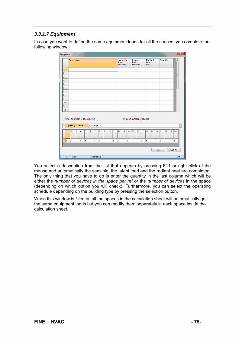
3.3.1.7 Equipment

In case you want to define the same equipment loads for all the spaces, you complete the following window.

You select a description from the list that appears by pressing F11 or right click of the mouse and automatically the sensible, the latent load and the radiant heat are completed. The only thing that you have to do is enter the quantity in the last column which will be either the number of devices in the space per m² or the number of devices in the space (depending on which option you will check). Furthermore, you can select the operating schedule depending on the building type by pressing the selection button.

When this window is filled in, all the spaces in the calculation sheet will automatically get the same equipment loads but you can modify them separately in each space inside the calculation sheet.

FINE – HVAC - 75-

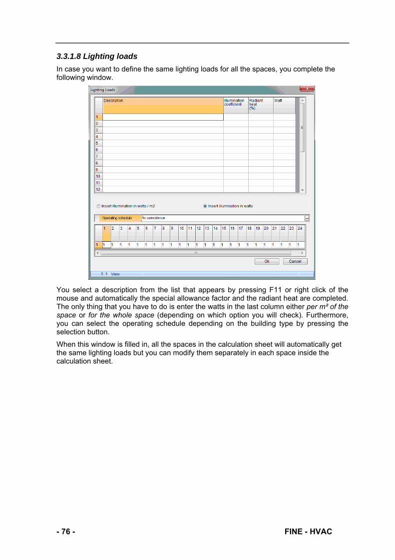
3.3.1.8 Lighting loads

In case you want to define the same lighting loads for all the spaces, you complete the following window.

You select a description from the list that appears by pressing F11 or right click of the mouse and automatically the special allowance factor and the radiant heat are completed. The only thing that you have to do is enter the watts in the last column either per m² of the space or for the whole space (depending on which option you will check). Furthermore, you can select the operating schedule depending on the building type by pressing the selection button.

When this window is filled in, all the spaces in the calculation sheet will automatically get the same lighting loads but you can modify them separately in each space inside the calculation sheet.

- 76 - FINE - HVAC

3.3.1.9 Calculation Sheet

The calculation sheets for the space loads are included in the respective building floor sheets. If one of the floors is selected, a list will appear containing the respective load sheets for the floor spaces. The functionality is quite similar to the one described for the heating losses spaces.

The screen that corresponds to the space data is divided in two parts: the upper part refers to the loads due to the structural elements of the space, while the lower part refers to the additional loads due to lighting, people, equipment etc.

Concerning the upper part of the screen, each row refers to a specific typical structural element (e.g. W1, O1 etc.). The data inserted (either from you or automatically through the drawings) correspond to the Orientation, the Length (m) and Height (m) of the building element, as well as the number of equal surfaces if exist. Openings are subtracted automatically from walls, if orientations are alike.

When the “ASHRAE Ships” method is selected, the extra column “Adjoining space” has to be filled in.

Optionally, in the last three columns, the data for the shading calculation can be typed. Three different shading mechanisms are possible:

Inside shading: This applies only to windows in the case there are blinds, roller shades etc. that cover their total surface at the same time. The most common values for each case and according to the glass type appear in the auxiliary table, which is activated when F11 or the selection button of the field is pressed.

Projection shading: This applies mainly to openings but it can be also used for wall surfaces. If you press the right button of the mouse while in the respective column and row and select from the list ''Options'', the window of the adjacent figure appears in the right corner of the screen. Here you can fill the width of the horizontal and (or) vertical projection of the opening and its distance from it. For example, for a balcony of one-meter width, which hangs 0.5 meter above the O1 window, you type ‘’1’’ in the field of the horizontal projection width and ‘’0.5’’ in the field of the horizontal projection

FINE – HVAC - 77-

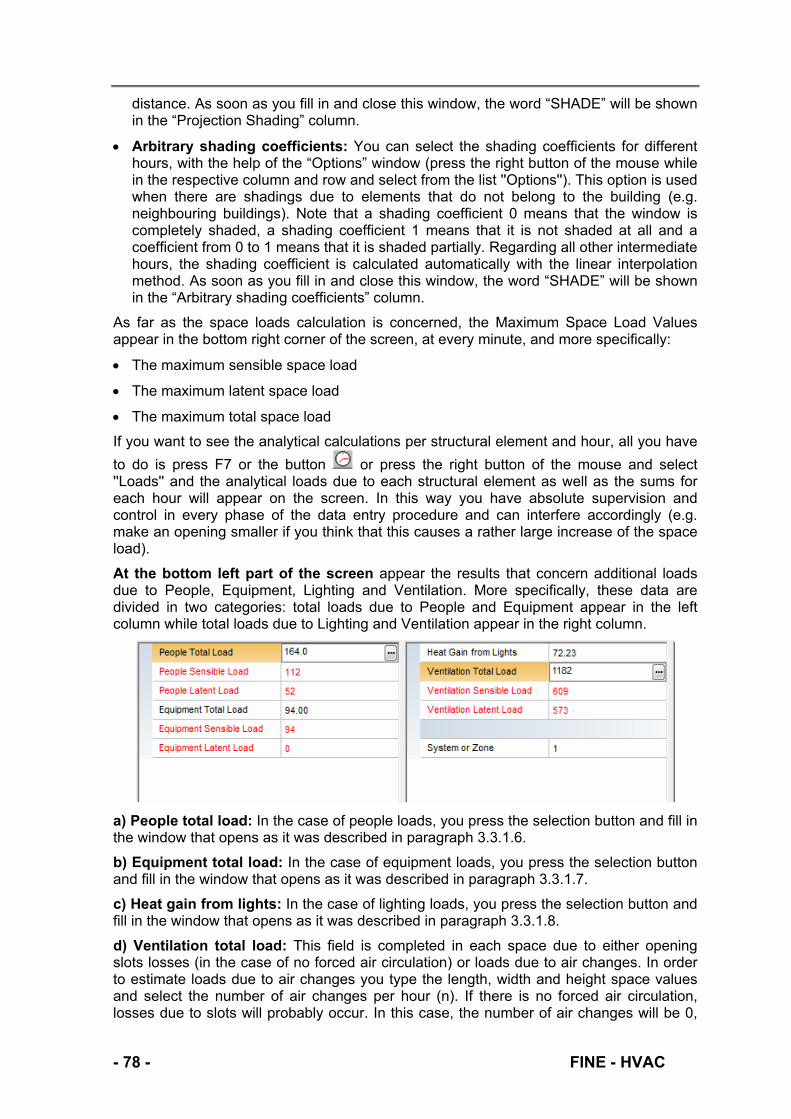
distance. As soon as you fill in and close this window, the word “SHADE” will be shown in the “Projection Shading” column.

Arbitrary shading coefficients: You can select the shading coefficients for different hours, with the help of the “Options” window (press the right button of the mouse while in the respective column and row and select from the list ''Options''). This option is used when there are shadings due to elements that do not belong to the building (e.g. neighbouring buildings). Note that a shading coefficient 0 means that the window is completely shaded, a shading coefficient 1 means that it is not shaded at all and a coefficient from 0 to 1 means that it is shaded partially. Regarding all other intermediate hours, the shading coefficient is calculated automatically with the linear interpolation method. As soon as you fill in and close this window, the word “SHADE” will be shown in the “Arbitrary shading coefficients” column.

As far as the space loads calculation is concerned, the Maximum Space Load Values appear in the bottom right corner of the screen, at every minute, and more specifically:

The maximum sensible space load

The maximum latent space load

The maximum total space load

If you want to see the analytical calculations per structural element and hour, all you have

to do is press F7 or the button or press the right button of the mouse and select ''Loads'' and the analytical loads due to each structural element as well as the sums for each hour will appear on the screen. In this way you have absolute supervision and control in every phase of the data entry procedure and can interfere accordingly (e.g. make an opening smaller if you think that this causes a rather large increase of the space load).

At the bottom left part of the screen appear the results that concern additional loads due to People, Equipment, Lighting and Ventilation. More specifically, these data are divided in two categories: total loads due to People and Equipment appear in the left column while total loads due to Lighting and Ventilation appear in the right column.

a) People total load: In the case of people loads, you press the selection button and fill in the window that opens as it was described in paragraph 3.3.1.6.

b) Equipment total load: In the case of equipment loads, you press the selection button and fill in the window that opens as it was described in paragraph 3.3.1.7.

c) Heat gain from lights: In the case of lighting loads, you press the selection button and fill in the window that opens as it was described in paragraph 3.3.1.8.

d) Ventilation total load: This field is completed in each space due to either opening slots losses (in the case of no forced air circulation) or loads due to air changes. In order to estimate loads due to air changes you type the length, width and height space values and select the number of air changes per hour (n). If there is no forced air circulation, losses due to slots will probably occur. In this case, the number of air changes will be 0,

- 78 - FINE - HVAC

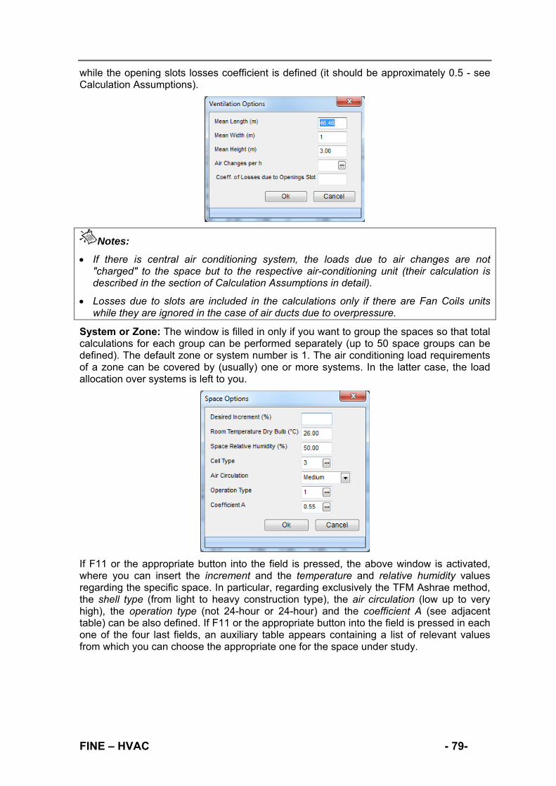
while the opening slots losses coefficient is defined (it should be approximately 0.5 - see Calculation Assumptions).

Notes:

If there is central air conditioning system, the loads due to air changes are not "charged" to the space but to the respective air-conditioning unit (their calculation is described in the section of Calculation Assumptions in detail).

Losses due to slots are included in the calculations only if there are Fan Coils units while they are ignored in the case of air ducts due to overpressure.

System or Zone: The window is filled in only if you want to group the spaces so that total calculations for each group can be performed separately (up to 50 space groups can be defined). The default zone or system number is 1. The air conditioning load requirements of a zone can be covered by (usually) one or more systems. In the latter case, the load allocation over systems is left to you.

If F11 or the appropriate button into the field is pressed, the above window is activated, where you can insert the increment and the temperature and relative humidity values regarding the specific space. In particular, regarding exclusively the TFM Ashrae method, the shell type (from light to heavy construction type), the air circulation (low up to very high), the operation type (not 24-hour or 24-hour) and the coefficient A (see adjacent table) can be also defined. If F11 or the appropriate button into the field is pressed in each one of the four last fields, an auxiliary table appears containing a list of relevant values from which you can choose the appropriate one for the space under study.

FINE – HVAC - 79-

When the “ASHRAE RTS 2013” method has been selected, the extra options “Roof load absorbed in the return air-stream” and “Lighting load absorbed in the return air-stream” appear.

The sensible load part of all the above additional loads is added to the total load of the structural elements and the final sum corresponds to the total room sensible load.

If the latent loads due to people and equipment are summed up, the total space latent load results. The total sensible plus the total latent load comprise the total space load. These per hour values are shown in the calculation sheet mentioned above.

In order to insert data faster, in case they have to be analytically typed (that is, if they are not automatically updated from drawings through FINE HVAC), the program enables you to copy a typical floor (extremely usual in practice) and a typical space, as shown in the heating losses application.

3.3.1.10 Temperatures

The results of this window are directly linked to the applied method, which means that some intermediate results-admissions of the methodology are shown.

3.3.1.11 Building Loads Summary

The total building loads are shown for each month and hour without including ventilation.

- 80 - FINE - HVAC

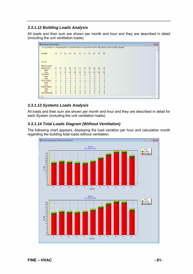
3.3.1.12 Building Loads Analysis

All loads and their sum are shown per month and hour and they are described in detail (including the unit ventilation loads).

3.3.1.13 Systems Loads Analysis

All loads and their sum are shown per month and hour and they are described in detail for each System (including the unit ventilation loads).

3.3.1.14 Total Loads Diagram (Without Ventilation)

The following chart appears, displaying the load variation per hour and calculation month regarding the building total loads without ventilation.

FINE – HVAC - 81-

3.3.1.15 Total Loads Diagram (With Ventilation)

The above chart appears, displaying the load variation per hour and calculation month regarding the building total loads including ventilation.

3.3.1.16 Systems Diagram

The following chart appears, displaying the load variation per hour and calculation month regarding the total loads for each system.

3.3.1.17 Libraries

Libraries refer to structural element types (walls, openings, ceilings etc.), temperature data as well as auxiliary loads and their coincidences (people, equipment etc.).

- 82 - FINE - HVAC

You can insert and use your own data, easily by selecting a category (e.g. the external

walls as it is shown above) and press the append record button . In the new line you fill

in the element data, press to save them and OK to close the window.

FINE – HVAC - 83-

3.3.2 Fan Coils The main menu of the Fan Coils application includes the options "Files”, “Project Data”, “View”, “Windows”, “Libraries” and “Help”. “Files”, “View” and “Help” are similar to the “Two pipes heating system” application and are discussed in detail in paragraphs 3.1.1, 3.1.3 and 3.1.6 respectively. The rest are described in short in the following paragraphs.

3.3.2.1 Project Data

This pertains to the project basic data, which are divided into Project info (project headings) and Network data. Network data include:

Water temperature (ºC): Enter the inlet water temperature in C (the return temperature is calculated automatically)

FCUs Temperature Difference (ºC): Enter the fan coils units temperature difference (usual value Dt=5 C)

Dry bulb temperature (ºC): Enter the dry bulb room temperature.

Wet bulb temperature (ºC): Enter the wet bulb room temperature.

Main pipe type: Select the type of the main pipes (e.g. steel pipes).

Main pipes roughness factor: The roughness factor is entered automatically, depending on the pipe type you have selected but if you want, you can modify it. The measurement unit used by the program is μm.

Secondary pipe type: Select the type of the secondary pipes (in case two types are used).

Secondary pipes roughness factor: The roughness factor is entered automatically, depending on the pipe type you have selected but if you want, you can modify it. The measurement unit used by the program is μm.

Maximum water velocity (m/s): Enter the maximum desired water velocity limit (based on which the cross-sections are calculated).

Friction limit per meter length of piping (mwg/m): Enter the friction limit per length of the piping. The recommended maximum pressure drop in water supply systems is 30 kPa per 30 m of equivalent pipe length, i.e. 10% approximately, or 10 m of water column per 100 m of equivalent pipe length.

Number of pumps: In case you have more than one pump, enter their number here so as to be able to use them in the Calculation sheet and the Circulator calculation.

Energy units: Select the unit system.

Type of cooling engine: You can select between an air cooled or a water cooled engine.

FCU model: By pressing the selection button, you choose from the library the type of the FCUs. If you want, you can add your own suppliers and units in the Libraries -> FCUs.

Temperature variation per meter length of piping (ºC/m): If the pipes are not well insulated, enter the temperature variation per meter. In case they are insulated, this value is zero.

FCU fan speed: Select from the list the speed of the fan among low, medium or high.

FINE – HVAC - 85-

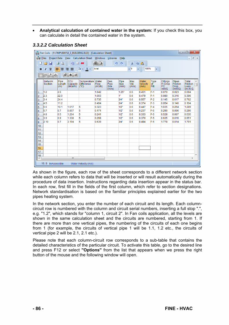
Analytical calculation of contained water in the system: If you check this box, you can calculate in detail the contained water in the system.

3.3.2.2 Calculation Sheet

As shown in the figure, each row of the sheet corresponds to a different network section while each column refers to data that will be inserted or will result automatically during the procedure of data insertion. Instructions regarding data insertion appear in the status bar. In each row, first fill in the fields of the first column, which refer to section designations. Network standardisation is based on the familiar principles explained earlier for the two pipes heating system.

In the network section, you enter the number of each circuit and its length. Each column-circuit row is numbered with the column and circuit serial numbers, inserting a full stop ".", e.g. "1.2", which stands for "column 1, circuit 2". In Fan coils application, all the levels are shown in the same calculation sheet and the circuits are numbered, starting from 1. If there are more than one vertical pipes, the numbering of the circuits of each one begins from 1 (for example, the circuits of vertical pipe 1 will be 1.1, 1.2 etc., the circuits of vertical pipe 2 will be 2.1, 2.1 etc.).

Please note that each column-circuit row corresponds to a sub-table that contains the detailed characteristics of the particular circuit. To activate this table, go to the desired line and press F12 or select ''Options'' from the list that appears when we press the right button of the mouse and the following window will open.

- 86 - FINE - HVAC

In the above window, the cells “Conditioned space”, “Space sensible heat” and “Space latent heat” will be automatically inserted if from the application of Cooling Loads you have previously exported the results to the Fan coils application (in the Cooling Loads window, from Files menu choose Export to -> Fan coils) otherwise, you can add them on your own and automatically the fan coil type will be selected.

If there are more than one Fan Coil unit in the same space, you must intervene by allocating the load accordingly. Calculation of the fan coil unit is performed automatically in relation to the information of the network data and displayed in the above window.

Regarding fittings, friction drops, similar sections, Reverse Return type of networks etc., same rules as stated earlier for two pipes heating system, can be applied.

3.3.2.3 Cooling Engine

In this window a Cooling engine or a Cooling tower is selected (from Libraries, if F11 or the appropriate button into the field is pressed) and its operation features are inserted. Note that detailed calculations for the cooling system are performed within the Psychrometrics application.

“Network Drawing”, “Vertical Diagram”, “Sections friction drop” options, as well as the windows “Technical Description”, “Assumptions” “Bill of materials” and “Cover Page” follow the rules stated in the previous paragraphs.

3.3.2.4 Libraries

The "Fan Coils" application libraries contain pipes, FC units and fittings as well as equipment for the engine-room (Cooling engines, Pumps, Expansion Tanks etc). Each library category contains various material types, which exist in the market, but it can be easily updated with the material types you want. As far as the "Fan Coils" library is concerned, various unit types are registered. Specifically, for each manufacturer a tab is displayed with fan coil sizes (200, 400 etc.), Z coefficients, codes and costs.

If the key “Loads” is pressed, the corresponding outputs for the various temperatures (dry bulb, wet bulb and water inlet temperature) are displayed.

FINE – HVAC - 87-

You can insert and use your own data, easily by selecting a category (e.g. pipes as it is

shown below) and press the append record button . In the new line you fill in the pipe

data (inserting and the Diameters), press to save them and OK to close the window.

- 88 - FINE - HVAC

3.3.3 Air-Ducts When the program is loaded, the main menu with the option groups "Files", "Project Data", "Windows", "Libraries" and "Help" appears on the screen. “Files”, “View”, most “Windows” options and “Help” are similar to what has been described earlier (paragraphs 3.1.1, 3.1.3 and 3.1.6 respectively), while the rest are summarized below. These options and their secondary options are described in detail in the following paragraphs.

3.3.3.1 Project Data

This pertains to the project basic data, which are divided into Project info (project headings) and Network data. Network data include:

Air Supply temperature (ºC): In this field you fill in the temperature of the air entering the space from the supply grilles (15-16C).

Desired Spaces temperature (ºC): This is the desired temperature in the air-conditioned spaces (significant only if Psychrometrics has not been preceded).

Air-duct material: The Air-duct material to be used is selected (if F11 or the appropriate button into the field is pressed, the respective library is displayed).

Air-Ducts Roughness Factor (μm): Air-duct roughness factor which depends on the duct material is inserted. If the duct material has been selected from the libraries, roughness is automatically updated.

Secondary air-duct material: The secondary air-duct material to be used is selected (if F11 or the appropriate button into the field is pressed, the respective library is displayed).

Secondary air-ducts Roughness Factor (μm): Air-duct roughness factor, which depends on the secondary duct material, is inserted. If the duct material has been selected from the libraries, roughness is automatically updated.

Maximum air velocity (m/s): This field concerns the upper air velocity limit in the air ducts. This value is used as an upper limit if the method of equal pressure drops is applied or it is taken as the value of the air velocity when the method of equal velocities is applied instead.

Pressure drop per meter (mm. W.G./m): This is the value of the corresponding network pressure drop per m when the equal friction method is applied, while it is of no significance if the method of velocity reduction is applied instead.

Type of Cross-Section: Cross section type in the longest part of the network is inserted (circular, square or rectangular). Of course, there is always the possibility to modify it in a specific section of the network.

Desired Air-duct dimensions (width and height): The desired air duct dimensions should be determined only if rectangular air ducts are selected where you are able to define a fixed value for width or height. Note that, when both dimensions of the air-duct rectangular cross section are determined (or one dimension for circular or square cross sections), then the velocity and pressure drop in each network branch are determined without following the principles of any of the available methods. On the contrary, if only one dimension is inserted, height or width, then the other dimension results automatically from the selected calculation method. Of course, the fixed value for height or width determined here, does not constrain you because there is always the possibility to modify it in a specific section of the network.

FINE – HVAC - 89-

Rounding step of Air-duct dimensions (mm): In case that accuracy to mm is not needed, the air-duct cross-section value is calculated approximately in increments (e.g. 50 mm).

Grilles Sound Level (dB): This field concerns the upper limit of the noise level at grilles, which should not be exceeded. This limit can also be selectively modified for a specific room grille.

Desired grilles dimensions (length and width): Similar instructions to those given above for the desired air duct dimensions are applied.

Number of Fans: It concerns the number of the installation Fans (1-40).

Energy units: Υοu can choose the units of the results among Mcal/h, KWatt or KBtu/h.

Calculation Method: You can select the calculation method among the three available, a) Velocity reduction b) Equal friction and c) Static regain.

Minimum Air velocity (Regain method): This concerns the minimum air velocity in case the Static regain method is selected. You should keep in mind that you are allowed to insert a minimum velocity limit value, if the velocity at the air outlets is considered very low.

Speed calculation method: You can select the speed calculation method between the one with Equivalent cross section area or with Real duct cross section area.

3.3.3.2 Calculation Sheet

As shown in the figure, each row of this sheet corresponds to a different network section while each column refers to data concerning this network section (see status bar). The operation concepts are based on the principles stated earlier. The starting point of the air-duct network (where the fan is located) corresponds to the number 1. The total air flow rate in each space can be calculated either approximately based on the Space load and the Temperature difference between supply and return air or accurately if Psychrometric Calculations have been previously performed (see Psychrometrics application). Given the values of those data, flow rate values are summed up properly and are automatically displayed in the Air flow column. Based on these flow rates in each network section and the calculation method (equal pressure or velocity), air-duct dimensions as well as standard sizes for the grilles are determined in each section. Air-duct cross section

- 90 - FINE - HVAC

(circular, rectangle etc.) and its desired dimensions are those entered in the general data, but you modify or insert any other desired dimension here.

Based on the above dimensions, effective air velocity and pressure drop can be calculated in the calculation sheet.

Finally, the respective grille dimensions are also determined so that the noise level, specified in general data, is not exceeded. The grille dimensions are automatically calculated after a grille type has been selected on Network window from the respective library by pressing F11 or the appropriate button into the field, as it is shown below.

The grille width, height and existing noise level are displayed at the bottom of the calculation sheet window. Note that in the middle of the window, it is possible to insert the desired dimensions (usually one of them is inserted in the general data and the other one is automatically calculated).

Fittings of the air-duct network (e.g. elbows, T-junctions etc.) are entered for each section in the column “Type of fittings” by activating the corresponding window with F11 or the appropriate button into the field.

Note that, in case the equal friction method is used and you want to balance the network, dampers can be adjusted accordingly (keep in mind that the equal pressures method ensures well "balanced" networks only if the network has been symmetrically designed). The column “Air ducts Friction Drop” shows how well balanced the network is and indicates which sections need restriction using dampers.

If the method of static regain is applied instead, then friction losses in each network section are balanced by the recovered static pressure, which in turn depends on the velocity in the previous and next section. So, nothing appears in “Total friction loss” column (zero friction losses), except for the first network section that starts at the fan (section 1.2 in the above example) and, of course, the sections where you have specified both dimensions of the air-duct cross section. Consequently, total friction losses in this case are equal to the friction losses in the first section, which starts at the fan.

FINE – HVAC - 91-

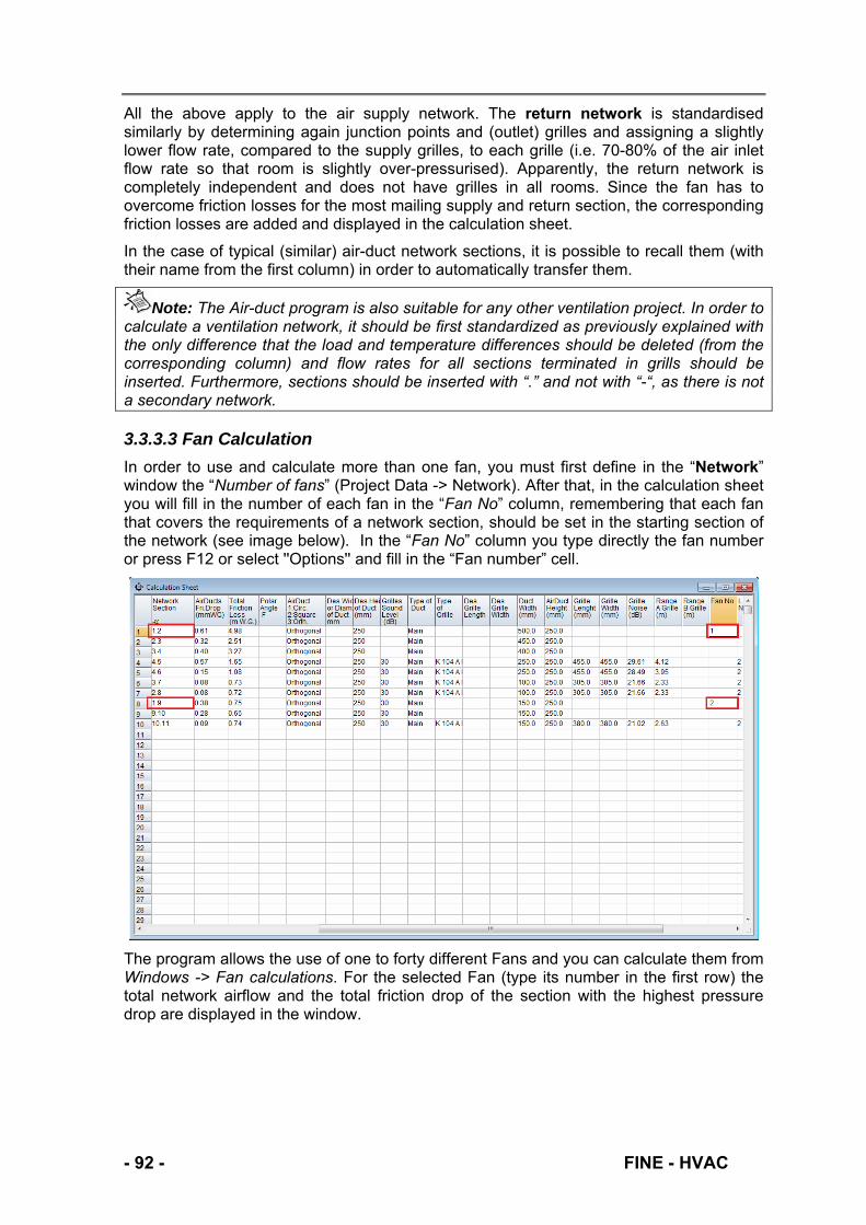
All the above apply to the air supply network. The return network is standardised similarly by determining again junction points and (outlet) grilles and assigning a slightly lower flow rate, compared to the supply grilles, to each grille (i.e. 70-80% of the air inlet flow rate so that room is slightly over-pressurised). Apparently, the return network is completely independent and does not have grilles in all rooms. Since the fan has to overcome friction losses for the most mailing supply and return section, the corresponding friction losses are added and displayed in the calculation sheet.

In the case of typical (similar) air-duct network sections, it is possible to recall them (with their name from the first column) in order to automatically transfer them.

Note: The Air-duct program is also suitable for any other ventilation project. In order to calculate a ventilation network, it should be first standardized as previously explained with the only difference that the load and temperature differences should be deleted (from the corresponding column) and flow rates for all sections terminated in grills should be inserted. Furthermore, sections should be inserted with “.” and not with “-“, as there is not a secondary network.

3.3.3.3 Fan Calculation

In order to use and calculate more than one fan, you must first define in the “Network” window the “Number of fans” (Project Data -> Network). After that, in the calculation sheet you will fill in the number of each fan in the “Fan No” column, remembering that each fan that covers the requirements of a network section, should be set in the starting section of the network (see image below). In the “Fan No” column you type directly the fan number or press F12 or select ''Options'' and fill in the “Fan number” cell.

The program allows the use of one to forty different Fans and you can calculate them from Windows -> Fan calculations. For the selected Fan (type its number in the first row) the total network airflow and the total friction drop of the section with the highest pressure drop are displayed in the window.

- 92 - FINE - HVAC

Regarding the selected Fan number (1, if only one fan exists), the following data appear:

The calculated air flow in m3/h, according to the calculation sheet data.

The highest pressure drop section (in mmWG), that is the section with the highest friction losses.

The total Network (pipes and fittings) Friction Drop, which corresponds to the above section and has been calculated in calculation sheet.

The filters, alternator air-air and air-conditioning unit friction drops as well as other friction losses (for safety reasons, some further friction losses are supposed, that is the theoretically calculated friction values are usually increased by approximately 20-30%, in mmWG).

If the above friction values are added together, the result will be the installation total Static pressure (in mmWG). In order to select a fan type from the program libraries, press F11 or the appropriate button into the field "Type of Selected Fan".

When you select the fan type, the following options will be completed automatically and you fill in only the Cost.

3.3.3.4 Libraries

The "Air-ducts" application libraries include duct materials, grilles, fittings and fans as well as the common Offer libraries. As in any other application, each library category contains various material types, which exist in the market, but naturally it can be updated with the material types you want. Fittings libraries contain the various air-duct fittings in list form while the main features of each fitting [Z coefficient (resistance) and cost] are also mentioned. Duct material library contains different types of materials (e.g. from Tin Plate, Plastic, etc.), along with their roughness and specific gravity and thickness. As for the "Grilles" library, it contains grille types with their standard dimensions and all other features needed for the calculations. You can insert and use your own data, easily by selecting a category (e.g. grilles as it is shown below) and press the append record

button . In the new line you fill in the grille data (inserting and the Size), press to save them and OK to close the window.

FINE – HVAC - 93-

- 94 - FINE - HVAC

3.3.4 Psychrometrics Based on the analytical psychrometric equations, this program carries out the air-conditioning unit selection and the air distribution in the air-conditioned spaces while it also provides the psychrometric variation on the psychrometric chart as a result. When the program is loaded, the main menu with the option groups "Files", "Project Data", “View”, "Windows" and "Help" appears on the screen. “Files”, “View”, “Help” and most of the “Windows” options are quite similar to the “Heating losses” application and are discussed in detail in paragraphs 3.1.1, 3.1.3 and 3.1.6 respectively. The rest are summarized in the following paragraphs.

3.3.4.1 Project Data

These are the basic data of the installation. They are divided into Project info (headings of the project), Calculation parameters, Indoor and Outdoor design conditions and, finally, Spaces data.

1) Calculation Parameters concern the following:

Minimum temperature of the psychrometric chart: Define the minimum temperature (°C), which will be shown in the psychrometric chart.

Maximum temperature of the psychrometric chart: Define the maximum temperature (°C), which will be shown in the psychrometric chart.

Energy units: You can select among Mcal/h, KWatt or KBtu/h units.

Outside air: The required outside air can be inserted either as a volume (in m3/h) or as a percentage of the total air (%).

Heat recovery unit: If a heat recovery unit is used, you select its type (Heat Recovery Ventilator or Energy Recovery Ventilator) otherwise you choose “No”.

Air-duct losses: Check this box if you want to take into account air duct losses, otherwise, they will be ignored.

Fan losses: You select ''No'' if you want the fan losses to be ignored, or choose between ‘‘Before’’ if the fan is located upstream of the air-conditioning unit, or ''After'' if the fan is located downstream of the air-conditioning unit.

By-pass factor BF: This concerns the air-conditioning unit by-pass factor and varies between 0 – 1 (0 means no by-pass at all, 1 means 100% by-pass).

Coolant temperature difference: Fill in the temperature difference of the coolant medium (°C).

Heating medium temperature difference: Fill in the temperature difference of heating medium (°C).

Outside air percentage: In case you have required the outside air to be inserted as a percentage, fill it in, in this field.

Air duct losses in percentage of room loads (%): In case you have checked the “Air duct losses” box, define them here as a percentage of the room loads.

Fan losses: In case you take into account the fan losses, you can define the load here (if you want, you can modify it in the “Systems” window later, selecting the specific system). The energy units are those that have been selected in “Energy units” field.

Percentage of supply air exhausted from space (%): In this field, you fill in the percentage of the supply air that is exhausted from the space.

FINE – HVAC - 95-

Altitude: Fill in the altitude of the location in m.

Outside air preheating: If a preheater is used in the heating system, select “Yes” in this field (you can also select or change it later in the “Systems” window).

Exit air temperature from preheater: In this field fill in the temperature of the air that is leaving the heater (you can also select or change it later in the “Systems” window).

2) Indoor design conditions concern the following:

Desired indoor temperature in summer: This concerns the desired temperature (in C) of the cooled rooms.

Desired indoor relative humidity in summer: This concerns the desired relative humidity (%) of the cooled rooms.

Desired indoor temperature in winter: This concerns the desired temperature (in C) of the heated rooms.

Desired indoor relative humidity in winter: This concerns the desired relative humidity (%) of the heated rooms.

3) Outdoor design conditions concern the outdoor temperature and relative humidity values during the day in summer as well as in winter.

4) Spaces

The data that will be used for the calculation of the air-conditioning units for each space should be typed in this window.

More specifically, for each space the following data should be typed:

The level where the space is, its number and name.

The system where the space belongs.

- 96 - FINE - HVAC

The hour when the maximum load appears, regarding the system where the space belongs.

The sensible (RSH) and latent (RLH) cooling load of the space.

The thermal losses of the space (WRSH).

The required outside air quantity of the space (VA).

The above data will be automatically completed as long as you have followed the following procedure:

1) For the cooling loads and the quantity of fresh air to be transferred:

- From the Cooling loads application, in the Calculation Sheet you fill in the “System or Zone” for each space (in case you have more than one system).

- When you finish, you select from Files -> Export to -> Systems - Psychrometry (total, spaces of ventilation loads)

- Open the Psychrometrics application and select Files -> Import from -> Cooling

2) For the thermal loads to be transferred:

- When you finish the Thermal losses application, select Files -> Export to -> Systems - Psychrometry

- Open the Psychrometrics application and select Files -> Import from -> Heating

3.3.4.2 Psychrometric Point Calculations

If this option is selected from the “Windows” menu, the basic psychrometric calculations are performed. In the following image if you provide two of the six basic psychrometric

quantities and press F8 or the calculation button from the toolbar, the remaining four quantities will be calculated.

FINE – HVAC - 97-

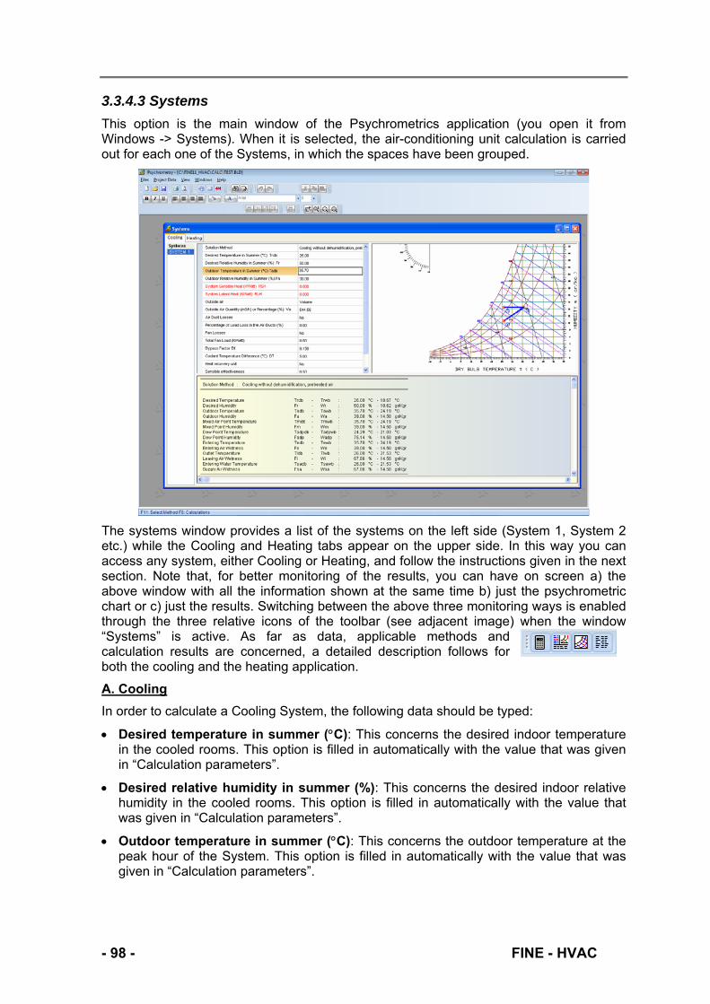
3.3.4.3 Systems

This option is the main window of the Psychrometrics application (you open it from Windows -> Systems). When it is selected, the air-conditioning unit calculation is carried out for each one of the Systems, in which the spaces have been grouped.

The systems window provides a list of the systems on the left side (System 1, System 2 etc.) while the Cooling and Heating tabs appear on the upper side. In this way you can access any system, either Cooling or Heating, and follow the instructions given in the next section. Note that, for better monitoring of the results, you can have on screen a) the above window with all the information shown at the same time b) just the psychrometric chart or c) just the results. Switching between the above three monitoring ways is enabled through the three relative icons of the toolbar (see adjacent image) when the window “Systems” is active. As far as data, applicable methods and calculation results are concerned, a detailed description follows for both the cooling and the heating application.

A. Cooling

In order to calculate a Cooling System, the following data should be typed:

Desired temperature in summer (C): This concerns the desired indoor temperature in the cooled rooms. This option is filled in automatically with the value that was given in “Calculation parameters”.

Desired relative humidity in summer (%): This concerns the desired indoor relative humidity in the cooled rooms. This option is filled in automatically with the value that was given in “Calculation parameters”.

Outdoor temperature in summer (C): This concerns the outdoor temperature at the peak hour of the System. This option is filled in automatically with the value that was given in “Calculation parameters”.

- 98 - FINE - HVAC

Outdoor relative humidity in summer (%): This concerns the relative humidity at the peak hour of the System. This option is filled in automatically with the value that was given in “Calculation parameters”.

System Sensible Heat: This is the sensible cooling load of the System at its peak hour. It is completed automatically from the sum of the sensible load RSH of each space of the system (from “Project Data” -> “Spaces”).

System Latent Heat: This concerns the latent cooling load of the System at its peak hour. It is completed automatically from the sum of the latent load RLH of each space of the system (from “Project Data” -> “Spaces”).

Outside air: The required outside air can be provided either as quantity in m3/h or as percentage. This option is filled in automatically with the value that was given in “Calculation parameters”.

Outside air quantity (m³/h) or percentage: This concerns the total outside air of the System in m³/h or the respective percentage. It is completed automatically from the sum of the air capacity VA of each space of the system (from “Project Data” -> “Spaces”).

Air-duct losses: You enter either ''No'' if you want to ignore the air duct losses, or ''Yes'' if you want them to be taken into account in the calculations. This option is filled in automatically with the value that was given in “Calculation parameters”.

Percentage of load loss in the air-ducts: In case you have selected “Yes” in the “Air duct losses” box, define here the percentage of the system loads. This option is filled in automatically with the value that was given in “Calculation parameters”.

Fan losses: In case you take into account the fan losses, you can define the load here. This option is filled in automatically with the value that was given in “Calculation parameters”.

Total fan load: To be inserted only if the fan load is to be taken into account in the calculations. This option is filled in automatically with the value that was given in “Calculation parameters”.

Bypass factor BF: This concerns the air-conditioning unit by-pass factor which varies between 0 - 1. This option is filled in automatically with the value that was given in “Calculation parameters”.

Coolant temperature difference DT (C): Based on the coolant temperature difference after it passes through the cooling element, the required quantity of the coolant can be calculated. This option is filled in automatically with the value that was given in “Calculation parameters”.

Heat recovery unit: If a heat recovery unit is used, you select its type (Heat Recovery Ventilator or Energy Recovery Ventilator) otherwise you choose “No”.

Sensible effectiveness: When a heat recovery unit has been selected, in this field you fill in its sensible effectiveness.

Latent effectiveness: When a heat recovery unit has been selected, in this field you fill in its latent effectiveness.

After the above information have been specified, you follow the steps I and ΙΙ which are described below:

FINE – HVAC - 99-

I. Method Selection:

If the arrow in the first field is pressed, a window will appear listing the seven methods included in the program:

1. Cooling and dehumidification, without reheating: This is the most common method.

2. Cooling and dehumidification, with reheating: It is usually used when the latent load is high in comparison to the total loads (e.g. ball rooms).

3. Cooling and dehumidification, with return air by-pass: Part of the return air is by-passed through the unit-cooling element.

4. Cooling and dehumidification, 100% outside air: It is used in applications where it is necessary to have supply air coming totally from outdoors (e.g. surgeries).

5. Cooling without dehumidification, pretreated air: This method should be selected if the air-conditioning unit is to undertake only the outside air load while the room loads are covered by Fan Coils or another unit.

6. Cooling and dehumidification, pretreated air: The same as the previous method but with dehumidification.

7. Precooled air with heat exchanger, pretreated air: This method is selected in order to calculate the temperatures and total heat of the heat recovery unit.

II. Calculation Activation:

While in the Systems screen, press F8 or the button from the toolbar and the calculations of the air-conditioning unit of each System will be executed. The results appear at the bottom of the page while the psychrometric chart showing the respective psychrometric variation is displayed on the right. More specifically, the appearing results are:

The air mixture conditions (dry and wet bulb temperature, absolute and relative humidity).

The air inlet conditions in the air-conditioning unit (dry and wet bulb temperature, absolute and relative humidity).

The air outlet conditions from the air-conditioning unit (dry and wet bulb temperature, absolute and relative humidity).

The air inlet conditions in the air-conditioned rooms (dry and wet bulb temperature, absolute and relative humidity). Note that there are two ways to alter the air supply temperature in the spaces:

Modifying the by-pass factor of the air-conditioning unit.

Modifying the calculation method and using the "Air return By-pass" method.

The effective coefficient of sensible heat.

The coefficient of the system sensible heat.

The coefficient of the air-conditioning unit sensible heat.

- 100 - FINE - HVAC

The quantity of the air delivered by the air-conditioning unit, the fresh air, the supply air and the return air.

The fresh air loads.

The air-conditioning unit loads.

The cooling element supply.

B. Heating

For the calculation of a Heating System, the following data should be inserted:

Desired temperature in winter (C): This concerns the indoor desired temperature in the heated rooms. This option is filled in automatically with the value that was given in “Indoor design conditions”.

Desired relative humidity in winter (%): This concerns the desired indoor relative humidity in the heated rooms. This option is filled in automatically with the value that was given in “Indoor design conditions”.

Outdoor temperature in winter (C): This concerns the outdoor temperature at the peak hour of the System. This option is filled in automatically with the value that was given in “Indoor design conditions”.

Outdoor relative humidity in winter (%): This concerns the relative humidity at the peak hour of the System. This option is filled in automatically with the value that was given in “Indoor design conditions”.

System Sensible Heat: This is the sensible heating load of the System at its peak hour. It is completed automatically from the sum of the sensible load WRSH of each space of the system (from “Project Data” -> “Spaces”).

Outside air quantity (m³/h) or percentage (%): This concerns the total outside air of the System in m³/h or the respective percentage. It is completed automatically from the sum of the air capacity VA of each space of the system (from “Project Data” -> “Spaces”).

Air-duct losses: You enter either ''No'' if you want to ignore the air duct losses, or ''Yes'' if you want to be taken into account in the calculations. This option is filled in automatically with the value that was given in “Calculation parameters”.

Percentage of load loss in the air-ducts (%): In case you have selected “YES” in the “Air duct losses” box, define here the percentage of the system loads. This option is filled in automatically with the value that was given in “Calculation parameters”.

Fan losses: In case you take into account the fan losses, you can define the load here. This option is filled in automatically with the value that was given in “Calculation parameters”.

Total fan load: To be inserted only if the fan load is to be taken into account in the calculations. This option is filled in automatically with the value that was given in “Calculation parameters”.

Bypass factor BF: This concerns the air-conditioning unit by-pass factor which varies between 0 - 1. This option is filled in automatically with the value that was given in “Calculation parameters”.

Heating medium temperature difference (C): Based on the heating medium temperature difference DT after it passes through the heating element, the required quantity of the heating medium can be calculated. This option is filled in automatically with the value that was given in “Calculation parameters”.

FINE – HVAC - 101-

Heat recovery unit: If a heat recovery unit is used, you select its type (Heat Recovery Ventilator or Energy Recovery Ventilator) otherwise you choose “No”.

Sensible effectiveness: When a heat recovery unit has been selected, in this field you fill in its sensible effectiveness.

Latent effectiveness: When a heat recovery unit has been selected, in this field you fill in its latent effectiveness.

Outside air preheating: In this field you select if the entering outside air is preheated or not.

Exiting air temperature from preheater: If you chose “Yes” in the previous field, enter here the temperature of the air when it is exiting the preheater.

After having set values on the above, the steps I and II that are described below should be followed at this point as well:

I. Method Selection:

If the arrow in the first field is pressed, one of the nine methods included in the program can be selected:

1. Heating and humidification - Steam (cooling has preceded): This method involves air heating and humidification with a steam humidifier. The air inlet quantities will be those already calculated in the cooling calculations.

2. Heating and humidification - Steam (cooling has not preceded)

3. Heating without humidification (cooling has preceded)

4. Heating without humidification (cooling has not preceded)

5. Heating without humidification – Steam, pretreated air

6. Heating and humidification - Steam, pretreated air

7. Heating and humidification - Spraying (cooling has preceded)

8. Heating and humidification - Spraying (cooling has not preceded)

9. Heating and humidification - Spraying, pretreated air

10. Preheated air with heat exchanger – pretreated air

ΙΙ. Calculation Activation

While in the Systems screen, press F8 or the button from the toolbar and the calculations of the air-conditioning unit of each System will be executed. The results appear at the bottom while the psychrometric chart showing the respective psychrometric variation is displayed on the right.

More specifically, the results are:

The air mixture conditions (dry and wet bulb temperature, absolute and relative humidity).

- 102 - FINE - HVAC

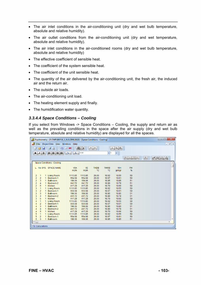
The air inlet conditions in the air-conditioning unit (dry and wet bulb temperature, absolute and relative humidity).

The air outlet conditions from the air-conditioning unit (dry and wet temperature, absolute and relative humidity).

The air inlet conditions in the air-conditioned rooms (dry and wet bulb temperature, absolute and relative humidity)

The effective coefficient of sensible heat.

The coefficient of the system sensible heat.

The coefficient of the unit sensible heat.

The quantity of the air delivered by the air-conditioning unit, the fresh air, the induced air and the return air.

The outside air loads.

The air-conditioning unit load.

The heating element supply and finally.

The humidification water quantity.

3.3.4.4 Space Conditions – Cooling

If you select from Windows -> Space Conditions – Cooling, the supply and return air as well as the prevailing conditions in the space after the air supply (dry and wet bulb temperature, absolute and relative humidity) are displayed for all the spaces.

FINE – HVAC - 103-

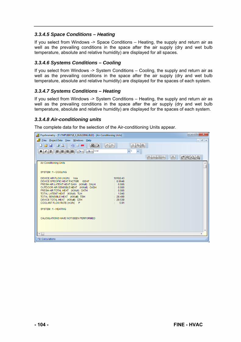
3.3.4.5 Space Conditions – Heating

If you select from Windows -> Space Conditions – Heating, the supply and return air as well as the prevailing conditions in the space after the air supply (dry and wet bulb temperature, absolute and relative humidity) are displayed for all spaces.

3.3.4.6 Systems Conditions – Cooling

If you select from Windows -> System Conditions – Cooling, the supply and return air as well as the prevailing conditions in the space after the air supply (dry and wet bulb temperature, absolute and relative humidity) are displayed for the spaces of each system.

3.3.4.7 Systems Conditions – Heating

If you select from Windows -> System Conditions – Heating, the supply and return air as well as the prevailing conditions in the space after the air supply (dry and wet bulb temperature, absolute and relative humidity) are displayed for the spaces of each system.

3.3.4.8 Air-conditioning units

The complete data for the selection of the Air-conditioning Units appear.

- 104 - FINE - HVAC

3.4 Examples

In this chapter three step-by-step examples are presented, which will help you understand in practice the basics of drawing in FINE HVAC. These simple examples aim mainly at helping you start drawing building entities (walls, openings etc.) along with heating and cooling networks. More specifically:

- Example 1, describes the steps of drawing a simple level and defining the spaces so as to calculate thermal and cooling loads.

- Example 2, describes the steps of drawing a simple two-pipes heating network, proceeding to the calculations and generating the necessary drawings. The same steps can be applied also to the single-pipe and fan-coils application.

- Finally, example 3, describes the steps of drawing an air-duct cooling network, proceeding to the calculations and generating the necessary drawings.

Apart from the following examples, you can watch the same steps (and much more) in the videos you will find in http://www.4msa.com/FineHvacENG.html.

3.4.1. Building design example In this example, the drawing of the adjacent simple building is described, including the steps from the beginning (creating a new project) to the end (calculating thermal and cooling loads) so that you can easily understand the function of FINE HVAC in practice.

For this example, we will import two architectural plan views that have been designed in AutoCAD although you can start drawing from scratch. If you have already designed the building in IDEA Architecture 11, you can skip this example.

1. From FILES menu, we select “New project”, type “Example_1” and press “Accept”.

2. From AutoBLD menu, we select “Building definition”, define as level 1 the “Basement” in elevation “-3” and from “File” we load its architectural drawing. Before we define the second level, we press “New” (so as to save the changes) and we follow the same steps for the second level, as it is shown below.

FINE – HVAC - 105-

When we finish, we press once again “New” and then “Accept” and automatically we defined the two levels with their architectural drawings.

3. Before we start drawing, we “Lock” the architectural drawings from the layers list on the left by pressing the “Lock” symbol as it is shown below. The name of the architectural drawing will be BASE_FLOO1_XREF for the first level, BASE_FLOO2_XREF for the second level etc.

- 106 - FINE - HVAC

4. From AutoBLD, we select Walls > Outer wall and in the properties window we define the height (3 m in our example) and the width (0.25 m) of the wall, the height and the width of the column (it will be automatically designed along with the wall), its type etc.

When we finish, we press “Accept” and we design the wall by defining three points:

- First, we click on the beginning of the wall (where the left red spot is, in the following image)

- Then, we click on the end of the wall (where the upper right red spot is) and

- Finally, we click on the side that the wall “grows” (where the down right red spot is).

You can enable the “Entity snaps” toolbar (or the “ESNAP” setting) so as to select easily the edges of the wall.

Continuing in the same way, we draw all the walls (inner and outer) of the ground floor.

FINE – HVAC - 107-

5. From AutoBLD, we select Opening > Door and in the properties window, we select the height (2.20 m in our example), the length (1 m), the type of the door etc.

When we finish, we press “Accept” and we design the door:

- First, we select the wall upon which we want to place the door.

- We click on the starting point of the door (where the left red spot is, in the following image)

- We click on the ending point of the door (where the upper right red spot is). As long as you have specified the length of the door, it is not necessary to specify this point exactly. You only need to specify a point near the start towards the side that the second point is located.

- Finally, we click on a point that shows the direction towards which the door will open (where the down right red spot is).

6. From AutoBLD, we select Opening > Window and in the properties window, we select the height (1.20 m in our example), the length (1 m), the rise (0.80 m), the type of the window etc.

When we finish, we press “Accept” and we design the window:

- First, we select the wall upon which we want to place the door.

- We click on the starting point of the window (where the upper red spot is, in the following image)

- We click on the ending point of the window (where the down red spot is). As with the door, as long as you have specified the length of the window, it is not necessary to specify this point exactly. You only need to specify a point near the start towards the side that the second point is located.

- 108 - FINE - HVAC

7. After drawing the walls, openings, doors etc. the ground floor has been designed as it is seem below. In the drawing, you can add the columns (from AutoBLD > Column) and the floors/ceilings (from AutoBLD > Floor - Ceiling).

In the following image, we have deactivated the architectural drawing, so as to have a better inspection of the drawing. To do this, go to AutoBLD > Layers management > and uncheck the “XREF” box.

8. We set the “North direction” symbol in the drawing, from AutoBLD > North direction.

9. In order to calculate the “Thermal Losses” and the “Cooling Loads”, we have to define the spaces of the ground floor.

From AutoBLD > Definition of plan view elements > Space definition, we choose “By point” and we zoom in, in a space:

- We click on an internal point of this space (where the left red spot is, in the following image)

FINE – HVAC - 109-

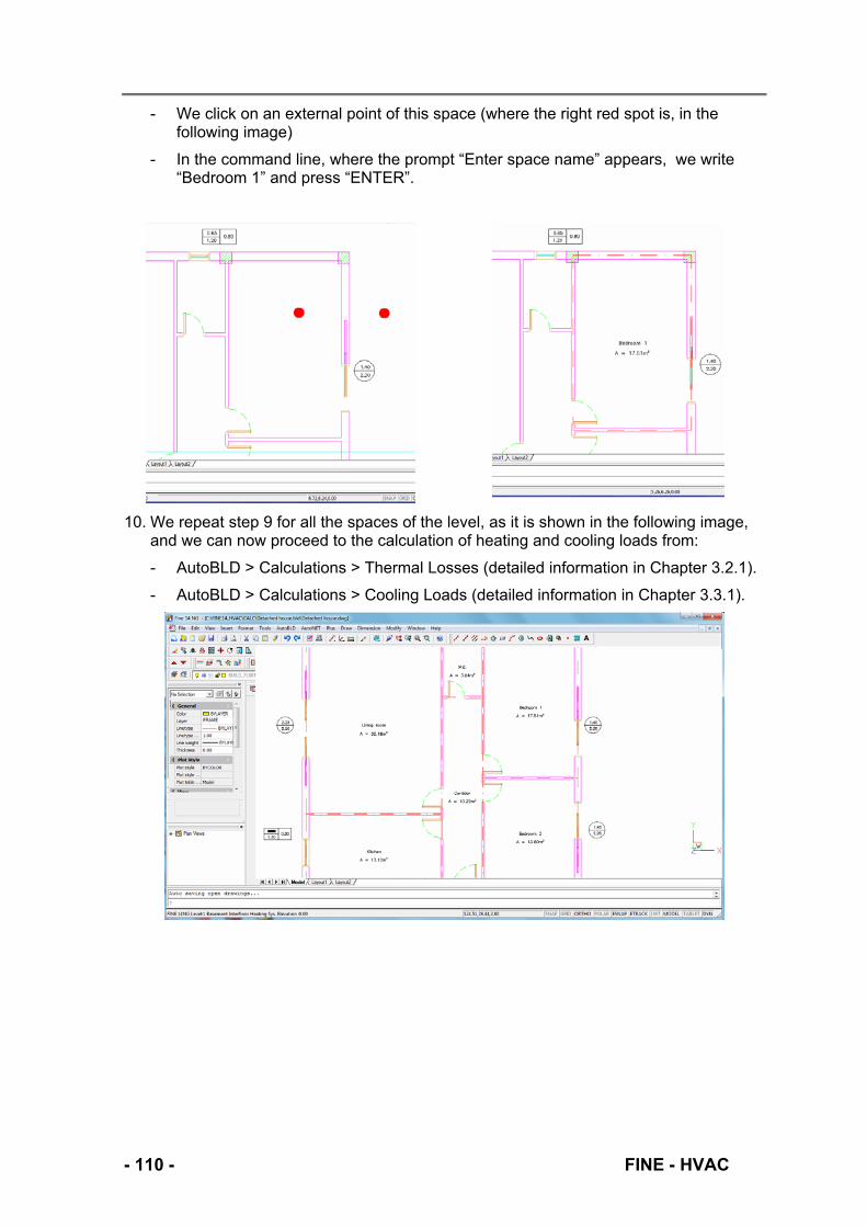
- We click on an external point of this space (where the right red spot is, in the following image)

- In the command line, where the prompt “Enter space name” appears, we write “Bedroom 1” and press “ENTER”.

10. We repeat step 9 for all the spaces of the level, as it is shown in the following image, and we can now proceed to the calculation of heating and cooling loads from:

- AutoBLD > Calculations > Thermal Losses (detailed information in Chapter 3.2.1).

- AutoBLD > Calculations > Cooling Loads (detailed information in Chapter 3.3.1).

- 110 - FINE - HVAC

3.4.2. Heating Network design example 1. Continuing working with the previous drawing, from AutoNET > Select application, we

choose “Two pipes system”.

Automatically, the “Two pipes system” toolbar is shown on the screen (see adjacent image) and you can either work from there or from the AutoNET commands.

2. First of all, we place the radiators in the rooms of the ground floor. From AutoNET > Radiators, we select the “IV505” radiator type, press “Accept” and place it in “Bedroom 1”. In this way, you can select on your own the type and the number of the radiators in each room.

Alternatively, from AutoNET > “Automatic radiators placement”, if we click on the “Living room” and press enter, the program automatically selects the number, the type of the radiators (depending on the “Thermal loads” of the space) and places them in the room. We repeat the same for the rest of the rooms.

3. From AutoNET > Supply pipe > we select “Straight supply pipe” and start drawing it between the walls and the radiators as it is seen in the following picture.

FINE – HVAC - 111-

4. The next step is connecting the supply pipe with the radiators and we do this easily by selecting from AutoNET > Supply pipe > Connect radiators to an existing pipe (or from the corresponding symbol of the toolbar):

- We click on the first radiator

- We click on the supply pipe next to it and finally

- Press ENTER and they are automatically connected.

- We repeat the step for all the radiators.

5. In order to place the vertical pipe that leads to the basement, we select from AutoNET > Main vertical pipes > Main vertical supply pipe:

- We click on the location we want to place the vertical pipe (in the command line you can see the “Enter XY location” prompt message).

- We type the height “-3” which is the starting point of the vertical pipe in this example (the basement elevation).

- We type the height “0” which is the ending point of the vertical pipe in this example (the ground floor elevation) and the supply vertical pipe is created.

- 112 - FINE - HVAC

6. From AutoNET > Supply pipe > we select “Straight supply pipe” and draw a part of the pipe connecting the horizontal to the vertical pipe as it is shown below.

You can use the “Entity snaps” toolbar (it is highlighted in the picture) to connect precisely the two pipes.

7. We repeat the steps 13-17 for drawing the return network (drawing vertical and horizontal pipes and connecting them with the radiators) and we have set the two pipes heating network for level 2.

8. By selecting the level of the basement (you can use to change levels or double click on the level’s name in the left side of the screen) we draw the horizontal supply and return pipe starting from each vertical pipe as it is shown below.

You can easily connect the horizontal to the vertical pipe using the “Perpendicular snap” point (highlighted in the following picture).

FINE – HVAC - 113-

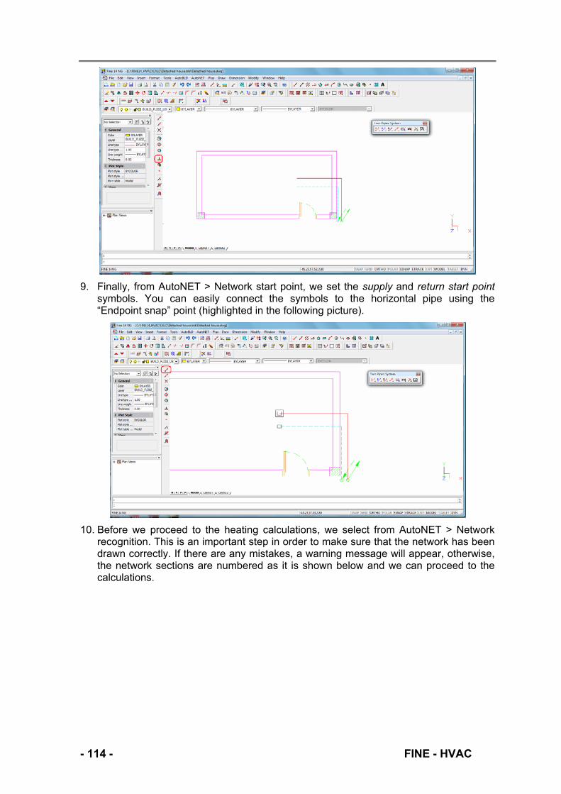
9. Finally, from AutoNET > Network start point, we set the supply and return start point symbols. You can easily connect the symbols to the horizontal pipe using the “Endpoint snap” point (highlighted in the following picture).

10. Before we proceed to the heating calculations, we select from AutoNET > Network recognition. This is an important step in order to make sure that the network has been drawn correctly. If there are any mistakes, a warning message will appear, otherwise, the network sections are numbered as it is shown below and we can proceed to the calculations.

- 114 - FINE - HVAC

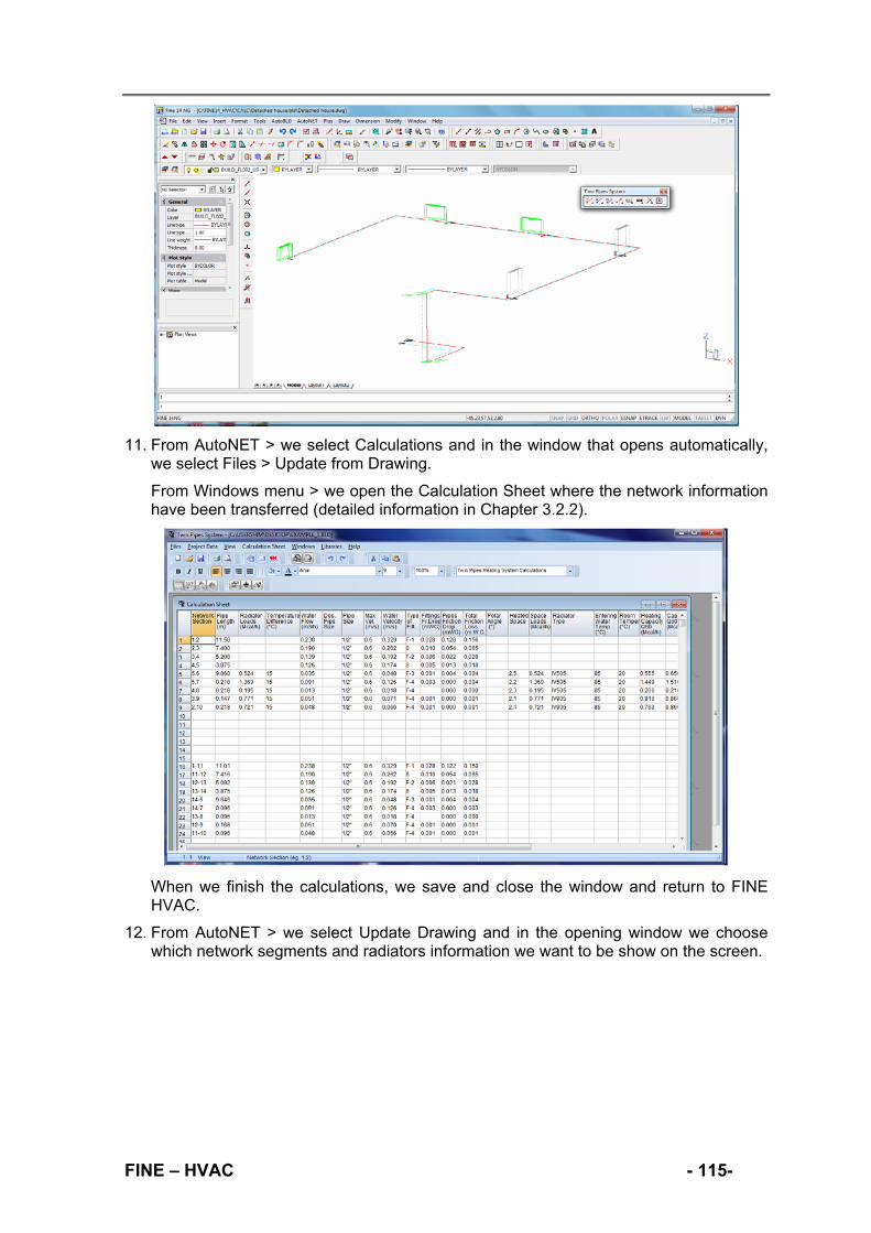
11. From AutoNET > we select Calculations and in the window that opens automatically, we select Files > Update from Drawing.

From Windows menu > we open the Calculation Sheet where the network information have been transferred (detailed information in Chapter 3.2.2).

When we finish the calculations, we save and close the window and return to FINE HVAC.

12. From AutoNET > we select Update Drawing and in the opening window we choose which network segments and radiators information we want to be show on the screen.

FINE – HVAC - 115-

By clicking “Auto Placement”, the selected information is shown in each level.

13. Finally, from AutoNET > we can select Convert single line to 3D and the program automatically creates 3D pipes in relation to the calculation results.

- 116 - FINE - HVAC

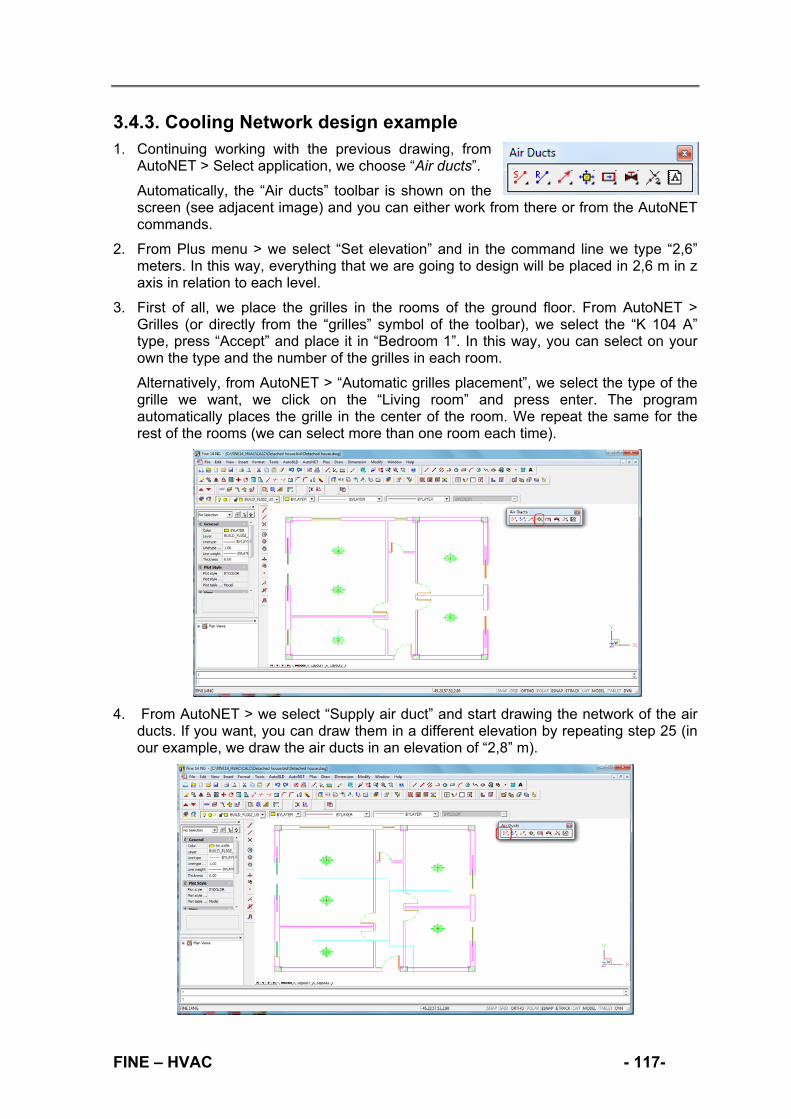
3.4.3. Cooling Network design example 1. Continuing working with the previous drawing, from

AutoNET > Select application, we choose “Air ducts”.

Automatically, the “Air ducts” toolbar is shown on the screen (see adjacent image) and you can either work from there or from the AutoNET commands.

2. From Plus menu > we select “Set elevation” and in the command line we type “2,6” meters. In this way, everything that we are going to design will be placed in 2,6 m in z axis in relation to each level.

3. First of all, we place the grilles in the rooms of the ground floor. From AutoNET > Grilles (or directly from the “grilles” symbol of the toolbar), we select the “K 104 A” type, press “Accept” and place it in “Bedroom 1”. In this way, you can select on your own the type and the number of the grilles in each room.

Alternatively, from AutoNET > “Automatic grilles placement”, we select the type of the grille we want, we click on the “Living room” and press enter. The program automatically places the grille in the center of the room. We repeat the same for the rest of the rooms (we can select more than one room each time).

4. From AutoNET > we select “Supply air duct” and start drawing the network of the air ducts. If you want, you can draw them in a different elevation by repeating step 25 (in our example, we draw the air ducts in an elevation of “2,8” m).

FINE – HVAC - 117-

5. The next step is connecting the supply air duct with the grilles and we do this easily by selecting from AutoNET > Connect grilles to existing duct (or from the corresponding

symbol of the toolbar). Instead of this command, you can use the “Connect grilles to existing duct with flexible duct”:

- We click on the first grille

- We click on the supply air duct next to it

- We press ENTER and they are automatically connected.

- We repeat the step for all the grilles (we can connect more than one grille to an air duct each time).

6. In order to place the vertical air duct that leads to the basement, we select from AutoNET > Vertical air duct > Supply duct:

- We click on the location we want to place the vertical duct (in the command line you can see the “Enter XY location” prompt message).

- We type the height “-3” which is the starting point of the vertical duct in this example (the basement elevation).

- We type the height “2,8” which is the ending point of the vertical pipe in this example (from the “Set elevation” command we have set the elevation we are drawing the air ducts in the ground floor in “2,8” m) and the vertical duct is created.

- 118 - FINE - HVAC

7. From AutoNET > we select Supply air duct and draw a duct connecting the horizontal to the vertical air duct as it is shown below.

You can use the “Entity snaps” toolbar (it is highlighted in the picture) to connect precisely the two ducts.

8. By selecting the level of the basement (you can use to change levels or double click on the level’s name in the left side of the screen) we draw a horizontal supply air duct starting from the vertical duct as it is shown below.

(ou can easily connect the horizontal to the vertical duct using the “Perpendicular snap” point).

Finally, from AutoNET > Network start point, we set the supply start point symbol. You can easily connect the symbol to the horizontal pipe using the “Endpoint snap” point (highlighted in the following picture).

9. If you want, you can easily draw the return air ducts network by repeating the steps 26-31.

FINE – HVAC - 119-

10. Before we proceed to the cooling calculations, we select from AutoNET > Network recognition. This is an important step in order to make sure that the network has been drawn correctly. If there are any mistakes, a warning message will appear, otherwise, the network sections are numbered as it is shown below and we can proceed to the calculations.

11. From AutoNET > we select Calculations and in the window that opens automatically, we select Files > Update from Drawing.

From Windows menu > we open the Calculation Sheet where the network information have been transferred (detailed information in Chapter 3.3.3).

When we finish the calculations, we save and close the window and return to FINE HVAC.

12. From AutoNET > we select Update Drawing and in the opening window we choose which air ducts and grilles information we want to be show on the screen.

- 120 - FINE - HVAC

By clicking “Auto Placement”, the selected information is shown on each level.

13. From AutoNET > we select Convert single line to 2D, in the command line we type “S” (as we only have supply network) and the program automatically creates 2D pipes in relation to the calculation results.

FINE – HVAC - 121-

14. Finally from AutoNET > we select Convert single line to 3D and the program automatically converts the network into 3D in relation to the calculation results.

- 122 - FINE - HVAC