1

FINELab™ QC System

Tutorial

FINELab Start Screen

2

CONTENTS

1. QC Testing .................................................................................3

2. Golden Average Driver / Preproduction......................................5

3. Edit Limits...................................................................................6

4. Measurement .............................................................................8

5. Test in a Normal room..............................................................11

6. Subwoofer in NearField ............................................................14

7. FINEBuzz – Rub & Buzz Detection ..........................................16

8. Thiele / Small (TS) Parameters ................................................18

9. Typical Test Setup Procedure ..................................................19

3

The FINELab Start Screen is shown on page 1. Without logging in all users can directly load

Measurement Files and view Statistics from automatically saved QC test series. An example is shown in the next picture which is the result of a previous test series:

Figure 1 - Statistical Result of previous QC Test Series

The frequency responses of all units tested are shown in the upper window as green lines, with the tolerance limits shown in red. The average of all responses is shown in violet, however you can select

to view all Pass or Fail for SPL, Impedance, Sensitivity or Polarity as you wish plus getting the test yield for each.

The middle window shows the same responses as above, but now plotted relative to the reference (blue). For example a change in sensitivity is very easy to see this way.

The Impedance with limits is plotted in the lower window. The average of all responses is shown as the violet curve and the reference as the blue response.

QC Testing This time I log in as an engineer with my own password and select “2,5in_Fullrange2” and “Run that

Test”. The following screen appears:

4

Figure 2 - FINELab Test Details

After filling in the Batch number and customer name this series will start with #1 and automatically

count up as you test. If you enter the last tested number instead, FINELab will count up from that.

Figure 3 - FINELab Test Display: SPL FAIL at 3.5 kHz

As a good rule I will start by testing my reference driver by pressing “Single/Re-Test”, which ensures that this initial reference test will not be saved in the test series. (I can accept small sensitivity changes of the measured reference driver response if caused by a change in environment

temperature).

I start the test by pressing

5

The first driver is now tested with a fast sine sweep. In this case the speed was chosen to be 2.5

seconds, so the tester can listen for distortion and Rub & Buzz while testing. The measured response is shown in the upper window as a green curve, with the response limits in red.

If the measured response is exceeding the limits, the colour changes to yellow and SPL: FAIL is

reported in the right centre window. The large centre window is showing the measured response compared to the reference driver. Here it is much easier to see when the response is outside the

limits, see the example in Fig. 3.

The sensitivity can be defined as an average over a frequency range, in this case 95.1dB (700-1200Hz). The impedance is measured with the same sweep. That saves time and ensures that the

level and resonance Fs is the same as in the frequency response. (A too low current may show Fs

much higher). The polarity is also checked and reported OK. The next line is (Limits-) Compensation: This is a kind of Sensitivity Controlled Floating Limits. When

the response is measured it is allowed to move within the limits as determined by the sensitivity

tolerance. Finally the actual yield of the test is calculated. As soon as End Test is pressed the Statistics of the series is displayed and the user can view rejects

etc (see page 3).

Golden Average Driver / Preproduction

Figure 4 -Golden Average Driver Auto Finder

6

When starting a new production, the most important is to find the unit which is closest to the

average of the good units, so it can be used as reference. Our pilot run consists of 17 woofers for a 2-way system, which are sorted using the Preproduction

feature, see Fig. 4. The highlighted driver response (yellow) is Serial No.8 in the table and is the best

match to the average i.e. the Golden Average Unit.

Note that driver No. 7 is deselected in the table because that response was considered non-typical

and should not disturb the average.

Should it be necessary to find a similar reference driver later, that can be found by selecting “Best

Match to Reference”.

Edit Limits From the statistics in Fig. 1, I can see that the rejected responses have a dip at 3.5 kHz, but actually

it is the slope of the peak which has changed. Therefore it makes sense to adjust the limits to allow

that. Select “Edit that test” from the menu (Fig. 5):

Figure 5 - Menu

7

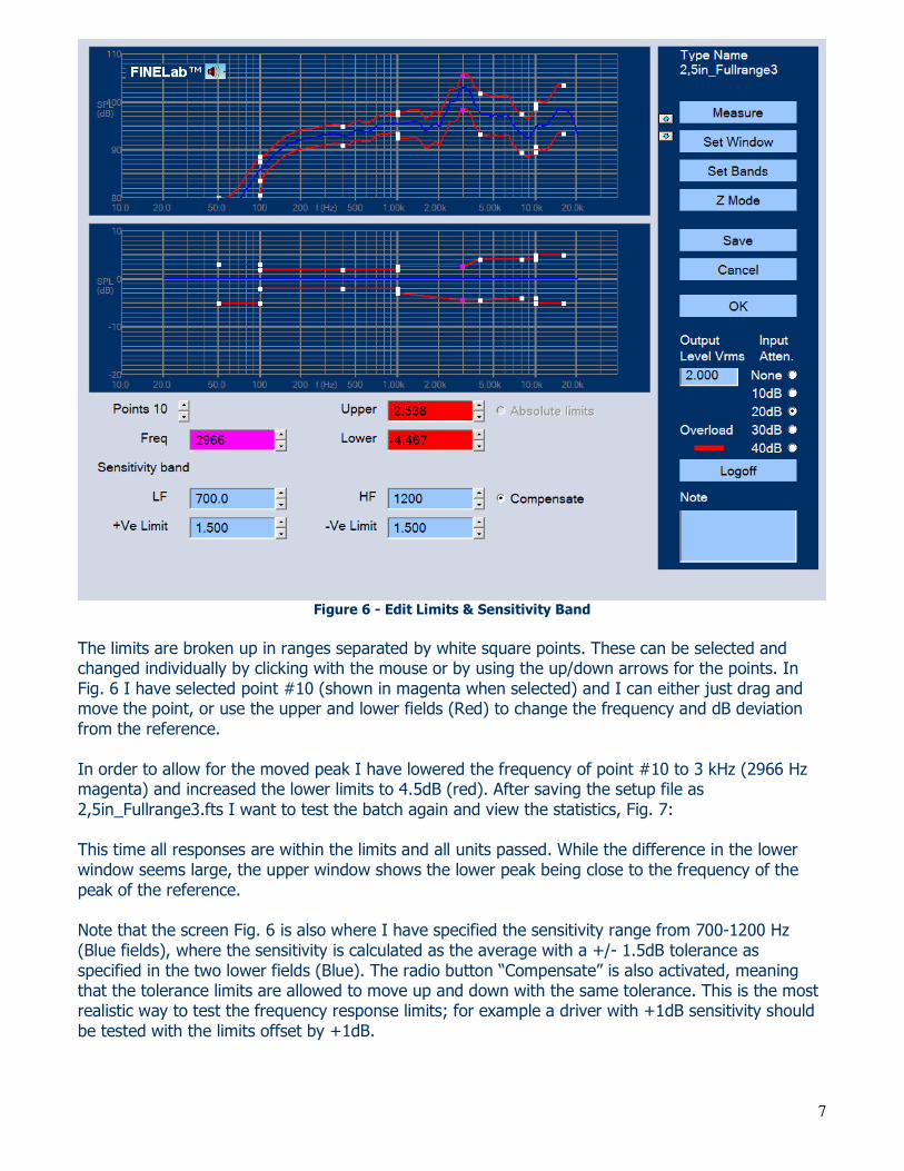
Figure 6 - Edit Limits & Sensitivity Band

The limits are broken up in ranges separated by white square points. These can be selected and changed individually by clicking with the mouse or by using the up/down arrows for the points. In

Fig. 6 I have selected point #10 (shown in magenta when selected) and I can either just drag and move the point, or use the upper and lower fields (Red) to change the frequency and dB deviation

from the reference.

In order to allow for the moved peak I have lowered the frequency of point #10 to 3 kHz (2966 Hz magenta) and increased the lower limits to 4.5dB (red). After saving the setup file as

2,5in_Fullrange3.fts I want to test the batch again and view the statistics, Fig. 7: This time all responses are within the limits and all units passed. While the difference in the lower

window seems large, the upper window shows the lower peak being close to the frequency of the

peak of the reference. Note that the screen Fig. 6 is also where I have specified the sensitivity range from 700-1200 Hz

(Blue fields), where the sensitivity is calculated as the average with a +/- 1.5dB tolerance as

specified in the two lower fields (Blue). The radio button “Compensate” is also activated, meaning that the tolerance limits are allowed to move up and down with the same tolerance. This is the most realistic way to test the frequency response limits; for example a driver with +1dB sensitivity should

be tested with the limits offset by +1dB.

8

The output drive level from the built-in amplifier is here set to 2Vrms, which is producing a

reasonably high SPL without overloading this 2.5 inch full range speaker. Fig. 6 shows overload (Red) and the attenuator should be set one step lower.

Figure 7 – SPL Statistics with adjusted limits

Measurement In this chapter I will show how an entire test setup is created. I select “New” from the menu and get

the following window (Fig. 8), where I first specify the File name:

Figure 8 – Full-range SPL Template

9

I have selected the “Full-range” standard (Template) from the drop-down menu, which contains

generic standard templates for the most used speakers. The 2.5second sweep time is slow enough for the tester to listen for bad sounding drivers during normal testing. However the best is to find the Rub & Buzz using the new FINEBuzz feature, which can be set in “Edit QC Test”.

The limits can be specified in up to 8 bands; in this case the standard template is using 7 bands with +/-2dB from 100-1000 Hz, which is the stable mid-band region before break-up. The standard limits

“Window” or “Mask” is opening up towards low and high frequencies, where we expect more

deviation due to shifts in resonance frequency Fs and break-up at high frequencies. The user can

change the limits any time if needed.

Figure 9 – Full-range Impedance Template

After accepting the SPL limits the Impedance Template appears Fig. 9, with just one range specified from 50 to 10,000 Hz. The deviation is here defined as a ratio because we are measuring impedance.

The max and min ratios are 1.2 (20%) and 0.8 (80%) which I choose to use for now. I may later need to open the limits to allow for variation of Fs.

Now I measure the speaker by clicking the “Measure” button. After the sine sweep is played the next button down is “Set Window”, which brings up the Time Domain window Fig. 10:

The impulse response is shown in the upper half and the windowed frequency response below. Most of the buttons in the upper half are automatically providing scaling of the impulse response. The time before the impulse is arriving is called the “Flying Time”, which is the travel time (in air) from the

speaker cone and until it reaches the microphone. The “Auto delay” button will find this time

automatically and is on by default.

Note: If you move the microphone closer to the speaker after saving the Setup file (*.fts), you may miss the initial impulse and the frequency response will look “strange”. If you know that the microphone could move say 1cm closer, you should reduce the Initial Delay setting by 2 (1 gives appr.0.7cm).

10

Therefore I only need to care about the end of the impulse, which is indicated in the lower right

field: I have chosen 1000 samples or 20.8mS corresponding to 50Hz (using the 1/f ratio) using a cosine/Hann window (Cos window Out). 20.8mS is a long time, but is useable in this case because a large well damped test box was used with the microphone at ~20cm distance, which can be

calculated from the initial delay of 562.5uS, giving the actual distance of 19.3cm.

The final windowed frequency response is useable from about 50Hz, showing good response from

150 Hz and almost up to 20 kHz. The acoustic phase response is shown as the dashed line and is

well behaved and close to minimum phase.

Figure 10 - Time Window settings

After OK the Z Mode button is pressed to enter the impedance limits screen Fig. 11. First I pressed

“Measure” to make sure the measured curve is the actual impedance. I have chosen to modify the pre-defined limits of +/-20% around the Fs impedance peak to allow for

a natural variation in production. That was done the easy way by simply clicking the white squares

and dragging the limits with the mouse. Note that the limits are automatically updated in both windows when dragging.

Since the impedance measurement is purely electrical, the range and time window is already defined

when the “Auto delay” is active. So there is no need to open the “Set Window”. When the limits are OK click Save.

11

Figure 11 – Impedance Limits, adjusted

In this window the engineer can also add a note, which will be displayed for the tester. A typical note

is shown in Fig.11:

[NB! This driver must be tested in cabinet)

Test in a Normal room Fig. 12 shows the response of a satellite speaker tested at 1m in a normal room with the microphone in line with the tweeter, which is the normal listening axis. The tweeter of the speaker was about 82cm above the floor. Note that the low end response is limited around 300Hz. This is unfortunately

not the true response, but the result of a poor measurement.

12

Figure 12 - Satellite Speaker tested in Normal Room at 1m

The Time domain impulse response of the satellite is shown in Fig. 14. The main impulse is arriving after approximately 3mS corresponding to 1m (the speed of sound is ~343m/s or 0.343m/mS).

However you can see another strong impulse arriving already about 2.5ms after the main impulse.

That is the reflection from the floor, which is only 82cm below the speaker and microphone, Fig. 13.

Figure 13 - Satellite close to floor, Red is Reflection

13

Figure 14 - Time Response of Satellite at 1m microphone distance and 82cm above floor

The short time between the two impulses is the reason for the poor low frequency response (Fig. 14)

Using the 1/f ratio the 2.5ms will only allow 400 Hz as the lowest frequency. Since we are using a cosine window we may extend that to 2.7-3mS, but that does not really help.

Fig. 13 is illustrating the problem where the reflection from the floor is too close to the main signal, because there is little difference between the direct distance (green arrow) and the reflection path (red arrows). We can do two things to improve that: Move the microphone closer to the speaker

and/or move both speaker and microphone further away from the floor (or other surfaces).

14

Figure 15 - Satellite and microphone moved up to 154cm above floor, microphone distance 0.5m

I have done both in Fig. 15, by moving both the microphone and speaker up to 154cm from the floor

and because the speaker is quite small it is safe to adjust the microphone distance to 0.5m (the distance to the other walls and ceiling is equal to or larger than 154cm). This time we get the

reflections much later and can use a window of 10.4ms. Therefore we get the real low frequency

response of the satellite, starting from approximately 150 Hz.

Subwoofer in NearField The final example is an 8 inch subwoofer which I choose to measure without any baffle or cabinet, using the NearField Measurement method with the microphone very close to the cone. This method

is quite powerful and will show the full low end response as if the driver was placed in a very large baffle (~infinite baffle). The only drawback is that the response is only valid at low frequencies

(below break-up). The -1dB limit is around 500 Hz for an 8 inch woofer so the LF response and sensitivity can be measured well, and the subwoofer roll off can be estimated.

The time domain response is shown as Fig. 16, and no reflections are observed. In fact I have used the default 200ms to enable measurement down below 20Hz. The final test screen for the 8 inch

subwoofer is shown in Fig. 17. The limits are tight from 100-500 Hz which is the piston range before

break-up. The sensitivity is measured as an average from 100-400Hz.

FINELab QC 2 has a Subwoofer2.5s-5k.fts setup file, which is limited to 5k and has FINEBuzz

enabled. This setup is recommended for subwoofer near-field testing.

15

Figure 16 - 8 inch Woofer measured in NearField

Figure 17 - 8 inch Subwoofer Test in NearField

16

FINEBuzz – Rub & Buzz Detection On the production line it is necessary to check all units for bad sound. The frequency response and impedance of a driver or system may well be within limits but can unfortunately still sound bad, for

example due to a rubbing voice coil or a rattle from the cabinet.

The new FINEBuzz detection method is based on the latest Danish research on hearing mechanisms, and uses a completely new algorithm to find the annoying sounds, which cannot be detected with conventional methods like THD, high harmonics or IM distortion. The new method is extremely

sensitive and can detect even the smallest buzzing tinsel in a tweeter.

After selecting a woofer setup to 5 kHz and measuring the response of a good woofer with acceptable rub and buzz, I press the button “Setup R&B Test” to bring up the following screen,

Fig.18:

Figure 18 - FINEBuzz Setup Screen

The rub and buzz is normally concentrated at low frequencies where the driver excursion is high. These annoying sounds, contains high harmonics where the ear is most sensitive, especially around

1- 3 kHz. FINEBuzz has a sweeping filter to pick up the rub and buzz, which should be set to a ratio between 5 -10 (5-10x test frequency). In this example I will test a 6.5inch woofer and use the default ratio of 8 (8-12 is recommended for woofers and 5-8 is good for tweeters).

In this case I have set the white limit line only 5 dB over the acceptable rub and buzz +noise level (blue columns) where the default is 10 dB. (See also the note below).

The display range was set to 5000 Hz, but the “Recalculate” button will adjust all to fit the test

resolution etc. After OK and Save, it is time to start testing.

Note: Setting the FINEBuzz limit less than 10 dB requires very silent test conditions! Use a separate test chamber and avoid noise sources like air guns, fans and bumping carts and pallets.

17

Fig. 19 shows a woofer which failed due to a rubbing voice coil, indicated by the red columns where the rub and buzz is above the white maximum line.

Figure 19 – 6.5inch Woofer with rubbing Voice Coil found with FINEBuzz

It is possible to test Rub & Buzz in 1 second, but I recommend using the longer 2.5s setup, because a fast sweep may not contain enough energy to find very small resonances. In the above example, I

used the 20-5kHz sweep, which further concentrates the energy in this band. Likewise the tweeter2.5s_200-20k setup is ideal for finding small resonances like buzzing tinsels in

tweeters. Fig. 20 shows a tweeter with very subtle buzzing tinsel at 900Hz.

Figur 20 - Tweeter with very subtle buzzing tinsel at 900Hz

18

Thiele / Small (TS) Parameters Finally I want to measure the TS parameters of a 10 inch subwoofer. Pressing “Edit TS Test” from a previously defined QC Test will show the screen in Fig 21:

Figure 21 - TS Parameters of 10inch Subwoofer

First I need to input the cone area Sd and Re. I choose to input the effective diameter of 20.7cm

(centre of surround) and Sd will automatically be calculated. FINELab QC can estimate Re from the impedance curve, but in order to get the best accuracy I have measured Re=3.04 ohms with a precise Multimeter (DVM). That value is fixed by lock [v]. Now I press “Measure” to get the

impedance curve (green).

I could choose the standard Added Mass or Added Box method, but the Fixed Mass option is much more accurate. However I must cut a typical woofer, so I can weigh the cone + Voice Coil + half

surround + half spider (including dust cap and glue etc.). This mass (Md) is entered as Diaphragm

Mass which causes the air load mass (Mair) to be calculated, Md + Mair=Mms.

When the “Calculate” button is pressed, FINELab will calculate all the TS parameters by fitting a

simulated impedance curve (red) in the chosen frequency range. In this case we get a very good fit

around Fs, which is important for getting accurate TS parameters.

Qts is calculated as 0.37 with Fs= 30.2Hz, but we also get the sensitivity SPL= 88.76 dB/2.83V.

We must accept a large variation in Qts, because it depends strongly on Fs. Therefore FINELab QC also calculates the ratios Fs/Qts=82.41 and BL2/Re=40.32. These ratios are more important for controlling the bass response than Qts and Fs and other parameters.

19

Typical Test Setup Procedure In this chapter I will summarise the necessary steps in a typical test setup:

1. Log in as Engineer 2. Select a test specification as close as possible to the kind of speaker you want to test. 3. Select “New Based On” and input a name for the test

4. Specify a suitable amplifier Output Level (Vrms). Choose a level so the driver will move close

to half of Xmax for woofers and around 1W or less for tweeters. 5. Press “Measure” to do the first sweep test with Input Attenuation set to: None

6. If you see the red “Overload” light, then select one step lower Input Attenuation and

“Measure” again. Repeat until there is no overload

7. Press “Set Test Window” to enter the Time Domain Window a. Check that the large pulse is close to 0mS. That is normally done by the “Auto Delay”.

If not adjust the “Initial Delay”. (Auto Delay is by default 5%. This can be changed in

Admin. A higher number will prevent FINELab from trigging on noise) b. The dashed curve is the acoustic phase response which will show less variation when

the large pulse is close to 0mS c. Input a suitable number of samples in: (Cos Window Out / End (samples))

i. If you are using an anechoic room or really well damped box use ~10-20mS ii. If you are using a normal room or standard test box use ~3-10mS

iii. If you are measuring in the near field you may use the full 200mS. d. The idea is to choose a window which will pass the decaying pulse, but avoid the

reflections which are arriving later (see for example Fig. 13)

e. The window may extend to include some reflections in the end, because the cosine

window will attenuate much towards the end 8. Select “Set Bands”

9. Choose a suitable SPL tolerance limit standard

a. Modify the tolerances and bands if you know how much you need

b. If you do not know how much to change the limits, then use the standard one and check the response statistics before considering changes to the limits

10. Press “Z mode” to enter the Impedance window

11. Press “Measure” to do a first impedance sweep test 12. Use the up/down arrow buttons to scale the impedance curve as necessary 13. You do not need to press “Set Window” to enter the Time Domain Window, but you can.

14. Select “Set Bands” if you want to choose standard limits, OR 15. Click and drag the white squares to suitable production limits.

16. Press “Save” when you are satisfied with the limits 17. You should now run the test file you have created with a small number of units (Test Batch)

to verify your settings and limits. Press “End Test” when done and the statistics Display will automatically appear showing all the responses with your limits. You can choose to display

good/rejected SPL, Impedance, Sensitivity or Polarity. 18. Select “Review Old Data” and view the Pre-Production of your Test Batch “Pre-Prod” 19. The Pre-Prod window highlights the Golden Reference (You can de-select non-typical curves).

20. Press “Edit that test” if you want to change the limits according to the statistical results

Peter Larsen

www.loudsoft.com

Agern Alle 3 – 2970 Horsholm – Denmark

Tel: (+45) 4582 6291 - Fax (+45) 4582 7242