Fines reduction and energy optimisation in aggregates production Matthew James Amor Ruszala Supervisors: Dr Neil Rowson Mr Jon Aumônier Dr Phil Robbins MRes Chemical Engineering Sciences The University of Birmingham May 2013
Transcript
Fines reduction andenergy optimisation inaggregates production
Matthew James Amor Ruszala
Supervisors: Dr Neil Rowson
Mr Jon Aumônier Dr Phil Robbins
MRes Chemical Engineering Sciences
The University of Birmingham
May 2013
University of Birmingham Research Archive
e-theses repository This unpublished thesis/dissertation is copyright of the author and/or third parties. The intellectual property rights of the author or third parties in respect of this work are as defined by The Copyright Designs and Patents Act 1988 or as modified by any successor legislation. Any use made of information contained in this thesis/dissertation must be in accordance with that legislation and must be properly acknowledged. Further distribution or reproduction in any format is prohibited without the permission of the copyright holder.
M. J. A. Ruszala MRes Chemical Engineering Sciences May 2013
1
ABSTRACT
Aggregates production is a huge global industry which uses an enormous amount of energy and
produces a massive amount of unsaleable fines. By reducing the amount of energy used per tonne of
material produced and/or the amount of fines produced, it would make a quarry more efficient and,
therefore, more environmentally friendly and profitable. This research looks at modelling
Mountsorrel Quarry, a granite quarry in the UK, using JKSimMet and Split-Desktop software packages
in conjunction with the EU project, EE-Quarry. XRF analysis of Mountsorrel Quarry granite found that
it contains a number of oxides, predominantly SiO2 (63.3%) and Al2O3 (16.8%), and XRD analysis
found it contains the crystalline structures of quartz (SiO2) and albite, calcian, ordered
(Na,Ca)Al(Si,Al)3O8). Samples submitted to drop-weight tests confirmed Mountsorrel Quarry granite
as an extremely hard granite and rock fracture (t10) data and energy of comminution (Ecs) data were
obtained from analysing the results.
Split-Desktop image analysis software was utilised to determine the particle size distribution (PSD) of
the primary crusher feed, as it contains particles too large to screen manually. It was also found that
0.8% of the feed is fines, which at Mountsorrel Quarry are classed as particles smaller than 5 mm,
and that no particles were larger than 3810 mm. JKSimMet was used to create a flowsheet of
Mountsorrel Quarry, and the crusher product PSDs were simulated and was found to have strong
correlations with experimental data, especially in the fines region, with a mean difference of 1.0%.
The simulated primary crusher product PSD showed that it contains 5.9% fines, and a simulation over
the entire quarry showed the product to be within the size range produced at Mountsorrel Quarry,
and with a simulated fines content of 13.4%. When the closed side setting on the primary crusher
was altered from 165.1 mm (the operating size on site) to 100.0 mm, it increased the amount of fines
produced by 45%, increased the power draw by 140.6 kW, but reduced the overall plant production
of fines by 18%.
M. J. A. Ruszala MRes Chemical Engineering Sciences May 2013
2
Two blasts were undertaken on adjacent rock faces which had identical blast designs, other than the
order of deck detonation, with the first blast detonating the bottom deck before the top and vice
versa in the second blast. For each blast, measurements of the feed PSD to the primary crusher, the
number of particles that required secondary breakage on the quarry floor, acoustic levels and
vibration readings were measured and no significant difference was identified between the two
blasts in any of the parameters measured.
In conclusion, a working model of Mountsorrel Quarry has been made in JKSimMet that has been
validated against data from site and Split-Desktop has been used to simulate the primary crusher
feed PSD, something that was previously unknown. The effect of reversing the order of deck
detonation in a two deck blast was also analysed but with no significant difference between the two
blasts found.
M. J. A. Ruszala MRes Chemical Engineering Sciences May 2013
3
ACKNOWLEDGMENTS
I would like to express my greatest gratitude to all the people who have helped and supported me
throughout my project. I am truly thankful and indebted to my supervisor, Dr Neil Rowson from the
University of Birmingham for his advice and direction throughout, as well as my secondary supervisor,
Dr Phil Robbins. I would also like to thank Jon Aumônier, at MIRO, who provided the funding for this
research and provided plenty of helpful ideas. I would not have been able to have completed this
research wit out the help Ian Brown, Mick Collins, Simon Edwards, Steve Mee and everybody else at
Lafarge Aggregates’ Mountsorrel Quarry who very kindly explained the workings of the quarry and
were extremely cooperative in helping me to collect my data while putting up with me interrupting
their work. Moreover, I would like to thank Dr Rob Farnfield and Dr Mark Pegden from EPC, who
helped to coordinate the blasting experiments and gave me help and advice in the field of explosives
and blasting, and Christopher Bailey from JKSimMet and Brian Norton from Split-Desktop who helped
me with my queries with their software. Last and by no means least I would like to thank Dr Richard
Greenwood from the University of Birmingham for his help on and off site, Prof Sam Kingman of
Nottingham University for kindly allowing me to use his drop-weight tester, and Jon Rowson for
compiling some tables of data on JKSimMet.
M. J. A. Ruszala MRes Chemical Engineering Sciences May 2013
4
TABLE OF CONTENTSABSTRACT .......................................................................................................................................... 1
Appendix I – MSDS ........................................................................................................................93
Appendix II – PSD and power data for EE-Quarry ...........................................................................98
Appendix III – Blast vibration and acoustic readings ....................................................................153
M. J. A. Ruszala MRes Chemical Engineering Sciences May 2013
6
TABLE OF FIGURESFigure 1: Site map of Mountsorrel Quarry with the quarry, primary crusher, stock area and rail sidings (inset) shown (Lafarge Aggregates Ltd, 2012). ...................................................................................27
Figure 2: Diagram of a cone crusher where the rock material is fed into the top of the crusher and the eccentric rotation compresses the rock between the cone and the concaves until it is small enough to fit through the sizing gap (which is set at a specific width) and is discharged (British Geological Survey, n.d.). .................................................................................................................................................28
Figure 3: Diagram of a cone crusher where the rock is fed into the crushing chamber and the main shaft gyrates, thus compressing the rock against the liner wall until it is small enough to fit through the sizing gap (which is set at a specific width) and is discharged (Primel & Tourenq, 2000). .............29
Figure 4: Schematic to show the basic principles of XRF spectrography, where x-rays are fired at a test sample and the resultant backscattered x-rays are recorded by a detector (Thermo Scientific, n.d.). 30
Figure 5: Diagram of an XRF spectrometer with the presentation and control equipment excluded (Jenkins et al., 1995). ........................................................................................................................30
Figure 6: Schematic to show how XRF spectrography works. When the x-rays are fired at the sample, they collide with the atoms contained in the sample causing the ejection of electrons from various shells in the atoms and the emission of x-rays. The x-rays that are emitted are uniquely characteristic of the element from which they were emitted ad they can therefore be used to decipher what elements are present in a sample (Thermo Scientific, n.d.)................................................................31
Figure 7: Plot of elements present in Mountsorrel granite obtained by XRF analysis. ........................32
Figure 8: Schematic diagram of an XRD diffractometer (Thermo ARL, 1999). .....................................33
Figure 9: Overall compound spectrum (black peaks) with quartz (SiO2; red lines) and albite, calcian, ordered (Na,Ca)Al(Si,Al)3O8; blue lines) obtained by XRD analysis. .....................................................34
Figure 10: Diagram representing the three ways in which cracks can be propagated in a rock particle (Chang et al., 2002) ...........................................................................................................................35
Figure 11: Diagram showing the various ways that single particle breakage tests can be undertaken, including single impact, double impact and slow compression methods (Tavares, 2007). ..................36
Figure 12: Schematic diagram of a drop-weight test machine where the drop-weight (of known weight) is raised to a set, known height above the particle sample (h0) before being dropped onto the particle sample and compressing it between the drop-weight and the anvil which usually results in fracturing of the sample (Chau & Wu 2007). .....................................................................................37
Figure 13: Graph showing the varying power draw and energy used per tonne of material crushed when the CSS is varied from 10 mm to 55 mm for Mountsorrel Quarry granite in a cone crusher with a feed rate of 150 t h-1, ET of 25 mm and a fixed feed PSD calculated using JKSimMet. ......................39
M. J. A. Ruszala MRes Chemical Engineering Sciences May 2013
7
Figure 14: Image of a dumper truck leaving the primary crusher at Mountsorrel Quarry after unloading but still carrying some rock particles. ................................................................................46
Figure 15: Split-Desktop validation curves of three tests against manual sieving data from Liu & Tran (1996; top) and a later study (bottom). Please note that the x axis on the top graph is linear whilst it is logarithmic on the bottom graph (Split-Desktop, 2001)..................................................................47
Figure 16: Comparison of PSDs obtained from Split-Desktop (line) and sieving (dots) over 6 surveys (Kemeny et al. 1999). ........................................................................................................................47
Figure 17: Initial image of a dumper unloading into the primary crusher at Mountsorrel Quarry before being analysed with Split-Desktop to determine the PSD. .................................................................48
Figure 18: Various delineations (navy blue lines) of the initial picture where the amount of delineation is A<B<C<D. ....................................................................................................................49
Figure 19: The delineated image of the feed to the primary crusher at Mountsorrel Quarry (A) and the image editing (B), with delineation (dark blue lines), scaling (black line spanning the crusher dome), fines addition (red) and areas that are not rock removed (light blue). ...................................50
Figure 20: PSD cumulative curve (left) and PSD histogram (right) obtained using Split-Desktop and plotted with a logarithmic x axis. .......................................................................................................50
Figure 21: Image of the PSD feed for a crusher in JKSimMet. .............................................................51
Figure 22: PSD of the feed to the primary crusher at Mountsorrel Quarry obtained using Split-Desktop. The error bars represent standard error. ............................................................................53
Figure 23: Flowsheet of Mountsorrel Quarry created using JKSimMet with key. ................................58
Figure 24: Image of the input field of the rock fracture data (t10) in JKSimMet. ..................................60
Figure 25: Image of the input field of the energy of comminution data (Ecs) in JKSimMet ..................60
Figure 26: Graph to show the simulated Mountsorrel Quarry primary crusher product PSD obtained using JKSimMet. ................................................................................................................................61
Figure 27: Graph to show the simulated (red) and experimental (blue) output PSDs from cone crusher 1A at Mountsorrel Quarry. ................................................................................................................62
Figure 28: Graph to show the simulated (red) and experimental (blue) output PSDs from cone crusher 1B at Mountsorrel Quarry. ................................................................................................................63
Figure 29: Graph to show the simulated (red) and experimental (blue) output PSDs from cone crusher 2 at Mountsorrel Quarry. ..................................................................................................................63
Figure 30: Graph to show the simulated (red) and experimental (blue) output PSDs from cone crusher 3 at Mountsorrel Quarry. ..................................................................................................................64
M. J. A. Ruszala MRes Chemical Engineering Sciences May 2013
8
Figure 31: Graph to show the simulated (red) and experimental (blue) output PSDs from cone crusher 4 at Mountsorrel Quarry. ..................................................................................................................64
Figure 32: The overall output PSD of Mountsorrel Quarry simulated using JKSimMet. .......................67
Figure 33: Product PSDs for the primary gyratory crusher at Mountsorrel Quarry, with CSS settings of 165.1 mm (the operating gap; blue) and 100 mm (red), simulated using JKSimMet. ..........................68
Figure 34: The output PSD of Mountsorrel Quarry when the primary crusher CSS is 165.1 mm (the operating gap; blue) and 100 mm (red), simulated using JKSimMet. ..................................................69
Figure 35: Diagram to illustrate the concept of decking in blast holes (Farnfield, 2007). ....................76
Figure 36: Blast design for blast 1 (top) and blast 2 (bottom) undertaken at Mountsorrel Quarry on 24th July and 31st July 2012, respectively, where x = End plugs, + = Row controllers, | = Extenders,
= Bench controllers, Black numbers (e.g. 7) = Hole number and red numbers (e.g. 676) = detonation time (ms). .......................................................................................................................77
Figure 37: Graph the show the primary crusher feed PSDs from blast 1 (blue) and blast 2 (red) obtained using Split-Desktop. The error bars represent standard error. ............................................78
Figure 38: Acoustic and vibration readings from blast 1. .................................................................153
Figure 39: Acoustic and vibration readings from blast 2. .................................................................154
M. J. A. Ruszala MRes Chemical Engineering Sciences May 2013
9
TABLE OF TABLESTable 1: Formulae of the oxides and their respective concentrations found in Mountsorrel granite obtained by XRF analysis. ..................................................................................................................32
Table 2: Table to show the rock fracture data calculated for Mountsorrel granite obtained by submitting rock samples to drop-weight tests and analysing the data. When the value of t10 = 10, 20 or 30 (left hand column), the corresponding t75, t50, t25, t4 and t2 are shown in their respective columns. ...........................................................................................................................................38
Table 3: Table to show the power data calculated for Mountsorrel Quarry granite obtained by submitting rock samples to drop-weight tests and analysing the data. ..............................................38
Table 4: Table to show the rock fracture data for a basalt (left; Bailey, 2009) and Mountsorrel granite (right). ..............................................................................................................................................40
Table 5: Table showing the varying power draw and energy used per tonne of material crushed when the CSS is varied from 10 mm to 55 mm for a basalt in a cone crusher with a feed rate of 150 t h-1, ET of 25 mm and a fixed feed PSD calculated using JKSimMet. Ecs data obtained from Bailey (2009) ......41
Table 6: Table showing the maximum size that particles with certain aspect ratios and shapes (angular and rounded) can fit through a 0.75” (1.905 cm) screen. A 1” (2.54 cm) rounded particle with an aspect ratio of 5:1 can fit through a 0.75” (1.905 cm) screen hole. These particles can also be much longer in the vertical axis and still pass through the screen (Maerz & Lusher, 2001). ...............43
Table 7: PSD cumulative percent passing in number form with sieve sizes from 444.5 mm down to 0.2032 cm. ........................................................................................................................................51
Table 8: Table of the retained size fractions of the primary crusher feed obtained using Split-Desktop. .........................................................................................................................................................52
Table 9: Mass input for each crusher at Mountsorrel Quarry. The mass output will be the same as JKSimMet assumes no loss or accumulation of mass. ........................................................................59
Table 10: Table outlining the largest differences between the simulated and experimental PSDs and the maximum simulated particle sizes for crushers 1A, 1B, 2, 3 and 4. ..............................................65
Table 11: Table to show the amount of fines produced by each crusher obtained from site (experimental) and simulated using JKSimMet (Simulated). The difference between the experimental and simulated data and mean values are also shown. .......................................................................65
Table 12: Table outlining the power draws (kW), feed rates (t h-1) and the amount of power used per tonne of material crushed (kW h t-1) for each of the crushers at Mountsorrel Quarry obtained using JKSimMet. .........................................................................................................................................66
Table 13: Table outlining the difference in power draw and energy usage, for the primary gyratory crusher at Mountsorrel Quarry, when the CSS is varied from 165.1 mm (the operating gap) to 100.0 mm, simulated using JKSimMet. ........................................................................................................68
M. J. A. Ruszala MRes Chemical Engineering Sciences May 2013
10
Table 14: Table highlighting the power draw and energy per tonne of material crushed for each crusher at Mountsorrel simulated using JKSimMet and the CSS used on site. ....................................70
Table 15: Table outlining the number of blast holes, the timings between holes, decks and rows, the offset timing, the type of detonator used and the order of deck detonation for blast 1 and blast 1. ..77
Table 16: Table outlining the amount of secondary breakage recorded for the blast piles of blast 1 and blast 2 over the course of one day’s excavation. .........................................................................79
Table 17: Rock fracture data for BIF ore (Bailey, 2009). .....................................................................98
Table 18: PSD, power draw and energy used per tonne of rock crushed for various CSS values for BIF ore calculated using JKSimMet. .........................................................................................................98
Table 19: Rock fracture data for copper carbonatitie (Lowndes, 2005). .............................................99
Table 20: PSD for various CSS values for copper carbonatite calculated using JKSimMet. ..................99
Table 21: Rock fracture data for talc de luzenac (Lowndes, 2005). ...................................................100
Table 22: PSD for various CSS values for hard talc calculated using JKSimMet. ................................100
Table 23: Rock fracture data for lead-zinc ore (Lowndes, 2005). ......................................................101
Table 24: PSD for various CSS values for lead-zinc ore calculated using JKSimMet. ..........................101
Table 25: Rock fracture data for limestone (Bailey, 2009). ...............................................................102
Table 26: PSD for various CSS values for limestone calculated using JKSimMet. ...............................102
Table 27: Rock fracture data for lead-zinc ore (Bailey, 2009). ..........................................................103
Table 28: PSD, power draw and energy used per tonne of rock crushed for various CSS values for porphyry copper calculated using JKSimMet. ..................................................................................103
Table 29: Product PSDs for basalt going into a jaw crusher, then a cone crusher for various CSS settings. Power draw is shown and all values were simulated using JKSimMet; continued overleaf. 104
Table 30: Product PSDs for BIF ore going into a jaw crusher, then a cone crusher for various CSS settings. Power draw is shown and all values were simulated using JKSimMet; continued overleaf. 106
Table 31: Product PSDs for granite going into a jaw crusher, then a cone crusher for various CSS settings. Power draw is shown and all values were simulated using JKSimMet; continued overleaf. 108
Table 32: Product PSDs for hard talc going into a jaw crusher, then a cone crusher for various CSS settings. Power draw is shown and all values were simulated using JKSimMet; continued overleaf. 110
Table 33: Product PSDs for lead-zinc ore going into a jaw crusher, then a cone crusher for various CSS settings. Power draw is shown and all values were simulated using JKSimMet; continued overleaf .112
M. J. A. Ruszala MRes Chemical Engineering Sciences May 2013
11
Table 34: Product PSDs for porphyry copper going into a jaw crusher, then a cone crusher for various CSS settings. Power draw is shown and all values were simulated using JKSimMet; continued overleaf. .......................................................................................................................................................114
Table 35: Product PSDs for copper carbonatitie going into a jaw crusher, then a cone crusher for various CSS settings. Power draw is shown and all values were simulated using JKSimMet; continued overleaf. .........................................................................................................................................116
Table 36: Product PSDs for basalt entering a jaw crusher with variable CSSs, then into a cone crusher or with a screen in between (denoted with (s)). Power data is shown and values were calculated using JKSimMet. CC = cone crusher product and U/S = screen undersize product. ...........................118
Table 37: Product PSDs for BIF ore entering a jaw crusher with variable CSSs, then into a cone crusher or with a screen in between (denoted with (s)). Power data is shown and values were calculated using JKSimMet. CC = cone crusher product and U/S = screen undersize product; continued overleaf. .......................................................................................................................................................120
Table 38: Product PSDs for granite entering a jaw crusher with variable CSSs, then into a cone crusher or with a screen in between (denoted with (s)). Power data is shown and values were calculated using JKSimMet. CC = cone crusher product and U/S = screen undersize product; continued overleaf. .......................................................................................................................................................122
Table 39: Product PSDs for hard talc entering a jaw crusher with variable CSSs, then into a cone crusher or with a screen in between (denoted with (s)). Power data is shown and values were calculated using JKSimMet. CC = cone crusher product and U/S = screen undersize product; continued overleaf. .........................................................................................................................124
Table 40: Product PSDs for lead-zinc ore entering a jaw crusher with variable CSSs, then into a cone crusher or with a screen in between (denoted with (s)). Power data is shown and values were calculated using JKSimMet. CC = cone crusher product and U/S = screen undersize product; continued overleaf. .........................................................................................................................126
Table 41: Product PSDs for porphyry copper entering a jaw crusher with variable CSSs, then into a cone crusher or with a screen in between (denoted with (s)). Power data is shown and values were calculated using JKSimMet. CC = cone crusher product and U/S = screen undersize product; continued overleaf. .........................................................................................................................128
Table 42: Product PSDs for copper carbonatitie entering a jaw crusher with variable CSSs, then into a cone crusher or with a screen in between (denoted with (s)). Power data is shown and values were calculated using JKSimMet. CC = cone crusher product and U/S = screen undersize product; continued overleaf. .........................................................................................................................130
Table 43: Product PSDs for basalt entering a jaw crusher with variable CSSs. Power Values were calculated using JKSimMet; continued overleaf. ..............................................................................132
Table 44: Product PSDs for BIF ore entering a jaw crusher with variable CSSs. Power data is shown and values were calculated using JKSimMet; continued overleaf. ....................................................134
M. J. A. Ruszala MRes Chemical Engineering Sciences May 2013
12
Table 45: Product PSDs for granite entering a jaw crusher with variable CSSs. Values were calculated using JKSimMet; continued overleaf................................................................................................136
Table 46: Product PSDs for hard talc entering a jaw crusher with variable CSSs. Power data is shown and values were calculated using JKSimMet; continued overleaf. ....................................................138
Table 47: Product PSDs for lead-zinc ore entering a jaw crusher with variable CSSs. Power data is shown and values were calculated using JKSimMet; continued overleaf..........................................140
Table 48: Product PSDs for porphyry copper entering a jaw crusher with variable CSSs. Power data is shown and values were calculated using JKSimMet; continued overleaf..........................................142
Table 49: Product PSDs for copper carbonatitie entering a jaw crusher with variable CSSs. Values were calculated using JKSimMet; continued overleaf. .....................................................................144
Table 50: Product PSDs of basalt passing through a jaw crusher with varying feed rates. Power data is shown and values were calculated using JKSimMet. ........................................................................146
Table 51: Product PSDs of BIF ore passing through a jaw crusher with varying feed rates. Power data is shown and values were calculated using JKSimMet......................................................................147
Table 52: Product PSDs of granite passing through a jaw crusher with varying feed rates. Power data is shown and values were calculated using JKSimMet......................................................................148
Table 53: Product PSDs of hard talc passing through a jaw crusher with varying feed rates. Power data is shown and values were calculated using JKSimMet. .............................................................149
Table 54: Product PSDs of lead-zinc ore passing through a jaw crusher with varying feed rates. Power data is shown and values were calculated using JKSimMet. .............................................................150
Table 55: Product PSDs of porphyry copper passing through a jaw crusher with varying feed rates. Power data is shown and values were calculated using JKSimMet. ..................................................151
Table 56: Product PSDs of copper carbonatitie passing through a jaw crusher with varying feed rates. Power data is shown and values were calculated using JKSimMet. ..................................................152
M. J. A. Ruszala MRes Chemical Engineering Sciences May 2013
13
TABLE OF EQUATIONS
Equation 1: Energy required for breakage equation, where, Ei = energy used for breakage, M = mass of the drop-weight, g = gravitational constant, h = initial height of the drop-weight above the anvil and xM = final height of the drop-weight above the anvil (JKMRT, 2003). ...........................................37
Equation 2: Equation relating breakage (t10) to specific energy (Ecs) where A and b are impact breakage parameters (JKTech, 2011).................................................................................................38
Equation 3: Equation for the particle size of a rock particle derived from its major axis (xminor) and minor axis (xmajor) as utilized by Split-Desktop (Kemeny, 1994)...........................................................44
Equation 4: Equation for the probability distribution (p) for the actual particle size from the measured section from the edge detection algorithms (x) used in Split-Desktop (Kemeny, 1994). .....44
Equation 5: Equation for the particle volume obtained from the particle area calculated from the edge detection algorithms and the particle size calculated from Equation 3 (Kemeny, 1994). ...........44
Equation 6: Whiten model, where, p = product size distribution vector, I = unit matrix, C = classification function, A = appearance function and f = feed size distribution vector (JKMRT, 2003). ...............................................................................................................................................56
M. J. A. Ruszala MRes Chemical Engineering Sciences May 2013
14
TABLE OF ACRONYMS
BIF ore – Banded iron formation ore
CSS – Closed side settings
EE-Quarry – Energy Efficient Quarry
ET – Eccentric throw
EU – European Union
MIRO – Minerals Industry Research Organisation
MRes – Masters of Research
MSDS – Materials safety data sheet
N/A – Not applicable
PPE – Personal protective equipment
PSD – Particle size distribution
UK – United Kingdom
USA – United States of America
XRF – X-ray fluorescence
XRD – X-ray diffraction
M. J. A. Ruszala MRes Chemical Engineering Sciences May 2013
15
1. INTRODUCTION
1.1 Background
Aggregates production is an extremely important process for modern life, with solid particle size
reduction (crushing and milling) being a key procedure that is inefficient and consumes 5% of all
electricity produced globally (Rhodes, 1998). As well as being inefficient with regards to energy
consumption, crushing and milling also produce a large amount of fine particles (fines). Fines are
classed varyingly depending upon the material that they are produced from, according to the
European Aggregates Standards, which states that fines from concrete and general use are classed as
particles that can pass through a 4 mm screen. The term ‘fines’, however, is often used in quarries to
define site specific undersized or unsaleable particles (Manning, 2004). Since the introduction of the
Landfill Tax in 1996 and the Aggregates Levy in 2002 (Martin & Scott, 2003), fines are generally
stockpiled at the expense of the quarry operator as it is cheaper than paying for the fines to be sent
to landfill. However stockpiling will increase the level of local land contamination due to aeolian
transportation.
Because of the large amount of energy that is consumed during the crushing process and amount of
fines produced in aggregate production in general, increasing efficiency, even by 1-2%, can have a
profound beneficial effect. The results of greater efficiency would make the aggregate plant more
environmentally friendly in addition to being financially beneficial to the operator by increasing the
percentage of saleable product and reducing the production cost per tonne of saleable product.
Computer simulation packages are the most cost effective way of improving efficiency in an
aggregates plant compared to physical methods. This is because they are less time consuming, can
do trial and error tests without effecting production and will not cause any downtime of the plant
before the point of implementation, unlike traditional methods where the plant, or part of it, has to
be stopped and equipment settings altered and/or equipment added or removed.
M. J. A. Ruszala MRes Chemical Engineering Sciences May 2013
16
There are a number of different computer simulation packages available commercially, including
JKSimMet, USimPac and Bruno. JKSimMet was used in this research as it allows the input of site
specific rock fracture data, unlike other software packages which use generic hard, medium and soft
rock data. As well as being designed specifically for mineral processing operations, JKSimMet does
not have the bias of being designed by a manufacturer to go specifically with their product and can
be used in parallel with its sister product, JKSimBlast, to incorporate blasting into the model. How a
rock face is blasted has a significant impact on the crushing processes downstream, so by being able
to incorporate JKSimBlast it makes the JKTech software a powerful tool in aggregates production
optimisation.
In plant design, and especially re-design, where alterations are made to an existing plant design, it is
extremely important to know the tonnage and PSDs (particle size distributions) of the rock material
throughout the plant. This information will aid the use of models and the predictions of what will
happen further downstream, as the PSD will affect all downstream processes, including the amount
of energy used and the amount of fines produced, amongst other factors. This is not normally an
issue, as samples can be taken and screened by passing the material through various sieves that
contain progressively smaller holes. The various fractions held by each sieve can then be weighed,
converted to percentages and a PSD curve created. However this is not practical for pre-crushed
material from the muck pile (i.e. the feed to the primary crusher) as particles are often too large to
screen and thus causes an issue as the primary crusher feed PSD is unknown. There are a number of
image analysis software packages that are commercially available that can be used in this situation,
such as: CIAS, GoldSize, IPACS, FragScan, PowerSieve, Split-Desktop, TUCIPS and WipFrag (Siddiqui et
al., 2009). Split-Desktop is being used in this research as it is linked with JKSimMet and has been
validated by a number of experiments (Split-Desktop, 2001; Kemeny et al. 1999; Liu & Tran 1996).
To get a real understanding of what is happening in an aggregate plant, the concept of mine-to-mill
was developed. The mine-to-mill concept looks at the entire aggregates process from blasting, all the
M. J. A. Ruszala MRes Chemical Engineering Sciences May 2013
17
way through crushing and screening, to the final product. By looking at everything in this way, a
much more detailed representation of what is occurring is obtained, and it is possible to see how one
aspect affects another e.g. the effect of blasting on the crushing and screening processes. By doing
this, it can be ascertained where the greatest inefficiencies are, with respect to energy use and fines
production. It may also be shown that spending more money in one area may cause savings in other
areas, and result in a net gain. There have been a number of publications and reports that use the
mine-to-mill approach, including Adel (2006), Jensan et al. (2009), Scott et al. (2000), Kanchibotla &
Valery (2010) and Drew et al. (2011)
The research in this thesis is being conducted in conjunction with MIRO and the EU project EE-Quarry,
with the ultimate aim of producing a top level model that can be used on any quarry to determine
ways of reducing the amount of energy expended per tonne of saleable product. The EE-Quarry
project takes into account all factors in aggregates production from blasting all the way through to
delivery.
1.2 Aims and objectives
The aim of this research is to look at ways of reducing the amount of fines produced and the amount
of energy used per tonne of saleable product from a working quarry in the UK whilst still producing
saleable product. From these aims, the following hypotheses have been created:
1. Primary crusher feed PSDs can be calculated using Split-Desktop image analysis software.
2. UK aggregate quarries can be modelled using JKSimMet plant modelling software.
3. JKSimMet plant modelling software can be used to propose ways of reducing fines
production in UK quarries.
4. There is a significant difference in blast PSDs when the order of deck detonation is changed.
M. J. A. Ruszala MRes Chemical Engineering Sciences May 2013
18
To complete these aims and to address the hypotheses, the following objectives have been outlined:
Model a working quarry within the UK using JKSimMet.
Simulate optimisation within a working UK quarry using JKSimMet.
Determine the primary crusher feed PSD using Split-Desktop.
Determine the resultant PSDs of two blasts with different blast designs using Split-Desktop.
M. J. A. Ruszala MRes Chemical Engineering Sciences May 2013
19
2. LITERATURE REVIEW
2.1 Introduction
A great deal has been written about aggregate production as it is a huge global business that requires
a vast amount of energy and produces a large amount of waste, in the form of fines, in the process.
As a result, aggregates production is an extremely inefficient process, with plenty of scope for
improvement. Therefore, due to the colossal production of aggregates globally, if the amount of fines
produced, or energy used, can be reduced, even by less than 1%, then the amount of profit on
saleable product would increase, the amount of energy used per tonne of product would reduce and
the operation would become more environmentally friendly by a significant amount.
To ascertain a way of optimising aggregate plants, there are two mains approaches that are
undertaken. They are:
1. Changing the plant set up or working parameters to alter product PSDs and energy use.
2. Changing the blast design to alter the blast fragmentation.
Both of these approaches are generally simulated using computer software programmes. The
findings from the software, that simulate a benefit to the aggregate plant, are then implemented, as
this allows trial and error tests to be undertaken without affecting production. Once implemented,
samples from site can be analysed to determine whether the implemented change is beneficial. For
blast fragmentation however, this will usually require some form of image analysis software, as the
blasted material will almost always contain particles that are too large to physically screen.
This literature is being analysed to determine what has been achieved, what has not been analysed,
and to determine what could potentially be done to have a beneficial effect in reducing fines and to
optimise energy usage in aggregates production. In particular, this literature review will analyse the
historical and contemporary literature concerned with aggregate plant modelling software, rock
M. J. A. Ruszala MRes Chemical Engineering Sciences May 2013
20
fragmentation analysis and its uses in aggregate plants and the effects of blast design on
fragmentation as well as downstream crushing processes.
2.2 Methodology
The information for this literature review was obtained through a number of sources, including:
Books
Online search engines
Recommended papers and journals
General reading around the topic
The online search engines used were ISI Web of Knowledge (http://wok.mimas.ac.uk/) and Google
Scholar (http://scholar.google.co.uk/), and were used to locate historical and contemporary journals,
articles and conference proceedings. These online search engines were utilised by using key words
and phrases such as; aggregates, blast fragmentation, drop-weight, image analysis, JKSimMet,
mine-to-mill and Split-Desktop.
Articles found were analysed and either excluded or included due to their content and if they came
from a reputable source, such as a university or recognised journal. Once a useful article had been
sourced, its citations, and other articles that had cited this article, were looked at and the process
repeated.
Some articles were recommended from people in industry or academics in this field, whilst other
articles came from reading news articles and following their sources or from books; however, all of
these went through the same vetting process as the articles found using online search engines.
M. J. A. Ruszala MRes Chemical Engineering Sciences May 2013
21
2.3 Results and discussion
The results from this literature review and their analysis are outlined below and have been split into
three sections; aggregate plant modelling software, PSD determination by image analysis, and effects
of blast design on fragmentation.
2.3.1 Aggregate plant modelling software
There is a lot of literature that utilises aggregate plant modelling software in their studies as
aggregate plant modelling software packages have been commercially available for a number of
years. They are produced, both by equipment manufacturers, such as BRUNO, which is produced by
METSO, and independent companies, such as JKSimMet. With there being a number of different
plant modelling software packages available, choosing which one to use can be a complicated
process, or may be simply selected by cost. Lowndes et al. (2005) used both JKSimMet and USIM PAC
and favoured JKSimMet due to unspecified issues in verifying USIM PAC.
The use of plant modelling software is for plant optimisation, whether that is fines reduction, energy
use reduction, costs reductions, increased production of high value particle size fractions, or a
combination of these factors (Lowndes et al., 2007). There are a number of ways that fines can be
reduced and most simply, it has been found that fines can be reduced by up to 30% from doing an
audit (Mitchell et al., 2008), and plant modelling software can be used to further reduce fines
production on top of this (Mitchell, 2009). Drew et al. (2011) highlighted that there are two methods
that can be undertaken to tackle the issue of fines:
1. Find a novel use or new market for the fines so that they are no longer a waste product.
2. Alter the plant to reduce the amount of fines produced.
Energy usage is another key factor which many studies have looked at optimising. Adel et al. (2006)
used plant optimisation software and mine-to-mill concepts at two quarries in USA and found that
energy use could be reduced by 1-5% at both sites. There are a number of other studies that have
M. J. A. Ruszala MRes Chemical Engineering Sciences May 2013
22
also successfully determined ways to optimise aggregate plants using plant analysis software,
including: Drew et al. (2011) and Lowndes et al. (2007).
Energy optimisation in quarry plants has also been looked into by Cresswell (2011), however this was
undertaken without plant modelling software and looked at general methods of energy reduction,
concluding that as much equipment as possible should be included into studies and that fuel for
mobile plant machines and transporting material around quarries is often the largest energy input.
The research undertaken by Lowndes et al. (2005) at Tunstead limestone quarry (UK) is a prime
example of plant optimisation. The study used JKSimMet to combine fines reduction, costs reduction
and energy use reduction to make the quarry more environmentally friendly. This has the benefit of
making the quarry more efficient and more profitable and shows how useful these software
packages can be in increasing profits and reducing the environmental impact of aggregate plants.
2.3.2 PSD determination by image analysis
Knowing the PSD at various parts of an aggregate plant is useful for quality control and is an essential
parameter for plant modelling software (Hunter et al., 1990). Normally this is done by taking samples
and screening them. However, sometimes this is not possible, due to the large size of the particles or
because they are inaccessible and so no sample can be taken. Because of this, image analysis
software tools have been developed, which also have the added benefit of not requiring the plant, or
sections of it, to be stopped so that a sample can be taken.
Image analysis software works by employing the following steps (Kemeny et al., 1993):
Take an image of the particles in question.
Delineating the image using edge detection algorithms.
Undertake statistical analysis to determine the amount of overlapping and ultimately the size
of each particle.
Produce a PSD curve.
M. J. A. Ruszala MRes Chemical Engineering Sciences May 2013
23
Many image analysis systems require user input, however fully automated systems, using either
photographs or videos, are also available. These have the benefits of lowering the man hours
required. This will also allow quick and easy access to data at various points in the crushing and
screening process and can therefore allow plant operators to adjust machinery parameters
accordingly (Thurley, 2011; Salinas et al., 2005; Maerz et al., 1996). With these systems being fully
automated, there is no human error, but there is also nobody checking that the delineations made by
the software are correct. Consequently, the results can be skewed and the results produced
inaccurate.
There is a lot of literature where PSD image analysis software is used for plant optimisation, such as
Tamir et al. (2012), where image analysis was used to determine the PSDs at various points in a
quarry to understand the downstream effects of different blast designs. Similarly, Paley (2010), used
image analysis to determine the primary crusher product PSD to understand the effect of blast
design on the resultant PSD. Kanchibotla (1999) however, used image analysis software to model
fines.
There are limitations to using image analysis to determine PSDs. Possibly the most influential factor is
the quality of the image taken, as it must be in focus and provide a good representation of the
overall rock mass being analysed (Maerz, 1996). Once an image has been analysed, there will be, as
with all computational analysis, some error between the computed (simulated) results and the
experimental results obtained from site. Sanchidrián et al. (2009) found there to be a maximum error
of 30% with particles large enough for the image analysis software to accurately identify them as
individual particles, but with smaller particles, up to 100% error was found. This shows the
importance of validating results against experimental results.
Another issue is the ability to account for perspective in an image, because if this is not accounted for,
it can affect the results. To account for perspective, there are two methods that are undertaken by
M. J. A. Ruszala MRes Chemical Engineering Sciences May 2013
24
image analysis software. The first is to take two images from different angles, whilst the second is to
apply multiple scales to the image (Fernlund, 2005; Split-Desktop, 2012).
2.3.3 Effects of blast design on fragmentation
During the process of preparing a blast and during the act of blasting, there are a number of
inconsistencies that can occur. These can be due to drilling, actual explosives performance,
explosives delivery quality and consistency, explosives loading consistency, geology and pyrotechnic
detonator initiator accuracy (Barkley, 2011)
Electronic detonators are becoming ever more commonplace over their shock tube (non electrical)
counterparts due to greater reliability, much more accurate timings and reported improvements in
fragmentation and vibration control. However, electronic detonators are not being used by all
aggregate plants currently as they cost more, but as the overall benefits are becoming clearer more
quarries are adopting them (Lusk et al., 2011; Teowee, 2010; Migairou & Bickford, 2009; Teowee &
Papillon, 2009; Bartley et al., 2003).
Paley (2010) looked at the effects of using electronic detonators on Red Dog mine in USA, and found
that they gave an increased uniformity and that by changing the timings between detonating blast
holes, the mean fragmentation varied from an increase of 20% to a decrease of 30%. This shows that
there is a link between timings and blast fragmentation, and by using electronic detonators, it allows
timings to be varied accurately which can then be changed to optimise a blast (Bernard, 2005).
Using DMCBLAST_3D, Preece & Chung (2005) found that changing delaying the timings in a blast
design by varying amounts showed consistent changes in the way that the fragmented rock moved
when blasted, which affects the shape of the muck pile and therefore can be optimised to a site to
aid diggability. At higher powder factors, Workman & Eloranta (2009) found that particles became
softer and therefore required less energy to break downstream. However this softening of the
particles has the potential to reduce the quality of the final product and therefore must be analysed
before implementing in every blast.
M. J. A. Ruszala MRes Chemical Engineering Sciences May 2013
25
A number of studies have looked at generally optimising blasts to reduce fines, whilst still giving a
good fragmentation, which is one of the key aspects of the mine-to-mill approach, such as Mirrabelli
et al. (2009) and Glowe (2005). Similarly, Lilly et al. (2012) looked at different ways of optimising a
plant, but used the Pareto principle to focus on the most important variables to simplify models.
Other studies looked at specific quarries; Chavez et al. (2007) found that by relating the blast to the
geology of the rock face, a blast could be designed to give better muck pile shapes. Cebrian (2010),
on the other hand, looked at changing timings, stemming and spacing in a limestone quarry, however
the results were not considered to be economically viable. On a broader scale Bremer et al. (2007)
produced a blasting database that can be used as a guide and was found to give an increase in
productivity in the region of 5-10% and overall cost savings.
Mine-to-mill optimisation has been adopted at mines and quarries globally, especially with the
current economic climate to reduce cost, but along with the benefits there will often be some
negatives, such as blast damage, dilution and ore loss. Nevertheless, the benefits often outweigh the
costs and further optimisation can potentially reduce the negatives even further (Kanchibotla &
Valery, 2010).
As shown, the effect of many factors of blast design on blast fragmentation have been analysed in
the literature with the aim of optimising blast design either generically or for a specific site. However,
nothing in the literature has addressed the effect of deck detonation order, which may have a
significant effect on blast fragmentation.
2.4 Conclusions
In conclusion, there has been a lot of literature written in the fields of aggregate plant modelling,
rock fragmentation analysis and the effects of blast design on fragmentation. The literature on plant
modelling software looks at reducing fines, energy use, costs, increasing high profit particle size
production or a combination of these aims. There are a number of software packages available and
many studies have been undertaken on both generic and site specific solutions.
M. J. A. Ruszala MRes Chemical Engineering Sciences May 2013
26
The use of image analysis to determine rock particle PSDs has been widely studied. It is an extremely
useful tool for determining PSDs of particles that are too large to screen or inaccessible to sample
and provides a method of determining the PSD without stopping sections of a plant. As a result,
image analysis can be the only way to determine the PSDs required for input into plant modelling
software.
Many parameters of blast design have been analysed to determine their effects on blast
fragmentation, including detonation timings and powder factors. These parameters have been
looked at on specific sites as well as generically, but no study has analysed the effects of the order of
deck detonation.
M. J. A. Ruszala MRes Chemical Engineering Sciences May 2013
27
3. MOUNTSORREL QUARRY
3.1 Background and location
Mountsorrel Quarry is a granite quarry run by Lafarge Aggregates Ltd and is located between
Leicester and Loughborough in the UK. Mountsorrel Quarry is the largest granite quarry in Europe,
producing in excess of 5,000,000 t of aggregate per annum (Lafarge Aggregates Ltd, 2006) and is
being used as a case study for this research. The site design is set up so that the westernmost part is
the quarry and the material flows in an easterly direction through the primary crusher, secondary
and tertiary crushing, screening house, Ready-Mix cement plant (if the material is being made into
Ready-Mix cement) and finally to the rail sidings if it is not being dispatched by road going vehicles,
as shown in Figure 1. There are two types of granite in the region, both of which are found in
Mountsorrel Quarry, which can be identified by the pink and grey feldspars that they contain (Miller
& Podmore, 1961).
Figure 1: Site map of Mountsorrel Quarry with the quarry, primary crusher, stock area and rail sidings (inset) shown (Lafarge Aggregates Ltd, 2012).
M. J. A. Ruszala MRes Chemical Engineering Sciences May 2013
28
Mountsorrel Quarry produces a variety of aggregate size fractions, with the largest being 63 mm and
the smallest 5 mm. Any particles smaller than 5 mm are unsaleable and therefore classed as fines.
There are a large amount of fines produced at Mountsorrel Quarry which are consequently
stockpiled. Fines are however used to produce protective barriers around the quarry floor to make
sure vehicle drivers do not accidently drive off of the edge of a quarry face and as markings around
the blast holes.
When crushing the granite in to the required size fractions, Mountsorrel Quarry operates two types
of crusher; cone and gyratory. Cone crushers work by feeding rock material into the top of the
crusher into the crushing chamber where it is then compressed between a cone and a concave wall
due to the eccentric throw (ET) of the cone causing the rock to break. This continues until the
material is small enough to fit through the sizing gap and is then discharged from the machine (Figure
2). The ET can be altered which will affect the way the rock material is broken and thus the size of the
rock particles that are discharged.
Figure 2: Diagram of a cone crusher where the rock material is fed into the top of the crusher and the eccentric rotation compresses the rock between the cone and the concaves until it is small enough to fit through the sizing gap (which is set at a specific width) and is discharged (British Geological Survey, n.d.).
Gyratory crushers are similar in design to cone crushers, where the rock material is added into the
top of the crusher and it enters the crushing chamber. In the crushing chamber, the material is
M. J. A. Ruszala MRes Chemical Engineering Sciences May 2013
29
compressed between the lining of the crushing chamber and the main shaft due to its ET until it is
small enough to pass through the sizing gap and be discharged (Figure 3). The main difference
between gyratory crushers and cone crushers is that the angle of the crushing chamber in gyratory
crushers is far less acute.
Figure 3: Diagram of a cone crusher where the rock is fed into the crushing chamber and the main shaft gyrates, thus compressing the rock against the liner wall until it is small enough to fit through the sizing gap (which is set at a specific width) and is discharged (Primel & Tourenq, 2000).
3.2 Mountsorrel granite
The granite extracted from Mountsorrel Quarry is an extremely hard granite and was formed around
400 million years ago (Meneisy & Miller, 1963). X -ray fluorescence (XRF) and x-ray diffraction (XRD)
analyses were undertaken on samples to determine the elemental and crystal composition of the
Mountsorrel Quarry granite, respectively. Samples were also exposed to drop-weight tests to
determine the rock fracture data (t10 values; see section 3.2.2 Drop-weight tests) to understand how
the Mountsorrel granite breaks up under pressure.
3.2.1 X-ray analysis
3.2.1.1 XRF
XRF is a technique that is used to classify the elemental content of an aggregate. This determination
of elemental composition can be important to a company buying the aggregate if specific elements
M. J. A. Ruszala MRes Chemical Engineering Sciences May 2013
30
are desired or not wanted such as precious or rare earth metals (Brown et al. 1973). XRF
spectrography works by firing x-rays at a test sample which causes backscattered (fluorescent) x-rays
to be emitted, as shown in Figure 4.
Figure 4: Schematic to show the basic principles of XRF spectrography, where x-rays are fired at a test sample and the resultant backscattered x-rays are recorded by a detector (Thermo Scientific, n.d.).
The backscattered x-rays are then recorded by a detector diode which determines the elemental
composition of the sample as shown in the block diagram of an XRF spectrometer (Figure 5).
Figure 5: Diagram of an XRF spectrometer with the presentation and control equipment excluded (Jenkins et al., 1995).
M. J. A. Ruszala MRes Chemical Engineering Sciences May 2013
31
There are two types of XRF spectrometer; single-channel and multichannel. Single-channel machines
can only detect the presence of a single element at a time, which is useful to determine if a known
impurity or wanted element is present, or the process can be repeated a number of times to detect
numerous, different elements sequentially. Multichannel machines on the other hand can detect
numerous elements simultaneously as they contain multiple detector diodes (channels), and each
detector diode will be set up to detect a different element (Jenkins et al. 1995).
On an atomic scale, when the x-rays collide with the atoms within the sample, they cause electrons
to be ejected from various shells. When these electrons are ejected, electrons from outer shells
move to usurp the positions of the ejected electrons and in the process expel fluorescent x-rays,
which are detected (Figure 6).
Figure 6: Schematic to show how XRF spectrography works. When the x-rays are fired at the sample, they collide with the atoms contained in the sample causing the ejection of electrons from various shells in the atoms and the emission of x-rays. The x-rays that are emitted are uniquely characteristic of the element from which they were emitted ad they can therefore be used to decipher what elements are present in a sample (Thermo Scientific, n.d.).
For this experiment, Mountsorrel granite was crushed into a fine powder and mixed with a wax in
the ratio of 5:1 (powdered granite to wax powder), pressed into a pellet using a die, and then
analysed using a Bruker (Billerica, Massachusetts, USA) S8 Tiger XRF multichannel spectrometer. The
sample was crushed and pressed into a pellet, as this gives a much smoother surface and therefore
M. J. A. Ruszala MRes Chemical Engineering Sciences May 2013
32
much more accurate results. If the sample being analysed is not a powder or only a small quantity is
owned and therefore too precious to crush into a powder, single particles and liquids can be used if
appropriate.
The results from the XRF analysis are shown as the elemental detection (Figure 7), and as a table of
the oxide compositions present (Table 1).
Figure 7: Plot of elements present in Mountsorrel granite obtained by XRF analysis.
Table 1: Formulae of the oxides and their respective concentrations found in Mountsorrel granite obtained by XRF analysis.
As Figure 7 and Table 1 show, the Mountsorrel granite predominantly consists of SiO2 (63.3%) and
Al2O3 (16.8%). There is also Na2O (8.3%), MgO (3.24%), K2O (3.02%), Fe2O3 (2.17%) and CaO (2.13%)
01
23
45
67
89
1011
1213
1415
1617
1819
2021
2223
24
KC
ps
Na
KA
1
Fe K
A1
Fe L
B1
Ti K
A1
Ti K
B1
Ti L
B1
Ti K
A1
Ti K
B1
Ti L
B1
Mg
KA
1
Al K
A1
Al K
B1
Si K
A1
Si K
B1
K K
A1
K K
B1
Ca
KA
1
Ca
KB
1
Fe K
A1
Fe K
B1
Mn
KA
1
Mn
LB1
Fe K
A1
1 2 3 4 5 6 7
KeV
M. J. A. Ruszala MRes Chemical Engineering Sciences May 2013
33
present (all percentages are weight percent of oxides), along with trace amounts of other metal
oxides (TiO2, P2O5, BaO, MnO, Cl, Cr2O3, SrO, ZrO2 and RbO2) detected in the sample.
3.2.1.2 XRD
XRD analysis determines the crystal structures of a substance. It works according to the fact that
every crystalline substance will give a unique pattern that does not vary between different particles
of the same crystalline structure. This pattern is created by firing x-rays at a powdered sample,
collecting the scattering using a detector and then analysing the scatter pattern. Where there is a
mixture of crystalline substances, each substance will give its unique pattern independently of the
other crystalline substances (Hull, 1919). By detecting these patterns, they can be compared to
known patterns from crystalline substances and therefore the crystalline composition of a substance
can be identified. This makes XRD a very useful technique for compositional identification and for the
quality control of samples by determining if there are any impurities present. A schematic of an XRD
machine is shown in Figure 8.
Figure 8: Schematic diagram of an XRD diffractometer (Thermo ARL, 1999).
A sample of Mountsorrel granite was ground into a fine powder and analysed using a Bruker D5005
diffractometer. The results of the XRD analysis are shown in Figure 9.
M. J. A. Ruszala MRes Chemical Engineering Sciences May 2013
34
Figure 9: Overall compound spectrum (black peaks) with quartz (SiO2; red lines) and albite, calcian, ordered (Na,Ca)Al(Si,Al)3O8; blue lines) obtained by XRD analysis.
As Figure 9 shows, the XRD analysis of Mountsorrel Quarry granite detected a number of compounds,
and the peaks that correspond with quartz (SiO2) and albite, calcian, ordered (Na,Ca)Al(Si,Al)3O8) are
shown with red and blue lines, respectively.
The main limitation of XRD is that it can only be used to analyse crystalline materials, meaning that
any gas, liquid or amorphous solid samples cannot be analysed using this technique. Because this
research is looking at solids, the issue of not being able to sample gases and liquids is eliminated, but
the issue of amorphous solids, which account for about 5% of all solids, is still present (Thermo ARL,
1999).
3.2.2 Drop-weight tests
The composition and microstructure of rock particles will affect the amount of energy required to
break them and the way in which they will break under force. This is because rocks particles contain
internal planes of weakness which require less force to fracture than the rest of the rock particle and
Lin
(Cou
nts)
0
100
200
300
400
500
600
700
800
900
1000
1100
1200
1300
1400
1500
1600
2-Theta - Scale5 10 20 30 40 50 60 70
M. J. A. Ruszala MRes Chemical Engineering Sciences May 2013
35
therefore dictate the ultimate shape of the aggregate produced as well as the particle size (Lajtai,
1968). Slate is an excellent example of this, having long parallel planes of weakness, making flat
sheets of slate easy to produce.
Some aggregates, including granite, are made up of a composition of different interlocking minerals.
Granite is composed of interlocking feldspars, quartz and micas, amongst other minerals, meaning
that there are no naturally occurring large planes of weakness due to the construction of the granite.
Geological activity and/or blasting can however give rise to large faults in a mass of hard rock such as
granite. When a rock does fracture, there are three ways in which a fracture can be propagated
(Figure 10).
Figure 10: Diagram representing the three ways in which cracks can be propagated in a rock particle (Chang et al., 2002)
Some rocks contain networks of small intragranular cracks (sometimes referred to as microcracks or
microfractures) which can occur from blasting or geological phenomenon, and have been found to
make the rock particles more susceptible to breaking, whilst other samples have shown that
intergranular cracks can strengthen a rock particle. This shows the complexity of rock microstructure,
and the effects that can manifest because of it. Ultimately, the planar direction of microcracks within
the rock will affect the toughness of the rock (Gallagher Jr et al., 1974; Tavares & das Neves, 2008;
Xia et al., 2008). Under load, these intergranular and intragranular cracks can increase in size, as well
as new ones being formed, and can lead to fractures with greater load leading to larger cracks (Zhang
et al., 2000).
M. J. A. Ruszala MRes Chemical Engineering Sciences May 2013
36
The toughness of the rock being crushed will also have an economical effect, as the tougher the rock,
the more energy there will be required to crush it, and the crusher liners will have to be replaced
more frequently due to an increased wear rate.
There are a number of tests that can be utilised to determine the hardness of a rock particle as
outlined in Figure 11.
Figure 11: Diagram showing the various ways that single particle breakage tests can be undertaken, including single impact, double impact and slow compression methods (Tavares, 2007).
Drop-weight tests were undertaken to determine how the rock particles fracture under force in a
manner that can be incorporated into JKSimMet. Drop-weight tests are performed by dropping
known weights from known heights onto samples from five different particle size fractions using a
drop-weight test machine (Figure 12) resulting in 15 size/weight groups with up to 30 samples in
each group. These different heights lead to different levels of force being applied to the sample and,
if the force is large enough, it will cause fractures to occur. These data can then be analysed and the
fracture data of the sample calculated (Nataraja et al., 1999; Tavares & King, 2002).
M. J. A. Ruszala MRes Chemical Engineering Sciences May 2013
37
Figure 12: Schematic diagram of a drop-weight test machine where the drop-weight (of known weight) is raised to a set, known height above the particle sample (h0) before being dropped onto the particle sample and compressing it between the drop-weight and the anvil which usually results in fracturing of the sample (Chau & Wu 2007).
When undertaking drop-weight tests, the amount of energy exerted by the drop-weight can be
calculated using the Equation 1, where Ei = energy used for breakage, M = mass of the drop-weight,
g = gravitational constant, h = initial height of the drop-weight above the anvil and xM = final height of
the drop-weight above the anvil (JKMRT, 2003).
Equation 1: Energy required for breakage equation, where, Ei = energy used for breakage, M = mass of the drop-weight, g = gravitational constant, h = initial height of the drop-weight above the anvil and xM = final height of the drop-weight above the anvil (JKMRT, 2003).
( )
All of the fractured rock from each size/weight group is collected, along with any particles that do not
fracture, and screened together to determine the t10 value (where t10 = amount of mass smaller than
M. J. A. Ruszala MRes Chemical Engineering Sciences May 2013
38
1/10 original size). Similarly, values for t2, t4, t25, t50 and t75 are calculated and these values can then
be used in JKSimMet as rock fracture parameters.
The t10 values obtained from the drop-weight tests for Mountsorrel granite are shown in Table 2. This
is the format required to enter the information into JKSimMet.
Table 2: Table to show the rock fracture data calculated for Mountsorrel granite obtained by submitting rock samples to drop-weight tests and analysing the data. When the value of t10 = 10, 20 or 30 (left hand column), the corresponding t75, t50, t25, t4 and t2 are shown in their respective columns.
Rock fracture data (t10 values) for granite Value of t10 t75 t50 t25 t4 t2
Higher values in the t75 column will manifest themselves as a greater percentage of fines produced
and this means that the rock in question will produce fewer fines than that of a rock that gives a
lower value in the t75 column.
The t10 values collected can be related to the specific energy of comminution (Ecs; kW h t-1) using
Equation 2, where A and b are impact breakage parameters.
Equation 2: Equation relating breakage (t10) to specific energy (Ecs) where A and b are impact breakage parameters (JKTech, 2011)
=
From Equation 2, the Ecs data can be calculated and the data for Mountsorrel granite is shown in
Table 3.
Table 3: Table to show the power data calculated for Mountsorrel Quarry granite obtained by submitting rock samples to drop-weight tests and analysing the data.
M. J. A. Ruszala MRes Chemical Engineering Sciences May 2013
39
The Ecs data is inserted into JKSimMet and can be used to calculate the power draw of a crusher or
mill. The biggest effect on the power draw is the closed side setting (CSS) on the crusher. The CSS is
the size of the gap at the bottom of the crusher at its smallest point during the crushing process. This
will dictate, along with the ET, the maximum size of particles that can pass through the crusher and
into the product feed. An example of how varying the CSS can affect the power draw is shown in
Figure 13.
Figure 13: Graph showing the varying power draw and energy used per tonne of material crushed when the CSS is varied from 10 mm to 55 mm for Mountsorrel Quarry granite in a cone crusher with a feed rate of 150 t h-1, ET of 25 mm and a fixed feed PSD calculated using JKSimMet.
Additional tables outlining the t10 values of other rock types and the effect of various parameters
have on PSD can be seen in Appendix II – PSD and power data for EE-Quarry.
3.3 Health and safety
Before any work was undertaken, all the appropriate risk assessments and inductions were
completed and great caution and awareness were adopted, especially when working around
machinery. The main risk posed from the Mountsorrel granite is in the form of inhaling silica particles,
0
0.5
1
1.5
2
2.5
3
3.5
4
4.5
0
50
100
150
200
250
300
350
400
450
0 10 20 30 40 50 60
Pow
er (k
W)
Ener
gy p
er to
nne
of m
ater
ial (
kWh/
t)
CSS (mm)
Power and energy per tonne vs. CSS
Power (kW) Energy per tonne of material (kWh/t)
M. J. A. Ruszala MRes Chemical Engineering Sciences May 2013
40
which can lead to the development of silicosis, where nodules of silica build up in the lungs of the
sufferer. Although silicosis can be fatal, it requires prolonged exposure for serious harm to be caused
(Mossman & Churg, 1998). The correct personal protective equipment (PPE) was worn at all
appropriate times to minimise the risk of harm, including high visibility clothing, hard hats, ear
protection, gloves, dust masks and safety spectacles and the materials safety data sheets (MSDS) for
granite are shown in Appendix I – MSDS.
3.4 Discussion
The elements detected by XRF analysis and the compounds identified by XRD analysis coincide with
compounds that have been detected from the region in previous studies (Taylor, 1934; Sha &
Chappell, 1999). Granite is a very diverse type of rock and can contain any of the following
M. J. A. Ruszala MRes Chemical Engineering Sciences May 2013
41
The Ecs and the resultant crusher power draw data calculated for the Mountsorrel Quarry granite,
when compared to a basalt, with the same ET, (Table 5) shows that the granite requires a lot more
energy than the basalt with a mean of 148% more energy required across the various CSS settings.
Table 5: Table showing the varying power draw and energy used per tonne of material crushed when the CSS is varied from 10 mm to 55 mm for a basalt in a cone crusher with a feed rate of 150 t h-1, ET of 25 mm and a fixed feed PSD calculated using JKSimMet. Ecs data obtained from Bailey (2009)
The principal limitation of rock fracture analysis using the drop-weight test is that although it allows
the amount of energy being inflicted upon the particle to be measured, there is no way of calculating
what percentage of that energy is used to fracture the particle. This can however be estimated using
a twin pendulum breaker that is connected to a computer; however this equipment was not available
for this experiment (Tavares, 1999).
3.5 Conclusions
In conclusion, Mountsorrel Quarry is located between Leicester and Loughborough in the UK and is
being used as a test site for the research in this thesis. Mountsorrel Quarry is the largest granite
quarry in Europe and produces aggregates with various saleable size fractions between 63 mm and
5 mm, and particles smaller than 5 mm are unsaleable and classed as fines. The elemental
composition of the granite was found from XRF analysis to contain a number of oxides with
concentrations over 1%, with SiO2, Al2O3, Na2O, MgO, K2O Fe2O3 and CaO being the most abundant,
respectively. XRD analysis identified the presence of quartz and albite, calcian, ordered, amongst
other crystal structures that lead the spectrum to contain too many peaks to allow the identification
of other compounds. All of this elements and compounds found using XRD and XRF comply with
other granite studies (Taylor, 1934; Sha & Chappell, 1999).
M. J. A. Ruszala MRes Chemical Engineering Sciences May 2013
42
Drop-weight tests were undertaken and the results show that the Mountsorrel granite is an
extremely hard granite, and analysis of the results has provided t10 and Ecs data. This data is required
for input into JKSimMet for modelling Mountsorrel Quarry so that the software can accurately model
breakage within the crushers.
M. J. A. Ruszala MRes Chemical Engineering Sciences May 2013
43
4. SPLIT-DESKTOP IMAGE ANALYSIS SOFTWARE
Split-Desktop is a computer software package that allows the user to determine the PSD of objects in
a picture by means of image analysis and, in the interest of this research, it can be used to determine
the PSD of piles of rocks, whether it be a muck pile, stockpile, conveyor belt or any other selection of
rocks that can be found at a quarry. This is very useful for determining the PSD of rocks that are hard
to screen due to inaccessibility to obtain a sample or because the rocks are too large for the
conventional screening method. At Mountsorrel Quarry the latter is the case and so Split-Desktop is
being used to determine the primary crusher feed PSD.
It is recognised that the conventional screening method is not completely accurate as the fractions
held by each screen will depend not only on the size of the rock particle but also the shape. This
means that an elongated or heavily rounded particle of a size greater than that of the screen
aperture is able to pass through the screen as Table 6 shows.
Table 6: Table showing the maximum size that particles with certain aspect ratios and shapes (angular and rounded) can fit through a 0.75” (1.905 cm) screen. A 1” (2.54 cm) rounded particle with an aspect ratio of 5:1 can fit through a 0.75” (1.905 cm) screen hole. These particles can also be much longer in the vertical axis and still pass through the screen (Maerz & Lusher, 2001).
M. J. A. Ruszala MRes Chemical Engineering Sciences May 2013
44
Being able to determine the primary crusher feed PSD is important as it will have an effect on all
downstream processes. Knowing the PSD of blast material can also be used to improve blast design
using software such as JKSimBlast, as a well designed blast may cost more, but can significantly
reduce costs and energy usage throughout downstream processes.
Split-Desktop works by taking an image of the aggregates in question and delineating the image into
various sections using edge detection algorithms, with each section representing a rock particle.
From these sections it uses various statistical equations to determine the dimensions of each particle.
Equation 3 is used to determine the size of the particle from what is visible, where xminor = the minor
axis and xmajor = the major axis. Equation 4 is used to determine what percentage of the particle is
visible in the image (i.e. the particle size calculated in Equation 3 is not likely to be < 100% of the
actual particle size and Equation 4 calculates what 100% of the particle size would be using
probability) as most particles will be partially obscured, where p = the probability distribution and x =
particle size measured from the edge detection algorithms. Equation 5 is used to determine the
volume of the particles.
Equation 3: Equation for the particle size of a rock particle derived from its major axis (xminor) and minor axis (xmajor) as utilized by Split-Desktop (Kemeny, 1994).
= 1.649 + 0.004
Equation 4: Equation for the probability distribution (p) for the actual particle size from the measured section from the edge detection algorithms (x) used in Split-Desktop (Kemeny, 1994).
= 0. 1245 + 27.1259 . e .
Equation 5: Equation for the particle volume obtained from the particle area calculated from the edge detection algorithms and the particle size calculated from Equation 3 (Kemeny, 1994).
= ×
There are some limitations to Split-Desktop, namely the camera resolution, lighting and picture
quality. Smaller particles and fines that have a resolution too low to accurately be detected by the
camera subsequently cannot be delineated and as a result, Split-Desktop will estimate the sizes of
these particles. This estimation is calculated by constructing a curve by calculating the sizes of the
M. J. A. Ruszala MRes Chemical Engineering Sciences May 2013
45
particles with a high enough resolution and utilizing either the Schumann or Rosin-Rammler
distribution to determine the distribution of the smaller particles (Split-Desktop, 2012).
The lighting in an image can have a huge effect on the amount of manual editing involved because if
the lighting is too bright, a lot of shadows can be cast, whilst if the lighting is too low then the image
will have indistinct particle edges. Both of these scenarios will lead to the impairment of the edge
detection algorithms used in Split-Desktop. Because of this, the best conditions for taking images is
on overcast days as the light is not too bright and few shadows are cast. It may not however be
possible to choose the conditions when the images are taken or the location, meaning that the
images may have to be taken under imperfect lighting.
The quality of the image taken will also affect how well Split-Desktop can operate, because if the
image is blurry, then the edge detection algorithms may not be able to pick out the edges accurately
and may determine that a blurry particle is larger than it actually is. Blurriness in an image can occur
due to a number of reasons, including shaky hands, vibrations from machinery causing a tripod to
shake, from particles moving (e.g. particles being dumped into a crusher) or if the shutter speed is set
too low on the camera.
There will also be the limitation of human error, as it is up to the operator to determine which
delineations are erroneous and where delineations should be added. The degree of this will depend
upon the user and how much editing is required, which is ultimately down to the quality of the image
as outlined above.
Another potential issue for using Split-Desktop for analysing the PSD from dumper trucks is that it
often occurs that not all of the particles are dumped into the crusher as, Figure 14 shows. This means
that the same particle could potentially be imaged in more than one dump, which would affect the
accuracy of the results. The amount of material that remains on a dumper truck in this manner,
however, is minute in the scale of the overall material dumped and has been assumed to be
insignificant.
M. J. A. Ruszala MRes Chemical Engineering Sciences May 2013
46
Figure 14: Image of a dumper truck leaving the primary crusher at Mountsorrel Quarry after unloading but still carrying some rock particles.
Therefore, Split-Desktop can be used in a quarry in a number of ways, depending on what the quarry
operator requires the PSD for. The main uses of Split-Desktop are for determining the PSD of blasted
and pre-crushed material as it is often too large to screen and for quality control to monitor various
parts of production.
Split-Desktop can be used with any number of images, however, the more images used, the more
representative the resultant PSD obtained will be. This is especially the case when analysing blast
material from dumper trucks, as the variance in PSD will be much greater than that of crushed and
screened material, which will have had limitations enforced on the potential size (e.g. screen
aperture and crusher CSS) resulting in greater variance between each truckload of material.
Split-Desktop has been validated by Liu & Tran (1996) and, more recently by Split-Desktop and
Kemeny et al. (1999) by comparing separate Split-Desktop analyses against the manual screening of
rock samples (Figure 15 and Figure 16).
M. J. A. Ruszala MRes Chemical Engineering Sciences May 2013
47
Figure 15: Split-Desktop validation curves of three tests against manual sieving data from Liu & Tran (1996; top) and a later study (bottom). Please note that the x axis on the top graph is linear whilst it is logarithmic on the bottom graph (Split-Desktop, 2001).
Figure 16: Comparison of PSDs obtained from Split-Desktop (line) and sieving (dots) over 6 surveys (Kemeny et al. 1999).
M. J. A. Ruszala MRes Chemical Engineering Sciences May 2013
48
As Figure 15 and Figure 16 show, the accuracy is very high in the 1996 test and more so in the more
recent validation tests where a newer version of Split-Desktop was used. In addition, through a
number of experiments, the standard error for Split-Desktop has been found to not exceed 10% and
is usually lower (Kemeny et al., 1999). This means that Split-Desktop is a reliable tool that can be
used in particle size analysis.
4.1 Method
The initial step in using Split-Desktop is to take an image (preferably multiple) of the rock particles in
question. An example is shown in Figure 17 of the primary crusher at Mountsorrel Quarry.
Figure 17: Initial image of a dumper unloading into the primary crusher at Mountsorrel Quarry before being analysed with Split-Desktop to determine the PSD.
Once the image is obtained it is imported into Split-Desktop and the software can be used to
delineate the image. The amount of delineation can be varied (Figure 18) and it is up to the user to
M. J. A. Ruszala MRes Chemical Engineering Sciences May 2013
49
determine the most adequate level of delineation. The main factor that will influence this will be the
lighting as outlined in section 4.
Figure 18: Various delineations (navy blue lines) of the initial picture where the amount of delineation is A<B<C<D.
Once the level of delineation has been chosen (in this case image B was chosen; Figure 18), scales are
added (multiple scales will account for perspective), all the areas that are not of interest can be
removed (e.g. dumper truck, walls, rock particles from previous dumps etc.), delineations can be
added or removed depending upon errors made by the software and areas of fine material can be
added where the particle size is not clear due to the resolution of the image (Figure 19).
M. J. A. Ruszala MRes Chemical Engineering Sciences May 2013
50
Figure 19: The delineated image of the feed to the primary crusher at Mountsorrel Quarry (A) and the image editing (B), with delineation (dark blue lines), scaling (black line spanning the crusher dome), fines addition (red) and areas that are not rock removed (light blue).
Split-Desktop assumes a normal distribution and can display the PSD data in three ways; as a
cumulative curve (Figure 20A), as a histogram (Figure 20B) and as a table of raw data (Table 7).
Please note that the copy of Split-Desktop being used for this research is on an academic licence,
hence the watermarks. The raw data (Table 7) however can be exported to create graphs without the
watermark in software such as Microsoft Excel. In the above example, the scale was added to the
tyres of the dumper truck in the background and to the dome of the crusher (looks like a concrete
ball in the foreground).
Figure 20: PSD cumulative curve (left) and PSD histogram (right) obtained using Split-Desktop and plotted with a logarithmic x axis.
A B
A B
M. J. A. Ruszala MRes Chemical Engineering Sciences May 2013
51
Table 7: PSD cumulative percent passing in number form with sieve sizes from 444.5 mm down to 0.2032 cm.
Particle size (mm) Cumulative % passing
444.5 100
317.5 98.06
254 92.52
190.5 82.75
127 65.24
63.5 32.99
38.1 19.39
25.4 12.84
20.32 10.28
15.24 7.76
10.16 5.27
5.08 2.78
2.54 1.5
1.905 1.17
1.27 0.83
0.9652 0.65
0.635 0.46
0.4826 0.36
0.2032 0.18
This process was repeated for a number of images and Split-Desktop calculated a PSD curve from all
the images analysed. The results obtained from Split-Desktop in the form of Table 7 can be inserted
into JKSimMet as the combiner (feed) size distribution to a crusher (Figure 21).
Figure 21: Image of the PSD feed for a crusher in JKSimMet.
M. J. A. Ruszala MRes Chemical Engineering Sciences May 2013
52
By using JKSimMet with Split-Desktop in this way, any changes in PSD calculated from Split-Desktop
can be entered into JKSimMet and the resultant product PSD from the crusher simulated. The
product PSD would be different and as a result it would affect all of the downstream processes and
these affects can also be analysed.
4.2 Results
The results obtained using Split-Desktop for the primary crusher feed PSD are shown in Table 8 as the
percentage retained of each size fraction and in Figure 22 as a cumulative percent passing curve.
Table 8: Table of the retained size fractions of the primary crusher feed obtained using Split-Desktop.
M. J. A. Ruszala MRes Chemical Engineering Sciences May 2013
53
Figure 22: PSD of the feed to the primary crusher at Mountsorrel Quarry obtained using Split-Desktop. The error bars represent standard error.
As Table 8 and Figure 22 show, more particles fall in the size fraction of 635 mm < x < 1270 mm than
any other fraction at 27.7%. It also shows that all particle size fractions smaller than 25.4 mm account
for less than 1% each of the total mass of particles with 4.826 mm < x < 6.35 mm particles being the
smallest fraction at 0.264%. The results also show that 2.352% of particles are larger than 1905 mm,
that 72.5% of particles are greater in size than 254 mm and that 0.8% of particles are fines.
The greatest variance between the dumps analysed was in the 635 mm < x < 1270 mm fraction and
the least variance being found in the 0 mm < x < 2.032 mm size fraction.
4.3 Discussion
As the results show, 0.8% of the primary crusher feed at Mountsorrel Quarry are fines. This may not
seem significant, but with Mountsorrel Quarry having an annual production rate in excess of
5,000,000 t (Lafarge Aggregates Ltd, 2006), 0.8% equates to more than 40,000 t of fines produced
pre-crushing annually. That is a huge amount of waste and, as a result of creating it, a huge amount
of wasted energy. Some of the fines in the primary crusher feed will, however, be from protective
0
10
20
30
40
50
60
70
80
90
100
1 10 100 1000 10000
Cum
ulat
ive
% p
assi
ng
Particle size (mm)
Primary crusher feed PSD
M. J. A. Ruszala MRes Chemical Engineering Sciences May 2013
54
barriers that are placed for safety reasons around the quarry (resulting in the recirculation of some of
the fines produced.). These figures highlight that even a small reduction in the amount of fines can
have a significant effect, as a 0.1% reduction in fines from blasting would reduce the amount of
wasted material pre-crushing by more than 5,000 t per annum. This extra material would then
increase the tonnage in the crushing process and therefore increase the amount of saleable product.
With this increased tonnage in the crushing process, the total amount of fines could possibly be
increased through primary, secondary and tertiary crushing if the difference was great enough, but it
would lead to a lowering in the lifetime of the crusher liners due to increased tonnage. As there
would be a greater product to waste ratio from this increased throughput in the crushing process,
the sales would offset the cost of having to replace the crusher liners more frequently.
The results obtained for the primary crusher feed at Mountsorrel Quarry do not, however, account
for secondary breakage on the quarry floor, which means that it cannot be truly indicative of the
blast fragmentation. The fact that the images are from a number of different blasts will account for
some variation in geology and any differences in blast design (e.g. variance in the number of blast
holes).
The value of comparing the primary crusher feed PSD obtained for Mountsorrel Quarry to that of
other quarries is questionable, as every quarry will use different blast designs which will affect
fragmentation, use different equipment for blasting, excavating and transporting, which will affect
breakage through attrition and abrasion, have a different primary crusher set up which is likely to be
a completely different model or have different settings and will therefore be able to receive different
maximum size particles and feed rates and, most importantly the geology will be different, which will
have a huge effect on the way that the rock breaks up under the explosive forces. Even in the unlikely
scenario that all of these variables are similar, the subtle differences will combine to have a
significant effect on the blast and primary crusher feed PSDs. The value of the results from this
experiment is therefore site specific for Mountsorrel Quarry and will be used to model Mountsorrel
M. J. A. Ruszala MRes Chemical Engineering Sciences May 2013
55
Quarry using JKSimMet (see section 5) as the model requires a primary crusher feed PSD to model
the quarry accurately.
Ultimately, having a well designed blast that does not create too many very large boulders or a huge
amount of fines will have a significant and positive effect on the amount of saleable product
produced at a quarry. It would also reduce the amount of energy used per tonne of saleable product
and reduce the percentage of fines produced. This would reduce unwanted expenditure by reducing
the stockpiles of fines which would lower the quantity of fines that are transported and would lead
to the quarry operator to savings on fuel, vehicle repairs and man hours.
4.4 Conclusions
In conclusion, Split-Desktop is a highly useful image analysis software package that allows the user to
determine the PSD of rock piles, including primary crusher feed PSDs. This software has been utilised
for this research to determine the PSD of the primary crusher feed at Mountsorrel Quarry, as it is
impractical to screen the feed due to the large size of many of the particles.
It was found that 0.8% of the feed was fines, although some of this will be from protective barriers
placed around the quarry for safety reasons and, if a blast design could be produced to reduce this
percentage, then it would lead to a more profitable quarry.
The hypothesis that primary crusher feed PSDs can be calculated using Split-Desktop image analysis
software can be accepted.
M. J. A. Ruszala MRes Chemical Engineering Sciences May 2013
56
5. JKSIMMET PLANT MODELLING SOFTWARE
JKSimMet is a computer modelling software package that allows the user to model individual pieces
of aggregate production equipment, including crushers, screens and hydrocyclones. These individual
pieces can be combined to model an entire plant. However, JKSimMet does not incorporate conveyor
belts, so the energy used by conveyor belts cannot be calculated.
JKSimMet works by utilising a number of models to predict how rock particles will break and behave
in a variety of quarry machines. The Whiten model (Equation 6) is used to simulate crushing, which
works by breaking the process of crushing into two elements; the selection of the particles for
breakage and the breakage of the selected particles. The selection of the particles will depend
primarily upon the particle size relative to the CSS of the crusher, the ET and the choke feeding,
whilst the product PSD will also depend upon how hard the rock material is (JKMRT, 2003).
Equation 6: Whiten model, where, p = product size distribution vector, I = unit matrix, C = classification function, A = appearance function and f = feed size distribution vector (JKMRT, 2003).
= ( ) × ( × ) ×
Equation 6 shows the whiten model, where p = product size distribution vector, I = unit matrix,
C = classification function, A = appearance function and f = feed size distribution vector. The feed size
distribution vector can be obtained from site by analysing the particles in the blast pile or feed to a
crusher.
The Andersen model is then used to simulate how the rock particles that have been selected for
breakage under the Whiten model will fracture under crushing. However, for the Anderson model to
be used, rock fracture data needs to be obtained for the type of rock being looked at. This is obtained
by undertaking drop-weight tests (see section 3.2.2 Drop-weight tests). The Anderson model
combines the rock fracture data with the following crusher parameters (Adel et al., 2006):
M. J. A. Ruszala MRes Chemical Engineering Sciences May 2013
57
CSS (mm)
Crusher feed 80% passing
Crusher product 80% passing
ET (mm)
Length of the liner (mm)
Life of the liner (h)
Once the rock fracture data has been identified, the Awachie model can be used to determine the
typical size distribution after breaking. This is done by calculating a value for the parameter t10, which
is the cumulative percent passing one tenth of the geometric mean size of the test particle. This is
done similarly for tn, where n = 2, 4, 10, 25, 50 and 75, and thus allowing a full size distribution to be
simulated (JKMRT, 2003).
When all of these data have been entered, along with the feed PSD, JKSimMet can then simulate how
a crusher will crush rocks and simulate product PSDs. These simulated product PSDs are then
compared to the experimental product PSDs obtained from site to determine if the model is
simulating accurately. The various crusher and material parameters can be altered to produce a
different simulated product PSD, which can be analysed to determine if it is beneficial.
5.1 Method
The initial step in modelling Mountsorrel Quarry using JKSimMet is to create a flowsheet of the plant
by combining the feed, primary gyratory crusher, screens, secondary and tertiary cone crushers,
stock piles, bins and final products in the correct order (Figure 23; mass balance shown in Table 9).
With this done, the parameters outlined in section 5, and the parameters outlined below are entered
so the software will run accurate simulations:
M. J. A. Ruszala MRes Chemical Engineering Sciences May 2013
58
Material flow (t h-1)
Feed and product PSDs
Rock density (t m-3)
Rock fracture data (t10 values)
Energy data (Ecs values)
Rock moisture content (%)
These parameters were obtained from data collected from analysing samples. The exception to this
is the primary crusher feed which was obtained by using Split-Desktop as described in section 4.1
Method.
Key: = Bin = Cone crusher = Feed
= Final product = Gyratory crusher = Single deck
= Stockpile = Two way splitter
Figure 23: Flowsheet of Mountsorrel Quarry created using JKSimMet with key, , where a = primary gyratory crusher, b = cone crusher 1A, c = cone crusher 1B, d = cone crusher 2, e = cone crusher 3 and f = cone crusher 4.
a b c
d
e
f
screen
M. J. A. Ruszala MRes Chemical Engineering Sciences May 2013
59
As Figure 23 shows, the design of Mountsorrel Quarry consists of the blasted material entering the
primary crusher, after which, the scalpings are removed before the rock is sent to two cone crushers
(1A and 1B) which work in parallel. After this the rock is screened and any +70 mm particles are sent
to cone crusher 2 in a feedback loop. With the -70 mm particles from cone crushers 1A, 1B and 2, any
63 mm < x < 70 mm particles are sent to cone crusher 3 and any 12 mm < x < 36 mm particles are
sent to cone crusher 4. The products from cone crushers 3 and 4, along with -12 mm and
36 mm < x < 63 mm particles are sent to be screened and separated into their final product fractions
of:
-3 mm
3 mm < x < 4 mm
4 mm < x < 5 mm
5 mm < x < 6 mm
10 mm < x < 14 mm
14 mm < x < 20 mm
20 mm < x < 28 mm
28 mm < x < 40 mm
40 mm < x < 63 mm
Table 9: Mass input for each crusher at Mountsorrel Quarry. The mass output will be the same as JKSimMet assumes no loss or accumulation of mass.
Crusher Mass input (t h -1) Primary gyratory crusher 2750
M. J. A. Ruszala MRes Chemical Engineering Sciences May 2013
60
There are also four cone crushers (crushers 5, 6, 7 and 8) which are used for re-crushing material
when there is a demand for smaller particles. However as these are rarely used they have been
omitted from the flowsheet.
Once the t10 and Ecs data have been obtained from the drop-weight tests (see section 3.2.2 Drop-
weight tests), the data is entered into the JKSimMet flowsheet for each crusher (Figure 24 and Figure
25, respectively). This ability allows for much more accurate results to be obtained as the crushers
will model the crushing to site-specific rock data, not just generic hard, medium or soft rock data that
most other aggregate plant modelling software allows.
Figure 24: Image of the input field of the rock fracture data (t10) in JKSimMet.
Figure 25: Image of the input field of the energy of comminution data (Ecs) in JKSimMet
M. J. A. Ruszala MRes Chemical Engineering Sciences May 2013
61
Once the flowsheet has been created and all of the necessary data entered, JKSimMet utilises the
Andersen, Awachie and Whiten models to simulate crushing and rock breakage (JKMRT, 2003).
The simulated product can then be compared to the experimental data obtained from screening
samples from site. If the simulated product and experimental product PSDs have a strong correlation,
the model is verified, and various parameters can be varied, and the resultant change in simulated
product PSDs can be analysed to determine if the change has a positive effect.
5.2 Results
All the information collected from site (feed and product PSDs, CSSs, ETs etc.) has been entered into
the JKSimMet flowsheet of Mountsorrel Quarry and the product PSDs of each crusher has been
simulated to validate the model.
The simulated product PSD for the primary crusher, simulated using the feed PSD obtained using
Split-Desktop, is shown in Figure 26.
Figure 26: Graph to show the simulated Mountsorrel Quarry primary crusher product PSD obtained using JKSimMet.
0
10
20
30
40
50
60
70
80
90
100
1 10 100 1000
Cum
ulat
ive
% p
assi
ng
Size (mm)
Simulated primary crusher product PSD
M. J. A. Ruszala MRes Chemical Engineering Sciences May 2013
62
Figure 26 shows the product PSD of the primary crusher at Mountsorrel Quarry, simulated in
JKSimMet using the feed PSD obtained from using Split-Desktop (Section 4). As this curve shows,
roughly 50% of the product is smaller than 90 mm, no particles are larger than 635 mm and it was
simulated that 5.9% of the product is fines.
The experimental product PSDs from site are plotted against the simulated product PSDs from
JKSimMet for crushers 1A, 1B, 2, 3 and 4 in Figure 27, Figure 28,
Figure 29, Figure 30 and Figure 31, respectively.
Figure 27: Graph to show the simulated (red) and experimental (blue) output PSDs from cone crusher 1A at Mountsorrel Quarry.
0
10
20
30
40
50
60
70
80
90
100
1 10 100 1000
Cum
ulat
ive
% p
assi
ng
Size (mm)
Cone crusher 1A experimental vs. simulated product PSDs
Experimental product Simulated product
M. J. A. Ruszala MRes Chemical Engineering Sciences May 2013
63
Figure 28: Graph to show the simulated (red) and experimental (blue) output PSDs from cone crusher 1B at Mountsorrel Quarry.
Figure 29: Graph to show the simulated (red) and experimental (blue) output PSDs from cone crusher 2 at Mountsorrel Quarry.
0
10
20
30
40
50
60
70
80
90
100
1 10 100 1000
Cum
ulat
ive
% p
assi
ng
Particle size (mm)
Cone crusher 1B experimental vs. simulated product PSDs
Experimental product Simulated product
0
10
20
30
40
50
60
70
80
90
100
1 10 100
Cum
ulat
ive
% p
assi
ng
Size (mm)
Cone crusher 2 experimental vs. simulated product PSDs
Experimental product Simulated product
M. J. A. Ruszala MRes Chemical Engineering Sciences May 2013
64
Figure 30: Graph to show the simulated (red) and experimental (blue) output PSDs from cone crusher 3 at Mountsorrel Quarry.
Figure 31: Graph to show the simulated (red) and experimental (blue) output PSDs from cone crusher 4 at Mountsorrel Quarry.
0
10
20
30
40
50
60
70
80
90
100
1 10 100
Cum
ulat
ive
% p
assi
ng
Size (mm)
Cone crusher 3 experimental vs. simulated product PSD
Experimental product Simulated product
0
10
20
30
40
50
60
70
80
90
100
1 10 100
Cum
ulat
ive
% p
assi
ng
Size (mm)
Cone crusher 4 experimental vs. simulated product PSD
Experimental product Simulated product
M. J. A. Ruszala MRes Chemical Engineering Sciences May 2013
65
As Figure 27, 28, 29, 30 and 31 respectively show, there is a strong correlation between the
simulated and experimental product PSDs from crushers 1A, 1B, 2, 3 and 4. The correlation is
especially strong at the finer and larger ends of the scales. There is some difference in the middle
ranged sizes for all crushers. The largest differences between the simulated and experimental PSDs
for crushers 1A, 1B, 2, 3 and 4 and the maximum simulated particle sizes are shown in Table 10.
Table 10: Table outlining the largest differences between the simulated and experimental PSDs and the maximum simulated particle sizes for crushers 1A, 1B, 2, 3 and 4.
As Table 10 shows, all of the largest differences are in the middle ranged sizes and the maximum
particle sizes are what would be expected. Table 11 outlines the percentage of fines calculated from
experimental and simulated methods for all the crushers, as well as the differences between the two.
Table 11: Table to show the amount of fines produced by each crusher obtained from site (experimental) and simulated using JKSimMet (Simulated). The difference between the experimental and simulated data and mean values are also shown.
Crusher Experimental fines (%) Simulated fines (%) % Difference Primary gyratory crusher N/A 5.9 N/A
AS Table 11 shows, the largest percentage of fines (excluding the primary crusher) produced is by
cone crusher 3 with 15.5%, followed by crushers 1B, 2, 1A 7% and 4 with 9.8%, 9.1%, 7.6% and 6.0%,
respectively. The simulated percentage of fines produced follows a similar pattern, with crusher 3 >
crusher 2 > crusher 1B > crusher 1A > crusher 4, with 15.0%, 10.4%, 8.8%, 7.9% and 3.9%,
respectively. The difference between the experimental and simulated fines percentages varies from
3.3% for crusher 3 to 53.8% for crusher 4.
M. J. A. Ruszala MRes Chemical Engineering Sciences May 2013
66
Table 12 outlines the power draws, feed rates and the energy used per tonne of material crushed for
each of the crushers at Mountsorrel Quarry. These power draw values were simulated using
JKSimMet whilst the feed rates were obtained from site and the energy used per tonne of material
crushed values calculated by dividing the power draw by the feed rate.
Table 12: Table outlining the power draws (kW), feed rates (t h-1) and the amount of power used per tonne of material crushed (kW h t-1) for each of the crushers at Mountsorrel Quarry obtained using JKSimMet.
Crusher Power draw (kW) Feed rate (t h-1) Energy per tonne of material crushed (kW h t-1)
As Table 12 shows, the primary crusher has the greatest power draw at 332.0 kW, followed by cone
crushers 2, 3, 1A, 1B and 4 which use 232.5 kW, 207.1 kW, 205.6 kW, 198.9 kW and 102.1 kW,
respectively. Table 12 also shows that cone crusher 3 at Mountsorrel Quarry uses the greatest
amount of power per tonne of material crushed at 0.47 kW h t-1, followed by cone crushers 2, 1B, 4,
1A and the primary crusher which use 0.31 kW h t-1, 0.22 kW h t-1, 0.21 kW h t-1, and 0.19 kW h t-1,
and 0.12 kW h t-1 respectively. The net power draw and energy used per tonne of material crushed
across all the crushers is 1278.2 kW and 1.52 kW h t-1, respectively.
The JKSimMet flowsheet was also used to simulate the overall product PSD of Mountsorrel Quarry,
and the results are shown in Figure 32.
M. J. A. Ruszala MRes Chemical Engineering Sciences May 2013
67
Figure 32: The overall output PSD of Mountsorrel Quarry simulated using JKSimMet.
AS Figure 32 shows, the simulated overall plant production at Mountsorrel Quarry has a fines
percentage of 13.4%, with the largest size fraction being 20.0 mm < x < 40.0 mm, and there are no
particles larger than 60.0 mm.
When the CSS of the primary crusher is reduced from 165.1 mm (which is used on site) to 100.0 mm
the product PSD changes as a result. This simulated product PSDs for the primary crusher for these
two CSS settings is shown in Figure 33.
0
10
20
30
40
50
60
70
80
90
100
1 10 100
cum
ulat
ive
% p
assi
ng
Size (mm)
Mountsorrel Quarry output PSD
M. J. A. Ruszala MRes Chemical Engineering Sciences May 2013
68
Figure 33: Product PSDs for the primary gyratory crusher at Mountsorrel Quarry, with CSS settings of 165.1 mm (the operating gap; blue) and 100 mm (red), simulated using JKSimMet.
As Figure 33 shows, when the CSS is reduced from 165.1 mm to 100 mm there are fewer larger
particles in the product and the overall percentage of fines increases from 6% to 8.7%, which equates
to a 45% increase in fines production. The largest simulated difference occurs in the
101.6 mm < x < 152.4 mm size fraction with the product from the 100.0 mm CSS simulation
containing 28.6% more.
The differences in power draw and energy used per tonne of material crushed for the two CSS
settings on the primary crusher was simulated and are stated in Table 13.
Table 13: Table outlining the difference in power draw and energy usage, for the primary gyratory crusher at Mountsorrel Quarry, when the CSS is varied from 165.1 mm (the operating gap) to 100.0 mm, simulated using JKSimMet.
Primary crusher CSS (mm) Power draw (kW) Energy per tonne of material crushed (kW h t-1) 165.1 332.0 0.12 100.0 472.6 0.17
Difference 140.6 0.05
As Table 13 shows, when the CSS is reduced from 165.1 mm to 100.0 mm, the power draw increases
by 140.6 kW, and the energy per tonne of material crushed increases by 0.05 kW h t-1.
0
10
20
30
40
50
60
70
80
90
100
1 10 100 1000
Cum
ulat
ive
% p
assi
ng
Size (mm)
Primary crusher - 165.1 mm vs. 100.0 mm CSS
165.1 mm 100 mm
M. J. A. Ruszala MRes Chemical Engineering Sciences May 2013
69
The effect of the change in primary crusher CSS from its operating size of 165.1 mm to 100.0 mm on
the overall product PSD of Mountsorrel Quarry is shown in Figure 34.
Figure 34: The output PSD of Mountsorrel Quarry when the primary crusher CSS is 165.1 mm (the operating gap; blue) and 100 mm (red), simulated using JKSimMet.
As Figure 34 shows, the quarry output PSDs are similar, but there are fewer smaller particles
produced and the overall production of fines is 18% lower when the primary crusher CSS is set to
100.0 mm when compared to 165.1 mm. The biggest difference was found in the
7.5 mm < x < 10.0 mm size fraction at 15.5%.
5.3 Discussion
The simulated product PSD of the primary crusher shows that 5.9% of the product is fines, which
equates to more than 162 t h-1. Fines are produced every time a rock particle is fractured, and with
the number of large particles entering the crusher, needing to be crushed multiple times before they
become small enough to pass through the operating gap of the crusher, there will be a large amount
of fines produced. Some of these fines will be due to fines used as protective barriers around the
quarry floor, some of which will get mixed up with the muck pile and become part of the primary
crusher feed.
0
10
20
30
40
50
60
70
80
90
100
1 10 100
Cum
ulat
ive
% p
assi
ng
Size (mm)
Quarry output when primary crusher CSS is varied
165.1 mm 100 mm
M. J. A. Ruszala MRes Chemical Engineering Sciences May 2013
70
The simulation of crushers 1A, 1B, 2, 3 and 4 all show strong correlation with the experimental data,
with the largest difference being in the size 37.5 mm > x > 50 mm fraction on crusher 1A at 13.96%,
and a mean difference between simulated and experimental data of 3.33%. These larger differences
are in the mid-ranged particles sizes, but what is important is that the model is accurately simulating
the amount of fines produced across all the crushers because the ultimate aim of this research is to
reduce fines production. This means that as the fines are being simulated accurately, when any
parameters which affect the product PSDs that are changed, the model will accurately simulate the
resultant change in fines production. Across crushers 1A, 1B, 2, 3 and 4, the least accurate simulation
of fines was 2.1% off the experimental data on crusher 4, whilst the most accurate was crusher 1A
with 0.3% and the mean over all the crushers was 1.0%. This accuracy means that the JKSimMet
model can be used to predict fines production.
The difference in power draw between the crushers varied from 102.1 kW, on cone crusher 4, to
332 kW on the primary crusher. The simulated power draw is a function of two main factors; CSS and
rock fracture data (Bearman et al., 1991). Because the same material is being used in all the crushers,
the rock fracture data will not influence the difference between the power draws. This suggests that
the CSS will determine the power draw, and Table 14 shows the CSS settings used on site and the
power draws simulated using JKSimMet.
Table 14: Table highlighting the power draw and energy per tonne of material crushed for each crusher at Mountsorrel simulated using JKSimMet and the CSS used on site.
Crusher Power draw (kW) Energy per tonne of material crushed (kW h t-1) CSS (mm)
As Table 14 shows, there is a rough correlation between CSS and power draw, with the larger the CSS,
the greater the power draw. Cone crusher 2, however, does not fit this pattern and cone crusher 4
M. J. A. Ruszala MRes Chemical Engineering Sciences May 2013
71
has a power draw less than half that of cone crusher 3, even though they both have the same CSS.
This suggests that there are other factors that can influence the power draw. One of these factors
will be the crusher type; however this will only factor a difference for the primary crusher, as it is a
gyratory crusher, whilst all of the other crushers are cone crushers, and JKSimMet does not allow the
entry of specific models, just crusher type. Therefore the crusher type can be ignored for these
anomalies. Another factor is the feed PSD and feed rate (Cleary, 1998), and this is most likely what
has caused these differences in power draw. It is worth noting that the CSS of some of the crushers
are reduced as the crusher liners wear to compensate for the increasing gap. Therefore, the CSS
settings used in this model are the CSS settings used when the liners are new.
The energy used per tonne of material crushed (Table 14) is a factor of the power draw and the feed
rate, and the primary crusher is by far the most efficient crusher, simulated as operating at
0.12 kW h t-1. Although the primary crusher has the largest power draw (332.0 kW), it also has by far
the greatest feed rate at 2750 t h-1, which is two and a half times that of the second highest feed rate
of cone crusher 1A (1100 t h-1). It is therefore because of this high feed rate that the primary crusher
is the most efficient. The primary crusher has the highest feed rate because all material that
Mountsorrel Quarry processes goes through the primary crusher, but after the primary crusher, the
material is split between crushers 1A and 1B and with some material going into the scalping. Crusher
3 is the least efficient crusher, operating at 0.47 kW h t-1 as it has the lowest feed rate and the
highest simulated power draw at 207.1 kW and 443 t h-1, respectively. The energy per tonne of
material crushed is the most useful parameter to analyse with respect to energy efficiency and the
greater the throughput, the more efficient the crusher will be operating.
It may be expected that crushers 1A and 1B would show the same product PSDs and power draws as
both of these crushers have the same feed PSDs and both are 7’ short head crushers, however their
feed rates and CSS settings are different. Cone crusher 1A has a feed rate of 1100 t h-1 and a CSS of
55 mm, whilst cone crusher 1B has a feed rate of 900 t h-1 and a CSS of 50 mm. The feed rate,
M. J. A. Ruszala MRes Chemical Engineering Sciences May 2013
72
however, will have an insignificant effect on the product PSD but does explain the difference in
energy used per tonne of material crushed between the two crushers, as crusher 1A is processing
more material for a similar power draw and is therefore using less energy per tonne. The difference
in CSS on the other hand explains why there are two different product PSDs created by these two
crushers, as the smaller CSS on cone crusher 1B will mean that more particles are being crushed,
especially particles in the size range of 50 mm < x < 55 mm, which are more likely to fall straight
through on cone crusher 1A.
The simulated overall product of Mountsorrel Quarry shows that 13.4% of the overall product is fines
and that there are no particles larger than 60.0 mm. This is possibly suggesting that the model is
predicting slightly more breakage occurring than actually happens, as the largest particle produced at
Mountsorrel Quarry is 63 mm. However, this supports that the JKSimMet model is simulating the
overall product within the size ranges that are produced on site.
The effect of changing the CSS of the primary crusher from 165.1 mm to 100.0 mm on the primary
crusher product PSD, which resulted in fewer larger particles and more fines, is not a surprising find.
This is because, by reducing the CSS, it reduces the maximum gap at the bottom of the crusher, and
therefore reduces the maximum size of a particle that can pass through the gap. This will reduce the
amount of larger particles produced, compared to when the crusher has a larger CSS. This smaller
gap will also mean that larger particles will be broken more times before they are able to pass
through the gap, and with each fracture, fines will be produced and, ultimately, more fines will be
produced.
The effect of reducing the primary crusher CSS on the overall plant product PSD however, was to give
an overall reduction in fines. This is because fewer larger particles are being produced by the primary
crusher, meaning fewer particles will be crushed downstream in crushers 1A, 1B, 2, 3 and 4, as there
will be more smaller particles that are able to pass straight through the crusher or will be screened
out prior to crushers 3 and 4. As a result, fewer breakages downstream will result in fewer fines
M. J. A. Ruszala MRes Chemical Engineering Sciences May 2013
73
produced, and in this simulation, the difference is great enough to outweigh the amount of extra
fines produced by the primary crusher to result in fewer fines overall. As a negative effect, reducing
the primary crusher CSS increases the power draw of the primary crusher so a cost benefit analysis
would need to be undertaken to determine if the effects of changing the CSS is beneficial.
In reality, the primary crusher at Mountsorrel Quarry cannot physically reduce its CSS to 100.0 mm,
but these simulations outline how JKSimMet can be utilised to reduce fines and how complex
aggregate production is.
This model can now be used to optimise the quarry to produce fewer fines, use less energy or
produce more of a certain size range. The latter is useful if one size range is more profitable or in
higher demand. However, all of these factors will have positive and adverse effects, such as reducing
the amount of fines and increase energy usage (as shown above), so a cost benefit analysis would
need to be undertaken to determine whether an alteration to the plant settings is beneficial. Further
research into this aspect is planned to be undertaken by a Masters of Research (MRes) student.
5.4 Conclusions
In conclusion, a working flowsheet of Mountsorrel Quarry has been created using JKSimMet, and the
primary crusher product has been simulated using the feed PSD obtained using Split-Desktop.
Moreover, all the cone crushers at Mountsorrel Quarry (except the crushers used for re-crushing)
have been successfully modelled and validated, with particular accuracy in the amount of fines
produced. The power draws and amount of energy use per tonne of material crushed for these
crushers has also been simulated. It was found that the primary crusher has the highest power draw,
but is the most efficient due to its large feed rate, whilst cone crusher 3 is the least efficient crusher
due to its high power draw and low feed rate. The JKSimMet model has also been used to produce an
overall product PSD for Mountsorrel Quarry which falls within the product size range of the plant,
with no particles simulated to be larger than 63 mm.
M. J. A. Ruszala MRes Chemical Engineering Sciences May 2013
74
By reducing the primary crusher’s CSS from 165.1 mm to 100.0 mm, the effects of changing one
crusher parameters on the product PSD, of both a single crusher and the entire plant, has been
shown. This simulation resulted in an increase of 45% in fines produced by the primary crusher, but
due to the different primary crusher product PSD, the downstream processes created an overall
reduction in fines of 18%. This, however, is a theoretical example, as the primary crusher at
Mountsorrel Quarry is unable to reduce its CSS to 100.0 mm, but it does highlight how JKSimMet can
be used to optimise a quarry and shows how complex the processes is.
The flowsheet created in JKSimMet can be used to optimise Mountsorrel Quarry to produce fewer
fines, lower energy usage or to produce more of a certain size fraction. This can be accomplished by
altering equipment settings and/or by adding or removing equipment, and is planned to be
undertaken by another MRes student who is continuing this research.
From the results obtained, the hypotheses that UK aggregate quarries can be modelled using
JKSimMet plant modelling software can be accepted and that JKSimMet can be used to propose ways
of reducing fines production in UK quarries can be accepted as it has been shown how changing the
CSS of the primary crusher can reduce the total amount of fines across the entire quarry.
M. J. A. Ruszala MRes Chemical Engineering Sciences May 2013
75
6. BLAST DESIGN
Excluding the excavation of unwanted material above a reserve, blasting is the initial stage in
aggregates production and the resultant PSD of the muck pile will affect the efficiency, energy usage
and the amount of fines produced throughout all the crushing and screening processes downstream.
An ideal blast would lead to all particles being of a saleable size, resulting in no need no crushing and
the muck pile would just require screening into its various size fractions. This however, will never
happen as there will always be fines and oversized particles produced. Some particles from a blast
will be so large that they will not fit into the primary crusher or potentially cause the crusher to stall,
and it is up to the discretion of the excavator operator to determine which particles fall into this
category. These particles need to be broken into smaller particles. At Mountsorrel quarry this is
achieved by using the excavator to drop a large metal ball onto any particle that requires this
secondary breakage on the quarry floor, until it is broken into suitably smaller particles.
Consequently this process takes time and as a result slows down the feed rate into the primary
crusher, however the amount of time wasted will be less than if the crusher stalls or if a digger needs
to be called in to remove the particle from the primary crusher.
To reduce the amount of these large boulders in the first place, larger amounts of explosives can be
used; however this will produce more fines. Therefore, to reduce the amount of fines produced, a
lesser amount of explosives can be used; however this will produce more boulders requiring
secondary breakage on the quarry floor. Because of this a compromise needs to be achieved and, as
a result, an intermediate amount of fines and large boulders will be produced.
Further breakage can occur post blasting whilst excavating and transporting the muck pile. This
occurs through the force of the excavators bucket or through attrition and abrasion caused by
contact between particles and with the dumper. The effect of these processes however are minimal
in the scale of the tonnage blasted and are assumed to be insignificant.
M. J. A. Ruszala MRes Chemical Engineering Sciences May 2013
76
Once the blast holes have been excavated, quarries can either fill the blast holes completely with
explosives, or they can add decking, as illustrated in Figure 35.
Figure 35: Diagram to illustrate the concept of decking in blast holes (Farnfield, 2007).
When undertaking a decked blast, quarries either stagger the detonation timings of the decks, or
detonate them all together. In the scenario of a two deck blast, which is what Mountsorrel Quarry do
and is illustrated in Figure 35, quarries will often blast the bottom deck first, as it will intuitively give a
better blast fragmentation. This is because if the top deck is detonated first, a lot of energy will be
spent in expelling the rock into the atmosphere, and likewise with the bottom deck. If however the
bottom deck is detonated first, then a lot more energy will be used in fragmenting the rock and will
also affect the top half of the rock face, increasing the fragmentation.
To date there have been no experiments conducted to determine the effects of deck detonation
order on blast fragmentation. This experiment will look to determine whether the order of deck
detonation has any significant effect on the primary crusher feed PSD, number particles that require
secondary breakage on the quarry floor, acoustic levels and vibration readings.
6.1 Method
Two blasts were conducted at Mountsorrel Quarry to determine the effects of the order of deck
detonation on fragmentation. The two blasts were undertaken on adjacent faces to minimise any
geological variation between the two blasts and the blast designs are shown in Table 15 and Figure
36.
M. J. A. Ruszala MRes Chemical Engineering Sciences May 2013
77
Table 15: Table outlining the number of blast holes, the timings between holes, decks and rows, the offset timing, the type of detonator used and the order of deck detonation for blast 1 and blast 1.
Parameter Blast 1 Blast2 Number of blast holes 19 19 Timing between holes (ms) 16 16 Timing between decks (ms) 24 24 Timing between rows (ms) 120 120 Offset to the right (ms) 28 28 Type of detonator Electronic Electronic Order of deck detonation Bottom then top Top then bottom
Figure 36: Blast design for blast 1 (top) and blast 2 (bottom) undertaken at Mountsorrel Quarry on 24th July and 31st July
2012, respectively, where x = End plugs, + = Row controllers, | = Extenders, = Bench controllers, Black numbers (e.g. 7) = Hole number and red numbers (e.g. 676) = detonation time (ms).
As Table 15 and Figure 36 show, both blasts contain the same number of holes, used the same
timings and were detonated using electronic detonators as electronic detonators have much more
accurate timings than shock tube (non-electric) detonators (Paley, 2010; Teowee, 2010). The only
difference in blast design was the order of deck detonation, with the first blast (blast 1) having the
bottom deck detonated before the top deck, which is the usual design at Mountsorrel Quarry and
vice versa in the second blast (blast 2).
M. J. A. Ruszala MRes Chemical Engineering Sciences May 2013
78
Images were taken from above the primary crusher control room as the two muck piles were
dumped into the primary crusher. Split-Desktop was utilised as described in section 4.1 Method to
determine the PSDs of the two different blasts so that they could be compared. Because analysing
the material being dumped into the primary crusher does not account for particles that require
secondary breakage on the quarry floor, it therefore does not truly represent the blast fragmentation.
Because of this, the number of particles that required secondary breakage was recorded.
Due to the proximity of residents living near Mountsorrel Quarry, the noise and vibrations created by
every blast need to be monitored using a seismograph. The acoustic levels and vibration readings
from blasts 1 and 2 were recorded to determine if there was any significant difference between them.
6.2 Results
The simulated primary crusher feed PSDs obtained using Split-Desktop for blasts 1 and 2 are shown
in Figure 37.
Figure 37: Graph the show the primary crusher feed PSDs from blast 1 (blue) and blast 2 (red) obtained using Split-Desktop. The error bars represent standard error.
As Figure 37 shows, there is very little difference between the primary crusher feed PSDs of blasts 1
and 2 with the largest difference occurring in the 254 mm < x < 381 mm size fraction at 1.14%. These
0
10
20
30
40
50
60
70
80
90
100
1 10 100 1000 10000
Cum
ulat
ive
% p
assi
ng
Particle size (cm)
Comparison of two different blast designs
Blast 1 Blast 2
M. J. A. Ruszala MRes Chemical Engineering Sciences May 2013
79
results show that Blast 1 created 0.26% fewer fines than blast 2. As well as showing the similarity of
the two primary crusher feed PSDs, Figure 37 also shows that all of the error bars (standard error)
overlap, meaning that there is statistically no significant difference between the primary crusher
feeds from blasts 1 and 2.
Because the primary crusher feed PSDs do not truly represent the blast fragmentation PSDs, during
the course of a day’s excavation of the muck piles of blasts 1 and 2 the number of particles that
required secondary breakage were recorded. The results from this, along with the acoustic and
vibration readings from the two blasts, are shown in Table 16. The full acoustic and vibration
readings are shown in Appendix III – Blast vibration and acoustic readings.
Table 16: Table outlining the amount of secondary breakage recorded for the blast piles of blast 1 and blast 2 over the course of one day’s excavation.
As Table 16 shows, there were more particles that required secondary breakage in blast 2 than
blast 1, with 14 and 12 particles recorded respectively and blast 2 created a greater amount of noise
than blast 1, with 124 dB and 121 dB recorded respectively. Blast 1 created greater vibrations in the
radial plane, whilst blast 2 created greater vibrations in the vertical and transverse planes. The
greatest difference in vibrations was found in the vertical plane with a difference of 1.778 mm s-1.
6.3 Discussion
As shown in Figure 37, the primary crusher feed PSDs for blasts 1 and 2, although having different
blast designs, are statistically indifferent. The reasons for such close similarities could be because of
any of the following reasons:
M. J. A. Ruszala MRes Chemical Engineering Sciences May 2013
80
The difference in geology of the two faces that were blasted.
The order of deck detonation has no effect in blast fragmentation.
The difference in the number of particles that required secondary breakage on the quarry
floor which could have affected the primary crusher feed PSD.
The fact that not every single dump from the blasts was analysed.
It is unlikely that the difference in the geology of the two faces would act in a way to nullify the effect
that the order of deck detonation has on the blast fragmentation, as although there will be some
difference in geology between the two faces, the fact that they were adjacent to each other means
that they would be unlikely to differ by such a significant amount. It is untrue that the order of deck
detonation has no effect, as the two blasts resulted in different numbers of particles that required
secondary breakage on the quarry floor, so this possibility can be discarded.
The difference in the number of particles that required secondary breakage on the quarry floor will
have affected the primary crusher feed PSD as these were broken before the images were taken and
analysed meaning that the primary crusher feed PSD will not be the same as the muck pile PSD. As
blast 2 contained more of these large particles, it would have had a PSD with a larger percentage of
larger particles compared to blast 1.
What is most likely to have had an effect on the similarities of the two crusher feed PSDs is that not
every dumper that unloaded truckloads of blast material was analysed. Because of this, the results
obtained may not be a true representation of what the two feed PSDs were. As a result, if this
experiment were to be repeated, it would be advised that every single truckload of material from
each blast was imaged and analysed to obtain more representative results.
During the course of a day there were 12 rock particles from blast 1 that underwent secondary
breakage on the quarry floor, whilst there were 14 for blast 2. Therefore there were 16.7% more rock
particles that required secondary breakage in blast 2 than blast 1; however this cannot be concluded
M. J. A. Ruszala MRes Chemical Engineering Sciences May 2013
81
as significantly different as these results are just comparing two blasts, and more blasts would be
required to obtain more useful statistical data. The difference in acoustics and vibrations between
the two blasts was also found to be insignificant, and well within the limits imposed on Mountsorrel
Quarry.
The lack of difference found between the crusher feed PSDs, number of particles requiring secondary
breakage on the quarry floor, acoustic levels and vibration reading between the two blasts, shows
that the altering of the order of deck detonation on a two deck blast design has no effect on these
factor. This may or may not be because not every dump load of each blast was analysed. However,
altering the deck detonation order may have an effect on other factors that were not measured, such
as diggability and shape of the rock particles.
Because an experiment looking at the effect of deck detonation order has not been undertaken
before, these results cannot be compared to anything in the literature. If this experiment was
undertaken in a quarry with a different rock type (e.g. limestone) then the geology may have an
effect, which means that it is more beneficial to detonate one deck before the other, but further
experiments, in different quarries, would need to be undertaken to determine this. Another
interesting factor of blast design would be to look at the diggability of the muck pile, as this will
affect how efficiently the excavator can work and ultimately the fuel consumption of the excavator.
6.4 Conclusions
In conclusion, two blasts were undertaken at Mountsorrel Quarry with identical blast designs except
for the order of deck detonation, with blast 1 having the bottom deck detonated before the top deck,
and blast 2 having the top deck detonated before the bottom deck. The blasts were undertaken on
adjacent faces to minimise geological variations, the muck piles were analysed as they were dumped
into the primary crusher using Split-Desktop, and the number of particles that required secondary
breakage on the quarry floor was recorded, along with acoustic levels and vibration readings.
M. J. A. Ruszala MRes Chemical Engineering Sciences May 2013
82
It was determined that there was no statistical difference in the primary crusher feed, the number of
rocks requiring secondary breakage, acoustic levels or vibrations levels between the two blasts. This
is most likely due to the order of deck detonation having no significant effect on these parameters,
but could be due to the fact that not every truckload of material from each blast was analysed.
The hypothesis that there is a significant difference in blast PSD when the order of deck detonation is
changed can neither be accepted nor rejected, as although there was no significant difference found
in the parameters measured of the two blasts, the order of deck detonation may have a significant
effect on other factors, such as diggability or particle shape. The effect of rock type may also give
different results with the different blast designs, but as this experiment was only undertaken on
granite, this is not known.
M. J. A. Ruszala MRes Chemical Engineering Sciences May 2013
83
7. SUMMARY OF RESULTS AND CONCLUSIONS
7.1 Summary of results
A summary of the results obtained for the physical properties of Mountsorrel Quarry granite, the
primary crusher feed, the JKSimMet model of Mountsorrel Quarry and the effects of altering the
order of deck detonation in the blast design are outlined below.
7.1.1 Mountsorrel Quarry granite
The granite at Mountsorrel Quarry was found to be an extremely hard granite whose oxide
composition, determined using XRF, is predominantly: SiO2, Al2O3, Na2O, MgO, K2O, Fe2O3 and CaO
with their respective weight percent of oxides being: 63.3%, 16.8%, 8.3%, 3.24%, 3.02%, 2.17% and
2.13%. XRD analysis showed that the granite contained the crystalline structures of quartz (SiO2) and
albite, calcian, ordered (Na,Ca)Al(Si,Al)3O8), amongst other unidentified compounds.
Ecs and t10 data were also obtained for input into JKSimMet through the analysis of data acquired by
submitting samples to drop-weight tests. Both the t10 and Ecs data confirmed that the Mountsorrel
Quarry granite is a very hard rock type.
These findings from the XRF, XRD and drop-weight test analyses correspond with the elements and
compounds found in other studies on granite and geology in the area.
7.1.2 Primary crusher feed
The primary crusher feed PSD at Mountsorrel Quarry was obtained using Split-Desktop image
analysis software because the particles are too large to obtain a PSD using conventional screening
methods. It was found that 0.8% of the feed is fines and that more particles fall into the
635 mm < x < 1270 mm size fraction than any other at 27.7%. It also showed that no particles are
larger than 3810 mm, and although it may not be 100% accurate, it does give an indication of what
the PSD is entering the primary crusher as no studies have been undertaken previously at
Mountsorrel Quarry to determining this.
M. J. A. Ruszala MRes Chemical Engineering Sciences May 2013
84
7.1.3 JKSimMet model of Mountsorrel Quarry
A flowsheet of the Mountsorrel Quarry aggregate plant was created using JKSimMet and utilised to
simulate various parts of the quarry. The product PSD of the primary crusher has been simulated
using the feed PSD simulated using Split-Desktop. This showed that the primary crusher produces 5.9%
fines and no particles larger than 635 mm. Cone crushers 1A, 1B, 2, 3 and 4 at Mountsorrel Quarry
have been modelled with a strong correlation between the simulated and experimental product PSD.
This correlation is very accurate in fines simulations, with a mean difference between simulated and
experimental data of 1%. Mountsorrel Quarry as a whole has also been successfully modelled using
JKSimMet, with the simulated product corresponding with the product size ranges produced on site
and a simulation of 13.4% of the final product being fines.
The theoretical effect of changing parameters has been shown using JKSimMet. This was
accomplished by changing the CSS on the primary crusher from 165.1 mm (the operating CSS on site)
to 100.0 mm, which caused the primary crusher to produce 45% more fines. The effect of the
different primary crusher product PSD on the downstream processes (crushers 1A, 1B, 2, 3 and 4 and
screens) however, meant that the quarry as a whole created 18% fewer fines. This reduction in fines,
however, increase the power draw of the primary crusher from 332.0 kW to 472.6, kW and therefore
a cost benefit analysis would need to be undertaken to determine whether the change would be
profitable.
The power draw and energy use per tonne of material crushed were also simulated for each crusher.
This found that although the primary crusher has the greatest power draw, it uses the least amount
of energy per tonne of material crushed at 0.12 kW h t-1, and is therefore the most efficient, whilst
crusher 3 is the most inefficient crusher at 0.47 kW h t-1, due to its high power draw and low feed
rate.
M. J. A. Ruszala MRes Chemical Engineering Sciences May 2013
85
7.1.4 Blast design
Two blasts were undertaken to determine whether the order of deck detonation has an effect on any
of the following parameters:
Resultant primary crusher feed PSDs
Number of rocks requiring secondary breakage
The acoustic levels (dB)
Vibration readings (mm s-1)
The two blasts were undertaken on adjacent rock faces to minimise any variations in geology
between the two rock faces and they both had the same blasts designs other than the order that the
decks were detonated (in blast 1 the bottom deck was detonated before the top deck and vice versa
in blast 2).
It was found that there was no significant difference between the two blast designs in any of the
aforementioned parameters. Therefore, it has been determined that the order of deck detonation
has no significant effect on the aforementioned parameters when conducted in a granite quarry. The
order of deck detonation may, however, have an effect on other parameters, such as muck pile
shape and diggability. It may have a significant effect on one of the parameters measured in this
experiment if undertaken on a different type of rock. Further experiments will need to be
undertaken to determine this.
7.2 Conclusions
In conclusion, this research has looked at various aspects of Mountsorrel Quarry, including the rock
parameters and blast design. This research has also used JKSimMet plant modelling software to
create a working model of Mountsorrel Quarry that has been validated against data from site, and
Split-Desktop image analysis software has been used to simulate the primary crusher feed PSD,
which was previously unknown. The model was used to simulate various crusher product and feed
M. J. A. Ruszala MRes Chemical Engineering Sciences May 2013
86
PSDs, as well as the overall plant product PSD, and it was used to determine the effect of changing
parameters on said PSDs. From the experiments undertaken, and the results thus obtained, it has
been determined that the following hypotheses can be accepted.
Primary crusher feed PSDs can be calculated using Split-Desktop image analysis software.
UK aggregate quarries can be modelled using JKSimMet plant modelling software.
JKSimMet plant modelling software can be used to propose ways of reducing fines
production in UK quarries.
However, the hypothesis that there is a significant difference in blast PSDs when the order of deck
detonation is changed can neither be accepted nor rejected.
M. J. A. Ruszala MRes Chemical Engineering Sciences May 2013
87
8. Future work
From undertaking this research and analysing the results, a number of areas that would benefit from
future work have been identified. With respect to the EE-Quarry project, this research is planned to
be continued by another MRes student. This student will be using this research as a basis, along with
further information collected to produce a matrix and/or a code using MatLab code writing software
that allows the abilities of JKSimMet to be utilised in the EE-Quarry top level model. The top level
model, once completed, will be able to be used on any quarry to make it more energy efficient. This
will be accomplished using the newest version of JKSimMet which is due to be released towards the
end of 2012, and it will have the new ability of being able to run batch files, amongst other new
features.
As for the blast design comparison, it would be extremely interesting to continue looking at the
comparative fragmentations of different blast sequencing and in different geologies to determine the
effects that they have on muck pile PSDs as well as the downstream effects of fines production,
energy and cost.
M. J. A. Ruszala MRes Chemical Engineering Sciences May 2013
88
9. REFERENCESAdel, G., Kojovic, T. and Thornton, D. (2006). Mine-to-Mill Optimization of Aggregate Production. JKTech Report No. DE-FC26-04NT42084
Barkley, T. L. (2011). The Fundamentals of a Good Electronic Initiation System Program. International Society of Explosives Engineers: 12 pages
Bartley, D. A., McClure, R. and Trousselle, R. (2003). Electronic Detonator Technology in Open Pit Mining. In: Proceedings of the EFEE 2nd World Conference, Prague, Czech Republic, 10-12 September 2003: 165-171
Bearman, R. A., Barley, R. W. and Hitchcock, A. (1991). Prediction of Power Consumption and Product Size in Cone Crushing. Minerals Engineering 4(12): 1243-1256
Bernard, T. (2005). How has Electronic Initiation Changed the Rules of Blast Design? International Society of Explosives Engineering: 10 pages
Bremer, D., Ethier, R. and Lilly, D. P. (2007). Factors Driving Continuous Blasting Improvement at the Lafarge Ravena Plant. Proceedings of the Annual Conference on Explosives and Blasting Technique 33(1): 97-106
British Geological Survey, (n.d.). Resources. [Online] Available at: <http://www.bgs.ac.uk/planning4minerals/Resources_21.htm> [Accessed 8th November 2011]
Brown, G. C., Hughes, D. J. and Esson, J. (1973). New X.R.F. Data Retrieval Techniques and Their Application to U.S.G.S. Standard Rocks. Chemical Geology 11(3): 223-229
Cebrian, B. (2010). Blast optimisation at limestone quarry operations – good fragmentation, less fines. International Society of Explosives Engineering: 9 pages
Chang, S. -H., Lee, C. -I. and Seokwon, J. (2002). Measurement of Rock Fracture Toughness under Modes I and II and Mixed-Mode Conditions by Using Disc-Type Specimens. Engineering Geology 66(1–2): 79-97
Chau, K. T. and Wu, S. (2007). Chapter 2 Impact Breakage of Single Particles: Double Impact Test. Handbook of Powder Technology. Agba M.G., Salman D. and Michael J.H., Elsevier Science B.V. 12: 69-85
Chavez, R., Leclercq, F and McClure, R. (2007). Applying up-to-date Blasting Technology and Mine to Mill Concept in Quarries. Proceedings of the Annual Conference on Explosives and Blasting Technique 33(1): 329-340
Cleary, P. W. (1998). Predicting Charge Motion, Power Draw, Segregation and Wear in Ball Mills Using Discrete Element Methods. Minerals Engineering 11(11): 1061-1080
Cresswell, D. (2011). Measuring Energy Consumption of Quarrying Operations. Report No. EEQ-MIRO-WP2-2.2
Drew, A., Ghazireh, N. Rowson, N., Ghataora, G., Wardrop, D., Huxtable, P., James, B., Barritt, J., Stock, H., Freeman, S., Farnfield, R., Rollo, A., Stratford, G., Eldred, S., Hutchinson, R., South, J., O’Nyons, P., Holmes, D., Shuttlewood, A., McCurdy, S., Hutchinson, R., Barnes, G., Blackburn, S. & Robbins, P. (2011). Towards Meeting the Challenges of Sustainable Aggregates Production; Mine-To-Mill Process. Tarmac Ltd Report No. MA/7/G/5/004
Farnfield, R. (2007). Blasting Practice for Hard Rock Quarries. PREN5650-5 Blasting & Drilling. University of Leeds, Unpublished
Fernlund, J. M. R. (2005). Image Analysis Method for Determining 3-D Shape of Coarse Aggregate. Cement and Concrete Research 35(8): 1629-1637
M. J. A. Ruszala MRes Chemical Engineering Sciences May 2013
89
Gallagher Jr, J. J., M. Friedman, Handin, J. and Sowers, G. M. (1974). Experimental Studies Relating to Microfracture in Sandstone. Tectonophysics 21(3): 203-247
Glowe, R. (2005). Blasting Results Compared Using Crusher Power Consumption and Tonnage of Rock Produced. International Society of Explosives Engineering: 15 pages
Hull, A. W. (1919). A New Method of Chemical Analysis. Journal of the American Chemical Society 41(8): 1168-1175
Hunter, G. C., McDermott, C., Miles, N. J., Singh, A. and Scoble, M. J. (1990). A Review of Image Analysis Techniques for Measuring Blast Fragmentation. Mining Science and Technology 11(1): 19-36
Jansen, W. M., Morrison, R. D., Wortley, M. and Rivett, T. (2009). Tracer-based mine-mill ore tracking via process hold ups at Northparkes mine. In: Tenth Mill Operators' Conference - Proceedings. Tenth Mill Operators' Conference, Adelaide, Australia, 12th-14th October, 2009: 345-356
Jenkins, R., Gould, R. W. and Gedcke, D. (1995). Quantitative X-ray spectrometry, Second edition. Practical Spectroscopy Series 20
JKMRT (2003). JKSimMet User Manual; Steady State Mineral Processing Simulator
Kanchibotla, S. S. and Valery, W. (2012). Mine to Mill Process Integration and Optimisation – Benefits and Challenges. In: 2010 Volume I General Proceedings Collection. International Society of Explosives Engineering: 14 pages
Kanchibotla, S. S., Valery, W. and Morrell, S. (1999) Modelling fines in blast fragmentation and its impact on crushing and grinding. In: Proceedings of Explo’99—A Conference on Rock Breaking. The Australasian Institute of Mining and Metallurgy, Kalgoorlie, Australia: 137–144
Kemeny, J. M. (1994). Practical Technique for Determining the Size Distribution of Blasted Benches, Waste Dumps and Heap Leach Sites. Mining Engineering 46(11): 1281-1284
Kemeny, J., Devgan, A., Hagaman, R. and Wu, X. (1993). Analysis of Rock Fragmentation Using Digital Image Processing. Journal of Geotechnical Engineering 119(7): 1144-1160
Kemeny, J., Girdner, K., Bobo, T. and Norton, B. (1999) Improvements for Fragmentation Measurement by Digital Imaging: Accurate Estimation of Fines. Proceedings of the 6th International Symposium for Rock Fragmentation by Blasting, South African Institute of Mining and Metallurgy, Johannesburg: 103-110
Lafarge Aggregates Ltd (2006). A Guide to Mountsorrel Quarry. [Online] Available at: <http://www.lafarge.co.uk/pdf/A_Guide_to_Mountsorrel_Quarry.pdf> [Access 8th November 2011]
Lafarge Aggregates Ltd (2012). Mountsorrel Quarry: Past Present and Future. [Online] Available at: <http://www.lafarge.co.uk/pdf/MSQ_Planning_Document_Rev_5.pdf> [Accessed 17th September 2012]
Lajtai, E. Z. (1969). Shear Strength of Weakness Planes in Rock. International Journal of Rock Mechanics and Mining Sciences & Geomechanics Abstracts 6(5): 499-515
Lilly, D., Tamir, R. and Cory, J. (2012). Blasting Related Aggregate Size Optimization. International Society of Explosives Engineers: 14 pages
Liu, Q., and Tran, H. 1996. "Comparing systems - Validation of Fragscan, WipFrag, and Split, Measurement of Blast Fragmentation", J. Franklin and T. Katsabanis eds, AA Balkema: 151-155
Lowndes, I. and Jeffry, K. (2007). Optimising the Efficiency of Primary Aggregate Production. [Online] Available at: <http://www.sustainableaggregates.com/library/docs/mist/l0022_t2b_oepap.pdf> [Accessed 25th September 2012]
M. J. A. Ruszala MRes Chemical Engineering Sciences May 2013
90
Lowndes, I., Kingman, S., Silvester, S. A., Jones, A., Jackson, K., Docx, J., Gora, S., Steele, S., McCallum, K., Berry, J and Wooton, R. (2005). Cleaner Quarries: Methods to Reduce the Environmental Impact of Quarry Operations. The University of Nottingham Report No. MA 4/1/002
Lusk, B. T., Hoffman, J. and Wedding, W. C. (2011). Electronic Detonator and Modern Non-Electric Shocktube Detonator Accuracy. International Society of Explosives Engineers: 14 pages
Maerz, N. H. (1996). Image Sampling Techniques and Requirements for Automated Image Analysis of Rock Fragmentation. In: Proceedings of the FRAGBLAST 5 Workshop on Measurement of Blast Fragmentation, Montreal, Canada, 23-24 August: 115-120
Maerz, N. H. And Lusher, M. (2001). Measurement of Flat and Elongation of Coarse Aggregate Using Digital Image Processing. Paper No. 01-0177, Transportation Research Board 80th Annual Meeting, January 7–11, 2001: 14 pp.
Maerz, N. H., Palangio, T. C., and Franklin, J. A., 1996. WipFrag Image Based Granulometry System. In: Proceedings of the FRAGBLAST 5 Workshop on Measurement of Blast Fragmentation, Montreal, Canada, 23-24 August: 91-99
Meneisy, M. Y. and Miller, J. A. (1963). A Geochronological Study of the Crystalline Rocks of Charnwood Forest, England. Geological Magazine 100(6): 507-523
Migairou, P. -L. and Bickford, D. (2009). Case Studies Demonstrating Electronic Initiation Versatility. International Society of Explosives Engineering: 11 pages
Miller, J. A. and Podmore, J. S. (1961). Age of Mountsorrel Granite. Geological Magazine 98(1): 86-88
Mirabelli, L. J., Hissem, W. and Veltrop, G. (2009). Missouri Quarry Productivity Improvement – Casework. In: 14th PA Drilling and Blasting Conference. Pennsylvania, USA 12-13 November 2009: 11 pages
Mitchell, C. (2009). Quarry fines and waste. In: Quarries & Mines 2009. Ten Alps: 63-67
Mitchell, C. J., Mitchell, P. and Pascoe, R. D. (2008). Quarry fines Minimisation: Can We Really Have 10mm Aggregate with No Fines? In: Proceedings of the 14th Extractive industry geology conference. EIG Conferences: 37-44
Mossman, B. T. and Churg, A. (1998). Mechanisms in the Pathenogenesis of Asbestosis and Silicosis. American Journal of Respiratory and Critical Care Medicine 157(5): 1666-1680
Nataraja, M.C., Dhang, N. and Gupta, A.P. (1999). Statistical Variations in Impact Resistance of Steel Fiber-Reinforced Concrete Subjected to Drop Weight Test. Cement and Concrete Research 29(7): 989-995
Paley, N. (2010). Testing Electronic Detonators to Increase SAG Mill Throughput at the Red Dog Mine. In: 2010 Volume I General Proceedings Collection. International Society of Explosives Engineering: 14 pages
Preece, D. Chung, S. (2005). The Effect of Electronic Detonators and Precise Detonation Timing on Blasting Induced Rock Movement. In: Proceedings of the Annual Conference on Explosives and Blasting Technique 31(1): 321-328
Primel, L. and Tourenq, C. (2000). Aggregates: Geology, Prospection, Environment, Testing, Specifications, Extraction, Processing Plants, Equipments, Quality Control. Rotterdam: A.A. Balkema
Rhodes, M. (1998) Introduction to Particle Technology. John Wiley and Sons, Chichester
Ritger, P. L. and N. A. Peppas (1987). A Simple Equation for Description of Solute Release I. Fickian and Non-Fickian Release from Non-Swellable Devices in the Form of Slabs, Spheres, Cylinders or Discs. Journal of Controlled Release 5(1): 23-36
M. J. A. Ruszala MRes Chemical Engineering Sciences May 2013
91
Salinas, R. A., Raff, U. and Farfan, C. (2005). "Automated estimation of rock fragment distributions using computer vision and its application in mining." Vision, Image and Signal Processing, IEE Proceedings 152(1): 1-8
Sanchidrián, J. A., Segarra, P., Ouchterlony, F. and López, L. M. (2009). On the Accuracy of Fragment Size Measurement by Image Analysis in Combination with Some Distribution Functions. Rock Mechanics and Rock Engineering 42(1): 95-116
Scott, A., Segui, J. and Kanchibotla, S. S. (2000). Ore characterisation for mine to mill fragmentation. In: Proceedings 4th International Mining Geology Conference. Coolum, Australia, 14th-17th May 2000: 247-253
Sha, L. -K. and Chappell, B. W. (1999). Apatite Chemical Composition, Determined by Electron Microprobe and Laser-Ablation Inductively Coupled Plasma Mass Spectrometry, as a Probe into Granite Petrogenesis. Geochimica et Cosmochimica Acta 63(22): 3861-3881
Siddiqui F. I., Ali Shah, S. M. And Behan, M. Y. (2009). Measure of Size Distribution of Blasted Rock Using Digital Image Procesing. Journal of King Abdulaziz University: Engineering Sciences 20(2): 81-93
Split-Desktop (2012). Software, version 3.1. Split Engineering LLC, Tucson
Split-Engineering (2001). Validation & Accuracy [Online] Available at: <http://www.soft-blast.com/Split/Accuracy.htm> [Accessed 20 August 2012]
Tamir, R., Mirabelli, L. J. and McGough, J. P. (2012). Utilizing Continuous Photo Analysis of Fragmentation as a Blast / Crush Improvement Tool. In: 2012 Cambridge Business & Economics Conference June 27-28, 2012. Cambridge, UK: 15 pages
Tavares, L. M. (1999). Energy Absorbed in Breakage of Single Particles in Drop Weight Testing. Minerals Engineering 12(1): 43-50
Tavares, L. M. (2007). Chapter 1 Breakage of Single Particles: Quasi-Static. Handbook of Powder Technology. M. G. Agba D. Salman and J. H. Michael, Elsevier Science B.V. 12: 3-68
Tavares, L. M. and das Neves, P. B. (2008). Microstructure of Quarry Rocks and Relationships to Particle Breakage and Crushing. International Journal of Mineral Processing 87(1–2): 28-41
Tavares, L.M. and King R.P. (2002). Modeling Of Particle Fracture by Repeated Impacts Using Continuum Damage Mechanics. Powder Technology 123(2-3): 138-146
Taylor, J. H. (1934). The Mountsorrel Granodiorite and Associated Igneous Rocks. Geological Magazine 71(1): 1-16
Teowee, G. (2010). Firing Reliability of Electronic Detonators. International Society of Explosives Engineers: 9 pages
Teowee, G. and Papillon, B. (2009). RF Susceptibility of Electronic Detonators. International Society of Explosives Engineering: 11 pages
Thermo ARL (1999). Basics of X-ray Diffraction. [Online] Available at: <http://www.vscht.cz/clab/rtg/dokumenty/thermo/xrd/Introduction%20to%20powder%20diffraction.pdf> [Accessed 14th September 2012]
Thermo Scientific (n.d.). How XRF Works. [Online] Available at: <http://www.niton.com/portable-xrf-technology/how-xrf-works.aspx?sflang=en> [Accessed 15th January 2012]
Thurley, M. J. (2011). Automated Online Measurement of Limestone Particle Size Distributions Using 3D Range Data. Journal of Process Control 21(2): 254-262
Workman, L. and Eloranta, A. (2009). Considerations on the Effect of Blasting on Downstream Performance. International Society of Explosives Engineers: 14 pages
M. J. A. Ruszala MRes Chemical Engineering Sciences May 2013
92
Xia, K., Nasseri, M. H. B., Mohanty, B., Lu, F., Chen, R. and Luo, S. N. (2008). Effects of Microstructures on Dynamic Compression of Barre Granite. International Journal of Rock Mechanics and Mining Sciences 45(6): 879-887
Zhang, Z. X., Kou, S. Q., Jiang, L. G. and Lindqvist, P. A. (2000). Effects of Loading Rate on Rock Fracture: Fracture Characteristics and Energy Partitioning. International Journal of Rock Mechanics and Mining Sciences 37(5): 745-762
M. J. A. Ruszala MRes Chemical Engineering Sciences May 2013
98
Appendix II PSD and power data for EE-Quarry
BIF OreTable 17: Rock fracture data for BIF ore (Bailey, 2009).
Rock fracture data (t10 values) Value of t10 t75 t50 t25 t4 t2
Energy per tonne of material (kWh/t) 1.42 1.21 1.07 0.97 0.90 0.84 0.80 0.77 0.74 0.72
Energy for fines (kWh/t) 0.64 0.38 0.26 0.20 0.16 0.13 0.11 0.09 0.08 0.07
M. J. A. Ruszala MRes Chemical Engineering Sciences May 2013
104
Jaw crusher then variable CSS cone crusher basaltTable 29: Product PSDs for basalt going into a jaw crusher, then a cone crusher for various CSS settings. Power draw is shown and all values were simulated using JKSimMet; continued overleaf.
M. J. A. Ruszala MRes Chemical Engineering Sciences May 2013
105
M. J. A. Ruszala MRes Chemical Engineering Sciences May 2013
106
Jaw crusher then variable CSS cone crusher BIF oreTable 30: Product PSDs for BIF ore going into a jaw crusher, then a cone crusher for various CSS settings. Power draw is shown and all values were simulated using JKSimMet; continued overleaf.
M. J. A. Ruszala MRes Chemical Engineering Sciences May 2013
107
M. J. A. Ruszala MRes Chemical Engineering Sciences May 2013
108
Jaw crusher then variable CSS cone crusher graniteTable 31: Product PSDs for granite going into a jaw crusher, then a cone crusher for various CSS settings. Power draw is shown and all values were simulated using JKSimMet; continued overleaf.
M. J. A. Ruszala MRes Chemical Engineering Sciences May 2013
109
M. J. A. Ruszala MRes Chemical Engineering Sciences May 2013
110
Jaw crusher then variable CSS cone crusher hard talcTable 32: Product PSDs for hard talc going into a jaw crusher, then a cone crusher for various CSS settings. Power draw is shown and all values were simulated using JKSimMet; continued overleaf.
M. J. A. Ruszala MRes Chemical Engineering Sciences May 2013
111
M. J. A. Ruszala MRes Chemical Engineering Sciences May 2013
112
Jaw crusher then variable CSS cone crusher lead-zinc oreTable 33: Product PSDs for lead-zinc ore going into a jaw crusher, then a cone crusher for various CSS settings. Power draw is shown and all values were simulated using JKSimMet; continued overleaf
M. J. A. Ruszala MRes Chemical Engineering Sciences May 2013
113
M. J. A. Ruszala MRes Chemical Engineering Sciences May 2013
114
Jaw crusher then variable CSS cone crusher porphyry copperTable 34: Product PSDs for porphyry copper going into a jaw crusher, then a cone crusher for various CSS settings. Power draw is shown and all values were simulated using JKSimMet; continued overleaf.
M. J. A. Ruszala MRes Chemical Engineering Sciences May 2013
115
M. J. A. Ruszala MRes Chemical Engineering Sciences May 2013
116
Jaw crusher then variable CSS cone crusher –copper carbonatitieTable 35: Product PSDs for copper carbonatitie going into a jaw crusher, then a cone crusher for various CSS settings. Power draw is shown and all values were simulated using JKSimMet; continued overleaf.
M. J. A. Ruszala MRes Chemical Engineering Sciences May 2013
117
M. J. A. Ruszala MRes Chemical Engineering Sciences May 2013
118
Variable CSS jaw crusher, screen, then cone crusher basaltTable 36: Product PSDs for basalt entering a jaw crusher with variable CSSs, then into a cone crusher or with a screen in between (denoted with (s)). Power data is shown and values were calculated using JKSimMet. CC = cone crusher product and U/S = screen undersize product.
M. J. A. Ruszala MRes Chemical Engineering Sciences May 2013
119
M. J. A. Ruszala MRes Chemical Engineering Sciences May 2013
120
Variable CSS jaw crusher, screen, then cone crusher BIF oreTable 37: Product PSDs for BIF ore entering a jaw crusher with variable CSSs, then into a cone crusher or with a screen in between (denoted with (s)). Power data is shown and values were calculated using JKSimMet. CC = cone crusher product and U/S = screen undersize product; continued overleaf.
M. J. A. Ruszala MRes Chemical Engineering Sciences May 2013
121
M. J. A. Ruszala MRes Chemical Engineering Sciences May 2013
122
Variable CSS jaw crusher, screen, then cone crusher graniteTable 38: Product PSDs for granite entering a jaw crusher with variable CSSs, then into a cone crusher or with a screen in between (denoted with (s)). Power data is shown and values were calculated using JKSimMet. CC = cone crusher product and U/S = screen undersize product; continued overleaf.
M. J. A. Ruszala MRes Chemical Engineering Sciences May 2013
123
M. J. A. Ruszala MRes Chemical Engineering Sciences May 2013
124
Variable CSS jaw crusher, screen, then cone crusher hard talcTable 39: Product PSDs for hard talc entering a jaw crusher with variable CSSs, then into a cone crusher or with a screen in between (denoted with (s)). Power data is shown and values were calculated using JKSimMet. CC = cone crusher product and U/S = screen undersize product; continued overleaf.
M. J. A. Ruszala MRes Chemical Engineering Sciences May 2013
125
M. J. A. Ruszala MRes Chemical Engineering Sciences May 2013
126
Variable CSS jaw crusher, screen, then cone crusher lead-zinc oreTable 40: Product PSDs for lead-zinc ore entering a jaw crusher with variable CSSs, then into a cone crusher or with a screen in between (denoted with (s)). Power data is shown and values were calculated using JKSimMet. CC = cone crusher product and U/S = screen undersize product; continued overleaf.
M. J. A. Ruszala MRes Chemical Engineering Sciences May 2013
127
M. J. A. Ruszala MRes Chemical Engineering Sciences May 2013
128
Variable CSS jaw crusher, screen, then cone crusher porphyry copperTable 41: Product PSDs for porphyry copper entering a jaw crusher with variable CSSs, then into a cone crusher or with a screen in between (denoted with (s)). Power data is shown and values were calculated using JKSimMet. CC = cone crusher product and U/S = screen undersize product; continued overleaf.
M. J. A. Ruszala MRes Chemical Engineering Sciences May 2013
129
M. J. A. Ruszala MRes Chemical Engineering Sciences May 2013
130
Variable CSS jaw crusher, screen, then cone crusher copper carbonatitieTable 42: Product PSDs for copper carbonatitie entering a jaw crusher with variable CSSs, then into a cone crusher or with a screen in between (denoted with (s)). Power data is shown and values were calculated using JKSimMet. CC = cone crusher product and U/S = screen undersize product; continued overleaf.
M. J. A. Ruszala MRes Chemical Engineering Sciences May 2013
131
M. J. A. Ruszala MRes Chemical Engineering Sciences May 2013
132
Jaw crusher basaltTable 43: Product PSDs for basalt entering a jaw crusher with variable CSSs. Power Values were calculated using JKSimMet; continued overleaf.
M. J. A. Ruszala MRes Chemical Engineering Sciences May 2013
133
M. J. A. Ruszala MRes Chemical Engineering Sciences May 2013
134
Jaw crusher BIF oreTable 44: Product PSDs for BIF ore entering a jaw crusher with variable CSSs. Power data is shown and values were calculated using JKSimMet; continued overleaf.
M. J. A. Ruszala MRes Chemical Engineering Sciences May 2013
135
M. J. A. Ruszala MRes Chemical Engineering Sciences May 2013
136
Jaw crusher graniteTable 45: Product PSDs for granite entering a jaw crusher with variable CSSs. Values were calculated using JKSimMet; continued overleaf.
M. J. A. Ruszala MRes Chemical Engineering Sciences May 2013
137
M. J. A. Ruszala MRes Chemical Engineering Sciences May 2013
138
Jaw crusher hard talcTable 46: Product PSDs for hard talc entering a jaw crusher with variable CSSs. Power data is shown and values were calculated using JKSimMet; continued overleaf.
M. J. A. Ruszala MRes Chemical Engineering Sciences May 2013
139
M. J. A. Ruszala MRes Chemical Engineering Sciences May 2013
140
Jaw crusher lead-zinc oreTable 47: Product PSDs for lead-zinc ore entering a jaw crusher with variable CSSs. Power data is shown and values were calculated using JKSimMet; continued overleaf.
M. J. A. Ruszala MRes Chemical Engineering Sciences May 2013
141
M. J. A. Ruszala MRes Chemical Engineering Sciences May 2013
142
Jaw crusher porphyry copperTable 48: Product PSDs for porphyry copper entering a jaw crusher with variable CSSs. Power data is shown and values were calculated using JKSimMet; continued overleaf.
M. J. A. Ruszala MRes Chemical Engineering Sciences May 2013
143
M. J. A. Ruszala MRes Chemical Engineering Sciences May 2013
144
Jaw crusher copper carbonatitieTable 49: Product PSDs for copper carbonatitie entering a jaw crusher with variable CSSs. Values were calculated using JKSimMet; continued overleaf.
M. J. A. Ruszala MRes Chemical Engineering Sciences May 2013
145
M. J. A. Ruszala MRes Chemical Engineering Sciences May 2013
146
Affect of feed rate basaltTable 50: Product PSDs of basalt passing through a jaw crusher with varying feed rates. Power data is shown and values were calculated using JKSimMet.
M. J. A. Ruszala MRes Chemical Engineering Sciences May 2013
147
Affect of feed rate BIF oreTable 51: Product PSDs of BIF ore passing through a jaw crusher with varying feed rates. Power data is shown and values were calculated using JKSimMet.
M. J. A. Ruszala MRes Chemical Engineering Sciences May 2013
148
Affect of feed rate granite Table 52: Product PSDs of granite passing through a jaw crusher with varying feed rates. Power data is shown and values were calculated using JKSimMet.
CSS (mm) 75
Product PSD
Feed rate (t h-1) 10 333 657
Feed rate (t h-1) Power draw (kW) Size (mm) Feed
10 81.288
460 0.000 0.000 0.000 0.000
60 87.731 290 10.000 0.000 0.000 0.000
110 94.173
230 6.124 0.000 0.000 0.000
160 100.615 145 8.876 0.000 0.000 0.000
210 107.057
115 6.273 0.029 0.029 0.029
260 113.499 87 5.808 3.114 3.114 3.114
310 119.941
50 7.576 24.620 24.620 24.620
333 122.905 45 3.841 5.635 5.635 5.635
357 125.997
37.5 6.366 9.876 9.876 9.876
407 132.439 31.5 5.695 7.784 7.784 7.784
457 138.881
26.5 5.173 6.904 6.904 6.904
507 145.323 22.4 3.604 4.707 4.707 4.707
557 151.766
19 3.030 3.932 3.932 3.932
607 158.208 16 2.544 3.236 3.236 3.236
657 164.65
13.2 2.476 3.120 3.120 3.120
11.2 4.355 4.742 4.742 4.742
9.5 4.008 4.424 4.424 4.424
8 4.017 4.302 4.302 4.302
6.3 4.442 4.794 4.794 4.794
4.75 4.704 5.126 5.126 5.126
3.35 1.087 1.615 1.615 1.615
2.36 0.001 0.408 0.408 0.408
1.18 0.000 0.430 0.430 0.430
0.6 0.000 0.294 0.294 0.294
0.3 0.000 0.227 0.227 0.227
0.15 0.000 0.171 0.171 0.171
0 0.000 0.514 0.514 0.514
M. J. A. Ruszala MRes Chemical Engineering Sciences May 2013
149
Affect of feed rate hard talcTable 53: Product PSDs of hard talc passing through a jaw crusher with varying feed rates. Power data is shown and values were calculated using JKSimMet.
M. J. A. Ruszala MRes Chemical Engineering Sciences May 2013
150
Affect of feed rate lead-zinc oreTable 54: Product PSDs of lead-zinc ore passing through a jaw crusher with varying feed rates. Power data is shown and values were calculated using JKSimMet.
M. J. A. Ruszala MRes Chemical Engineering Sciences May 2013
151
Affect of feed rate porphyry copper Table 55: Product PSDs of porphyry copper passing through a jaw crusher with varying feed rates. Power data is shown and values were calculated using JKSimMet.
M. J. A. Ruszala MRes Chemical Engineering Sciences May 2013
152
Affect of feed rate copper carbonatitie Table 56: Product PSDs of copper carbonatitie passing through a jaw crusher with varying feed rates. Power data is shown and values were calculated using JKSimMet.


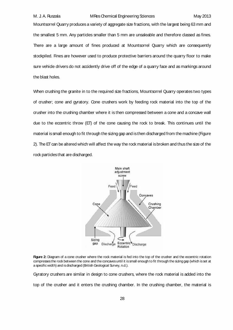

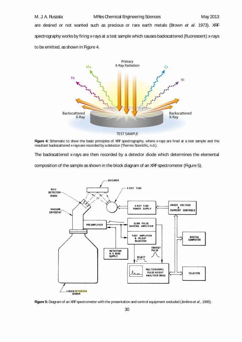
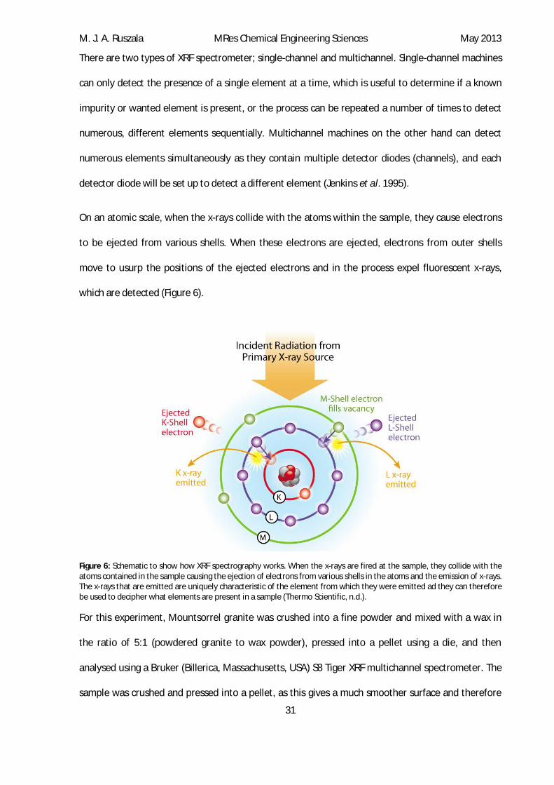
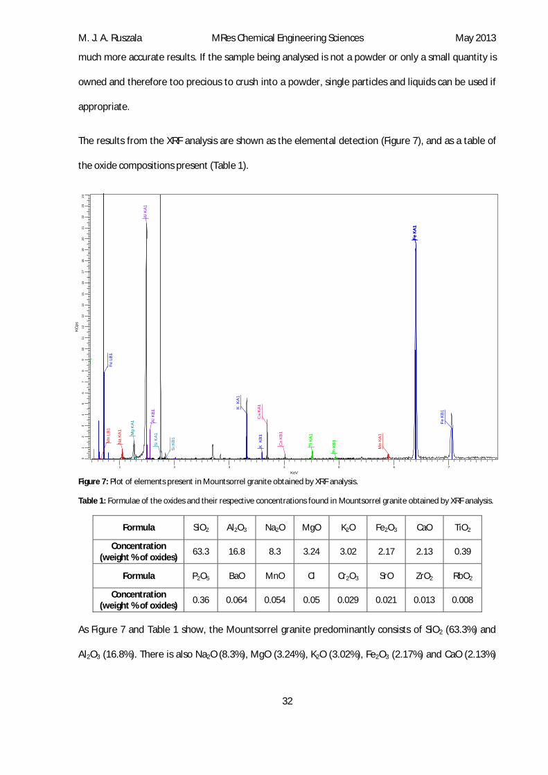
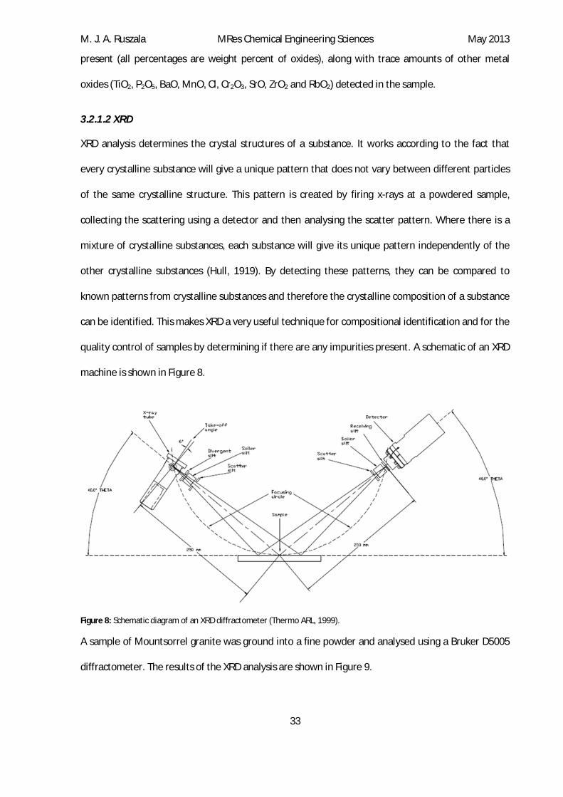
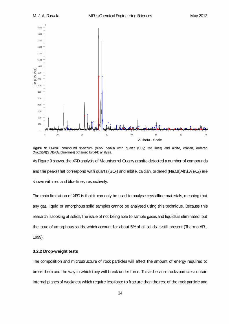
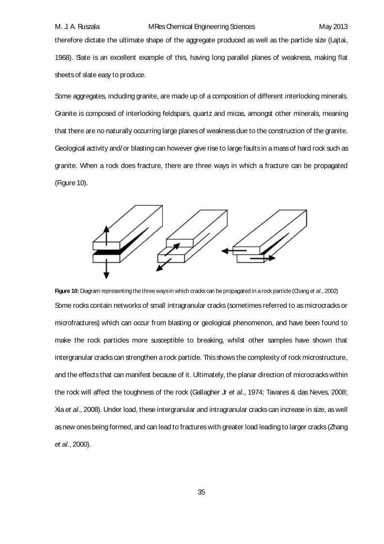
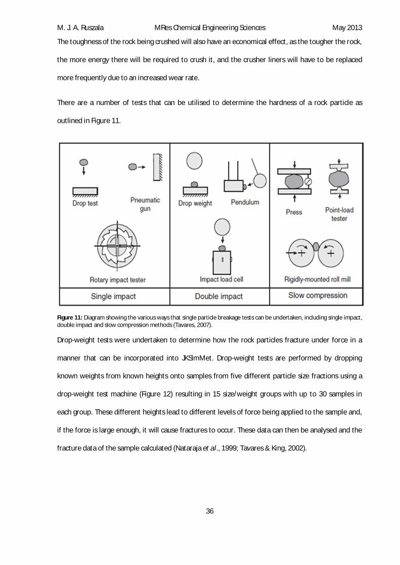


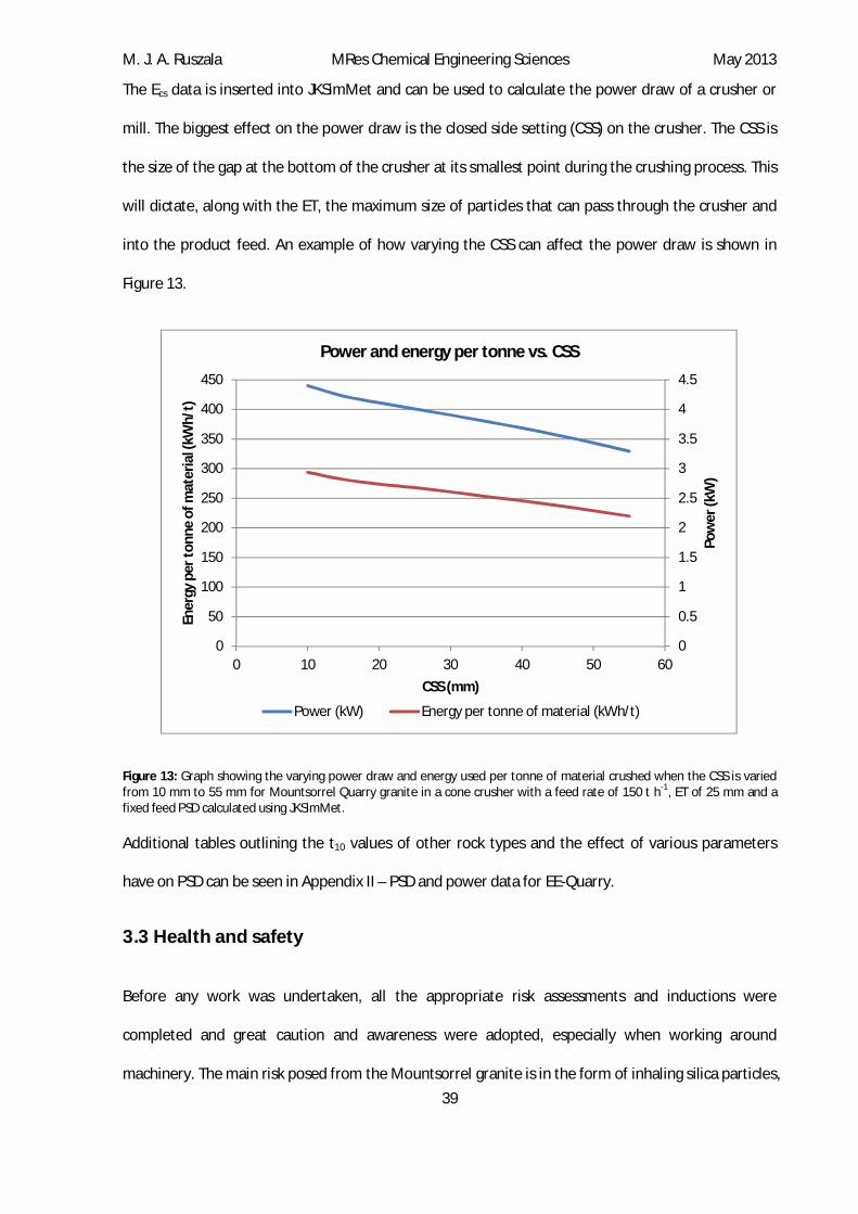
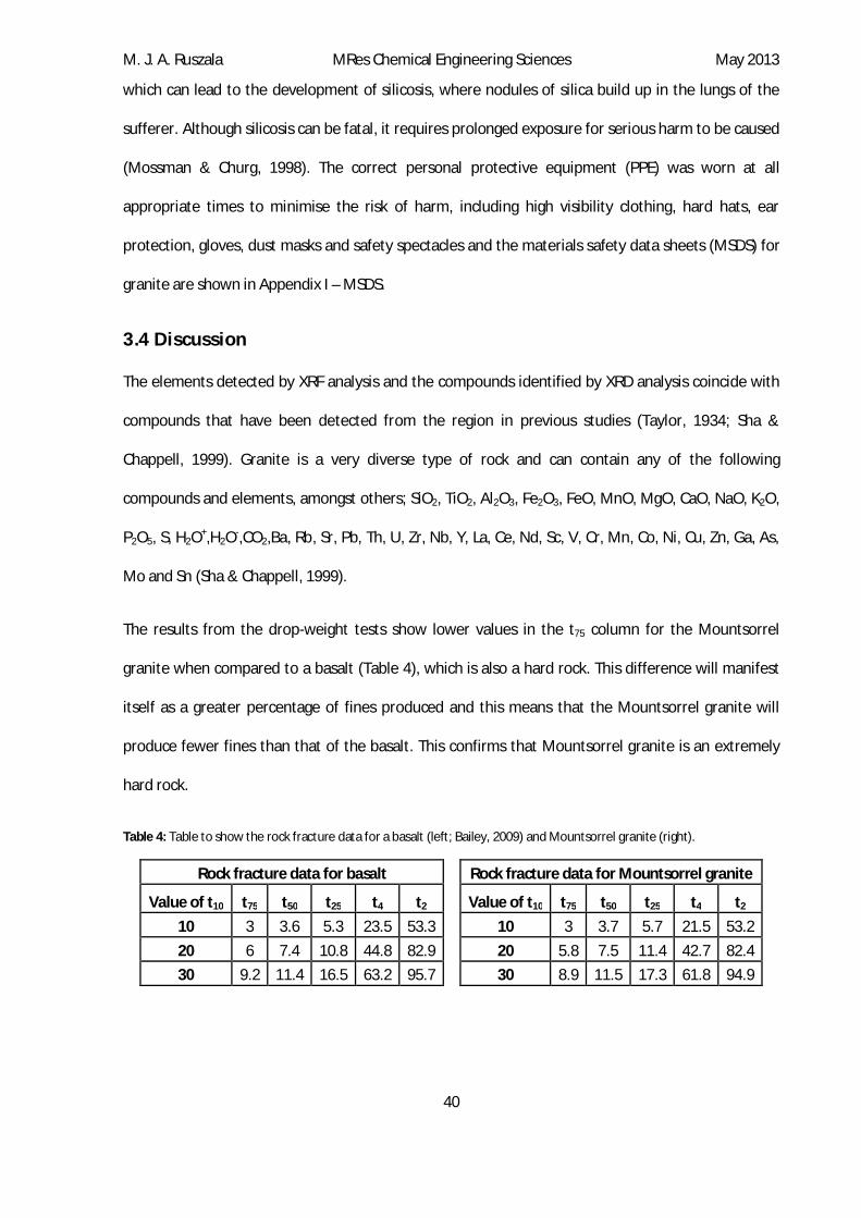


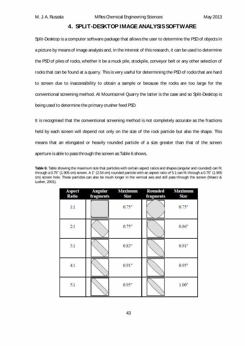
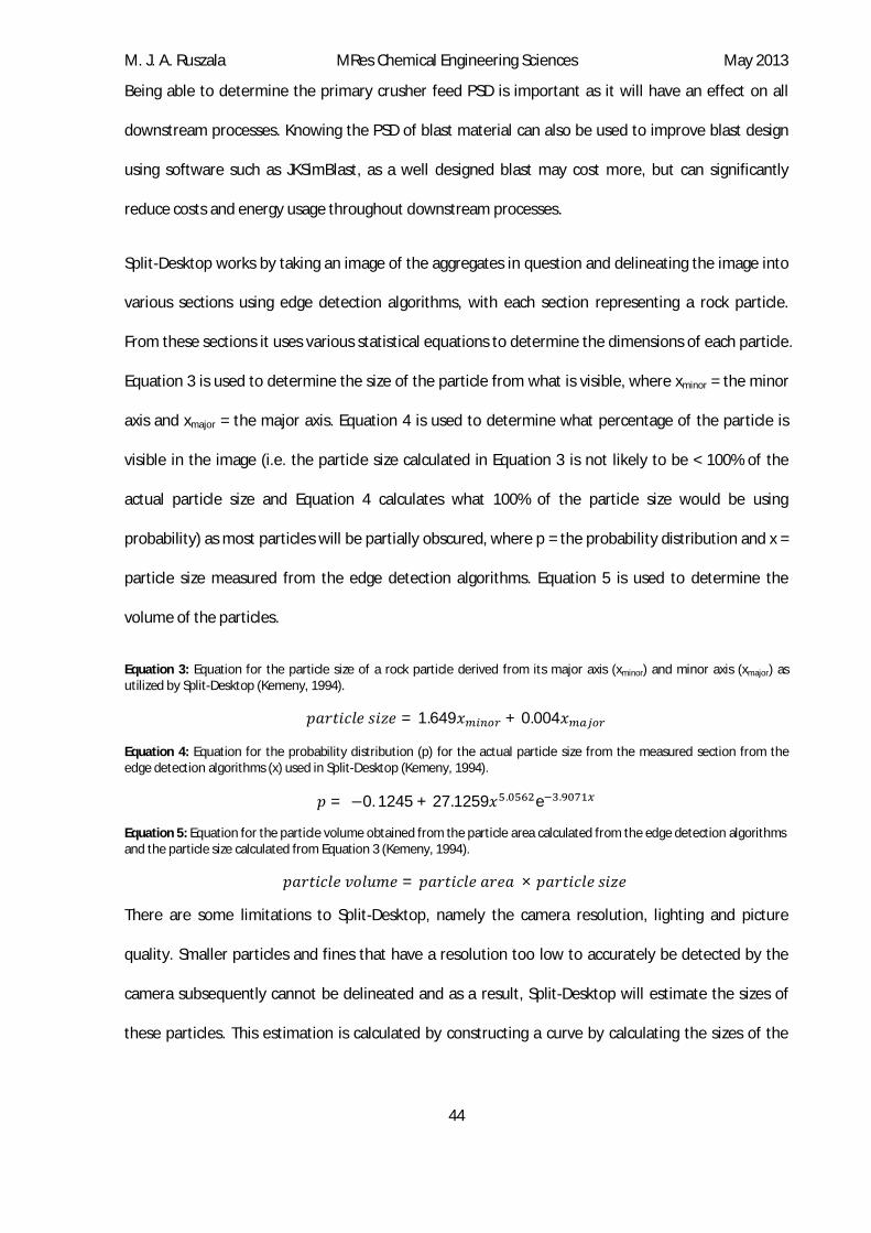

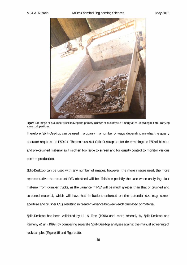


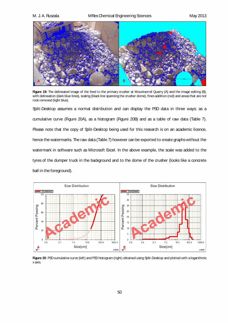
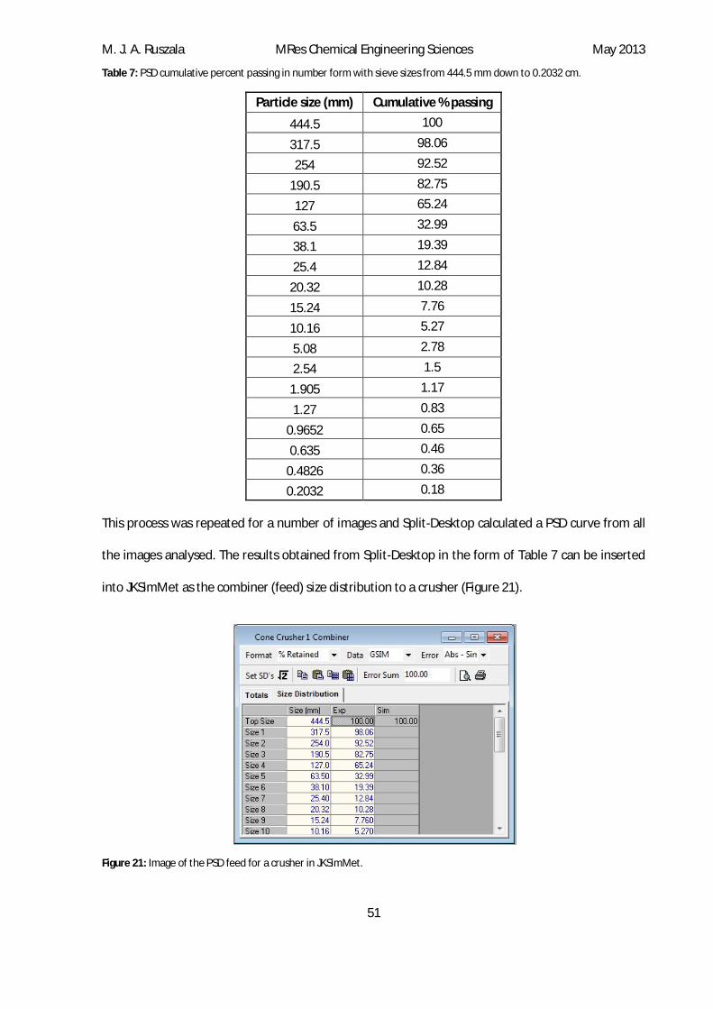
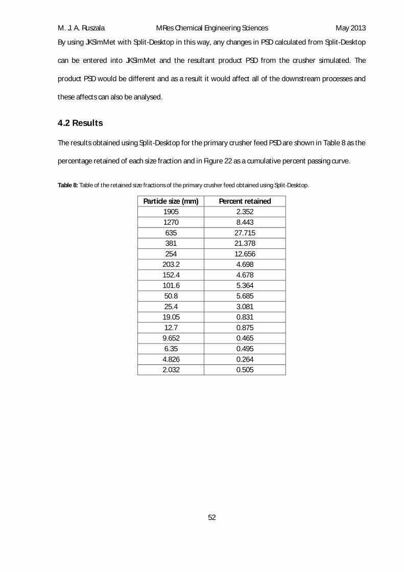
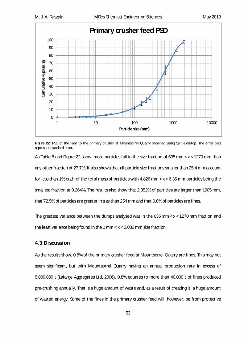
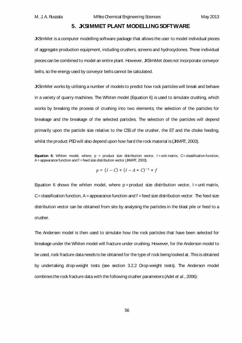
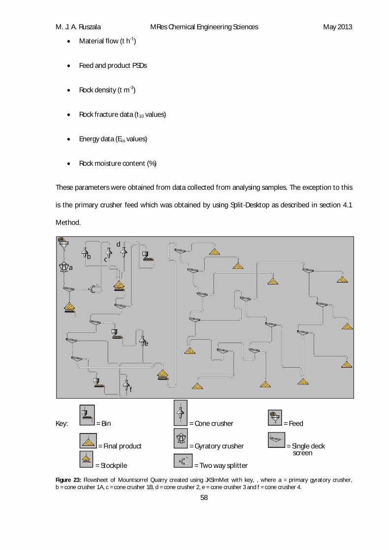
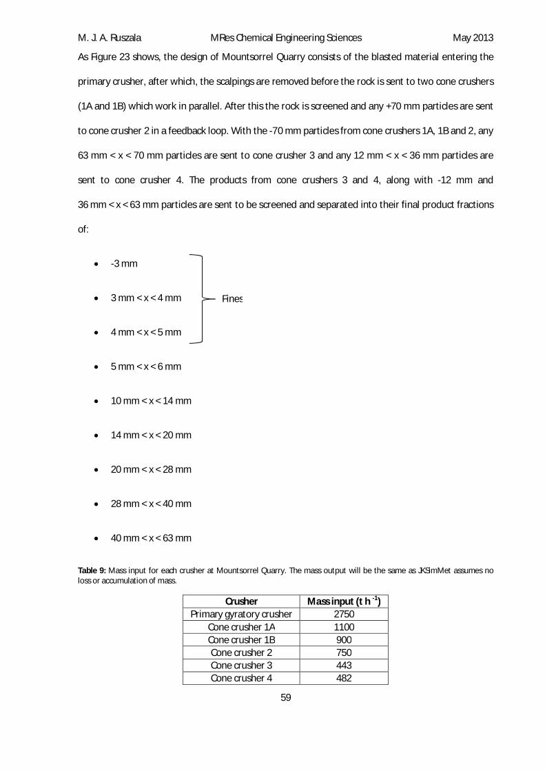
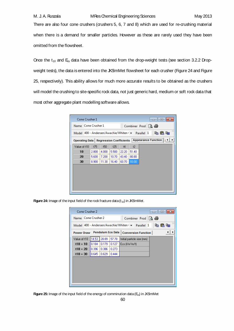
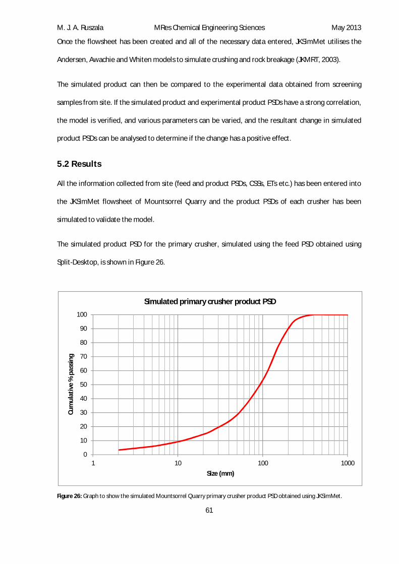
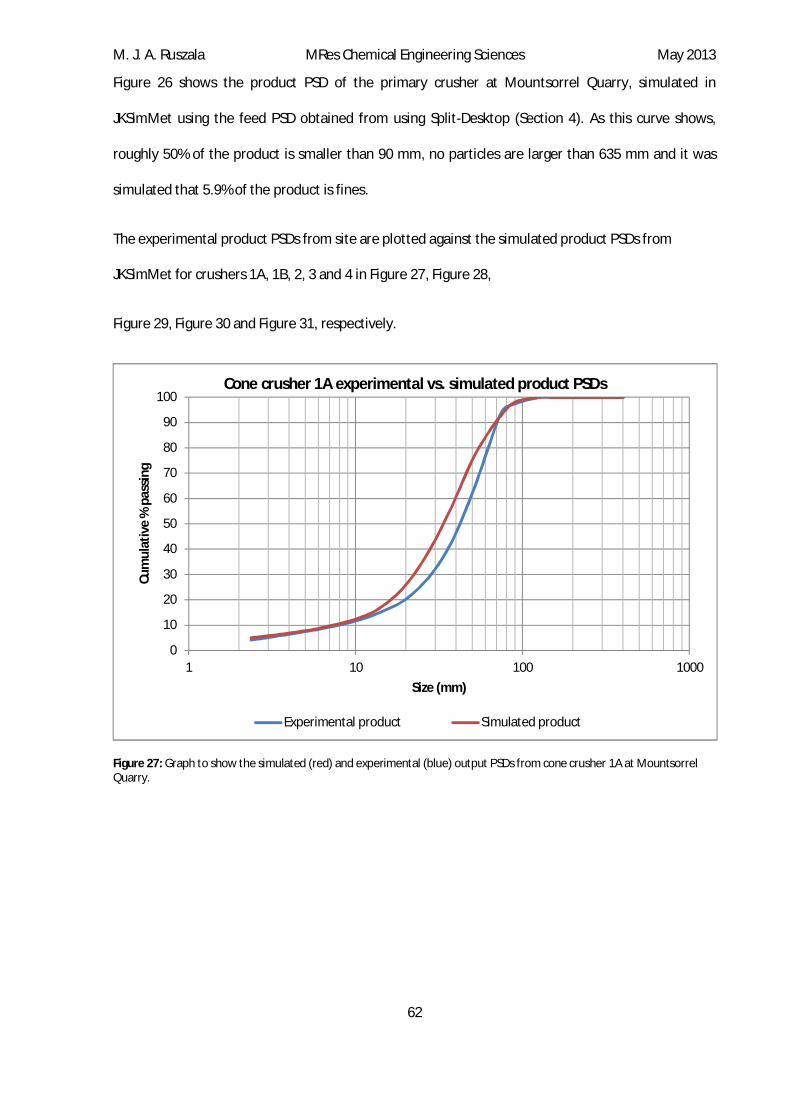
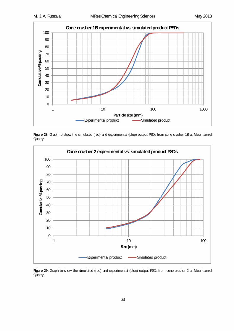
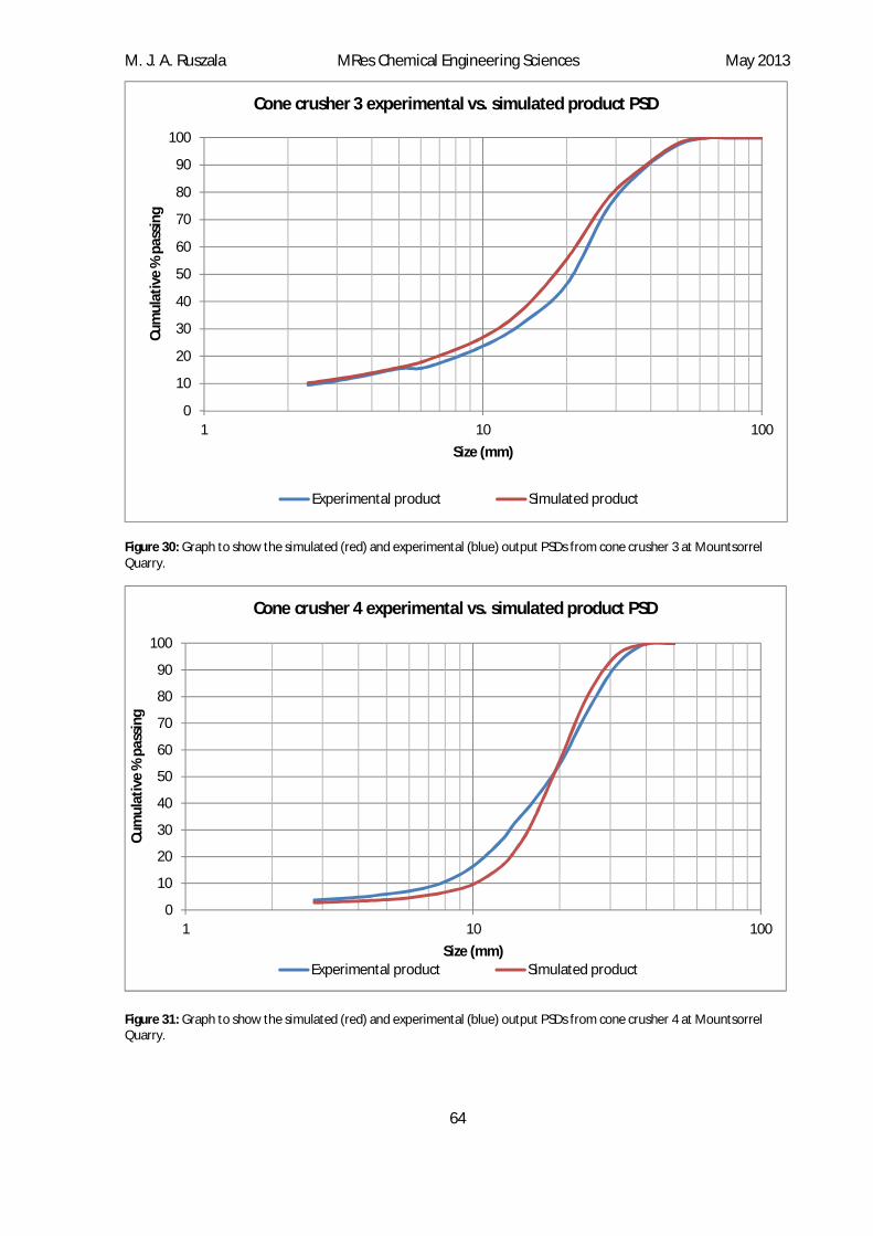
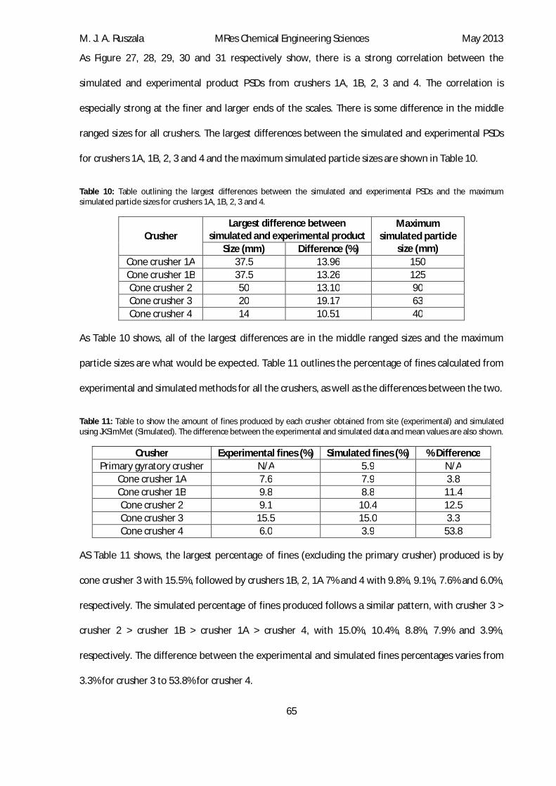

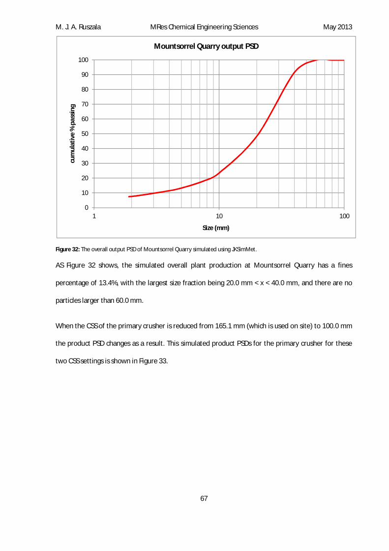
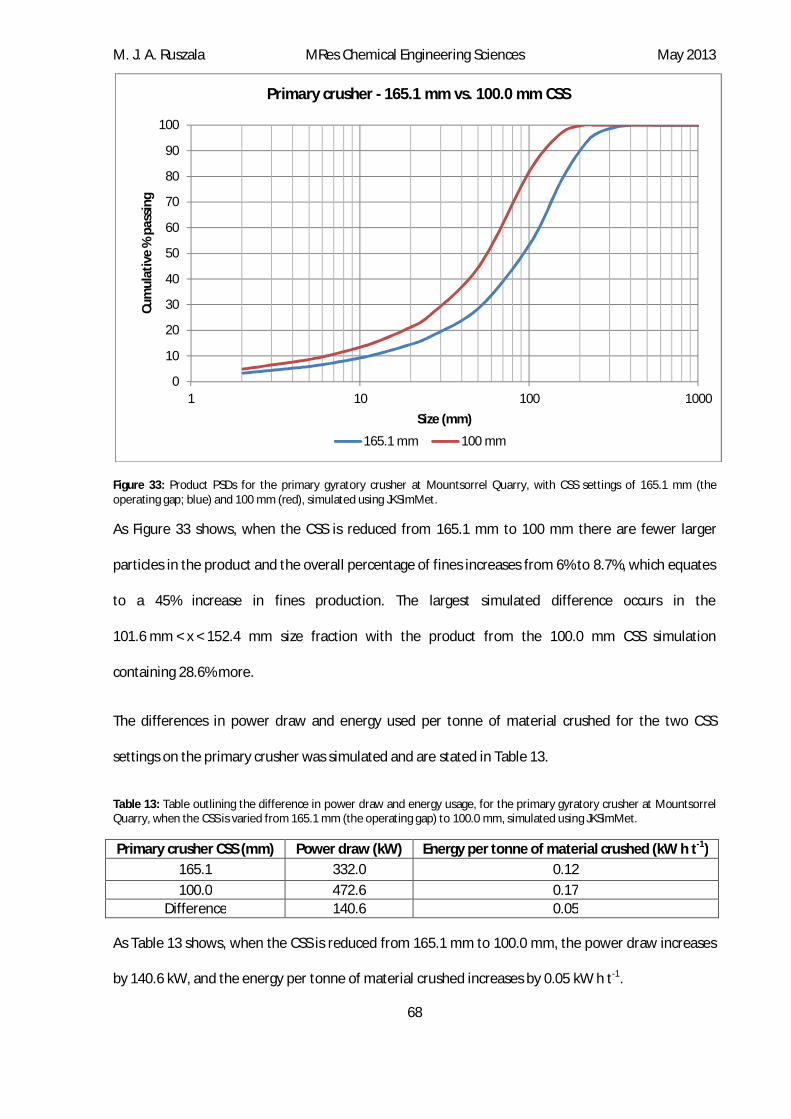
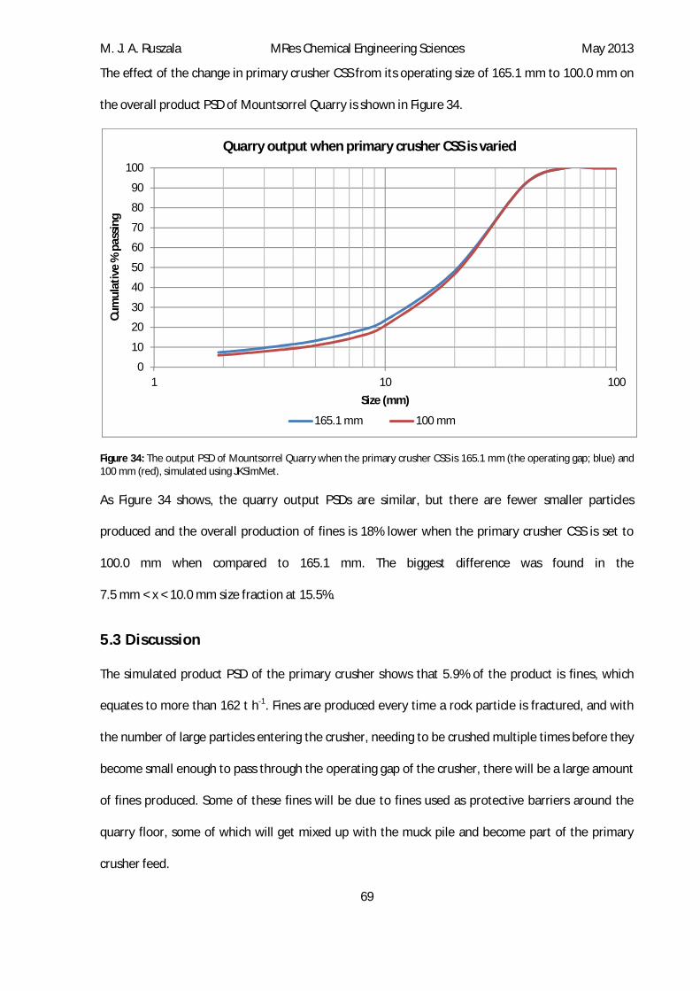


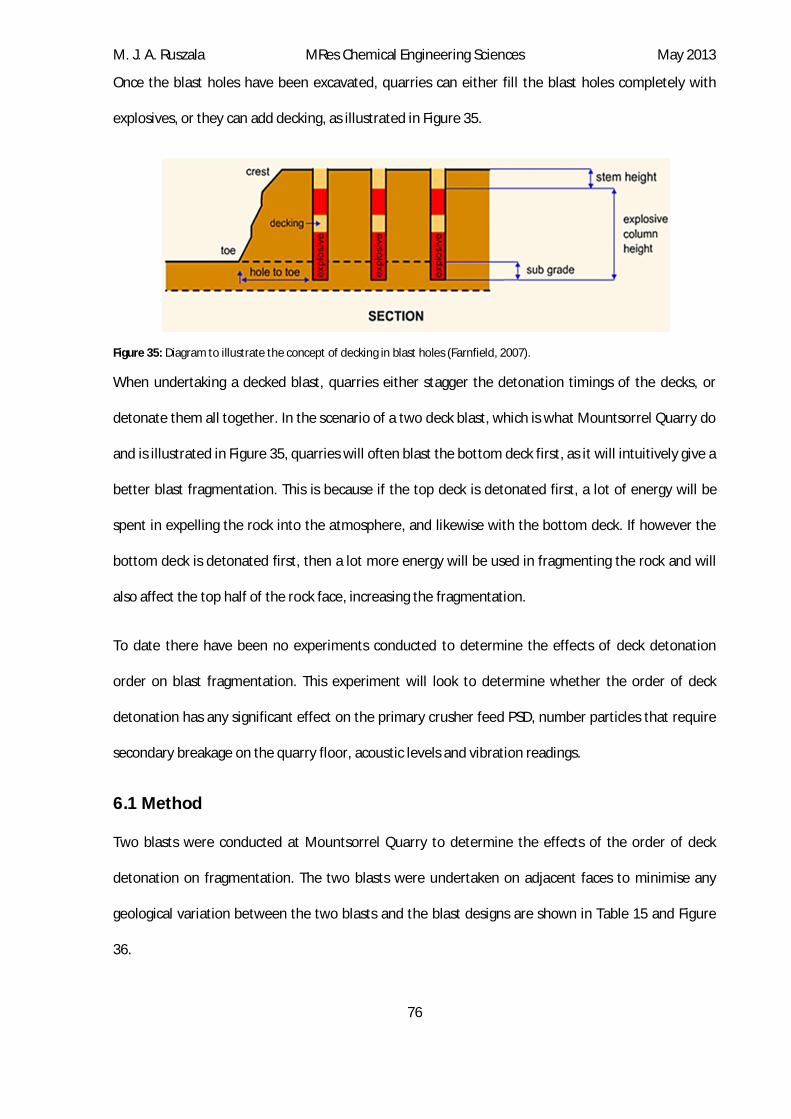
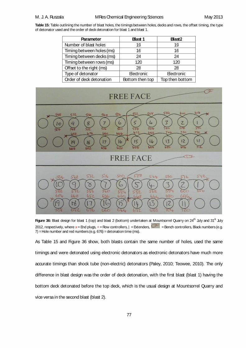
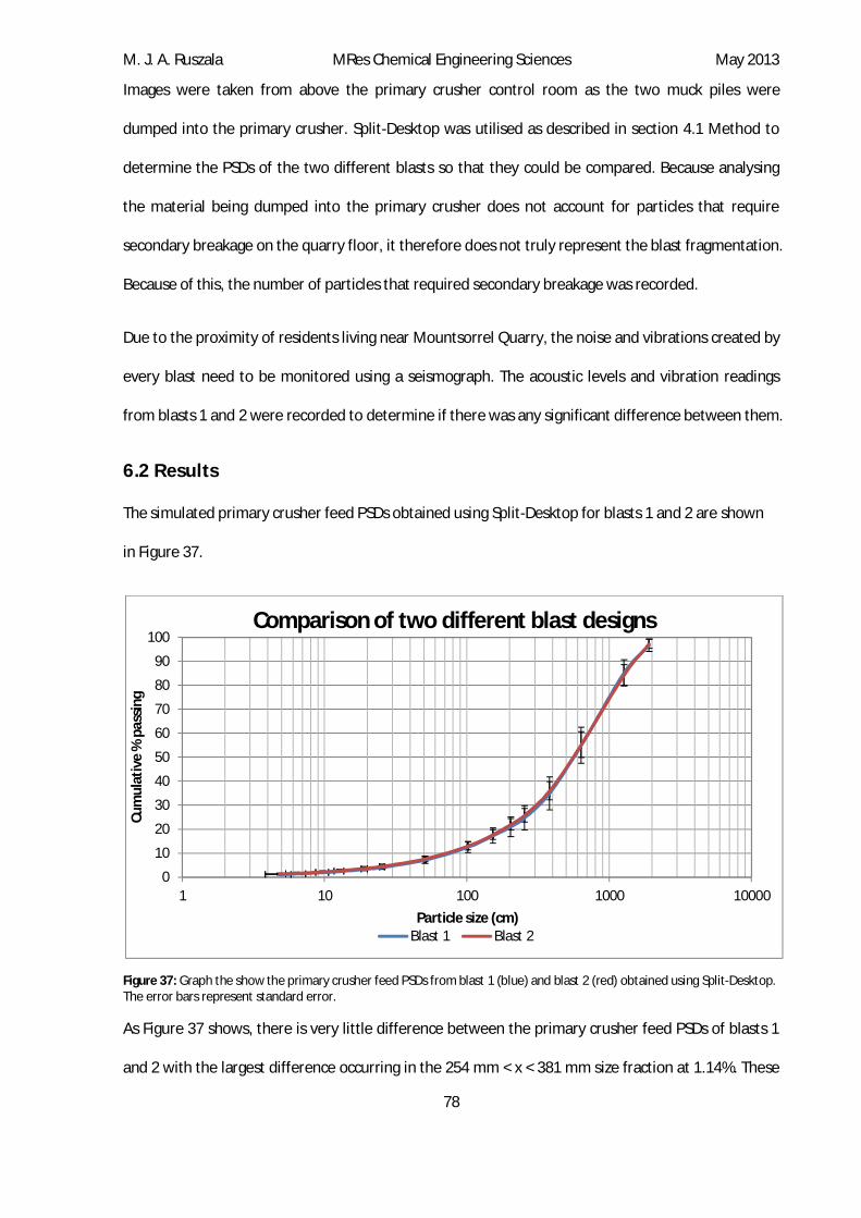


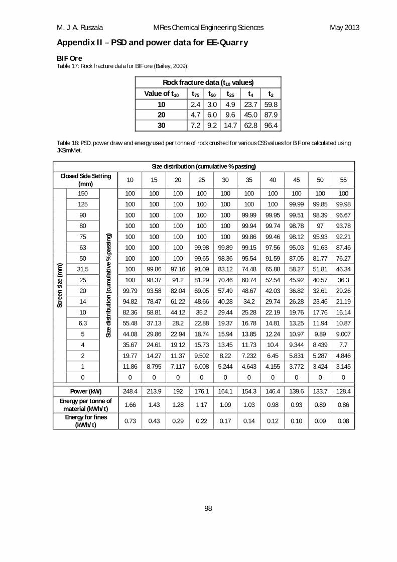
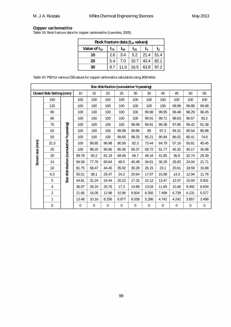


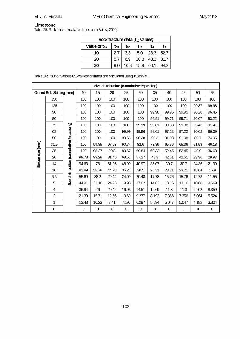
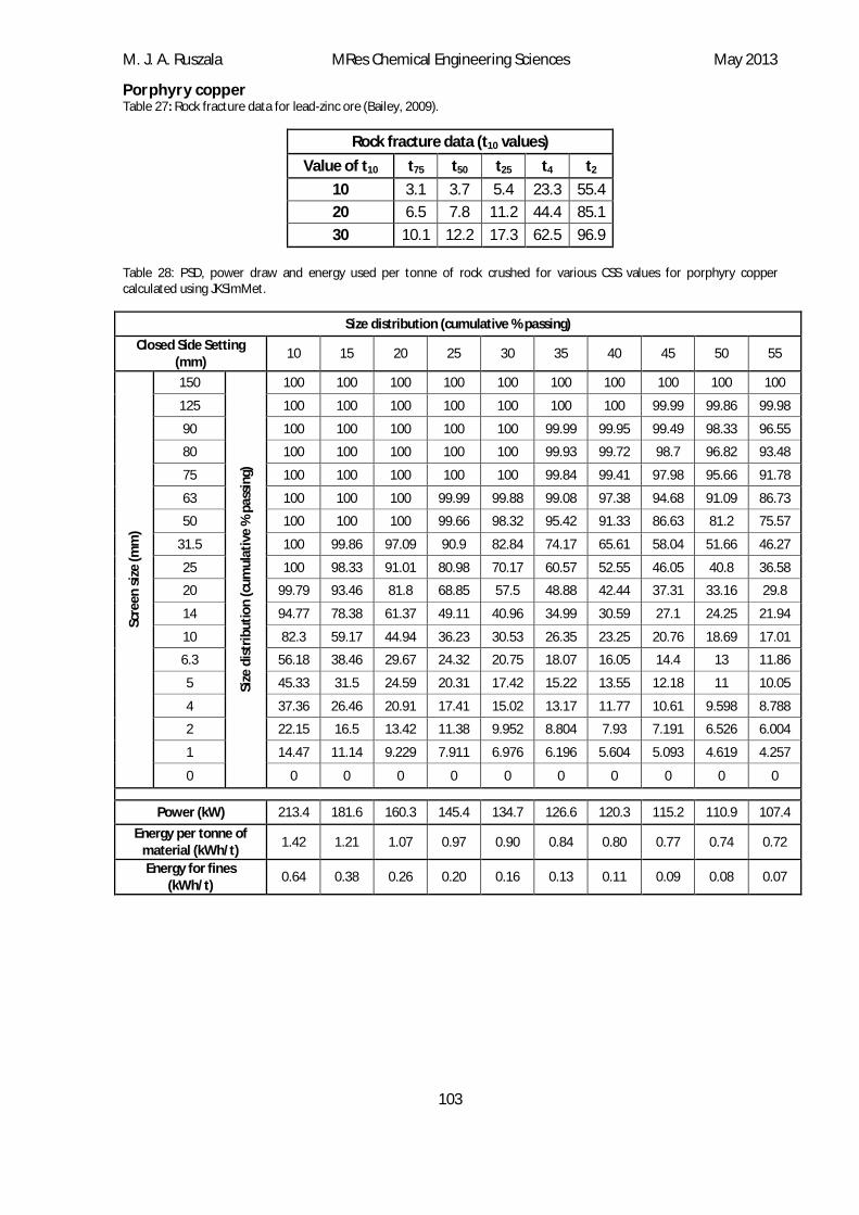
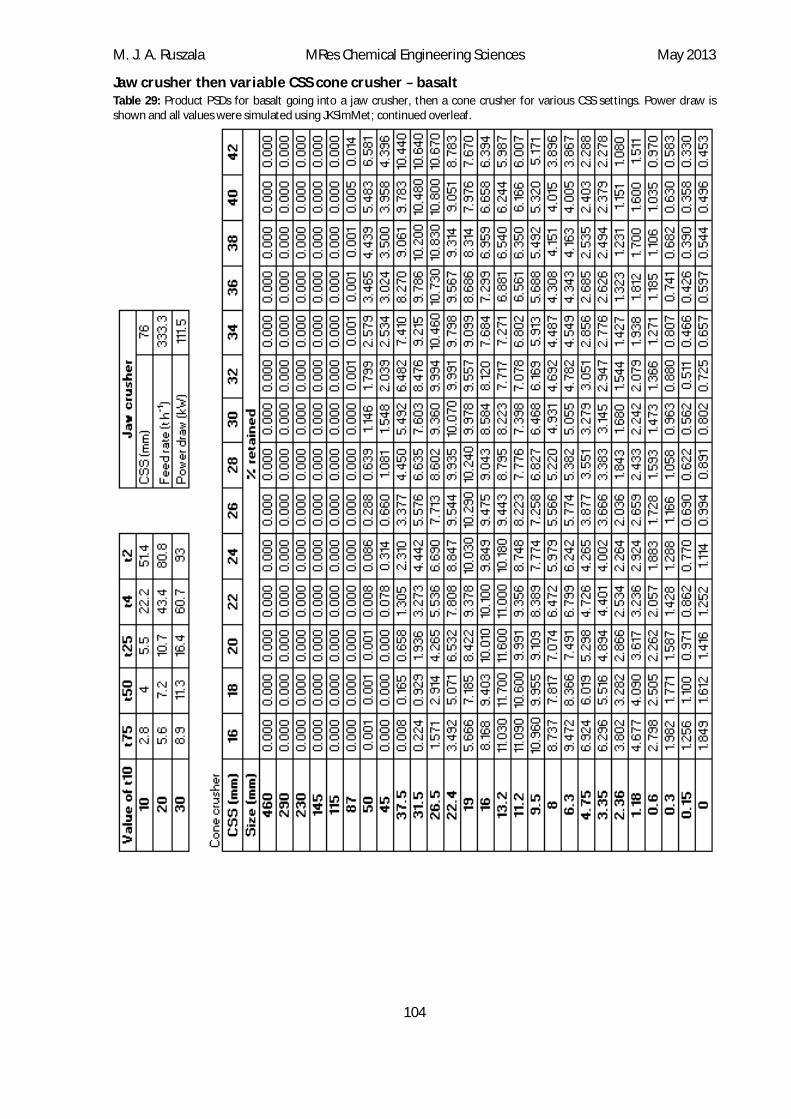
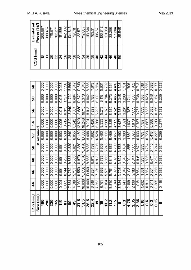
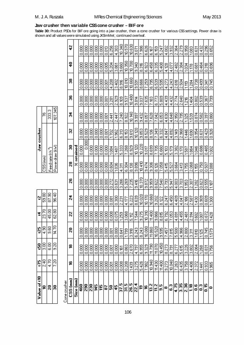
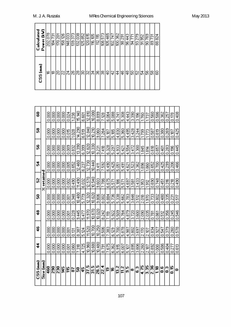
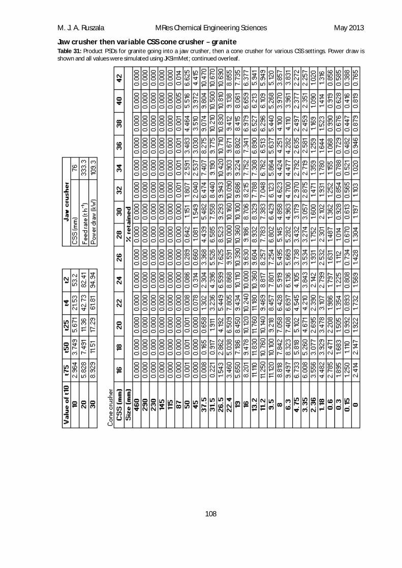
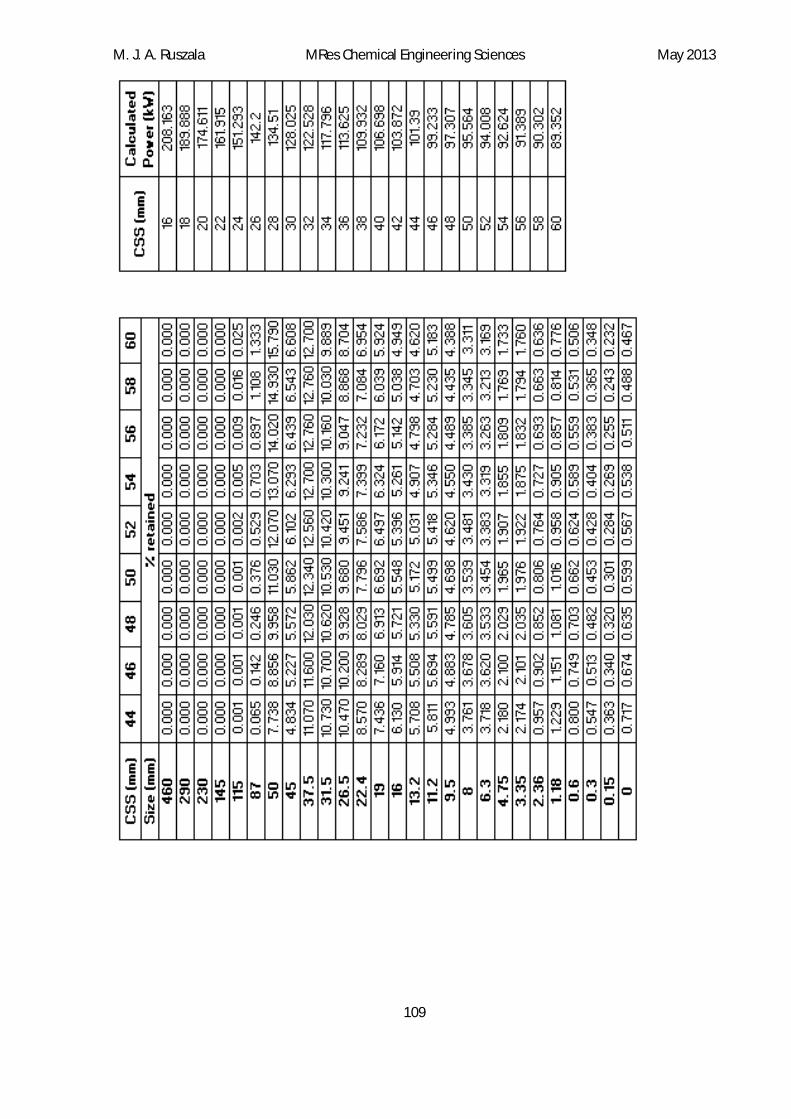
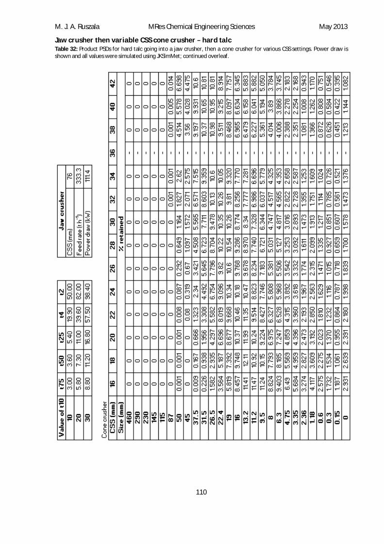
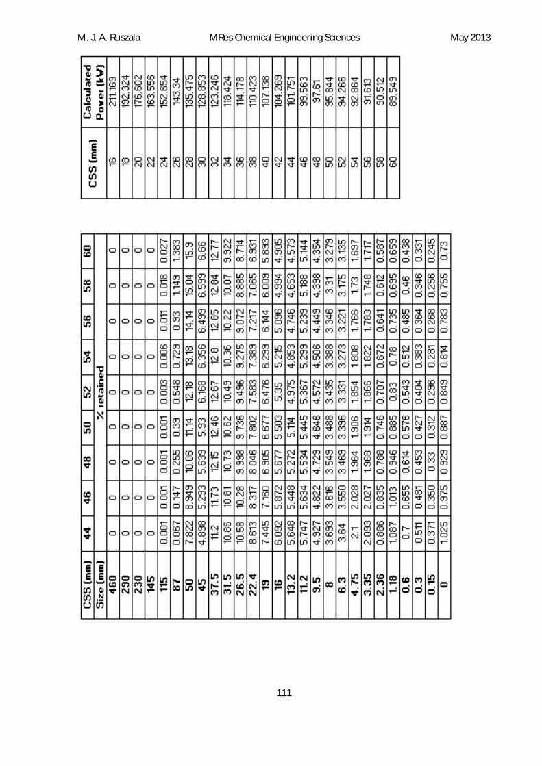

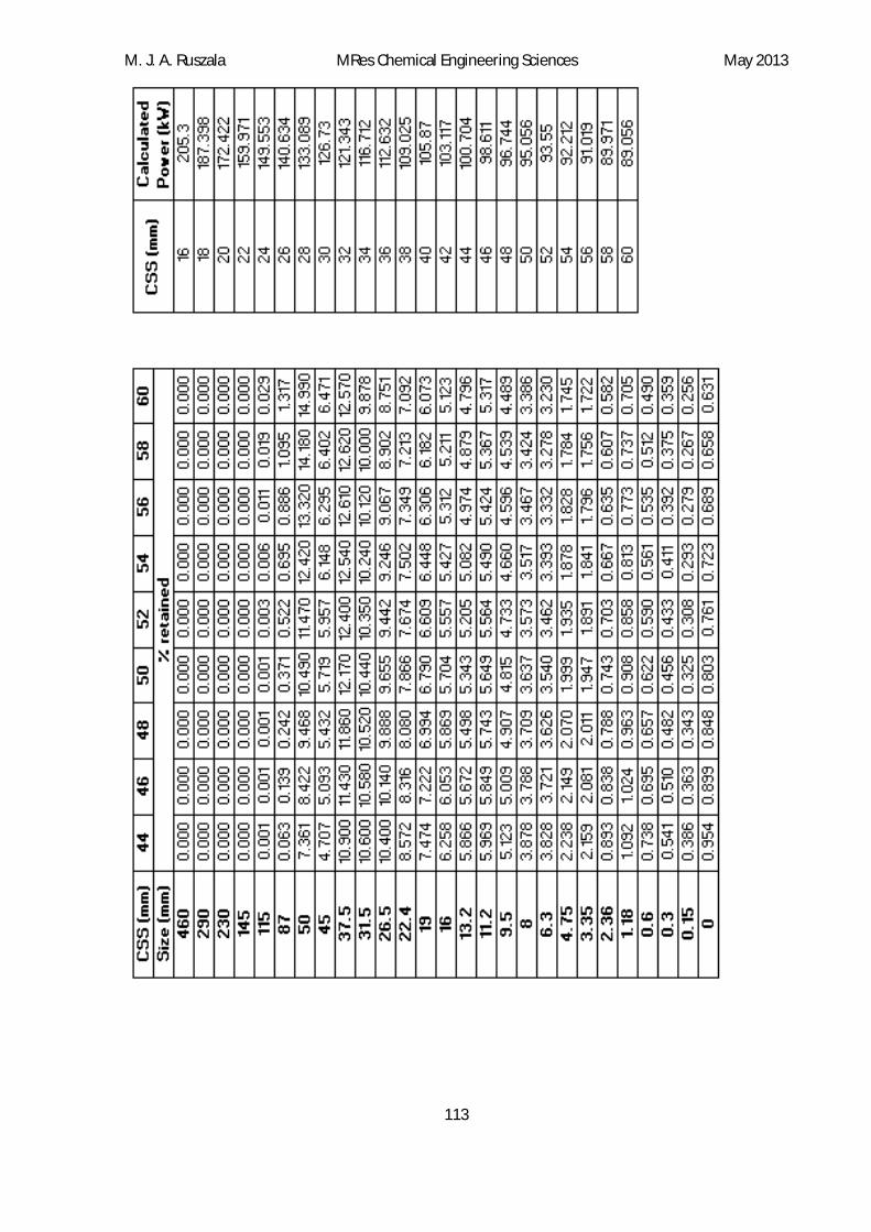
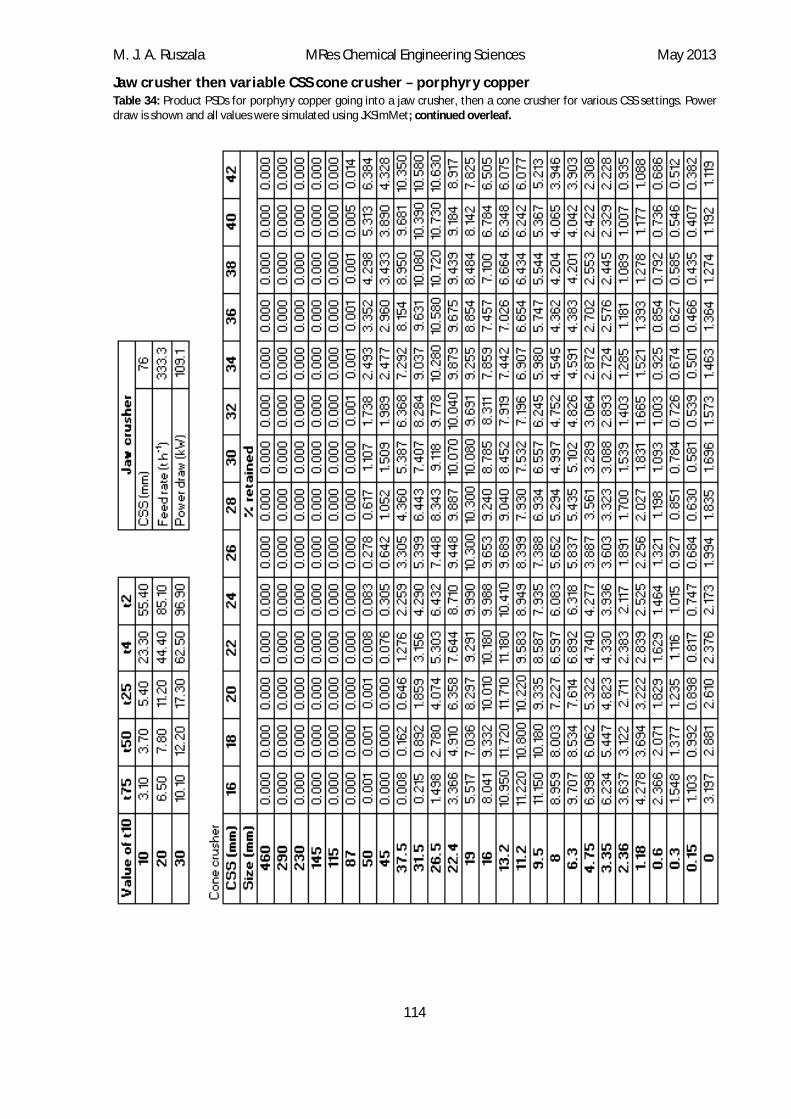
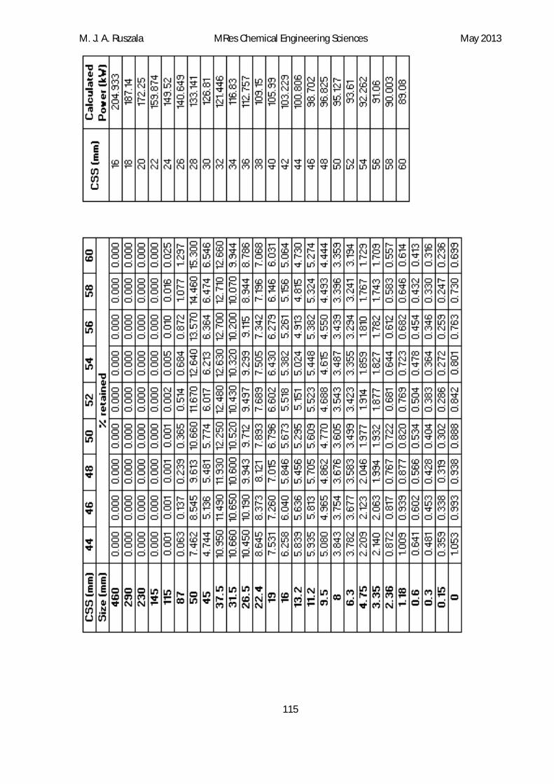
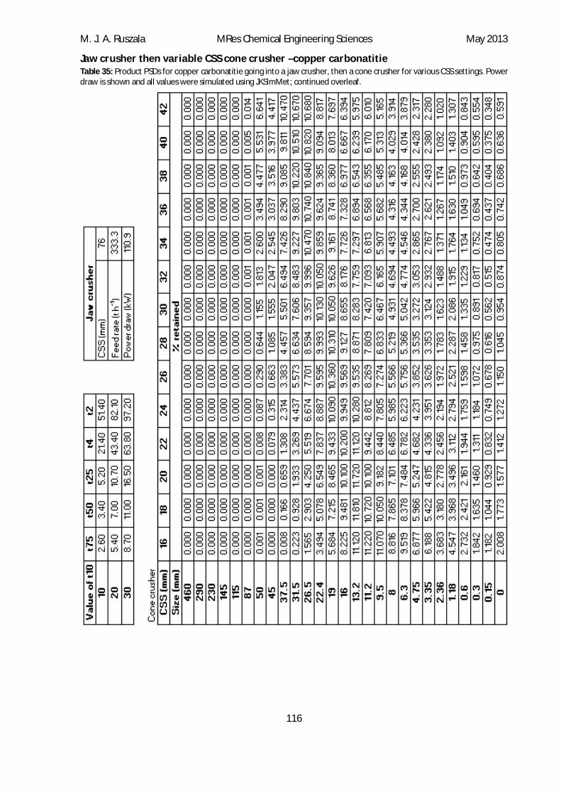
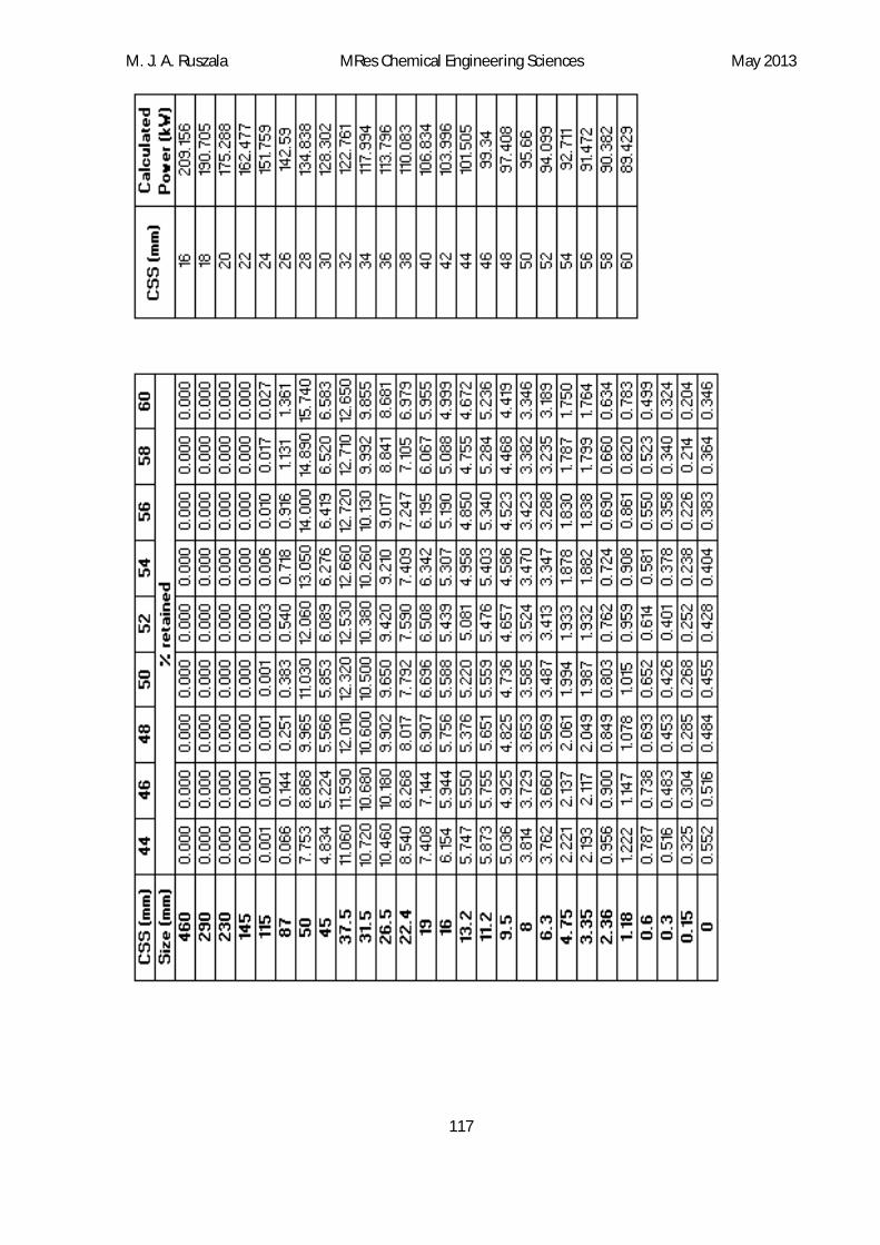
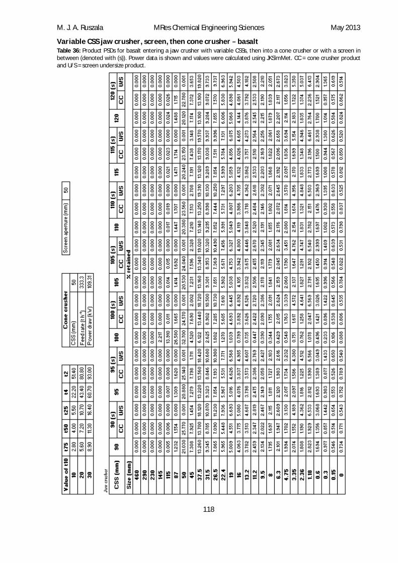
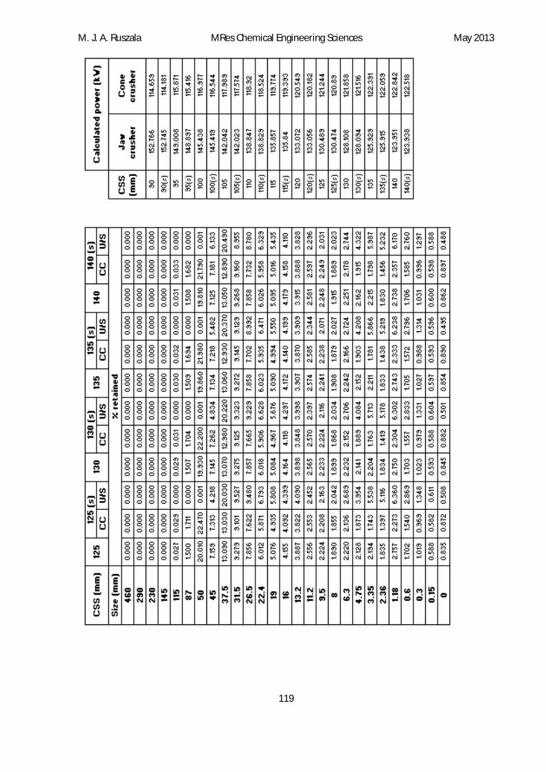


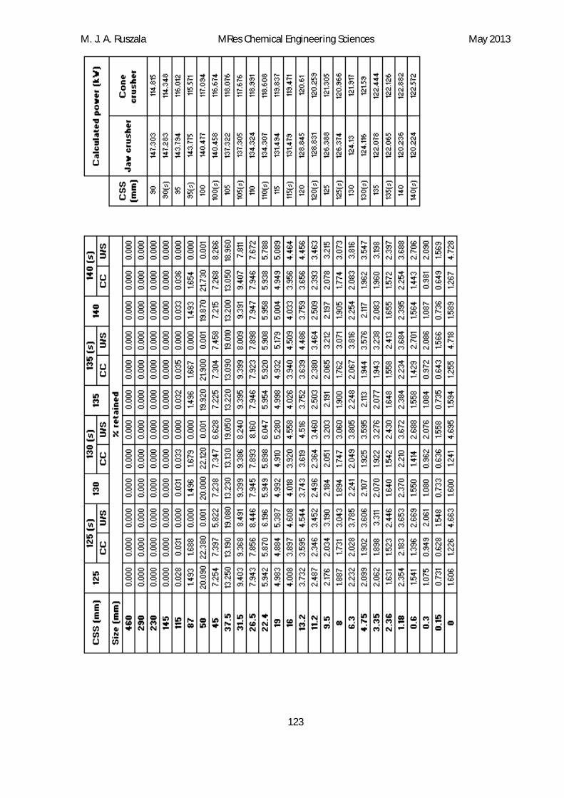

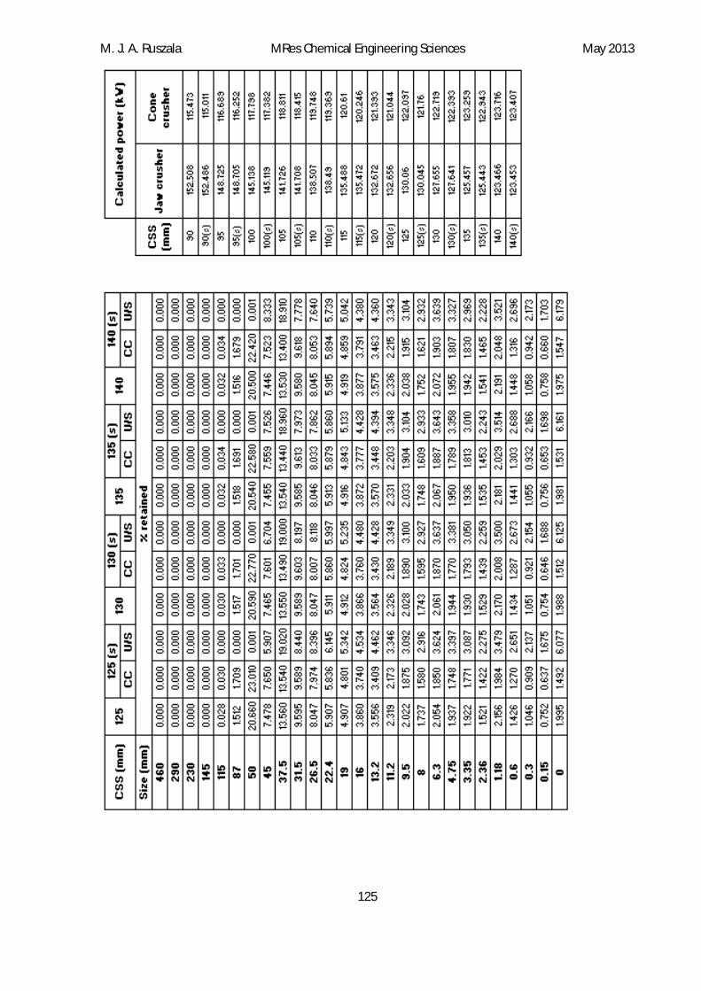

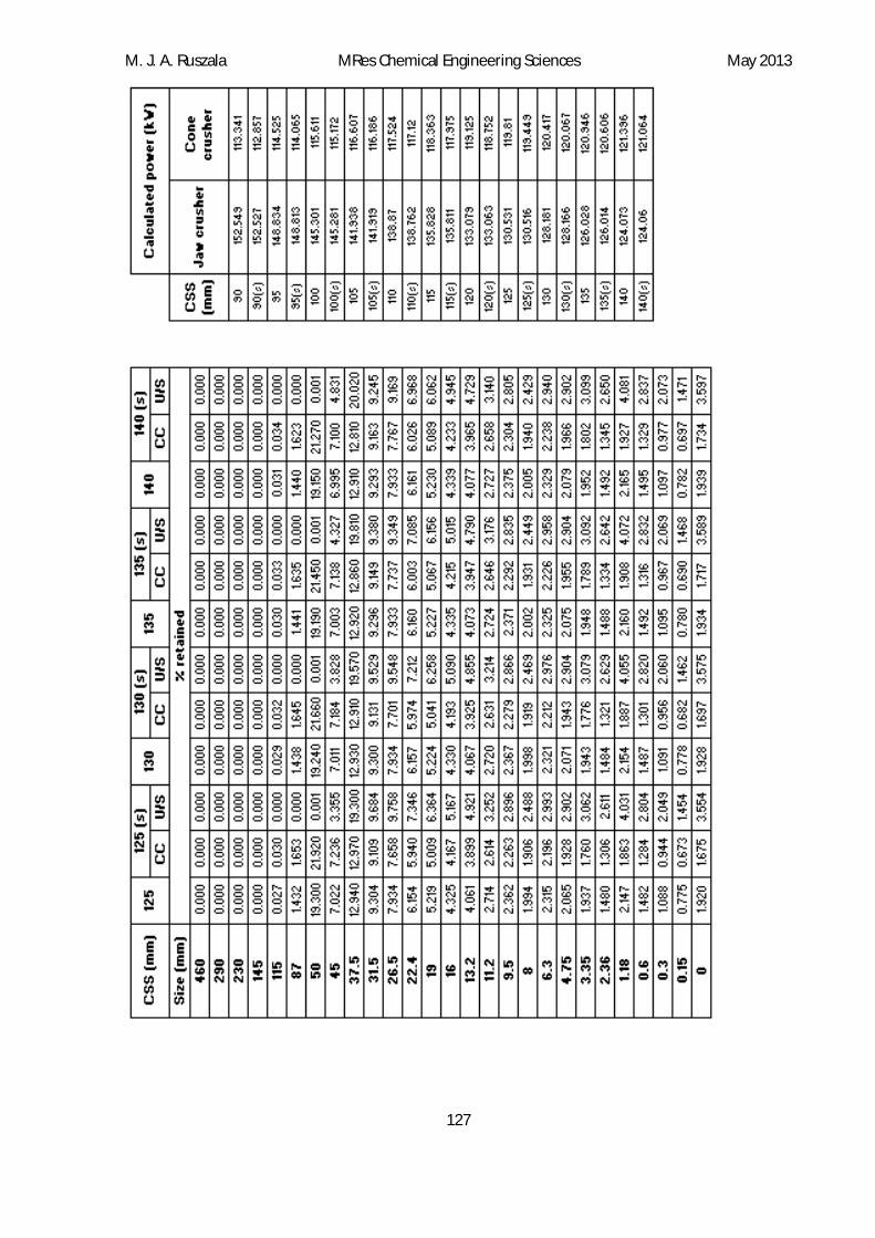

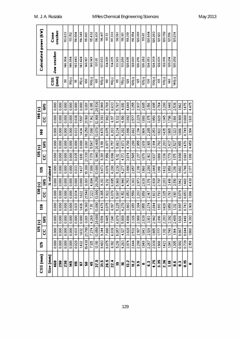
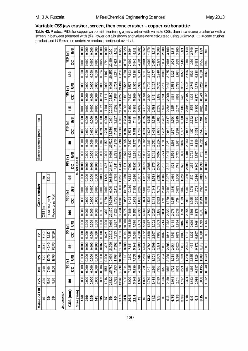


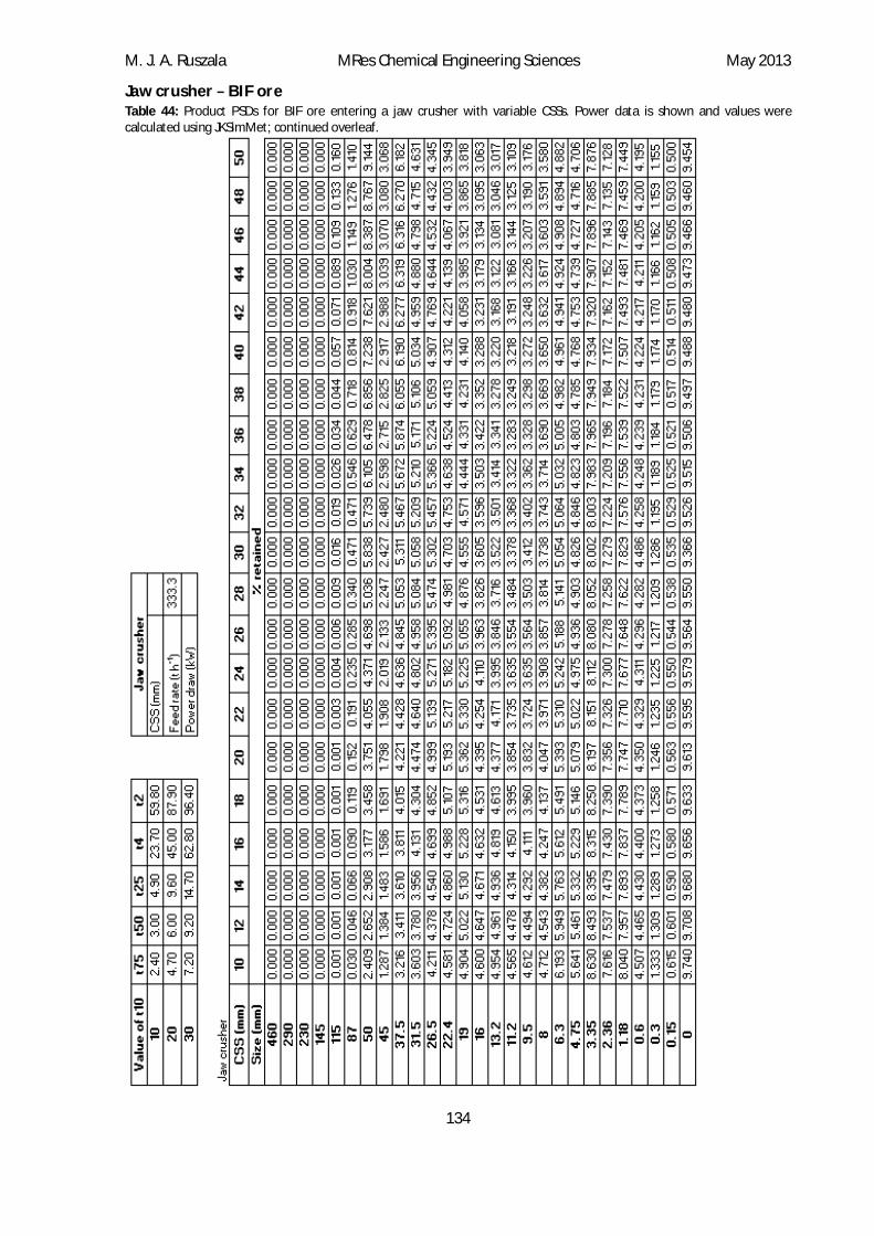
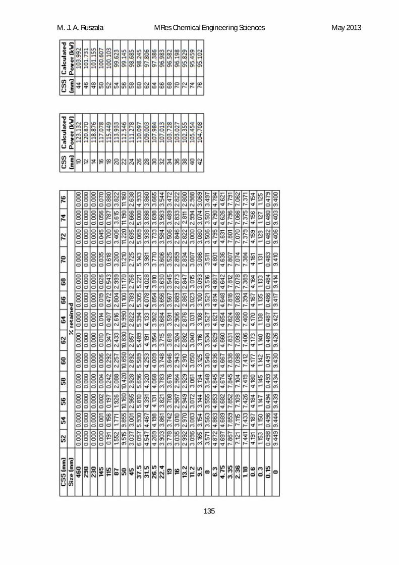
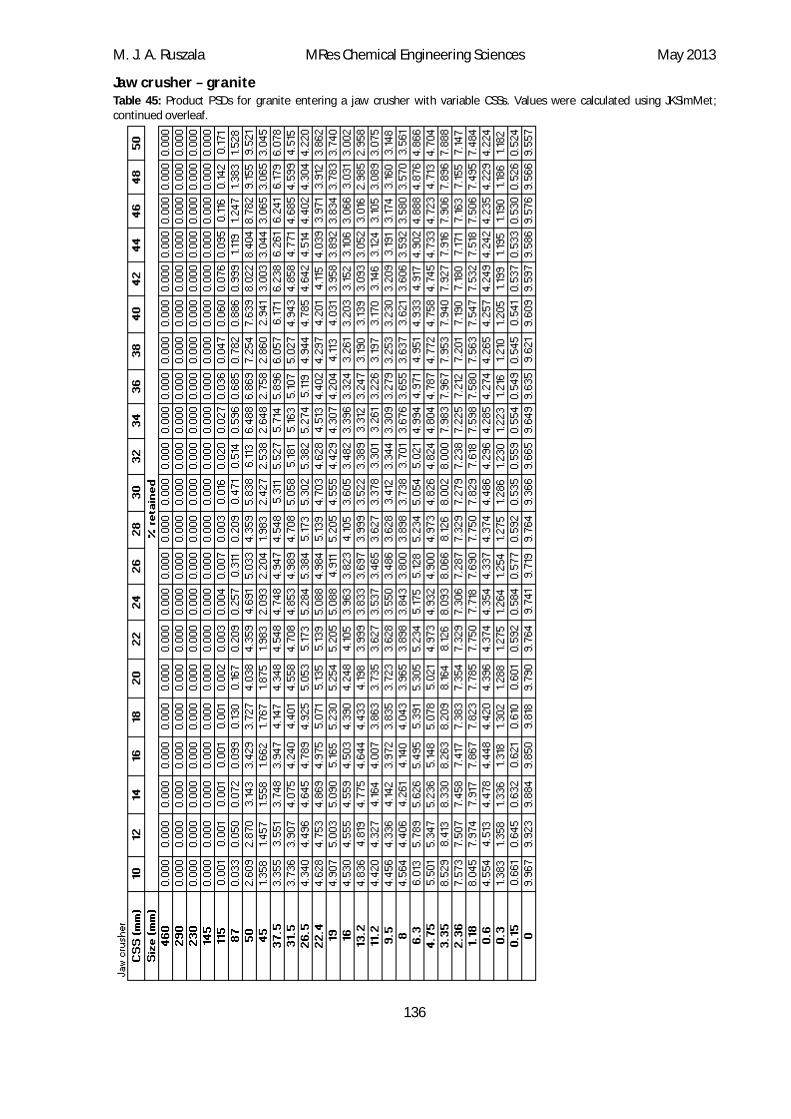
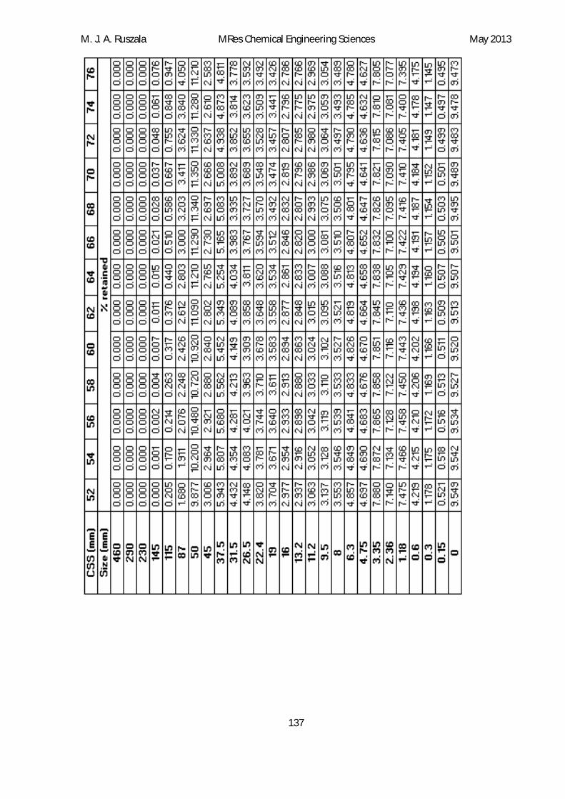
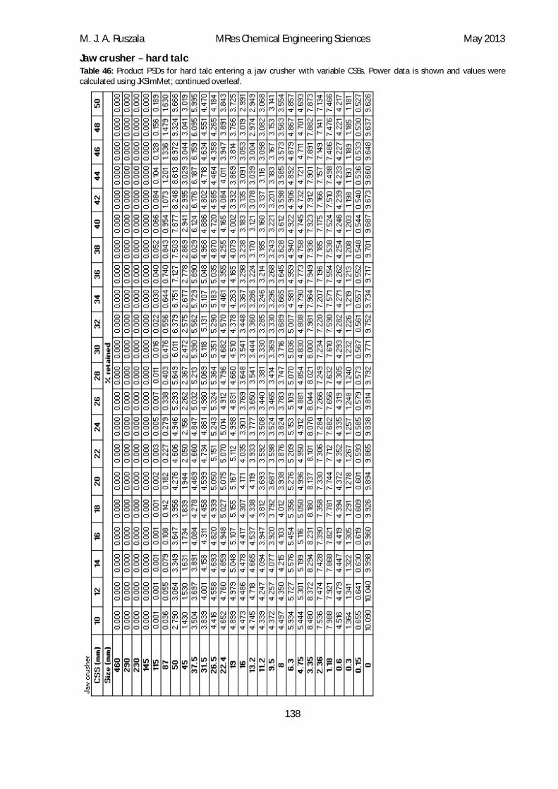
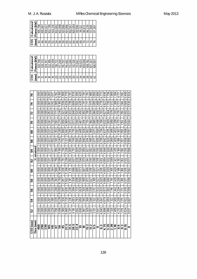
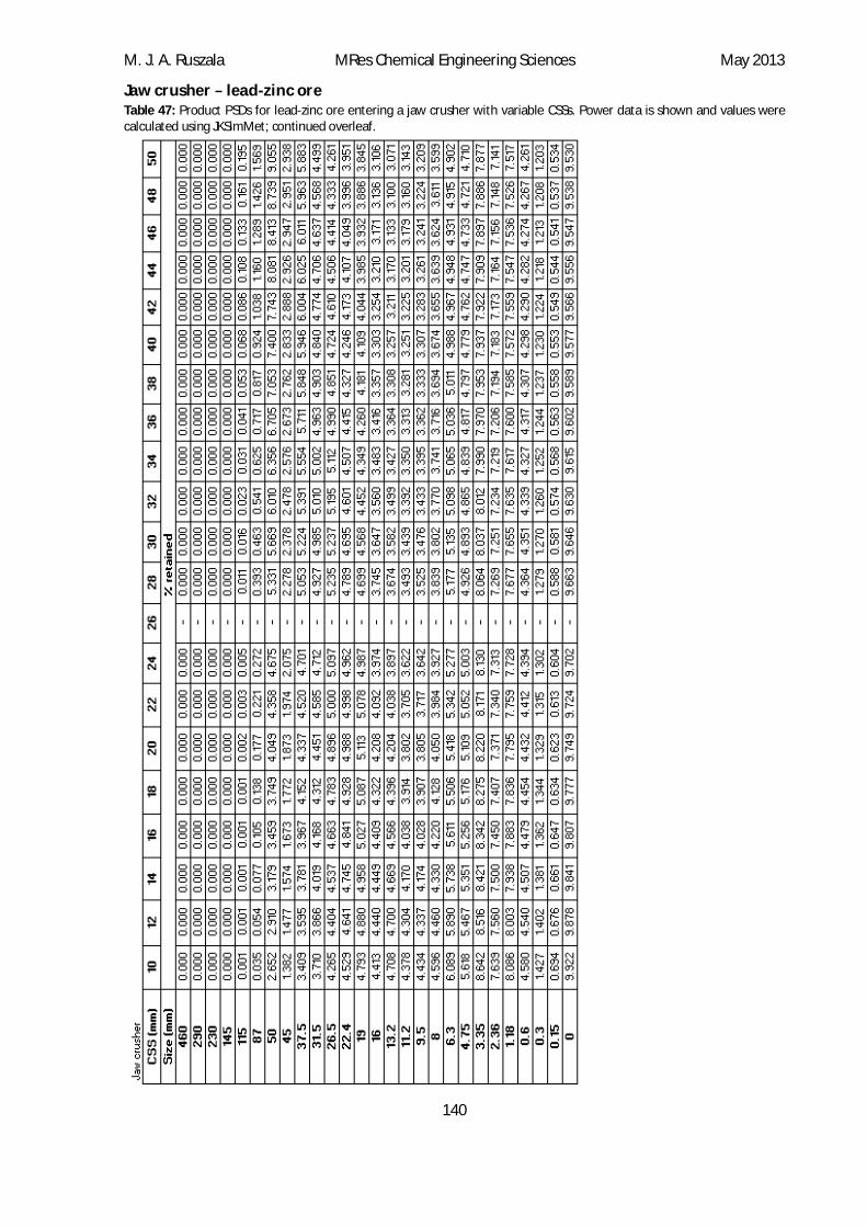
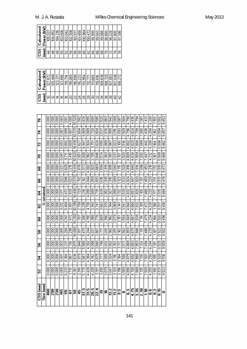
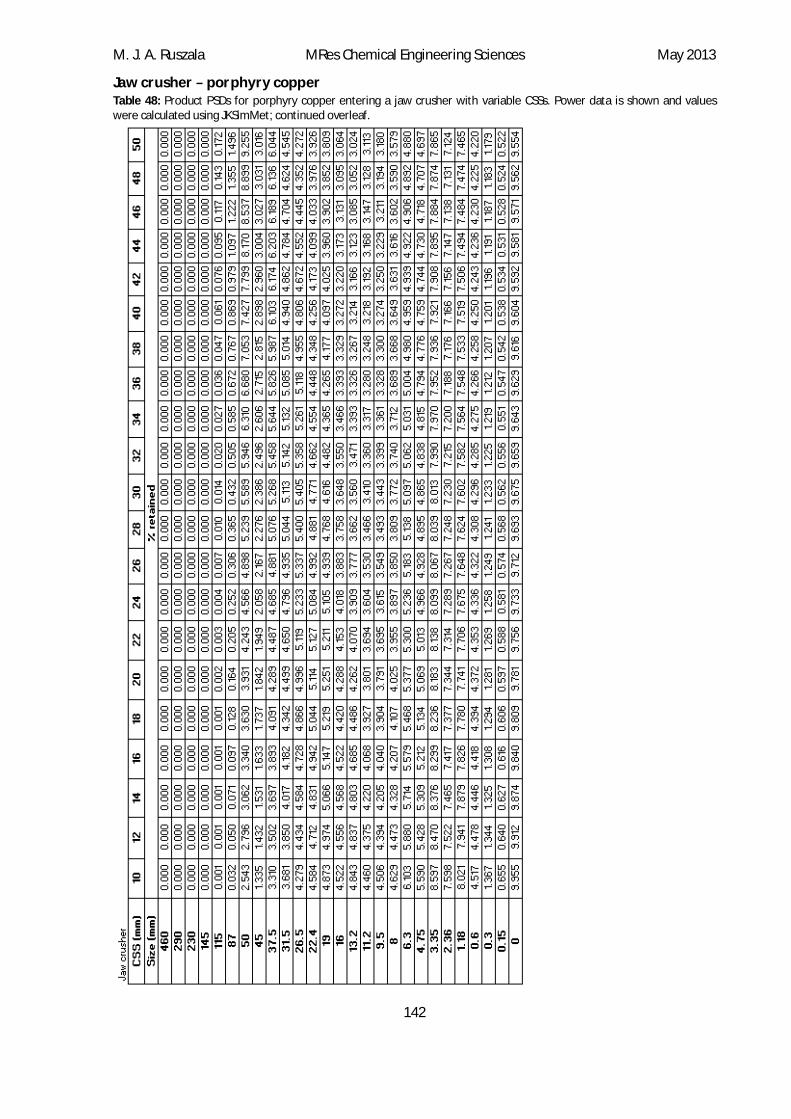

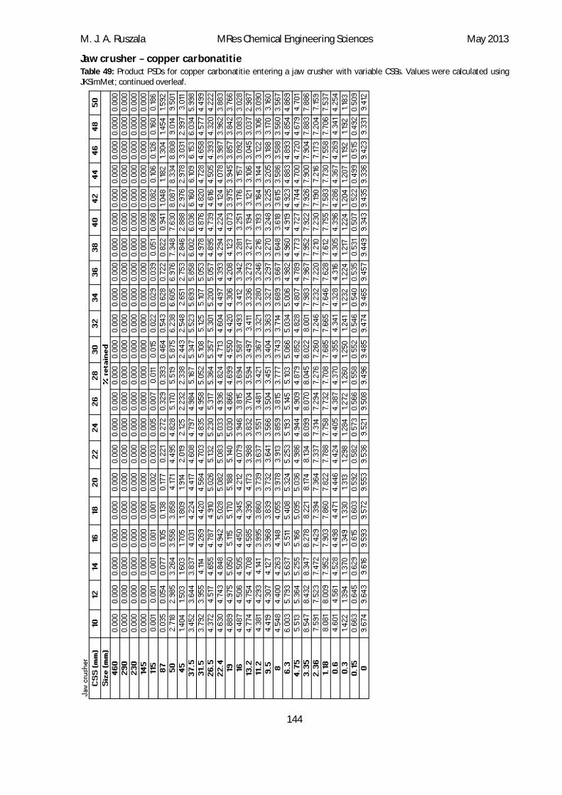
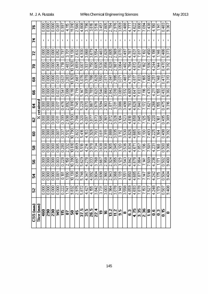
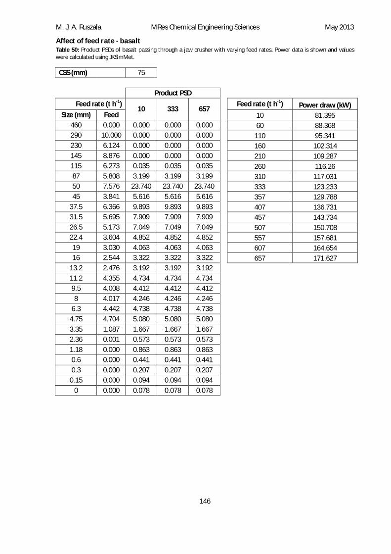

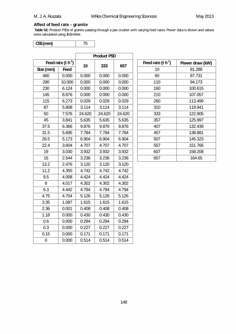
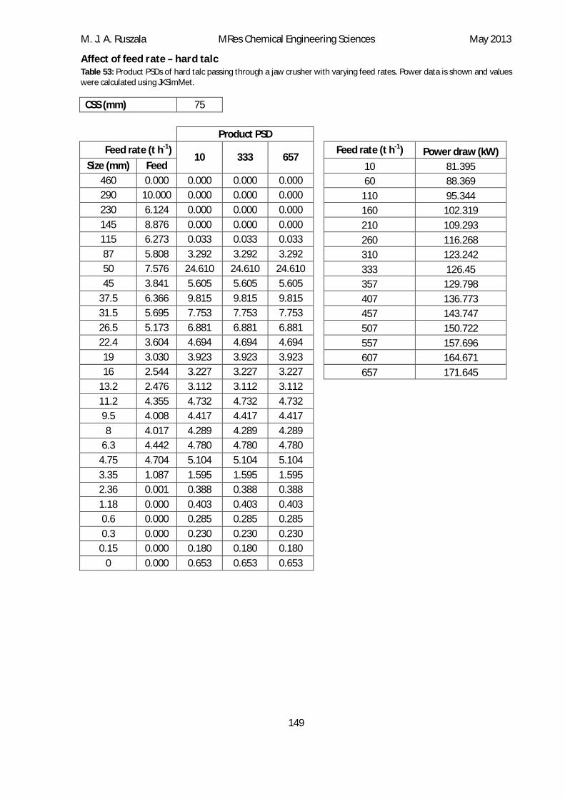

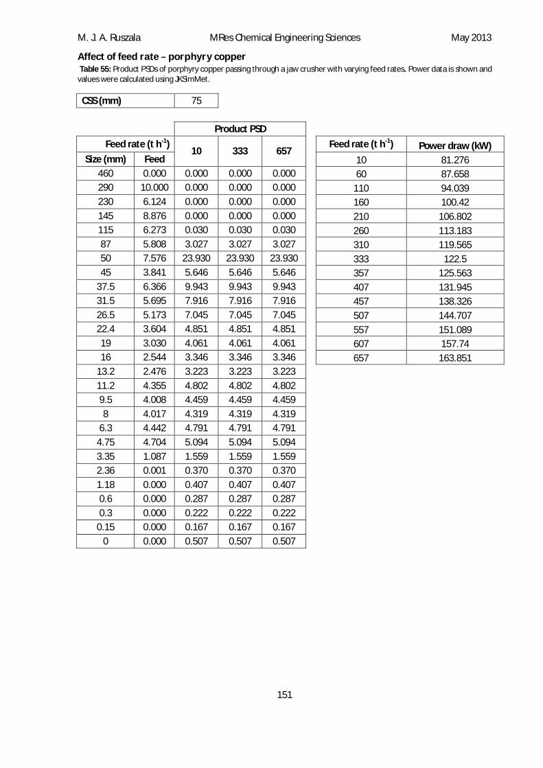
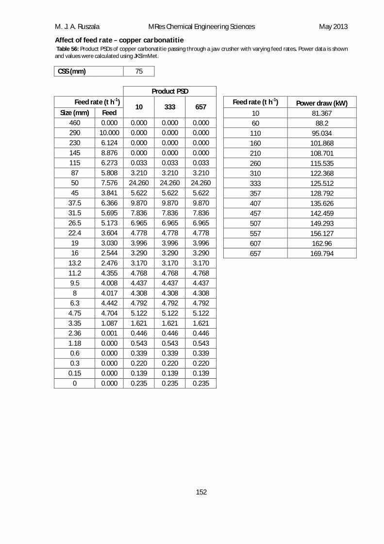
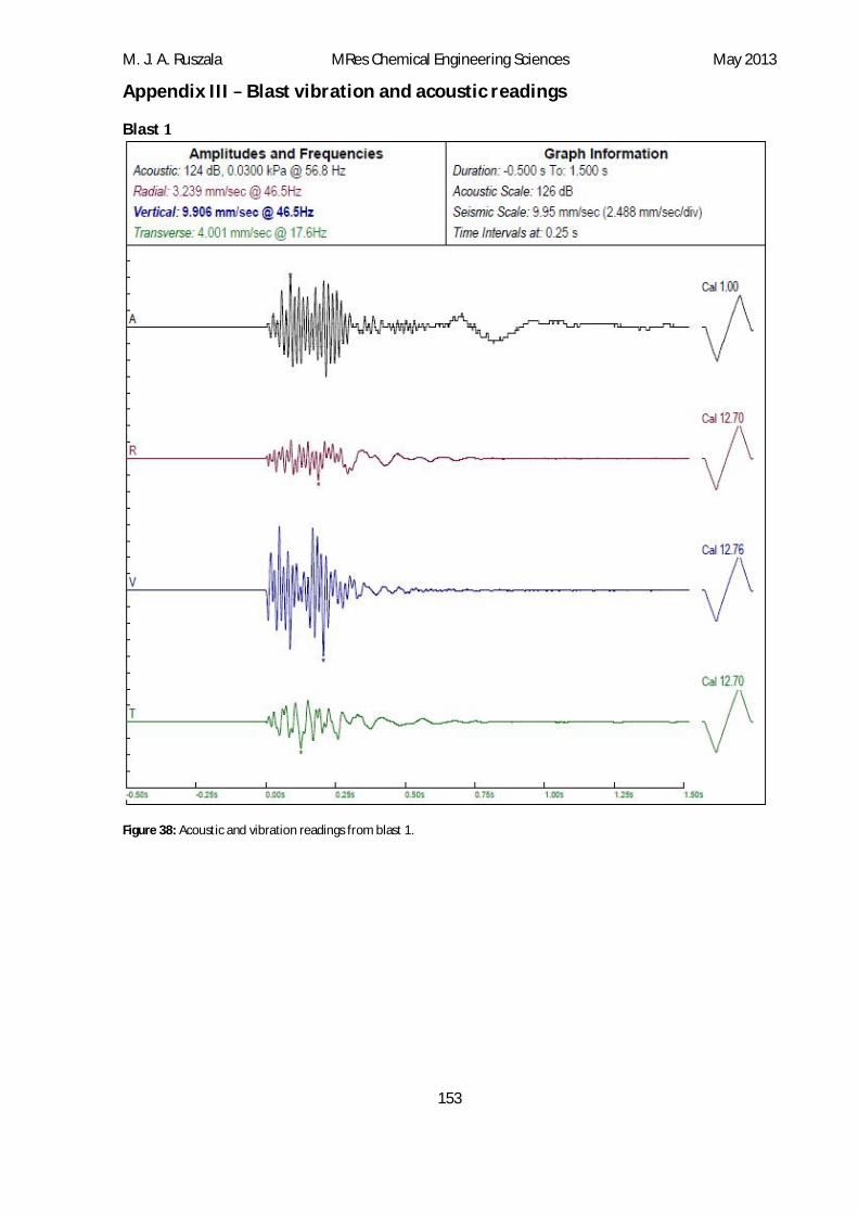
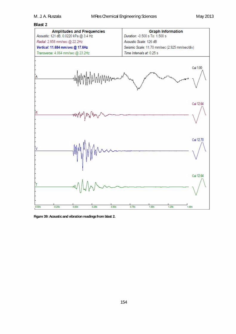


![[4317] – 328 - Savitribai Phule Pune · PDF file[4317] – 328 T.Y.B.Sc ... Explain the Ultra Structure of Cell wall ? Write its chemical composition and ... Name two countries with](https://static.documents.pub/doc/80x56/5aa54a557f8b9a517d8d051c/4317-328-savitribai-phule-pune-4317-328-tybsc-explain-the-ultra.jpg)

![[4317] – 201 - Savitribai Phule Pune University[4317] – 201 S.Y. B.Sc. (Semester – II) Examination, 2013 ... Marks : 40 1. Attempt any five of ... (Semester – II) Examination,](https://static.documents.pub/doc/80x56/5ad5720f7f8b9a075a8ce653/4317-201-savitribai-phule-pune-university4317-201-sy-bsc-semester.jpg)


