Brigham Young UniversityBYU ScholarsArchive

All Theses and Dissertations

1973-4

Finite Conductance Element Method ofConduction Heat TransferE. Clark LemmonBrigham Young University - Provo

Follow this and additional works at: https://scholarsarchive.byu.edu/etd

Part of the Mechanical Engineering Commons

This Dissertation is brought to you for free and open access by BYU ScholarsArchive. It has been accepted for inclusion in All Theses and Dissertationsby an authorized administrator of BYU ScholarsArchive. For more information, please contact scholarsarchive@byu.edu, ellen_amatangelo@byu.edu.

BYU ScholarsArchive CitationLemmon, E. Clark, "Finite Conductance Element Method of Conduction Heat Transfer" (1973). All Theses and Dissertations. 7146.https://scholarsarchive.byu.edu/etd/7146

£•£<7. 061-1-

Ls-n FINITE CDNDUCTANCE ELEMENT METHOD OF

CONDUCTION HEAT TRANSFER

A Dissertation

Presented to the

Department of Mechanical Engineering Science

Brigham Young University

In Partial Fulfillment

of the Requirements for the Degree

Doctor of Philosophy

by

E. Clark Lemmon

April 1973

This dissertation, by E. Clark Lemmon, is accepted

in its present form by the Department of Mechanical Engineer­

ing Science of Brigham Young University as satisfying the

dissertation requirement for the degree of Doctor of

Philosophy.

Date

ii

ACKNOWLEDGMENTS

The author wishes to express his appreciation to Dr. Richard

Ulrich, Dr. Howard Heaton, Dr. Henry Christiansen, and Dr. Richard

Hanks for their technical suggestions and encouragement relating to

this project and for their counsel in the preparation of this

dissertation. Dr. Heaton was especially instrumental in directing my

attention to the finite element and finite difference methods in

conduction heat transfer and directing my considerations of the

stability and oscillation criterion for the same. Together in 1969 we

presented a paper (14) at the ASME Winter Annual Conference which

contained some of the ideas presented in this dissertation. Dr.

Christiansen was very helpful in explaining the basic approach to the

finite element method in structures and in development of parts of the

computer program used. Dr. Ulrich was especially helpful in coordi­

nating the efforts of the committee and in directing my efforts in

pursuit of this degree. Special appreciation is also given to

Advanced Research Projects Agency (ARPA) for the full use of the time

share computer facility.

TABLE OF CONTENTS

INTRODUCTION...................................................... 1

THE FINITE CONDUCTANCE FACTOR AND ELEMENT....................... 3

BOOKKEEPING SYSTB1 AND SOLUTION TECHNIQUE......................... 31

NONCONDUCTION HEAT F L U X ............................................37

CHOICE OF CHARACTERISTIC TEMPERATURE............................... 45

CHARACTERISTICS OF FORMULATION AND SOLUTIONS....................... 57

COMPARISON OF DIFFERENT METHODS................................... 66

DISCUSSION OF RESULTS . . . ........................................ 76

CONCLUSIONS........................................................ 78

LIST OF REFERENCES.................................................. 79

APPENDIX.............................................................81

I

iv

5

7

1014

16

18

2022

23

25

27

29

41

46

46

51

51

63

69

LIST OF FIGURES

Rectangular Parallelopiped' One Dimensional FCE........

Rectangular Parallelopiped Two Dimensional FCE........

Rectangular Parallelopiped Three Dimensional FCE. . . .

Triangular Prism Two Dimensional FCE...................

Hexahedron Two Dimensional FCE Construction ..........

Two Dimensional FCE Validity...........................

Tetrahedral Three Dimensional FCE .....................

Three Dimensional FCE Validity.........................

Three Dimensional FCE Validity Extended ...............

Negative FCF's..........................................

Axisymmetric Two Dimensional FCE.......................

Triangular Ring Two Dimensional FCE ...................

Area and Volume Associated with Node...................

One Dimensional FCE Example ...........................

Superposition of Two One Dimensional FCE's............

Two Dimensional FCE Example ...........................

Superposition of Four Two Dimensional FCE’s ..........

Prefered Hexahedron FCE Construction...................

Construction of Thermal Resistance for Two Dimensional Systems ...................................

v

NOMENCLATURE

area

directly applied nonconduction surface flux which is not controlled by a temperature difference

heat capacity, capacitance matrix

pseudo accumulation flux

all internal sources and sinks except for D

all nonconduction heat fluxes

finite conductance element

finite conductance factor

all internally generated heat fluxes

convective or radiative conductance, convection matrix

separation variable

specified temperature vector

thermal conductivity, conductance matrix

length

temperature transformation matrix, separation variable

superposition transformation matrix

pseudo time, separation variable

conduction heat flux (energy/time)

surface convective heat flux controlled by a temperature difference

temperature, temperature matrix

unspecified temperature vector

volume

a,b,c,d,e lumping variables

i,m nodes, node counters

n number of dimensions, and counter on summations

P counter on time

w weighting factor

r,x,y,z space coordinates

A difference

time parameter

p density

0 K APpC V

y , v , x separation constants

6, n lumping variables

a positive constant

Superscripts

A matrix AA

As

X

vector A

special form of matrix A

XT transpose of matrix A

A 1A

Tc

inverse of matrix A

characteristic value of vector TArjicl correct or actual value of vector TA

Te the error in the vector T

Subscripts

A*A

Ai

expanded form of matrix A

i*k term of vector A

term of matrix A

convective driving temperature vector

INTRODUCTION

One of the basic goals in engineering is to formulate models

which will provide a means for analytically predicting observed

phenomenon. For some time, the partial differential equations

describing the steady state and transient conduction of heat within a

solid have been available. However, the straight forward use of these

equations is often restricted due to the surface geometry of the solid.

If the surface geometry is at all irregular, exact solutions will in

general not exist. In that case, a solution is sought by some

approximate numerical technique. The two techniques most often used

are the finite difference method and the finite element method. The

finite difference method is fairly simple to understand, but is

difficult to apply to a problem with irregular boundaries. On the

other hand, it is not a trivial matter to completely understand the

finite element method, although it can handle irregular boundaries with

greater ease than the finite difference method. To bridge the gap

between these two methods, a third method is developed in this work

which has the simplicity of the finite difference method, and can

handle irregular boundaries with the ease of the finite element method.

The method to be developed is the finite conductance element

method. With this method, the volume of interest if "filled" with

finite conductance elements (FCE) which may be thought of as conduct­

ance building blocks. For each FCE, several finite conductance factors

(FCF) are defined which may be regarded as a foim of Fourier's law of

1

heat conduction in discrete form. After the solid has been "filled"

with FCE's, each of which may have an external shape of a rectangular

parallelepiped, a tetrahedron, or a triangular prism, an accounting of

the conduction of thermal energy within the total volume may be made.

This accounting is done with a bookkeeping method that employs a matrix

shorthand technique. Using the bookkeeping method developed, the

"filling" of the volume of interest with FCE's is simply done by

superposition of matrices. The resulting matrix system represents a

set of simultaneous equations which may be solved in any convenient

manner to obtain the values of the parameters of interest.

The FCE method is here formulated only for isotropic materials.

In general, most practical problems are concerned with such materials.

However, a method is given whereby the FCE method may be extended so

that anisotropic materials may be used.

For additional clarification, two simple example problems have

been included as an appendix. It is recommended that reference be made

to them during the reading of this work.

THE FINITE CONDUCTANCE FACTOR AND ELEMENT

Introduction

The solid, in which the conduction of heat, is to be approxi­

mated, is "filled" with conduction building blocks which are named

finite conductance elements (FCE). These FCE's may have the shape of

a rectangular parallelopiped, a tetrahedron, or a triangular prism.

For each FCE, finite conductance factors (FCF) are defined which may

be regarded as a form of Fourier's law of heat conduction in discrete

form. These FCF's are developed in a consistent manner such that

there is no overlapping of material within the FCE.

The Finite Conductance Factor (FCF)

Fourier's law in discrete form for one dimensional conduction

of heat in a homogeneous isotropic material between nodes i and m using

a consistent set of units is

where Q. is the net conduction heat flux from i to m, K is the thermal\L-m ’conductivity, A is the cross sectional area associated with the con­

duction of heat from i to m, L is the distance from i to m, and AT.l-mis the temperature difference (TL-T ). The parameter (KA/L) is defined

as the finite conductance factor (FCF) between i and m. Equation (2.1)

may then be represented as

Q.\L-m (2.1)

Q. = FCF. m AT. . x i - m l - m l - m(2 . 2)

3

4FCF's will now be defined for several different FCE's. Each FCF will

be defined so that the conduction of heat within each FCE will be

accurately accounted for. This will be done by choosing the proper

area to be associated with the conduction of heat in each direction.

The finite conductance element (FCE)

The solid of interest is "filled" with many smaller imaginary

solids having the shapes of a rectangular parallelopiped, a triangular

prism, or a tetrahedron. For these conduction building blocks FCF's

are defined so that the one, two, or three dimensional conduction of

heat within the solid may be modeled. This conduction building block

is a finite conductance element (FCE). A consistent procedure is to be

followed in developing the FCF's for each FCE. This procedure is

simplified by the use of several figures and examples that will follow.

After the examples are given, the general procedure to be followed

will be stated.

One dimensional FCE

The finite conductance element (FCE) for a solid in which the

conduction of heat is completely one dimensional (say the x direction)

is a rectangular parallelopiped with a unit height (in the z direction)

and depth (in the y direction) and length L in the direction in which

heat is conducted (see Figure 2.1a). This FCE has two nodes, one at

each end of the FCE. One node is the y-z plane defining the left end

of the FCE and the other is the right end plane defining the right side

end of the FCE. Note that at each node, there can be no variation of

temperature, since temperature differences can occur only in the x

direction. This FCE is "cut" by a plane which is the perpendicular

Direction of Heat Conduction

Right End of FCE

Cutting Plane

Fig. 2.16

Fig. 2.1--Rectangular Parallelopiped One-Dimensional FCE

bisector of an imaginary vector (termed the leg vector) drawn from the

left end node to the right end node which lies in one of the edges of

the FCE (see Figure 2. lb). The intersection of the cutting plane with

the side planes defining the FCE define an area on the cutting plane

which is termed the cut area. The FCF for the FCE is defined as the

conductivity times the cut area divided by the length of the leg vector.

Two dimensional FCEFor a solid in which the conduction of heat is two dimensional

(say the x and z direction) one of the FCE's to be developed is also

a rectangular parallelepiped. This parallelopiped is of length Lx in

thex direction, Lz in the z direction and unit depth in the y direction

(see Figure 2.2a). This FCE has four nodes. Each node is an edge of

the FCE which lies completely in the y direction. Note again that

there cannot be a variation of temperature in any of the nodes. Four

leg vectors are now defined. Each leg vector is drawn from one node

to another and lies completely in one of the FCE edges. Note that a

leg vector between node 1 and node 4 cannot be defined as there is no

single edge between node 1 and node 4. Each leg vector is now bisected

by a cutting plane which is perpendicular to that leg vector (see

Figure 2.2b). Note that the four cutting planes share a common line

and that all of the nodes and the common line are parallel and lie

completely in the y direction. The cut area on each of the four

cutting planes is determined by the three lines of intersection formed

by the cutting plane with each of the three sides of the FCE and by

the common line. The FCE is now segmented into four pentahedrons as

illustrated in Figure 2.2c. Each pentahedron is uniquely defined as

illustrated by two nodes and by the cut area on the cutting plane of

Fig. 2 .2--Rectangular Parallelopiped Two-Dimensional FCE

8

the leg vector between the two nodes. The FCF for each pentahedron is

now defined as the conductivity times the cut area on the cutting

plane of that pentahedron divided by the length of the leg vector

between the two nodes on the pentahedron. This FCE then has four

FCF's, one for each of its segmented parts.

Three dimensional FCE

A rectangular parallelopiped may also be used as a FCE in a

solid where heat is conducted in all three directions (see Figure

2.3a). This FCE has eight nodes, one at each comer of the rectangular

parallelopiped. In this case, each node must be a point as the temper­

ature may vary in all three directions. Twelve leg vectors are now

defined. There is one leg vector in each edge of the FCE. As before,

each leg vector "connects" two nodes and lies completely within an

edge of the rectangular parallelopiped. Each leg vector is bisected

by a cutting plane which is perpendicular to that leg vector (see

Figure 2.3b). Note that the twelve cutting planes share a common

point. The cut area on each cutting plane is determined by four lines

in the cutting plane. Two lines are the lines of intersection of the

cutting plane with each side of the FCE in which the leg vector lies.

The other two lines are the lines of intersection of the cutting plane

for that leg vector and the cutting planes of the other leg vectors

which are not parallel to the leg vector being considered (see Figure

2.3b). These last two lines pass through the common point. The FCE

is now segmented into twelve hexahedrons as illustrated in Figure 2.3c.

Each hexahedron is uniquely defined as illustrated by two nodes which

are connected by a leg vector and by the cut area of the cutting plane

of that leg vector. The FCF for each hexahedron of the FCE is defined

Leg Vector

Fig. 2.3b

2.3--Rectangular Parallelopiped Three Dimensional FCE

10

Hexahedron

Fig. 2.3c

Fig. 2.3--Rectangular Parallelopiped Three Dimensional FCE

11as the conductivity times the cut area divided by the leg vector length.

This FCE then has twelve FCF's, one for each of its segmented parts.

Procedure used to develop FCE's

Three different kinds of FCE's have been developed. The

method used will now be given in general terms. The procedure outlined

will then be used to develop additional FCE's.

The general procedure to be used to develop FCE's for a

Cartesian coordinate system is as follows:

1. The shape chosen for a FCE is a polyhedron. For a system

where the conduction of heat is one dimensional, two of the face planes

on the polyhedron must be equivalent and parallel and be perpendicular

to the direction of heat flow. The term equivalent in this case means

that when the edges of these two planes are viewed looking in the

direction of heat flow that the edges completely coincide. All of the

other face planes must be parallel to the direction of heat flow. In

a system where the conduction of heat is two dimensional, two of the

face planes of the polyhedron must be equivalent and parallel and be

perpendicular to the direction in which heat flow cannot occur. In

this case, the term equivalent means that when the edges of these two

planes are viewed looking in the direction in which heat flow cannot

occur, that the edges all coincide. All other face planes must be

parallel to the direction in which heat flow cannot occur.

2. For each FCE, nodes are defined. A node is a region in

which a variation of temperature cannot exist. For a one (two, three)

dimensional FCE, the node will be a plane (line, point).

3. Each node is connected to all other nodes of the FCE where

there is at least one edge of the polyhedron between the two nodes. If

12there is more than one edge between two nodes, the edges must be

parallel. One imaginary leg vector is drawn between the two nodes and

lies in an edge of the polyhedron that connects the two nodes.

4. Each leg vector is bisected by a cutting plane that is

perpendicular to the leg vector.

5. All of the cutting planes must intersect in a common line

for systems in which the conduction of heat is two dimensional. In

systems where the conduction of heat is three dimensional, the cutting

planes must intersect in a common point. This common line (point) may

not always lie within the polyhedron.

6. Each cutting plane has a cut area on it that is bounded by

four lines. For a system in which the conduction of heat occurs in

only one direction, these four lines are determined by the intersection

of the cutting plane and the side planes defining the FCE. For a

system in which the conduction of heat is two dimensional, three of the

lines are determined by the intersection of the cutting plane and the

side planes of the FCE. The fourth line is the common line. In a

system where the conduction of heat is not limited to any direction,

two of the lines are determined by the intersection of the cutting

plane and the side planes defining the FCE. The other two lines are

determined by the lines of intersection of the cutting plane for that

leg vector and the cutting planes of the other leg vectors (which are

not parallel to the leg vector being considered). These two lines will

also intersect at the common point.

7. The polyhedron defining the FCE is then segmented into as

many smaller polyhedrons as there are leg vectors. For systems in

which the conduction of heat is one (two, three) dimensional the

13segmented polyhedron will be a rectangular parallelopiped (pentahedron,

hexahedron). Also note that each segmented polyhedron will always be

symmetric about the cutting plane.

8. The FCF for each of the smaller polyhedrons is defined as

the conductivity times the cut area on the cutting plane divided by

the leg vector length. If the smaller polyhedron associated with a

leg vector lies completely outside the larger polyhedron, its cut area

is considered to be negative.

Triangular prism two dimensional FCE

Often in problems where the conduction of heat is two dimen­

sional, the total solid of interest cannot be completely "filled" with

the rectangular parallelopiped FCE's previously developed. This

problem is usually caused by irregular boundaries. For these cases

another FCE shape is required. The simplest one possible is a

triangular prism as illustrated in Figure 2.4a where there can be no

conduction of heat in the y direction. Also, the angles and side

lengths of the triangular faces are arbitrary. The procedure for

developing FCE's previously given will now be used to complete the

development of this triangular prism FCE. This FCE has three nodes

which are the prism edges that lie completely in the y direction. The

imaginary leg vectors are now drawn between the nodes (see Figure 2.4a).

Each leg vector is bisected by a cutting plane that is perpendicular

to that leg vector as illustrated in Figure 2.4b. For an arbitrary

triangular prism the cutting planes will always intersect in a common

line as illustrated for this case. The cut area of each cutting plane

is now defined by the three lines formed by the intersection of the

cutting plane with the side planes of the prism and by the conmon line.

Fig. 2.4b

Fig. 2.4--Triangular Prism Two-Dimensional FCE

15

The prism is now segmented into three pentahedrons as illustrated in

Figure 2.4c. Note the similarity of these pentahedrons and the

pentahedrons obtained for the two dimensional rectangular parallelo-

piped FCE (Figure 2.2c). The FCF for each of these pentahedrons is the

conductivity times the cut area divided by the length of the leg vector.

If any other polyhedrons are to be developed to be used as a

FCE's for systems in which the conduction of heat is two dimensional,

the procedure previously outlined must be followed. Especially note

that the mutual intersections of the cutting planes must result in a

common line. For example, consider the hexahedron illustrated in

Figure 2.5a. For this polyhedron to be used as a FCE in a problem

where the conduction of heat is two dimensional (in the x and z

directions) two faces must lie completely parallel to the xz planes as

shown. The nodes would be the four edges parallel to the y axis as

illustrated. Following the procedure outlined for developing FCE's the

hexahedron is cut by the four cutting planes as illustrated in Figure

2.5b. However, for clarity, only the intersections of the four cutting

planes with the front face of the hexahedron are shown. Note that the

intersections of the four cutting planes do not result in a common

line. In this case six lines of intersection are obtained. Hence,

this hexahedron cannot be used as a FCE. However, this hexahedron is

not really necessary as any hexahedron of this general shape could be

built from two triangular prisms as illustrated in Figure 2.5c.

Equivalence of two dimensional FCE's

For solids in which the conduction of heat is two dimensional

two different FCE's have been introduced. The equivalence between

these two different FCE's can be established. For example, for the

16

Fig. 2.5c

Fig. 2.5--Hexahedron Two-Dimensional FCE Construction

17rectangular parallelopiped given in Figure 2.6a the overall conductance

in the x direction is the material conductivity times the cross

sectional area in the yz plane divided by the length of the parallelo­

piped in the x direction. One two dimensional rectangular parallelo­

piped FCE may be used to fill the rectangular parallelopiped illustrated

in Figure 2.6a (this was previously illustrated in Figure 2.2). The

overall conductance in the x direction is obtained by properly adding

the FCF's for the two pentahedrons which are segmented from the

rectangular parallelopiped which have conductance in the x direction.

These two pentahedron FCF's are in parallel, and the overall x

direction conductance is obtained by adding the FCF's for the two

pentahedrons in a parallel manner. That is, the overall x direction

conductance is equal to the FCF for the top pentahedron plus the FCF

for the bottom pentahedron. The result is that the overall x direction

conductance is correct.

The parallelopiped shown in Figure 2.6a can also be arbitrarily

segmented into triangular FCE's such as the arrangement illustrated in

Figure 2.4. The overall conductance in the x direction is then

obtained by properly adding the FCF's of the nine pentahedrons out of

the total twelve that have x direction conductance. This summation

requires adding of FCF's in both parallel and series. This, in

essence, has previously been done by Dusinberre (7). The resulting

overall x direction conductance of the rectangular parallelopiped is

correct. The same approach may be used to check the overall conductance

in the y direction. When this is done the correct results are again

obtained.

18

Fig. 2.6a

Fig. 2.6^-Two-Dimensional FCE Validity

19Tetrahedral three dimensional FCE

Often in problems where the conduction of heat is three

dimensional, the total solid of interest cannot be completely "filled"

with the rectangular parallelopiped FCE's previously developed. This

problem is usually caused by irregular boundaries also. For these

cases, another FCE shape is required. The simplest one possible is an

arbitrary tetrahedron as illustrated in Figure 2.7a. The nodes are

the four verticies of the tetrahedron and each edge of the tetrahedron

contains a leg vector. The intersection of each cutting plane with

the other cutting planes and face planes are illustrated in Figure 2.7b.

For an arbitrary tetrahedron, these cutting planes will always inter­

sect in a common point. The tetrahedron is segmented into six hexahe­

drons as is illustrated in Figure 2.7c. Each little hexahedron is

defined by the leg vector to which it is adjacent and the face area on '

the face plane adjacent to that by vector. For clarification, these

six hexahedrons are again shown in Figure 2.7d where the separation

distance is increased and the hidden lines are not included. Note the

similarity of these hexahedrons and the hexahedrons obtained for the

three dimensional rectangular parallelopiped FCE (Figure 2.3c). The

FCF for each of these hexahedrons is the conductivity times the cut

area on the cutting plane divided by the length of the leg vector.

If any other polyhedrons are to be developed to be used as a

FCE for systems in which the conduction of heat is three dimensional,

the procedure previously outlined must be followed. Especially note

that the mutual intersections of the cutting planes must result in a

common point as was the case with the rectangular parallelopiped and

the tetrahedron.

20

Fig. 2.7a

Fig. 2.7c Fig. 2.7d

Fig. 2.7--Tetrahedral Three-Dimensional FCE

Equivalence of three dimensional FCE's21

The equivalence between the two different FCE's previously

introduced to be used in a solid where the conduction of heat is three

dimensional can also be established. For example, for the rectangular

parallelopiped illustrated in Figure 2.8a the overall conductance in

the x direction is the material conductivity times the cross sectional

area in the yz plane divided by the length of the parallelopiped in

the x direction. This parallelopiped may be filled by one rectangular

parallelopiped FCE. The procedure used to obtain all the FCF's for

this FCE is to segment the parallelopiped into twelve hexahedrons as

was previously illustrated in Figure 2.3. The overall x direction

conductance for this FCE is then obtained by adding the FCF's of the

four hexahedrons that have x direction conductance in a parallel manner.

The result is that the correct x direction conductance is obtained.

The parallelopiped illustrated in Figure 2.8a may also be

segmented into five tetrahedral FCE's as illustrated in Figure 2.8b.

Each tetrahedral FCE is then segmented into six hexahedrons to obtain

all the FCF's for each FCE (this was previously illustrated in Figure

2.7). The result is that sixteen of the thirty hexahedrons have FCF's

with x direction conductance. All of these FCF's are in parallel. When

these FCF's are added in parallel the result is again that the overall

x direction conductance is correct. The same procedure may be used to

check the overall conductance in both the y .and z direction. Again,

the correct results will be obtained.

For additional emphasis, consider the rectangular parallelopiped

illustrated in Figure 2.9a. This solid may be segmented into four

hexahedrons as illustrated in Figure 2.9b. Each of these hexahedrons

22

Fig. 2.8b

Fig. 2.8--Three-Dimensional FCE Validity

23

Fig. 2.9--Three-Dimensional FCE Validity Extended

24

may now be segmented into five tetrahedral FCE's. As before, each

tetrahedron is segmented into six hexahedrons to obtain the six FCF's

for each tetrahedral FCE. The result is that sixty-four of the one

hundred twenty little hexahedrons have y direction conductance. These

sixty-four FCF's are in parallel. When these sixty-four FCF's are

added together in parallel the correct result is obtained for the

overall y direction conductance. This again indicates that the formu- .

lation of the tetrahedral FCE's is correct. In both the x and z

direction there are more than sixty-four hexahedrons that have either

x or z direction conductance. These FCF's are in a combination series

and parallel arrangement. When they are properly summed, the overall

conductance in each direction will also be correct.

Negative FCF's

For the triangular prism FCE (or tetrahedral FCE) the common

line (point) may not lie within the prism (tetrahedron). For example,

consider the triangular prism illustrated in Figure 2.10a. The cutting

planes are illustrated in Figure 2.10b. Note that the common line does

not lie within the triangular prism. This does not cause any special

problems in developing FCF's for a FCE. This is illustrated in Figure

2.10c where the resulting three pentahedrons are shown. Again, the

FCF for each pentahedron is the conductivity times the cut area on the

cutting plane divided by the length of the leg vector. However, if the

cut area on the cutting plane lies completely outside the original

triangular prism, the cut area is assigned to be negative. For the

triangular prism illustrated in Figure 2.10a, the FCF for the bottom

pentahedron in Figure 2.10c is negative. Negative FCF's are not

bothersome as a FCF in itself is not complete, it is only one part of a

25

Assigned to be Negative

Fig. 2.10c

Fig. 2.10--Negative FCE's

26

FCE. Although it is considerably more difficult to sketch the

analogous situation for a tetrahedral FCE, the same results occur.

That is, the common point for a tetrahedral FCE may also lie outside

the tetrahedron. This results in at least one of the FCF's for the

FCE to be negative. As before, if a cut area lies completely outside

of the tetrahedron, the FCF for that hexahedron is assigned to be

negative.

Axisymmetric two dimensional FCE's

For solids in which the conduction of heat in an axisymmetric

coordinate system is two dimensional, the FCE's previously defined (for

solids in a Cartesian coordinate system in which the conduction of heat

was two dimensional) may be extended to define two axisymmetric FCE's.

This is done by considering the basic element to be a ring instead of a

polyhedron. The first ring FCE is illustrated in Figure 2.11a. This

rectangular cross section ring is symmetric about the x axis and the

cross section sides are either parallel to the x or r axis as illustrat­

ed. The four nodes are the edges of the ring. The procedure to be

followed to develop FCF's for this FCE is analogous to that used to

develop FCF's for the two dimensional rectangular parallelopiped FCE

except that instead of using cutting planes, a segment of a line of

revolution is used. This results in the segmentation of the rectangular

cross section ring into four triangular rings. This is illustrated by

the dotted lines in Figure 2.11b. The FCF for each triangular cross

section ring is the material conductivity times the area on the line

segment of revolution divided by the distance between the nodes.

Often, even though, the conduction of heat in an axisymmetric

solid is two dimensional, the solid cannot be completely filled with

27

x

Fig. 2.11a

x< i

One of Four LineSegments ofl^ Revolution

One of FourTriangular Segmented Rings

- ► rFig. 2.11b

Fig. 2.ll--Axisymmetric Two-Dimensional FCE

28the rectangular cross section ring FCE just developed. To handle this

case the other axisymmetric FCE to be developed has an arbitrary-

triangular cross section as illustrated in Figure 2.12a. The same

procedure followed to develop the other axisymmetric FCE is again

followed. This results in the triangular ring being segmented into

three triangular rings as illustrated in Figure 2.12b. As before, the

FCF for each segment is the conductivity times the area on the line

segment of revolution divided by the distance between nodes. In some

cases, the common line ring, which is created by the common intersec­

tions of the three line segments of rotation, may lie outside the

triangular cross section ring. In this case, as before, the area on

the line segment of revolution that lies completely out of the triangu­

lar cross section ring is assigned to be negative which results in one

of the three segmented rings to have a negative FCF. Also, the

analogous procedure used before to show that the triangular prism FCE

was as valid as the rectangular parallelopiped FCE may be used to show

that the triangular ring FCE is as valid as the rectangular ring FCE.

Summary

The procedure to be followed in using the finite conductance

element method to approximate the conduction of heat within solids is

as follows:

1. The solid in which the conduction of heat occurs is "filled"

in an orderly manner with basic conduction building blocks which are

called finite conductance elements.

2. Finite conductance factors are developed for each finite

conductance element. These finite conductance factors may be regarded

as Fourier's law of heat conduction in discrete form.

29

x

Fig. 2.12--Triangular Ring Two-Dimensional FCE

303. A numerical accounting procedure is then employed to

account for the interaction of the different finite conductance

elements.

Within this chapter, the second step has been discussed. The

next chapter will develop the orderly manner to be used to fill the

solid with FCE's, and the numerical accounting procedure to be used to

monitor the interactions between the FCE's.

BOOKKEEPING SYSTEM AND SOLUTION TECHNIQUE

Introduction

The solid in which the conduction of heat is to be monitored is

numerically "filled" with finite conductance elements (FCE's). For

each FCE, finite conductance factors (FCF's) have been defined. These

FCF's may be regarded as a discrete form of Fourier's law of heat

conduction. Using these FCF's, an accounting of the heat flux at each

node of each FCE is made. The Bookkeeping system to be used employs

matrix shorthand techniques and is developed in this chapter.

Assembly of the FCE

At each node of a FCE an accounting needs to be made of the

nodal temperature, the net nonconduction heat flux to the node, and

the net heat conducted to the node from the other nodes in the FCE.

The net flux entering and leaving node 1 is

F1 (3.1)

where F^ is the net nonconduction heat flux into node 1, is the

net conduction heat flux from node 1 to node i, and n is the number of

nodes in the FCE. Similar expressions exist for all other nodes of the

FCE. The FCF between node 1 and node i was defined as

Qi-i == FCF.1-i ATl-i*

31

(3.2)

Hence, Equation (3.1) may be represented as32

n£i-2 (FCFl-i ATl-i )' (3.3)

Now, a FCE has from two to eight nodes, depending on which FCE it is.

For any FCE, each node can be represented by an equation like Equation

(3.3). These n equations may be put in matrix form. For example, for

n equal to four the matrix form of the equations is

2FCFl-i "FCF1_2

-FCF2-1-FCF

-FCF

ZFCF2-i

3-1 ■FCF3-2

4-1 -FCF4-2

-FCF1_3 -FCFi_4

-FCF2-3 ~FCF2-4

£FCF3-i "FCF3-4

-FCF4_3 SFCF4. i

(3.4)

wheren

2 FCFk.i ■ FCEi=l k-i'

The square matrix will always be symmetric about the diagonal.

If, of course, there is not a direct conduction path between two nodes,

the corresponding FCF will be zero. The above matrix equation will be

represented as

Fa - Is Ta (3.5)

/ v / \

where Fa is the complete nonconduction flux vector of FCE a, Ta is the

complete temperature vector for FCE a, and K9 is the matrix constructed

Vf2

F3

F4

VT 2

T3

T4

33as in Equation (2.4) from all the FCF's for FCE a. K is called the

conductance matrix.

Filling of solid with FCE's

For a system containing several FCE's the accounting system is

expanded by matrix superposition to account for all of them. In filling

the volume of interest with FCE's, a node is common to all adjacent

FCE's. For each FCE there exists a matrix equation of the form

F1 = K1 T1 . (3.6)

For the whole system a similar matrix equation is obtained as

F = K T (3.7)

where

F = I F1 , K = I K1A * A *

T is the complete temperature vector for the system. The determination

of the starred matrices is obtained by considering how the T vectorA

may be obtained from the T vector. This is done by a superposition

transformation matrix IT as

A • • A

T1 = N1 T . (3.8)

It immediately follows then that

~i —iT Ai F1 = N1 F *

34and

(3.10)

• rp •where N11 indicates the matrix transform of N1 .

Solution technique

For the set of FCE's forming the complete system, accounting

procedures have indicated that

For each specific problem the K matrix will be completely known and at

each node either F^ or will be given in some form. That is, if

is constrained to a particular value, F^ cannot be constrained, and

vice versa. The knowledge of which nodes have constrained temperatures

may be described in matrix form as

J is the set of constrained temperatures, U the remaining unspecified

temperatures, and U is the transformation matrix required for the twoA A

sides of the equation to be equal. The vector J is the same size as T

with all the constrained values properly placed and with any value

(such as zero) in positions corresponding to nonconstrained temperature/A /A

nodes. The vector U may be considerably smaller (less rows) than T as

it contains only the nonspecified temperature nodes. With Equation

(3.12), Equation (3.11) may be represented as

F = IT T . (3.11)

T = H U + J . (3.12)

F = K (FT U + J) . (3.13)

35_T

Multiplying both sides of Equation (3.13) by M (to obtain a squareA

matrix that can be inverted), rearranging and solving for U gives that

U = ^ K M ) " 1 # ( F - K J ) . (3.14)

Now all of the terms on the left of Equation (3.14) have been specifiedA

except for F which is only partially known. However, premultiplicationA m A

of F by M 1 multiplies every unspecified term in F by a zero so thatA rp A

even though F is not completely specified, ffF is. Also, premultipli-_ t _

cation of K by M clears out all rows in K associated with points havingTspecified temperatures and post multiplication of 5T K by M" clears out

Tall columns of associated with specified temperature nodes. Hence,/s

once the operation indicated by Equation (3.14) has been completed, TA

can be determined from Equation (3.12) and F from Equation (3.11). The

solutions to any of the matrix equations may be obtained in anyT1

convenient manner. The only constraint is that M" W cannot be

singular. However, since the diagonal term on any row of K is always

equal to the negative sum of the off-diagonal terms on that row, and

the post multiplication of K by 5T simply eliminates some of the termsT _

on that row other than the diagonal term, the matrix 5T W cannot ever

be singular.

The first example problem given in the Appendix illustrates the

application of the finite conductance element method which has been

given up to this point.

Summary

In this section the method of accounting of nodal temperatures.

and fluxes within a FCE have been described. This method was then

36extended to several FCE's by a matrix superposition scheme. A linear

matrix transformation was then introduced to handle the problem of

nodes that were constrained in temperature to yield a set of simultan­

eous equations to be solved to obtain the unknown quantities. In the

next section, the nonconduction flux term will be clarified and

expanded so that the FCE method may be used to also approximate

transient heat conduction problems.

NONCONDUCTION HEAT FLUX

Introduction

Each finite conductance element occupies a certain volume of

material. Thermal energy is transferred into and out of the nodes of

the FCE. Each node has a portion of the total volume of the FCE

associated with it. The net conduction heat flux that leaves each

node is equal to the net nonconduction heat flux that enters each node.

In general, this nonconduction heat flux will be a function of the

volume or area associated with each node. Within this chapter this

nonconduction heat flux term will be expanded.

Volume associated with a node

The procedure followed to obtain FCF's for each FCE required

that each FCE be segmented into as many polyhedrons as there were leg

vectors. These polyhedrons were always symmetric about the cut area on

the cutting plane which was a perpendicular bisector of each leg vector.

The total volume of each polyhedron is then also cut in half by the

cutting plane. Each half volume is then associated with the node to

which it is adjacent. The total volume then associated with each node

is the sum of all the half volumes of all the segmented polyhedrons

adjacent to that node. In this way, the total volume of the FCE is

accounted for. Note that this requires that if a cut area is assigned

to be negative, that the volume of that segmented polyhedron is also

assigned to be negative.

37

38

Thermal energy conservation

The conservation of thermal energy in the volume associated

with each node requires that the rate at which thermal energy is stored

is equal to the net rate of thermal energy inflow. This thermal energy

inflow consists of conduction and nonconduction terms. If, however,

the accumulation tern is considered as a nonconduction term, the

conservation of thermal energy requires that the net outflow of thermal

energy by conduction from a node is equal to the net inflow of noncon­

duction thermal energy.

The nonconduction heat flux to the volume associated with node

1 may be a summation of many different types of fluxes as

F. = 1 R. + B. + G.i l l (4.1)

where is all convective fluxes to node i applied on surfaces

associated with node i that are controlled by some kind of temperature

difference. This includes all boundary constraints generally termed

convection or radiation. is all directly applied surface fluxes to

the surface area associated with node i that are not controlled by a

temperature difference, and is all generation heat sources that

occur within the volume associated with node i including accumulation.

The convective flux R^ may be expressed as

R. = H. A. AT?l i l l (4.2)

where If is the convective heat transfer coefficient per unit area,

is the area over which convection is applied, and AT^ is the character-

39

istic temperature difference of the area associated with node i over

which the convection is applied - this is the temperature difference

driving the convection. This will handle both general convective and

radiative fluxes if IE is allowed to be a function of T? or AT?. The

directly applied flux in general may be expressed as

where T? is the characteristic temperature of the area associated with

node i on which the flux is applied. The heat generation term may

be expressed as

(4.4)

Qwhere T^ is the characteristic temperature of the volume associated

with node i, and is the volume associated with node i. The heat

generating source term can be split into at least two categories as

G ± = \ * Di (4.5)

where is the net accumulation of thermal energy in the volume

associated with node i, and is all other internal sources and sinks

in the volume associated with node i.

Thermal energy conservation in the volume associated with each

node requires that the rate at which thermal energy is stored is an

additional sink term that must be included. The net accumulation of

thermal energy in the volume associated with a node expressed in

discrete form is

40

D.1p. C. V. Ki 1 1— AV —

cTi , p+1 (4.6)

where is the density of material associated with node i, Ch is the

specific heat capacity of material associated with node i, is the

volume associated with node i, and is the characteristic temperature

of node i. The term AP is equal to (Pp+^ - P ) where P is time and the

subscripts on P are counters on time. The term R may then be repre­

sented as

F.l H. A. AT- + B. + E..i l l l lp- C. V- /Mi 1 l T c

AP \ i,p+l (4.7)

Characteristic temperature

Each component of the flux is dependent on either some area

or volume associated with the node, and some characteristic temperature

of that area or volume. The determination of the characteristic

temperature is not trivial. Consider the tetrahedral FCE shown in

Figure 4.1 which has been segmented into the volumes associated with

each node. If convection is applied on the face nearest the reader the

area to be used for convection at node 1 is obvious - but, what is the

characteristic temperature to be used? One possibility would be to

use the average temperature that exist on the area used for convection

at that node. The use of Fourier’s discrete conduction equation carries

the assumption that the temperature variation between any two nodes is

linear. In that case the functional relationship is

Fig. 4.1--Area and Volume Associated with Node

42

t J = cr1 , t 2 , t 3) (4.8)

with the strongest dependence on T^. Also, it a heat flux is dependent

on the characteristic temperature of the volume associated with node 1,

then the functional relationship becomes

- Tj (Tp T2, T3, T4) (4.9)

with the strongest dependence on T^.

Nodal temperature assumption

If the approximation is now made that

(4.10)

then Equation (4.7) may be expressed as

F.l Hi Ai (T.I00 + B. + E.l lp. C. V.Ki l l

AV)• (4.11)

Equation (4.11) though, is not yet completely specified. It is

apparent that each term must also be associated with some time p. In

Equation (4.11) some terms are evaluated at (p + 1) and some at (p).

Hence, all other terms may be specified at any time in between (p) and

(p + 1). This is so done by Equation (4.12).

F.i = <f> Bi + E..1P+1(4.12)

p.C.V.Hi l lw

T.i»P )•

43

The term <J> is constrained to be 0 > <j> >_ 1. For each FCE, the F vector

will now be given as

A I / A A \ A A A

F = <J> H (T^ - T ) + B + E - C T p+1 (4.13)

+ (I-*)/\ A\ A A

H ( T ^ - l j + B + E + U T

Both the H matrix and the C matrix are diagonal matrices with H.liH. A. and C.. = p. C. V./AP. i i n Ki i i

The complete set of equations for the group of FCE’s is

F = K T . (4.14)

A

If the term KT in Equation (4.14) is evaluated some where between p

and (p + 1), then

F = 4> (Tf)p+1 + (1-4)) (ri)p . (4.15)

If Equation (4.15) and Equation (4.13) are now combined the accounting

matrix representation obrained is

= r 5 Ts (4.16)

where

F= = e )' + [c t ]p+1

FT T + B + E - H T - K TP ’+ (1-40

4> (H + K) + C 9K5P+1

44

The superscript s flags the special forms indicated above. Now atAC

each time level, the vector T may be described as

TsP+1

(4.17)

A

The solution of the system for U is then

(4.18)

Of course, for this operation to be possible, the matrix FT must be

nonsingular.

Summary

The nonconduction heat flux term has been expanded to include

convective and radiative fluxes, surface fluxes, internal source or

sink fluxes, and an accumulation sink term. The characteristic

temperature of a surface or a volume was introduced. This character­

istic temperature was some kind of average temperature of the given

area or volume. The expansion of the accounting system necessary to

handle these additional flux terms has been developed. However, the

choice of the characteristic temperature as the nodal temperature has

not been justified. This is attempted in the next section.

CHOICE OF CHARACTERISTIC TEMPERATURE

Introduction

Within this section the choice of the characteristic tempera­

ture as the nodal value is justified. This is done by considering the

implications of the choice on the stability and oscillation criterion

of the system, and the effect on the accuracy of the results.

Stability and oscillation criterion

Some of the implications of choosing the characteristic

temperature to be other than the nodal temperature is illustrated by

the examination of the completely interior FCE shown in Figure 5.1 and

by considering the choice of the characteristic temperature for each

node. The accumulation term for node i for constant properties with

1A equal to the volume associated with node i is

Since the temperature variation through the FCE is linear, and since

the left one-half portion of the volume is associated with node i, the

characteristic temperature in Equation (5.1) could be chosen as

T- = w T. + (1-w) Ti+1 (5.2)

| < w < 1.45

where

46

Node i

Fig. 5.1--One-Dimensional FCE Example

Fig. 5.2--Superposition of Two-One-Dimensional FCE's

With the weighting factor w equal to 3/4, the characteristic tempera­

ture is the average temperature of the volume associated with node i,

and w equal to 1 sets the characteristic temperature equal to the

nodal temperature. For such a general case. Equation (5.1) may be

represented as

When the characteristic temperature is chosen as the nodal temperature

the matrix C for this element is

where V is the volume of the FCE. However, choosing the characteristic

temperature in the general way described by Equation (5.2) the C

matrix is

(5.3)

Pi C± V 1 0(5.4)

2AP [0 1 J

Pi Ch V w 1-w(5.5)

2AP 1-w w .

For the two adjacent FCE's illustrated in Figure 5.2 the

accounting matrix equation is

c =

r

Di " -

FS = Is TS .

r =

C5.6)

48For these two FCE's, B, E, and H are all null. Equation (5.6) then

reduces to the following:

[c t ] - (1-40 (k t ] = [(<}> K + C ) T ] . (5.7)p y p+1

With constant properties and equal volumes, the equation for node i

reduces to the following:

[a I,., - b T. * a T1+1]p+i - [c (5.8)

where

a = ~ 9<j>, b = w + 29(j>, c = + 0 (l-<j>),

d = w - 20 (1'H and 0 - ^ .

The L term comes from the volume of the FCE which is equal to the

length L times a unit depth times a unit height. The terms a, b, c,

d, and 0 are all dimensionless.

If T^ is assumed to be equal to the product of a variable I

dependent only on space position, and a variable P dependent only on

time level, then

Ji (5.9)

If Equation (5.9) is substituted into Equation (5.8), Equation (5.8)

after rearrangement may be represented as

49

U (5.10)

where y is a constant since P and I are independent. Equation (5.10)

may then be separated as follows:

(5.11)

h - i “ V h + i 0

where

d - cX , _ d - byp ” b - aX * c - ay

The exact solution of the difference Equation (5.11) for I requires

that I XI< 2 and the exact solution for P is

Pp = yp . (5.12)

Examination of Equation (5.12) indicates that for the numerical solu­

tion to be stable, that IyI< 1 and in addition, if no oscillations are

to be permitted, y must be positive. From the definition of the.

terms a, b, c, and d in equation (5.8) and the definition of y in

Equation (5.11) it follows that

c 1 . ^ . d l . u Ii+1a I — litl

50

2 (l + £j[v<|> + (1-40(5.13)

if oscillations are to be avoided. The term 6 is directly proportional

to the largest time step that can be taken and yet maintain stability

and permit no oscillations. It is advantageous to be able to choose

0 as large as possible when obtaining the approximate solution to a

problem. Equation (5.13) then indicates that for a set value of p and

<f>, that 0 is directly proportional to w. Hence, the larger the value

of w, the larger the allowable time step. From this standpoint the

obvious choice is to choose w as one, which indicates that the charac­

teristic temperature is the nodal temperature.

Two dimensional FCE stability

The same conclusions apply to other types of FCE's . For

example, for a two dimensional FCE shown in Figure 5.3, the choice of

the characteristic temperature for T? m is

(5.14)

where

I F - w - 1 •

51

i-l,m+l i,m+l

111

a .,m i

Fig. 5.3--Two-Dimensional FCE Example

i-l,m+l i,m+l i+l,m+l

i-lpn L,m i+l,m

i+l,m-l

Fig. 5.4--Superposition of Four-Two-Dimensional FCE’s

The C matrix for the FCE with constant properties and with V the

volume of the element is

52

7T _ p C V 4 A P

w 7 (1-w) T (1-W) 7 (1-w)

J (1-w) w \ (1-w) 7 (1-w)

(5.15)

7 (1-w) 7 (1-w) w 7 (1-w)

7 (1-w) 7 (1-w) J (1-w) wI

For the four adjacent interior FCE's illustrated in Figure 5.4 the

accounting matrix equation is Equation (5.6) which also reduces to

Equation (5.7). With constant properties and equal volumes and side

lengths. Equation (5.7) may be represented as

A A

[ a d a d e d a d a ] Tp+^ = [a b a b c b a b a] (5.16)

where

T T T T Ti-l,m-l i,m-l i+l,m-l i-l,m i,m

^i+l,m ^i-l,m+l Ti,m+1 ^i+1,m+ll’

a - , b - (1-w) + 0 (l-<}>), d - (1-w) - 4>9»

= I ‘ 4 0 Cl-4>) » e = 7 + 4 9 * , e = ^ •c

Again, if a product solution form of.53

T.i,m,p I. M P i m p (5.17)

is chosen. Equation (5.16) may be separated as follows:

(5.18)

Mm+1 + X M + M , = 0m m-1

I. , + v I. + I. , = 0 l+l i l-l

where

.. _ (c-ey) - A (b-dy) _ (c-bv) + A (av-b) (b-dy) - X (a-ay) * ^ (e-dv) + A (av-d)

The exact solution of the difference equation for P is the same as

before, that is

P = yF . P

(5.19)

Again, solving the equation for y and obtaining the restricting value of

0 results in the relationship

0 < ( i - y )/. ̂ 6v + 6A - vAi / 6v + 6A - vA \

w (4 * 7 — H 7 ) I ■8 (4 + v + A) [y <f> + (!-<)>)]

(5.20)

54

From Equation (5.20) it is again obvious that from a standpoint of

stability and oscillations that the best choice is to choose the charac­

teristic temperature as the nodal temperature.

Accuracy

Another consideration that must be made in selecting the charac­

teristic temperature is that of accuracy. The truncation error of

Equation (5.8) was obtained by Lemmon and Heaton (14) by the usual

Taylor series method to be of the order of the element length squared

unless

e (i ~ $) + ( V 9 ■ it - ° (5-21̂

in which case the error will be of the order of the element length to

the fourth power. Note that if <j> / ^ and if the properties are not

constant, 0 will not be constant either, requiring a variable time step

to maintain minimum truncation error. Hence, the choice of a character­

istic temperature other than the nodal value does not in itself insure

a decrease of the truncation error unless other conditions are also met.

This same trend is also true for the other FCE types.

The equations given for the maximum values of 0 and for estimat­

ing the truncation error are given only to indicate the implications of

the choice of the characteristic temperature. Similar requirements

exist for FCE's on boundaries which in general are more complex and more

restrictive. However, the trends will remain the same.

55Characteristic temperature choice

Hence, in favor of choosing the characteristic temperature

different than the nodal temperature is the possibility of a decrease in

the truncation error. On the other hand, the points in favor of

choosing the characteristic temperature equal to the nodal temperature

are the following:

1. The allowable time step will be the maximum.

2. Construction of the different non-conduction flux matricies

will be simplified and quicker and less computer storage will be required.

3. Computation, per time step, will be less since less terns

are carried.

4. The time step may be constant even if the properties are not.

In general, it is recommended that the characteristic temperature be

chosen as the nodal value. The choice of the value of <j> is also

simplified by the equations of this section. Examination of the general

accounting matrix equation indicates that chosing <J> = 0 gives equations

that are explicit in time. Equations (5.13) and (5.20) indicate that

the larger cf>, the greater the allowable time step which suggest a point

in favor of chosing <j> = 1. However, Equation (5.21) indicates that if

* 4 -26 , the truncation error will be of the order of element

length to the fourth power. In practice, a value of <J> = j has been

found to be satisfactory.

The second example problem given in the Appendix illustrates the

application of the finite conductance element method which has been

given up to this point.

Summary

56

In this section it has been illustrated that the choice of a

characteristic temperature other than the nodal temperature in general

results in having to choose a smaller time step to avoid numerical

instabilities or oscillations. It has also been illustrated that the

choice of the characteristic temperature other than the nodal temperature

does not in itself insure an improvement in accuracy. Several other

reasons were also given to support the conclusion that in general, the

choice of characteristic temperature as nodal temperature is best.

Up to this point, a complete formulation of FCE's has been given.

However, no assurance has been given that the results obtained from such

a system will be unique, consistent, stable, and converge to the true

solution. These items are discussed in the next section.

CHARACTERISTICS OF FORMULATION AND SOLUTIONS

Introduction

The FCE method that has been formulated may be used to obtain

approximate solutions to conduction heat transfer problems if several

important requirements are satisfied. The major requirement is that the

solution obtained with the FCE method will truly model the conduction of

heat in the volume of interest. The characteristics of the formulation

of the FCE method, and the solutions obtained with the method, that

relate to the capability of the, method to adequately model the conduction

heat transfer problem are as follows:

1. Are the solutions unique?

2. Is the formulation well posed?

3. Is the formulation consistent?

4. Is the solution technique stable?

5. Will the solution converge to the true solution?

Unique solutions

The form of the set of equations describing the steady state

problem is

K T = F . (6.1)

A

For this form, a unique solution for T does not exist as by definition,

K is always singular. Recall that K is symmetric and that on any row

(or column) the negative of the diagonal term is equal to the sum of the

57

58

off-diagonal terms on that row (or column). This always forces the

matrix to be singular. To obtain a unique solution, it is necessary to

constrain at least one node. Equation (6.1) then becomes

( # K R ) U = # (F-KJ) C6-2:)

___which always has a unique solution since the matrix M K M is always

positive definite.

The expanded transient form of the equations are

Xs TS = FS (6.3) '

where

' f = ^ ( H + i O + c .

A

Again, for a unique solution for T s to exist the matrix K5 must not be

singular. If C is constrained to be positive-definite and each diagonal

term in the H matrix, which is a diagonal matrix, is constrained to be

nonnegative, then it follows that K5 is also positive-definite and hence

not singular.

Well posed and consistent formulation

For the formulation to be well posed, the numerical model must

not violate the basic physics in discrete form controlling the problem.

This formulation meets this requirement since Fourier's law in discrete

form has been used in a consistent matter, heat has been conserved within

discrete blocks of isotropic homogeneous material to form the overall

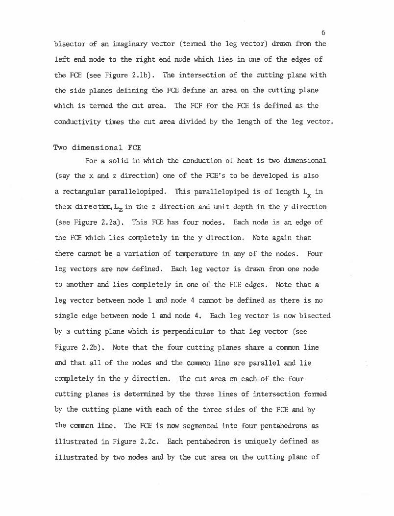
system. In addition, since the triangular prism FCE can be shown to be

as valid as the rectangular parallelopiped FCE and since the tetrahedral

59

FCE is also as valid as the rectangular parallelopiped FCE the resulting

system is really equivalent to the standard finite difference method

which is accepted as being well posed. The same argument is used to

suggest that the system of equations used are consistent, that is, as

the size of the discrete FCE goes to zero, and as the discrete time goes

to zero, the resulting equation reduces to the correct differential

equation.

Stability of solution form

The question of stability only applies to the transient problem

and refers to the accumulation of error due to computational round off.

The overall equation describing the system is

Fs = X s TS (6.4)

where

FS = n + (<j>-i) ( M ) Tp + C Tp ,

K5 = <P (K+H) + cr, fs = Tp+r

* As The vector n is all the other terms in F not listed. Equation (6.4)

may then be given as

(<t> S* + C) Tp+1 - n t [(4>-D S"+ C) Tp . (6.5)

/V A

If at some time p, an error is introduced into the vector T, T may

be described as

T = Ta + Te (6.6)

60where the superscript a refers to the actual or correct value and e

refers to the error. Equation (6.5) may then be represented as

[<}><$ + cj Ta + T6 p+l p+l n + [«-!) « (6.7)

Substituting in the correct value of n into Equation (6.7) gives after

rearrangement the recursion equation for the error in temperature as

Te , = S Tep+l p (6.8)

where

S = [<j> T + C]"1 [(<(>-1) I + ~C] .

Letting

a = S. . max ij (6.9)

the error at (P+l) is at most

P+1mV= a T (6.10)

since

“ t p i S T p (6.11)

61From the form of the recursion formula. Equation (6.10) is equivalent to

P+1aP T* (6.12)

Equation (6.8) is then equivalent to

[<f>6 + C] a T® = [(<J>-1) 7 + C] T® (6.13)

which after rearrangement becomes

1-a

. <P ( a - 1 ) + 1Tr = 0. (6.14)

If 6 is positive-semidefinite, which has been assured by the formulation,

and C is positive-definite (see for example, Wylie (19), chapter 11) then

1-q<j> (a - 1) + 1' > 0 (6.15)

or

a | < 1 . (6.16)

Equation (6.9) required that a be a positive constant and Equation (6.12)

then indicates that any introduced errors will not grow with time, which

indicates the system will be stable as long as Equation (6.14) is

satisfied. In general. Equation (6.14) cannot be satisfied unless C is

bounded which indicates that AP is also bounded. This is easily seen by

letting <|> equal zero. Equation (6.14) is then represented as

62

[6 - (l-o) C ] T® = 0 (6.17)

where the term (1-a) can be at most one and the interval from zero to

one cannot be guaranteed to be large enough to contain at the eigen­

values for a particular <T and C matrix.

Overall restrictions and convergence

The complete set of restrictions then required to guarantee that

the solutions will be unique and that instabilities may be avoided are

the following:

1. C is positive definite (with the characteristic temperature,

equal to the nodal temperature, C is a diagonal matrix. A diagonal

matrix is positive definite if every diagonal term is greater than zero)

2. AP in general is bounded (this restriction is relaxed as

<p t 1.) It is not necessary to require that S’ is positive-semidefinite

or positive definite as 6 is the sum of K and H. That is, K is always

singular and by adding H to K, the result, 6", is always positive-

definite unless H is null, in which case it is positive-semidefinite.

The first four questions posed have all been answered to the

affirmative (with certain restrictions). It then follows from Lax's

equivalence theorem that the answer to the fifth question is also

affirmative, at least to the order of maximum leg length squared.

The restriction of nonnegative, non-null values of is

generally not bothersome. Even though for a particular node of a FCE,

the V- may be negative or zero, by the time all of the FCE's having the

same node have been superimposed the resulting CL ̂ is generally not zero

or negative. This is especially true if the FCE is chosen in a preferred

manner. For example, the volume illustrated in Figure 6.1a is to be

63

Fig. 6.1--Preferred Hexahedron FCE Construction

64

divided up into triangular prism FCE's. This may be done in either of

two ways as illustrated in Figures 6.1b and 6.1c. The method of Figure

6.1c is preferred as no negative volumes will result. If, however, such

a selection process is too time consuming an alternate way that works

very well is to just lose the average of the two ways to give an average

set of equations for the FCE's. For example, for the two FCE's illus­

trated in Figure 6.1b, the accounting system is simply

where there is no direct coupling between nodes 1 and 4. In a similar

manner, the accounting system for the two FCE's of Figure 6.1c is

where there is no direct coupling between nodes 2 and 3. The average

system to be used is described by

(6.18)

(6.19)

K T = F (6.20)

where

where there is now a direct coupling between all the nodes. The volume

lumped at each node is then the average of the volume lumped at each

node by the two difference approaches.

65The same type of averaging may be used with tetrahedral FCE's

where an arbitrary six sided volume may be filled with five tetrahedral

FCE's in two different ways.

Summary

The FCE method is well posed and consistent. The solutions

obtained will be unique and if the C matrix is positive definite and

the time step is bounded as has been indicated the solutions will be

stable. The solutions so obtained will also correctly converge to the

true solutions within the accuracy stated.

COMPARISON OF DIFFERENT METHODS

Introduction

In addition to insuring that the finite conductance element

method adequately models the conduction heat transfer problem, justifi­

cation must also be given for the need of the method. There are two

other methods that are generally related to the finite conductance

element method. In this section the differences between the three

methods will be discussed. In brief, it will be postulated that the FCE

method lies somewhere between the other two methods in that it has the

simplicity of the finite difference method and the superposition advan­

tages and ability to handle irregular boundaries of the finite element

method.

Finite difference method

For many years the finite difference method has been used

extensively to model practical heat transfer problems. Basically, the

method either uses the concept of conservation of heat to directly obtain

the finite difference formulation or, uses the governing partial

differential equation for the problem which is cast in finite difference

form. To do the latter, it is necessary to express derivatives in terms

of differences. Several books such as those by Holman (12), Kreith (13),

Arpaci (1), Myers (16), Dusinberre (6), and Crandall (5) include sections

or whole chapters on the method.

To use the method, many computer codes or thermal analyzers have

been generated which are currently in use. Emergy (8) describes several66

67

of these typical thermal analyzers. In general, the typical thermal

analyzer solves either implicitly or explicitly a set of equations that

may be described as

K T + Q = C ^ T. (7.1)

The K T term accounts for internal conduction and part of the surfaceA

convective flux, the Q term for heat sources or sinks and surface fluxes1 ^

and the C ^ T term accounts for the accumulation of thermal energy in

the body. The difficulty encountered in the finite difference method is

the construction of the set of equations. At each node in the body, a

complete accounting of all heat terms must first be made which is often

very cumbersome. When the conservation equation has been applied at

each node, the set of equations obtained are solved by any convenient

numerical method. Additional difficulty is encountered if an orthogonal

grid cannot be used throughout. Dusinberre (7) formulated a triangular

grid network that can be used for irregular two dimensional grids.

However, no such technique has been given for three dimensional grids.

Crandall (4) has given extensive consideration to the stability and

oscillation characteristics of Equation (7.1) used by all the thermal

analyzers in some form.

The finite difference method and the finite conductance element

method have many similarities and a few differences. The most important

difference is how the set of equations describing the system are generated.

In the finite difference method the conservation equation must be applied

at each node to include the effect of every node that is separated from

it by only one thermal resistance. Hence, each nodal equation must be

68

obtained directly. In the finite conductance element method the set of

equations describing the whole system are obtained by matrix super­

position. That is, not only are the basic equations easier to obtain

in the finite conductance element method, but they are also simpler to

put together.

If, however, for some reason the finite difference method is

preferred, many of the techniques given for the finite conductance ele­

ment method may still be applied. For example, for the four nodes

shown in Figure 7.1, the thermal resistance between node 1 and 3 may be

simply determined as

"1-3 FCF1-3,A + FCF1-3,B(7.2)

However, note that a triangular grid will be required to maintain the

necessary coupling between nodes. The same type of method may be used

to obtain thermal resistances for tetrahedral networks. The other

techniques described, such as how to determine the volume to be lumped

at node 1, etc., may also be applied.

Finite element method

For some time the finite element method has been used in

structural analysis. Many books explaining the method have been written

such as by Martin (15), and Zienkiewicz (20). For a much shorter length

of time the finite element method has been applied to heat transfer

analysis. Wilson and Nickell (18), Becker and Parr (2), and others

were among the first to introduce papers on the subject. The first work

on finite element heat transfer analysis was approached from a variational

calculus point of view as is illustrated by Myers (16). Use of the

69

4

Fig. 7.1--Construction of Thermal Resistance for

Two-Dimensional Systems

70

variational calculus approach requires the assumption that the governing

partial differential equation with boundary constraints is the Euler-

Lagrange equation for some integral that is to be extremized. This

assumed Euler-Lagrange equation is then used to work backwards to find

the integral of interest. This has been illustrated by Arpaci (1) and

Schechter (17). The finite element approximation is then made to the

problem by splitting the integral into many finite elements which are

not limited to orthogonal shapes. The general polynomial variation of

the temperature within each element must then be assumed. This

assumed distribution is then substituted into the integral equation, and

the variation of the integral is forced to be zero by employing the Ritz

method which requires that the partial derivative of the integral with

respect to each nodal temperature is null. The resulting set of

equations are again of the form

A A j /\

K T + Q = c|p-T (7.1)

where K T accounts for internal conduction and part of the convectiveA

surface flux. The Q term accounts for the remaining surface convection,d Asurface fluxes, and internal sources and sinks and the U ̂ T term

accounts for heat accumulation within the body. The finite element

method then makes some sort of finite difference approximation to the d Aterm gp- (T) and the solution to the simultaneous set of equations is then

obtained. At this point three interesting differences between the

finite element method and the finite difference method should be

emphasized as follows:

1. The finite difference method has difficulty with anistropic

materials, while the finite element method does not.

71

2. Generally, the finite difference method only uses a linear

temperature distribution between nodes while the finite element method

is not so constrained.

3. The finite element method allows for a C matrix that is not

a diagonal matrix as the finite difference method £T matrix is. This

nondiagonal matrix represents the choosing of the characteristic temper­

ature other than the nodal value. However, only one particular choice

of the characteristic temperature results.

A more general method than the variational approach that may

be used to obtain the finite element equations is the method of weighted

residuals. Use of the method of weighted residuals allows for other

characteristic temperature choices. The method of weighted residuals

has been described by Crandall (5), Finlayson and Seriver (9), anddTothers. In the method of weighted residuals, the term ̂ in the

governing equation is expressed in the finite difference form. The

equation residual is then defined as the difference between the spaceclXvariable terms and the finite difference form of the term. The

equation residual is then made as close to zero as possible over the

entire interval of interest by setting a weighted average of the

equation residual over the interval equal to zero. The integral of

interest is then divided up into many elements with the weighted

equation residual set equal to zero for each element. The assumed

form of the temperature distribution is substituted into the weighted

residual equation, and a set of simultaneous equations are then

obtained that describe the conduction of heat within each element.

There are an infinite number of different weighting functions that may

72

be chosen to be used in setting the weighted average of the residuals

equal to zero. Crandall (5) has suggested several such weighting

functions. Each particular choice of weighting function will result in

the use of a different characteristic temperature. One particular

choice termed the Collocation method will result in the choice of the

characteristic temperature as the nodal tenperature. Another choice,

termed the Galerkin method will yield the same characteristic tempera­

ture as the variation FEM approach. Lemmon and Heaton (14) have

illustrated both of the above methods and compared them to the FDM and

the variation FEM in a one dimensional system. Heaton (11) has extended

the general MWR to two and three dimensional problems.

Several papers have been written which investigated different

FEM elements. Wilson and Nickell (18), and Becker and Parr (2), and

others developed the basic two dimensional triangular element with

linear temperature variation. Brisbane (3), and others introduced the

basic axisymmetric triangular ring element with linear temperature

variation. Zienkiewiez (20), and others have given the basic two

dimensional triangular element with different temperature distributions

other than linear and discuss the advantages and disadvantages of each.

Fujino and Ohsake (10) investigated the effect on accuracy of

the choice of characteristic tenperature on two-dimensional problems.

They found that for the problems considered that the average of the

characteristic temperature of the FDM and the characteristic tenperature

of the variational FEM gave the best results.

Lemmon and Heaton (14) discussed the effect of the choice of

characteristic temperature on stability and oscillation criterion of the

set of numerical equations and illustrated that the choice of the nodal

73

temperature as the characteristic temperature was in general best. In

addition, Wilson and Nickell (18) have illustrated that using the nodal

temperature as the characteristic temperatures does not result in any

significant loss of accuracy in the FEM.

The finite element method and the finite conductance element

method also have many similarities. The major differences between the

two methods are as follows:

1. The finite conductance element method as here formulated is

not for anisotropic materials as the finite element method is, and does

not allow for a nonlinear distribution of temperature in each element as

the finite element method does.

2. The physical meaning of the characteristic temperature is

easily grasped with the finite conductance element method. The same is

not true of the finite plement method.

3. The formulation of the finite conductance element method

requires a minimum of mathematics where the formulation of the finite

element method requires extensive use of mathematics including variation­

al calculus or experience in applying the method of weighted residuals.

The trade off between the two methods is that simplicity of

formulation is obtained by the finite conductance element method at the

cost of loss of ability to handle anisotropic materials and nonlinear

temperature distributions within each element. However, the finite

conductance element method may be simply extended to overcome these

loses by simply "accepting" the equivalent FCF's used in the finite

element method.

Sunmary

74

The finite difference method, the finite element method, and the

finite conductance element method have all been compared. The three

methods have many similarities, with the finite conductance element

method bridging the gap between the other two methods. The finite

conductance element is very simple to formulate and due to its super­

position capabilities (constructing total system equation from FCE

equations) gives a method that is both simple to understand and use.

While the finite difference method is simple to understand, it is often

difficult to use. The finite element method on the other hand, is

fairly difficult to formulate with thorough understanding, but once

formulated it is easy to use because of its superposition qualities.

Thus both the finite element method and the finite conductance element

method may easily use automatic grid generators and use ponorthogonal

boundaries while the finite difference method has difficulty doing both.

On the other hand, the finite conductance element method here has only

been formulated for isotropic elements, where as both the finite element

method and the finite difference method can in principle handle

anisotropic materials. The finite element method, of course, can handle

anisotropic materials with much greater ease than the finite difference

method. This shortcoming in the finite conductance element method can

be adjusted in two ways. First, for two or three dimensional rectangular

parallelopiped FCE's the FCF's in each direction should use the conduc­

tivity for that direction. These types of elements may be used to fill

the interior of the volume of interest. To best model the surface shape,

triangular prism or tetrahedral FCE's may be needed near the boundaries.

For these FCE's it is best to use the average conductivity in determining

75

the FCF's for these FCE's. Second, if the above adjustment is not

adequate, then the equivalent T matrix obtained by the finite element

method may be used to obtain the correct FCF's. These K matricies may be obtained for example, from Zienkiewicz (20).

DISCUSSION OF RESULTS

The object of this work was to develop a numerical method of

modeling the conduction of heat within a solid which has the simplicity

of the finite difference method and the superposition advantages and

ability to handle irregular boundaries with the ease of the finite

element method. The resulting numerical model is the finite conductance

element method. With this method, FCE's are constructed and simple FCF's,

which may be regarded as Fourier's law of heat conduction in discrete

form are defined for each FCE. . Each FCE so constructed is in the shape

of a rectangular parallelopiped, a triangular prism, or a tetrahedron.

The solid of interest is filled with these FCE's in a consistent manner

which numerically monitors the conduction of heat within the solid. This

monitoring is done with the aid of matrix shorthand. The finite

conductance element method easily handles regions having constrained

temperatures or fluxes, and a variety of boundary conditions. The

finite conductance element method has been coded and the program is

available from the author upon request.

The finite conductance element method is as valid as either the

finite difference method or the finite element method and will yield

comparable results. The outstanding quality of the method is that it is

simple to formulate, and is simply adapted to handle irregualr boundaries.

In addition, the finite conductance element method is readily adaptable

to automatic grid generators so that a finite conductance element program

will require a minimum of input from the user, in addition to the casual

76

77

user being able to easily understand what is in the code, which cannot

always be said of a finite element method program.

CONCLUSIONS

The finite conductance element method is a viable alternative

to either the finite difference method or finite element method for

modeling the conduction of heat within solids. The outstanding quality

of the method is that it is simple to understand and to use, even with

problems having irregular boundaries.

The finite conductance element method is here formulated for

isotropic materials only. However, a means of circumventing this

obstacle has been included in the work. Also, an understanding of the

finite conductance element method will make the transition from the

finite difference method to the finite element method much easier for

the heat transfer student since the basic equations of the finite con­

ductance element method are formulated on a physical basis rather than

a pure methematical basis.

78

LIST OF REFERENCES

1. Arpaci, V. S., C o n d u c t i o n H e a t T r a n s f a e r , Addison-Wesley, Reading,Mass., 1966.

2. Becker, E. B., and Parr, C. H., "Application of the Finite ElementMethod to Heat Conduction in Solids," Rhom and Hass Company, Technical Report S-117, Nov. 1967, AD-823105.

3. Brisbane, J. J., "Heat Conduction and Stress Analysis of SolidPropellant Rocket Motor Nozzles," Rhom and Hass Company,Technical Report S-198, Feb. 1969, AD-848594.

4. Crandall, S. H., "An Optimum Implicit Recurrance Formula for theHeat Conduction Equation," Q u a r t e r l y o I A p p l i e d M a t h e m a t i c s ,Vol. 13, 1955, pp 318-320.

5. Crandall, S. H., E n g i n e e r i n g A n a l y t i c , McGraw-Hill, New York, 1956.

6. Dusinberre, G. M., H e a t - T r a n s f e r C a l c u l a t i o n s b y U n i t e V i f f e r e n c e s ,International, Scranton, Penn., 1961.

7. Dusinberre, G. M. "Triangular Grids for Heat Flow Studies,"A. S. N. E. J o u r n a l , Vol. 72, No. 1, Feb. 1960, pp. 61-65.

8. Emery, A. F., and Carson, W. W., "Evaluation of Use of the FiniteElement Method in Computation of Temperature," ASME 69-WA/HT-38, Nov. 1969.

9. Finlayson, B. A., and Scriven, L. E., "The Method of WeightedResiduals and its Relation to Certain Variational Principles for the Analysis of Transport Processes," C h e m i c a l E n g i n e e r i n g S c i e n c e , Vol. 20, 1965, pp. 395-404.

10. Fujino, T., and Ohsaka, K., "The Heat Conduction and Thermal StressAnalysis by the Finite Element Method," AFFDL-TR-68-150, Dec. 1969, pp. 1121-1163.

11. Heaton, H. S., personal communication.

12. Holman, J. P., H e a t T r a n s f e r , McGraw-Hill, New York, 1963.

13. Kreith, Frank, P r i n c i p l e s o f H e a t T r a n s f e r , International, Scranton,Penn., 1966.

14. Lemmon, E. C., and Heaton, H. S., "Accuracy, Stability, and Oscilla­tion Characteristics of Finite Element Method for Solving Heat Conduction Equation," ASME 69-WA/HT-35, Nov. 1969.

79

8015. Martin, H. C., I n t r o d u c t i o n t o M a t r i x M e t h o d s o f i S t r u c t u r a l . A n a l y s t ! , ,

McGraw-Hill, New York, 1966.

16. Myers, G. E., A n a l y t i c a l M e t h o d '& I n C o n d u c t i o n H e a t T r a m m e r ,McGraw-Hill, New York, 1971.

17. Schechter, R. S., T h e V a r i a t i o n a l M e t h o d I n E n g i n e e r i n g , McGraw-Hill,New York, 1967.

18. Wilson, E. L., and Nickell, R. E., "Application of the FiniteElement Method to Heat Conduction Analysis," N u c l e a r E n g i n e e r i n g a n d V e s l g n , Vol. 4, No. 3, pp 276-286, Oct. 1969.

19. Wylie, C. R., Jr., A d v a n c e d E n g i n e e r i n g M a t h e m a t i c s , McGraw-Hill,New York, 1966.

20. Zienkiewicz, 0. C., T h e F i n i t e E l e m e n t M e t h o d I n S t r u c t u r a l a n dC o n t i n u u m M e c h a n i c s , Mc-Graw-Hill, New York, 1963.

APPENDIX

Example problem I

For two adjacent plates illustrated in Figure A1 the mid plane

temperature is to be determined given the following information. The

conductivities of plate a and plate b are respectively 1 and 2 Btu/hr-ft-

°F. The outside of plate a is constrained to be 1°F and the backside

of plate b is constrained to be 5°F. Each plate is one foot thick.

Calculations are to be based on one square foot of cross sectional area.

It is easily determined by conventional means that the net heat

flux across the two plates is (8/3) Btu/hr and that the mid plane

temperature is (11/3) °F.

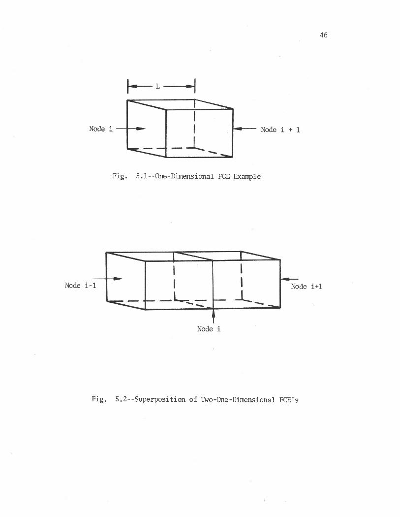
To obtain the solution to this problem by the FCE method, one

dimensional FCE's will be used as illustrated in Figure A2. For FCE a/V A

the Fa, Ta and Ka matrices are:

FCF-FCF

1-21-2

-FCEFCF.

1-21-2

1 -1-1 1

In a similar manner the matricies for FCE b are:

-2 2 ’

The superposition matrix for FCE a is obtained from Equation (3.8) as

* /\ Ta = ir t

81

Mdplane

Fig. Al--Nomenclature for Example Problem

FCE a FCE b

Fig. A2--Definition of FCE's for Example Problem

where

83

T =

It immediately follows from the above equations that

N* =1 0 0

0 1 0

Equations (3.9) and (3.10) then become

T AF* = N F =

1 0 0 1 0 0

V 1LF2j F2

0

and

K? = n* Xs if-

N*3 =

'1 o'0 1.0 0_

^ and

'0 1 O'.0 0 1.

1 -1

-1 1J

1 0 0 0 1 0

" 1 -1 O'-1 1 0. 0 0

-1O

In a similar manner the n \ S and K*3 matricies for FCE b are

Fb

Fb L 3.and

^ =0 0 0 0 2-2

L0 -2 2 .

Superposition of FCE a and FCE b is performed by Equation (3.7) as

follows:

84

F = K T

where

F = E F* = >

K = Z K* =1 - 1 0 -1 3 -2 .0 - 2 2

The temperature transformation matrix of Equation (3.12) is simply

obtained as

T = M U + J

where

M =

It then follows that

" 0 "

1_0_

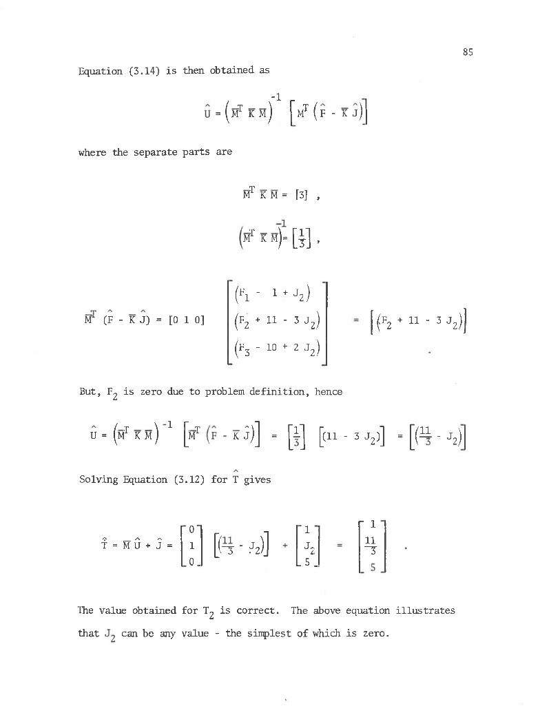
Equation (3.14) is then obtained as85

-1= (mT K m ) j V ( f - K j)

where the separate parts are

MT K M = [3] ,

m t k ma)= H •

W (F - K J) = [0 1 0]

(Fi- 1 + J2)(p2 * 11 - 3 J2)

(F3 - 10 + 2 J2)

(F2 * 1 1 - 3 J2)]

But, F2 is zero due to problem definition, hence

U ■ (mT K m) 1 [mT (i -K 5)] - [I] [(11 - 3 J2)] = [(ii - J2)

Solving Equation (3.12) for T gives

^ A A

T = H U + J =O'10

[jfT " ̂ 2)]1J.1L 5 _

r 111T

The value obtained for T2 is correct. The above equation illustrates

that can be any value - the simplest of which is zero.

86

Equation (3.11) for F then gives

-8/3F = K T = 0

+8/3

which yields the correct values for F^ and F ^ .

Example problem II

For the plate illustrated in Figure A1 the backside of plate b

and the mid plane temperature are to be obtained as a function of time.

The backside of plate b is perfectly insulated. At time zero the solid

has a constant temperature of 1°F except that the outside of plate a is

suddenly constrained to be 10°F. Both plates have a conductivity of 1

Btu/hr-ft-°F and a thickness of 1 ft. The pC product for each plate is

equal to 1 ----- . Calculations will be based on a cross sectional area£t F

of 1 ft . Two identical FCE's will be used. The nomenclature for the

two FCE's is the same as used in the last problem (see Figure A2).

The exact solution given for this problem is from Chart 2 of the

Temperature Response Charts by Schneider. For the FCE method the non

conduction heat flux vector (Equations (4.1) and (4.5)) is

However, R and E are null due to the definition of the problem. FromA A

Equations (4.3) and (4.6) it follows that the B and D vectors are

F = R + B + E + D .

B100

where87

— 3. 7=b

and

r p C V

c* =a a a

~ZAP--- 0 _

1 M O --

-1

p C V0 a a a

■ Zap 1-- o h-*

1 _ where AP = 2, hence the overall C matrix is

1 0 00 2 00 0 1

F of equation (4.16) was given as

FS = $ (H T, + B + E)p+1 + (l-<j>) (H Tm + B + E) - H T - K T)p + (C T) .

A

But H and E are both null and the conductance matrix K is ob­

tained by superposition as

K = Kt + $

" FCFl-2 -Fc f i_2" 1 -1

; f c f i -2 FCFl-2. -1 1

where

88

to give

K =1 - 1 0 -1 2 -1 0 - 1 1

The K5 matrix of Equation (4.16) was given as

K5 = [cj> (H + K) + c]P+1

and the T matrix as

Xs = TP+1

The overall equation for the system

then becomes

FS = Xs TS

_ »« «

B1 X1 - 1 0 T1 1 0 0 T1

0 + (1-40 . 0 - -1 2 -1 T2 - + i 0 2 0 T2•»

0P+1

0 0 - 1 1 LT3J■ P

0 0 1 ,T3 JJl

• -

1 -1 0 1 0 0 "Tl". <), -1 2 -1 + 0 2 0 *

T20 -1 1 _0 0 1 _ p+1 3_

P+1

Carrying out the indicated operations, the above equation becomes

89

■ “ ■ "(<f> Bx + (1-<|>) Bx + (l-<j>) ( T ^ ) + Tx\ 1+(J> -4> 0 T1

(a-*) (t x - 2 T2 * T j) * 2 T2) = -<f> 2 + 2 $ -<P T2

((1-40 CT2 - V + h )P

0 - $ l + $p + 1

_T3

With <J> = 0 (forward difference), the previous equation reduces to

'B1 + T2 1 0 0

i---rHH

T 1 + T3 = 0 2 0 TL 2

T2 0 0 1 TL 3 JLm -JP

Equation (4.17) indicates that

Ts = T , = M , U , + J +1p+1 p+1 p+1 p+1

where

'io' A "J = J2 and U =

A--1to__1

Hence, the matrix M

'0 0"M = 1 0

.0 1.

Carrying out the indicated operations, the above equation becomes

89

With <f> = 0 (forward difference), the previous equation reduces to

'Bl + T "l 2

1 0 o ___1

Tl + TX3 = 0 2 0

_T2P

0 0 1L J J p+l

Equation (4.17) indicates that

r p S _ = M U + Jp+1 p+1 p+1 p+1

where

A10

ATl 2

J = J2 and U =

' H

- J3 -

Hence, the matrix M 1S

“0 0"M = 1 0

.0 1-

Equation (4.18) was given as

V - («£**■ Vi)'1 MP+1 v ) J

The individual parts are determined as

(tf i?#)-1 -\2 t ' . i p °i.0 lj Z L 0 2 J

and

mp*i ( ^ Vi) -T1 + T3 " 2 J2

T2 " J3

Equation (4.18) then becomes

Up+1

T1 T3T + T " J 2

T9 - J7 ■ 2 3 -Jp

and Equation (4.17) becomes

T ,.1 = M x1 U ±1 + J .p+1 p+1 p+1 p+1

105 + (T3)/2 T0

Again note that ^ and could have taken on any value.

Now for tf> = 1 (backward difference), the equation for

F5 = Is Ts

reduces to

■ B1 ♦ T1- "2 -1 0 " V2 T2 = -1 4 -1 T2

1 Lhl

1___

P .0 -1 2 . _ T3.P+1

This gives for Equation (4.18) and (4.17) the following:

V i - 15 V i)'1 (hp*i ■16 W )

1 4 T2 + 2 Tl ♦ T3 - 7 J2

7 2 T0 + T, + 4 T, - 7 J7

and

/\

"10

- (4 T2 + 20 + T3)

- (2 T2 + 10 + 4 T3)

Again, note that the values of J2 and J3 are irrelevent.

For = 1/2 (mid difference), the equation for

reduces toT T 2 1

B1 + T + T1.5 -.5 0 T1

T1 T34 + T2 +4 = -.5 3 -.5 T2

T2 T3 T T 0 -.5 1.5 T3

P p+1

This gives for Equations (4.18) and (4.17) the following:

92

V i - (mp+i *■ Vi)'1 ( ^ i (?s ■ r W

217

3 T 1 + X T2 * 2 TS - T- J2

Tl + 4T2 *l'3 - 4 J3 J

IT (3 V i V n )

IT (T1 + 4T2 * I T3)v / J p

A g a in , n o t e t h a t t h e v a l u e s o f an d a r e i r r e l e v a n t .

A comparison of all the results obtained with the exact solution is

shown in Figure A3. It is of interest to note that for even such a

crude model (only two FCE's used) reasonable agreement is obtained.

Also note that <j> = 0 gives the least accurate results and that (p = 1/2

gives the best results of the three.

= M U + Jp + 1 p+1 p + 1 p+1

Fig. A3--Comparison of Results Obtained by Finite Conductance Element 1 iethod with the Exact Solution. — , Exact Solution.--#--, 0=0 (forward difference). ■ , 0=1/2 (mid difference). ▲ , 0=1 (backward difference).

VO

FINITE CONDUCTANCE ELEMENT METHOD OF

CONDUCTION HEAT TRANSFER

E. Clark Lemmon

Department of Mechanical Engineering Science

Ph.D. Degree, April 1973

ABSTRACT

The major objective of this dissertation was to develop a numerical conduction model which had the following advantages:

1. Be as simple to formulate as the standard finite difference method.

2. Be able to handle irregular boundaries with the ease of the finite element method.

3. Have the superposition advantages of the finite element method, thus requiring a minimal amount of input to use. The resulting method is termed the finite conductance element (FCE) method. Basically, the FCE method employs a discrete form of Fourier's law of heat conduction termed finite conductance factors (FCF). These FCF's are used to build a set of different FCE's. These FCE's may be con­sidered as simple conductance building blocks. The solid of interest is filled with these simple building blocks and and accounting method is developed to monitor the conduction of heat and temperature variation within each FCE in the system.

COMMITTEE APPROVAL: