October 26, 1998 Finite Element Analysis of Active Vibration Isolation Using Vibrational Power as a Cost Function Carl Q. Howard and Colin H. Hansen Department of Mechanical Engineering, The University of Adelaide, South Australia 5005, Australia TOTAL NUMBER OF PAGES 35 NUMBER OF FIGURES 23 NUMBER OF TABLES 1 SEND TO: Scientific Editor: Prof. Malcolm Crocker International Journal of Acoustics and Vibration Department of Mechanical Engineering 201 Ross Hall Auburn University AL 36849 - 5341 USA phone: 334-844-3310, fax: 334-844-3306 e-mail: [email protected]Subject Classification: 8.10 Active Reduction of Vibration 1
Transcript
October 26, 1998
Finite Element Analysis ofActive Vibration Isolation
Using Vibrational Power as a Cost Function
Carl Q. Howard and Colin H. HansenDepartment of Mechanical Engineering, The University of Adelaide,
South Australia 5005, Australia
TOTAL NUMBER OF PAGES 35NUMBER OF FIGURES 23NUMBER OF TABLES 1
SEND TO: Scientific Editor: Prof. Malcolm CrockerInternational Journal of Acoustics and VibrationDepartment of Mechanical Engineering201 Ross HallAuburn UniversityAL 36849 - 5341USAphone: 334-844-3310, fax: 334-844-3306e-mail: [email protected]
Subject Classification: 8.10 Active Reduction of Vibration
1
Abstract
An active vibration isolation system comprising of a simply supported beam and a rigid mass mounted
on an active isolator is analyzed using Finite Element Analysis. The cost function which is minimized
is the vibrational power transmitted from the vibrating mass into the beam. The analysis shows that
moments can generate negative power transmission values along a translational axis. It is shown that
a control strategy which minimizes the power transmission along a translational axis and neglects the
power transmission due to moments can produce higher beam vibration levels than without control.
It is shown by example that the minimization of squared acceleration or squared force in the ver-
tical direction at the base of the isolator, performs nearly as well as the minimization of total power
transmission (along translational and rotational axes).
It is shown that the cost function of translational power transmission along the vertical axis can have
negative values, when rotational moments are present. In these situations, the cost function of squared
power transmission along the vertical axis will have a locus of filter weights where the squared power
transmission is zero along the vertical axis. The optimum set of filter weights corresponding to the
minimization of squared acceleration or squared force along a vertical axis, is a point which lies on this
locus. It is shown that a point exists on this locus, where the control effort is also minimized. At this
point, the control effort is less than that required when the squared acceleration or squared force along
the vertical axis is minimized. However, at the point where squared power transmission along the vertical
axis and the control effort is minimized, the total power transmission is not necessarily minimized and
generally not as small as achieved by just minimizing squared force or squared acceleration in the vertical
Z direction at the base of the isolator.
Two adaptive control algorithms are suggested for finding the optimum filter weights which minimize
the squared power transmission and the control effort. The first algorithm uses Newton’s method to
minimize the control effort by moving the filter weights along a constant power level on the error surface
without causing an increase in the residual error. A second method is suggested which alternates the
filter weight updates between a partial leaky filtered-x LMS algorithm and the standard filtered-x LMS
algorithm. This results in a zigzag path of the filter weights and a slightly greater residual error than the
first algorithm.
2
I. INTRODUCTION
In a typical vibration isolation system, a vibrating rigid body provides a power source which is
dissipated by an isolator and a support structure. Vibrational power is transferred by translational forces
and rotational moments. It has been shown in the literature that in the calculation of vibrational power
transmission (or structural intensity) at the intersection of an active isolator and support structure, the
inclusion of power from rotational moments can act to cancel the contribution of power from translational
forces.1,2 Power transmission from moments is converted into translational power transmission upon
reflection at the supports, and interacts with the translational power transmission due to translational
forces. This can result in negative values of vibratory power transmission (that is, power reversal) along
a translational axis.
Previous experimental work reported by the authors3 showed that for a vibrating mass actively isolated
from a simply supported beam, there were frequencies for which the vertical power transmission under
active control was worse than for the passive case. An accelerometer and force transducer combination
was used to measure the power transmission from the isolator into the beam. A heterodyning technique
was used to combine velocity and force signals at the base of the isolator, into a signal which was
proportional to the vertical vibrational power transmission at the driving frequency.3 It was reported
that power transmission from moments was suspected to be the cause of the measurement of negative
power transmission.
In experimental work on active vibration isolation, the measurement of moments is often omitted
because their contribution is considered negligible or because of the unavailability of suitable transducers.
This paper demonstrates through Finite Element Analysis that a control strategy which minimizes the
power transmission into a support structure, when the power transmission due to small moments is
neglected, can result in total vibrational power levels greater than without control.
Gardonio4,5 has analyzed the power transmission of a vibrating rigid mass isolated from a plate using
two active mounts. Gardonio showed that minimization of the out of plane component of power, when
power transmission due to moments was omitted, caused a ”power circulation” phenomena, where power
was drawn into the plate and then re-absorbed by the active mounts. Power circulation caused greater
vibration levels in the plate than without active control. Gardonio’s work used two different types of
cost functions. The first was the out of plane power transmission, which was capable of negative values
and the second was the weighted sum of the out of plane squared acceleration and squared force, which
is positive definite. The weighting factor was applied to the squared force error signal so that it was the
3
same order of magnitude as the squared velocity signal. In this case, the weighting factor was chosen to
be the square of the point mobility of the receiving structure. Gardonio reported that the second cost
function gave better results than the first. This result is not surprising as the second cost function is
always positive and by the definition of power transmission, if the squared acceleration or squared force
is reduced to zero, then the power transmission along a vertical (out of plane) axis is also reduced to zero.
The surprising result was that the second cost function gave results close to the minimization of total
power transmission, except at a few frequencies where active isolation was worse than passive isolation.
The filtered-x LMS (FX-LMS) algorithm is a gradient descent method which minimizes the mean
squared value of an error signal.6 Most researchers use the FX-LMS algorithm to minimize a cost
function based on the force or acceleration at a point on the receiving structure. It is shown here that
the minimization of squared acceleration or squared force along the vertical axis gives results which
nearly match the results obtained by the minimization of total power transmission, except at rotational
resonances where the value of total power transmission under active control can be greater than that
corresponding to the passive case.
Structural or acoustic intensity cost functions presented in the literature7–10 attempt to minimize the
signed value of structural intensity. These algorithms are based on a cost function which consists of the
total power transmission determined by measuring along a sufficient number of axes so that the cost
function is positive definite. If negative values of measured power transmission are possible as a result of
omitting the contribution of power transmission from motion around rotational axes, the algorithms will
converge to the negative value and could result in total power transmission (and thus overall structural
vibration) levels which are greater than without control.
It follows that a better cost function to minimize is the absolute or squared value of power transmission
rather than the signed value of power transmission. In the work presented here, it is shown that the
minimization of the squared power transmission will not cause the power circulation phenomena reported
by Gardonio.4,5 As the possibility exists for negative values of power transmission, the error surface of
the squared power transmission plotted as a function of control filter weight values, no longer exhibits a
unique global minimum; instead a locus exists where the power transmission is zero. It is shown that a
control force exists which lies on this locus of zero power transmission and will and less control effort is
required than when squared acceleration or squared force are minimized; however it remains to be seen
if this control force also minimizes the total power transmission.
To calculate the optimal control force, a cost function is proposed which uses the method of Lagrange
multipliers to combine the vibrational power transmission and a control effort term. This results in a
4
cost function that has a unique global solution. The method of Lagrange multipliers is a useful tool for
modelling purposes, but it is not easily implemented in real time because the process involves calculating
a solution to a system of non-linear equations. It is preferable in practice to implement an adaptive
algorithm such as the leaky-LMS algorithm.
Two adaptive algorithms are developed here to minimize the squared power transmission and the
control effort. The first uses Newton’s method6 to measure the gradient of the mean linear vibrational
power transmission. The gradient calculation is used to adapt the filter weights along the normal to the
gradient. The second method is based on the leaky FX-LMS algorithm.6 The filter updates alternate
between a partial leaky FX-LMS algorithm and the standard FX-LMS algorithm, which results in a
zigzag path of the cost function when plotted as a function of the filter weight values.
This paper examines the power transmission for several cost functions when the power transmission
due to moments is omitted. The cost function based on the minimization of the total power transmission
completely describes all the mechanisms of power transmission and is the datum to which all other
proposed cost functions will be compared.
II. THE FINITE ELEMENT METHOD
A three dimensional Finite Element Model (FEM) was constructed using the software package Ansys,
to describe the experimental arrangement presented in a previous paper,11 as shown in Fig. 1.
Force andAccelerationTransducers
Primary Forceand Moment
Top Mass
Lower Mass
Simplysupportedbeam Actuator
x
yz
Figure 1: Schematic of the 3-D beam system.
A script file which contained Ansys instructions and a FORTRAN program was used to determine
the optimum control forces. The details of the steps involved are described in the following sections.
The method is similar to that used previously12,13 in which displacement was the cost function to be
5
minimized. However the method presented here differs from the previous work in that the cost function
used is the vibrational power transmission into the support structure and also, the effects of moments on
the cost function are investigated.
The program followed the steps outlined below.
A. Definition of the problem
A FEM is constructed of the system shown in Fig. 1, with node locations defined for the primary
forces, control forces and error sensors.
The advantage of using FEA techniques is that any structure can be used with any primary, control
and error sensor locations.
The FEM constructed for this case is shown in Fig. 2. The beam was model used 121 shell elements
(SHELL63), 6 spring elements (COMBIN14) for the vibration isolator (the vertical line in the centre
of Fig. 2) and 2 mass elements (MASS21) to model the top and lower masses (cannot be seen in the
figure). The model used 6 spring elements to account for the 6 axes of vibration, however in this paper,
XY
Z
Figure 2: The finite element model.
only vibration along the vertical axis (Z) and rotations around the θy axis are investigated. The control
actuator is orientated along the vertical Z axis and is attached to the top and lower masses. A positive
primary force is assumed to act upwards along the Z axis and a positive control force is assumed to be
a tensile force, which acts against the primary force.
For the general case, there are np primary forces or moments acting on the structure, nc control forces
which counter-act the primary forces and there are ne nodes on the structure which are used to measure
the displacement and force. These nodes will be called the error sensors.
6
B. System identification
The response of the system is determined by measuring the influence coefficients14 for the primary
and control forces. The effect of the primary forces is investigated first. All nc control forces and
np primary forces are set to zero except for one of the np primary forces which is set to a unit load.
The displacement and force responses are determined at each of the ne error sensors over the analysis
frequency range. This process is repeated for each of the primary forces and then each of the control
forces. The displacement and force responses are effectively transfer functions between the error sensor
and the driving force because a unit load was applied to the structure. The transfer functions are saved
to external files for use by an external FORTRAN program to determine the optimal control forces, as
described in the next section.
C. Determination of optimal control forces
The displacement and force at the ne error sensors can be described by vectors dt and ft which have
a length ne. The displacement and force vectors are given by
dt = Zdpfp + Zdcfc (1)
ft = Zfpfp + Zfcfc (2)
where fp and fc are the primary and control force column vectors of length np and nc respectively, Zij is
a transfer function between displacement or force, i, and primary or control force, j. For example, Zfc is
the transfer function matrix of dimensions (ne × nc) between the response due to the forces measured at
the error sensor and the driving control force. These definitions can be used to define the time averaged
harmonic vibrational power transmission into the structure as
Power =ω
2Im
(dH
t ft)
(3)
where the superscript H is the Hermitian transpose and ω is the angular frequency in rad/s. Substitution
of Eqs. (1) and (2) into Eq. (3) and rearrangement results in a quadratic expression in terms of the control
force qc15
Power =ω
2
(qH
c αq c + qHc β + βHq c + ci
)(4)
7
where
q c =
⎡⎢⎣
f rc
f ic
⎤⎥⎦ (5)
α = αT =12
⎡⎢⎣
ai + (ai)T ar − (ar)T
−ar + (ar)T ai + (ai)T
⎤⎥⎦ (6)
β =12
⎡⎢⎣
(bi2)
T + bi1
(br2)
T − br1
⎤⎥⎦ (7)
and the real matrices f rc , f i
c ,ar,ai,br1, · · · represent, respectively, the real and imaginary parts of the
complex matrices fc,a,b1 and b 2 and the complex constant c which are defined as
a = ZHdcZfc (8)
b1 = ZHdcZfpfp (9)
b2 = fHp ZH
dpZfc (10)
c = fHp ZH
dpZfpfp (11)
The power transmission into the system for passive vibration isolation qc = [0, 0]T is given by ωci/2. The
minimum of Eq. (4) is given by
Powermin = −ω
2
(βTα−1β + ci
)(12)
corresponding to an optimum control force vector given by
(q c)opt = −α−1β (13)
This optimum control force is calculated using a FORTRAN program which writes a file for each control
force or moment.
8
Table 1: The parameters used in the modelling.Beam length 1.500m Beam width 0.160m
Beam thickness 0.010m Isolator location 0.760mYoung’s modulus 71 GPa Moment of inertia 1.6 × 10⁻⁵ m4
Isolator stiffness kθy 216 N/rad Isolator damping cθy 140 sN/radTop mass 7.44 kg Bottom mass 7.88 kg
D. Calculation of the response for active control
The matrices of optimum control forces are loaded into Ansys and the response is determined for
a single frequency. The responses at the error sensors are recorded, along with additional measurement
points. This is saved to another file for post-processing and analysis.
E. Analysis of results
The power transmission under active isolation is calculated using the response determined in the
previous section and a Matlab script which uses Eq. (3).
III. VERIFICATION OF FEA WITH THEORY
For validation purposes, the power transmission values obtained using the finite element method of the
simply supported beam and the active isolator were compared with results obtained using a theoretical
model16 for a unit load along the vertical axis for passive and active isolation. The parameters which
were used in the model are shown in Table 1.
A unit harmonic primary force Fz = 1N was applied to the top mass along the vertical Z-axis. The
power sensors were placed between the active isolator and the simply supported beam. The control
actuator acted against the lower mass and reacted against the top mass. Figs. 3 and 4 compare the
theoretical and FEA predictions of power transmission into the simply supported beam for passive and
active vibration isolation. For the passive case illustrated in Fig. 3, the FEA predictions match the
theoretical model, which demonstrates the accuracy of the FEA modelling.
For the active case in Fig. 4 the results are close to the passive power transmission values minus 160 dB.
This can be interpreted as the control force having completely cancelled the action of the single primary
force, to within the numerical precision of the software. This result differs from the results presented
previously16 which predicted a finite power transmission for active control as a result of numerical errors.
9
0 10 20 30 40 50 60 70 80 90 100-85
-80
-75
-70
-65
-60
-55
-50
-45
-40
Po
we
r (d
B r
e 1
W)
Frequency (Hz)
TheoryANSYS
Figure 3: Comparison of theoretical and FEA predicted power transmission along the vertical Z-axis intothe beam for passive isolation of a vertical load Fz = 1N.
0 10 20 30 40 50 60 70 80 90 100-300
-250
-200
-150
-100
-50
0
Pow
er
(dB
re 1
W)
Frequency (Hz)
Passive: Theory & FEAActive: TheoryActive: FEAPassive *1e-16
Figure 4: Comparison of theoretical and FEA predicted power transmission into the beam along thevertical Z-axis for active isolation of a vertical load of Fz = 1N.
10
These errors can be corrected by reducing the size of the matrices to remove the redundant entries, as
shown previously.15
The two cases of passive and active isolation considered here verify that the FEA method is capable
of predicting values of power transmission for passive and active isolation.
IV. PASSIVE ISOLATION OF A COMBINED FORCE AND A MOMENT
Fig. 5 shows the power transmission along the vertical Z-axis and around the rotational θy axis for
passive isolation of a unit harmonic load Fz = 1N acting along the vertical Z-axis, with a rotational
moment around the θy axis of My = 0.005Nm. A rotational moment can be generated by misalignment
of the primary force with the centroid of the top mass. The peaks in Fig. 5 correspond to resonance
frequencies of the combined beam-isolator system. Fig. 5 shows that negative power transmission occurs
in the frequency range of 35-39 Hz and 92-100Hz. In this case a 5mm misalignment of the primary shaker
with the centroid of the top mass generated the required rotational moment. The phenomenon also exists
for 2mm of misalignment, which is likely to occur in practice. For passive vibration isolation, the total
0 20 40 60 80 100−120
−110
−100
−90
−80
−70
−60
−50
−40
Frequency (Hz)
Pow
er (
dB r
e 1W
)
Z axis: positive Z axis: negative θy axis: positiveθy axis: negativeTotal power
Figure 5: Power transmission along the vertical Z-axis and around the rotational θy axis for the passiveisolation of a combined load of Fz = 1N and moment My = 0.005Nm.
vibrational power transmitted, Pt, from the isolator must be absorbed in the receiving structure. The
total power transmission, Pt, comprises of power transmission by translational forces and velocities Pf
and also by moments and rotational velocities Pm so that
Pt = Pf + Pm (14)
11
From the conservation of energy principle, the total power transmission must be greater than zero Pt > 0
as power is absorbed by the receiving structure; however negative values of power transmission, Pf < 0,
along the vertical Z-axis can occur if the power due to rotational moments (Pm) is greater than the
magnitude of the power transmitted by translational vertical forces, i.e. Pm > ‖Pf‖ > 0. Fig. 5 shows
the relative contributions of the power transmission along the vertical Z-axis and along the θy axis
compared with the total power transmission for a combined load of a force along the vertical axis of
Fz = 1N and a rotational moment around the θy axis of My = 0.005Nm. At every frequency, the axis
which has the greatest absolute value of power transmission has a value that is always positive. For
example, at 38Hz the value of power transmission along the Z-axis is -75dB in a negative sense, flowing
out of the beam. Around the θy axis the power transmission is -69dB in a positive sense, flowing into the
beam. The magnitude of power transmission along the θy axis is greater than the magnitude of power
transmission along the Z-axis which confirms that the total power transmission will always be positive
(in Fig. 5 it is -70dB in a positive sense), even though negative power transmission can occur along a
particular axis.
Negative values of power transmission along an axis can occur when wave type conversion has occurred
at the boundary conditions on a structure. If one considers an undamped semi-infinite beam terminated
with a simple support, a wave traveling towards the simple support will be reflected. The simple support
will restrict the displacement of the beam along the vertical Z-axis, but allow free rotation around the
θy axis. When an incident wave is generated by the application of a vertical force to the beam, the wave
will travel along the beam towards the simple support. The displacement of the beam will be mainly
along the vertical Z-axis with little displacement around the θy axis. When the wave reaches the simple
support, a reaction force will be generated and a reflected wave will return along the beam which will
have displacement mostly along the vertical Z-axis and thus no wave conversion will have occurred. On
the other hand, when a rotational moment is applied to the beam, a wave will travel along the beam
towards the simple support. The displacement of the beam will be mainly around the θy axis and as a
result of coupling, will cause displacement along the vertical Z-axis. When the wave reaches the simple
support, the support is free to rotate around the θy axis and is unable to generate a reaction moment.
As the incident wave energy must be conserved, the reflected wave energy appears in the form of a
backwards traveling wave with displacement mostly along the vertical Z-axis. This mechanism of wave
type conversion causes the summation of incident power along the vertical Z-axis and the reflected power
from the conversion of power transmitted by moments into power transmission along the vertical Z-axis,
to result in negative values of power transmission along the active isolator Z-axis.
12
Fig. 6 shows the total power transmission into the beam for three load cases. The first is a force
0 20 40 60 80 100−140
−120
−100
−80
−60
−40
Frequency (Hz)
Tot
al P
ower
(dB
re
1W)
Fz=1N and My=0.005NmFz=1N My=1Nm
Figure 6: Total power transmission for three load cases of Fz = 1N, My = 0.005Nm and the combinedload of Fz = 1N and My = 0.005Nm.
Fz = 1N, along the vertical Z-axis, the second is a rotational moment My = 0.005Nm, around the
θy-axis and the third is a combined load of Fz = 1N and My = 0.005Nm. Power transmission into the
beam is calculated using Eq. (3), which takes the imaginary part of the product of the conjugate of the
displacement vector with the force vector. Hence the power transmission for the third load case, the
combined translational force and rotational moment load, is not the sum of the power transmission from
the translational force and moment acting separately. At 35Hz, the total power transmitted into the
beam for the combined load case is less than that transmitted for each of the other two load cases, which
means that the power transmitted by rotational moments has a cancelling effect on the power transmitted
by translational forces.
V. ACTIVE ISOLATION OF COMBINED FORCE AND MOMENT
It was shown in Fig. 4, that when a vertical load, Fz = 1N, along the Z-axis was applied to the
structure, only positive values of power transmission are possible. The cost function based on the power
transmission is always positive and has a unique global solution for the control force so that the control
actuator is able to completely cancel the vibration.
When a rotational moment is also applied to the primary load in addition to the vertical force, so that
negative values of power transmission along a vertical axis are possible, the cost function is not always
positive and interesting results can occur. In the following sections, several cost functions are compared
13
according to their ability to reduce the total vibrational power transmission into the beam.
A. Minimization of Squared Acceleration and Squared Force
Most researchers use a cost function based on the squared acceleration because sensors can be eas-
ily attached to the receiving structure and the acceleration signal is suited for use with the FX-LMS
algorithm. The error surfaces of the cost functions based on the squared acceleration or squared force
at the base of the isolator are positive definite and have a unique global minimum. Gradient descent
algorithms, such as the FX-LMS algorithm, will converge to this global minimum. Fig. 7 shows the total
power transmission into the beam for passive isolation and at the unique global minimum for five active
isolation cases which are the minimization of the squared acceleration along the vertical Z-axis, the sum
of the squared acceleration along the Z axis and the squared rotational acceleration around the θy axis,
the squared force along the vertical Z-axis, the sum of the squared force along the vertical Z-axis and
the squared rotational moment around the θy axis, and the total power transmission along the Z and θy
axes. It can be seen that at 35Hz, for the minimization of the squared acceleration or force along the
0 20 40 60 80 100−140
−120
−100
−80
−60
−40
Frequency (Hz)
Tot
al P
ower
(dB
re
1W)
Passive Active: Accel2 in Z axis Active: Accel2 in Z and θy axisActive: Force2 in Z axis Active: Force2 in Z and θy axisActive: Total Power
Figure 7: Total power transmission for active control of a combined load Fz = 1 N and My = 0.005 Nmusing cost functions which minimize the squared acceleration along the Z-axis, sum of squared accelera-tions along Z and around the θy axes, squared force along the Z-axis, sum of the squared forces alongthe vertical Z-axis and around the θy axes and the total power transmission.
vertical Z-axis, the total power transmission for active control is greater than for passive isolation. At
35Hz there is a rotational resonance, which cannot be adequately controlled by the control actuator which
is orientated along the vertical Z-axis. One would expect that at this frequency, active control is unlikely
to improve the vibration isolation, but the active case should not be worse than the passive isolation case.
However as shown in Fig 7, the active control case is indeed worse than the passive case. This is because
14
some of the vibrational power along the vertical Z-axis can be used to cancel the power transmission
along the θy axis. The minimization of squared acceleration or squared force along the vertical Z-axis
reduces the power transmission along the vertical Z-axis to zero thus negating its cancelling effect on the
power transmission along the θy axis. Hence the total power transmission for active control at 35Hz is
greater than for passive isolation.
The active control of squared acceleration along the vertical Z-axis results in values of total power
transmission which are close to those obtained for the minimization of the total power transmission,
except at resonance frequencies for motion around the rotational θy axis. It would seem reasonable
that an improvement in vibration isolation could be obtained by minimizing the sum of the squared
accelerations along the vertical Z-axis and around the rotational θy axis. However, as shown in Fig. 7,
the active isolation performance using a cost function of the sum of the squared accelerations along the
vertical Z-axis and around the rotational θy axis is worse than using a cost function of the squared
accelerations along the vertical Z-axis, except at resonance frequencies for rotational motion around the
θy axis. Active control has attempted to reduce the rotational vibration around the θy axis at the expense
of increasing the vibration along the vertical Z-axis. This increases the total power transmission compared
to when the squared acceleration along the Z-axis is minimized. When the squared acceleration along
the vertical Z-axis is minimized, the squared acceleration and the power transmitted along the vertical
Z-axis is reduced to zero, which leaves the power transmitted along the θy axis as the only contributor to
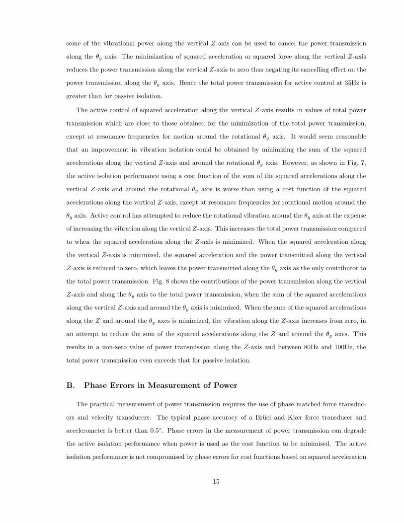
the total power transmission. Fig. 8 shows the contributions of the power transmission along the vertical
Z-axis and along the θy axis to the total power transmission, when the sum of the squared accelerations
along the vertical Z-axis and around the θy axis is minimized. When the sum of the squared accelerations
along the Z and around the θy axes is minimized, the vibration along the Z-axis increases from zero, in
an attempt to reduce the sum of the squared accelerations along the Z and around the θy axes. This
results in a non-zero value of power transmission along the Z-axis and between 80Hz and 100Hz, the
total power transmission even exceeds that for passive isolation.
B. Phase Errors in Measurement of Power
The practical measurement of power transmission requires the use of phase matched force transduc-
ers and velocity transducers. The typical phase accuracy of a Bruel and Kjær force transducer and
accelerometer is better than 0.5◦. Phase errors in the measurement of power transmission can degrade
the active isolation performance when power is used as the cost function to be minimised. The active
isolation performance is not compromised by phase errors for cost functions based on squared acceleration
15
0 20 40 60 80 100−160
−140
−120
−100
−80
−60
−40
Frequency (Hz)
Pow
er (
dB r
e 1W
)
Passive Active: Power along Z axis Active: Power along θy axis Active: Power along Z and θy axes
Figure 8: The components of the total power transmission when the sum of the squared accelerationsalong the vertical Z-axis and around the θy axis is minimized.
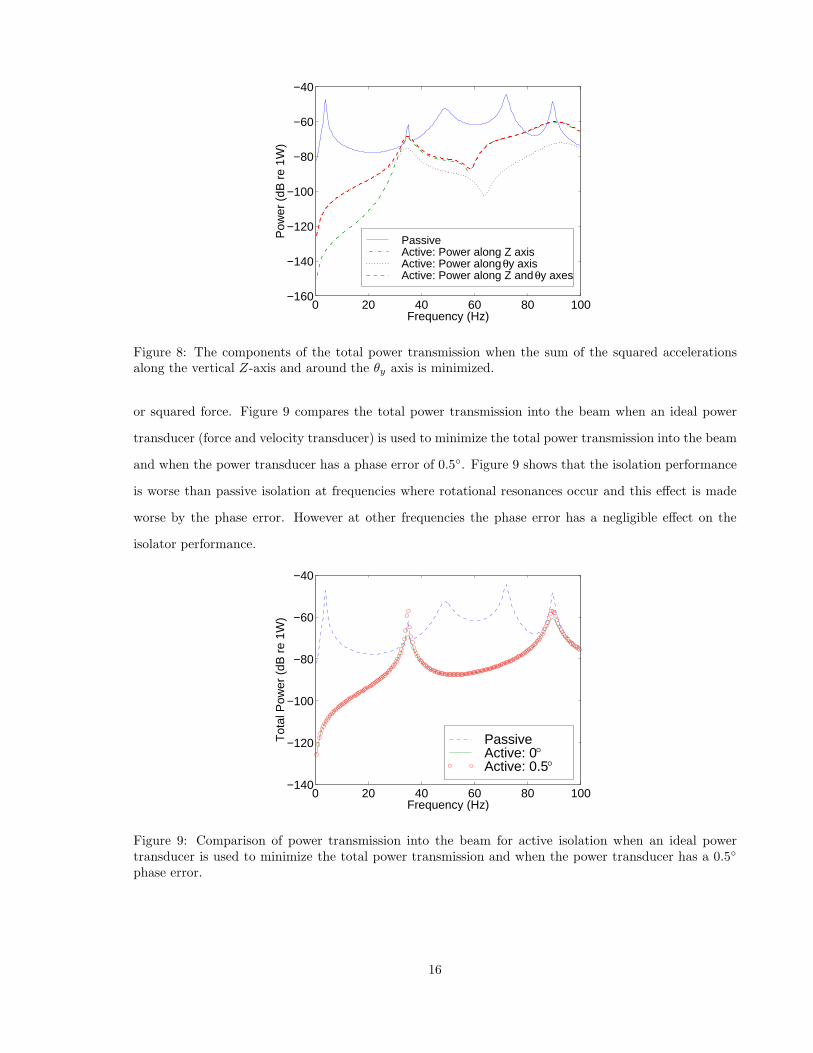
or squared force. Figure 9 compares the total power transmission into the beam when an ideal power
transducer (force and velocity transducer) is used to minimize the total power transmission into the beam
and when the power transducer has a phase error of 0.5◦. Figure 9 shows that the isolation performance
is worse than passive isolation at frequencies where rotational resonances occur and this effect is made
worse by the phase error. However at other frequencies the phase error has a negligible effect on the
isolator performance.
0 20 40 60 80 100−140
−120
−100
−80
−60
−40
Frequency (Hz)
Tot
al P
ower
(dB
re
1W)
Passive Active: 0° Active: 0.5°
Figure 9: Comparison of power transmission into the beam for active isolation when an ideal powertransducer is used to minimize the total power transmission and when the power transducer has a 0.5◦
phase error.
16
C. Minimization of Signed Power Transmission
Figs. 10, 11 and 12 show the power transmission into the beam along the vertical Z-axis, along
the rotational θy axis and the total power transmission respectively, for the cases of passive and active
isolation when the error criterion to be minimized is the signed translational power transmission along
the vertical Z-axis and when the error criterion is the total power transmission along the vertical Z-axis
and along the rotational θy axis.
0 20 40 60 80 100−180
−160
−140
−120
−100
−80
−60
−40
Frequency (Hz)
Pow
er a
long
Z a
xis
(dB
re
1W)
Passive: Positive values Passive: Negative values Active: minimizing total powerActive: minimizing transl’nal power along Z axis
Figure 10: Comparison of passive and active power transmission along the Z-axis using translationalpower along the vertical Z-axis as the error criterion and the total power transmission (sum of poweralong the Z and θy axes) as the error criterion respectively.
0 20 40 60 80 100−160
−140
−120
−100
−80
−60
−40
Frequency (Hz)
Pow
er a
long
θy
axis
(dB
re
1W)
Passive: Positive values Passive: Negative values Active: minimizing total powerActive: minimizing transl’nal power along Z axis
Figure 11: Comparison of passive and active power transmission along the θy axis using translationalpower along the vertical Z-axis as the error criterion and the total power transmission (sum of poweralong the Z and θy axes) as the error criterion.
17
0 20 40 60 80 100−130
−120
−110
−100
−90
−80
−70
−60
−50
−40
Frequency (Hz)
Tot
al P
ower
(dB
re
1W)
Passive Active: minimizing total powerActive: minimizing transl’nal power along Z axis
Figure 12: Comparison of passive and active total power transmission using translational power alongvertical Z-axis as the error criterion and the total power transmission (sum of power along the Z and θy
axes) as the error criterion.
In Fig. 10 it can be seen that the power transmission along the vertical Z-axis for active isolation is
negative at all frequencies when the error criterion is the power transmission along the vertical Z-axis.
This is because the active control algorithm attempts to make the power transmission along the Z-axis
as negative as possible. The mechanism for achieving this is that the isolator maximizes the power
transmission due to moments, which is reflected from the beam termination and returns as negative
power along the Z-axis. After the moment power has been reflected at the beam simple supports and
returned to the isolator as translational power, the isolator absorbs power, effectively drawing power from
the support structure, rather than allowing it to dissipate through structural damping. The isolator is
able to influence the moment power transmission as the moment power is coupled to the translational
power.
Fig. 11 shows that active isolation using a single sensor measuring power along the vertical Z-axis
results in power transmission values along the θy axis greater than for the passive case, for the same
reasons as outlined above. In this case, active control has increased the total power transmission into the
support structure compared to passive isolation, which can be seen in Fig. 12.
From Fig. 12, it can be seen that just minimizing power along the vertical Z-axis can lead to increases
in the total power transmission over a substantial frequency range. However, minimizing power along
both vertical Z-axis and θy axis results in a small positive power transmission at all frequencies which is
a substantial reduction over the passive case.
Several methods exist for the minimization of structural and acoustic intensity7–10,17–19 which are
18
applicable to the minimization of power. All of these methods are based on a gradient descent algorithm
to determine optimal filter coefficients which minimize the cost function. If the cost function is capable
of negative values, these methods will converge to this negative value which, as shown previously, could
possibly make the vibration levels greater than for the passive case.
D. Minimization of Squared Power Transmission and Control Effort
Attempts to control the vibrational power transmission, when neglecting the power transmission
due to moments, should minimize the absolute value of power rather than the signed value, to prevent
minimization to a negative value of power transmission, which can increase total vibration levels in the
beam.
For the problem considered here, it is not feasible to minimize the absolute value of power transmis-
sion; rather the mean squared power transmission is used, thus always ensuring zero or positive power
transmission.
The load applied to the structure is a translational force Fz = 1N along the vertical Z-axis and
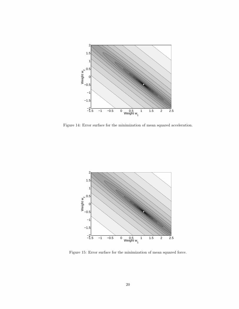
a rotational moment My = 0.005Nm around the θy axis at a frequency of 50 Hz. The error surfaces
representing cost functions of mean squared power, mean squared acceleration and mean squared force,
along the vertical Z-axis, using two filter weights, are shown in Figs. 13, 14 and 15 respectively. Black
−1.5 −1 −0.5 0 0.5 1 1.5 2 2.5−2
−1.5
−1
−0.5
0
0.5
1
1.5
2
Weight w1
Wei
ght w
2
Figure 13: Error surface for the minimization of mean squared power.
shading indicates squared values close to zero.
The control effort is the amount of mechanical power that the control actuator exerts on the structure.
In these figures with filter coefficients as the axes, the control effort can be thought of as the length from
19
−1.5 −1 −0.5 0 0.5 1 1.5 2 2.5−2
−1.5
−1
−0.5
0
0.5
1
1.5
2
Weight w1
Wei
ght w
2
Figure 14: Error surface for the minimization of mean squared acceleration.
−1.5 −1 −0.5 0 0.5 1 1.5 2 2.5−2
−1.5
−1
−0.5
0
0.5
1
1.5
2
Wei
ght w
2
Weight w1
Figure 15: Error surface for the minimization of mean squared force.
20
the origin of the filter coefficient axes to the current filter weights. Shorter lengths mean lower control
effort.
The error surface for power is different from that for the other two cost functions because there is a
dark ring which indicates a locus of zero power transmission. Inside the dark ring, the power transmission
values are negative, which when squared become positive, resulting in an error surface which has the shape
of an inverted bowl. It can be seen that the minimum error for squared acceleration and squared force,
shown in Figs. 14 and 15 by a white dot, both lie on the locus of zero power transmission. From Fig. 13
it can be seen that there is a set of filter weights which will not minimize the squared acceleration or
squared force but will give zero power transmission and will require less control effort. This means that a
solution exists which requires less energy supplied to the control actuators than required when trying to
minimize the squared acceleration or squared force, and will still minimize the power transmission along
the vertical Z-axis. It remains to be seen if this also minimizes the total power transmission. This will
be investigated in the following sections.
A numerical simulation was conducted using Matlab to demonstrate the effect of omitting the power
contribution from moments. A standard FX-LMS algorithm was used to determine a control force which
lay on the locus of zero power transmission. It can be seen from Fig. 13 that there is an infinite set of
solutions which minimize the squared power transmission along the vertical Z-axis. The behaviour of the
FX-LMS algorithm is frequently likened to a ball rolling down the sides of a bowl. When the ball reaches
the bottom of the bowl, it will cease to move. In this case, the filter coefficients will cease adaptation
when the filter weights reach the locus of zero power transmission. The final set of filter coefficients is
determined by the initial conditions of the adaptive filter. Referring to Fig. 13, if the initial value of
filter coefficients were [w1, w2] = [2, 1], then the adaptation would converge on the top side of the ring
near [w1, w2] = [1.25,−0.5]. If the initial value of filter coefficients were [w1, w2] = [−1,−1.5], then the
adaptation would converge on the lower side of the ring near [w1, w2] = [0.1, 0.1].
A control strategy is needed which will adaptively determine the optimum set of filter weights which
minimizes the vibrational power transmission as well as the control effort.
E. Methods to Minimize Control Effort
The ideal control algorithm should minimize the total power transmission into the system using the
minimum amount of control effort. If the total power transmission is not measured, because of difficulties
in measuring the power transmission around rotational axes, then an alternative cost function needs
to be found which will perform in a similar manner. One possibility is to minimize the absolute power
21
transmission along the vertical Z-axis and simultaneously minimize control effort. Graphically this would
mean that the control force would be on the locus of zero power transmission and as close as possible to
the origin of the filter coefficient axes.
The following sections discuss an analytical method for calculating a solution which will minimize
the control effort with the constraint that the power transmission is zero along the vertical Z-axis. Two
adaptive algorithms to implement the analytical method in real time are also discussed.
1. Method of Lagrange Multipliers
The method of Lagrange multipliers20 is useful for satisfying the minimization of both the control effort
and power transmission along the vertical Z-axis. The method has been mainly used in the literature
to minimize a cost function with the constraint that the control effort is limited. This prevents control
actuators from over exertion. For this case the cost function is the reverse of the typical problem, so
that control effort is minimized, with the constraint that the optimum control force must lie on the locus
of zero power transmission. The minimization of a squared cost function such as squared pressure or
squared acceleration, has been considered in the literature,21,22 however the minimization of squared
power transmission and control effort is more complicated. The cost function J(λ,Fc) becomes
J(λ,Fc) = FHc Fc + λ
ω
2
(FH
c αFc + FHc β + βHFc + ci
)(15)
where λ is the Lagrange multiplier. Proceeding in the usual manner of equating the gradient of the cost
function to zero results in
∂J
∂Fc= Fc + λ
ω
2(αFc + β) = 0 (16)
∂J
∂λ=
ω
2
(FH
c αFc + FHc β + βHFc + ci
)= 0 (17)
Re-arranging Eq. (16) for the optimum control force F∗c gives
F∗c = −
(I + λ
ω
2α
)−1
λω
2β (18)
which can be substituted into Eq. (17) and solved numerically for λ then used to solve for the optimum
control force F∗c from Eq. (18).
This method was used to determine the optimum control force for the case above. Fig. 16 shows a
shaded contour plot of the logarithmic squared power transmission (i.e. 10 log10(Power2) ) into the beam
22
as a function of the real and imaginary parts of the control force along the vertical Z-axis. The contours
-1 -0.5 0 0.5 1 1.5 2-1
-0.8
-0.6
-0.4
-0.2
0
0.2
0.4
0.6
0.8
1
Control Force - Real Part
Con
trol
For
ce -
Imag
inar
y P
art
Figure 16: Error surface of power transmission for the combined load of Fz = 1 N and My = 0.005 Nm.The dark ring at the center of the figure is the locus of zero power transmission.
show constant levels of power transmission and the darker the shading, the smaller is the value of power
transmission. The dark ring near the center of the figure is the locus where the power transmission is
zero. The location of the optimum control force is shown in Fig. 16 as a white dot which lies on the locus
of zero power transmission and minimizes the control effort, which is indicated by the close proximity of
the white dot to the origin of the axes.
2. Real Time Implementations to Minimize Control Effort
Real time implementation of active control is typically achieved using the leaky FX-LMS algorithm21
which removes a small amount from the filter weights with each update. The update equation is written
as
Wk+1 = (1 − α)Wk − 2µXek (19)
where α is a small leakage coefficient, µ is the convergence coefficient, Wk is the (n × 1) vector of the n
filter coefficients at time k, X is a (n× 1) vector of past reference signal values and ek is the error signal
value at time k.
The leakage coefficient α has the effect of moving the weight vector directly towards the origin. Using
the analogy again of a ball rolling inside a bowl to describe the behaviour of the LMS algorithm, the
adaptation halts when a balance is found between the effect of the first term in Eq. 19, which causes the
23
ball (filter weights) to climb up the edge of the bowl and the second term in Eq. 19, which causes the ball
(filter weights) to approach the bottom of the bowl. The equilibrium point is always on the side closest
to the origin, slightly above the bottom of the bowl and results in a slight increase in the residual error.
When α is set to a large value the effect on the control performance is to limit the control effort, with
a corresponding large increase in the residual error. When α is set to a small value in a multi-channel
control system, it has the effect of reducing the control effort directed to modes which require a great
deal of effort but whose control results in only a small reduction in the cost function.21
An improved algorithm would minimize the cost function, and minimize the magnitude of the filter
weights, without increasing the residual error. This can be achieved with an FX-LMS algorithm and by
updating the filter weights so that the error moves along the normal to the gradient of the error surface.
With each update of the filter weights, the magnitude of the cost function remains the same; however
the magnitude of the filter weights change.
To calculate the normal to the error surface, initially the gradient of the error surface is determined.
The FX-LMS algorithm approximates the gradient of the squared error surface as 2Xek. This set of filter
weights can be thought of as an incremental vector which when added to the current filter weights will
cause the magnitude of cost function to reduce. In 2-dimensional geometry, if a vector is given by [x, y],
then the normal to this vector is given by [−y, x]. This property can also be applied to an incremental
vector of a two tap weight FIR filter, so that when the incremental vector is added to the current set
of two filter weights, it will cause the magnitude of the cost function to remain at the same value, but
change the magnitude of the filter weights.
There is an inherent problem in using the FX-LMS algorithm to determine gradient of the cost function
so that the normal to the error surface can be calculated. As the gradient approaches zero the step size in
the normal direction will also decrease and will halt the adaptation towards the minimum control effort.
The leaky FX-LMS algorithm avoids premature halting of the progress towards the minimum control
effort by maintaining an increased residual error, compared with the standard FX-LMS algorithm, so
that the gradient of the cost function has a non-zero value.
An alternative method is to calculate the gradient of the mean linear error using Newton’s method.6
For this problem, as the mean squared error approaches zero, the gradient of the mean linear error will
have a non zero value.
The problem becomes more complicated for a general n-dimensional filter problem. A method is
required to calculate the normal to the n-dimensional gradient and this is discussed in the next section.
24
3. Proposed Algorithm Using Newton’s Method
Filter updates occur by calculating a new set of filter weights at time k + 1 by adding an incremental
value to the current filter weight at time k. This is mathematically expressed as:
w1(k + 1) = w1(k) + ∆w1
w2(k + 1) = w2(k) + ∆w2
...
wn(k + 1) = wn(k) + ∆wn (20)
The power transmission at time k is determined from the set of filter coefficients Wk = [w1, w2, · · ·wn].
After the filter update occurs, the change in values of filter coefficients can cause the value of power
transmission to change. The change in the mean vibrational power ∆P is given by
∆P = ∆w1∂P
∂w1+ ∆w2
∂P
∂w2+ · · · + ∆wn
∂P
∂wn(21)
where ∆wi is the change in the i th filter coefficient and ∂P/∂wi is the gradient of the mean linear power
with respect to the i th filter coefficient using Newton’s method. It can be seen from Eq. (21) that for a
filter with two tap weights (n = 2), if ∆w1 is assigned a value, then ∆w2 can be calculated such that there
is no change in vibrational power. When n > 2, a set of filter weights exist which can satisfy Eq. (21).
The control effort is typically measured by calculating the squared amplitude of the filter coefficients,
using the Euclidean norm ‖Wk‖2 = WTk Wk. Fig. 17 shows a contour map for a two filter weight
problem. A hypothetical error surface of mean linear vibrational power transmission has been drawn
P∇
P∇w
w1
2Gradient of power
Plane whichis tangentialto
U
Figure 17: Error surface for power transmission, showing the gradient of the power error surface, thegradient of the norm of the filter weights U and the plane which is tangential to the gradient of thepower.
25
with shaded contour bands indicating different values of power (darker shading indicating values closer
to zero) and dashed lines indicating constant levels of the squared norm of the filter coefficients. The
dashed lines form concentric circles centered about the origin of the filter coefficient axes. The gradient
of the squared norm of the filter coefficients is calculated as ∇‖Wk‖2 = 2Wk, which can be thought of
as an incremental vector in the direction of maximum rate of change of squared norm and is in a radial
direction away from the origin of the filter coefficient axes. The direction towards the origin is simply the
negative of this incremental vector, U = −∇‖Wk‖2 = −2Wk. This vector U can be projected onto the
n − 1 dimensional hyperplane which is normal to the gradient of the mean linear power. For example,
referring to Fig. 17, a filter with two weights (dimensionality n = 2) has the normal to the gradient of
the mean linear power as a line (dimensionality n = 1).
The normalized vector of the gradient of the mean linear power has unit length and is calculated as
P =∇P
‖∇P‖ (22)
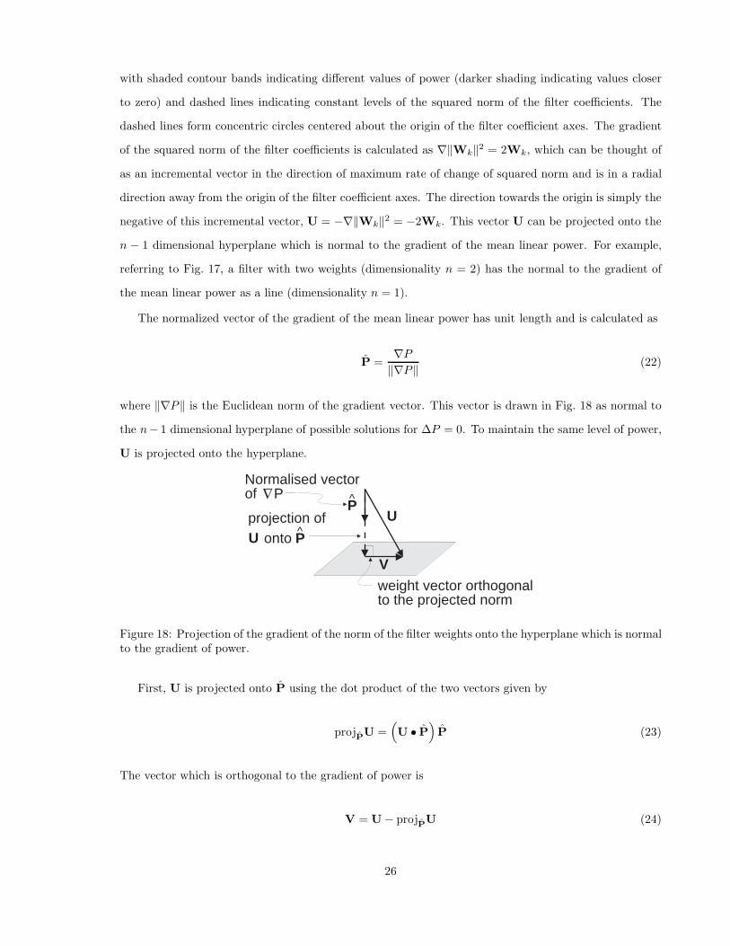
where ‖∇P‖ is the Euclidean norm of the gradient vector. This vector is drawn in Fig. 18 as normal to
the n− 1 dimensional hyperplane of possible solutions for ∆P = 0. To maintain the same level of power,
U is projected onto the hyperplane.
P∇
V
projection of onto
weight vector orthogonalto the projected norm
^P
^P
U
U
Normalised vectorof
Figure 18: Projection of the gradient of the norm of the filter weights onto the hyperplane which is normalto the gradient of power.
First, U is projected onto P using the dot product of the two vectors given by
projPU =(U • P
)P (23)
The vector which is orthogonal to the gradient of power is
V = U − projPU (24)
26
As the filter weights Wk approach the minimum norm, the norm of V becomes smaller.
To implement this algorithm in practice, each filter update performs two separate functions. First, a
standard FX-LMS algorithm is used to reduce the mean squared power transmission to zero. The filter
updates for the standard FX-LMS algorithm are given by Eq. (26). Second, this proposed algorithm is
used to reduce the control effort by updating the filter coefficients along the normal to the error surface
of the mean linear vibration power transmission.
4. Alternating Partial Leaky FX-LMS and FX-LMS Algorithm
Another way of achieving a similar result to that described in the previous section is to alternate the
filter updates between a partial leaky FX-LMS algorithm and a standard non-leakyFX-LMS algorithm.
The partial leaky FX-LMS algorithm performs the filter update given by
Wk+1 = (1 − α)Wk (25)
where α is the tap leakage coefficient (compare this with Eq. 19). The standard FX-LMS algorithm with
no leakage is given by
Wk+1 = Wk − 2µXek (26)
The partial leaky FX-LMS algorithm update, moves the filter coefficients directly towards the origin of
the filter coefficient axes which also increases the value of the cost function. The next update using the
standard FX-LMS algorithm moves the filter coefficients towards the locus of zero power transmission.
The combined effect is that the path of the filter coefficients zig-zags around the locus of zero power
transmission, eventually minimizing the norm of the filter coefficients (and thus control effort) and the
squared power transmission. The partial leaky FX-LMS algorithm causes a small increase in the residual
error compared to the FX-LMS algorithm, so that the power transmission along the vertical Z-axis is
non-zero, but this is not significant in most practical systems where other parameters determine the
maximum level of achievable control.
VI. TWO FILTER WEIGHTS EXAMPLE
The procedure which uses Newton’s method to determine the gradient of the cost function of linear
power transmission was implemented in an adaptive algorithm. The algorithm determines a control force
27
which minimizes the squared power transmission along the vertical Z-axis and the control effort for the
active isolation problem illustrated in Fig. 1.
The adaptive algorithm updated a two tap weight finite impulse response (FIR) filter. The error
surface for this problem is shown in Fig. 13. The optimization process is shown in Fig. 19 in which
the white dots show the path of the filter coefficients with each update. The initial values of the filter
−1.5 −1 −0.5 0 0.5 1 1.5 2 2.5−2
−1.5
−1
−0.5
0
0.5
1
1.5
2
Weight w1
Wei
ght w
2
Figure 19: Example of adaptation method using Newton’s method for two filter weights. The white dotsshow the filter updates.
coefficients were [w1, w2] = [1, −1]. These values were selected to demonstrate the filter coefficients
traversing along the locus of zero power transmission. Normally the filter coefficients would start at the
origin. This figure shows that the filter coefficients adapt towards the locus of zero power transmission
and then continue around the locus until the norm of the filter coefficients is also minimized. As the norm
of the filter coefficients approach the minimum value the step size decreases. At the converged solution
there is zero power transmission along the vertical Z-axis and the control effort is minimized.
The zig-zag method described in section 4 was used for the problem illustrated in Fig. 1 with a filter
having two tap weights. The adaptation was started at [w1, w2] = [1, −1] to demonstrate the zig-zag
path of the filter weights and the results are shown in Fig. 20.
The residual error is greater than that obtained using the previously described method based on
calculating the gradient of the linear power using Newton’s method. However, although the error is
greater it is still small enough to be insignificant.
Although not shown, the power transmission along the vertical Z-axis using the zig-zag method was
reduced by 50 dB. If the standard FX-LMS algorithm were used, the power transmission along the vertical
Z-axis would converge to zero.
28
−1.5 −1 −0.5 0 0.5 1 1.5 2 2.5−2
−1.5
−1
−0.5
0
0.5
1
1.5
2
Wei
ght w
2
Weight w1
Figure 20: Error surface showing adaptation using the alternating algorithm method starting at [w1, w2] =[1, −1] and zigzagging along the bottom of the bowl until the amplitude of the filter weights is minimized.
VII. FIVE FILTER WEIGHTS EXAMPLE
The isolation problem illustrated in Fig. 1 was addressed using a 5 tap weight FIR filter. Fig. 21
compares mean squared power transmission along the vertical Z-axis for the cases of passive isolation
and with the converged solutions for the cases of the FX-LMS, the leaky FX-LMS, the proposed algorithm
based on Newton’s method and the zig-zag method described in section 4.
−200
−150
−100
−50
0
Pow
er (
dB r
e 1W
)
Pas
sive
LMS
Leak
y−LM
S
Pro
pose
d
Zig
Zig
−LM
S
Figure 21: The residual power transmission at convergence for several control algorithms using a 5 tapweight FIR filter.
The methods which use the leaky FX-LMS algorithm have a small residual error, which for practical
purposes is negligible. The standard FX-LMS algorithm and the proposed algorithm based on Newton’s
29
method both converge to -195 dB which is the limit of the numerical precision of the software; hence it
indicates that zero power transmission is achieved as was done for the 2 filter weight case.
Fig. 22 shows the corresponding norm of the filter weights. The figure shows that the proposed
algorithm and the zig-zag method have a lower norm (which represents lower control forces) than the
standard FX-LMS and the leaky FX-LMS algorithm.
-25
-20
-15
-10
-5
0
no
rm W
(dB
)
Leaky
-LM
S
LMS
Pro
po
sed
Zig
Za
g-L
MS
Figure 22: The norm of the 5 filter weights at convergence for several control algorithms.
The example used to demonstrate the two new algorithms outlined in this paper is a realistic active
vibration control problem. It is possible that for more complicated error surfaces, the new algorithms
might not converge to a solution which is the global minimum of control effort, although they both will
converge to zero power transmission. Both adaptive algorithms conduct local searches to determine the
gradients of the power error surface and the norm of the filter weights. If the algorithms had been started
at [w1, w2] = [1, 1] for the two tap weight examples in Figs. 19 and 20, then the adaptation would have
halted at about [w1, w2] = [0.5, 0.3], as the power transmission would be zero and the vector V would
have converged to a local minimum. In order for the adaptation to progress towards the global solution,
the norm of the filter weights has to temporarily increase until the filter weights pass around the crest
of the locus of zero power transmission at [w1, w2] = [−1.4, 1.8] in Fig. 19. Once the filter weights
have passed this crest, the adaptation has to continue as normal until the norm of the filter weights is
minimized.
Ideally, the adaptation should ignore this local minimum and continue adaptation by following the
valley of the error surface until the global minimum of the norm of the filter weights has been reached.
However with the current approach, this cannot be guaranteed.
30
VIII. SUMMARY
The minimization of power transmission along the vertical Z-axis does not necessarily lead to the
minimization of total power transmission. If a control strategy is used which cancels the power transmis-
sion along the vertical Z-axis, such as minimization of the linear power transmission or squared power
transmission, there will be a variable amount of power transmission along the rotational θy axis which
will depend on the amplitude and phase of the control force.
It is possible to determine a set of filter weights for the 2 filter weight example from section VI, such
that the power transmission along the vertical Z-axis is zero. If a value of the first filter weight w1
is selected, then it is possible to calculate a value for the second filter weight w2 such that the power
transmission along the vertical Z-axis is zero. The corresponding control force can be written in terms
of the filter coefficients as
q c =
⎡⎢⎣
Re(w1 + w2 e−jω/ωs)
Im(w1 + w2 e−jω/ωs)
⎤⎥⎦ (27)
where ωs is the sampling frequency in rad/s, which converts the filter coefficients from the time domain
into the real and imaginary components of the control force in the frequency domain. Eq. (27) can be
substituted into Eq. (4), equated to zero and solved for w2. Using this method it is possible to show that
as the control effort is varied, while keeping the power transmission in the vertical Z-axis at essentially
zero, the power transmission around the θy axis will vary, which means that the total power transmission
will also vary. The power transmission along the θy axis will always have a finite value because the control
actuator is orientated to affect power transmission along the vertical Z-axis. The minimization of power
transmission along the vertical Z-axis does not necessarily minimize the power transmission along the θy
axis, nor does it minimize the total power transmission.
Fig. 23 shows that if the proposed algorithm using Newton’s method is used to minimize the squared
power transmission along the vertical Z-axis and also to minimize the control effort, the total power
transmission is slightly less than for the passive control case. Active control using this algorithm is never
worse than the passive control case. Fig. 23 shows that when the squared acceleration is minimized, the
results are close to those corresponding to minimization of the total power transmission, except at 35Hz
where active control causes the power transmission to be greater than that for the passive case. At this
frequency it is preferable to allow a small amount of power transmission along the vertical Z-axis which
reduces the power transmission corresponding to motion around the rotational θy axis. This can only be
31
0 20 40 60 80 100−140
−120
−100
−80
−60
−40
Frequency (Hz)
Tot
al P
ower
(dB
re
1W)
Passive Active: Minimizing total power Active: Minimizing accel2 along Z axisActive: Minimizing power along Z axis and control effort
Figure 23: The total power transmission for the passive case and for 3 active control cases correspondingto minimization of the following cost functions 1. the total power transmission 2. the squared accelerationalong the vertical Z-axis, and 3. the algorithm using Newton’s method to minimize the squared powertransmission along the vertical Z-axis and the control effort.
effectively determined by measuring the total power transmission through the use of translational and
rotational error sensors. Although not shown in Fig. 23, the minimization of the weighted sum of squared
acceleration and squared force as suggested by Gardonio5 results in total power transmission values which
are similar to the results obtained when squared acceleration is minimized, except the peak at 65Hz is
removed. At frequencies where rotational resonances occur, active control using Gardonio’s suggestion
causes the total power transmission to be greater than passive isolation. However over the frequency
range under consideration, the values of total power transmission are very close the minimization of total
power transmission.
32
IX. CONCLUSIONS
The finite element method has been used to predict the vibrational power transmission from a vibrating
mass to a simply supported beam through an active isolator. The method compared well with the
passive performance predicted using classical theory16 and demonstrated that it is theoretically possible
to completely cancel the power transmission if no rotational moments are present. When the primary
excitation includes rotational moments in addition to translational forces, the power transmitted into the
beam as measured by a translational force and acceleration transducer combination can appear negative
at certain frequencies. By neglecting the power transmission caused by rotational moments, the overall
vibration isolation under active control can be worse than for the passive isolation case, even though the
power transmission in the vertical direction is minimized. It has been shown that the minimization of
squared acceleration or squared force at the base of the isolator along the vertical Z-axis will minimize the
transmitted power along the vertical Z-axis into a receiving structure, even in the presence of rotational
moments and will give values close to those obtained by the minimization of total power transmission.
At rotational resonance frequencies, active control of squared acceleration or squared force along the
vertical Z-axis resulted in values of total power transmission which were greater than those existing with
passive isolation, as the translational power which could have been used to cancel the power transmitted
by rotational moments was removed. When the sum of squared accelerations along the vertical Z-axis and
around the θy axes was used as a cost function, the values of total power transmission were greater than
when only the acceleration along the vertical Z-axis was minimized. This was because active control
attempted to reduce the acceleration around the θy axis at the expense of increasing the acceleration
along the vertical Z-axis.
A suitable control force exists which minimizes the squared power transmission along the vertical
Z-axis and requires less control effort than minimizing the squared acceleration or squared force. Two
adaptive control algorithms were presented which simultaneously minimize the absolute value of the mean
vibrational power transmission along the vertical Z-axis and minimize the control effort. It was shown
that minimizing the power transmission along the vertical Z-axis does not necessarily lead to a reduction
of the total vibration power transmission in the presence of rotational moments. It was shown that
sub-optimal control is required to permit a small amount of vibrational power transmission along the
vertical Z-axis to cancel the power transmission along the rotational θy axis. The greatest attenuation in
vibrational power transmitted by the isolator can be attained by minimizing the total power transmission
using a direct measurement of power along translational and rotational axes.
33
References
1Y. K. Koh and R. G. White, “Analysis and control of vibrational power transmission to machinerysupporting structures subjected to a multi-excitation system, Part II: vibrational power analysis andcontrol schemes”, Journal of Sound and Vibration 196(4), 495–508 (1996).
2P. Gardonio, S. J. Elliot, and R. J. Pinnington, Active isolation of multiple-degree of freedom vibrationstransmission between a source and a receiver, ISVR Technical Memorandum 765, Institute of Soundand Vibration, 1995.
3C. Q. Howard and C. H. Hansen, Active vibration isolation using vibrational power as a cost function,in Journal of the Acoustical Society of America, volume 100, page 2782, Sheraton-Waikiki Hotel,Honolulu, Hawaii, 1996, American Institute of Physics.
4P. Gardonio, S. J. Elliot, and R. J. Pinnington, “Active isolation of structural vibration on a multipledegree of freedom system, Part I: The dynamics of the system”, Journal of Sound and Vibration207(1), 61–93 (1997).
5P. Gardonio, S. J. Elliot, and R. J. Pinnington, “Active isolation of structural vibration on a multipledegree of freedom system, Part II: Effectiveness of active control strategies”, Journal of Sound andVibration 207(1), 95–121 (1997).
6B. Widrow and S. D. Stearns, Adaptive Signal Processing, Prentice Hall, Englewood Cliffs, NJ, 1985.
7J. Hald, A power controlled active noise cancellation technique, in International Symposium on ActiveControl of Sound and Vibration, pages 285–290, Tokyo, Japan, 1991, Acoustical Society of Japan.
8A. E. Schwenk, S. D. Sommerfeldt, and S. I. Hayek, “Adaptive control of structural intensity associatedwith bending waves in a beam”, Journal of the Acoustical Society of America 96(5), 2826–2835 (1994).
9K. M. Reichard, D. C. Swanson, and S. M. Hirsch, Control of acoustic intensity using the frequencydomain filtered-x algorithm, in Active 95, pages 395–406, Newport Beach, CA, USA, 1995, Instituteof Noise Control Engineering.
10S. D. Sommerfeldt and P. J. Nashif, “An adaptive filtered-x algorithm for energy based active control”,Journal of the Acoustical Society of America 96(1), 300–306 (1994).
11C. Q. Howard and C. H. Hansen, “Active isolation of a vibrating mass”, Acoustics Australia 25(2),65–67 (1997).
12M. D. Jenkins, Active control of periodic machinery vibrations, PhD thesis, University of Southhamp-ton, 1989.
13L. D. Hollingsworth and R. J. Bernhard, A method to predict the performance of active vibrationmounts using the finite element method, in Inter-Noise 94, pages 1279–1282, Yokohama, Japan,1994, International Congress on Noise Control Engineering.
14F. S. Tse, I. E. Morse, and R. T. Hinkle, Mechanical Vibrations: theory and applications, 2nd edn.,Allyn and Bacon Inc., Boston, Massachusetts, 1995.
15C. Q. Howard, J. Q. Pan, and C. H. Hansen, “Power transmission from a vibrating body to a circularcylindrical shell through active elastic isolators”, Journal of the Acoustical Society of America 101(3),1479–1491 (1997).
16J. Q. Pan, C. H. Hansen, and J. Pan, “Active isolation of a vibration source from a thin beam using asingle active mount”, Journal of the Acoustical Society of America 94(3), 1425–1434 (1993).
17M. Nam, S. I. Hayek, and S. D. Sommerfeldt, Active control of structural intensity in connectedstructures, in Active 95, pages 209–220, Newport Beach, CA, USA, 1995, Institute of Noise ControlEngineering.
34
18E. Henriksen, Adaptive active control of structural vibration by minimisation of total supplied power,in Inter-Noise 96, pages 1615–1618, Liverpool, England, 1996, International Congress on Noise ControlEngineering.
19S.-W. Kang and Y.-H. Kim, “Active intensity control for the reduction of radiated duct noise”, Journalof Sound and Vibration 201(5), 595–611 (1997).
21S. J. Elliot, C. C. Boucher, and P. A. Nelson, “The behaviour of a multiple channel active controlsystem”, IEEE Transactions on Signal Processing 40(5), 1041–1052 (1992).
22S. J. Elliot and K. H. Baek, “Effort constraints in adaptive feedforward control”, IEEE Signal Pro-cessing Letters 3(1), 7–9 (1996).