18 Finite Element Analysis of Delamination Growth in Composite Materials using LS-DYNA: Formulation and Implementation of New Cohesive Elements Ahmed Elmarakbi Faculty of Applied Sciences, University of Sunderland United Kingdom 1. Introduction This chapter provides an overview of the delamination growth in composite materials, cohesive interface models and finite element techniques used to simulate the interface elements. For completeness, the development and implementation of a new constitutive formula that stabilize the simulations and overcome numerical instabilities will be discussed in this chapter. Delamination is a mode of failure of laminated composite materials when subjected to transverse loads. It can cause a significant reduction in the compressive load-carrying capacity of a structure. Cohesive elements are widely used, in both forms of continuous interface elements and point cohesive elements, (Cui & Wisnom, 1993; De Moura et al., 1997; Reddy et al., 1997; Petrossian & Wisnom, 1998; Shahwan & Waas, 1997; Chen et al., 1999; Camanho et al., 2001) at the interface between solid finite elements to predict and to understand the damage behaviour in the interfaces of different layers in composite laminates. Many models have been introduced including: perfectly plastic, linear softening, progressive softening, and regressive softening (Camanho & Davila, 2004). Several rate- dependent models have also been introduced (Glennie, 1971; Xu et al., 1991; Tvergaard & Hutchinson, 1996; Costanzo & Walton, 1997; Kubair et al., 2003). A rate-dependent cohesive zone model was first introduced by Glennie (Glennie, 1971), where the traction in the cohesive zone is a function of the crack opening displacement time derivative. Xu et al. (Xu et al., 1991) extended this model by adding a linearly decaying damage law. In each model the viscosity parameter ( η ) is used to vary the degree of rate dependence. Kubair et al. (Kubair et al., 2003) thoroughly summarized the evolution of these rate-dependant models and provided the solution to the mode III steady-state crack growth problem as well as spontaneous propagation conditions. A main advantage of the use of cohesive elements is the capability to predict both onset and propagation of delamination without previous knowledge of the crack location and propagation direction. However, when using cohesive elements to simulate interface damage propagations, such as delamination propagation, there are two main problems. The first one is the numerical instability problem as pointed out by Mi et al. (Mi et al., 1998), Goncalves et al. (Goncalves et al., 2000), Gao and Bower (Gao & Bower, 2004) and Hu et al. www.intechopen.com
Transcript
18
Finite Element Analysis of Delamination Growth in Composite Materials using LS-DYNA:
Formulation and Implementation of New Cohesive Elements
Ahmed Elmarakbi Faculty of Applied Sciences, University of Sunderland
United Kingdom
1. Introduction
This chapter provides an overview of the delamination growth in composite materials, cohesive interface models and finite element techniques used to simulate the interface elements. For completeness, the development and implementation of a new constitutive formula that stabilize the simulations and overcome numerical instabilities will be discussed in this chapter. Delamination is a mode of failure of laminated composite materials when subjected to transverse loads. It can cause a significant reduction in the compressive load-carrying capacity of a structure. Cohesive elements are widely used, in both forms of continuous interface elements and point cohesive elements, (Cui & Wisnom, 1993; De Moura et al., 1997; Reddy et al., 1997; Petrossian & Wisnom, 1998; Shahwan & Waas, 1997; Chen et al., 1999; Camanho et al., 2001) at the interface between solid finite elements to predict and to understand the damage behaviour in the interfaces of different layers in composite laminates. Many models have been introduced including: perfectly plastic, linear softening, progressive softening, and regressive softening (Camanho & Davila, 2004). Several rate-dependent models have also been introduced (Glennie, 1971; Xu et al., 1991; Tvergaard & Hutchinson, 1996; Costanzo & Walton, 1997; Kubair et al., 2003). A rate-dependent cohesive zone model was first introduced by Glennie (Glennie, 1971), where the traction in the cohesive zone is a function of the crack opening displacement time derivative. Xu et al. (Xu et al., 1991) extended this model by adding a linearly decaying damage law. In each model the viscosity parameter (η ) is used to vary the degree of rate dependence. Kubair et al.
(Kubair et al., 2003) thoroughly summarized the evolution of these rate-dependant models and provided the solution to the mode III steady-state crack growth problem as well as spontaneous propagation conditions. A main advantage of the use of cohesive elements is the capability to predict both onset and propagation of delamination without previous knowledge of the crack location and propagation direction. However, when using cohesive elements to simulate interface damage propagations, such as delamination propagation, there are two main problems. The first one is the numerical instability problem as pointed out by Mi et al. (Mi et al., 1998), Goncalves et al. (Goncalves et al., 2000), Gao and Bower (Gao & Bower, 2004) and Hu et al.
www.intechopen.com
Advances in Composites Materials - Ecodesign and Analysis
410
(Hu et al., 2007). This problem is caused by a well-known elastic snap-back instability, which occurs just after the stress reaches the peak strength of the interface. Especially for those interfaces with high strength and high initial stiffness, this problem becomes more obvious when using comparatively coarse meshes (Hu et al., 2007). Traditionally, this problem can be controlled using some direct techniques. For instance, a very fine mesh can alleviate this numerical instability, however, which leads to very high computational cost. Also, very low interface strength and the initial interface stiffness in the whole cohesive area can partially remove this convergence problem, which, however, lead to the lower slope of loading history in the loading stage before the happening of damages. Furthermore, various generally oriented methodologies can be used to remove this numerical instability, e.g. Riks method (Riks, 1979) which can follow the equilibrium path after instability. Also, Gustafson and Waas (Gustafson & Waas, 2008) have used a discrete cohesive zone method finite element to evaluate traction law efficiency and robustness in predicting decohesion in a finite element model. They provided a sinusoidal traction law which found to be robust and efficient due to the elimination of the stiffness discontinuities associated with the generalized trapezoidal traction law. Recently, the artificial damping method with additional energy dissipations has been proposed by Gao and Bower (Gao & Bower, 2004). Also, Hu el al. proposed a kind of move-limit method (Hu et al., 2007) to remove the numerical instability using cohesive model for delamination propagation. In this technique, the move-limit in the cohesive zone provided by artificial rigid walls is built up to restrict the displacement increments of nodes in the cohesive zone of laminates after delaminations occurred. Therefore, similar to the artificial damping method (Gao & Bower, 2004), the move-limit method introduces the artificial external work to stabilize the computational process. As shown later, although these methods (Gao & Bower, 2004; Hu et al., 2007) can remove the numerical instability when using comparatively coarse meshes, the second problem occurs, which is the error of peak load in the load–displacement curve. The numerical peak load is usually higher than the real one as observed by Goncalves et al. (Goncalves et al., 2000) and Hu et al. (Hu et al., 2007). Similar work has also been conducted by De Xie and Waas (De Xie & Waas, 2006). They have implemented discrete cohesive zone model (DCZM) using the finite element (FE) method to simulate fracture initiation and subsequent growth when material non-linear effects are significant. In their work, they used the nodal forces of the rod elements to remove the mesh size effect, dealt with a 2D study and did not consider viscosity parameter. However, in the presented Chapter, the author used the interface stiffness and strength in a continuum element, tackled a full 3D study and considered the viscosity parameter in their model. With the previous background in mind, the objective of this Chapter is to propose a new cohesive model named as adaptive cohesive model (ACM), for stably and accurately simulating delamination propagations in composite laminates under transverse loads. In this model, a pre-softening zone is proposed ahead of the existing softening zone. In this pre-softening zone, with the increase of effective relative displacements at the integration points of cohesive elements on interfaces, the initial stiffnesses and interface strengths at these points are reduced gradually. However, the onset displacement for starting the real softening process is not changed in this model. The critical energy release rate or fracture toughness of materials for determining the final displacement of complete decohesion is kept constant. Also, the traction based model includes a cohesive zone viscosity parameter (η ) to vary the degree of rate dependence and to adjust the peak or maximum traction.
www.intechopen.com
Finite Element Analysis of Delamination Growth in Composite Materials using LS-DYNA: Formulation and Implementation of New Cohesive Elements
411
In this Chapter, this cohesive model is formulated and implemented in LS-DYNA
(Livermore Software Technology Corporation, 2005) as a user defined materials (UMAT).
LS-DYNA is one of the explicit FE codes most widely used by the automobile and aerospace
industries. It has a large library of material options; however, continuous cohesive elements
are not available within the code. The formulation of this model is fully three dimensional
and can simulate mixed-mode delamination. However, the objective of this study is to
develop new adaptive cohesive elements able to capture delamination onset and growth
under quasi-static and dynamic Mode-I loading conditions. The capabilities of the proposed
elements are proven by comparing the numerical simulations and the experimental results
of DCB in Mode-I.
2. The constitutive model
Cohesive elements are used to model the interface between sublaminates. The elements
consists of a near zero-thickness volumetric element in which the interpolation shape
functions for the top and bottom faces are compatible with the kinematics of the elements
that are being connected to it (Davila et al., 2001). Cohesive elements are typically
formulated in terms of traction vs. relative displacement relationship. In order to predict the
initiation and growth of delamination, an 8-node cohesive element shown in figure 1 is
developed to overcome the numerical instabilities.
Solid elements
Cohesive element
Fig. 1. Eight-node cohesive element
Fig. 2. Normal (bilinear) constitutive model
The need for an appropriate constitutive equation in the formulation of the interface element
is fundamental for an accurate simulation of the interlaminar cracking process. A
constitutive equation is used to relate the traction to the relative displacement at the
mδfmδo
mδ
oσσ
Closed crack
www.intechopen.com
Advances in Composites Materials - Ecodesign and Analysis
412
interface. The bilinear model, as shown in figure 2, is the simplest model to be used among
many strain softening models. Moreover, it has been successfully used by several authors in
implicit analyses (De Moura et al., 2000; Camanho et al., 2003; Pinho et al., 2004; Pinho et al.,
2006).
However, using the bilinear model leads to numerical instabilities in an explicit
implementation. To overcome this numerical instability, a new adaptive model is
proposed by Hu et al. (Hu et al., 2008) and presented in this Chapter as shown in figure 3.
The adaptive interfacial constitutive response shown in figure 3 is implemented as
follows:
Closed crack
o
mm
o
m δδαδ << maxnf
mm
o
m δδδ <≤ max nf
mm δδ ≥max
max
mδ increases
Pre-softening zone
Softening zone
Non-softening area
Complete decohesion area
σ
mδ
nf
m
if
m
of
m
o
mδδδδ
nn
ii
oo
K
K
K
,
,
,
σ
σ
σ
nf
m
o
mδδ if
m
o
mδδ of
m
o
mδδ of
m
o
mδδ nf
m
o
mδδ
nn K,σ nn K,σ
ii K,σ oo K,σ oo K,σ
mδ
σ
o
mm αδδ <max
Fig. 3. Adaptive constitutive model for Mode-I (Hu et.al, 2008)
In pre-softening zone, maxo om m mαδ δ δ< < , the constitutive equation is given by
( ) mm m o
m
δσ σ ηδ δ= + $ (1)
and
om mKσ δ= (2)
where σ is the traction, . K .is the penalty stiffness and can be written as
max
max
0o m
oi m m
fon m m m
K
K K
K
δδ δδ δ δ
⎧ ≤⎪= <⎨⎪ ≤ <⎩ (3)
mδ is the relative displacement in the interface between the top and bottom surfaces (in this
study, it equals the normal relative displacement for Mode-I), omδ is the onset displacement
and it is remained constant in the simulation and can be determined as follows:
www.intechopen.com
Finite Element Analysis of Delamination Growth in Composite Materials using LS-DYNA: Formulation and Implementation of New Cohesive Elements
413
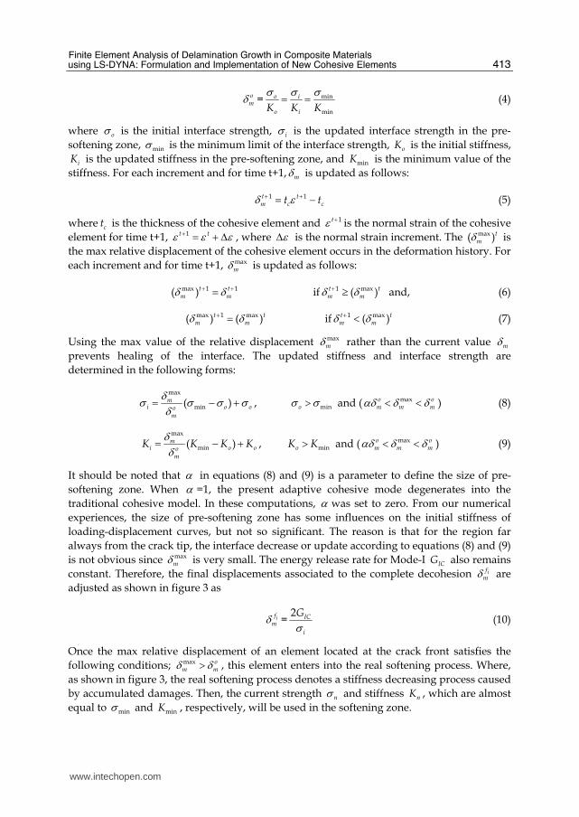
omδ = min
min
o i
o iK K K
σ σ σ= = (4)
where oσ is the initial interface strength, iσ is the updated interface strength in the pre-
softening zone, minσ is the minimum limit of the interface strength, oK is the initial stiffness,
iK is the updated stiffness in the pre-softening zone, and minK is the minimum value of the
stiffness. For each increment and for time t+1, mδ is updated as follows:
1 1t tm c ct tδ ε+ += − (5)
where ct is the thickness of the cohesive element and 1tε + is the normal strain of the cohesive
element for time t+1, 1t tε ε ε+ = + Δ , where εΔ is the normal strain increment. The max( )tmδ is
the max relative displacement of the cohesive element occurs in the deformation history. For
each increment and for time t+1, maxmδ is updated as follows:
max 1 1( )t tm mδ δ+ += if 1 max( )t t
m mδ δ+ ≥ and, (6)
max 1 max( ) ( )t tm mδ δ+ = if 1 max( )t t
m mδ δ+ < (7)
Using the max value of the relative displacement maxmδ rather than the current value mδ
prevents healing of the interface. The updated stiffness and interface strength are
determined in the following forms:
max
min( )mi o oo
m
δσ σ σ σδ= − + , minoσ σ> and ( maxo om m mαδ δ δ< < ) (8)
max
min( )mi o oo
m
K K K Kδδ= − + , minoK K> and ( maxo o
m m mαδ δ δ< < ) (9)
It should be noted that α in equations (8) and (9) is a parameter to define the size of pre-
softening zone. When α =1, the present adaptive cohesive mode degenerates into the
traditional cohesive model. In these computations, α was set to zero. From our numerical
experiences, the size of pre-softening zone has some influences on the initial stiffness of
loading-displacement curves, but not so significant. The reason is that for the region far
always from the crack tip, the interface decrease or update according to equations (8) and (9)
is not obvious since maxmδ is very small. The energy release rate for Mode-I ICG also remains
constant. Therefore, the final displacements associated to the complete decohesion ifmδ are
adjusted as shown in figure 3 as
ifmδ =
2 IC
i
G
σ (10)
Once the max relative displacement of an element located at the crack front satisfies the
following conditions; max om mδ δ> , this element enters into the real softening process. Where,
as shown in figure 3, the real softening process denotes a stiffness decreasing process caused
by accumulated damages. Then, the current strength nσ and stiffness nK , which are almost
equal to minσ and minK , respectively, will be used in the softening zone.
www.intechopen.com
Advances in Composites Materials - Ecodesign and Analysis
414
2. In softening zone, max fom m mδ δ δ≤ < , the constitutive equation is given by
(1 )( ) mm m o
m
dδσ σ ηδ δ= − + $ (11)
where d is the damage variable and can be defined as
max
max
( )
( )
f om m m
f om m m
dδ δ δδ δ δ
−= − , [ ]0,1d∈ (12)
The above adaptive cohesive mode is of the engineering meaning when using coarse meshes
for complex composite structures, which is, in fact, an ‘artificial’ means for achieving the
stable numerical simulation process. A reasonable explanation is that all numerical
techniques are artificial, whose accuracy strongly depends on their mesh sizes, especially at
the front of crack tip. To remove the factitious errors in the simulation results caused by the
coarse mesh sizes in the numerical techniques, some material properties are artificially
adjusted in order to partially alleviate or remove the numerical errors. Otherwise, very fine
meshes need to be used, which may be computationally impractical for very complex
problems from the capabilities of most current computers. Of course, the modified material
parameters should be those which do not have the dominant influences on the physical
phenomena. For example, the interface strength usually controls the initiation of interface
cracks. However, it is not crucial for determining the crack propagation process and final
crack size from the viewpoint of fracture mechanics. Moreover, there has been almost no
clear rule to exactly determine the interface stiffness, which is a parameter determined with
a high degree of freedom in practical cases. Therefore, the effect of the modifications of
interface strength and stiffness can be very small since the practically used onset
displacement omδ for delamination initiation is remained constant in our model. For the
parameters, which dominate the fracture phenomena, should be unchanged. For instance, in
our model, the fracture toughness dominating the behaviors of interface damages is kept
constant.
3. Information finite element implementation
The proposed cohesive element is implemented in LS-DYNA finite element code as a user
defined material (UMAT) using the standard library 8-node solid brick element and *MAT_
USER_ DEFINED_ MATERIAL_MODELS. The keyword input has to be used for the user
interface with data. The following cards are used (LSDYNA User’s Manual; LSTC, 2005) as
shown in table 1.
This approach for the implementation requires modelling the resin rich layer as a non-zero
thickness medium. In fact, this layer has a finite thickness and the volume associated with
the cohesive element can in fact set to be very small by using a very small thickness (e.g. 0.01
mm). To verify these procedures, the crack growth along the interface of a double cantilever
beam (DCB) is studied. The two arms are modelled using standard LS-DYNA 8-node solid
brick elements and the interface elements are developed in a FORTRAN subroutine using
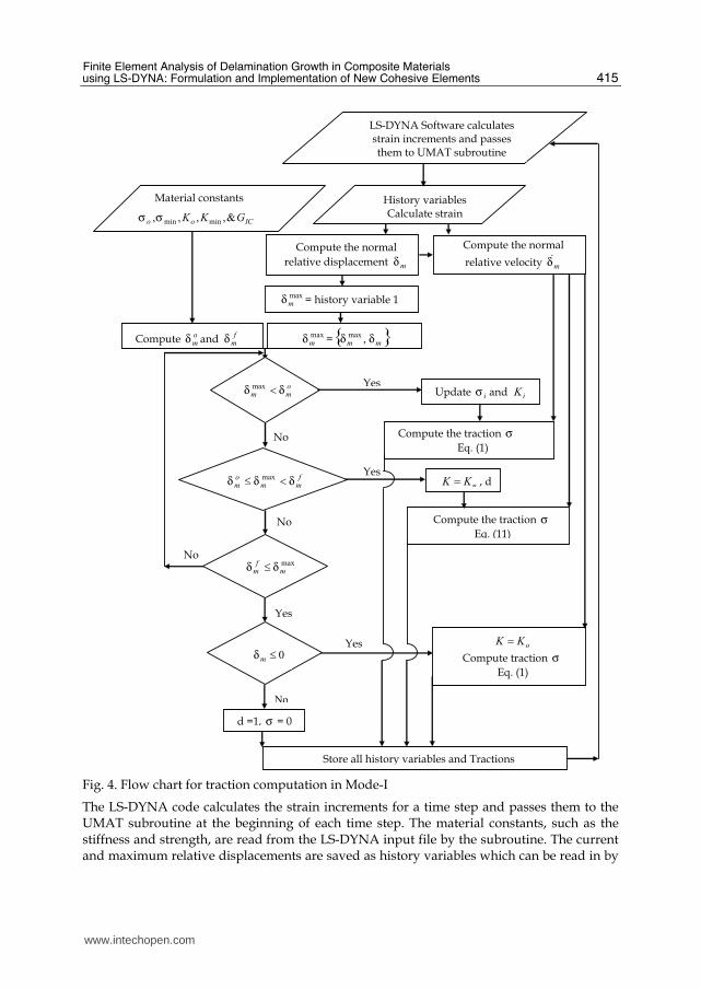
the algorithm shown in figure 4.
www.intechopen.com
Finite Element Analysis of Delamination Growth in Composite Materials using LS-DYNA: Formulation and Implementation of New Cohesive Elements
415
Update iσ and iK
Compute the traction σ
Eq. (1)
Store all history variables and Tractions
Material constants
ICoo GKK &,,,, minminσσ
Compute omδ and f
mδ
Compute the normal
relative displacement mδ
History variables Calculate strain
maxmδ = history variable 1
maxmδ = { }mm δδ ,
max
No
Yesomm δδ <max
No
Yes fmm
om δδδ <≤ max
nKK = , d
Compute the traction σ
Eq. (11)
No maxm
fm δδ ≤
d =1, σ = 0
Yes
No
oKK =
Compute traction σ
Eq. (1)
Yes 0≤mδ
Compute the normal
relative velocity mδɺ
LS-DYNA Software calculates strain increments and passes them to UMAT subroutine
Fig. 4. Flow chart for traction computation in Mode-I
The LS-DYNA code calculates the strain increments for a time step and passes them to the UMAT subroutine at the beginning of each time step. The material constants, such as the stiffness and strength, are read from the LS-DYNA input file by the subroutine. The current and maximum relative displacements are saved as history variables which can be read in by
www.intechopen.com
Advances in Composites Materials - Ecodesign and Analysis
416
the subroutine. Using the history variables, material constants, and strain increments, the subroutine is able to calculate the stresses at the end of the time step by using the constitutive equations. The subroutine then updates and saves the history variables for use in the next time step and outputs the calculated stresses. Note that the *DATABASE _ EXTENT _ BINARY command is required to specify the storage of history variables in the output file.
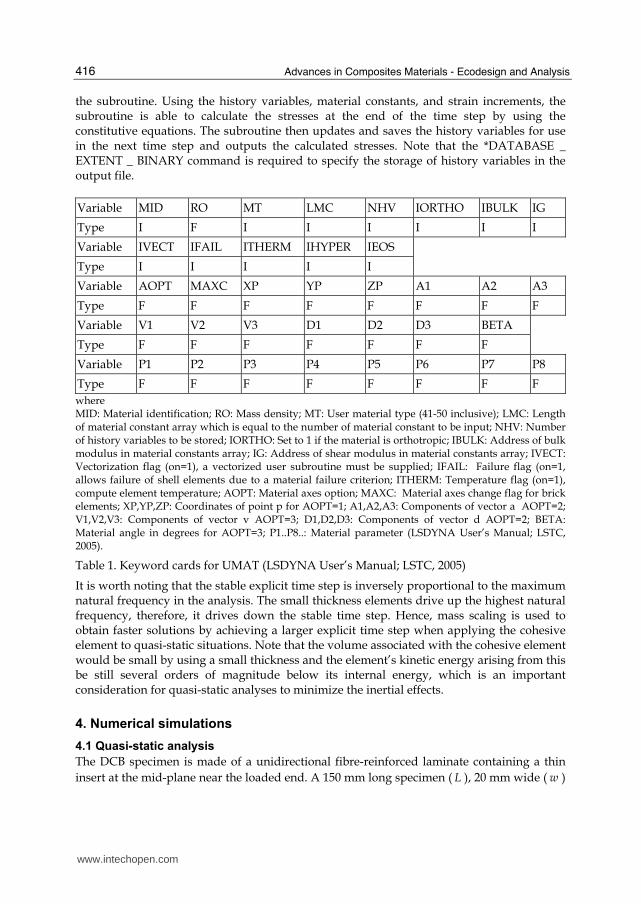
Variable MID RO MT LMC NHV IORTHO IBULK IG
Type I F I I I I I I
Variable IVECT IFAIL ITHERM IHYPER IEOS
Type I I I I I
Variable AOPT MAXC XP YP ZP A1 A2 A3
Type F F F F F F F F
Variable V1 V2 V3 D1 D2 D3 BETA
Type F F F F F F F
Variable P1 P2 P3 P4 P5 P6 P7 P8
Type F F F F F F F F
where MID: Material identification; RO: Mass density; MT: User material type (41-50 inclusive); LMC: Length of material constant array which is equal to the number of material constant to be input; NHV: Number of history variables to be stored; IORTHO: Set to 1 if the material is orthotropic; IBULK: Address of bulk modulus in material constants array; IG: Address of shear modulus in material constants array; IVECT: Vectorization flag (on=1), a vectorized user subroutine must be supplied; IFAIL: Failure flag (on=1, allows failure of shell elements due to a material failure criterion; ITHERM: Temperature flag (on=1), compute element temperature; AOPT: Material axes option; MAXC: Material axes change flag for brick elements; XP,YP,ZP: Coordinates of point p for AOPT=1; A1,A2,A3: Components of vector a AOPT=2; V1,V2,V3: Components of vector v AOPT=3; D1,D2,D3: Components of vector d AOPT=2; BETA: Material angle in degrees for AOPT=3; P1..P8..: Material parameter (LSDYNA User’s Manual; LSTC, 2005).
Table 1. Keyword cards for UMAT (LSDYNA User’s Manual; LSTC, 2005)
It is worth noting that the stable explicit time step is inversely proportional to the maximum natural frequency in the analysis. The small thickness elements drive up the highest natural frequency, therefore, it drives down the stable time step. Hence, mass scaling is used to obtain faster solutions by achieving a larger explicit time step when applying the cohesive element to quasi-static situations. Note that the volume associated with the cohesive element would be small by using a small thickness and the element’s kinetic energy arising from this be still several orders of magnitude below its internal energy, which is an important consideration for quasi-static analyses to minimize the inertial effects.
4. Numerical simulations
4.1 Quasi-static analysis
The DCB specimen is made of a unidirectional fibre-reinforced laminate containing a thin
insert at the mid-plane near the loaded end. A 150 mm long specimen ( L ), 20 mm wide ( w )
www.intechopen.com
Finite Element Analysis of Delamination Growth in Composite Materials using LS-DYNA: Formulation and Implementation of New Cohesive Elements
417
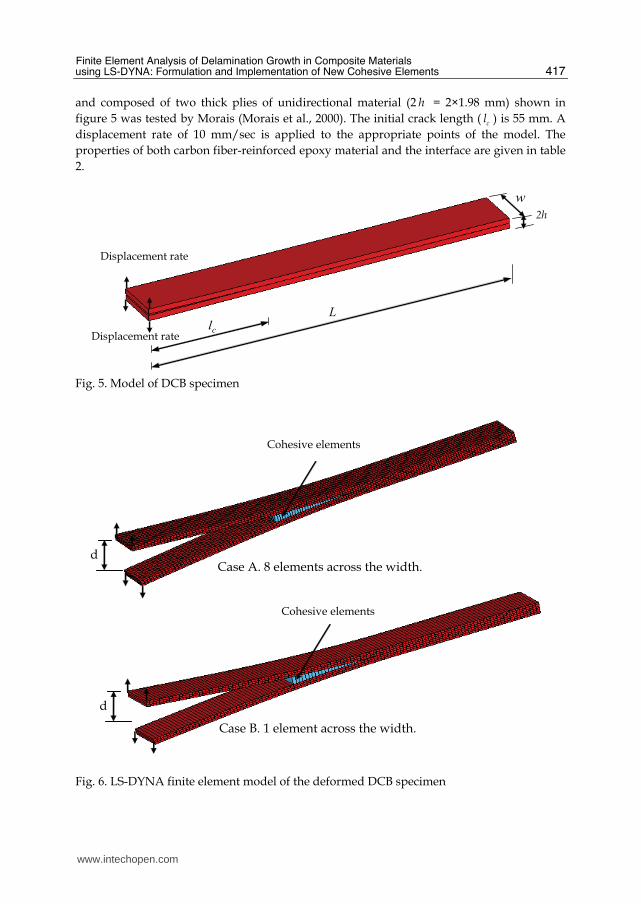
and composed of two thick plies of unidirectional material (2 h = 2×1.98 mm) shown in
figure 5 was tested by Morais (Morais et al., 2000). The initial crack length ( cl ) is 55 mm. A
displacement rate of 10 mm/sec is applied to the appropriate points of the model. The
properties of both carbon fiber-reinforced epoxy material and the interface are given in table
2.
Displacement rate
Displacement rate
L cl
2h
w
Fig. 5. Model of DCB specimen
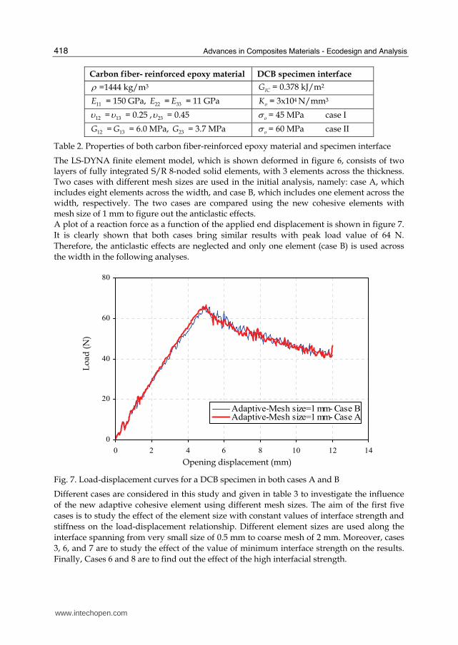
d
Cohesive elements
Case B. 1 element across the width.
d
Cohesive elements
Case A. 8 elements across the width.
Fig. 6. LS-DYNA finite element model of the deformed DCB specimen
www.intechopen.com
Advances in Composites Materials - Ecodesign and Analysis
418
Carbon fiber- reinforced epoxy material DCB specimen interface
ρ =1444 kg/m3 ICG = 0.378 kJ/m2
11E = 150 GPa, 22E = 33E = 11 GPa oK = 3x10⁴ N/mm3
12υ = 13υ = 0.25 , 23υ = 0.45 oσ = 45 MPa case I
12G = 13G = 6.0 MPa, 23G = 3.7 MPa oσ = 60 MPa case II
Table 2. Properties of both carbon fiber-reinforced epoxy material and specimen interface
The LS-DYNA finite element model, which is shown deformed in figure 6, consists of two layers of fully integrated S/R 8-noded solid elements, with 3 elements across the thickness. Two cases with different mesh sizes are used in the initial analysis, namely: case A, which includes eight elements across the width, and case B, which includes one element across the width, respectively. The two cases are compared using the new cohesive elements with mesh size of 1 mm to figure out the anticlastic effects. A plot of a reaction force as a function of the applied end displacement is shown in figure 7.
It is clearly shown that both cases bring similar results with peak load value of 64 N.
Therefore, the anticlastic effects are neglected and only one element (case B) is used across
the width in the following analyses.
Fig. 7. Load-displacement curves for a DCB specimen in both cases A and B
Different cases are considered in this study and given in table 3 to investigate the influence
of the new adaptive cohesive element using different mesh sizes. The aim of the first five
cases is to study the effect of the element size with constant values of interface strength and
stiffness on the load-displacement relationship. Different element sizes are used along the
interface spanning from very small size of 0.5 mm to coarse mesh of 2 mm. Moreover, cases
3, 6, and 7 are to study the effect of the value of minimum interface strength on the results.
Finally, Cases 6 and 8 are to find out the effect of the high interfacial strength.
0
20
40
60
80
0 2 4 6 8 10 12 14
Adaptive-Mesh size=1 mm- Case BAdaptive-Mesh size=1 mm- Case A
Opening displacement (mm)
Lo
ad (
N)
www.intechopen.com
Finite Element Analysis of Delamination Growth in Composite Materials using LS-DYNA: Formulation and Implementation of New Cohesive Elements
419
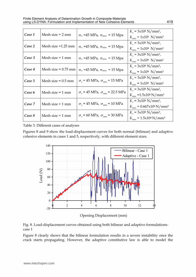
Case 1 Mesh size = 2 mm oσ =45 MPa, minσ = 15 Mpa oK = 3x10⁴ N/mm3,
minK = 1x10⁴ N/mm3
Case 2 Mesh size =1.25 mm oσ =45 MPa, minσ = 15 Mpa oK = 3x10⁴ N/mm3,
minK = 1x10⁴ N/mm3
Case 3 Mesh size = 1 mm oσ =45 MPa, minσ = 15 Mpa oK = 3x10⁴ N/mm3,
minK = 1x10⁴ N/mm3
Case 4 Mesh size = 0.75 mm oσ =45 MPa, minσ = 15 Mpa oK = 3x10⁴ N/mm3,
minK = 1x10⁴ N/mm3
Case 5 Mesh size = 0.5 mm oσ = 45 MPa, minσ = 15 MPa oK = 3x10⁴ N/mm3,
minK = 1x10⁴ N/mm3
Case 6 Mesh size = 1 mm oσ = 45 MPa, minσ = 22.5 MPaoK = 3x10⁴ N/mm3,
minK =1.5x10⁴ N/mm3
Case 7 Mesh size = 1 mm oσ = 45 MPa, minσ = 10 MPa oK = 3x10⁴ N/mm3,
minK = 0.667x10⁴ N/mm3
Case 8 Mesh size = 1 mm oσ = 60 MPa, minσ = 30 MPa oK = 3x10⁴ N/mm3,
minK = 1.5x10⁴ N/mm3
Table 3. Different cases of analyses
Figures 8 and 9 show the load-displacement curves for both normal (bilinear) and adaptive
cohesive elements in cases 1 and 5, respectively, with different element sizes.
Fig. 8. Load-displacement curves obtained using both bilinear and adaptive formulations-case 1
Figure 8 clearly shows that the bilinear formulation results in a severe instability once the crack starts propagating. However, the adaptive constitutive law is able to model the
-20
0
20
40
60
80
100
120
140
0 2 4 6 8 10 12 14
Bilinear - Case 1
Adaptive - Case 1
L
oad
(N
)
Opening Displacement (mm)
www.intechopen.com
Advances in Composites Materials - Ecodesign and Analysis
420
smooth, progressive crack propagation. It is worth mentioning that the bilinear formulation brings smooth results by decreasing the element size. And it is clearly noticeable from figure 9 that both bilinear and adaptive formulations are found to be stable in case 5 with very small element size. This indicates that elements with very small sizes need to be used in the softening zone to obtain high accuracy using bilinear formulation. However, this leads to large computational costs compare to case 1. On the other hand, figure 10, which presents the load-displacement curves, obtained with the use of the adaptive formulation in the first five cases, show a great agreement of the results regardless the mesh size. Adaptive cohesive model (ACM) can yield very good results from the aspects of the peak load and the slope of loading curve if minσ is properly defined. From this figure, it can be found that the different
mesh sizes result in almost the same loading curves. Even, with 2 mm mesh size, which considerable large size, although the oscillation is higher compared with those of fine mesh size, ACM still models the propagation in stable manner. The oscillation of the curve once the crack starts propagates became less by decreasing the mesh size. Therefore, the new adaptive model can be used with considerably larger mesh size and the computational cost will be greatly minimized.
Fig. 9. Load-displacement curves obtained using both bilinear and adaptive formulations-case 5
The load-displacement curves obtained from the numerical simulation of cases 3, 6 and 7 are
presented in figure 11 together with experimental data (Camanho & Davila, 2002). It can be
seen that the average maximum load obtained in the experiments is 62.5 N, whereas the
average maximum load predicted form the three cases is 65 N. It can be observed that
numerical curves slightly overestimate the load. It is worth noting that with the decrease of
interface strength, the result is stable, very good result can be obtained by comparing with
the experimental ones, however, the slope of loading curve before the peak load is obviously
lower than those of experimental ones (case 7; minσ =10.0 MPa). In case 6 ( minσ =22.5 MPa)
and case 3 ( minσ =15 MPa), excellent agreements between the experimental data and the
0
20
40
60
80
0 2 4 6 8 10 12 14
Bilinear - Case 5
Adaptive - Case 5
Lo
ad (
N)
Opening displacement (mm)
www.intechopen.com
Finite Element Analysis of Delamination Growth in Composite Materials using LS-DYNA: Formulation and Implementation of New Cohesive Elements
421
numerical predictions is obtained although the oscillation in case 6 is higher compared with
those of case 3. Also, the slope of loading curve in case 3 is closer to the experimental results
compared with that in case 6.
Fig. 10. Load-displacement curves obtained using the adaptive formulation-cases 1-5
Fig. 11. Comparison of experimental and numerical simulations using the adaptive formulation - cases 3, 6 and 7
0
20
40
60
80
0 2 4 6 8 10 12 14
Adaptive - Case 1Adaptive - Case 2Adaptive - Case 3Adaptive - Case 4Adaptive - Case 5
Opening displacement (mm)
L
oad
(N
)
0
20
40
60
80
0 2 4 6 8 10 12 14
Adaptive - Case 6
Adaptive - Case 3
Adaptive - Case 7
Experiment
L
oad
(N
)
Opening displacement (mm)
www.intechopen.com
Advances in Composites Materials - Ecodesign and Analysis
422
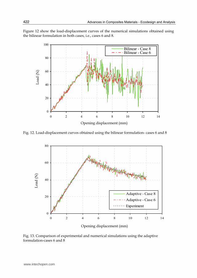
Figure 12 show the load-displacement curves of the numerical simulations obtained using the bilinear formulation in both cases, i.e., cases 6 and 8.
Fig. 12. Load-displacement curves obtained using the bilinear formulation- cases 6 and 8
Fig. 13. Comparison of experimental and numerical simulations using the adaptive formulation-cases 6 and 8
0
20
40
60
80
100
0 2 4 6 8 10 12 14
Bilinear - Case 8Bilinear - Case 6
Opening displacement (mm)
L
oad
(N
)
0
20
40
60
80
0 2 4 6 8 10 12 14
Adaptive - Case 8
Adaptive - Case 6
Experiment
Opening displacement (mm)
L
oad
(N
)
www.intechopen.com
Finite Element Analysis of Delamination Growth in Composite Materials using LS-DYNA: Formulation and Implementation of New Cohesive Elements
423
The bilinear formulations results in a severe instabilities once the crack starts propagation. It is also shown that a higher maximum traction (case 8) resulted in a more severe instability compared to a lower maximum traction (case 6). However, as shown in figure 13, the load-displacement curves of the numerical simulations obtained using the adaptive formulations are very similar in both cases. The maximum load obtained from case 8 is found to be 69 N while in case 6, the maximum load obtained is 66 N. The adaptive formulation is able to model the smooth, progressive crack propagation and also to produce close results compared with the experimental ones.
4.2 Dynamic analysis
The DCB specimen, as shown in figure 5, is made of an isotropic fibre-reinforced laminate
containing a thin insert at the mid-plane near the loaded end, L =250 mm, w =25 mm
and h =1.5 mm, was analyzed by Moshier (Moshier, 2006). The initial crack length ( cl ) is 34
mm. A displacement rate of 650 mm/sec is applied to the appropriate points of the model.
Young’s modulus, density and Poisson’s ratio of carbon fibre-reinforced epoxy material are
given as E =115 GPa, ρ =1566 Kg/m3, and υ =0.27, respectively. The properties of the DCB
specimen interface are given as following: ICG = 0.7 kJ/m2, oK = 1x10⁵ N/mm3, minK =
Similarly, the LS-DYNA finite element model consists of two layers of fully integrated S/R
8-noded solid elements, with 3 elements across the thickness. The adaptive rate-dependent
cohesive zone model is implemented using a user defined cohesive material model in LS-
DYNA. Two different values of viscosity parameter are used in the simulations; η = 0.01
and 1.0 N·sec/mm3, respectively. Note that η is a material parameter depending on
deformation rate, which appears in equations (1) and (11). When η =0, it would be a
traditional model without rate dependence. By observing equation (1), η determines the
ratio between viscosity stress mηδ$ and interface strength mσ since mσ σ= i if equations (1)
and (4) are considered by setting K K= i . For example, if mδ$ = 6.5 mm/sec is assumed on the
interface here (i.e. 1% of loading rate). η = 0.01 N·sec/mm3 corresponds to a low viscosity
stress of 0.065MPa, which is much lower than the initial interface strength of 50 MPa.
However, η =1.0 N·sec/mm3 corresponds to a viscosity stress of 6.5 MPa, which is around
13% of the interface strength, and denotes a higher rate dependence. In addition, two sets of
simulations are performed here. The first set involves simulations of normal (bilinear)
cohesive model. The second set involves simulations of the new adaptive rate-dependent
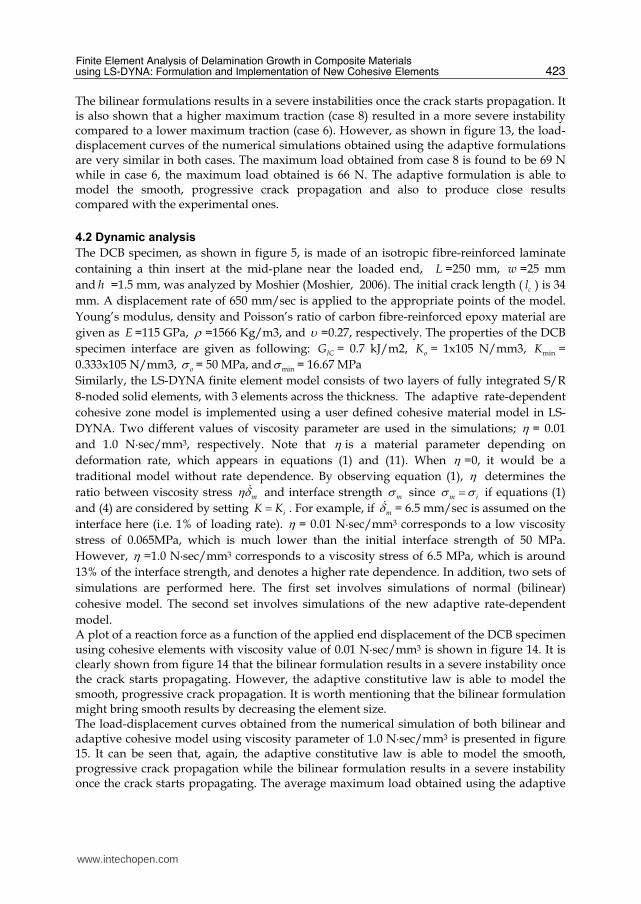
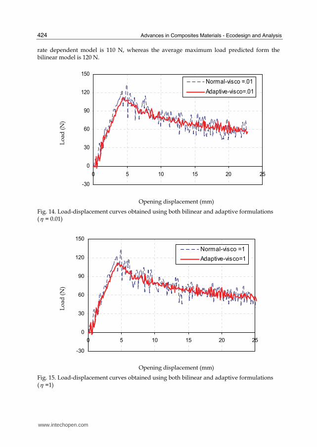
model. A plot of a reaction force as a function of the applied end displacement of the DCB specimen using cohesive elements with viscosity value of 0.01 N·sec/mm3 is shown in figure 14. It is clearly shown from figure 14 that the bilinear formulation results in a severe instability once the crack starts propagating. However, the adaptive constitutive law is able to model the smooth, progressive crack propagation. It is worth mentioning that the bilinear formulation might bring smooth results by decreasing the element size. The load-displacement curves obtained from the numerical simulation of both bilinear and adaptive cohesive model using viscosity parameter of 1.0 N·sec/mm3 is presented in figure 15. It can be seen that, again, the adaptive constitutive law is able to model the smooth, progressive crack propagation while the bilinear formulation results in a severe instability once the crack starts propagating. The average maximum load obtained using the adaptive
www.intechopen.com
Advances in Composites Materials - Ecodesign and Analysis
424
rate dependent model is 110 N, whereas the average maximum load predicted form the bilinear model is 120 N.
Lo
ad (
N)
-30
0
30
60
90
120
150
0 5 10 15 20 25
Normal-visco =.01
Adaptive-visco=.01
Opening displacement (mm)
Fig. 14. Load-displacement curves obtained using both bilinear and adaptive formulations (η = 0.01)
Lo
ad (
N)
-30
0
30
60
90
120
150
0 5 10 15 20 25
Normal-visco =1
Adaptive-visco=1
Opening displacement (mm)
Fig. 15. Load-displacement curves obtained using both bilinear and adaptive formulations (η =1)
www.intechopen.com
Finite Element Analysis of Delamination Growth in Composite Materials using LS-DYNA: Formulation and Implementation of New Cohesive Elements
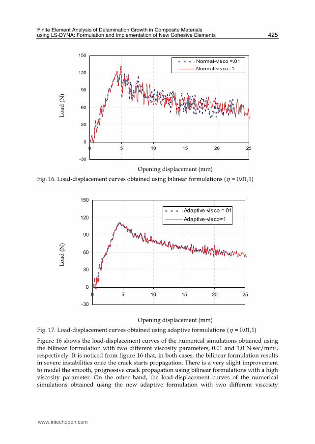
Figure 16 shows the load-displacement curves of the numerical simulations obtained using the bilinear formulation with two different viscosity parameters, 0.01 and 1.0 N·sec/mm3, respectively. It is noticed from figure 16 that, in both cases, the bilinear formulation results in severe instabilities once the crack starts propagation. There is a very slight improvement to model the smooth, progressive crack propagation using bilinear formulations with a high viscosity parameter. On the other hand, the load-displacement curves of the numerical simulations obtained using the new adaptive formulation with two different viscosity
www.intechopen.com
Advances in Composites Materials - Ecodesign and Analysis
426
parameters, 0.01 and 1.0 N·sec/mm3, respectively, is depicted in figure 17. It is clear from figure 17 that the adaptive formulation able to model the smooth, progressive crack propagation irrespective the value of the viscosity parameter. More parametric studies will be performed in the ongoing research to accurately predict the effect of very high value of viscosity parameter on the results using both bilinear and adaptive cohesive element formulations.
5. Conclusions
A new adaptive cohesive element is developed and implemented in LS-DYNA to overcome the numerical insatiability occurred using the bilinear cohesive model. The formulation is fully three dimensional, and can be simulating mixed-mode delamination, however, in this study, only DCB test in Mode-I is used as a reference to validate the numerical simulations. Quasi-static and dynamic analyses are carried out in this research to study the effect of the new constitutive model. Numerical simulations showed that the new model is able to model the smooth, progressive crack propagation. Furthermore, the new model can be effectively used in a range of different element size (reasonably coarse mesh) and can save a large amount of computation. The capability of the new mode is proved by the great agreement obtained between the numerical simulations and the experimental results.
6. Acknowledgement
The author wishes to acknowledge the research support and constitutive models provided for this ongoing research by Professor Ning Hu.
7. References
Camanho, P. & Davila, C. (2004). Fracture analysis of composite co-cured structural joints using decohesion elements. Journal of Fatigue & Fracture of Engineering Materials & Structures, Vol. 27, 745-757
Camanho, P.; Da´vila, C. & De Moura, M. (2003). Numerical simulation of mixed-mode progressive delamination in composite materials. Journal of Composite Materials, Vol. 37, No. 16, 1415-38
Camanho, P. & Davila C. (2002). Mixed-mode decohesion finite elements for the simulation of delamination in composite materials. NASA/TM-2002-211737, 1-37
Camanho, P.; Davila, C. & Ambur, D. (2001). Numerical simulation of delamination growth in composite materials. NASA-TP-211041, 1-19
Chen, J.; Crisfield, M.; Kinloch, A.; Busso, E.; Matthews, F. & Qiu, Y. (1999). Predicting progressive delamination of composite material specimens via interface elements. Mechanics of Composite Material and structures, Vol. 6, No. 4, 301-317
Costanzo, F. & Walton, J. (1997). A study of dynamic crack growth in elastic materials using a cohesive zone model. International Journal of Engineering Science, Vol. 35, No. 12/13, 1085-1114
Cui, W. & Wisnom, M. (1993). A combined stress-based and fracture mechanics-based model for predicting delamination in composites. Composites, Vol. 24, 467-474
www.intechopen.com
Finite Element Analysis of Delamination Growth in Composite Materials using LS-DYNA: Formulation and Implementation of New Cohesive Elements
427
Davila, C.; Camanho, P. & De Moura M. (2001). Mixed-mode decohesion elements for analyses of progressive delamination. 42nd AIAA/ASME/ASCE/AHS/ASC Structures, Structural Dynamics and Material Conference, pp. 1-12, April 2001, Washington, USA
De Moura, M.; Gonçalves, J.; Marques, A. & De Castro, P. (2000). Prediction of compressive strength of carbon-epoxy laminates containing delaminations by using a mixed-mode damage model. Composite Structure, Vol. 50, No. 2, 151–157
De Moura, M.; Goncalves, J.; Marques, A. & De Castro, P. (1997). Modeling compression failure after low velocity impact on laminated composites using interface elements. Journal of Composite Materials, Vol. 31, No. 15, 1462-1479
De Xie, A. & Waas, A. (2006). Discrete cohesive zone model for mixed-mode fracture using finite element analysis. Engineering Fracture Mechanics, Vol. 73, No. 13, 1783-1796
Gao, Y. & Bower, A. (2004). A simple technique for avoiding convergence problems in finite element simulations of crack nucleation and growth on cohesive interfaces. Modelling and Simulation in Materials Science and Engineering, Vol. 12, No. 3, 453-463
Glennie, E. (1971). A strain-rate dependent crack model. Journal of the Mechanics and Physics of Solids, Vol. 19, No. 5, 255-272
Goncalves, J.; De Moura, M.; De Castro, P. & Marques, A. (2000). Interface element including point-to-surface constraints for three-dimensional problems with damage propagation. Engineering Computations, Vol. 17, No. 1, 28-47
Gustafson, P. & Waas, A. (2008). Efficient and robust traction laws for the modeling of adhesively bonded joints. 49th AIAA/ASME/ASCE/AHS/ASC Structures, Structural Dynamics, and Materials Conference, pp. 1-16, April 2008, Schaumburg, IL, USA
Hu, N.; Zemba, Y.; Okabe, T.; Yan, C.; Fukunaga, H. & Elmarakbi, A. (2008). A new cohesive model for simulating delamination propagation in composite laminates under transverse loads. Mechanics of Materials, Vol. 40, No. 11, 920-935
Hu, N.; Zemba, Y.; Fukunaga, H.; Wang, H. & Elmarakbi, A. (2007). Stable numerical simulations of propagations of complex damages in composite structures under transverse loads. Composite Science and Technology, Vol. 67, No. 3-4, 752-765
Kubair, D.; Geubelle, P. & Huang, Y. (2003). Analysis of a rate dependent cohesive model for dynamic crack propagation. Engineering Fracture Mechanics, Vol. 70, No. 5, 685-704
LSTC, Livermore Software Technology Corporation, California, USA, LS-DYNA 970, 2005 Mi, Y.; Crisfield, M. & Davis, G. (1998). Progressive delamination using interface element.
Journal of Composite Materials, Vol. 32, No. 14, 1246-1272 Morais, A.; Marques, A. & De Castro, P. (2000). Estudo da aplicacao de ensaios de fractura
interlaminar de mode I a laminados compositos multidireccionais. Proceedings of the 7as jornadas de fractura, Sociedade Portuguesa de Materiais, p. 90-95, 2000, Portugal
Moshier, M. (2006). Ram load simulation of wing skin-spar joints: new rate-dependent cohesive model. RHAMM Technologies LLC, USA, Report No. R-05-01
Petrossian, Z. & Wisnom, M. (1998). Prediction of delamination initiation and growth from discontinues plies using interface elements. Composite A, Vol. 29, 503-515
Pinho, S.; Iannucci, L. & Robinson, P. (2006). Formulation and implementation of decohesion elements in an explicit finite element code. Composite A, Vol. 37, 778-789
Pinho, S.; Camanho, P. & De Moura, M. (2004). Numerical simulation of the crushing process of composite materials. International Journal of Crashworthiness, Vol. 9, No. 3, 263–76
www.intechopen.com
Advances in Composites Materials - Ecodesign and Analysis
428
Reddy, E.; Mello, F. & Guess, T. (1997). Modeling the initiation and growth of delaminations in composite structures. Journal of Composite Materials, Vo. 31, No. 8, 812-831
Riks, E. (1979). An incremental approach to the solution of snapping and buckling problems. International Journal of Solid and Structures, Vo. 15, 529-551
Shahwan, K. & Waas, A. (1997). Non-self-similar decohesion along a finite interface of unilaterally constrained delaminations. Proceeding of the Royal Society of London A, Vol. 453, No. 1958, 515-550
Tvergaard, V. & Hutchinson, J. (1996). Effect of strain-dependent cohesive zone model on predictions of crack growth resistance. International Journal of Solid and Structures, Vol. 33, No. 20-22, 3297-3308
Xu, D.; Hui, E.; Kramer, E. & Creton, C. (1991). A micromechanical model of crack growth along polymer interfaces. Mechanics of Materials, Vol. 11, No. 3, 257-268
www.intechopen.com
Advances in Composite Materials - Ecodesign and AnalysisEdited by Dr. Brahim Attaf
ISBN 978-953-307-150-3Hard cover, 642 pagesPublisher InTechPublished online 16, March, 2011Published in print edition March, 2011
InTech ChinaUnit 405, Office Block, Hotel Equatorial Shanghai No.65, Yan An Road (West), Shanghai, 200040, China
Phone: +86-21-62489820 Fax: +86-21-62489821
By adopting the principles of sustainable design and cleaner production, this important book opens a newchallenge in the world of composite materials and explores the achieved advancements of specialists in theirrespective areas of research and innovation. Contributions coming from both spaces of academia and industrywere so diversified that the 28 chapters composing the book have been grouped into the following main parts:sustainable materials and ecodesign aspects, composite materials and curing processes, modelling andtesting, strength of adhesive joints, characterization and thermal behaviour, all of which provides an invaluableoverview of this fascinating subject area. Results achieved from theoretical, numerical and experimentalinvestigations can help designers, manufacturers and suppliers involved with high-tech composite materials toboost competitiveness and innovation productivity.
How to referenceIn order to correctly reference this scholarly work, feel free to copy and paste the following:
Ahmed Elmarakbi (2011). Finite Element Analysis of Delamination Growth in Composite Materials using LS-DYNA: Formulation and Implementation of New Cohesive Elements, Advances in Composite Materials -Ecodesign and Analysis, Dr. Brahim Attaf (Ed.), ISBN: 978-953-307-150-3, InTech, Available from:http://www.intechopen.com/books/advances-in-composite-materials-ecodesign-and-analysis/finite-element-analysis-of-delamination-growth-in-composite-materials-using-ls-dyna-formulation-and-