FINITE ELEMENT ANALYSIS OF SOME SOIL-STRUCTURE ' INTERACTION PROBLEMS; by Ahmad Ra i f,, A 1 ame dd i ne,, Thesis submitted to the Graduate Faculty of the Virginia Polytechnic Institute and State University in partial fulfillment of the requirement of the degree of MASTER OF SCIENCE in Civil Engineering APPROVED: C. S. Desai, • S. Sture T. KuppusarnY March, 1979 Blacksburg, Virginia
Transcript
FINITE ELEMENT ANALYSIS OF SOME SOIL-STRUCTURE '
INTERACTION PROBLEMS;
by
Ahmad Ra i f,, A 1 ame dd i ne,,
Thesis submitted to the Graduate Faculty of the
Virginia Polytechnic Institute and State University
in partial fulfillment of the requirement of the degree of
MASTER OF SCIENCE
in
Civil Engineering
APPROVED:
C. S. Desai, Cha1rma~ •
S. Sture T. KuppusarnY
March, 1979
Blacksburg, Virginia
ACKNOWLEDGEMENTS
The author would like to express his thanks to his advisor,
for his encouragement and assistance in identifying
the problems and continued help towards the development of this
thesis. Special thanks to for his unbounded help
and inexhaustible patience inl>Ssistance for various aspects of the
study. Thanks also to for his advice and criticism.
Above all I am grateful for my family for assistance, both
moral and financial, for providing love, encouragement and hope
without which I would have surely failed in this endeavor.
ii
ACKNOWLEDGEMENTS
LIST OF FIGURES
LIST OF TABLES
NOMENCLATURE
I INTRODUCTION •
TABLE OF CONTENTS
II SOIL-STRUCTURE INTERACTION
Page
. ii
. iii
. vii
viii
1
3
2.1 Introduction 3
2.2 Coefficient of Subgrade Reaction 4
2.3 Resistance-Deflection Curves 4
2.4 Beams on Elastic Foundations 8
2.5 Laterally Loaded Piles . 10
2.6 Plates on Elastic Foundations . 11
2. 7 Pi le Group . 13
III THE FINITE ELEMENT MODEL . . 17
3.1 Introduction . 17
3.2 Beam-Column Element • • 17
3.3 Plate Bending Element . 22
3.4 System Assembly, Addition of Constraints and Method of Solution . 37
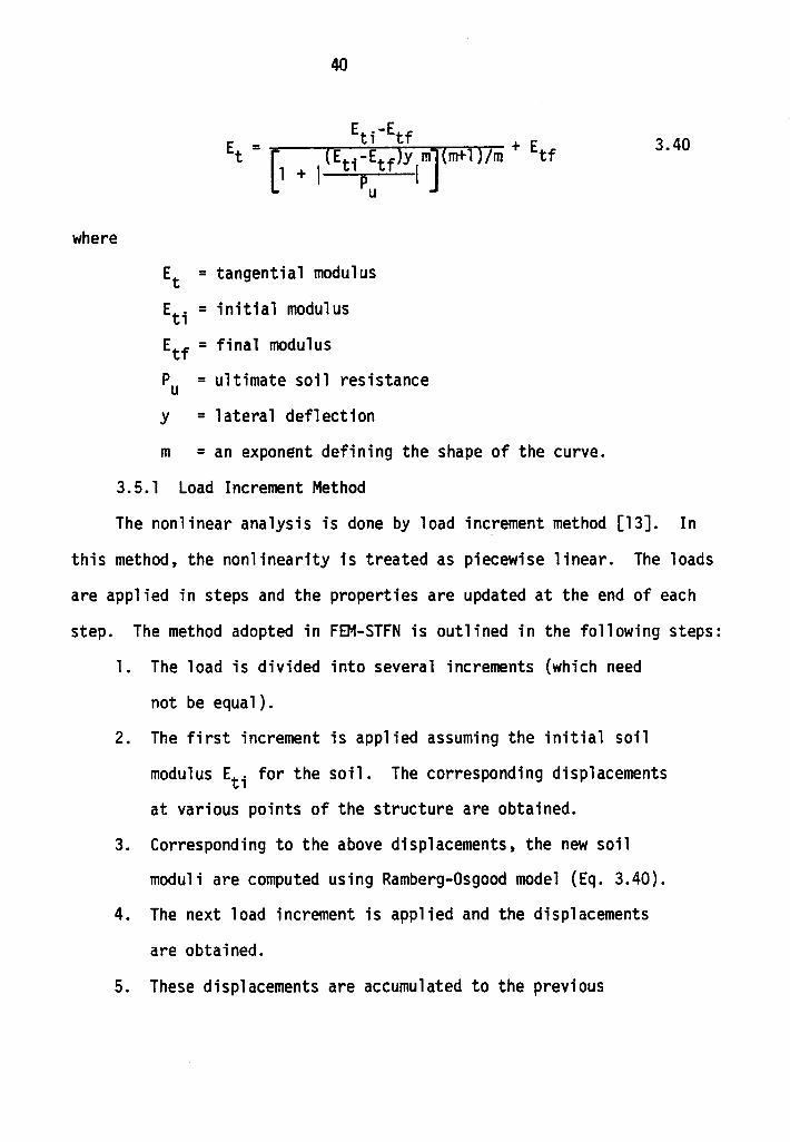
3.5 Simulation of Soil Behavior . • 39
3.5.1 Load Increment Method . 40
3.6 Stress Transfer . . 42
iii
iv
IV APPLICATIONS 45
4 .1 Cantilever Beam on Elastic Foundation 45
4.2 Solution by Finite Element Method and Photoelastic Study of a Beam on Elastic Foundation . 47
4.3 Deep Beam on Elastic Foundation 52
4.4 Convergence of Deflection and Moments 1 n a Simply
Supported Plate Subjected to a uniform Load 54
4.5 Square Plate on Elastic Foundation Subjected to Column Loads 59
4.6 Mat Foundation with a Frame 59
4.7 Pi 1 e Group Mode 1 65
4. 7 .1 Parametric Study 78
4.7.la Effect of Variation of Initial Soil Modulus 79
4.7.lb Effect of Variation of Modulus of Elasticity of the Piles 79
4.7.lc Effect of Variation of Modulus of Elasticity of the Plate 82
v POSSIBLE EXTENSIONS 84
VI CONCLUSIONS . 85
REFERENCES 86
VITA . 90
Figure
2. 1
2.2
3. 1
3.2
3.3
3.4
3.5
4.1
4.2
LIST OF FIGURES
Graphical Representation of p-y Curves
Graphical Representation of Et Increasing with Depth . . . . .
General Beam-Column Element .
Plate Element in Local and Global Coordinates
Flat Rectangular Plate Element
The Ramberg-Osgood Model
Graphical Representation of Stress Transfer Technique
Cantilever Beam on Elastic Foundation
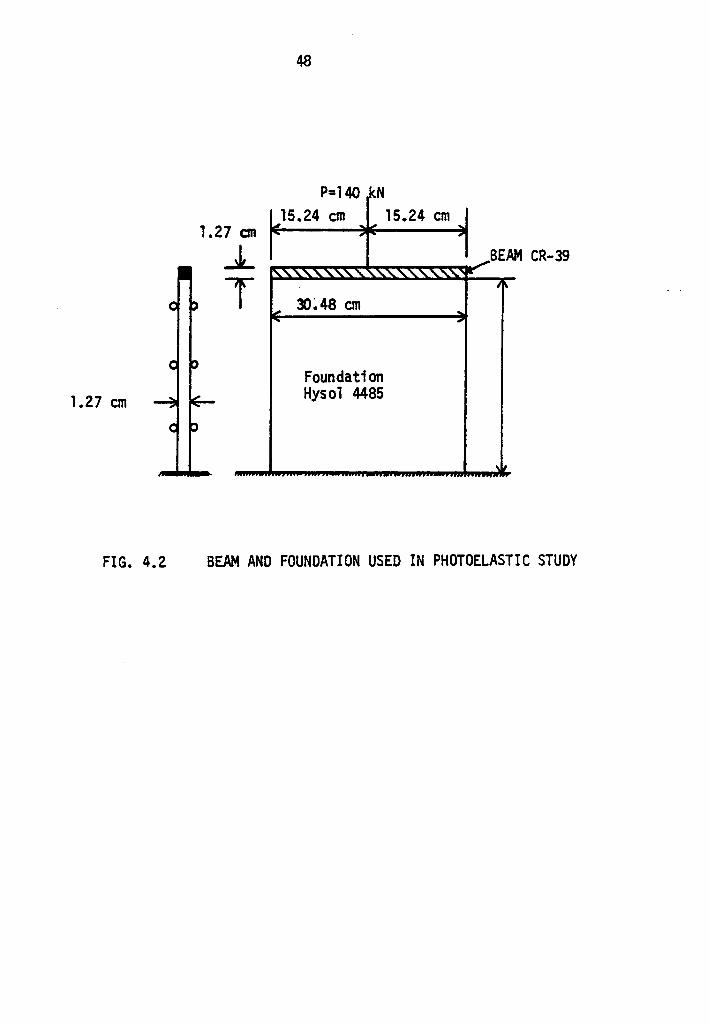
Beam and Foundation Used in Photoelastic Study
Page
6
7
18
24
25
41
44
46
48
4.3 Contact Pressure under Beam Supported on Elastic
Foundation and Subjected to a Concentrated Load . 50
4.4 Bending Moment in a Beam Supported on Elastic Foundation and Subjected to a Concentrated Load 51
4.5 Deflected Shape of a Beam Supported on Elastic Foundation and Subjected to a Concentrated Load Before and After Stress Transfer 53
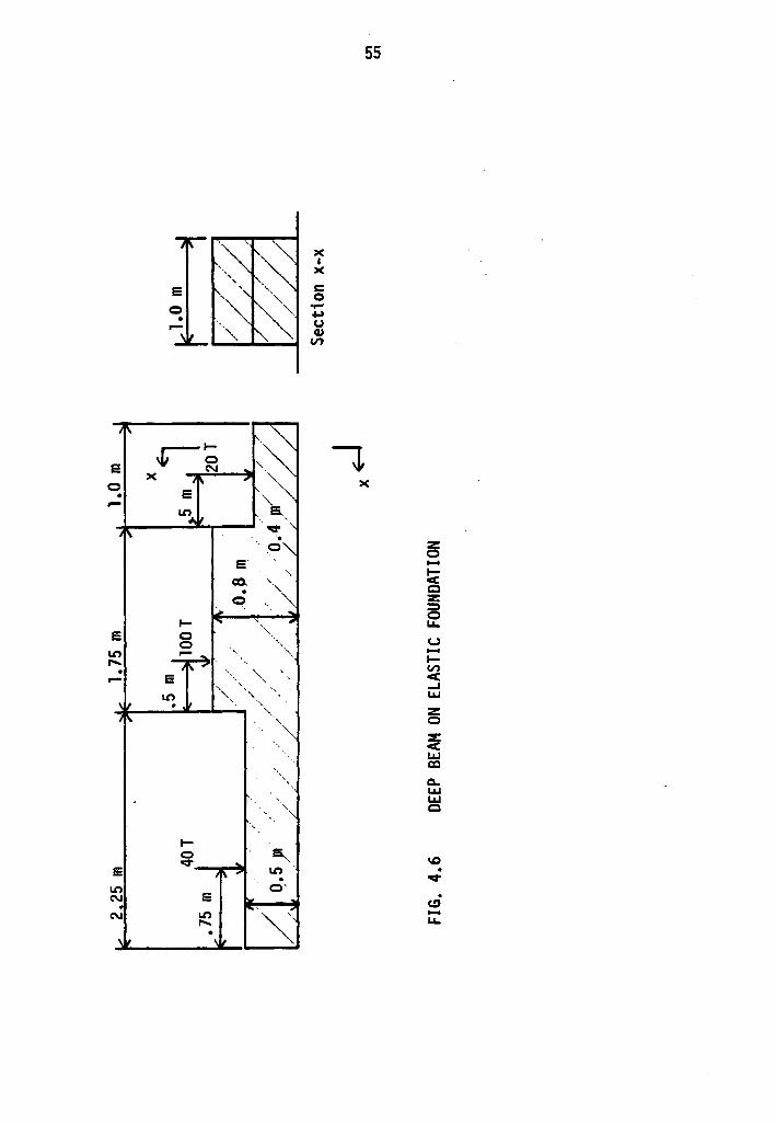
4.6 Deep Beam on Elastic Foundation 55
4.7 Contact Pressure under Deep Beam on Elastic Foundation 56
4.8 Convergence of Central Deflection and Central Moment in a Uniformly Loaded Simply Supported Plate 58
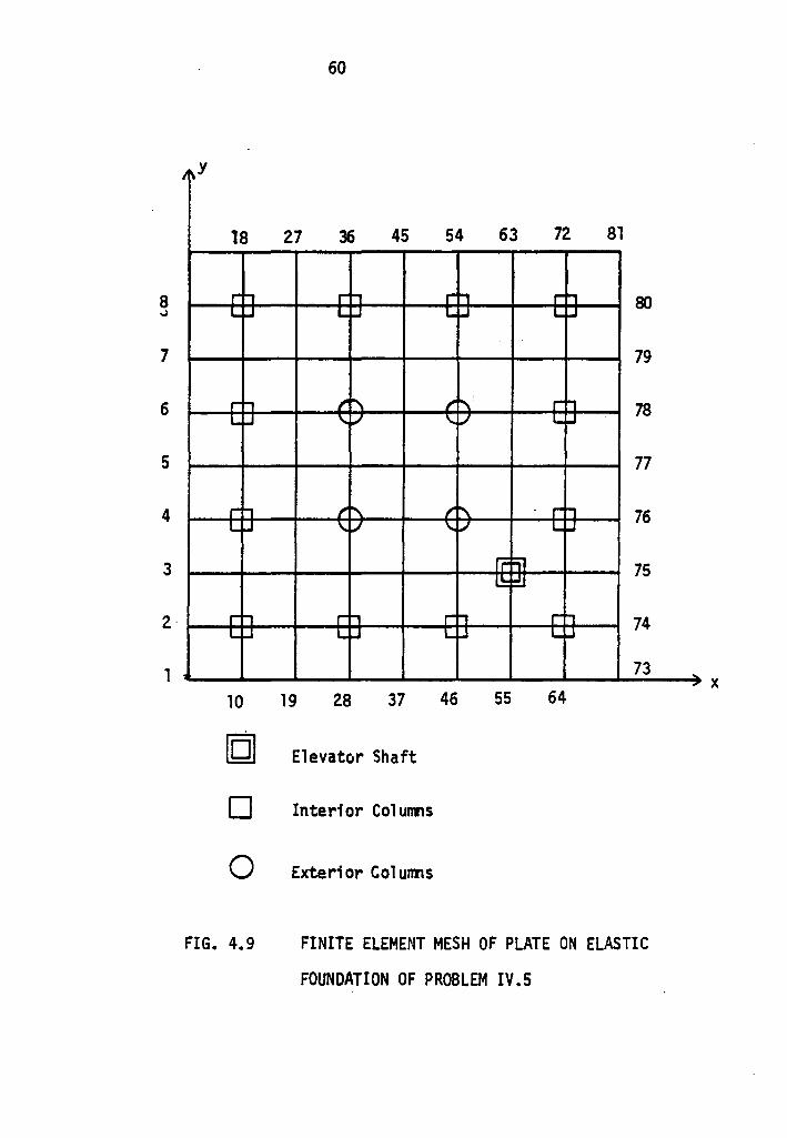
4.9 Finite Element Mesh of Plate on Elastic Foundation of Problem IV.5 . 60
v
4.10
4.11
4.12
4.13
4.14
4.15
4.16
4. 17
4.18
4.19
4.20
vi
Deflections Along Line 64-72 for Plate on Elastic Foundation (Problem IV.5} •
Dimensions and Loading on Plate and Frame {Problem IV.6)
Finite Element Mesh Used in Problem IV.6 (Frame and Plate) •
Contact Pressure Along Line 9-19 for Problem IV.6
Pi le Group Model
p-y Curves for Sand (Problem IV.7)
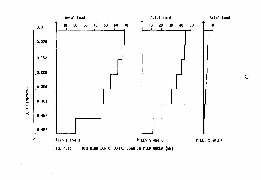
Distribution of Axial Load in Pile Group •
Distribution of f'oments along Piles
Distribution of f'oment Along Typical Sections of Pile Cap •
Deflected Shape of Pile Group {Deflections are Highly Exaggerated
Lateral Load vs. Deflection
61
62
64
66
67
69
73
74
75
76
77
LIST OF TABLES
Table Page
2 .1 Values of Coefficient of Subgrade Reaction Es 5
3. 1 Membrane Stiffness Matrix 31
3.2 Membrane Load Vector • 32
3.3 Bending Load Vector . 34
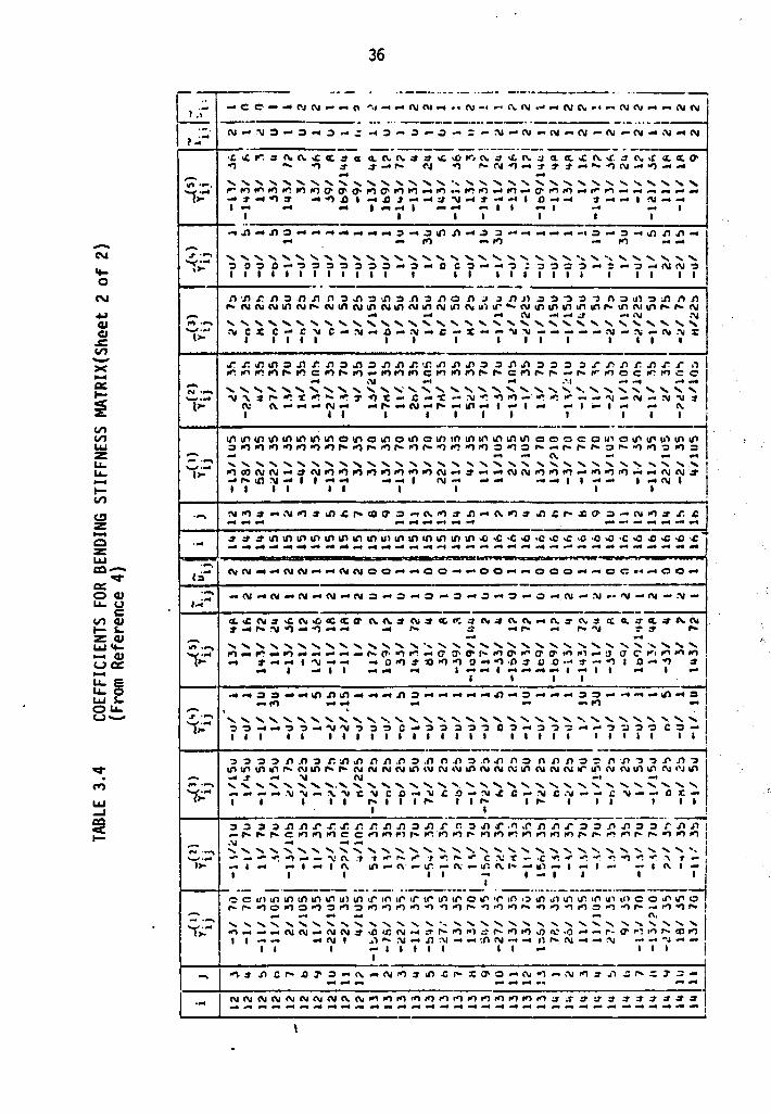
3.4 Coefficients for Bending Stiffness Matrix 35
4.1 Parameters for Ramberg-Osgood Model 70
4.2 Comparison of Axial Load Distribution in the Pile Group 72
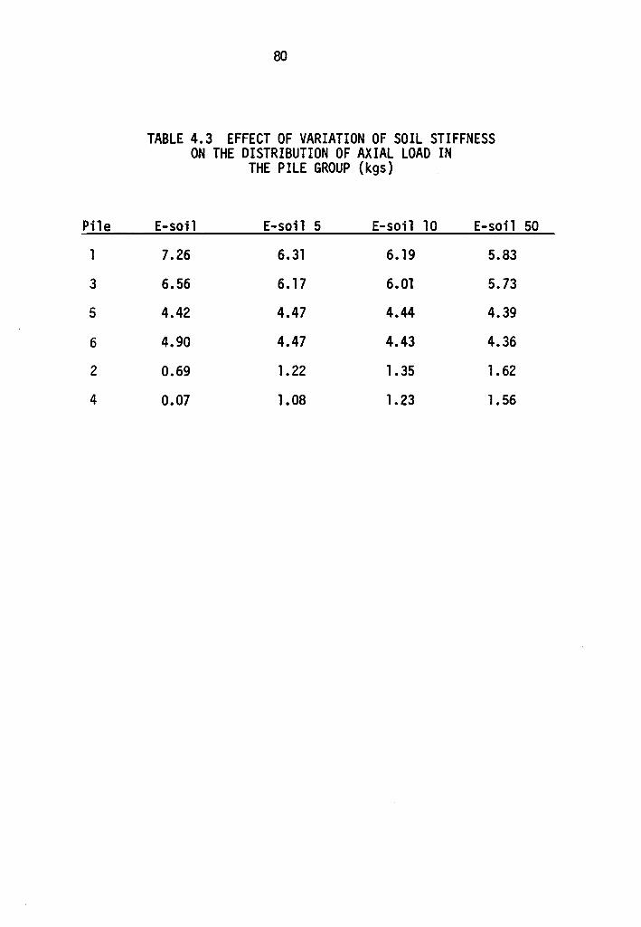
4.3 Effect of Variation of Soil Stiffness on the Distribution of Axial Load in the Pile Group 80
4.4 Effect of Variation of Pile Stiffness on the Distribution of Axial Load in the Pile Group 81
4.5 Effect of Variation of Plate Stiffness on the Distribution of Axial Load in the Pile Group 83
vii
a,. b
c
h
m
q
s, t
v
x, y, z
- - -x, y, z
E
Ek
Es
Et
Etf
Eti
Et.e. I
Mx' M_y
Mxx, Myy, Mxy
Pu
NOMENCLATURE
Dimensions of plate element.
Cohesion.
Thickness.
Length of beam-column element.
Ramberg-Os good Exponent.
Distributed load.
Local plate coordinates in x- and y- directions.
Local displacements in x-, y- and z-directions at node i.
Volume of an element.
Orthogonal, right handed, cartesian coordinates, in general.
Body Forces in x-, y- and z-directions.
Modulus of Elastici-e.y (F/L2).
Spring Stiffness (F/L).
Coefficient of Subgrade reaction (F/L3).
Soil modulus (F/L2}.
Final soil modulus (F/L2).
Initial soil modulus (F/L2).
Unloadind soil modulus (F/L2).
Moment of Inertia.
Beam bending moments in x- and y-directions.
Plate moment components in the xy system.
Ultimate soil resistance.
viii
Qx' QY S1
TX' Ty' T z
U, Ub' um
Vx' Vy w, wb' Wm
{ }, { }T
{q}' {qb}' {qm}
{r}, {r}
{ul
{Q}
{R} {R}
{T}
{X}
=t ] ' [ J T
[BJ , [Bbl, [Bm]
[CJ' [Cb]' [Cm]
[k)' [KJ_
[K]
[NJ' [Nal' [Nb]
ix
Shearing forces in plate. in x- and y-directions.
Surface on which tractions are specified.
Prescribed surface traction forces in x-, y-, and z-directions.
Strain energy, subscript b = bending case, subscript m = membrane case.
Shear in beam in x- and y-directions.
Potential energy of applied loads, b = bending case, m = ment>rane case.
A ·coluDll vector, the transpose of a column vector.
Local element displacenent vector, b = bending case, m = membrane case.
Global system displacenent vector,modified system displacement vector.
Local nodal displacement vector.
Local element force vector.
Global system force vector,modified global system force vector.
Vector of prescribed surface traction forces.
Vector of prescribed body forces.
A block matrix, the transpose of a matrix.
Strain-displacement matrix, subscript b = bending case, subscript m = membrane case.
Constitutive matrix, subscript b = bending case, subscript m = membrane case.
Local elenent stiffness matrix, global element stiffness matrix.
Modified element stiffness matrix.
Matrix of interpolation functions, subscript
y
&
'll'p' nb' '!I'm
anp' a'll'b' an m e . , Xl eyi' 9xyi
4>
{d, {~b}' h:m}
x
a = axial case, subscript m = meri>rane case.
Density.
Deflection.
Potential energy, subscript b = bending case, subscript m = meri>rane case.
Variation of potential energy.
Rotation about the x-axis, rotation about the y-axis, twist.
lnteTTtal angle of friction.
Strain vector, b = bending case, m = meri>rane case.
I. INTRODUCTION
Most Civil Engineering Structures are built on defonnable rock
and soil foundations. The defonnable characteristics of the soil
foundation and the rigidity (or flexibility) of the structure
mutually interact. That is, the deformation of the structure depends
upon not only its own rigidity {or flexibility) but also on the
characteristics of the interacting (soil) medium.
Closed form solution for some simple problems like a beam on
linear elastic foundation can be obtained. If the geometry of the
structure is nonuniform and the foundation medium is nonlinear, the
analysis becomes complex. Finite difference method can be employed to
analyze some situations. The finite element method is more versatile
and can include most of the factots easily. It can include irregular
geometry of the structure, nonlinearity of the foundation medium and
arbitrary loadind conditions.
In this study, a few selected soil-structure interaction
problems are analyzed by using finite element method. For this
purpose a computer code called FEM-STFN is used. The finite element
procedure idealizes the structure as an assemblage of two-dimensional plate elements and one-dimensional beam-column elements. The foundation
is replaced by spring elements. The spring stiffness is represented by
using Ramberg-Osgood model.
The problems solved involve beams and plates on elastic
foundations and pile group with cap. The problems solved include both
1
2
practical problems and nndel tests. Solutions of these problems by
different methods are available. These results are compared with
those obtained by the present analysis and discussed wherever
possible.
II. SOIL~STRUCTURE INTERACTION
2. l Introduction
Most Civil Engineering structures are built on defonnable soil and
rock foundations. Footings, rafts and pile foundations are some of the
structures whi~h interact with soil. The analysis of these structures
should be done by properly taking into account the 1111tual interaction
between the structure and the soil. The conventional method of founda-
tion design assumes arbitrary contact pressure distribution under the
structure. This assumption may not be valid because it does not take into
account the interaction effect. The interaction effect can be included
approximately by representing the soil by a set of discrete springs and
the resulting model is called Winkler's Model [23]. Winkler's Model is
a better model than the conventional method of analysis. However, in
Winkler's Model, the soil is represented by discrete independent springs
which can deform in the one (vertical) direction only. The effect in
the other (horizontal) direction due to the vertical load, that is,
Poisson's effect, is not included. The spring constant used in the
Winkler Model can be found from the coefficient of subgrade reaction of
the soil.
An improved model will be the elastic half space model [14]. If
actual stress-strain relationships of a foundation soil is incorporated
into the analysis of the half space model using non-linear theory, the
results can be closer to the actual situation. However, the approach
can be complex and as a result, the range of problems solved by this
manner is restricted. Still, the Winkler Model has some merits in
3
4
solving practical problems in a simple manner.
2.2 Coefficient of Subgrade Reaction [41,42]
The coefficient of subgrade reaction of soil, Es' is defined as the
ratio of soil resistance, q, to the deflection w required to develop the
resistance at a certain point. Thus
where
Es is in kN/m2/m
q is the pressure on the footing in kN/m2, and
w is the deflection at the point in meters.
2. 1
The coefficient of subgrade reaction can be evaluated from plate load
tests. Its value depends upon the soil properties, the size and the shape
of the plate used for the tests [41]. For preliminary designs, the range
of values of Es given by Terzaghi [41] as shown in Table 2.1 can be used.
When the Winkler Model is used to simulate non-linear soil behavior in
analyzing problems of laterally loaded piles and other structures, the
tangent spring modulus, Et' of the soil can be simulated from resistance-
deflection curves [14,35,36,37,38].
2.3 Resistance Deflection Curves The curves showing the soil resistance-deflection relationship (at
different depths} are called p-y curves. Different methods are available
to obtain these curves [14,32,35,36,37,38]. A general family of p-y
curves is shown in Figure 2.1. The curves imply that the soil re-
sistance depends upon the depth. Figure 2.2 shows the soil modulus at
5
TABLE 2.1
VALUES OF COEFFICIENT OF SUBGRADE REACTION Es' IN Kips/Cu. Ft., ON 1 Ft. x 1 Ft. SQUARE PLATE [41]
Sandy Soil
Dry or Moist Sand, Limiting Values
Proposed Values
Submerged Sand, Proposed
Clayey Soil
qu in Kips/Sq. ft.
Range of Values
Proposed Values
1 Kip/Cu. Ft. = 157.2 kN/m3
1 Ft. = 0.305 m
Relative Density of Sand
Loose Medium
40-120 120-600
80 260
50 160
Consistency of Clay
Stiff Very Stiff
2-4 4-8
100-200 200-400
150 300
•
Dense
600-2,000
1,000
600
Hard
8
400
600
FIG. 2.1
6
p
_]J --~·:_-Y
. I
~1 -1---Y -·
--;,- y
X : ·XI
GRAPHICAL REPRESENTATION OF p-y CURVES
(From Reference 36)
FIG. 2.2
7
I': \ \ ~ \
' l
\ \ ~ \ \ \ \· \
GRAPHICAL REPRESENTATION OF Et INCREASING WITH DEPTH (From Reference 35}
8
any point xi beneath the ground surface is a function of the load on the
pile and the deflection of the pile and increases linearlly with depth
[35]. The slope of a p-y curve at a point gives the tangent modulus Et.
Some empirical methods are available to construct p-y curves for
different soil types [14,37,38]. These methods depend on the pile
dimensions and the soil parameters c, + and y, where c is cohesion of
the soil in kN/m2, +is the angle of internal friction and y is the
density of the soil.
It should be noted that the p-y curves are not an inherent property
of the soil but a family of fitting functions to correlate the pile
deflection and soil properties at different depths. In this study, a
modified form [17] of the Ramberg-Osgood model [31] is used to represent
these p-y curves. A discussion of this model is given later in Chapter
III.
2.4 Beams on Elastic Foundations
is
where
The governing differential equation for a beam on elastic foundation
4 EI 3 + EtY = 0
dx
E = modulus of elasticity
I = moment of inertia
y = lateral movement
x = length of beam
Et = soil modulus
2.2
9
Closed-form solutions of various problems of beams on elastic founda-
tions were obtained by Hetenyi [23]. ·
Cheung and Nag [9] used the finite element method to study the
distribution of stresses in a beam on elastic foundation as well as the
vertical and horizontal contact pressure developed at the interface
between the beam and the foundation. In this method, the beam stiffness
matrix was obtained by the direct stiffness method and the foundation
stiffness matrix was obtained by inverting the flexibility matrix of the
foundation obtained from the equation of displacements of an isotropic
half-space [9,14]. The overall stiffness matrix of the foundation-structure
system is obtained by combining the two stiffness matrices. There are
three degrees of freedom at each node along the beam (u,w,ex) and only
two degrees of freedom at each node for the foundation (u,w) along the
line of interaction of the beam and the foundation. It is evident that
the force components, the displacement components and the stiffness
matrices for the beam and the foundation are not identical and a trans-
formation must be carried out before combining them. As it is sometimes
observed, an uplift may occur in flexible beams due" to the presence of
central loads which result in the presence of tensile contact pressure.
However, most foundation materials cannot carry tension and tend to
separate from the overlying structure. Cheung and Nag developed an iterative procedure to eliminate any tensile forces that may occur due
to loss of contact between the structure and the foundation. In this
method, whenever a tensile contact pressure is present at a certain
node, the rows and colunms in the foundation flexibility matrix cor-
10
responding to that node are made equal to zero and the new stiffness
matrix is obtained. : The procedure is repeated until no tensile contact
pressure occurs. However, this procedure may not be strictly correct.
It will be more correct to redistribute the negative pressure by an itera-
tive procedure without elimination.of soil stiffness. The procedure of
-,. redistributing negative pressures to compression zones is used in this
study and is explained later in Chapter III.
Haddadin [22] used the finite element procedure developed by Cheung
and Nag and solved a beam on elastic half space. He compared numerical
predictions with results obtained from a photoelastic study of a beam in
the laboratory.
2. 5 La tera 11 y Loaded Pjl es
The beam on elastic foundation theory can be used to analyze laterally
loaded piles. The lateral loads are applied at the top of the pile. The
spring constants representing the soil stiffness vary with depth depending
upon the nature of the soil.
A generalized closed-form solution of Eq. 2 .. 2 for laterally loaded
piles have been presented by Matlock and Reese [29]. In this method, the
solution is expressed as a combination of exponential and trigonometric
functions [14] and the final equation for displacement is
P T3 M T2 . t t 2 3 y = Er Ay + ~ By •
where y is the deflection, Pt and Mt are the applied lateral load and
moment respectively. T is the stiffness factor defined as
where
11
T = (EI/S0)l/S
E = modulus of elasticity of the pile
I = moment of inertia of the pile
s0 = Et/x, and
x = depth
2.4
AY and BY are dimensionless coefficients that are dependent on the pa-
rameters z = x/T and T. The slope, moment and soil reaction can then
be obtained by successive differentiation of Eq. 2.3. The results are
given in chart form in reference [29].
The analytical approach becomes highly complex when the pile
properties are irregular, that is E, I and diameter d, change, and the
soil properties are nonlinear. The finite difference method is often
used to solve laterally loaded pile problems including arbitrary variation
of pile geometry and nonlinear behavior of soil. Reese [34] presented a
procedure based on the finite difference method where p-y curves were
used to describe the nonlinear behavior of the soil. However, it is not
possible to include the effect of loading. and soil stiffness in all the
three·directions. The finite element method can easily take into account
most of these factors [14].
2.6 Plates on Elastic Foundations
The governing differential equation for plates on elastic founda-
tions is [44]
where
12
w = deflection
Es = coefficient of subgrade reaction Eh3
D = 2 12(1-v )
E = modulus of elasticity of plate
h = thickness
"' = Poisson's ratio of the material of the plate
q = load per unit area on the plate
2.5
A closed-form solution for an infinitely extended circular plate on
elastic foundation carrying a concentrated load at the center is available
[44]. However, the problem becomes highly complex for rectangular or
square plates on elastic foundation and the analytical procedure is very
cumbersome.
The finite difference method can be used for solving Eq. 2.5. How-
ever, this method can be quite cumbersome for plates with arbitrary change
in thickness and shape and nonlinear soil behavior.
The finite element method for the solution of plates on elastic
foundations have received.great attention because it is easy to account
for discontinuities and irregularities in the shape of the plate, dif-
ferent loading conditions and nonlinear behavior of soil. Severn [40]
attempted the solution of a plate on a Winkler foundation and added a
spring coupling action to s1111.1late shear resistance in the finite element
formulation.
13
Cheung and Nag (9] used a rectangular plate element to study the
contact pressure under a plate on elastic half-space. In this method,
the flexibility matrix of the soil was obtained from. the deflection
equations given by Boussinesq and Cerrutti [9,14]. The stiffness matrix
of the soil was obtained by inverting the flexibility matrix. Then the
stiffness matrix of the foundation was combined with that of the plate
to obtain the system stiffness matrix. They also investigated the effects
on the contact pressure due to loss of contact between plate and founda-
tion by eliminating all soil stiffness at nodes where uplift occurs.
Haddadin [21] developed a program to find the contact pressure for a
plate on a Winkler foundation by method of substructure. This method
takes into consideration the contribution of the superstructure to the
plate stiffness matrix. He used the same iterative method of Cheung and
Nag to eliminate ~he soil stiffness where tensile forces are developed.
However, this approach is not strictly correct because the stiffness
of the soil is arbitrarily eliminated where tensile pressures occur. A
more correct approach will be an iterative procedure by which the
negative pressures are redistributed into the system. This approach
is adopted in this study and explained later in Chapter III.
2.7 Pile Groups Hrennikoff [25] presented a method using matrix analysis to find the
load distribution in a pile group involving non-parallel piles where
both horizontal and vertical resistance of piles are considered. The
problem he presented is two dimensional. Aschenbrenner [2] extended the
method to a three-dimensional system with the piles assumed hinged to
14
the pile cap.
Reese, O'Neill and Smith [39] presented a method similar to that
of Aschenbrenner. In this method, it 1s assumed that the piles are
connected to a rigid pile cap. The connection is assumed to be rigid.
The internal nodal force vector and nodal displacement vector of each
pile are transfonned into an external nodal force vector and a nodal
displacement vector respectively by the following relations:
where
[Ai]{Fi} = {f(i)}
[Ai]T{X} = {6i}
[Ai] = transformation matrix for pile i
{Fi} = internal force vector at node i
{f(i)} =external force vector at node i
{X} =structure displacement.vector, and
{6i} = joint displacement vector at pile i
2.6
2.7
The pile-head stiffness matrix [Si] for each pile is defined as
Al 0 0 0 0 0
0 Bo 0 0 0 c 0 0 Bl 0 -c 0
[S.] = 2.8 l 0 0 0 G 0 0
0 0 -D 0 Fo 0
0 D 0 0 0 Fl
where
15
A1 = compression constant equal to AE/L or 2AE/L depending
on type of soil
B0 ,e1 = ~L; slope of the applied lateral-pile force vs.
deflection
G = torsion constant of the pile
C = Ph/e; the slope of pile-head force Ph necessary to restrain
translation when the correspdonding moments are applied.
D = ~h; slope of induced pile-end moment vs. deflection, and
F0 ,F1 = :; slope of pile-head rotation e in radians vs. moment.
The total structure stiffness matrix R is defined by
N [R] = t [Ai][Si][Ai]T
i=l
where N is the total number of piles in a group.
2.9
The footing displacement vector {X} is obtained from Eq. 2.10
below
{F} = [R]{X}
{X} = [R]-l{F} 2.lOa
2.lOb
where {F} is the external force vector that is applied on the footing.
Since {X} is known, substitution into Eq. 2.7 yields the displace-
ment vector for each joint. The pile-head reactions at each joint are
obtained from Eq. 2.6.
It should be noted that the stiffness matrix of the structure is a
6 x 6 matrix obtained by su11111ing up the contribution of the stiffnesses
of individual piles. The pile cap is assumed to be infinitely rigid and
the modulus of subgrade reaction of the soil is assumed to be constant.
16
A computer program using this method is given by Bowles [6] and used in
this study to compare the results of some.of the problems in Chapter IV.
The advantages of using the finite element analysis 1s that the
plates and beams with different properties. along their sections can be
modelled and the nonlinear soil behavior can be readily introduced in
the program. The presence of various boundary conditions as well as
notches and irregularities in plates can be easily accounted for without
much difficulty. Also, the elimination of tensile forces that develop
when an uplift occurs can be handled by redistributing these forces to
compressive areas via a simple stress transfer iteration scheme. It is
also quite easy to change the rigidity of the beams and plates as well
as the soil modulus to study the effect of these properties on the
general behavior of the soil-structure interaction problem.
III. THE FINITE ELEMENT MODEL
3.1 Introduction
The finite element method is a numerical technique to solve boundary
value problems by approximating a continuum as an assemblage of discrete
elements. Different types of elements are used to discretize a body such
as three-dimensional brick or tetrahedral elements, two-dimensional
quadrilateral or triangular. elements or one-dimensional beam-column
elements [11,13,14,26,47]. In this study, some problems on beams and
plates on elastic foundations, and pile groups are analyzed by using the
finite element method. One-dimensional beam-column elements and two-
dimensional rectangular plate elements are used to represent the struc-
ture. The supporting soil medium is represented by springs whose stiff-
ness depends upon the type of soil and depth of embedment. Details of
the finite element method are found in many books [11,13,14,26,47]; here,
only the salient features of the formulation of the beam-column element
and the rectangular plate element are given.
3.2 Beam-Column Element
A two node one-dimensional beam column element is shown in Figure
3. la. Each nodal point can have six degrees of freedom, three transla-
tional u, v and w; and three rotational ex, ey and ez. The element is subjected to transverse loads in the x- and y- directions, Figures
3.lc and 3.ld and axial load in the z-direction, Figure 3.lb.
For small strains and small axial loads compared to transverse
loads, one can consider the effects of the two to be uncoupled and the
17
8xl
vl ul
18
FIG. 3.la GENERAL ELEMENT
y
x z
FIG. 3.lc BENDING IN THE x- DIRECTION
x
FIG. 3.lb AXIAL LOAD
x FIG. 3.ld BENDING IN THE
y- DIRECTION
FIG. 3.1 GENERAL BEAM-COLUMN ELEMENT
(From Reference 11 )
19
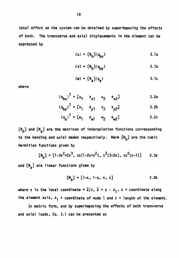
total effect on the system can be obtained by superimposing the effects
of both. The transverse and axial displacements in the element can be
expressed by
{u} = [Nb]{qbx} 3. la
{v} = [Nb]{qby} 3. lb
{w} = [Na]{qa} 3. le
where
{qbx}T = [u, 8xl u2 8x2] 3.2a
{qby}T = [vl eyl V2 ey2] 3.2b
{qa}T = [wl 8wl w2 8w2] 3.2c
[Nb] and [Na] are the matrices of interpolation functions corresponding
to the bending and axial modes respectively. Here [Nb] are the cubic
Hermitian functions given by
and [Na] are linear functions given by
[Na] = [1-s, 1-s, s, s] 3.3b
wheres is the local coordinate= z/1, z = z - z1, z =coordinate along
the element axis, z1 = coordinate of node l and 1 = length of the element.
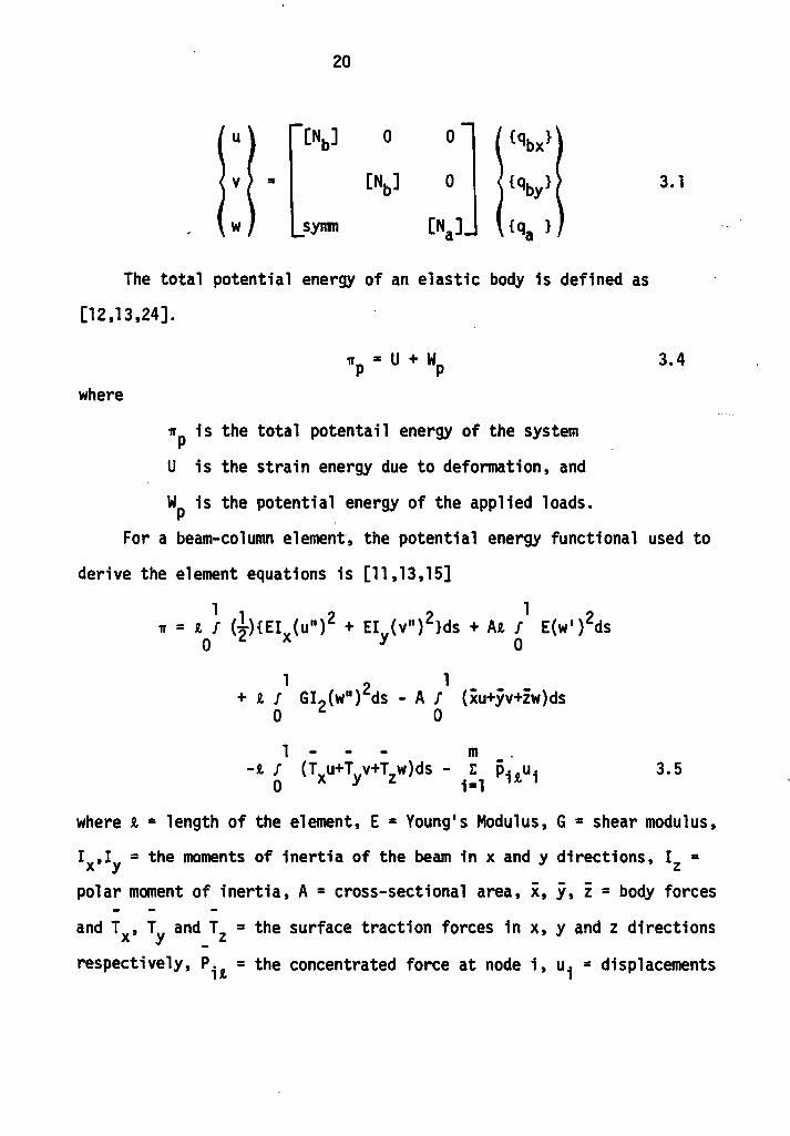
In matrix form, and by superimposing the effects of both transverse
and axial loads, Eq. 3.1 can be presented as
20
u [Nb] 0 0 {qbx}
v = [Nb] 0 {qby}
w synm [Na] {qa }
The total potential energy of an elastic body is defined as
[12,13,24].
where
'II' = u + w p p
np is the total potentail energy of the system
U is the strain energy due to deformation, and
WP is the potential energy of the applied loads.
3. l
3.4
For a beam-column element, the potential energy functional used to
derive the element equations is [11,13,15]
l 1 n = t I (1){EI (u")2 +EI (v")2lds +At I E(w 1
)2ds
0 2 x y 0
l l + t J GI2(w")2ds - A I (iu+yv+zw)ds
0 0
1 - m -t I (T u+T v+T w)ds - E p1.nu1• 0 x y z i=l h
3.5
where t = length of the element, E =Young's Modulus, G = shear modulus,
Ix,Iy = the moments of inertia of the beam in x and y directions, Iz = polar moment of inertia, A = cross-sectional area, i, y, z = body forces
and Tx, TY and_Tz =the surface traction forces in x, y and z directions
respectively, Pit= the concentrated force at node i, ui =displacements
21
at corresponding nodes (=u,v,w), and m =total number of degrees of
freedom where P; 1 is applied. The overbar denotes prescribed quantity.
The variational method used for the formulation of the element stiffness
matrix is based on the principle of minin11m potential energy [13].
Taking variation of the potential energy ~P with respect to the twelve
degrees of freedom {qi}' we obtain
a~P/a{q;l = o which leads to the equilibrium equation
[k]{q} = {Q}
where [k] = element stiffness matrix given by
ax[kx] [O] [O]
[k] = [O] ay[ky] [O]
[O] [O] [I),]
Elx -~ ax =3; a - 3 R, y 1
12 61 -12
4i -61 [k ] = [k ] = x y 12
S.Y11111
3.6
3.7
3.8a
61
2l
-61 3.Bb
412
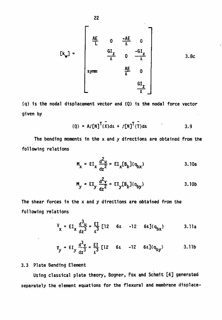
[k ] = w
22
AE L
synm
0 -AE R.
0
AE R.
3.8c
0
{q} is the nodal displacement vector and {Q} is the nodal force vector
given by
3.9
The bending moments in the x and y directions are obtained from the
following relations
The shear forces in the x and y directions are obtained from the
following relations
3 V = EI £!...H. = EI [12 6R. -12 x x dz3 ~
3 "I = El d v = EI [12 6R. -12 Y · Y dz3 ~
3.3 Plate Bending Element
3. lOa
3. lOb
3. lla
3.llb
Using classical plate theory, Bogner, Fox and Sc.hmit [4] generated
separately the element equations for the flexural and membrane displace-
23
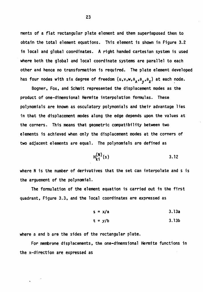
ments of a flat rectangular plate element and then superimposed them to
obtain the total element equations. This element is shown in Figure 3.2
in local and global coordinates. A right handed cartesian system is used
where both the global and local coordinate systems are parallel to each
other and hence no transfonnation is required. The plate element developed
has four nodes with six degree of freedom {u,v,w,ex,ey,ez) at each ~ode.
Bogner, Fox, and Schmit represented the displacement modes as the
product of one-dimensional Hermite interpolation formulas. These
polynomials are known as osculatory polynomials and their advantage lies
in that the displacement modes along the edge depends upon the values at
the corners. This means that geometric compatibility between two
elements is achieved when only the displacement modes at the corners of
two adjacent elements are equal. The polynomials are defined as
3.12
where N is the number of derivatives that the set can interpolate and s is
the arguement of the polynomial.
The formulation of the element equation is carried out in the first
quadrant, Figure 3.3, and the local coordinates are expressed as
s = x/a
t = y/b
where a and b are the sides of the rectangular plate.
3.13a
3.13b
For membrane displacements, the one-dimensional Hermite functions in
the x-direction are expressed as
24
z
(2,2)
FIG. 3 .2 PLATE ELEMENT IN LOCAL AND GLOBAL COORDINATES
25
y,t
(1,2) 1----------------, (2,2)
c b
a ~ x,s '-------------------------------~, (l, l) (2, l)
FIG. 3.3 FLAT RECTANGULAR PLATE ELEMENT *
* Arrow Indicates Sequence of Nodal Input
26
Ha~)(x) = l - s
Ha~) (x) = s
3. 14a
3. 14b
For bending displacements, the one-dimensional Hermite functions in
the x-direction are expressed as
Ha~)(x) = 2s3 - 3s2 + 1
Ha~)(x) = s2(3-2s)
H~~)(x) = as(s-1) 2
H~~)(x) = as2(s-l)
3. l Sa
3.lSb
3.lSc
3.lSd
By replacing x by y ands by tin Eqs. 3.14 and 3.15, expressions, for
Ha~)(y), Ha~)(y), Ha~)(y), Ha~)(y), Ht~)(y), and H~~)(y) are obtained.
The membrane displacements uij and vij as expressed in terms of
the Hermitian functions are
2 2 u(x,y) = r r Ha9)(x)Ha9)(y)u ..
i=l j=l 1 J lJ 3. l 6a
2 2 v(x,y) = r r Ha9)(x)Ha9)(y)v ..
i=l j=l 1 . J lJ 3.16b
where the subscripts 11, 12, 22 and 21 indicate nodes 1, 2, 3 and 4
respectively. Eq. 3.16 can be expressed as
3. 17
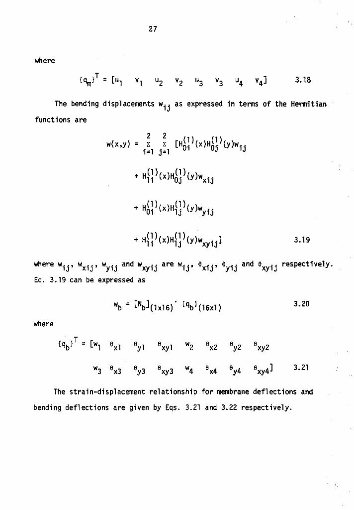
27
where
The bending displacements wij as expressed in tenns of the Hennitian
functions are
3.19
where wij' wxij' wyij and wxyij are wij' exij' eyij and exyij respectively. Eq. 3. 19 can be expressed as
wb = [Nb](lxl6) · {qb}(16xl) 3.20
where
{qb}T = [wl 6xl eyl 6xyl w2 6x2 ey2 6xy2
W3 6x3 ey3 6xy3 W4 6x4 ey4 6xy4] 3.21
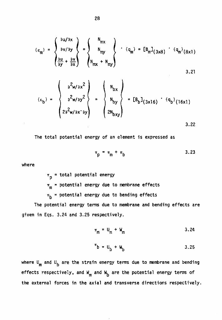
The strain-displacement relationship for membrane deflections and
bending deflections are given by Eqs. 3.21 and 3.22 respectively.
explained as follows. Because of the increased stiffness of the piles,
there will be less bending in the piles due to lateral movement. The
piles will tend to punch through the soil. Thus the structure can be
viewed as a stiff block rotating around the tip of the two piles battered
with the horizontal load causing most of the loads to be carried by these
piles.
Problem IV.7.lc - CASE III: Effect of variation of pile cap
modulus: Here initial soil modulus and modulus of elasticity of the
piles are kept constant. The modulus of elasticity of the pile cap is
increased by factors of 2, 3, 5 and 10 respectively. The results of
the study are given in Table 4.5. As shown, the solution is quite
sensitive to changes in the modulus of elasticity of the plate. As the
plate stiffness is increased the load is transferred to the piles that
are battered away from the horizontal load until the whole system be-
comes unstable and moves in a direction opposite to that of the applied
horizontal load. From the results given in Table 4.5, it is evident
that for this type of problem, the FEM-STFN code is very sensitive to
changes in the plate stiffness. The reason for this behavior may be
due to the dimensions of the pile cap. The plate element developed for
this study is considered to be a thin membrane element. However, the
ratio of length to height and width to height are 6:1 and 3.6:1,
respectively. Thus the basic assumption that the plate element is
thin does not hold. No final conclusion could be made with respect
to the effect of the variation of plate stiffness on the load distri-
bution in the pile group.
83
TABLE 4.5 EFFECT OF VARIATION OF PLATE STIFFNESS ON THE DISTRIBUTION OF AXIAL LOAD IN THE PILE GROUP (kgs}
Pile E-plate E-plate 2 E-plate 3 E-plate 5
1 7.26 6.64 5.35 3.88
3 6.56 6.21 5.30 3.81
5 4.42 4.52 4.41 4.33
6. 4.40 4.72 4.39 4.32
2 0.07 0.80 2.01 3.36
4 0.69 1.29 1.93 3.28
V. POSSIBLE EXTENSION
After studying the capabilities of the FEM-STFN code, the following
extensions are suggested.
1. Modification of the plate bending element to include
the effects of orthotropic material behavior.
2. Addition of the consistent mass matrix presented by
Bogner, Fox and Schmit [4]. Dynamic analysis can be
conducted.
3. Addition of a coordinate transfonnation matrix for
plate elements. This will eliminate the requirement
that the plate elements must be located in the x-y
plane. The analysis of shear wells subjected to
transverse loads can be conducted.
4. Provisions to include material nonlinearity.
5. Provisions to include different type of loading con-
ditions such as linearly varying transverse loads.
6. Addition of a subroutine for automatic mesh generation.
85
VI. CON:LUSIONS
In working with the FEM-STFN code and the literature studies,
the following conclusions are drawn:
1. The use of one-dimensional beam-column element and two-
dimensional Bogner, Fox and Schmit plate bending element
proved to be a very versatile tool in handling problems
of beams and plates on elastic foundations as well as
pile groups.
2. The idealization of the soil medium as a set of springs
is easy to program and the results are accurate enough
for the present type of analysis.
3. The stress transfer scheme developed herein takes into
account the overall stiffness of the foundation. It is
felt that this scheme i.s better than the one developed
by Cheung and Nag (9) where the soil medium is completely
neglected when an uplift occurs.
4. With the modifications proposed earlier, the program is
able to handle a wide variety of soil-structure inter-action problems faced by the engineer.
86
REFERENCES
l. Anandakrishnan, U.,' Kuppusall\Y, T., and Krishnaswall\Y, N. R., Design Manual for Raft Foundations, Department of Civil Engineering, Indian Institute of Technology, Kanpur, India, 1971.
2. Aschenbrenner, R., "Three Dimensional Analysis of Pile Foundations," Journal of Structural Division, ASCE, Vol. 93, STl, Feb., 1967.
3. Bandyopadhyay, M., "A Finite Element Analysis of Plate and Shell Structures," thesis presented to the Virginia Polytechnic Institute and State University, at Blacksburg, Virginia, in 1976, in partial fulfillment of the requirements for the degree of Master of Science.
4. Bogner, F. K., Fox, R. L. and Schmit, L. A., Jr., "The Generation of Interelement Compatible Stiffness and Mass Matrices by the Use of Interpolation Formulas," Proceedings of the First Conference on Matrix Methods in Structural Mechanics (26-28 October 1965}, A.F.I.T., Wright-Patterson Air Force Base, Ohio, 1966.
5. Bowles, J. E., Foundation Analysis and Design, McGraw-Hill Book Company, New York 1968.
6. Bowles, J. E., Analytical and Computer Methods in Foundation Engineering, McGr~w-Hill Book Company, New York, 1974.
7. Butterfield, R. and Bannerjee, P. K., "The Problem of Pile-Groups Pile Cap Interaction," Geotechnique, Vol. 21, No. 2, 1971.
8. Cheng, A. P. and Fun, H. L., "Beams on Discrete, Nonlinear Elastic Supports, 11 J. of Struct. Div., Proceedings of the ASCE, Sept., 1969.
9. Cheung, Y. K. and Nag, D. K., "Plates and Beams on Elastic Foundations: Linear and Nonlinear Behavior, 11 Geotechnique, June, 1968.
10. Cheung, Y. K. and Zienkiewicz, O. C., "Plates and Tanks on Elastic Foundation: An Application of Finite Element Method, 11 Int. J. Solids Struct., Vol. 1, 1965.
11. Desai, C. S., Elementary Finite Element Method, Prentice-Hall, Inc., Englewood Cliffs, New Jersey, 1978-79.
12. Desai, C. S., "A Three-dimensional Finite Element Procedure and Computer Program for Nonlinear Soil-Structure Interaction," VPl&SU Dept. Civ. Eng., Rep. VPI-E-75-27, Blacksburg, Va., June, 1975.
13. Desai, C. S. and Abel, J. F., Introduction to the Finite Element Method, Van Nostrand Reinhold Company, 1972.
87
14. Desai, C. S. and Christian, J. T., Numerical Methods in Geotechnical Engineering, McGraw-Hill Book Company, New York, 1977.
15. Desai, C. S. and Kuppusamy, T., "A Computer Code for Axially and Laterally Loaded Piles and Retaining Walls," Report, Department of Civil Engineering, Virginia Polytechnic Institute and State University, Blacksburg, Virginia, 1978.
16. Desai, C. S. and Patil, U. K., "Finite Element Analysis of Building Frames and Foundations," Report, Department of Civil Engineering, Virginia Polytechnic Institute and State University, Blacksburg, Virginia, 1976-1977.
17. Desai, C. S., and Wu, T. H., "A General Function for Stress-Strain Curves," Proc. 2d Int. Conf. Numer. Methods Geomech., Blacksburg, Va., June 1976.
18. Durelli, A. J., Parks, V. J., Mok, C. C. and Lee, H. C., "Photoelastic Study of Beams on Elastic Foundations," Proc. ASCE, J. St. Div., Vol. 95, ST8, Aug., 1969.
I
19. Felippa, C. A. and Tocher, J. L., "Discussion: Efficient Solutfon of Load-Deflection Equations," Journal of Structural Division, ASCE, Feb., 1970. .
20. Fruco and Associates, "Pile Driving and Loading Tests: Lock and Dam No. 4, Arkansas River and Tributaries, Arkansas and Oklahoma," U. S. Army Corps of Engineers District, Little Rock, Sept., 1964.
21. Haddadin, M. J., "Mats and Combined Footings: Analysis by the Finite Element Method," ACIJ, pp. 954-969, 1971.
22. Haddadin, M. J., "Discussion: Photoelastic Study of Beams on Elastic Foundations," Proc. ASCE, J. Struct. Div., Vol. 96, ST4, April 1970.
23. Hetenyi, M., Beams on Elastic Foundations, University of Michigan Press, Ann Arbor, 1946.
24. Holzer, S. M., "Lecture Notes on CE 4001-2, Matrix Structural Analysis," Department of Civil Engineering, Virginia Polytechnic Institute and State University, Blacksburg, Virginia, 1978.
25. Hrennikoff, A., "Analysis of Pile Foundations with Batter Piles, 11
Proceedings, ASCE, Vol. 75, 1949.
26. Huebner, K. H., The Finite Element Method for Engineers, John Wiley and Sons, New York, 1975.
88
27. Mastrogeorgopoulos, S. C., "Finite Element Analysis of Orthotropic Plates with Eccentric Stiffeners," dissertation presented to the Virginia Polytechnic Institute and State University, at Blacksburg, Virginia in 1972, in partial fulfillment of the requirements for the degree of Doctor of Philosophy.
28. Malek, K. A., "Design and Analysis of Two-story Buildings, 11 Project submitted to the Virginia Polytechnic Institute and State Univer-sity, at Blacksburg, Virginia, in 1976, in partial fulfillment of the requirements for the degree of Master of Engineering in Civil Engineering.
29. Matlock, H., and Reese, L. C., 11 General ized Solutions for Laterally Loaded Piles,"Trans. ASCE, Vol. 127, pt. 1, 1962.
30. McGonaghy, J.M., "Finite Element Analysis of Rectangular Orthotropic Plates, 11 project report presented to the Virginia Polytechnic Institute and State University, at Blacksburg, Virginia, in 1978, in partiall fulfillment of the requirements for the degree of Master of Engineering.
31. Ramberg, W. and Osgood, W. R., "Description of Stress Strain Curves by Three Parameters," National Advisory Co11111ittee for Aeronautics, Technical Note 902, Washington, D. C., 1943.
32. Reese, L. C., "Discussion of 'Soil Nodulus for Laterally Loaded Piles' by Mccelland and Foct, 11 Transactions, ASCE, Vol. 123, 1958.
33. Reese, L. C., "Ultimate Resistance against a Rigid Cylinder Moving Laterally in a Cohesionless Soil, 11 Society of Petroleum Engineers Journal, Dec., 1962.
34. Reese, L. C., "Laterally Loaded Piles: Program Documentation," Jl. Geot. Eng. Div., ASCE, Vol. 103.
35. Reese, L. C. and Cox, W. R., "Soil Behavior from Analysis of Tests of Uninstrumented Piles under Lateral Loading, 11 ASTM Spec. Tech. Pub. 444, 1969.
36. Reese, L. C., Cox, W. R., and Koop, F. D., "Analysis of Laterally Loaded Piles in Sand, 11 Sixth Offshore Technology Conference, Houston, Texas, 1974 .•
37. Reese, L. C., Cox, W.R., and Koop, F. D., "Analysis of Laterally Loaded Piles in Stiff Clay, 11 Seventh Offshore Technology Conference, Houston, Texas, 1975.
38. Reese, L. C. and Matlock, H., "Non-dimensional Solutions for Laterally Loaded Piles with Soil Modulus Assumed Proportional to Depth, 11
Proceedings of the Eighth Texas Conference, Society of Mechanical Foundation Engineering, University of Texas, 1956.
89
39. Reese, L. C., O'Neill, M. w., and Smith, R. E., "Generalized Analysis of Pile Foundations," Journal of the Soil Mechanics and Foundation Division, ASCE, Jan. 1970.
40. Severn, R. T., "The Solution of Foundation Mat Problems by Finite Element Method," Struct. Eng., Vol. 44, No. 6, 1966.
41. Terzaghi, K., Theoretical Soil Mechanics, John Wiley and Sons, Inc., New York, 1943.
42. Terzaghi, K., "Evaluation of Coefficients of Subgrade Reaction," Geotechnique, Vol. 5, Dec., 1955.
43. Timoshenko, S., Strength of Materials, Van Nostrand Reinhold Company, Princeton, l956.
44. Timoshenko, S. and Woinowsky-Krieger, S., Theory of Plates and Shells, McGraw-Hill Book Company, Second Edition, New York, 1959.
45. Winterkorn, H. F. and Fang, H. Y., Foundation Engineering Handbook, Van Nostrand Reinhold Company, New York, 1975.
46. Yang, T. Y., "Flexible Plate Finite Element on Elastic Foundation," J. Struct. Div. Proc. ASCE, Vol. 96, No. STlO, Oct. 1970.
47. Zienkiewicz, O. C., The Finite Element Method in Engineering Science, McGraw-Hill Book Company, Second Edition, London, 1971.
48. Zienkiewicz, O. C. and Cheung, Y. K., "The Finite Element Method for the Analysis of Elastic Isotropic and Orthotropic Slabs, 11 Proc. Inst. Civ. Eng., Aug. 28, 1964.
The vita has been removed from the scanned document
FINITE ELEMENT ANALYSIS OF SOME SOIL~STRUCTURE INTERACTION PROBLEMS
by
Ahmad Raif Alameddine
(ABSTRACT}
A finite element procedure is used for analysis of a number of
soil-structure interaction problems. This procedure involves one-