Finite Element Design and Manufacturing of a Nylon-String Guitar Soundboard from Sandwich-Structured Composites Negin Abaeian Music Technology Area, Department of Music Research Schulich School of Music McGill University Montreal, Canada December 2017 A thesis submitted to McGill University in partial fulfillment of the requirements for the degree of Master of Arts c 2017 Negin Abaeian
Transcript
Finite Element Design and Manufacturing of aNylon-String Guitar Soundboard from
Sandwich-Structured Composites
Negin Abaeian
Music Technology Area, Department of Music Research
Schulich School of Music
McGill University
Montreal, Canada
December 2017
A thesis submitted to McGill University in partial fulfillment of the requirements for the degree ofMaster of Arts
c� 2017 Negin Abaeian
i
Abstract
The aim of this project was to use the Finite Element Method (FEM) to design and manu-
facture the soundboard of a nylon-string guitar from sandwich-structured composites, with
reference to an existing wooden soundboard, and to evaluate the accuracy of the numeri-
cal models of the wooden soundboard, the brace-less composite top plate and the braced
composite soundboard by means of experimental modal analysis.
The modal behaviour of the existing wooden soundboard was studied through experi-
mental modal analysis and numerical simulation. Using FEM, the e↵ects of varying certain
physical, geometric and elastic properties of the materials used in the soundboard were de-
termined on its natural frequencies under free and hinged Boundary Conditions (BCs). The
composite soundboard that was determined to have natural frequencies relatively similar to
those of the wooden soundboard under hinged BCs, and could be built from commercially
available materials was constructed. To verify the results predicted numerically, experimen-
tal modal analyses were performed on the brace-less composite top plate and the braced
composite soundboard under free BCs.
The experimental natural frequencies and mode-shapes of the constructed brace-less top
plate were found to match those predicted by the simulation in the frequency range below
200 [Hz], while slightly diverging in the higher frequency range. The experimental results
for the braced composite soundboard were also found to be relatively similar to the nu-
merically predicted values, with most mode-shapes matching, and some di↵erences in the
mode-frequencies, mostly in the low and mid-frequency ranges. Overall, a reasonable agree-
ment was achieved between the numerical and the experimental results.
ii
Sommaire
L’objectif de ce projet etait d’utiliser la Methode des Elements Finis (MEF) pour concevoir et
fabriquer une table d’harmonie de guitare a cordes en nylon a partir de composites sandwiches
en se referant a une table en bois existante; et d’evaluer la precision des modeles numeriques
de la table d’harmonie en bois, de la plaque superieure en composite sans renforts et de la
table d’harmonie composite renforcee au moyen d’une analyse modale experimentale.
Le comportement modal de la table d’harmonie existante en bois a ete etudie au moyen de
l’analyse modale experimentale et de la simulation numerique. En utilisant la MEF, les e↵ets
de la variation de certaines proprietes physiques, geometriques et elastiques des materiaux
utilises dans la table d’harmonie ont ete determines sur ses frequences propres en utilisant
des Conditions aux Limites (CL) soit libres soit immobiles (c.a-d., sans translations). La
table d’harmonie en composite, dont on a determine qu’elle avait des frequences propres
relativement similaires a celles de la table d’harmonie en bois sous CL immobiles, et qui
peut etre construite a partir de materiaux disponibles dans le commerce, a ete produite.
Pour verifier les resultats predits numeriquement, des analyses modales experimentales ont
ete e↵ectuees sur la plaque superieure composite et la table d’harmonie en composites sous
CL non contraintes.
Les frequences propres experimentales et les di↵erents modes propres de la plaque superieure
construite sans renforts correspondent a celles predites par la simulation dans la gamme
de frequences inferieures a 200 [Hz], tout en divergeant dans la plage de frequences plus
elevees. Les resultats experimentaux pour la table d’harmonie composite avec renforts se
sont egalement reveles relativement similaires aux valeurs predites numeriquement, la plupart
des formes de modes propres correspondantes, et certaines di↵erences dans les frequences pro-
pres, principalement dans les plages de basses et moyennes frequences. Dans l’ensemble, un
accord raissonable a ete obtenu entre les resultats numeriques et les resultats experimentaux.
iii
Acknowledgements
First and foremost, I would like to thank Dr. Gary Scavone for his support, counsel and
believing in me all along, and for providing the space and the equipment required for my
research. I would also like to thank Dr. Larry Lessard for his guidance and for allowing
me access to the Structures and Composite Materials Laboratory facilities and the materials
needed for this project.
I want to thank Joel Barbeau for making two wooden soundboards and allowing me
to perform experiments on them. This project would not have been possible without his
help. I would also like to thank Ulrich Blass, my companion in the first half of this project.
It was also with his help that a portion of the experimentation and construction stages
were carried out. Next, I would like to thank Evonik Industries for providing me with the
foams needed for the construction of the guitar soundboard. I then want to extend my
appreciation to Marion Paris and Vincent Cadran for translating the abstract of this thesis,
Matteo Putt for sharing his technical knowledge on composites, and all of them for helping
me in the construction and experimentation stages. Many thanks to Esteban Maestre and
the members of the Computational Acoustic Modelling Laboratory (CAML) for sharing their
knowledge and insight, as well as the members of the Structures and Composite Materials
Laboratory for accepting me as a member of the lab. Last but not least, I want to thank
my family for their endless support through hard times during the course of this project.
4.3 Mass of the Top Plates: Simulation vs. Experimental . . . . . . . . . . . . . 91
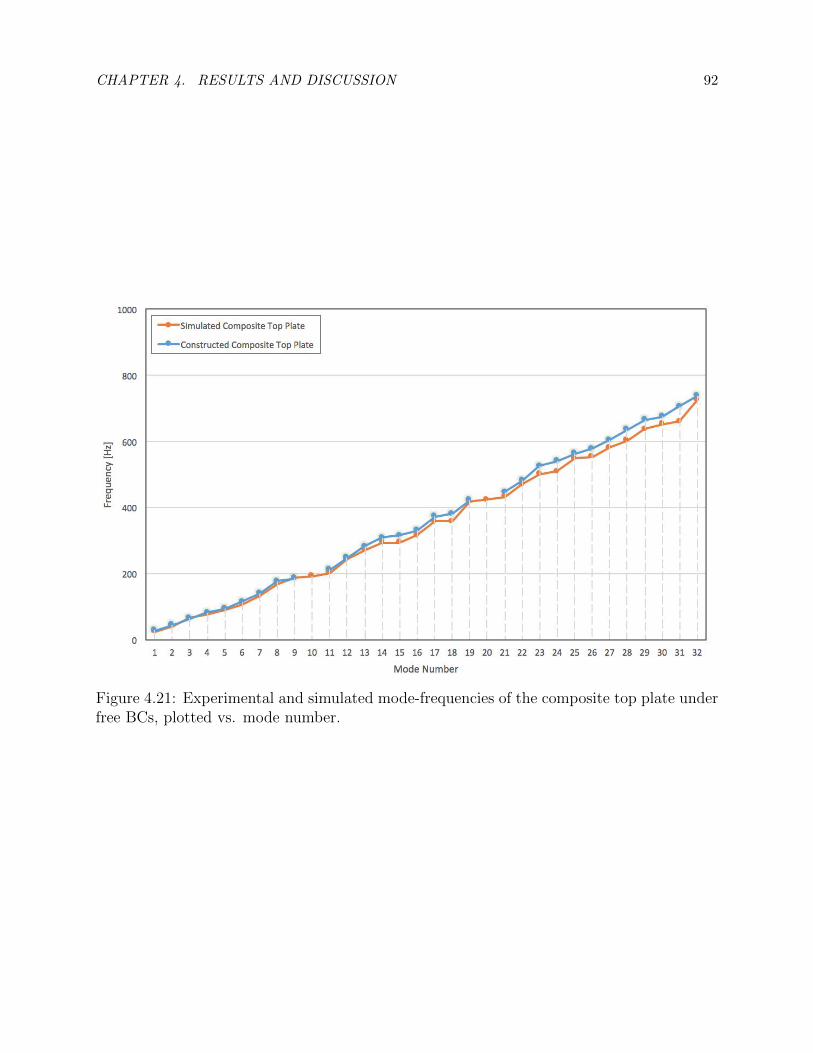
4.4 Simulation and Experimental Mode-Frequencies of the Composite Top Plate 93
4.5 Mass of the Soundboards and the Braces . . . . . . . . . . . . . . . . . . . . 96
4.6 Simulation and Experimental Mode-Frequencies of the Composite Top Plate 99
x
List of Abbreviations
CAD: Computer Aided Design
DOF: Degrees of Freedom
EOM: Equation of Motion
FEM: The Finite Element Method
FRP: Fiber Reinforced Plastics
CFRP: Carbon Fibre Reinforced Plastics
GFRP: Glass Fibre Reinforced Plastics
ODS: Operational Deflection Shape
MSDS: Material Safety Data Sheet
xi
Chapter 1
Introduction
1.1 Motivation
The vibrational behaviour of the nylon-string guitar is a function of di↵erent factors that
intrinsically a↵ect the sound quality or the musical timbre of the instrument. One of the
most important factors is the top plate of the instrument (i.e., the soundboard), since the
sound produced by an acoustic plucked-string instrument, such as the guitar, highly depends
on the ability of the soundboard to vibrate in response to the strings’ excitation [1, p.11].
For hundreds of years, the body of the nylon-string guitar and the braces inside the
body have been made mainly from wood. Many tonewoods, however, are now on the verge
of extinction [2]. In addition to that, since wood is a natural material, it is not possible
to re-produce a wooden guitar with identical elastic properties, vibrational behaviour and
consequently the same timbre as another. Di↵erent wooden species or parts belonging to the
same trunk may not exhibit identical extents of variations, nor do they behave in the same
manner under identical excitations. Furthermore, the response of wooden instruments can
vary with humidity and temperature [1, p.235].
It is due to this sensitivity to environmental changes, lack of predictability in the in-
strument sound, and sustainability factors that many acoustic guitar makers have started
exploring the possibility of producing instruments from more stable and predictable synthetic
materials such as composites. Examples of composite guitars commercially available in the
market would include Ovation Guitars, which have been in the market since the 1960’s [3],
as well as RainSong [4, p.37] and Emerald guitars [5]. Aside from the commercial gui-
tars available in the market, a number of custom-made composite guitars and their acoustic
properties have been studied by other researchers as well, e.g. [6] [7] [8].
1
CHAPTER 1. INTRODUCTION 2
Despite the research done on composite guitars, the musical benefits and acoustic prop-
erties of composites as substitute materials for wood are still rather unknown to many
musicians. Therefore, the ultimate goal of this project was to expand the research and lit-
erature available on the vibrational properties of composite instruments, and to explore the
possibility of making composite guitars that sound similar to conventional wooden guitars.
1.2 Project Overview
The aim of this project was to use the Finite Element Method (FEM) to design and manu-
facture the soundboard of a nylon-string guitar from sandwich-structured composites, with
reference to an existing wooden soundboard, and to evaluate the accuracy of the numeri-
cal models of the reference and the designed soundboards by means of experimental modal
analysis.
The composite soundboard was designed such that it is strong enough to withstand the
tension of the strings, light enough to vibrate in response to conventional strings, and under
hinged Boundary Conditions (BCs), has natural frequencies similar to those of the wooden
soundboard. It was therefor required that the design takes both static and vibrational
properties of the soundboard into account. In order to minimize the e↵ect of other factors
in this material substitution, the soundboard was treated independently, and the pattern of
the braces behind the soundboard was left unchanged.
A wooden soundboard intended for a flamenco guitar was borrowed from Joel Barbeau, a
Montreal-based guitar luthier, and was treated as the reference for the design. A numerical
model of the soundboard was made and the results of the finite element simulations were
regarded as theoretical results. For verification purposes, a series of experimental modal
analyses were performed on the wooden soundboard, as well as on the manufactured brace-
less composite top plate and the braced composite soundboard.
1.3 Thesis Overview
Chapter 2 of this thesis will provide the background information required for understand-
ing the terminology and the theories used throughout the project, from material science
to theoretical and experimental modal analyses, followed by a literature review on guitar
soundboard acoustics, composite materials and composite instruments.
CHAPTER 1. INTRODUCTION 3
Chapter 3 will explain the thought process and the steps taken throughout the design,
construction and experimentation stages.
Chapter 4 presents and analyzes the theoretical and experimental results obtained at
di↵erent stages. The analyses will elaborate why certain decisions were made in the design
process, and whether the experimental results match those predicted by the simulations.
Furthermore, the limitations in the proposed methodology and the design will be discussed,
as well as the sources of error.
Chapter 5 will close the report by summarizing the results and the conclusions of the
project, followed by the further potential work suggested.
It must be noted that during the first 6 months of this project, I was involved in the design
and construction of a composite steel-string guitar soundboard as well, in collaboration with
Ulrich Blass, a visiting researcher from the Technical University of Kaiserslautern. He was
a part of the Structures and Composites Laboratory of McGill at the time. A portion of the
experiments and designs were therefore performed collaboratively, which is why this report
is written in a first person plural voice.
1.4 Contributions
The thesis in hand sheds light on the e↵ects of varying certain physical, geometric and
elastic properties of the materials used in sandwich-structured composite soundboards on
their natural frequencies and mode-shapes. It also discusses the di↵erences observed between
the experimental and the numerical results and the possible sources of error.
Another observation that is briefly documented in this thesis is the variations of the
modal parameters of the wooden soundboard over time. This phenomena is thought to be
caused by environmental factors like temperature and humidity, and it further motivates us
to consider producing instruments from synthetic materials that are less sensitive to humidity
and temperature.
The outputs of this project broaden our understanding of the factors that a↵ect the modal
parameters of a guitar soundboard, providing a more solid ground for further research on
numerical modelling of sandwich-structured composites and composite soundboard designs.
Chapter 2
Background
The instruments belonging to the current family of guitars vary in a number of structural
aspects that result in variations in the timbre, vibrational and acoustical properties of the
instrument. In order to narrow down the scope of this project, the following history and the
principles provided will focus on the conventional nylon-string guitar, and more specifically,
on their soundboards.
2.1 Relevant History
2.1.1 Nylon-String Guitars
The modern nylon-string guitar as we know it was predominantly the invention of Antonio
de Torres in the 19th century [9]. Although the family of lutes, necked string instruments [4,
p. 2] and guitar-like instruments date back to centuries prior to that, it was since Torres’s
designs that a number of features remained standardized in the modern guitar. Despite
their variations, the consistent features in his guitars were the presence of 6 strings, the
body silhouette, the fretboard being raised above the soundboard [4, p. 14] and joined to
the body at the 12th fret, geared tuners and most importantly, the fan bracing behind the
soundboard [9].
Aside from Torres’ design, many other guitar designs have been explored since the 19th
century. Fig. 2.2 shows examples of some bracing pattern variations for the nylon-string
guitar that have been developed over the years. Notice that not all bracing patterns used
for acoustic guitars have a symmetric layout.
4
CHAPTER 2. BACKGROUND 5
Figure 2.1: Examples of Torres patterns. From left to right: models FE 19, SE 70, SE147 [10, p. 116].
Figure 2.2: Alternate bracing pattern examples. From let to right: Radial bracing by RandyReynolds [11], Kasha design [4, p. 19], and lattice design by Chris Pantazelos for a 7 stringguitar [4, pp. 20].
The ultimate aim of every guitar soundboard is to be light enough to vibrate in response
to the excitation of the strings, yet maintain adequate strength and sti↵ness to not fail under
the tension of the strings [4]. Achieving this goal is the art of the luthier and can be achieved
in more than one way. Kasha’s design in Fig. 2.2, for instance, is intended to distribute the
torque caused by the strings across the rest of the body, also causing the di↵erent regions of
the soundboard to have di↵erent resonances. A more recent example is the lattice bracing
pattern, that gives a distributed sti↵ness to the soundboard.
CHAPTER 2. BACKGROUND 6
The variations in guitar designs are not limited to the bracing patterns. Instruments
belonging to the guitar family can vary in the number of strings, body silhouette and size,
the materials used in the di↵erent parts, location and size of the sound hole, number of
sound holes, scale length, bridge design, etc. Below are a few alternate guitar designs. In
Fig. 2.3, the lattice bracing is made of a CFRP/balsa sandwich, providing high sti↵ness to
the soundboard. The second guitar in this figure is an example of a concert guitar with a
non-conventional sound-hole location [12], and the soundboard on the right is a double-top
soundboard. Double-top soundboards are made from a sandwich configuration consisting of
two usually dissimilar layers of wood and a thin and light honey-comb layer as the core.
Figure 2.3: Lattice CFRP/balsa bracing [4, p. 114], nylon-string guitar with an unconven-tional sound hole location [12], Double top guitar [13].
The acoustic results of new designs and variations are rarely predicted prior to con-
struction, and in most cases, they are not analyzed following production either. Although
researchers have attempted to come up with more standardized ways of categorizing gui-
tars [14] [15] or assessing their components based on their structural characteristics and
vibrational behaviour, luthiers still mainly rely on their experience and qualitative observa-
tions in evaluating the make of a guitar and its components.
2.1.2 Composite Instruments
Composites o↵er a number of desirable material properties, namely, high sti↵ness, durability,
and less sensitivity to humidity and temperature changes, as well as being able to mould
to complex shapes. These features make them suitable candidates for applications in many
CHAPTER 2. BACKGROUND 7
industries, such as aviation and automobiles. In the realm of musical instruments, although
composite materials are not widely used yet, their use in the di↵erent parts of string and
non-string instruments has been explored by researchers and luthiers in the past several
decades. Many of these composite instruments are now available in the market.
The first commercial appearance of composites in musical instruments dates back to the
1960’s, when Ovation Guitars started using Glass Fibre Reinforced Plastics (GFRPs) in the
body of acoustic guitars. [4, p. 24]. Other composite guitars that have been commercially
available since then are produced by Rainsong, since the 1990’s, Emerald Guitars, since the
2000’s [5], and more recently by Blackbird, Journey Instruments, Mcpherson, The Cargo and
KLOS. [16]. The bodies of these acoustic guitars are made from Carbon Fibre Reinforced
Plastics (CFRPs), but they vary in size, shape, composite thickness, location and number of
sound holes, etc. There are also other acoustic guitars commercially available that are not
entirely made from composites, but contain composite components. An example would be
the fingerboard of some Gibson Guitars that are made from CFRPs [17].
Figure 2.4: Left: an Ovation guitar with uni-directional GFRP soundboard and the backmade of Lyracord [3]. Centre: a brace-less Rainsong guitar with an all-body graphite body[18]. Right: Emerald X20 nylon-string made from a sandwich-structured woven CFRP [19].
CHAPTER 2. BACKGROUND 8
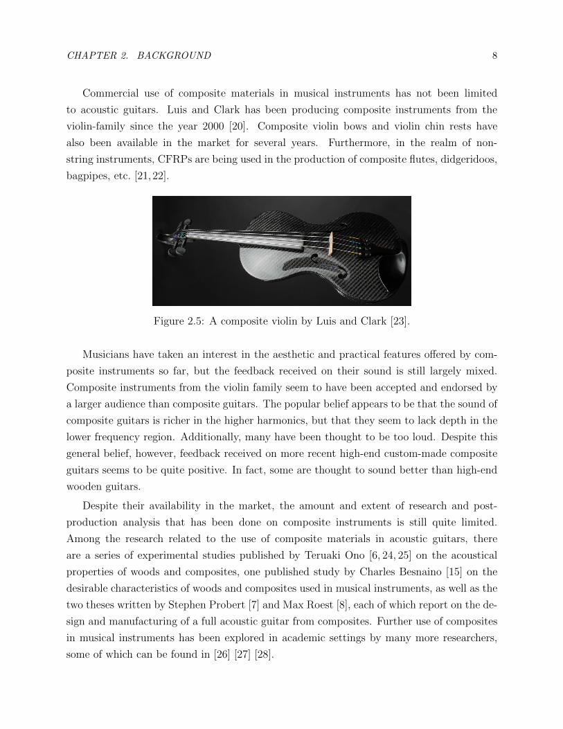
Commercial use of composite materials in musical instruments has not been limited
to acoustic guitars. Luis and Clark has been producing composite instruments from the
violin-family since the year 2000 [20]. Composite violin bows and violin chin rests have
also been available in the market for several years. Furthermore, in the realm of non-
string instruments, CFRPs are being used in the production of composite flutes, didgeridoos,
bagpipes, etc. [21, 22].
Figure 2.5: A composite violin by Luis and Clark [23].
Musicians have taken an interest in the aesthetic and practical features o↵ered by com-
posite instruments so far, but the feedback received on their sound is still largely mixed.
Composite instruments from the violin family seem to have been accepted and endorsed by
a larger audience than composite guitars. The popular belief appears to be that the sound of
composite guitars is richer in the higher harmonics, but that they seem to lack depth in the
lower frequency region. Additionally, many have been thought to be too loud. Despite this
general belief, however, feedback received on more recent high-end custom-made composite
guitars seems to be quite positive. In fact, some are thought to sound better than high-end
wooden guitars.
Despite their availability in the market, the amount and extent of research and post-
production analysis that has been done on composite instruments is still quite limited.
Among the research related to the use of composite materials in acoustic guitars, there
are a series of experimental studies published by Teruaki Ono [6, 24, 25] on the acoustical
properties of woods and composites, one published study by Charles Besnaino [15] on the
desirable characteristics of woods and composites used in musical instruments, as well as the
two theses written by Stephen Probert [7] and Max Roest [8], each of which report on the de-
sign and manufacturing of a full acoustic guitar from composites. Further use of composites
in musical instruments has been explored in academic settings by many more researchers,
some of which can be found in [26] [27] [28].
CHAPTER 2. BACKGROUND 9
The study published by Charles Besnainou attempts to categorize wooden guitars and
violins based on their acoustical properties and introduces principles that must be taken
into account when designing acoustic instruments from composites. His statements are later
used, verified and extended in the literature of composite instruments that will be presented
in Sec. 2.5.
Teruaki Ono’s design was the final stage of a series of experimental studies by him and
his team that revealed the acoustical properties of di↵erent woods and sandwich-structured
FRP configurations. His final design is the layup shown below, where CF(L)/UF refers to
carbon fiber filaments laid longitudinally in a polyurethane foam matrix, CF(R)/UF refers
to carbon fiber filaments laid in the perpendicular direction in a polyurethane foam matrix,
and UF is a layer of polyurethane foam alone. The Frequency Response Functions (FRFs)
obtained from the produced guitar were found to be very close to those of the reference
wooden guitar.
Figure 2.6: Layup of the composite guitar made by Ono [6].
Stephen Probert used numerical simulation to design and manufacture a full steel string
guitar in his Master’s thesis. His design makes use of a sandwich-structured CFRP with a
foam core. On each side of the core, two layers of standard woven CFRPs are used: one at
a 0/90� angle, and the other at a 45� angle. It is stated that the guitar made was found to
sound “good” to “the average listener”. [7].
Max Roest’s strategy for designing the composite layup consisted of some pre-calculations
followed by multiple stages of experiments. His final composite layup was made from CFRPs
laid in a polyurethane foam, which is a gas blown foam. The result of his psychoacoustic
CHAPTER 2. BACKGROUND 10
analysis showed that identifying the di↵erence between the sound of that guitar and a wooden
one was “extremely di�cult”.
Figure 2.7: Composite guitars made by Probert [7], Ono et al. [6] and Roest [8].
2.2 Guitar Acoustics
Before starting the design process, it is important that we understand the mechanism of
sound generation in an acoustic guitar, where “acoustic” in this context refers to acoustic
steel-string and nylon-string guitars, as opposed to electric guitars. It is worth noting that
the soundboard has a similar role in almost all acoustic string instruments, such as violins,
pianos and guitars, despite being di↵erent in the way their strings are excited, and in the
geometry and the mechanical properties of the instrument. The aim of this project is to
design and build a nylon-string guitar soundboard, and since there are certain structural
di↵erences between steel-string and nylon-string guitars, the information provided below is
focused on modern nylon-string guitars and their soundboards. Limiting the topic to the
soundboard of nylon-string guitars narrows down the components of the guitar and the types
of materials we must focus on, the bracing pattern and the range of values we are interested
in for the di↵erent material properties.
CHAPTER 2. BACKGROUND 11
While the nylon-string guitar is commonly referred to as the Classical guitar, in order
to conform to the terminology of the luthier we collaborated with, it is preferred that we
distinguish between Classical and Flamenco guitars in this document. Both Classical and
Flamenco guitars are nylon-stringed, but there are slight structural di↵erences between the
two, mainly in the types of woods used in the body of the instrument, the bracing pattern
and the thickness of the soundboard, as well as the action of the neck. Classical guitars are
generally preferred to have a smoother sound and a longer sustain, while Flamenco guitars
are desired to have a more percussive and louder attack, so that they are heard through the
sound of dancers’ feet. [29]. The signature timbre of the Flamenco guitar is usually achieved
by making the soundboard of the instrument thinner - especially in the middle of the lower
bout - and making up for the sti↵ness by adjusting the braces and the bridge. Another
factor that makes the timbre of Flamenco guitars so distinct is the low action of the strings1
which is accompanied with some degree of deliberate “buzzing”. Although too much buzzing
can negatively a↵ect playability and the timbre of the instrument, some degree of buzzing
is generally desired by Flamenco players. The reference soundboard used in this project
belongs to a Flamenco guitar.
2.2.1 Basic Physics
When the guitar string is plucked or strummed, the energy received from the finger/pick
is stored in the string and is transferred to the body of the instrument over time through
the coupling of the string to the soundboard. The string continues to vibrate and transfer
energy to the soundboard until all its energy is transmitted to the body and the surrounding
air. While being driven by the string, the soundboard vibrates and transmits energy to
the ribs, the back of the instrument and the surrounding air, including the air inside the
sound box. The vibration of these components will cause propagation of pressure waves in
the air surrounding the instrument, causing air pressure to fluctuate. These fluctuations are
detected by our ears and our brain perceives them as sound. The sound radiated by the
instrument is therefore not a direct result of the string’s vibration, but rather a result of the
components of the instrument - including the air inside the sound box - vibrating in response
to the strings’ ongoing vibration [1].
1Action of the guitar refers to the gap between the strings and the fretboard, so a low action means asmaller gap.
CHAPTER 2. BACKGROUND 12
2.2.2 Guitar Components
The guitar is comprised of a number of components, each of which is required for some
structural and/or acoustic purposes. The number of components present in di↵erent acoustic
guitars can di↵er, depending on whether the instrument is nylon-string or steel. Below, the
di↵erent components of a conventional nylon-string guitar and their functions are introduced:
Figure 2.8: Exploded view of a nylon-string guitar [30, p. 240].
The Strings: The strings are the elements that provide vibrational energy to the body
of the instrument, upon being excited. In a nylon-string guitar, the 3 lower strings are
usually made from nylon or carbon, and the upper three strings are nylon covered in wound
metal. The metal windings are there in order to add mass to the string, without a↵ecting
the sti↵ness of the string. The pitch produced by the string varies depending on the mass,
length, radius and tension of the string. This explains why placing the finger on the strings
can result in di↵erent pitches. The fundamental frequency of oscillation of a fixed string is
calculated using the equation below:
f =1
2L
sT
⇢
, (2.1)
where L is the string length, T is the string tension, and ⇢ is mass per unit length. [4, p. 62]
Note that this equation does not take into account the restoring tension caused by the
sti↵ness of the string. 2
2When a cable or a string with fixed ends is bent, the sti↵ness of the material induces a restoring forcethat attempts to bring the cable/string back to its original position. [31]
CHAPTER 2. BACKGROUND 13
Fretboard and frets: The fretboard provides a space for the player to press on the
string and alter the pitch produced by the strings. This pressing therefore allows the player
to define new fixed points on the string. The frets on the fretboard serve as both guidelines
and facilitators with which the pressing is made easier.
Nut: The nut is the point at which the motion of the strings is terminated. The nut of
every guitar is typically a rectangular plastic piece that accommodates every string separately
in its allocated slot.
Head and Tuning Pegs: The head provides a secure place for the strings to be fixed.
The tuning pegs are then the components in charge of controlling the tension and tuning of
the strings.
Neck and Heel: The neck is the component on which the fretboard and the frets are
mounted. It is supported by the foot, providing adequate strength so that the fretboard
does not fail under the tension of the strings.
Bridge: Located on the front side of the soundboard in the lower bout, the bridge is in
charge of holding the other end of the strings in place. In nylon-string guitars, the strings
are usually tied to the bridge.
Saddle: Located on the bridge, the saddle is the other termination point for the motion
of the string. It is typically a rectangular piece made from plastic, bone or even elephant
ivory [32]. The saddle of di↵erent guitars have di↵erent heights depending on the preference
of the luthier and the player, and their upper edge could be straight, slanted, curved, slotted
or compensated.
Figure 2.9: Left: The strings tied to the bridge [33]. Notice the compensated saddle betweenthe strings and the bridge. Right: The wooden slots around the ribs are the lining.
CHAPTER 2. BACKGROUND 14
The Ribs and the Lining: The ribs are the sides of the instrument, usually made from
wood. They transfer the vibrational energy from the soundboard to the back, and provide
a semi-closed space for the air inside the sound box. Their curved shape makes it easy for
the player to hold the guitar, and they are typically made from hardwoods like rosewood, or
laminated wood, which allow easier bending. The lining is installed on the interior outline
of the back and the soundboard, to provide more gluing area.
The Back: The back of the guitar helps in sound generation at low frequencies. It is
typically made from a thin wooden plate made from rosewood or similar hardwoods.
Sound hole: The sound hole allows the instrument to act as a Helmholtz resonator
tuned to about 55.0 Hz for steel-string guitars, 103.8 Hz for Classical and to 92.5-98.0 Hz
for Flamenco guitars. [34].
The Rosette: The decorated region around the sound hole, mainly present for aesthetic
purposes.
Soundboard and Braces: The soundboard of a guitar is the most important element
of the instrument in the production and propagation of sound. It is typically made from
a rather thin softwood plate that is sti↵ened from behind with the help of braces, so that
the soundboard is light enough to vibrate in response to the strings’ excitation, yet strong
enough to withstand the tension of the strings [1, p. 93]. Examples of the types of wood
usually used for nylon-string guitar soundboards are from the family of Spruce, Pine, Firr
and Redwood [35] [1, p. 37]. It is worth noting that most acoustic guitar soundboards (steel
or nylon-string) are not perfectly flat. They are usually shaped in form of a 25-30 inch
radius dome. This dome helps the structure in two ways: 1. It adds sti↵ness to the top
plate, allowing the luthier to make the top plate thinner. 2. It prevents the soundboard from
rolling up around the bridge due to the tension of the strings. In his book on the life and
work of Antonio de Torres [10, p. 114], Romanillos explains that since this doming is initially
done by force, if the soundboard is made too thick, it might eventually flatten out due to
the tension caused by excessive thickness.
2.3 Material Properties
Before we discuss the literature available on soundboard design and the application of com-
posites in guitars, it is important that we recognize the physical and material properties that
play a role in the vibrational behaviour and the acoustical properties of string instruments,
and to understand the terminology used.
CHAPTER 2. BACKGROUND 15
2.3.1 Basic Definitions and Theories
Young’s Modulus: In 1676 Robert Hooke discovered that the normal stress caused by an
axial load in an isotropic material3 is directly proportional to the deformation caused by the
load, i.e.:
� = E✏, (2.2)
where ✏, referred to as strain, is defined as l�l0l0 , i.e. the change in length divided by the
original length, � is the normal stress, and E is a material constant referred to as Young’s
Modulus. Note that strain is a dimensionless parameter, which means � and E have the
same units of measurement. This linear relationship which is known as Hooke’s Law holds
only when the deformation of the object caused by the normal stress is still in the elastic
region. “Normal stresses” in materials are caused by compression, tension or bending, and
“elastic region” is the stage in which the shape and the length of the object under stress
haven’t changed permanently.
Figure 2.10: A stress-strain curve of a material under loading. [36, p. 84].
E, which corresponds to the slope of the stress-strain graph in the elastic region, is a
measure of sti↵ness in materials. The higher the E of a material, the more load is required
to elongate, compress or bend an isotropic object. Engineers generally design parts such
3Isotropic materials have identical elastic properties in all directions.
CHAPTER 2. BACKGROUND 16
that regardless of their function, the parts remain in the elastic region while subject to load.
Shear Modulus of Rigidity (or Shear Modulus of Elasticity): Hooke’s law can
also be written for materials subject to shear stress, where the shear strain is related to the
shear stress by the equation:
⌧ = G�, (2.3)
where ⌧ is the shear stress, � is the shear strain and G is the shear modulus of rigidity or
shear modulus of elasticity. It must be noted that just like normal stresses, Hooke’s law for
shear stress holds for materials as long as the material under stress is in its elastic region.
Also, since � is in radians (i.e. a dimension-less quantity), G and ⌧ have the same units of
measurements.
Poisson’s Ratio: When an axial load is applied to a deformable isotropic structure, it
causes both the length and the cross sectional area of the body to change, and the longitudinal
and lateral strains caused are described as:
✏
long
=�
L
(2.4)
and
✏
lat
=�
0
L
. (2.5)
where � = l� l
inital
, and �0 is the change in the radius of the cross section, i.e. r� r
initial
. In
the early 1800’s, Simeon Poisson discovered that the ratio of ✏lat
to ✏long
is constant in the
elastic region of materials, based on which the material constant Poisson’s ratio is defined
as:
⌫ =�✏
lat
✏
long
(2.6)
Figure 2.11: Transversal expansion of a specimen caused by axial compression. [36, p. 102].
CHAPTER 2. BACKGROUND 17
It is worth noting that for isotropic materials, the three material constants, E, G, and
⌫, can be related as follows:
G =E
2(1 + ⌫). (2.7)
Strength: The strength of a material is determined by its ability to withstand an in-
tended load without mechanical failure [36]. Mechanical failure in a material can be due
to excessive static load, fatigue, buckling, creep, corrosion or wear. Reference to Fig. 2.10,
when some form of load is applied to a material, be it force or moment, if the stress in the
material exceeds the elastic limit, i.e. the yield stress, the material will deform plastically
and in the case of brittle materials, such as wood, the material will soon fail in the form
of fracture. This elastic limit depends on the material and the type of stress it is experi-
encing, i.e. stress due to bending, compression, tension or torsion. These values, which are
material-dependent, are determined experimentally.
Hooke’s Law for Anisotropic Materials: Materials that have di↵erent elastic proper-
ties in di↵erent directions are called anisotropic. The generalized Hooke’s law for anisotropic
(and isotropic) materials in 3D can be written4 in a simplified matrix form, referred to as
the Engineering or Voigt notation, as follows:
�
i
= C
ij
✏
j
, (2.8)
where
i: The direction of the normal of the surface upon which the stress components act
j: Direction of the stress itself
�
i
: Generalized stress component which can be normal, �, or shear, ⌧
✏
j
: Generalized strain component, which can be normal, ✏, or shear, �
C
ij
: The sti↵ness matrix, i.e. a 6x6 matrix comprised of E
x
, E
y
, E
z
, G
xy
, G
xz
, G
yz
,
⌫
xy
, ⌫
xz
, and ⌫yz
The number of independent elastic constants required to describe the sti↵ness matrix of
an isotropic material is 2, since the E, G and ⌫ do not vary with direction, and since the
three are related to one another according to Eq. (2.7). Anisotropic materials, however,
are classified into the following di↵erent classes, based on the total number of independent
elastic constants that are required to fully describe the material: Triclinic (21 constants),
4The original form of 3D notation is in a tensor form. Engineering notation only makes use of certainsymmetries in the tensor form and is more compact than the original tensor notation.
CHAPTER 2. BACKGROUND 18
and cubic (3 constants) [37]. In this project, we are mainly interested in orthotropic and
transversely isotropic materials.
Flexural Rigidity: When a load is causing bending in a beam, a plate or a structure,
the deflection caused by the load is not only a function of the material properties and the
amount of the load, but also the geometry of the structure. One measure of bending sti↵ness
is referred to as “flexural rigidity”, i.e. EI, where I is the area moment of inertia of the
cross section of the structure being bent.
2.3.2 Introduction to Composites
Composite materials are made up of a combination of two or more materials, with properties
superior to those of the constituents when separate. Unlike metal alloys, materials combined
in composite form preserve their physical, chemical and mechanical properties [38]. They
generally consist of a fibre or a particulate phase, laid in a matrix phase. The fibre or partic-
ulate phase, referred to as the reinforcement phase, is what provides sti↵ness and determines
the strength of the composite. Elastic properties of a composite material, therefore, mainly
depend on the dimensions, properties, weave, direction and the volume of the reinforce-
ment phase, and to a lower extent on the properties of the matrix. It is understandable
that depending on the weave of the fibres, di↵erent types of anisotropy can exist among
composites.
Composites o↵er high strength and sti↵ness, low cost, as well as resistance to corrosion
and environmental changes, and have been widely used to replace metals and ceramics
in many industries, such as aerospace, automotive, naval, infrastructure, wind turbines,
electrical towers, etc. [38]. Typical fibres used in composites are carbon, glass and aramid,
used both in continuous and discontinuous forms [38]. On the other hand, the types of
materials commonly used for the matrix phase are polymer, ceramic and metals, depending
on the application and the range of elastic properties desired for the application.
In this research, we are interested in a family of composites referred to as Fibre Reinforces
Plastics (FRPs). As the name suggests, FRPs are made from fibres laid in a polymer matrix.
Laying the fibres in the matrix can be done manually or using filament winding machines.
Initially, both the matrix and the fibres are quite flexible, and it is through curing that the
FRPs become a sti↵ and strong solid. Curing in this case is the process of heating the FRPs
up to and holding it in a specified temperature for a specified amount of time, depending on
the type of fibre and polymer used. Since the curing process is the stage in which the shape
CHAPTER 2. BACKGROUND 19
of the FRPs is finalized, while being cured, the FRPs are laid inside or over a mould that
determines the desired final shape. It is worth noting that FRPs can be thermoplastic or
thermosetting, where the former means the composite can be cured, melted and re-moulded
without its physical properties being a↵ected, and the latter means the FRPs can be moulded
and cured only once.
Figure 2.12: Typical reinforcement types [38].
The fibres and the matrix materials required for FRPs can be found in the market
separately, but in the past couple of decades, many pre-impregnated (or pre-preg) continuous-
fibre reinforced plastics have been produced in lamina or ply form as well. Pre-preg sheets
are partially cured, which makes them easier to handle. To prevent the pre-preg FRPs from
further curing, however, it is required that the sheets are kept in cold temperatures. Pre-preg
plies can then be stacked on top of each other and cured together, which would result in
thicker and sti↵er FRP parts.
CHAPTER 2. BACKGROUND 20
2.4 Modal Analysis
Modal analysis is the process of determining the dynamic properties of a structure under
dynamic loading or vibrational excitation [39]. Dynamic properties in this context are the
natural frequencies, mode-shapes and modal damping values. These properties can be de-
termined analytically or experimentally.
When a linear time-invariant structure is excited by means of some harmonic load, the
structure can take di↵erent complex shapes to it, depending on the frequency of excita-
tion. The complex shapes the structure takes due to vibrational excitations are referred
to as Operating Deflection Shapes (ODS). At certain frequencies, the structure can expe-
rience maximum deformation. Those frequencies are referred to as “resonances”, “natural
frequencies” or “eigen-frequencies” of the structure, and the ODS of the structure at those
specific frequencies are referred to as “mode-shapes”. The modal properties of the structure,
i.e. mode-shapes, eigen-frequencies and modal damping values, depend on its geometric and
material properties as well as its Boundary Conditions (BCs). Modal analysis is established
on the fact that the vibration response of a linear structure can be expressed as the linear
combination of its normal modes of vibration. The dynamic properties calculated or mea-
sured are then features associated with the normal modes, and can be used to describe the
vibrational response of a structure.
2.4.1 The Mathematical Model
The simplest mechanical system that can be considered in a real vibration problem is a
mass-spring-damper, also referred to as a harmonic oscillator.
Figure 2.13: A 1DOF damped harmonic oscillator [40].
The Equation of Motion (EOM) for this system is as follows:
CHAPTER 2. BACKGROUND 21
m
d
2x
dt
2+ c
dx
dt
+ kx = F (t), (2.9)
where m is the mass, c is the damping ratio of the damper, k is the spring constant, x is
the displacement and F (t) is the applied force. Since a system’s natural frequencies are
independent of the applied load, they can be determined under free vibration, i.e. F (t) = 0.
The damping term is also usually disregarded in calculations of natural frequency, which
reduces Eq. (2.9) to:
m
d
2x
dt
2+ kx = 0. (2.10)
The natural frequency of such a system is then equal to
The EOM of coupled undamped oscillators can be written as:
[M ]{X}+ [K]{X} = 0, (2.12)
where [M] is the mass matrix for the system, and [K] is the sti↵ness matrix for the system,
defined as:
hK1
i=
"k1 �k1
�k1 k1
# hK2
i=
"k2 �k2
�k2 k2
#(2.13)
and
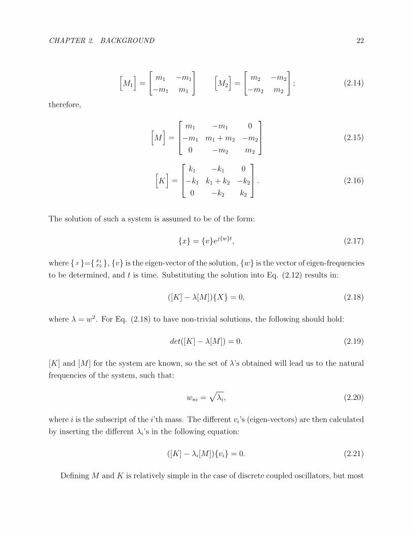
CHAPTER 2. BACKGROUND 22
hM1
i=
"m1 �m1
�m1 m1
# hM2
i=
"m2 �m2
�m2 m2
#; (2.14)
therefore,
hM
i=
2
64m1 �m1 0
�m1 m1 +m2 �m2
0 �m2 m2
3
75 (2.15)
hK
i=
2
64k1 �k1 0
�k1 k1 + k2 �k2
0 �k2 k2
3
75 . (2.16)
The solution of such a system is assumed to be of the form:
{x} = {v}ej{w}t, (2.17)
where { x }={ x1x2 }, {v} is the eigen-vector of the solution, {w} is the vector of eigen-frequencies
to be determined, and t is time. Substituting the solution into Eq. (2.12) results in:
([K]� �[M ]){X} = 0, (2.18)
where � = w
2. For Eq. (2.18) to have non-trivial solutions, the following should hold:
det([K]� �[M ]) = 0. (2.19)
[K] and [M ] for the system are known, so the set of �’s obtained will lead us to the natural
frequencies of the system, such that:
w
ni
=p�
i
, (2.20)
where i is the subscript of the i’th mass. The di↵erent vi
’s (eigen-vectors) are then calculated
by inserting the di↵erent �i
’s in the following equation:
([K]� �
i
[M ]){vi
} = 0. (2.21)
Defining M and K is relatively simple in the case of discrete coupled oscillators, but most
CHAPTER 2. BACKGROUND 23
of the systems we deal with in reality are continuous structures, rather than discrete sets of
oscillators. It is possible to simplify and approximate linear continuous structures as sets of
coupled harmonic oscillators, whose equations of motion determine the approximate dynamic
behaviour of the structure as a whole. To be able to analytically determine the natural
frequencies and eigen-modes (eigen-vectors) of a linear continuous structure, however, the
structure must be simplified to a great extent, and this simplification must take into account
the Degrees of Freedom (DOF) that are most significant in determining the vibrational and
dynamic behaviour of the structure. Degrees of Freedom in this case refer to the masses
whose dynamic motions are described by the EOM. The more accurate this approximation
is, the more di�cult it would be to determine the solution to the di↵erential equations
analytically.
In his book, The Science of String Instruments, Rossing states that at low frequencies,
the soundboard, the enclosed air and the back plate contribute to the sound radiation of the
instrument, but at higher frequencies, most of the sound is radiated by the soundboard [1,
p. 20]. A 2-DOF representation of the acoustic guitar was first proposed by Caldersmith
in 1978 [41], where the ribs and the back plate of the instrument are assumed fixed, while
the soundboard and the enclosed air are regarded as the two DOF determining the dynamic
behaviour of the instrument. In this model, presented in Fig. 2.15, [K] would be defined
in terms of the elastic properties of the soundboard and the enclosed air. It is therefore
understandable that the volume and the properties of the air inside the sound box will play
a role in the modal characteristics of the instrument model, as would the geometric, physical
and material properties of the soundboard.
Figure 2.15: (a) The 2DOF guitar model, (b) Frequency response of a Martin D-28 with itsbackplate and ribs fixed in sand [1, p. 26].
Later, a 3DOF model of the guitar was proposed by Christensen [42], taking the back
CHAPTER 2. BACKGROUND 24
plate into account, and a 4DOF model proposed by John Popp [43], with the ribs added to
the model. As you can notice, the common components present in all these models are the
soundboard and the enclosed air. Since the harmonics present in the sound of the guitar in
a large range of frequencies are generated by the soundboard, the behaviour of the guitar, to
a first approximation, is thought to be dominated by the behaviour of the soundboard. This
is why the soundboard was chosen as the first component of the instrument that is made
from alternative materials and monitored through this design and material replacement.
2.4.2 The Finite Element Method
While simplified mathematical models are a good starting point for modelling instruments, a
much larger set of di↵erential equations is required to accurately model a complex structure
like the guitar. The more complex the structure, the more analytical equations are required
to describe the behaviour of a structure, and the more di�cult it is to analytically solve
them. It is in fact not practical to represent such complex structures analytically and to
look for exact analytical solutions to these equations. In such cases, engineers use the Finite
Element Method (FEM) to discretize the structure, and numerically determine the static or
dynamic behaviour of the structure under di↵erent circumstances.
Figure 2.16: Some common element types used in FEM [44]. 1st line: linear elements. 2ndline: quadratic elements.
In every FEM representation, the structure is approximated using a large but finite set
of elements. The elements can be 1D, 2D or 3D, and can be linear, quadratic, cubic, etc.
CHAPTER 2. BACKGROUND 25
Depending on the dimension and the order of the elements, each element will consist of a
limited number of nodes. The solution to the di↵erential equation is computed at nodes and
interpolated between them. Interpolation is done by functions referred to as shape function,
N
i
. Shape functions are usually polynomials of some order n, and essentially act as weights
on the nodal solutions, making the solution for every element of the form:
u(x) ⇡ N1(x)u1 +N2(x)u2 +N3(x)u3 + ...+N
n
(x)un
=nX
i=1
N
i
(x)ui
, (2.22)
where n is the order of the element (not its dimension), i is the node subscript, x is the
independent global variable, and u(x) is the parameter of interest, i.e. the solution to the
di↵erential equation at x. Therefore although the solution is computed for a discrete set of
points, with the help of shape function, it can be computed for the continuous domain of
x within every element. Fig. 2.16 is an example of the solution - in this case temperature
profile - being represented using two quadratic 1D elements.
Figure 2.17: Temperature profile represented across two quadratic elements [44].
Once the structure is discretized, the K and the M for every element j will be defined
as:
[Mj
] =
ZZZ
V
[Ni
]⇢[Nj
]T �V (2.23)
[Kj
] =
ZZZ
V
[Bj
]TEj
[Bj
]�V, (2.24)
CHAPTER 2. BACKGROUND 26
where [Bj
]= �
�x
[Nj
], and E
j
is the elasticity matrix of the element, in compliance5 form. For
an orthotropic material, like wood, Ej
of its elements would be described as:
[Ej
] =
2
6666666664
1E
x
�v
yx
E
y
�v
zx
E
z
0 0 0�v
xy
E
x
� 1E
y
�v
zy
E
z
0 0 0�v
xz
E
x
�v
yz
E
y
� 1E
z
0 0 0
0 0 0 12G
yz
0 0
0 0 0 0 12G
zx
0
0 0 0 0 0 12G
xy
3
7777777775
. (2.25)
GivenM andK for every element, the eigen-frequencies and eigen-vectors can be determined
for the system of elements, as described in Sec. 2.4.1.
2.4.3 Experimental Modal Analysis
Experimental modal analysis is the process of determining the dynamic properties of a
structure experimentally. While there are di↵erent possible forms of dynamic loads that
can be applied to a structure, the two useful forms of loading which can reveal important
information about the structure are applied using a shaker or an impact hammer. The
shaker test provides information on the response of the structure to cyclic loading only
at the frequency of the input, while the impact hammer test provides information on the
response of the structure at a large range of frequencies. The impact hammer test is useful
when the natural frequencies of the structure are unknown.
The method used in this project is the impact test, which consists of applying a single
impulse to the structure with a hammer-shaped force transducer in the direction normal
to the deflecting surface, while simultaneously measuring the response at another location
on the structure. The ratio of the measured response to the input force is considered,
and the Fourier Transform of this ratio is what is referred to as the Frequency Response
Function (FRF). The resulting FRF will be a complex function which carries magnitude
and phase information. The response parameters that can be measured are the velocity and
acceleration, and the FRFs corresponding to these measurements are respectively referred
to as mobility (admittance), and accelerance. It is worth noting that these functions are
algebraically related, and measuring one allows calculation of the other two. The FRFs used
in this thesis were mobility FRFs, calculated as follows:
5Hooke’s law in compliance form is [✏] = [C][�], where [C] is the sti↵ness in compliance form.
CHAPTER 2. BACKGROUND 27
Normalizing the EOM of a damped 1DOF oscillator, Eq. (2.12), results in
x+ 2⇣w0x+ w
20x =
F
m
, (2.26)
where w0 =q
k
m
, and ⇣ is the damping ratio of the oscillator. From this point, the mobility
function of the oscillator will be:
V (w)
F (w)= [
1
k
][jww
20
w
20 � w
2 + j(2⇣ww0)], (2.27)
where w is the frequency of excitation, and the magnitude and the phase expressions are,
respectively:
|V (w)
F (w)| = [
1
k
][ww
20p
(w20 � w
2)2 + (2⇣ww0)2] (2.28)
and
✓ = arctan(�w
20 + w
2
2⇣w0). (2.29)
As long as the impact location and the measurement point are not located on the nodes of
any mode, one perfect impulse would be adequate to reveal most of the natural frequencies of
the structure. However, for the mode-shapes to be known, it is required that the response is
measured at a set of pre-selected locations across the structure, while the impact location is
kept constant, or the other way around. This would create a map of the whole structure that
determines the vibrational behaviour of the structure at a large range of frequencies. [39]
Ideally, this is done under free boundary conditions, but in reality it is not possible to do so,
so the structure is set up such that there are minimal constraints applied to the structure
and the boundaries.
In the past, mode shapes were determined using Chladni’s method [45], and more recently
using holographic interferometry [46], or visualized using modal analysis software. The
response data can be obtained using an accelerometer or a Laser Doppler Vibrometer (LDV).
The input and the response data are then sent from the force transducer and the measurement
instruments to a Data Acquisition unit (DAQ), on to the software where the set of FRFs
obtained are assigned to the di↵erent selected points, and the mode shapes are visualized.
The visualization is done by making use of the real (i.e. magnitude) and the imaginary
parts (i.e. phase information) of the measured FRFs, and the dynamic property extraction
is done by curve fitting. Further procedural details on the experimental modal analysis will
be discussed in the methodology chapter.
CHAPTER 2. BACKGROUND 28
2.5 Literature Review: Determining the Quality of a
Soundboard
Over the past several decades, a considerable amount of research has gone into identifying the
factors that a↵ect the acoustical properties of materials, the extent of their e↵ects, and the
parameters that determine the quality of string instruments. Though the larger portion of
these studies is not specifically on guitars, the relationships between mechanical properties
and acoustical properties of soundboards hold for all acoustic string instruments such as
violins and guitars. The range of mechanical and acoustical properties that make the timbre
of the instrument more desirable, however, di↵er depending on the instrument. The following
review of the literature will list the mechanical properties that a↵ect acoustical properties
of guitar soundboards in particular.
Wood is the most widely used material for soundboard construction, but what makes
certain woods better candidates for soundboards? And what determines if other materials
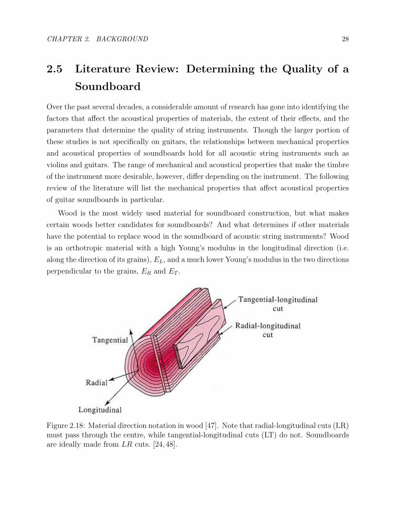
have the potential to replace wood in the soundboard of acoustic string instruments? Wood
is an orthotropic material with a high Young’s modulus in the longitudinal direction (i.e.
along the direction of its grains), EL
, and a much lower Young’s modulus in the two directions
perpendicular to the grains, ER
and E
T
.
Figure 2.18: Material direction notation in wood [47]. Note that radial-longitudinal cuts (LR)must pass through the centre, while tangential-longitudinal cuts (LT) do not. Soundboardsare ideally made from LR cuts. [24, 48].
CHAPTER 2. BACKGROUND 29
In his paper on Frequency Response of Woods for Musical Instruments [24], Ono states that
the high anisotropy in wood is one of the factors that makes wood a good candidate for
use in soundboards. In this study, he experimentally evaluates various acoustical properties
of a number of boards made from di↵erent materials. The experiments consist of exciting
boards made from di↵erent materials, including some softwoods (e.g. sitka spruce) and some
hardwoods (e.g. maple), and recording the pressure changes caused by their vibration, using
a microphone. The result of his experiments showed that the qualities that make softwoods
suitable for soundboard construction are:
� High anisotropy, i.e. high E
L
/E
R
� High EL/⇢, where ⇢ is density
� Low ⇢
� Low internal friction in the L direction (Q�1L
), i.e. the vibratory energy lost in the
form of heat.
Ono’s study suggests that the response of the soundboard in the high frequency region is
associated with the high E
L
of the soundboard material, and the low frequency responses are
associated with its low E
R
. It is worth noting that although high anisotropy is a desirable
feature in the soundboard woods, the preferred ratio of this anisotropy is di↵erent for dif-
ferent string instruments. Upon collaborating with some guitar and violin luthiers, Charles
Besnainou had found that guitar luthiers prefer a E
L
/E
R
⇡ 20, while violin luthiers prefer
a ratio of ⇡ 10 [15].
Finally, Ono introduces (E/⇢
3)12 as an “easy measure” of quality in acoustic materials,
i.e. the higher this fraction, the better the quality of a soundboard. This fraction is later
on used by many researchers [35, 49] and referred to as the Acoustic Coe�cient or Sound
Radiation Coe�cient. Ono’s study also clarified that softwoods have a higher overall power
level, and the peaks in their frequency responses are further apart than in hardwoods.
Ono was not the only researcher to study the acoustical properties of woods. In his paper
titled as Wood for sound [35], Wegst starts o↵ by reminding us that many mechanical and
physical properties are correlated. For instance, Young’s modulii and shear modulii of wood
in both radial and longitudinal direction are correlated with density, ⇢. He then explains
that in selecting materials for acoustic instruments, the most important acoustical properties
that must be considered are as follows:
CHAPTER 2. BACKGROUND 30
Speed of Sound (c): Speed of sound is defined as
c =
sE
L
⇢
. (2.30)
It decreases as temperature or moisture content increase. It also decreases slightly as fre-
quency and amplitude of vibration increases. Higher values of c are desired for woods used
in the construction of acoustic instruments.
Characteristic Impedance (z): Characteristic impedance is defined as
z = c⇢ =pE
L
⇢. (2.31)
It characterizes the ratio of the energy that gets reflected back at the coupling of two media.
Impedance is most important when vibratory energy is being transmitted from one medium
to another, where the impedances di↵er. Note that the reciprocal of impedance is admittance,
and that in musical instruments, a low z is desirable, i.e. a high admittance.
Sound Radiation Coe�cient or Acoustic Coe�cient (R): This parameter de-
scribes the extent to which the instrument body gets damped due to sound radiation, and
is defined as
R =
sE
L
⇢
3. (2.32)
A large sound radiation coe�cient is desired.
Loss Coe�cient (⌘): It is a measure of the extent of vibratory energy that is dissipated
in form of internal friction. Unlike the previous properties, loss coe�cient is independent of
density and Young’s modulus, and is frequency dependent. It is defined as:
⌘ = 1/Q =�
⇡
= tan , (2.33)
where is the loss angle 6, � is the logarithmic decrement7, and Q is the quality factor.
Acoustic Conversion E�ciency (ACE): Quoting Barlow (1997), Wegst states that
if we wish to increase the average loudness of the instrument, the parameter that needs to
6A measure of the material damping in viscoelastic materials.7Natural logarithm of the ratio of the amplitudes of every two consecutive peaks of a motion in the time
domain.
CHAPTER 2. BACKGROUND 31
be maximized is the sound radiation coe�cient, but if we wish to increase the peak response
of a soundboard, what needs to be maximized is the ratio of the sound radiation coe�cient
to the loss coe�cient. In 2014, in a study done by Jalili on the acoustical properties of
FRPs [49], this ratio is referred to as the Acoustic Conversion E�ciency (ACE):
ACE = R
tan(�)
Finally, Wegst organizes di↵erent materials in terms of the above parameters by means
of graphical representations. Two of those important graphs are provided below.
Figure 2.19: Left: R vs. ⌘ for di↵erent materials. Right: c vs. ⇢. Notice soundboard woodsand CFRPs on the graphs. [35].
In addition to the findings presented on the acoustical properties of woods, there is a
fair amount of literature available on the vibrational behaviour of string instruments (e.g.
[26] [50], etc.). In a series of studies done on the vibrational behaviour of a classical guitar,
Elajabarrieta et al. [51–54] studied the evolution of modal parameters of the guitar, i.e.
resonance frequencies, admittance, quality factors and mode-shapes through the di↵erent
stages of consturction. The first study consisted of an experimental modal analysis on
the soundboard of the guitar, and it reported on the changes in modal parameters along its
construction phases. The succeeding studies made use of the FEM to model the soundboard,
the back, the enclosed air and the guitar as a whole. The ideas and the results presented in
these studies were taken into account in the design and analysis process of this project, and
will be further explained in the following chapters.
Chapter 3
Methodology
The specific goal in this project was to design and manufacture a composite soundboard
that would have similar natural frequencies to those of a reference wooden one under hinged
Boundary Conditions (BCs). Ideally, the two soundboards would have similar natural fre-
quencies, mode shapes and acoustical properties, but as a starting point, natural frequencies
were used as the primary determining factor in the design of the composite soundboard, while
the mode-shapes and modal-damping values were also being monitored. In addition to the
above goal, it was important that the soundboard designed fulfills a number of static func-
tional requirements, i.e., to have adequate strength to withstand the tension of the strings,
and to be light enough to vibrate in response to conventional strings.
The wooden soundboard was borrowed from a guitar luthier based in Montreal, Joel
Barbeau, who shared some of his knowledge with us and allowed us to perform experiments
on two nylon-string guitar soundboards he had built, one of which was used as the reference
for our design. The top plate of this soundboard was made from Picea Abies, and the braces
from Sitka Spruce.
In order to meet the above goals and functional requirements, the bending sti↵ness, mass
and the strength of the wooden top plate were first used as guidelines for an initial top
plate design. A number of materials were considered for potential use in the top plate and
the bracing sandwiches. Using the Finite Element Method (FEM), the e↵ect of varying
certain physical, geometric and elastic properties of the materials were then determined on
the natural frequencies and mode-shapes of the soundboard under free and hinged BCs. The
composite soundboard that was determined to have natural frequencies relatively similar to
those of the wooden soundboard under hinged BCs was then manufactured. For verification
purposes, experimental modal analysis was performed on the wooden and the composite
32
CHAPTER 3. METHODOLOGY 33
soundboards.
It is worth noting that the criteria of matching natural frequencies does not guarantee
similarity in acoustic properties, especially from a perceptual point of view, as the relative
amplitude and damping ratios of the modes a↵ects the timbre of the instrument to great
extent as well. Furthermore, in the higher frequency range, the frequency spacing between
the modes tends to decrease, causing interaction between the normal modes and also making
it di�cult for us to distinguish between them. The significance of the instruments’ natural
frequencies in their timbre, however, is well known and has been looked at by many scientists
in the study of the timbre of instruments. Moreover, the modes of an instrument and its
soundboard are some of the few parameters that can be determined and monitored prior
to construction, through numerical modelling. Matching the natural frequencies, therefore,
seemed to be a reasonable starting point in the realm of the use of synthetic materials in
musical instruments.
As explained in Sec. 2.4.1, since the harmonics present in the sound of a guitar in a large
range of frequencies are generated by the soundboard, the behaviour of the guitar, to a first
approximation, is thought to be dominated by the behaviour of the soundboard. This is
why the soundboard was chosen as the first component of the instrument that is made from
alternative materials and monitored through this design and material replacement.
This chapter will provide the description of the steps taken in the course of the project.
Keep in mind that most of the decisions made throughout the design process were based on
simulation results of the wooden and the composite top plates under free BCs, and those
of the wooden and the composite soundboards under free and hinged BCs, most of which
will be further elaborated in Chap. 4. Furthermore, in the methodology proposed, we must
understand that it is not always possible to taylor a material to have the optimum geometric,
physical and elastic properties we are interested in, as many of these properties are correlated
(e.g. density and Young’s modulus). The practical design, therefore, comes down to choosing
available materials that would result in the best possible solutions.
3.1 Experimental Modal Analysis - Wood
It was important to identify certain modal characteristics of the wooden soundboard exper-
imentally, in order to have a reference for the numerical model of the wooden soundboard,
and the design of the composite one. The experiments aimed to monitor the natural fre-
quencies, mode-shapes and modal damping values of the soundboard, and were performed in
CHAPTER 3. METHODOLOGY 34
the Computational Acoustic Modelling Laboratory (CAML) in the Music Technology suite
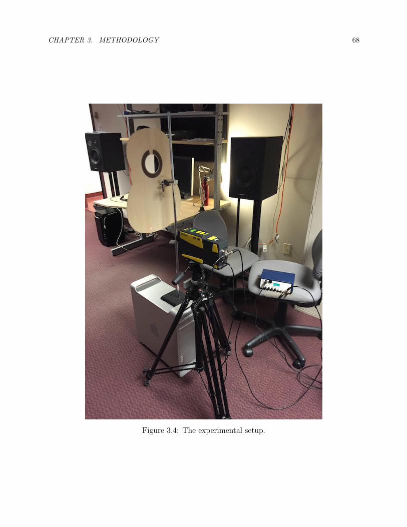
of the Schulich School of Music, McGill University. The experimental set up was as follows:
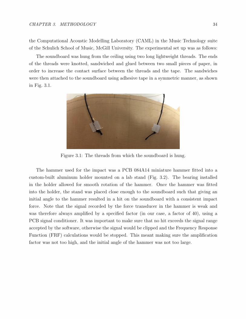
The soundboard was hung from the ceiling using two long lightweight threads. The ends
of the threads were knotted, sandwiched and glued between two small pieces of paper, in
order to increase the contact surface between the threads and the tape. The sandwiches
were then attached to the soundboard using adhesive tape in a symmetric manner, as shown
in Fig. 3.1.
Figure 3.1: The threads from which the soundboard is hung.
The hammer used for the impact was a PCB 084A14 miniature hammer fitted into a
custom-built aluminum holder mounted on a lab stand (Fig. 3.2). The bearing installed
in the holder allowed for smooth rotation of the hammer. Once the hammer was fitted
into the holder, the stand was placed close enough to the soundboard such that giving an
initial angle to the hammer resulted in a hit on the soundboard with a consistent impact
force. Note that the signal recorded by the force transducer in the hammer is weak and
was therefore always amplified by a specified factor (in our case, a factor of 40), using a
PCB signal conditioner. It was important to make sure that no hit exceeds the signal range
accepted by the software, otherwise the signal would be clipped and the Frequency Response
Function (FRF) calculations would be stopped. This meant making sure the amplification
factor was not too high, and the initial angle of the hammer was not too large.
CHAPTER 3. METHODOLOGY 35
Figure 3.2: The PCB 084A14 miniature hammer.
Ideally, the hammer must hit the soundboard only once, but due to the elasticity of
wood, a double-hit or multi-hit might be observed in the time-domain signal of the impact
hammer. Normally, one would monitor this and adjust the setup to minimize the e↵ect of a
double hit. That being said, the force signal is deconvolved from the measured velocity, so
the extra forces are taken into account in the input signal.
Figure 3.3: Example of a multi-hit time-domain signal from the hammer.
CHAPTER 3. METHODOLOGY 36
Mobility measurements were performed using an Polytec portable digital vibrometer LDV
(PDV 100). The laser was perpendicularly placed at a 23 cm distance from the soundboard
surface, as 23cm was listed as the shortest optimal stand-o↵ distance in the LDV manual.
For best results, the lens had to be adjusted until the focus of the laser was optimal.
In our experiments, the impact point was kept constant while the laser was moved from
one measurement point to another. A total of 41 points were selected as measurements
points. Note that we were not allowed to mark on the borrowed wooden soundboard, so the
locations of the impact point and the measurement points were marked on a paper cutout
of the soundboard instead. The cut out was attached to the soundboard using large paper
clips, and the hammer and the laser were placed based on the marks on the cutout. Once
the locations of the hammer and the laser were set, the cut out was removed. Every hit
was repeated 3 times, as the LDV measured the responses of the three hits. Between the
hits, we waited until the soundboard was stabilized before applying the next impact. The
average of the FRF’s obtained from the three hits were saved as the FRF corresponding to
that measurement point. Note that while performing the experiments, the relative humidity
of the laboratory was also monitored using a humidity sensor.
Both the hammer and the LDV signals, i.e. the input and the response signals respec-
tively, were sent to a National Instruments DAQ (PCI-4472). The DAQ transferred the
data to ME’scope, a software capable of analyzing and visualizing vibratory data. ME’scope
was used in our experiments to allow us to monitor the time-domain data received from the
hammer, the mobility FRFs, the modal damping values, the coherence between the averaged
signals, and to visualize the Operational Deflection Shapes (ODSs) at all frequencies.
Using BNC splitters, the input and the output signals were sent to a secondary digital
DAQ (USB-4431) that simultaneously sent the hammer and the LDV data to MATLAB.
This was done mainly in case we needed to access and process the raw time-domain data
later on, which is easier done on MATLAB. The MATLAB code developed for acquiring and
plotting the received data was written by Gary Scavone and Jim Woodhouse.
On ME’scope, the “frequency span” was set to 21,376.46 [Hz] 1, since the range of audible
frequencies for humans is 20,000 [Hz]. For adequate resolution of the FRFs, the number of
time-domain samples was set to 32768 per 0.766 seconds, so that it would result in 1.3 [Hz]
frequency increments, and the three FRFs corresponding to every measurement point were
averaged “linearly”.
1Note that this value is technically beyond the range the hammer practically captures, as it does notimpart significant energy above 9 kHz.
CHAPTER 3. METHODOLOGY 37
On ME’scope, a “structure” file, an “acquisition” file and a “BLK” file (referred to as
“data block”) were created. The structure was made up of the surface triangles connecting
the measurement points. The acquisition file was the platform through which the DAQ and
the software communicated, and where the di↵erent measurements were stored as “measure-
ment sets”. The data block was the file containing all the FRFs, coherences and the time
domain data. Note that other types of plots can be stored and analyzed in ME’scope as
well, e.g. correlation, but that the three mentioned were those we were interested in, in our
experiments.
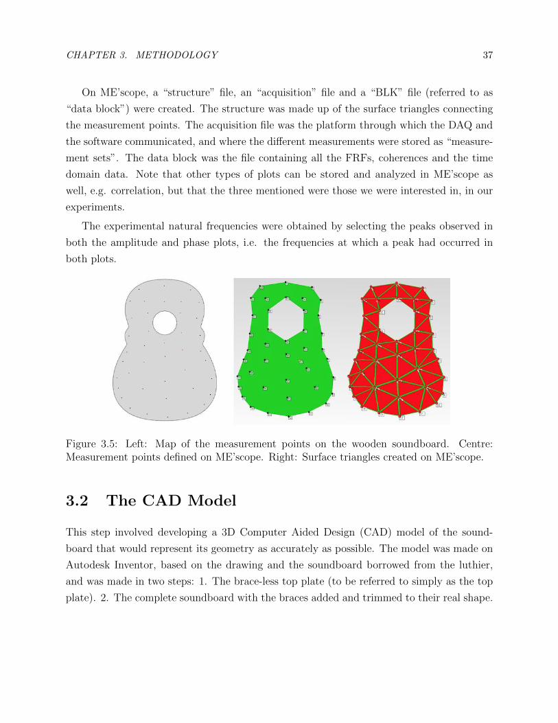
The experimental natural frequencies were obtained by selecting the peaks observed in
both the amplitude and phase plots, i.e. the frequencies at which a peak had occurred in
both plots.
Figure 3.5: Left: Map of the measurement points on the wooden soundboard. Centre:Measurement points defined on ME’scope. Right: Surface triangles created on ME’scope.
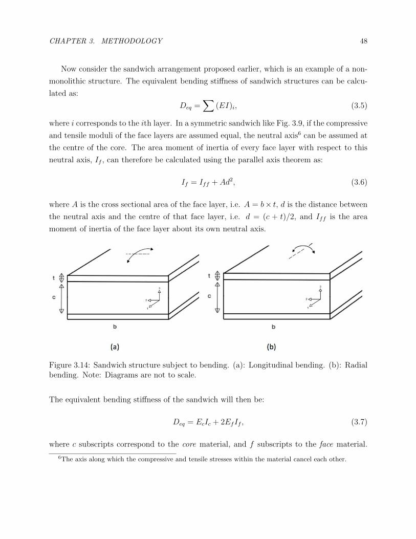
3.2 The CAD Model
This step involved developing a 3D Computer Aided Design (CAD) model of the sound-
board that would represent its geometry as accurately as possible. The model was made on
Autodesk Inventor, based on the drawing and the soundboard borrowed from the luthier,
and was made in two steps: 1. The brace-less top plate (to be referred to simply as the top
plate). 2. The complete soundboard with the braces added and trimmed to their real shape.
CHAPTER 3. METHODOLOGY 38
Figure 3.6: Left: the drawing of the soundboard. Centre: the braces behind the woodensoundboard. Right: The front side of the wooden soundboard. The top plate is made fromPicea Abie, and the braces from Sitka Spruce.
Figure 3.7: Left: The 3D CAD model of the wooden top plate. Right: The 3D CAD modelof the complete wooden soundboard.
CHAPTER 3. METHODOLOGY 39
3.3 Simulating the Modal Behaviour - Wood
The modal behaviour of the soundboard was determined using Abaqus CAE, a software
capable of performing Finite Element Analysis (FEA) 2. It features pre-processing (i.e. basic
CAD modelling), simulation, and post-processing (i.e. visualization and plotting) capabil-
ities. As explained earlier, the pre-processing was done on Autodesk Inventor, commonly
used for CAD modelling purposes, and the simulation and post-processing steps were per-
formed on Abaqus. The following tasks were performed once for the brace-less wooden top
plate, and once for the full wooden soundboard.
3.3.1 The Wooden Top Plate
1) Importing the Model: The CAD model of the top plate was imported from Inventor into
Abaqus as a 3D “part” in a .stp format.
2) Material Properties and Section Assignment: In the Property module, a material
directory had to be created in which certain properties of the materials used are defined. For
a frequency analysis, the density and the elastic properties of the material were required.
Picea Abies, as an orthotropic material, was therefore defined with its density and the 9
elastic constants listed in Table 3.1 (referred to as “Engineering Constants” on Abaqus).
Note that Abaqus does not require us to specify units for the values we enter, so it is
important to use a consistent system of units. The system used in our simulations is presented
in Table 3.2. For reference, the density and Young’s modulus of steel are listed. For other
possible systems of consistent units, refer to [55].
For the numerical model to implement the correct material anisotropy, material coordinates
must be defined. In case of assemblies, di↵erent coordinates must be defined for the di↵erent
constituent parts. In case of the top plate, however, only one material coordinate was
required. The top plate was then chosen as the section to which Picea Abies was assigned.
2Abaqus is also capable of performing Computational Fluid Dynamics (CFD), Computational Electro-magnetics and in general, Computer Aided Engineering (CAE).
CHAPTER 3. METHODOLOGY 40
Table 3.1: Density and Elastic Properties of Picea Abies and Sitka Spruce. S
b
, l and S
b
, r
are the longitudinal and the radial bending strengths. Values marked with * were given tous by the Luthier.
Properties Picea Abies Sitka Spruce
⇢* [kg/m3] 353 360
E1* [MPa] 10200 11880
E2* [MPa] 1020 927
E3 [MPa] 1600 927
⌫12 0.51 0.467
⌫13 0.38 0.372
⌫23 0.31 0.245
G12 [MPa] 754 724.68
G13 [MPa] 812 760.32
G23 [MPa] 36 35.64
Table 3.2: System of consistent units used. For reference, the density and Young’s modulusof steel are listed.
Mass Length Time Force Stress Energy Density Young’s Modulus Gravity
tonne mm s N MPa N-mm 7.83E-09 2.07E+05 9.81E+03
3) Assembly: To perform computation on a part or a set of parts, Abaqus requires us to define
an Instance. In this case, the whole top plate was chosen as an independent instance, in the
Assembly module.
4) Step: In the Step module, the type of analysis we wish to perform is specified, e.g. frequency,
heat transfer, etc., as well as the solution method and further specifications, e.g. frequency
range, increment size, etc. Our analysis was a frequency type for which we inquired all
the modes between 1-1000 Hz, and the eigen-solver was chosen to be Lanczos. Note that
the lower bound was specified in order to ignore the zero modes, and the upper bound was
CHAPTER 3. METHODOLOGY 41
roughly the highest fundamental pitch playable on a nylon-string guitar3. Since 32 modes
were obtained for the wooden soundboard in this range, all the following modal analyses on
the full composite soundboard was also concerning its first 32 modes.
5) Interaction, Constraints and Boundary Conditions: In the case of assemblies or
multiple parts in contact, the type of interaction the parts have must be defined, e.g. fixed,
surface-to-surface contact, etc. Di↵erent BCs can also be applied to the model, e.g. free-
translation fixed-rotation. In the modal analysis of the top plate, no BCs, constraints or
loads were required.
6) Mesh: In the Mesh module, the size, type and order of the elements of the numerical model
can be selected. The approximate global mesh size was chosen to be 3 with a maximum
0.1 deviation factor. The smaller the mesh size, the more accurate the results, but also, the
more time consuming the simulations can be. We found 3 to be su�ciently small. For a
more detailed explanation on selecting element size, refer to footnote 4.
7) Simulation: Every job created will contain the analysis results and field outputs requested in
the steps. If there are multiple steps defined in the step module, running the job will perform
all the computations requested and present all the results. Once the job is completed, it will
be possible to perform certain post-processings on the results, e.g. FRF plots.
8) Visualization of the Results: Once the Job is completed, the eigen-modes are reported
and the mode-shapes can be visualized.
3.3.2 The Wooden Soundboard
The soundboard assembly was imported into Abaqus as a single 3D part. It was introduced
as one independent assembly, and the above steps were performed on the full wooden sound-
board under free BCs. The eigen-frequencies and mode-shapes obtained from this simulation
were then compared to those obtained experimentally.
3One can argue that the higher partials of all notes are important, but the more important issue is thatthe modal density starts to get too high above 1-2 kHz for us to properly discern individual modes.
4In his article on discretization requirements [56], Marburg states that the minimum number of nodesrequired in acoustic computations of numerical models must go beyond fulfilling Shannon’s sampling theorem[57]. He believes that while adequate for wave “detection”, this number is not enough for approximating theshape of the elements, and he suggests a minimum of 6 to 10 nodes per wavelength of the highest frequencyof interest, i.e. equivalent to 3 to 5 linear elements.
CHAPTER 3. METHODOLOGY 42
In a series of studies done by Elajabarrieta et al. [51–54], it is stated that the bound-
ary conditions of a real soundboard attached to the ribs can be approximated as a fixed-
translation free-rotation boundary condition, referred to as “hinged” boundary conditions.
It was therefore decided to determine the natural frequencies of the soundboard under hinged
BCs as well. This required us to create a second job in which the new BCs were defined,
after having run the first job.
Figure 3.8: The numerical model of the soundboard is “hinged” along the final soundboardsilhouette.
Comparing Experimental and Numerical Mode-frequencies
In order to make correct comparisons between the numerical and the experimental results,
it was important to understand the di↵erence between how mode-frequencies are deter-
mined numerically, and how they are obtained experimentally. In the experiments, the
mode-frequencies were simply chosen by selecting the peaks that appeared in both the mag-
nitude plot and the imaginary plot of the mobility FRFs. The mode-frequencies reported
by Abaqus, however, are determined through computation of eigen-vectors and eigen-values
of the numerical model. Some of these eigen-vectors (or modes) might not have enough
amplitude to appear as “peaks” in the FRFs. This could be either because the excitation
point has happened to fall on a nodal point of those modes, or due to the uncertainties and
errors associated with the impact testing. Examples of these errors are those associated with
CHAPTER 3. METHODOLOGY 43
humidity or boundary conditions not accounted for.
Consider a mode-frequency vs. mode-number plot representing the experimental and the
numerical mode-frequencies (Fig. 3.9). With the above explanation, a correct comparison
between the two would be one in which the mode-frequencies obtained numerically are plotted
strictly sequentially, while those determined experimentally are not. In this case, every mode-
frequency from the experimental set would be compared with a numerical mode-frequency
in its vicinity. The point of the comparison would therefore be to observe whether for every
predicted eigen-frequency, a natural frequency is obtained experimentally, and if so, how
di↵erent are the experimental modes from the predicted modes, in terms of frequency and
mode-shape.
Figure 3.9: Graphical comparison of simulation and experimental natural frequencies. Left:Strictly sequential plotting. Right: Non-strictly sequential plotting. The yellow plot repre-sents the experimental natural frequencies, and blue represents eigen-frequencies obtainedthrough simulation.
3.4 Top Plate Simulation: From Wood to Composite
As explained earlier, every guitar soundboard must fulfill certain functional requirements.
It must have adequate strength to withstand the tension of the strings, and must be light
enough to vibrate in response to conventional strings. But aside from these requirements, in
this project, we were interested in making a composite soundboard whose natural frequencies
would also be similar to those of the reference wooden one.
CHAPTER 3. METHODOLOGY 44
Figure 3.10: The tension and moment caused by the strings [9].
We know that the natural frequencies of structures highly depend on their mass and
sti↵ness matrix, i.e., a function of E, G and ⌫ in the di↵erent directions. We are also aware
that according to the Euler beam theory, the natural frequencies of a free suspended beam
are related to its bending sti↵ness according to Eq. (3.1) [58], i.e.:
D
n
=Mw
2n
L
3
[(n+ 1/2)⇡ + k
n
]4, (3.1)
where D
n
is the bending sti↵ness, M and L are, respectively, the mass and the length of
the beam, wn
is the n’th natural frequency of the beam (in [rad/sec]), and k
n
is a mode-
dependent constant that can be found in [58, p. 64]. In more complex structures, however,
finding an analytical relationship between the bending sti↵ness and the natural frequencies
would not be as easy. Eq. (3.1) was, nevertheless, a hint for us to recognize a link between
natural frequencies and mechanical properties of a structure.
Furthermore, the mathematical relationships between vibrational frequencies and elastic
properties of simple structures, such as beams and pins, have long been used in optimization
problems and mechanical design techniques such as Ashby’s method [59]. In Ashby’s method,
the function of the structure is first defined, e.g. withstanding compression, or resisting
bending. Then considering the constraints (e.g. dimensional constrains), the function defined
allows us to find the optimal material properties for the structure, e.g. mass or cost.
When designing sandwich structures, however, with a vast range of potential materials
and their variability in properties, it may be more di�cult to treat the project as an “op-
timization” problem, especially considering the little research that has been done on the
use of composites in guitar soundboards, unless the potential materials are narrowed down
and many variables are treated as constraints, e.g. the thickness of the plate. Nonetheless,
CHAPTER 3. METHODOLOGY 45
Ashby’s approach and Eq. (3.1) led us to a meaningful starting point for our design process.
3.4.1 Why Sandwich Structures?
Sandwich structures have been used in many industries and applications in the recent
decades, due to their lightweight and high in-plane flexural sti↵ness [60]. In addition to
that, as mentioned in Chap. 2, their use has been explored in the literature of composite
guitars as well [6] [7] [8]. That, combined with the fact that producing sandwich structured-
composites manually is relatively easy, motivated us to explore the option.
3.4.2 Initial Proposition
To have a reference for our sandwich design, it was important to analyze certain mechanical
properties of the wooden top plate first. The top plate was approximated as a rectangular
plate made from Picea Abies, with the length, width and thickness of the wooden sound-
board, i.e. l = 490 [mm], b = 360[mm] and h = 2.3 [mm] respectively.
Figure 3.11: Left: the Inventor CAD model of the wooden top plate. Right: The rectangularapproximation of the wooden top plate, with length l = 490mm, width b = 360mm andthickness h = 2.3mm.
As a starting point, the materials available to us in the composites lab were considered
for use in a sandwich arrangement as depicted below. Among the available materials, it was
decided to consider the unidirectional composites for use in the sandwich structure, since
their anisotropy would be more similar to wood. Table 1 lists the uni-directional composites
CHAPTER 3. METHODOLOGY 46
that were available to us in the composites lab, as well as their required properties. In this
table, NCT321-UD (Unidirectional Newport 321) is made from uni-directional carbon fibres
pre-impregnated in epoxy resin, and was provided to us in form of pre-preg plies. Similarly,
Lineo FUD180 plies are made from pre-preg uni-directional flax fibres with epoxy resin [61].
Figure 3.12: The initial sandwich arrangement proposed for the top plate. Note that uni-directional fibres would be laid parallel to axis 1. Note: Diagram is not to scale.
Table 3.3: Elastic properties of the uni-directional materials considered. t is thickness andS
b,l
and S
b,r
are the longitudinal and radial bending strengths.
5Monolithic materials are made from two or more di↵erent materials, combined in such a way that theyare not easy to distinguish, so the combination is best treated as one single-phase material. [8]
CHAPTER 3. METHODOLOGY 48
Now consider the sandwich arrangement proposed earlier, which is an example of a non-
monolithic structure. The equivalent bending sti↵ness of sandwich structures can be calcu-
lated as:
D
eq
=X
(EI)i
, (3.5)
where i corresponds to the ith layer. In a symmetric sandwich like Fig. 3.9, if the compressive
and tensile moduli of the face layers are assumed equal, the neutral axis6 can be assumed at
the centre of the core. The area moment of inertia of every face layer with respect to this
neutral axis, If
, can therefore be calculated using the parallel axis theorem as:
I
f
= I
ff
+ Ad
2, (3.6)
where A is the cross sectional area of the face layer, i.e. A = b⇥ t, d is the distance between
the neutral axis and the centre of that face layer, i.e. d = (c + t)/2, and I
ff
is the area
moment of inertia of the face layer about its own neutral axis.
Figure 3.14: Sandwich structure subject to bending. (a): Longitudinal bending. (b): Radialbending. Note: Diagrams are not to scale.
The equivalent bending sti↵ness of the sandwich will then be:
D
eq
= E
c
I
c
+ 2Ef
I
f
, (3.7)
where c subscripts correspond to the core material, and f subscripts to the face material.
6The axis along which the compressive and tensile stresses within the material cancel each other.
CHAPTER 3. METHODOLOGY 49
Eq. (3.1) for longitudinal bending can then be written as:
D
eq,l
= E
c
bc
3
12+ E
f,l
[bt
3
6+
btd
2
2]. (3.8)
Since the Young’s moduli of foams are generally orders of magnitude smaller than those of
composites, the first term in Eq. (3.9) can essentially be ignored. The equation will therefore
be reduced to:
D
eq,l
⇠= E
f,l
[bt
3
6+
btd
2
2]. (3.9)
Similarly, the radial bending sti↵ness can be determined as:
D
eq,r
⇠= E
f,r
[lt
3
6+
ltd
2
2]. (3.10)
In the initial design, the total thickness of the sandwich was chosen to be that of the
wooden soundboard, and the face layers were chosen to be FUD180. Therefore t = 0.294
[mm], c = 1.712 [mm] and E
f
= 28200 [MPa]. Using Equations (3.9) and (3.10), the
longitudinal and radial bending sti↵nesses of the sandwich were calculated to be:
D
eq,l
⇠= 6.05⇥ 106[N.mm
2] and D
eq,r
⇠= 9.66⇥ 105[N.mm
2].
As explained earlier in the literature of guitar soundboards, a high longitudinal sti↵ness is
generally desired along the length of the soundboard. Based on that, the longitudinal bending
sti↵ness in these initial design calculations was used as the factor determining the similarity
between the wooden top plate and the composite one. Therefore given the longitudinal
bending sti↵ness obtained above, the bending sti↵ness of the sandwich rectangular plate
needed to be reduced. An easy way to reduce these values was to reduce the thickness of
the core foam. It was determined that with FUD180 as the face layers, a core thickness of
c = 1.275 [mm] would result in the same longitudinal bending sti↵ness as that of the wooden
plate, i.e.:
D
eq,l�FUD
⇠= 3.72⇥ 106[N.mm
2] and D
eq,r
⇠= 5.94⇥ 105[N.mm
2].
The other available material for face layers was the uni-directional Newport 321 with a
thickness of t = 0.16 [mm] and E
f
= 128242 [MPa]. The optimal foam thickness was found
to be c = 0.84 [mm] in this case, and the bending sti↵nesses as follows:
D
eq,l�NCT
⇠= 3.72⇥ 106[N.mm
2] and D
eq,r
⇠= 3.27⇥ 105[N.mm
2].
CHAPTER 3. METHODOLOGY 50
So far, with the above preliminary calculations, the thickness of the foam core was de-
termined for potential sandwiches with two di↵erent potential composite face layers. The
above results were to be regarded as a starting point for our simulations. We now had to
choose a foam whose physical and elastic properties would result in mode-frequencies similar
to those of the wooden top plate. This required us to start from an existing foam and vary
certain material properties of the core and the face layers, and to determine the e↵ects of
their variations on the mode-frequencies and mode-shapes of the top plate.
Note that in this process, it was not our intention to have the lightest possible soundboard,
but one that was light enough to be excited by conventional strings, while simultaneously
exhibiting similar mode-frequencies. The initial density of the core foam was therefore chosen
such that the thicknesses discussed would result in the sandwich top plate having the same
mass as the wooden one.
3.4.4 II. Using Simulation to Monitor the Eigen-frequencies
In Sec. 3.1.3, we simulated the modal behaviour of the wooden top plate and the wooden
soundboard. In this 2nd stage of the design, we simulated the modal behaviour of the
composite top plate as it was being designed.
The 3D CAD model of the top plate was imported into Abaqus as a 2D part. The com-
posite layers were introduced into the software as Lamina, and the foams were introduced
via Engineering Constants. For a frequency analysis, the density and 6 elastic constants
needed to be entered into the material directory, and material assignment was done using
composite layup. Under composite layup, the laminate materials were chosen from the ma-
terial directory, and were assigned to the layers in order. It was also in composite layup that
the thickness of every layer was entered, as well as their orientation.
The goal here was to simulate and monitor the eigen-frequencies of the proposed sand-
wiches, as the ⇢, E, G and ⌫ of the core and the face layers were varied, as well as the
thickness of the core. The boundary conditions at this stage were still free.
Foam Selection
The simulations started by exploring the foam options o↵ered by Evonik’s Rohacell foams,
since we had previously used their products and were aware of the wide range of material
properties they o↵er. In doing so, we had to keep the following in mind:
� The core foam must be able to withstand high curing temperatures of at least 121�C,
since FUD180 and NCT321 are cured at temperatures higher than that.
CHAPTER 3. METHODOLOGY 51
� The foam must be rigid, so it transfers vibratory energy between the composite layers.
This would also make sure that the foam doesn’t change shape under high vacuum pres-
sures during vacuum bagging.
� The foam must absorb enough resin to adhere to the pre-preg material in the curing
process. It should, however, not absorb too much resin to the extent that its properties
are a↵ected.
� The foam must be suitable for manually laying up pre-preg carbon fibres.
Properties Varied
After studying the properties of some existing composites and rigid foams, it was decided to
vary the specified material properties in the ranges practically available (Table 3.4).
Table 3.4: Range of the properties varied in the design of the top plate.
Throughout the calculations and the simulations, some of the potential sandwiches had core
foams of less than 1 [mm] thicknesses. Despite being theoretically optimal in some cases, after
an extensive search in the market, it was discovered that rigid foams are not commercially
produced in thicknesses of less than 1 mm.
To overcome this problem, it would have been possible to use spray foams instead, and
manually make the core foam with less than 1 [mm] thickness, but that would have required
a more complex moulding system which would make the manufacturing process more time
consuming and exhausting. The other option was to choose other core materials, such as
honey-comb Nomex which is already being used in double-top guitars. That idea was briefly
explored with the help of the honey-comb Abaqus plug-in, and while possible, modelling the
honey-comb layer was found to be highly time consuming.
CHAPTER 3. METHODOLOGY 52
With the issues stated, it was eventually decided to settle for higher than optimal thick-
nesses, and compensate for the excess sti↵ness of the top plate by making the braces less
sti↵.
The Modified Sandwich
After varying the properties stated and comparing the eigen-frequencies of the wooden top
plate with those of the composite top plate, it was decided to make the core from Rohacell
Rist 110 with a thickness of c = 1 [mm], and the face layers from one ply of uni-directional
NCT321 on each side of the foam.
Table 3.5: Properties of Rohacell Rist 110.
Material E1[MPa] E2[MPa] ⌫12 G12[GPa] G13[GPa] G23[GPa] ⇢ [kg/m3]
Rohacell Rist 110 180 180 0.3 70 70 70 110
3.4.5 III. Strength Criteria
Now that we had some idea about the arrangement of the top plate sandwich, it was time
to assess whether the sandwich proposed would have su�cient strength to withstand the
tension of the strings. The moment caused by the strings of the guitar were described by:
M
max,wood
=S
b
I
wood
y
, (3.11)
where Sb
is the bending strength of Picea Abies, and y is the distance from the neutral axis
to the location of maximum stress (i.e. the surface), hence y = h/2. Note that this equation
is applicable only to monolithic materials.
Most guitar soundboard woods are cured to have less than 12% moisture contents there-
fore the strength values for 12% were used in the calculations. Based on the longitudinal
and radial bending strengths listed in Table 3.6 (found in [62] and [63] respectively), the
maximum moment the rectangular wooden piece could withstand was then calculated as:
M
wood,l
= 75⇥360⇥2.32
6 = 23.81⇥ 103 [N.mm]
and
CHAPTER 3. METHODOLOGY 53
M
wood,r
= 6.4⇥490⇥2.32
6 = 2.76⇥ 103 [N.mm]
Table 3.6: Longitudinal and radial bending strength values of Picea Abies. Note that wherethe radial bending strength is marked with *, the moisture content of the Picea Abiesspecimen was listed as 10.5±0.5%, and not 12%.
Moisture Content [%] Sb,l
[MPa] Sb,r
[MPa]
12 75 6.4*
30 43 -
In sandwich structures, depending on the relative thickness and the relative sti↵ness of
the skin and the core layers, the structure can have di↵erent possible modes of failure. For a
sandwich structure with relatively thin and sti↵ skin layers and low core sti↵ness, the most
probable failure modes are failures due to face-sheet compression, or if the sti↵ness of the
core is too low, due to face-sheet wrinkling. [64, p. 209]
The maximum moment the composite sandwich experiences during compressive failure
Assuming that our rectangular approximation of the top plate is valid, the maximum
moments the wooden rectangular plate experiences at its highest stress in the longitudinal
and the radial directions are smaller than the moments the composite rectangular plate can
experience. Therefore, if the moment caused by the strings is applied to the composite top
plate, the composite top plate is not likely to fail due to facesheet compression:
M
max�comp,l
> M
max�wood,l
and M
max�comp,r
> M
max�wood,r
=) Composite rectangular
plate will not fail due to face-sheet compression.
CHAPTER 3. METHODOLOGY 54
On the other hand, the stress at which face-sheet wrinkling occurs can be determined by
Eq. (3.14) [64, p. 209]:
�
cr,l
⇠= c
3pE
f1Ec3Gc13 (3.13)
and
�
cr,r
⇠= c
3pE
f2Ec2Gc23, (3.14)
where c is a coe�cient between 0.5 and 0.8 determined experimentally, so:
�
cr,l
⇠= c
3p128242⇥ 180⇥ 70 = c⇥ 1173.46 [MPa]
and
�
cr,r
⇠= c
3p8274⇥ 180⇥ 70 = c⇥ 470.65 [MPa].
Since the sandwich is not built yet at this stage, the worst case scenario (i.e. if �cr,l
is
the smallest) was computed in the longitudinal and the radial directions as:
�
cr,l
⇠= 0.5⇥ 1173.46 = 586.73 [MPa].
and
�
cr,r
⇠= 0.5⇥ 470.65 = 235.33 [MPa].
Notice that the critical stresses at which the sandwich fails due to face-sheet wrinkling
in the longitudinal and radial directions are larger than the longitudinal and radial bending
strength of Picea Abies respectively (i.e. 75 [MPa] and 6.4 [MPa]). This means that the
allowable stress before face-sheet wrinkling occurs is su�ciently high, therefore face-sheet
wrinkling will not occur in the composite rectangular plate under the tension of the strings.
�
cr,l
> S
b�wood,l
and �cr,r
> S
b�wood,r
=) Composite rectangular plate will not fail due to
face-sheet wrinkling.
3.5 Adding the Braces - Simulation
The above results and considerations provided a starting point for the design of the complete
composite soundboard. It was now time to design the braces, in order to increase the eigen-
frequencies of the soundboard and match those of the wooden one. It is worth noting that
at this point, the design of the top plate sandwich was not considered finalized and could be
subject to change, if the simulation of the full soundboard suggested so.
CHAPTER 3. METHODOLOGY 55
Adding the braces to the composite top plate numerical model required us to have the
layout of the braces projected on the top plate plane. This was done by importing the 3D
CAD model as a 3D part, and creating partitions on one face of the top plate, by tracing
the bracing pattern. In Abaqus, 3D parts are visualized as empty 3D shells, and the faces
of the shell can be removed. When the bracing partitions were completed on one face of the
top plate, all the braces and the other faces of the soundboard were removed. The top plate
face with the partitions was then used as the base for the composite layup.
Just as was explained in Sec. 3.4, certain physical, geometric and elastic properties of the
constituent materials in the bracing sandwiches were varied in the simulations, while their
e↵ects on the eigen-frequencies of the soundboard were monitored. Note that the simulations
were first run with free boundary conditions, so we knew the inherent natural frequencies
of the soundboard, and then with hinged BCs. In both cases, the eigen-frequencies were
monitored up to 1000 Hz, and the mode-shapes up to the 10th mode.
Figure 3.15: Sandwich arrangement proposed for the braces.
The material properties were varied in a range similar to those listed in Table 3.4, but
larger foam thicknesses and other composite ply orientations were considered for use in
the bracing sandwiches. It was also noticed that using a sandwich arrangement with three
composite plies and two foam layers resulted in a better match of the eigen-frequencies (Fig.
3.14).
Based on to the simulation results that will be discussed in Chap. 4, Rohacell HF 71 was
found suitable for use in the bracing sandwiches, with the arrangements shown in Fig. 3.15.
The top plate sandwich remained as was decided in Sec. 3.4. Figures 3.16 and 3.17 show the
CHAPTER 3. METHODOLOGY 56
sandwich arrangements determined for the di↵erent parts of the soundboard.
Figure 3.16: Soundboard with the braces numbered.
Figure 3.17: Finalized sandwich arrangements. In the diagrams, grey corresponds toNCT321-UD, and white to foams. The foam used in all the braces is Rohacell HF 71,and the foam used in the top plate is Rohacell Rist 110. (a): The top plate sandwich. (b):Sandwich arrangement for braces 1 and 3. (c): Sandwich arrangement for braces 2, 4, 5, 6,7, 9, 10, 11, 12. (d): Sandwich arrangement for brace 8. Note: Diagrams are not to scale.
Table 3.7: Properties of Rohacell HF 71.
Material E1[MPa] E2[MPa] ⌫12 G12[GPa] G13[GPa] G23[GPa] ⇢ [kg/m3]
Rohacell HF 71 92 92 0.3 29 29 29 75
CHAPTER 3. METHODOLOGY 57
3.6 Construction
This stage consisted of laying up the sandwich layers in the planned order on top of a flat
aluminium mould, curing the sandwiches and finally, cutting them to the desired shapes.
The carbon fibre plies were available to us in form of large ply rolls at the Structures and
Composite Materials Laboratory, and the foams were delivered to us by Evonik Foams Inc. as
a courtesy to our research. The final materials used and their required properties are listed
below. Note that in Table 3.8, the Poisson’s ratios for the foams and NCT321 were not listed
in the data sheet of the products and were therefore selected to be 0.3 as a generic value
commonly reported for sti↵ foams and composites, based on a map adapted from Milton [65].
Table 3.8: Elastic properties of the materials analyzed.
Material E1[MPa] E2[MPa] E3[MPa] ⌫12 ⌫13 ⌫23 G12[MPa] G13[MPa] G23[MPa]
Table 3.9: Physical and geometric properties of the materials used.
Material Thickness [mm] ⇢ [kg/m3] Max. Temp. [�C]
Newport 321 0.16 1500 -
Rohacell Rist 110 1 110 180
Rohacell HF 71 4, 8, 10 75 ± 15 130
To work in the composites lab, all students are required to pass a Workplace Hazardous
Materials Information System (WHMIS) test first. They are also required to follow the
safety rules of the labs and have safety gloves and goggles on at all time, especially when
handling uncured pre-preg carbon fibres. In addition to goggles and safety gloves, however,
it is required to have face respirator and protective clothing on while performing dry or wet
cutting on carbon fibres.
CHAPTER 3. METHODOLOGY 58
3.6.1 Cleaning the Mould
The mould used for the top plate and the braces was essentially a rectangular aluminium
plate of 90 ⇥ 70 ⇥ 1 [cm3] dimensions. The mould surface was pre-sanded by the students
working in the composites lab, but to ensure carbon fibres do not stick to the mould, the
surface of the mould had to be cleaned with Zyvax mould cleaner, sealer and release agent
in order, according to their manuals. The mould was then used once in curing the top plate,
and once in curing the bracing sandwiches. Since the mould could accommodate all the
bracing sandwiches, they were all cured together.
3.6.2 Sandwich Layups
Both Rohacell Rist and Rohacell HF were stated to have low but satisfactory levels of resin
uptake, which ensures su�cient adhesion between the foam and the face layers, in this case
NCT321 [66] [67]. This means that as long as the core and the NCT321 layers are cured
together under the right amount of pressure, there will be no need for additional adhesives
to create a bond between the core and the NCT321 plies.
The clean mould was placed horizontally on a stable surface. The NCT321 and the
foam layers were then manually laid on top of one another on top of the clean mould in the
designed arrangements. It was important that the sandwiches were laid far from the edges of
the mould. Considering how much material was required for the braces overall, the bracing
materials (uncured pre-preg NCT321 sheets and Rohacell HF 71 foams) were initially cut
to large rectangles and placed in the desired arrangements. It was important to make the
rectangles bigger than we needed them to be, to leave enough margin for errors in cutting,
material that would fade away by the blade, and material that we needed to hold on to when
cutting the braces. The top plate materials, however, were cut out in a rough silhouette of
the guitar shape, slightly larger than needed. The sandwiches were to be cut to the correct
size later on, after being completely cured.
3.6.3 Vacuum Bagging
Vacuum bagging is the most common technique used for laminating sandwich-structured
composites. The process of vacuum bagging is as follows:
1) Place the mould horizontally on a stable surface and apply one row of sealant tape along
the edge of the mould, leaving 1-2 cm free margins outside the tape bounds. You should
CHAPTER 3. METHODOLOGY 59
end up with a rectangular tape running around the face of the mould. Do not remove the
top plastic cover of the tape yet.
2) Make sure the sandwich layups are placed inside the tape bounds, and that there is some
uncovered mould surface within the tape bounds, where the valve can be placed later on.
Note that once cured, the side of the sandwich that is in contact with the mould will have
a flatter surface.
3) Cut a piece of perforated release film and place it flat on top of all the parts. Make sure
the release film is large enough to cover all the parts, but not too large to overlap with the
sealant tape.
4) Cut a piece of breather and place it on top of the release film. Stay within the tape bounds.
5) Cut a large rectangular piece of vacuum bag. The piece must be a few inches larger that
the taped area.
6) Locate the lower part of the valve between the breather and the vacuum bag, not overlap-
ping the part. Place the vacuum bag on top of all the layers (including the sealant tape).
Remove the top plastic cover of the tape little by little, and start attaching the vacuum
bag from one corner. It is best if the vacuum bag is loose and not perfectly flat, so the bag
can deform without altering or damaging the sandwich, when the vacuum pump is turned
on. In order to avoid air passages forming between the tape and the vacuum bag, insert a
small ball of sealant tape in the gap between the bag and the tape, before removing the
last parts of the tape (Fig. 3.18).
7) Make a small cut in the vacuum bag, where the hole of the valve lies. Insert the upper part
of the valve inside the lower part (through the vacuum bag) and lock the valve.
CHAPTER 3. METHODOLOGY 60
Figure 3.18: The vacuum bag before attaching the vacuum pump. Notice the inserted ballof sealant tape on the right, and the valve at the top corner.
8) Attach a vacuum pump to the valve and observe as the air is removed from the bag. Watch
out for air gaps that make noises during vacuuming, and seal the gaps by applying pressure
on the sealant tape.
9) Remove the air pump and attach a pressure gauge to the valve. Observe the pressure gauge
for about half a minute. If the pressure value is stable, the bag has been sealed properly. If
not, look for possible air passages and block them by applying further pressure on the tape
or adding more tape to the sides. Apply vacuum and measure the pressure again. Repeat
until the bag is fully sealed.
3.6.4 The Curing Process
Once the vacuum bag was ready, it was placed in a 24 cu ft Blue M oven. The vacuum
pump was attached to the valve before closing the oven doors, in order to remove all air and
maintain the pressure desired for the mould throughout the cure cycle.
Newport 321 can be cured in temperatures between 121-149�C, depending on the time
spent at the peak cure temperature. Since Rohacell Rist and Rohacell HF could be handled
CHAPTER 3. METHODOLOGY 61
in temperatures of up to 180�C and 130�C, respectively, there was no need to worry about
their mechanical properties altering, as long as the sandwiches were cured at temperatures
below 130�C. To be on the safe side, however, it was decided to cure the sandwiches at the
minimum recommended cure temperature of 121�C.
While there was one specific cure cycle mentioned in the specifications sheet of NCT321,
there are other cure cycles that could be used to cure the NCT321 plies to the same degree-
of-cure. The cure cycle chosen was as shown in Fig. 3.19.
Figure 3.19: Ramp up from 25�C to 121�C in 1 hour (i.e. rate of 1.6�C/min), hold for 6hours, and cool down to 25�C in one hour.
CHAPTER 3. METHODOLOGY 62
Figure 3.20: Vacuum bags after the cure. Top: The vacuum bag containing the top plate.Bottom: The vacuum bag containing the bracing sandwiches. Notice that the silhouette ofthe top plate is slightly larger than the desired shape, and that it is yet to be trimmed.
CHAPTER 3. METHODOLOGY 63
3.6.5 The Cutting Process
The braces were cut out of the cured rectangular sandwich plates using a RUBI DX-350 wet
bridge saw. The saw was quite large and was not an optimal tool for cutting to such small
dimensions with little room for error, but since carbon dust is extremely invasive, it was
important that the parts were either cut in a specific dry-cutting booth, or are done through
wet cutting. Given the circumstances, it was decided the best tool available for straight
cutting was the wet bridge saw.
Figure 3.21: The wet bridge saw RUBI DX-350 [68].
The cured top plate on the other hand, could not be cut using the saw, and was manually
trimmed using a Dremel, i.e a rotary cutting and trimming tool. The Dremel was also used
to trim the edges of some of the braces to the exact angles and curves required. Note that
the Dremel, and in fact any other dry-cutting tool, had to be used in a designated space with
adequate ventilation power, to suck the carbon dust away. For that purpose, the designated
booth for dry-cutting carbon fibres was used, located in the Faculty of Engineering of McGill
university.
It is worth noting that we were aware of the fact that manually cutting the silhouette
of the soundboard was not an optimal technique. A better choice would have been to use a
water jet cutter to cut the top plate to the exact desired shape. It was decided not to pursue
this choice, however, simply due to lack of time and because it was not available to us on
campus.
CHAPTER 3. METHODOLOGY 64
Figure 3.22: The booth designated for dry cutting carbon fibres and composites.
Figure 3.23: Dry cutting the edge of the braces using the Dremel.
CHAPTER 3. METHODOLOGY 65
Figure 3.24: The manufactured composite top plate and the braces.
3.7 Experimental Modal Analysis - Composite Top Plate
In order to verify the eigen-frequencies and the mode-shapes obtained from the composite
simulations, it was required that an experimental modal analysis was performed on the
brace-less composite top plate, before attaching the braces. The procedure performed was
as explained in Sec. 3.1.1. One thing to take into account this time, however, was that the
side of the composite top plate that had been in contact with the mould now had a flatter
surface compared to the other side. The side that had been covered with the release film
was now more irregular, yet also very reflective, which could cause the laser to reflect faulty
phase data. We managed to notice this early on by monitoring the coherence of the response
signals, so we made sure the laser pointed to the flatter surface of the top plate. Note that
ignoring poor coherence could have resulted in faulty mode-shapes.
Figure 3.25: Close up shot of the two surfaces of the top plate. Left: The side facing thevacuum bag. Right: The side in contact with the aluminium mould.
CHAPTER 3. METHODOLOGY 66
After considering the first 10 mode-shapes of the soundboard (determined by the simu-
lation), the measurement points were selected with the intention to capture at least the first
10 mode-shapes and to not fall on their nodes7.
3.8 Attaching the Braces
The rougher side of the top plate was chosen as the front of the soundboard, simply for
aesthetic reasons, and the braces were attached to the composite top plate using Magnobond
56, an epoxy glue by Magnolia Plastics. The glue comes in a part A and part B that must
be mixed according to the MSDS of the glue. The cure time of the glue was stated to be
overnight in room temperature, though leaving the glue for longer would have resulted in
even stronger bonds.
Since the glue was not introduced in the numerical model of the soundboard, we did our
best to apply as little glue as possible, so that the final mass of the soundboard is not far
from that of the numerical model. We then left a number of heavy objects on the braces,
for better adhesion. The excess glue pushed out from under the braces was removed, and
the assembly was left to sit over night.
Figure 3.26: The braces were left under a number of heavy object over night for betteradhesion of the glue.
7Nodal points are the points that have zero displacement values in the mode-shapes.
Since the rougher side of the top plate was chosen as the front, the measurements had
to be taken from the back side of the soundboard, where the braces were attached. The
measurement points therefore had to be selected such that no point would fall on a brace or on
the nodal regions of the first 10 modes. Taking these into account, the experiments were done
as explained in Sec. 3.1.1. The natural frequencies and the mode-shapes of the composite
soundboard were then compared with those obtained from the composite simulation results
and will be discussed in the next chapter.
Figure 3.27: Left: Measurement points marked on the composite soundboard. Right: Themeasurement setup for the composite soundboard.
CHAPTER 3. METHODOLOGY 68
Figure 3.4: The experimental setup.
Chapter 4
Results and Discussion
4.1 The Wooden Soundboard
In this chapter, you will find the simulation and the experimental results obtained throughout
the design process. Keep in mind that in describing the results, mode-frequencies is the gen-
eral term used for the resonance frequencies obtained numerically and experimentally, natural
frequencies refer to the mode-frequencies obtained experimentally, and eigen-frequencies are
the mode-frequencies determined by the numerical model.
4.1.1 E↵ect of Environmental Factors
The first set of experiments on the wooden soundboard were performed in a span of 3 hours,
during which the natural frequencies were seen to shift by a 0-2 [Hz], depending on frequency.
To have an idea about the extent of these variations over time, the experiments were repeated
on two more days, the first two being 9 days apart, and the last two, 1 day.
Observing the Frequency Response Functions (FRFs) on di↵erent days revealed that
natural frequencies of a wooden structure like the soundboard can vary to large extents over
time. As shown in Fig. 4.1, the number and the frequency of the di↵erent peaks observed
in the FRFs are di↵erent on the first and the third day. This was believed to be due to the
variations of humidity and temperature over time.
Considering the frequency shifts of the modes over time, it was decided that the average of
the results obtained on the last two days were regarded as our reference. On the 2nd and the
3rd day of the experiments, the relative humidity and temperature values of the laboratory
were recorded, but their significance and their exact e↵ect on the natural frequencies remain
69
CHAPTER 4. RESULTS AND DISCUSSION 70
unknown, as it is not only the humidity and the temperature values at the time of the
experiments that a↵ect the natural frequencies, but more their variations over time.
Figure 4.1: FRFs representing the modal behaviour of the soundboard on the first and thelast day. The impact point and the measurement point corresponding to these FRFs werekept constant between the two day.
To quantify and better understand the extent of the changes in the FRFs over the days,
the natural frequencies and damping ratios of the first 10 modes were compared on the
di↵erent days. Figure 4.2 presents the frequency and damping values associated with the
modes observed on the 1st and the 3rd day. These parameters were extracted using the
curve fit and modal parameters features available in ME’scope, where the mode indicating
method was chosen as CMIF, and frequency and damping values were obtained using global
polynomial fitting 1. Notice the extent of variations in the natural frequencies and the
damping ratios on these two days.
To make sure the shift in the natural frequencies was not due to the the di↵erences
in the experimental set up on di↵erent days, the test was repeated with longer and shorter
1For more information on the di↵erent curve fitting options available in ME’scope, refer to [69].
CHAPTER 4. RESULTS AND DISCUSSION 71
threads and also with di↵erent attachment points on each day. It was observed that changing
the length of the threads or the attachment point of the threads did not a↵ect the natural
frequencies of the structure.
(a) (b)
Figure 4.2: Experimental natural frequencies and modal damping values of the woodensoundboard under free BCs. (a) Day 1. (b) Day 3.
4.1.2 Simulation vs. Experimental Results
The natural frequencies of the wooden soundboard obtained experimentally were compared
with the eigen-frequencies determined through simulation on a mode-by-mode basis, ac-
cording to the explanation provided in Sec. 3.3.2, i.e. the eigen-frequencies were plotted in
a strictly sequential manner, whereas the experimental natural frequencies were not. The
comparison (Fig. 4.3) showed a general agreement between the experimental and simulated
mode-frequencies in the range of 1-1000 [Hz], with the the exception of four modes missing
in the experimental results, and the central modes (13 to 18) appearing at lower frequencies
than expected. This is thought to be mostly caused by humidity and temperature varia-
tions. Table 4.1 lists the absolute di↵erences associated with every two mode-frequencies
being compared from the simulated and the experimental sets.
CHAPTER 4. RESULTS AND DISCUSSION 72
Figure 4.3: Experimental and simulated mode-frequencies of the wooden soundboard underfree BCs, plotted vs. mode number.
Next, the first 10 mode-shapes obtained numerically and experimentally were compared.
As shown in Fig. 4.4, the two sets were found to be in agreement. Note that the visual ac-
curacy of the experimental mode-shapes is a function of the number of measurement points
defined on the structure, and how the points are connected to one another using surface
triangles (Fig. 3.5). A finer representation of the mode-shapes would have required a higher
number of measurement points. In this case, the measurement points defined for the wooden
soundboard seemed su�cient for representing the first 10 mode-shapes.
CHAPTER 4. RESULTS AND DISCUSSION 73
Figure 4.4: Experimental and simulated mode-shapes of the wooden soundboard under freeBCs.
It is perhaps worth mentioning that the mode-shapes obtained for the wooden sound-
board were found to be quite comparable with the mode-shapes previously reported by
Elajabarrieta [51] [52], with the exception of modes 4 and 5 appearing in the opposite or-
der (Fig. 4.5). This could be due to the woods of the two soundboards being di↵erent,
the bracing patterns being di↵erent, and the fact that silhouette of the soundboard studied
CHAPTER 4. RESULTS AND DISCUSSION 74
in this thesis is slightly larger than its final intended shape. Furthermore, note that the
wooden soundboard studied in this thesis has 5 modes in the 0-200 [Hz] range, whereas the
soundboard studied by Elajabarrieta has 7.
Figure 4.5: The first 7 Experimental and simulated mode-shapes reported in [52].
CHAPTER 4. RESULTS AND DISCUSSION 75
4.2 The Top Plate: Simulation Results from Wood to
Composite
As part of the design process, the eigen-frequencies and the mode-shapes of the composite
top plate designed needed to be monitored and compared with those of the simulated brace-
less wooden top plate. In doing so, the e↵ect of varying the thickness, ⇢, E, G and ⌫ of
the core were monitored on the natural frequencies of the composite top plate, while the
available pre-preg composites were considered for use in the top plate sandwich.
FUD180
As explained in Sec. 3.4.3, a top plate made from FUD180 face layers and a 1.275 [mm] core
foam was first considered as a potential top plate layup. For the top plate to have a mass
equal to that of the wooden top plate, the foam (with a 1.275 [mm] thickness) would have
needed to have a ⇢ of about 25 [kg/m3]. However, among the lightest rigid foams o↵ered by
Rohacell, the lowest density was 32 [kg/m3]. This foam (Rohacell HF 31) was inserted in the
numerical model of the top plate as the core foam. The eigen-frequencies of this sandwich
layup are presented in Fig. 4.6.
Figure 4.6: Visualizing the e↵ect of varying the core thickness on eigen-frequencies of thetop plate, when the face layers are FUD180 and the core foam HF 31.
CHAPTER 4. RESULTS AND DISCUSSION 76
The eigen-frequencies of the mentioned composite top plate were found to be much lower
than those of the wooden top plate, which is why the modal behaviour of a sandwich top
plate with a higher core thickness (1.7 [mm]) was also simulated and presented. Notice that
an in crease in the thickness (and hence the sti↵ness) of the top plate results in an increase
in the slope of the Frequency vs. Mode Number curve. This means that as a result of
increasing the thickness of the core foam, higher eigen-frequencies are increased by a larger
amount, than the lower eigen-frequencies are.
Considering Ono’s comments about the e↵ect of G on higher eigen-frequencies [24], the
eigen-frequencies of the FUD/1.7mmHF31/FUD top plate being low in the higher modes
was believed to be due to the G of HF 31 being low. It was therefore of our interest to
better understand the e↵ect of varying the di↵erent properties of the core foam on the eigen-
frequencies. To do so, the E, G, ⌫ and the ⇢ of the HF 31 were varied to hypothetical values,
while the thickness of the core was kept constant, i.e., 1.7 [mm]. The original material
properties of the foams discussed in this chapter are presented below. Figure 4.7 then
presents the e↵ect of varying certain elastic properties of HF 31 to the hypothetical values
specified.
Table 4.1: Properties of the Foams Considered.
Material E1[MPa] E2[MPa] ⌫12 G12[GPa] G13[GPa] G23[GPa] ⇢ [kg/m3]
Rohacell HF 31 36 36 0.3 13 13 13 32
Rohacell HF 51 70 70 0.3 19 19 19 52
Rohacell HF 71 92 92 0.3 29 29 29 75
Rohacell Rist 51 75 75 0.3 24 24 24 52
Rohacell Rist 110 180 180 0.3 70 70 70 110
Rohacell IG 110 160 160 0.3 50 50 50 110
Rohacell Hero 150 124 124 0.3 75 75 75 150
Rohacell Hero 200 180 180 0.3 109 109 109 205
Rohacell SL 200 306 306 0.3 123 123 123 205
CHAPTER 4. RESULTS AND DISCUSSION 77
Figure 4.7: Visualizing the e↵ect of varying the elastic properties of the top plate core foam,when the core foam is a 1.7 [mm] HF 31, and the face layers are FUD180. Note that the foamsmarked with a star have the same elastic properties as those of HF 31, with the exceptionthat the property specified for each foam is changed to the hypothetical value specified. Theorange and the dark blue curves fall under the yellow curve.
As can be seen in Fig, 4.7, increasing the E of the core foam has had almost no e↵ect
on the eigen-frequencies of the top plate, which was expected for a sandwich structure with
high-sti↵ness face layers and low-sti↵ness core. This is while increasing the G has caused
the eigen-frequencies to increase, especially in the higher frequency region, which confirms
Ono’s statement on the matter. Changing the ⌫ of the foam from 0.34 to 0.4 has also had
no significant e↵ect on the eigen-frequencies of the top plate2.
As expected, it can be seen in Fig. 4.8 that when the elastic properties are kept constant,
increasing the density of HF 31 core foam from 32 [kg/m3] to a hypothetical value of 75
[kg/m3] will result in a decrease in the eigen-frequencies of the top plate. In reality, however,
an increase in the density of the foam is accompanied with an increase in the E and the G
of the foam. The eigen-frequencies of the top plate were therefore monitored when HF 71
was used as the core foam instead, which is an available foam with a density of 75 [kg/m3].
2The value of ⌫ for non-rubbery materials is usually in the range between 0.3 and 0.5 [65].
CHAPTER 4. RESULTS AND DISCUSSION 78
Figure 4.8: Visualizing the e↵ect of varying the density of the top plate core foam (HF 31)to a hypothetical value of 75 [kg/m3], compared to when the core foam is replaced with HF71 of the same thickness. HF 71 has slightly higher G and E values, compared to those ofHF 31.
Notice that the eigen-frequencies of the top plate with a HF 71 core foam are higher than
those of the hypothetical HF 31* rho75, which is believed to be due to the higher G of HF
71 (92 [MPa]), compared to that of HF 31 (13 [MPa]). To better match the eigen-frequencies
of the wooden top plate, a core foam with a slightly larger G was desired. Rohacell Rist 71
was therefore chosen as a candidate. The eigen-frequencies of the top plate with a 1.7 [mm]
Rohacell Rist 71 core foam are shown in Fig. 4.9, compared to those of the HF 71 top plate.
The masses of these top plates are also listed in Table 4.2.
CHAPTER 4. RESULTS AND DISCUSSION 79
Table 4.2: Masses of the FUD top plates considered.
Material Mass [g]
Wooden Top Plate 114.0
FUD/1.275 mm HF31/FUD 115.0
FUD/1.7 mm HF31/FUD 117.0
FUD/1.7 mm Rist71/FUD 127.0
One thing that must be pointed out is that considering the mentioned FUD top plate
layups, it was noticed that while the top plate with 1.7 [mm] Rist 71 core foam generally
matched the wooden top plate in eigen-frequencies, regardless of the core thickness or density,
the first eigen-frequency of these FUD top plates were found to be quite low compared to
that of the wooden top plate (25.96 [Hz]). This was one of the reasons why we were interested
in looking into the use of NCT321 as a potential composite layer in the top plate as well.
Figure 4.9: The e↵ect of replacing HF 71 with Rist 71 of the same thickness, but with aslightly larger G.
CHAPTER 4. RESULTS AND DISCUSSION 80
NCT321
Similar to the above analysis, the possibility of making the top plate from NCT321 face layers
was also analyzed. NCT321 pre-preg plies have higher sti↵ness and density values compared
to those of FUD180, but they come in smaller thicknesses. The optimum core thickness and
core properties would therefore be di↵erent from those obtained for the FUD180 top plate
sandwich.
As explained in Sec. 3.4.3, the core thickness considered for use in the NCT top plate
sandwich was 0.84 [mm]. For this sandwich to have a mass equal to that of the wooden top
plate, the foam had to have a density of 400 [kg/m3]. There were, however, a number of
problems associated with the stated thickness and density:
1. Among the rigid foams o↵ered by Rohacell, the heaviest foams have a density of 205
[kg/m3].
2. The foams available are not commercially available in thicknesses of less than 1 [mm].
3. The heaviest rigid foams o↵ered by Rohacell (e.g. SL 200 and Hero 200) do not come in
thicknesses of less than 6 [mm].
Despite the issues stated above, the e↵ect of varying the ⇢ to hypothetical values were still
monitored on the eigen-frequencies of the top plate. Considering the fact that the desired
density for a 0.84 [mm] core is 400 [kg/m3], the desired density for the core foam with a
thickness of 1 [mm] was determined to be 335 [kg/m3], which again, was higher than the
foams available to us. The eigen-frequencies of the top plates made from the heaviest 1 [mm]
foam cores available were therefore determined. Notice that the eigen-frequencies of these
top plates are all generally higher than those of the wooden top plate.
CHAPTER 4. RESULTS AND DISCUSSION 81
Figure 4.10: The eigen-frequencies of NCT top plates with foams of high density. In reality,these foams are not commercially available in thicknesses of below 6 [mm].
As explained earlier, none of the foams mentioned in Fig. 4.10 are available in 1 [mm]
thicknesses. For that reason, the foams that had relatively high density and were available in
1 [mm] thicknesses were considered next. The eigen-frequencies of the top plates containing
these foams are presented below.
CHAPTER 4. RESULTS AND DISCUSSION 82
Figure 4.11: Eigen-frequencies of NCT top plates with foams of high density available in 1[mm] thickness. Notice that in case of 1 [mm] core thickness top plates, the thickness of thecore is so small that a density change from 71 [kg/m3] to 110 [kg/m3] does not result in asignificant change in mass. Also note that SL 200 is only provided for reference, and that itis not available in thicknesses of < 6 [mm].
Following the comparison between the eigen-frequencies, the first 10 mode-shapes of the
suggested FUD top plate and an NCT top plate were compared with those of the wooden
top plate in Fig. 4.12. It is important to realize that neither the eigen-frequencies nor the
mode-shapes of the composite top plate being similar to those of the wooden top plate
guaranteed that the eigen-frequencies and the mode-shapes of the braced soundboard were
going to match after adding the braces.
By now, we had therefore come to realize that the choice had to be made between
using FUD180 with a 1.7 [mm] Rist 71 core foam, or using NCT321 with a 1 [mm] core
foam of relatively high density, i.e. 71-110 [kg/m3]. At this point, it seemed to us that
FUD/1.7mmRist71/FUD would be a better candidate, but upon adding the braces in the
simulations (in Sec. 4.3), it became clear to us that the braced soundboards including the
stated FUD top plate would have significantly lower eigen-frequencies compared to those of
the wooden soundboard.
CHAPTER 4. RESULTS AND DISCUSSION 83
Figure 4.12: The simulated mode-shapes for the wooden and composite top plates underfree BCs. Left: wood. Middle: NCT/1mmRist110/NCT. Right: FUD/1.7mmHF71/FUD
CHAPTER 4. RESULTS AND DISCUSSION 84
4.3 Addition of the Braces: Simulation Results
With the proposed top plates, the material properties and the thickness of the layers used
in the bracing sandwiches (Fig. 3.15) were varied in the available ranges. Upon adding
braces to the NCT top plates, the foams listed in Table 4.2 were considered and inserted
into the numerical model of the braces with thicknesses of 2-10 [mm]. The eigen-frequencies
of the potential soundboards with di↵erent bracing layups were compared under free and
hinged Boundary Conditions (BCs). The ultimate goal here was to come up with a set of
bracing sandwiches that would result in the hinged composite soundboard to have similar
eigen-frequencies to those of the hinged wooden soundboard.
Among the bracing layups considered, two sets of layups, referred to as C1 and CZ, were
found to give the hinged composite soundboard eigen-frequencies relatively similar to those of
the hinged wooden soundboard. Figure 4.13 presents the eigen-frequency vs. mode-number
plots for the wooden soundboard and the two mentioned composite soundboards under
free and hinged BCs. Figure 4.14 presents the top plate used in both of these composite
soundboards, and Figures 4.15 and 4.16 show the sandwich layups used in C1 and CZ,
respectively.
Figure 4.13: Eigen-Frequencies of two potential NCT soundboards and the wooden sound-board under free and hinged BCs, plotted vs. mode number.
CHAPTER 4. RESULTS AND DISCUSSION 85
Figure 4.14: The sandwich layup of the NCT top plate used in C1 and CZ. Note that thislayup is for the whole top plate, and not only the red area.
Figure 4.15: Layup diagram of C1. Note: diagram is not to scale.
CHAPTER 4. RESULTS AND DISCUSSION 86
Figure 4.16: Layup diagram of CZ. Note: diagram is not to scale.
In Fig. 4.13, notice that even though CZ appears to be a better match for the wooden
soundboard when compared under free BCs, C1 is seen to be a better candidate when com-
pared under hinged BCs. Since the soundboard under hinged BCs is a closer representation
of the soundboard attached to the instrument body, the similarity between the hinged com-
posite soundboard and the hinged wooden soundboard was used as the main design criteria.
Based on these results, the sandwich layup of C1 was therefore considered a reasonable
candidate for use with an NCT top plate for now. Note that in this case, CZ was simply
presented as a representative of the other possible sandwich layups that were considered.
One might question why some of the braces in C1 and CZ are not symmetric through
their thickness, and whether a symmetric layup would have resulted in a di↵erent set of
eigen-frequencies. The eigen-frequencies of C1 with a symmetric through-thickness layup
were found to be quite similar to those of C1. The only reason a non-symmetric layup
was selected was that initially a third potential sandwich layup was also considered for use,
in which brace 8 was made from a 3 layer sandwich, and it would have been easier if the
thickness of the lower foam of the overlapping braces was equal to the thickness of brace 8.
The foams ordered were chosen so that both C1 and CZ layups could be built, if desired.
C1 was later on selected as the layup set of choice.
FUD
Next, di↵erent bracing layups were considered for use with the proposed FUD top plate
(FUD/1.7mmRist71/FUD). Figure 4.17 presents the eigen-frequencies of the soundboard
with two di↵erent bracing layups used with the mentioned FUD top plate. Note that the
braces used in FZ1 were those of C1 introduced above, and the braces used in F22 are
presented in Fig. 4.18.
CHAPTER 4. RESULTS AND DISCUSSION 87
Figure 4.17: Eigen-frequencies of FZ1 and F22 compared to those of the wooden soundboard.
Figure 4.18: Layup diagram of F22. Note: diagram is not to scale.
It is curious that even using considerably thick braces, like those in F22, has not in-
creased the eigen-frequencies of the soundboard to the desired extent under hinged BCs.
To increase the eigen-frequencies of the soundboard containing the FUD top plate, many
bracing sandwiches were considered. Among these layups were some containing more than 3
composite plies, some containing significantly thicker foams, and some including only FUD,
CHAPTER 4. RESULTS AND DISCUSSION 88
only NCT or a combination of the two. Using more than 3 composite layers seemed to make
the structure too heavy, causing the eigen-frequencies to decrease even further, and using
significantly thicker foams seemed to have little e↵ect on the eigen-frequencies, as can be seen
in F22 of Fig. 4.17, regardless of the type of the composite layers used. By this point, we
were convinced that for the soundboard, made from an FUD top plate, to have reasonably
high eigen-frequencies under hinged BCs, the thickness of the top plate core foam would
need to be increased.
Based on the above observations, it was decided to make the composite soundboard
from an NCT top plate (NCT/1mmRist110/NCT) and C1 braces. It is worth noting that
replacing the Rist 110 core foam of the top plate with HF 71 or IG 110 would not have made
a significant di↵erence in the eigen-frequencies, and the only reason Rist 110 was chosen over
the other two was that one Rohacell Rist 110 was already available to us in the Structures
and Composite Materials Laboratory. The mass of this simulated composite soundboard
was determined to be 111 [g], which is lighter than that of the wooden soundboard (151 [g]).
The first 10 mode-shapes of the selected composite soundboard were then compared to
those of the wooden one under free and hinged BCs in Figures 4.19 and 4.20, respectively.
Notice the di↵erence in the mode-shapes of the wooden and the composite soundboards,
their order of appearance, and how the mode-shapes change upon being constrained by the
BCs.
CHAPTER 4. RESULTS AND DISCUSSION 89
Figure 4.19: Simulated mode-shapes of the wooden and the designed composite soundboardsunder free BCs. Left: wood. Right: composite.
CHAPTER 4. RESULTS AND DISCUSSION 90
Figure 4.20: Simulated mode-shapes of the wooden and the designed composite soundboardsunder hinged BCs. Left: wood. Right: composite.
CHAPTER 4. RESULTS AND DISCUSSION 91
4.4 The Composite Top Plate: Experimental Results
4.4.1 The Masses
According to Abaqus, the mass of the composite top plate was predicted to be 82.5 [g],
while that of the constructed top plate was measured to be 85.4 [g]. The thickness of the
constructed top plate was also measured to be 1.6 [mm], while it was expected to be 1.32
[mm], which was most probably due to the uncertainty in the thickness of the core foam.
The di↵erence observed in mass was therefore believed to be due the thickness of the core
foam being larger than assumed, and perhaps slightly due to cutting the outline of the top
plate slightly larger than the intended outline, when using the Dremel.
Table 4.3: Mass of the top plates: simulation vs. experimental.
Part Mass [g]
Wooden Top Plate (Simulation) 114.0
Composite Top Plate (Simulation) 82.5
Composite Top Plate (Constructed) 85.4
Notice that although as a starting point, the density of the foam was chosen such that
the top plate would have a mass equal to that of the wooden top plate, from then on, when
matching the mode-frequencies was chosen as the main goal, the mass of the wooden top
plate was solely considered an upper bound for the mass of the composite top plate.
4.4.2 The Modes
From the 32 eigen-frequencies predicted for the composite top plate with free BCs in the
0-740 [Hz] range, 30 modes appeared as peaks in the FRFs obtained experimentally. As
can be seen in Fig. 4.21, the experimental natural frequencies were seen to be similar to
the predicted eigen-frequencies in the lower frequency range, and they start to diverge from
the predicted values as frequency increases. This divergence could be due to the excess 0.28
[mm] thickness of the core foam. Table 4.5 presents the numerical and the experimental
mode-frequencies of the composite top plate, and their absolute di↵erences.
CHAPTER 4. RESULTS AND DISCUSSION 92
Figure 4.21: Experimental and simulated mode-frequencies of the composite top plate underfree BCs, plotted vs. mode number.
CHAPTER 4. RESULTS AND DISCUSSION 93
Table 4.4: Simulation and experimental mode-frequencies of the composite top plate.
Mode Number Simulation [Hz] Experimental [Hz] Absolute Di↵erence [Hz]
1 23.926 27.6 3.67
2 41.624 44.3 2.68
3 65.158 63.5 1.66
4 77.713 81.5 3.79
5 90.678 93.5 2.82
6 106.31 114 7.70
7 130.96 139 8.04
8 169.75 177 7.25
9 187.71 186 1.71
10 191.39 - -
11 202.16 212 9.84
12 243.5 248 4.5
13 271.16 283 11.84
14 294.19 308 13.81
15 294.63 316 21.37
16 315.36 330 14.64
17 357.79 373 15.21
18 358.79 381 22.21
19 419.46 422 2.54
20 423.28 - -
21 432.75 447 14.25
22 468.95 482 13.05
23 501.69 526 24.31
24 508.68 540 31.32
25 548.39 563 14.61
26 553.88 578 24.12
27 581.61 604 22.39
28 603.66 636 32.34
29 638.17 666 27.83
30 652.59 676 23.41
31 659.59 706 46.41
32 724.68 738 13.32
Note that in this case, it was rather easy to know which modes are missing in the
experimental results, because the experimental and the numerical curves were seen to follow
a similar trend. If the curves followed largely di↵erent trends, it would have been di�cult to
know which modes are missing and which modes must be paired and compared. Furthermore,
CHAPTER 4. RESULTS AND DISCUSSION 94
the experimental mode-shapes were seen to di↵er from those predicted by the simulation
beyond the 9th mode, or they were seen to appear in a di↵erent order, so the pairs being
compared do not necessarily correspond to the same mode-shapes. Fig. 4.21 is therefore
meant to show the spread of the natural-frequencies of the constructed top plate in the
frequency region displayed, compared to its numerical model. The modal density of the
constructed top plate in the 0-740 [Hz] range is therefore 30 modes, whereas the numerical
model of the composite top plate had predicted a modal density of 32 modes in this range.
Finally, Fig. 4.22 presents the first 10 mode-shapes of the composite soundboard deter-
mined by the simulation and obtained experimentally. We can see that the first 9 mode-
shapes obtained experimentally match those determine by the simulation. The 10th mode
having a di↵erent mode-shape could perhaps be expected, since its frequency was also missing
from the set of the experimental natural frequencies in Fig. 4.21.
CHAPTER 4. RESULTS AND DISCUSSION 95
Figure 4.22: Mode-shapes of the composite top plate under free BCs. Left: simulation.Right: experimental.
4.5 The Composite Soundboard: Experimental Results
In attaching the braces, one practical modification had been made in the bracing layup of the
soundboard. In the numerical model of the composite soundboard, a thickness of 0.32 [mm]
was removed from the base of braces 4, 5, 6, 10 and 11, in the areas where they overlapped
brace 8. This was for simplicity in the numerical model, so that the braces could be placed
on top of brace 8 without a gap between the braces and the top plate. In reality, however,
CHAPTER 4. RESULTS AND DISCUSSION 96
the overlapping areas were not removed, as we feared that creating 0.32mm-deep slots at the
base of the braces with the wet saw might damage the braces further than intended. Other
than that, these slots had to be created at precise angles in the braces, so that no extra parts
overlapped brace 8, and creating them at precise angles would have been rather di�cult.
In the process of making the braces with the wet saw, a large portion of the bracing
sandwiches was thrown away, due to the high uncertainty of the saw. Mistakes in cutting
the braces would have therefore required us to cure and cut more braces, or perhaps even
order more foams. It was due to the risks associated with making the slots as well as time
constraints that it was decided to not create the slots and directly attach the braces on top
of brace 8. The gaps between the braces and the top plate were therefore to be filled with
glue and pressure applied to the ends of the braces. Unfortunately, the e↵ect of not creating
these 0.32mm-deep slots could not be determined before construction, as it was not possible
to define a slanted gap between the composite layups on Abaqus. The result was therefore
yet to be determined experimentally.
4.5.1 The Masses
The simulated and the measured masses of the wooden and the composite soundboards are
presented in Table 4.6. In this table, notice that despite having tried to use as little glue as
possible, it was expected that the mass of the constructed soundboard would still be higher
than that predicted by Abaqus, even if the top plate and the braces were cut to the exact
intended size. This is simply because the glue used was not introduced in the numerical
model of the composite soundboard, and neither was its mass.
Table 4.5: The predicted and the measured mass of the wooden soundboard, the braces andthe composite soundboard.
Part Mass [g]
Wooden Soundboard (Simulated) 151.0
Wooden Soundboard (Existing) 152.0
Composite Soundboard (Simulated) 110.0
Composite Soundboard(Constructed) 121.6
Composite Braces (Simulated) 29.4
Composite Braces (Constructed) 32.7
CHAPTER 4. RESULTS AND DISCUSSION 97
Based on the values reported in Tables 4.5 and 4.6, the total mass of the glue used in
the soundboard was calculated as:
121.6� 85.4� 32.7 = 3.5 [g]
Figure 4.23: The excess glue observed at the points of attachment of the braces and the topplate.
4.5.2 The Modes
From the 32 modes predicted numerically for the composite soundboard (with free BCs)
in the range of 1-1000 [Hz], 29 appeared as peaks in the measured FRFs. The frequencies
of these modes were seen to di↵er from the predicted values by 1.5 to 48.63 [Hz] (avg. of
19.3 [Hz]), among which the lower frequencies showed larger di↵erences. The di↵erences
observed between the numerical and the experimental mode-frequencies, especially in the
low-frequency region, are thought to be due to (1) the thickness of the top plate being
larger than assumed. (2) the top plate silhouette being slightly larger than intended. (3) the
presence of the glue in the composite soundboard and its e↵ect on the total mass, mechanical
properties and the modal behaviour of the soundboard, and (4) the 0.32mm-deep slots not
having been created in braces 4, 5, 6, 10 and 11. Table 4.7 presents these numerical and
experimental mode-frequencies and their absolute di↵erences.
CHAPTER 4. RESULTS AND DISCUSSION 98
Figure 4.24: Experimental and simulated mode-frequencies of the composite soundboardunder free BCs, plotted vs. mode number.
CHAPTER 4. RESULTS AND DISCUSSION 99
Table 4.6: Simulation and experimental mode-frequencies of the composite composite sound-board.
Mode Number Simulation [Hz] Experimental [Hz] Absolute Di↵erence [Hz]
1 35.352 31.2 4.15
2 76.109 73.1 3.01
3 167.36 94.7 72.66
4 173.63 125 48.63
5 204.5 206 1.5
6 237.56 252 14.44
7 291.77 - -
8 327.77 327 0.77
9 359.68 368 8.32
10 391 378 13.00
11 420.16 400 20.16
12 442.88 447 4.12
13 490.53 477 13.53
14 498.96 482 16.96
15 581.68 529 52.68
16 597.65 585 12.65
17 615.05 627 11.95
18 644.1 650 5.9
19 668.6 688 19.4
20 680.06 - -
21 713.84 - -
22 757.36 747 10.36
23 758.65 780 21.35
24 806.26 804 2.26
25 851.14 871 19.86
26 920.12 924 3.88
27 961.95 956 5.95
28 1000.7 992 8.7
29 1013.8 1003 10.8
30 1034.6 1070 35.4
31 1100.6 1120 19.4
32 1105.5 1140 34.5
The mode-shapes and the modal damping ratios of the first 10 modes of the constructed
composite soundboard (with free BCs) are presented in Figures 4.25 and 4.26, respectively.
Notice that the first 6 experimental mode-shapes are found to match the predicted ones, and
CHAPTER 4. RESULTS AND DISCUSSION 100
modes 7 to 10 are seen to be similar with some local di↵erences in shape.
Figure 4.25: Experimental and simulated mode-shapes of the composite soundboard underfree BCs.
CHAPTER 4. RESULTS AND DISCUSSION 101
Figure 4.26: The experimental natural frequencies and the modal damping values for thefirst 10 modes of the constructed composite soundboard, obtained from ME’scope.
It must be pointed out that unlike the case seen in Sec. 4.4.2, despite a reasonable agree-
ment observed between the experimental and the predicted mode-shapes, the experimental
and the numerical frequency vs. mode-number curves of the composite soundboard (shown
in Fig. 4.24) were seen to follow rather di↵erent trends, especially in the lower frequency
region. This made it di�cult for us to know which modes were missing, and which modes
from the numerical set had to be compared with every experimental mode. It was only after
comparing the experimental mode-frequency trend of the constructed composite soundboard
with that of the wooden soundboard that a similarity was observed between the trends, al-
lowing us to decide which pairs had to be compared. Figure 4.27 presents the numerical and
the experimental mode-frequencies of the wooden and the composite soundboards. One in-
teresting observation in this comparison is that while the first five natural-frequencies of the
constructed composite soundboard were seen to di↵er from those predicted numerically, they
are found to be really similar to the first five mode-frequencies of the wooden soundboard
(both the existing soundboard and its numerical model).
CHAPTER 4. RESULTS AND DISCUSSION 102
Figure 4.27: Experimental natural frequencies of the wooden and the composite soundboardsunder free BCs, plotted vs. mode number. Notice that the orange curve is superimposed onthe grey and the yellow curves in the first 4 modes.
The FRFs obtained from a similar point on both soundboards are presented in Fig. 4.28.
Keep in mind that our aim when designing the composite soundboard was not to match
the natural frequencies at this stage, but rather to match them under hinged BCs, so the
di↵erences in the mode-frequencies were expected, and the FRFs are presented simply to
observe the mode-amplitudes and search for similarities.
CHAPTER 4. RESULTS AND DISCUSSION 103
Figure 4.28: FRFs corresponding to the wooden and the composite soundboard. The mea-surement point was identical between the two soundboards, as well as the impact points.
4.6 Sources of Error
Considering the discussions elaborated in this chapter, the following are some of the factors
that may have resulted in di↵erences between the experimental and the simulation results:
� The frequency and the occurrence of peaks in the experimental FRFs are both sensitive to
boundary conditions, the tapping and measurement locations, the resolution of the sensors
used and human errors while conducting the experiments. The very act of choosing FRF
peaks as experimental natural frequencies for a structure can therefore be subject to a
number of errors.
� Aside from the errors associated with the process of experimental modal analysis, perform-
ing the experiments on an unpolished wooden structure like the wooden soundboard was
seen to be subject to changes due to humidity and temperature variations. If the results of
the experiments on the first day were taken as the reference for the wooden soundboard,
the mode-frequencies would have di↵ered from those predicted by the model.
CHAPTER 4. RESULTS AND DISCUSSION 104
� Considering the variability observed in the material properties of Picea Abies reported in
di↵erent sources, the extent to which we can rely on the reported physical, geometric and
elastic properties of Picea Abies is still questionable. A more reliable way of determining
these properties would have been to extract them experimentally. The same applies to the
foams and the composite materials used.
� As explained earlier, the thickness of the foams being used in the soundboard (especially
that of the top plate) played a role in the experimental mode-frequencies being di↵erent
from those predicted by the numerical model. The silhouette of the top plate being slightly
larger than the intended outline could have also been a source of mismatch in mode-
frequencies and mode-shapes.
� The presence of the glue in the constructed composite soundboard, and the 0.32mm-deep
slots not having been created in the overlapping braces is believed to play a role in the
di↵erences observed between the experimental and the numerical mode-frequencies and
mode-shapes of the composite soundboard.
4.7 Limitations Faced
The following are some of the limitations faced throughout the course of this project:
� Our design process mostly relied on simulation results, and the experiments on the compos-
ite parts were only meant for comparison and verification purposes, rather than being used
as a part of the design process. This was simply because not all the potential materials
considered were at our disposal throughout the project.
One consequence of this limitation was that a number of parameters that could be extracted
experimentally and could also be considered in the design process had to be disregarded,
e.g., loss coe�cient and modal damping values, as it was not possible to determine them
numerically or analytically for a complex structure like the guitar, prior to construction.
Another consequence was that we could not foresee possible mismatches between the ex-
pected geometric, mechanical and physical properties, and those of the delivered parts, or
mismatches between the numerical model and the constructed parts.
� Although it is possible to create FRFs on Abaqus from the determined modal data, creating
an accurate FRF with correct modal damping values required us to have the modal damping
ratios for every determined mode. These damping ratios can be determined experimentally,
CHAPTER 4. RESULTS AND DISCUSSION 105
but not numerically prior to construction. It was therefore not possible to determine FRFs
with correct damping values on Abaqus.
� A closer look at the eigen-frequecies of the di↵erent introduced numerical models reveals
that some of the neighbouring eigen-frequencies are less than 1 Hz apart. This means that
if these modes appear as peaks in the measured FRFs, the interaction between the two
would not allow us to identify them as two separate peaks.
� Although a wooden soundboard was used as the reference for our design, if there are
certain acceptable degrees of dissimilarities between di↵erent wooden soundboards, we are
unaware of the extent of these variations in their natural frequencies and modal parameters.
Therefore, although the natural frequencies and the modal properties of the constructed
composite soundboard are slightly di↵erent from the reference wooden one, its natural
frequencies and modal parameters might still fall within the acceptable range of variations
of wooden soundboards. To know whether that is the case or not, we would have needed
to perform experimental modal analyses on a number of similar wooden soundboards with
the same bracing pattern, material and geometry.
� Comparing experimental mode-frequencies to the predicted mode-frequencies depended on
whether the frequency vs. mode-number plot trends were somewhat similar. In cases where
the trends were seen to di↵er to large extents, it was di�cult to know which modes had
to be compared, especially since the mode-shapes start to appear at di↵erent orders as
frequency increases, and comparing modes based on mode-shapes becomes an unreliable
method at high frequencies.
Chapter 5
Conclusions and Future Work
5.1 Conclusions
The aim of this project was to use the Finite Element Method (FEM) to design and manu-
facture the soundboard of a nylon-string guitar from sandwich-structured composites, with
reference to an existing wooden soundboard, and to evaluate the accuracy of the numeri-
cal models of the wooden soundboard, the brace-less composite top plate and the braced
composite soundboard by means of experimental modal analysis.
The modal behaviour of the existing wooden soundboard was first studied through ex-
perimental modal analysis, where the natural frequencies of the wooden soundboard were
obtained in the range of 0-1000 [Hz] under free Boundary Conditions (BCs), as well as its
first 10 mode-shapes and modal damping values. The 3D CAD model of the soundboard was
then built, followed by a numerical simulation of the modal behaviour of the soundboard.
The natural frequencies of the wooden soundboard obtained experimentally were found to
vary to large extents over time, which was believed to be due to the variations of temperature
and humidity.
The bending sti↵ness, mass and the strength of the wooden top plate were first used
as guidelines for an initial composite top plate design. Using FEM, the e↵ect of varying
certain physical, geometric and elastic properties of the materials used in the top plate were
determined on its natural frequencies under free BCs. The e↵ect of varying the bracing
materials was then determined on the mode-frequencies of the composite soundboard under
free and hinged BCs. The composite soundboard that was determined to have natural
frequencies relatively similar to those of the wooden soundboard under hinged BCs, and
could be built from commercially available materials was constructed. To verify the results
106
CHAPTER 5. CONCLUSIONS AND FUTURE WORK 107
predicted numerically, experimental modal analyses were performed on the composite top
plate and the composite soundboard under free BCs.
The composite soundboard constructed was made up of a top plate sandwich layup
containing pre-preg carbon fibre face layers (Newport 321 plies) and a Rohacell Rist 110
core foam (NCT321/1mmRist110/NCT321), and braces of di↵erent thicknesses containing
Newport 321 plies and Rohacell HF 71 core foams.
The experimental mode-frequencies of the constructed composite top plate were seen to
match those predicted numerically in the lower frequency range, slightly diverging from the
numerical values as frequency increases, while following a similar trend. In the first 9 modes,
the experimental and the numerical frequencies were seen to di↵er by 1.66 to 8.04 [Hz] from
the predicted eigen-frequencies (avg. of 4.37 [Hz] absolute di↵erence), which we consider a
successful match. The higher natural frequencies, however, were found to be further from
the predicted values, i.e. 2.54 to 46 [Hz] away from the predicted eigen-frequencies (avg.
of 19.20 [Hz] absolute di↵erence). This was believed to be due to the thickness of the top
plate core foam being slightly larger than previously assumed. The 10th and the 20th modes
predicted were not excited, therefore the modal density of the constructed top plate in the
range of 0-740 [Hz] was 30 modes, while the predicted value was 32. Furthurmore, among
the first 10 mode-shapes of the constructed composite top plate, the first 9 were found to
match the predicted shapes.
In analyzing the results of the experiments on the braced composite soundboard, the first
6 mode-shapes were found to match those predicted by the simulation, and modes 7 to 10
were found to be similar with some local di↵erences. The experimental mode-frequencies up
to 1200 [Hz] were found to di↵er from the predicted values by 0.77 to 52.68 [Hz] (avg. of
17.22 [Hz]), with the low and mid-frequency modes exhibiting more significant mismatches.
The numerical and the experimental frequency vs. mode-number curves in this case were
seen to follow less similar trends. Modes 7, 19 and 20 were not excited, making the modal
density of the top plate 29 over the 0-1200 [Hz] range, while the predicted value was 32.
Surprisingly, the first few experimental mode-frequencies of the constructed composite top
plate were seen to follow a more similar trend to that of the wooden soundboard, than to
that of the numerical model of the composite soundboard.
Overall, the agreement observed between the numerical and the experimental results were
considered satisfactory, the use of the FEM was found useful and reasonably accurate in the
design of a soundboard made from sandwich-structured composites, and the objectives of
the project were met.
CHAPTER 5. CONCLUSIONS AND FUTURE WORK 108
5.2 Future Work
Studying the modal parameters of a guitar soundboard only gives us a partial idea about
the timbre of the instrument, and as explained in Chap. 2, once the soundboard is attached
to the rest of the body, the interaction between the soundboard and the body through the
boundaries will change the modal parameters of the soundboard. In order to determine
the vibrational behaviour of the instrument as a whole, it would be required to attach the
soundboard to the body and repeat the experiments on a full instrument. The loss coe�cient
and the damping ratios associated with the di↵erent modes could also be monitored, in order
to better describe the vibrational behaviour of the soundboard. This could be followed with a
psychoacoustic analysis of the sound of the constructed instrument. In fact, a psychoacoustic
analysis on the instrument would ultimately be the point where we can determines whether
we have succeeded in imitating the wooden soundboard, and if not, in what terms and
to what extent the sound of the instrument is di↵erent from that of the reference wooden
instrument.
One further analysis that can be carried out in continuation of this study is a stress
analysis on the wooden and the composite soundboard using the Finite Element Method.
For that, the bridge and the saddle of the instrument would need to be included in the
numerical model of the soundboard, and the exact tension of the strings will need to be
known.
Another component that could add value to this research is the study of the e↵ect of
temperature and humidity variations on the modal parameters of wooden soundboards,
where the temperature and the humidity of the space the soundboard is stored and tested
in is controlled and monitored over time, as well as the initial moisture content of the wood
and the heat treatments it has gone through.
Although a number of studies have been done on the variation and categorization of
wooden guitars, e.g. [14], as explained in Sec. 4.7, one thing that remains unknown to us is
the extent of variations conventionally observed between the vibrational behaviour of wooden
nylon-string guitar soundboards. It would therefore be useful to perform experimental modal
analyses on a large number of wooden soundboards, in order to have an idea about the extent
of these variations.
It is worth mentioning that even though sandwich-structured composites with the pro-
posed layup may be a reasonable replacement for wood in the construction of nylon-string
guitar soundboards, it is highly possible that creating custom-made composites, as opposed
CHAPTER 5. CONCLUSIONS AND FUTURE WORK 109
to pre-preg plies, can give us the freedom to create parts with specifically designed density,
thickness and elastic properties.
Last but not least, an idea that is worth exploring is the use of the genetic algorithm and
machine learning techniques in coming up with an optimized design for the composite sound-
board. As mentioned in Sec. 3.4, this project was not treated as an optimization problem,
mainly because there were technically infinite possibilities that could be tested. The genetic
algorithm has only recently been used in material selection problems like ours, which is based
on multi-objective functions with infinite possible solutions. In the case of this project, the
genetic algorithm could come up with a large number of possible soundboard designs, and
depending on how we define our optimization criteria, machine learning techniques could be
used to choose the most promising designs.
Bibliography
[1] T. D. Rossing, Ed., Science of String Instruments. Springer, 2010, vol. New York.
[2] (2012, February) Vanishing tonewoods. Living On Earth. [Online]. Available: