101
Finite Element Modeling and Analysis CE 595: Course Part 2 Amit H. Varma

Finite Element Modeling and
Analysis
CE 595: Course Part 2
Amit H. Varma

Discussion of planar elements
• Constant Strain Triangle (CST) - easiest and simplest finite
element
� Displacement field in terms of generalized coordinates
� Resulting strain field is
� Strains do not vary within the element. Hence, the name
constant strain triangle (CST)
� Other elements are not so lucky.
� Can also be called linear triangle because displacement field is
linear in x and y - sides remain straight.

Constant Strain Triangle
• The strain field from the shape functions looks like:
� Where, xi and yi are nodal coordinates (i=1, 2, 3)
� xij = xi - xj and yij=yi - yj
� 2A is twice the area of the triangle, 2A = x21y31-x31y21
• Node numbering is arbitrary except that the sequence 123
must go clockwise around the element if A is to be positive.

Constant Strain Triangle
• Stiffness matrix for element k =BTEB tA
• The CST gives good results in regions of the FE model
where there is little strain gradient
� Otherwise it does not work well.If you use CST to model bending.
See the stress along the x-axis - it
should be zero.
The predictions of
deflection and stress are poor
Spurious shear stress when bent
Mesh refinement will help.

Linear Strain Triangle
• Changes the shape functions and results in quadratic
displacement distributions and linear strain distributions
within the element.

Linear Strain Triangle
• Will this element work better for the problem?

Example Problem
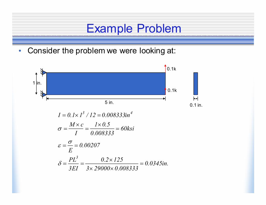
• Consider the problem we were looking at:
5 in.
1 in.
0.1 in.
I = 0.1×13 /12 = 0.008333 in4
σ =M × cI
=1× 0.50.008333
= 60 ksi
ε =σE
= 0.00207
δ =ML
2
2EI=
25
2× 29000×0.008333= 0.0517 in.
1k
1k

Bilinear Quadratic
• The Q4 element is a quadrilateral element that has four
nodes. In terms of generalized coordinates, its displacement
field is:

Bilinear Quadratic
• Shape functions and strain-displacement matrix

Bilinear Quadratic
• The element stiffness matrix is obtained the same way
• A big challenge with this element is that the displacement
field has a bilinear approximation, which means that the
strains vary linearly in the two directions. But, the linear variation does not change along the length of the element.
x, u
y, v
εxεx εx
εy
εy
εy
εx varies with y but not with x
εy varies with x but not with y

Bilinear Quadratic
• So, this element will struggle to model the behavior of a
beam with moment varying along the length.
� Inspite of the fact that it has linearly varying strains - it will
struggle to model when M varies along the length.
• Another big challenge with this element is that the
displacement functions force the edges to remain straight -no curving during deformation.

Bilinear Quadratic
• The sides of the element remain straight - as a result the
angle between the sides changes.
� Even for the case of pure bending, the element will develop a
change in angle between the sides - which corresponds to the
development of a spurious shear stress.
� The Q4 element will resist even pure bending by developing
both normal and shear stresses. This makes it too stiff in
bending.
• The element converges properly with mesh refinement and in most problems works better than the CST element.
Example Problem
• Consider the problem we were looking at:
5 in.
1 in.
0.1 in.
.in0345.0008333.0290003
1252.0
EI3
PL
00207.0E
ksi60008333.0
5.01
I
cM
in008333.012/11.0I
3
43
=×××
==
==
=×
=×
=
=×=
δ
σε
σ
0.1k
0.1k
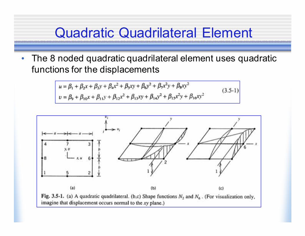
Quadratic Quadrilateral Element
• The 8 noded quadratic quadrilateral element uses quadratic
functions for the displacements

Quadratic Quadrilateral Element
• Shape function examples:
• Strain distribution within the element

Quadratic Quadrilateral Element
• Should we try to use this element to solve our problem?
• Or try fixing the Q4 element for our purposes.
� Hmm? tough choice.

Improved Bilinear Quadratic (Q6)
• The principal defect of the Q4 element is its overstiffness in
bending.
� For the situation shown below, you can use the strain
displacement relations, stress-strain relations, and stress
resultant equation to determine the relationship between M1
and M2
� M2 increases infinitely as the element aspect ratio (a/b)
becomes larger. This phenomenon is known as locking.
� It is recommended to not use the Q4 element with too large
aspect ratios - as it will have infinite stiffness
1 2
34
x
y
M1M2
a
b M2
=1
1+ υ1
1−υ+1
2
a
b
2
M
1

Improved bilinear quadratic (Q6)
• One approach is to fix the problem by making a simple
modification, which results in an element referred
sometimes as a Q6 element
� Its displacement functions for u and v contain six shape
functions instead of four.
� The displacement field is augmented by modes that describe
the state of constant curvature.
� Consider the modes associated with degrees of freedom g2
and g3.
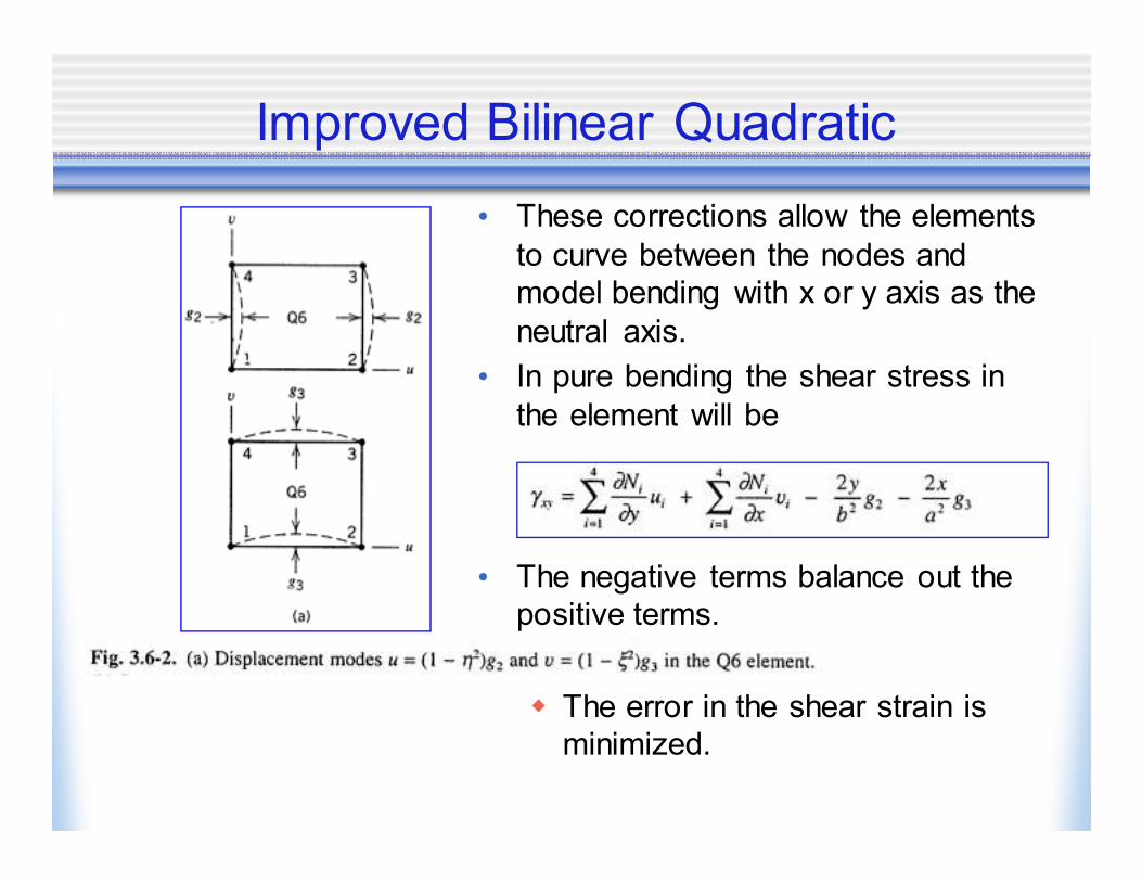
Improved Bilinear Quadratic
• These corrections allow the elements
to curve between the nodes and
model bending with x or y axis as the
neutral axis.
• In pure bending the shear stress in
the element will be
• The negative terms balance out the
positive terms.
� The error in the shear strain is
minimized.
Improved Bilinear Quadratic
• The additional degrees of freedom g1 - g4 are condensed
out before the element stiffness matrix is developed. Static
condensation is one of the ways.
� The element can model pure bending exactly, if it is
rectangular in shape.
� This element has become very popular and in many
softwares, they don’t even tell you that the Q4 element is
actually a modified (or tweaked) Q4 element that will work
better.
� Important to note that g1-g4 are internal degrees of freedom
and unlike nodal d.o.f. they are not connected to to other
elements.
� Modes associated with d.o.f. gi are incompatible or non-
conforming.

Improved bilinear quadratic
• Under some loading, on
overlap or gap may be
present between elements
� Not all but some loading
conditions this will happen.
� This is different from the
original Q4 element and is a
violation of physical
continuum laws.
� Then why is it acceptable?
Elements approach a state
Of cons

What happened here?
No numbers!

Discontinuity! Discontinuity!
Discontinuity!

Q6 or Q4 with incompatible modes
LST elements
Q8 elementsQ4 elements
Why is it stepped? Note the discontinuities
Why is it stepped?Small discontinuities?

Values are too low

Q6 or Q4 with incompatible modes
LST elements
Q8 elementsQ4 elements

Q6 or Q4 with incompatible modes
LST elements
Q8 elementsQ4 elements
Accurate shear stress? Discontinuities
Some issues!

BlackBlackBlack
Lets refine the Q8 model. Quadruple the numberof elements - replace 1 by 4 (keeping the same aspect ratio but finer mesh).
Fix the boundary conditions to include additional nodes as shownDefine boundary on the edge!
The contours look great!So, why is it over-predicting??
The principal stresses look greatIs there a problem here?
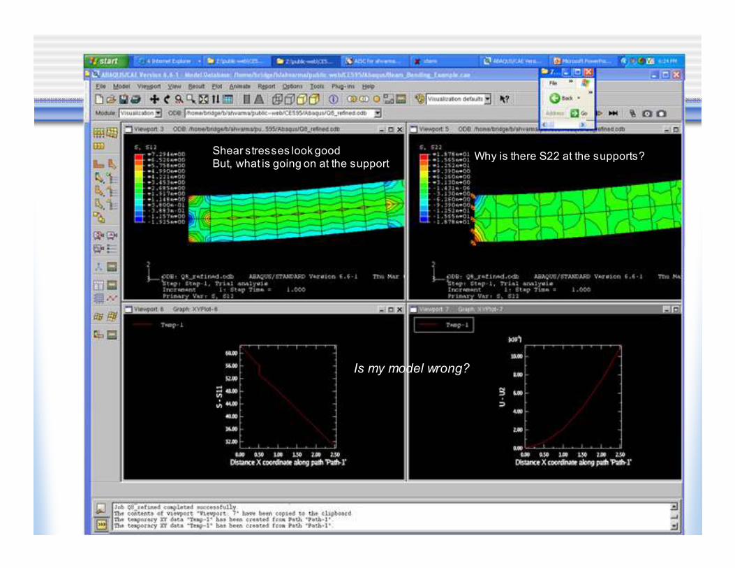
Shear stresses look goodBut, what is going on at the support
Why is there S22 at the supports?
Is my model wrong?

Reading assignment
• Section 3.8
• Figure 3.10-2 and associated text
• Mechanical loads consist of concentrated loads at nodes,
surface tractions, and body forces.
� Traction and body forces cannot be applied directly to the FE
model. Nodal loads can be applied.
� They must be converted to equivalent nodal loads. Consider
the case of plane stress with translational d.o.f at the nodes.
� A surface traction can act on boundaries of the FE mesh. Of
course, it can also be applied to the interior.

Equivalent Nodal Loads
• Traction has arbitrary orientation with respect to the
boundary but is usually expressed in terms of the
components normal and tangent to the boundary.

Principal of equivalent work
• The boundary tractions (and body forces) acting on the
element sides are converted into equivalent nodal loads.
� The work done by the nodal loads going through the nodal
displacements is equal to the work done by the the tractions (or
body forces) undergoing the side displacements

Body Forces
• Body force (weight) converted to equivalent nodal loads.
Interesting results for LST and Q8

Important Limitation
• These elements have displacement degrees of freedom
only. So what is wrong with the picture below?
Is this the way to fix it?

Stress Analysis
• Stress tensor
• If you consider two coordinate systems (xyz) and (XYZ) with the same origin
� The cosines of the angles between the coordinate axes (x,y,z)
and the axes (X, Y, Z) are as follows
� Each entry is the cosine of the angle between the coordinate
axes designated at the top of the column and to the left of the
row. (Example, l1=cos θxX, l2=cos θxY)
σxx
τxy
τxz
τ xy σ yy τ yz
τxz
τyz
σzz
x
y
z
X
Y
z
x y z
X l1 m1 n1
Y l2 m2 n2
Z l3 m3 n3

Stress Analysis
• The direction cosines follow the equations:
� For the row elements: li2+mi
2+ni2=1 for I=1..3
l1l2+m1m2+n1n2=0
l1l3+m1m3+n1n3=0
l3l2+m3m2+n3n2=0
� For the column elements: l12+l2
2+l32=1
Similarly, sum (mi2)=1 and sum(ni
2)=1
l1m1+l2m2+l3m3=0
l1n1+l2n2+l3n3=0
n1m1+n2m2+n3m3=0
� The stresses in the coordinates XYZ will be:

Stress Analysis
• Principal stresses are the normal stresses on the principal
planes where the shear stresses become zero
� σσσσP=σ σ σ σ N where σ is the magnitude and N is unit
normal to the principal plane
� Let N = l i + m j +n k (direction cosines)
� Projections of σσσσP along x, y, z axes are σPx=σ l, σPy=σ m,
σPz=σ n
σXX = l1
2σ xx + m1
2σ yy + n1
2σ zz + 2m1n1τ yz + 2n
1l1τ zx + 2l
1m1τxy
σYY = l2
2σxx + m2
2σ yy + n2
2σ zz + 2m2n2τyz + 2n
2l2τ zx + 2l
2m2τxy
σZZ = l3
2σxx + m3
2σ yy + n3
2σ zz + 2m3n3τyz + 2n
3l3τ zx + 2l
3m3τxy
τ XY = l1l2σxx + m
1m2σyy + n
1n2σ zz + (m
1n2
+ m2n1)τyz + (l
1n2
+ l2n1)τ xz + (l
1m2
+ l2m1)τxy
τ Xz = l1l3σ xx + m
1m3σyy + n
1n3σ zz + (m
1n3
+ m3n1)τ yz + (l
1n3
+ l3n1)τxz + (l
1m3
+ l3m1)τ xy
τYZ = l3l2σxx + m
3m2σ yy + n
3n2σ zz + (m
2n3
+ m3n2)τ yz + (l
2n3
+ l3n2)τxz + (l
3m2
+ l2m3)τxy
Equations A

Stress Analysis
• Force equilibrium requires that:
l (σxx-σ) + m τxy +n τxz=0l τxy + m (σyy-σ) + n σyz = 0
l σxz + m σyz + n (σzz-σ) = 0
• Therefore, σ xx −σ τ xy τ xz
τ xy σ yy −σ τ yz
τxz
τyz
σzz
− σ= 0
∴σ 3 − I1σ 2 + I
2σ − I
3= 0
where,
I1
= σxx
+ σyy
+ σzz
I2
=σ xx τ xy
τ xy σ yy
+σ xx τ xz
τxz
σzz
+σ yy τ yz
τ yz σ zz
= σ xxσ yy + σ xxσ zz + σ yyσ zz − τ xy
2 − τ xz
2 − τ yz
2
I3
=
σ xx τ xy τ xz
τxy
σyy
τyz
τ xz τ yz σ zz
Equations B
Equation C

Stress Analysis
• The three roots of the equation are the principal stresses
(3). The three terms I1, I2, and I3 are stress invariants.
� That means, any xyz direction, the stress components will be
different but I1, I2, and I3 will be the same.
� Why? --- Hmm?.
� In terms of principal stresses, the stress invariants are:
I1= σp1+σp2+σp3 ;
I2=σp1σp2+σp2σp3+σp1σp3 ;
I3 = σp1σp2σp3
� In case you were wondering, the directions of the principal
stresses are calculated by substituting σ=σp1 and calculating
the corresponding l, m, n using Equations (B).

Stress Analysis
• The stress tensor can be discretized into two parts:
σxx
τxy
τxz
τxy
σyy
τyz
τxz
τyz
σzz
=
σm
0 0
0 σm
0
0 0 σm
+
σxx
−σm
τxy
τxz
τxy
σyy
− σm
τyz
τxz
τyz
σzz
− σm
where, σm =σ
xx+ σ
yy+ σ
zz
3=I1
3
Stress Tensor = Mean Stress Tensor + Deviatoric Stress Tensor
= +
Original element Volume change Distortion only - no volume change
σm is referred as the mean stress, or hydostatic pressure, or just pressure (PRESS)

Stress Analysis
• In terms of principal stressesσ p1 0 0
0 σ p 2 0
0 0 σ p3
=
σm 0 0
0 σm 0
0 0 σm
+
σ p1 −σm 0 0
0 σ p 2 −σm 0
0 0 σ p3 − σm
where, σm =σ p1 +σ p2 + σ p3
3=I1
3
∴Deviatoric Stress Tensor =
2σ p1 − σ p2 − σ p3
30 0
02σ p2 − σ p1 −σ p3
30
0 02σ p3 −σ p1 −σ p2
3
∴The stress invariants of deviatoric stress tensor
J1
= 0
J2
= −1
6σ p1 −σ p2( )
2
+ σ p2 −σ p3( )2
+ σ p3 −σ p1( )2[ ]= I
2−I1
2
3
J3
=2σ p1 −σ p2 −σ p3
3
×
2σ p2 −σ p1 −σ p3
3
×
2σ p3 − σ p1 − σ p2
3
= I
3+I1I2
3+2I1
3
27

Stress Analysis
• The Von-mises stress is
• The Tresca stress is max {(σp1-σp2), (σp1-σp3), (σp2-σp3)}
• Why did we obtain this? Why is this important? And what does it mean?
� Hmmm?.
3• J2

Isoparametric Elements and Solution
• Biggest breakthrough in the implementation of the finite
element method is the development of an isoparametric
element with capabilities to model structure (problem)
geometries of any shape and size.
• The whole idea works on mapping.
� The element in the real structure is mapped to an ‘imaginary’
element in an ideal coordinate system
� The solution to the stress analysis problem is easy and known
for the ‘imaginary’ element
� These solutions are mapped back to the element in the real
structure.
� All the loads and boundary conditions are also mapped from
the real to the ‘imaginary’ element in this approach

Isoparametric Element
12
3
4
(x1, y1)(x2, y2)
(x3, y3)
(x4, y4)
X, u
Y,v
(-1, 1)
ξ
η
2
(1, -1)
1
(-1, -1)
4 3(1, 1)

Isoparametric element
• The mapping functions are quite simple:
X
Y
=
N1
N2
N3
N4
0 0 0 0
0 0 0 0 N1
N2
N3
N4
x1
x2
x3
x4
y1
y2
y3
y4
N1
=1
4(1− ξ )(1− η)
N2
=1
4(1+ ξ )(1−η)
N3
=1
4(1+ ξ )(1+ η)
N4
=1
4(1− ξ )(1+ η)
Basically, the x and y coordinates of any point
in the element are interpolations of the nodal
(corner) coordinates.
From the Q4 element, the bilinear shape
functions are borrowed to be used as the
interpolation functions. They readily satisfy the
boundary values too.

Isoparametric element
• Nodal shape functions for displacements
u
v
=
N1
N2
N3
N4
0 0 0 0
0 0 0 0 N1
N2
N3
N4
u1
u2
u3
u4
v1
v2
v3
v4
N1
=1
4(1− ξ )(1− η)
N2
=1
4(1+ ξ)(1− η)
N3
=1
4(1+ ξ)(1+ η)
N4
=1
4(1− ξ)(1+ η)

• The displacement strain relationships:
εx
=∂u∂X
=∂u∂ξ
•∂ξ∂X
+∂u∂η
•∂η∂X
εy =∂v∂Y
=∂v∂ξ
•∂ξ∂Y
+∂v∂η
•∂η∂Y
εx
εy
εxy
=
∂u∂X∂v∂Y
∂u∂Y
+∂v∂X
=
∂ξ∂X
∂η∂X
0 0
0 0∂ξ∂Y
∂η∂Y
∂ξ∂Y
∂η∂Y
∂ξ∂X
∂η∂X
•
∂u∂ξ∂u∂η∂v∂ξ∂v∂η
But,it is too difficult to obtain∂ξ∂X
and∂η∂X
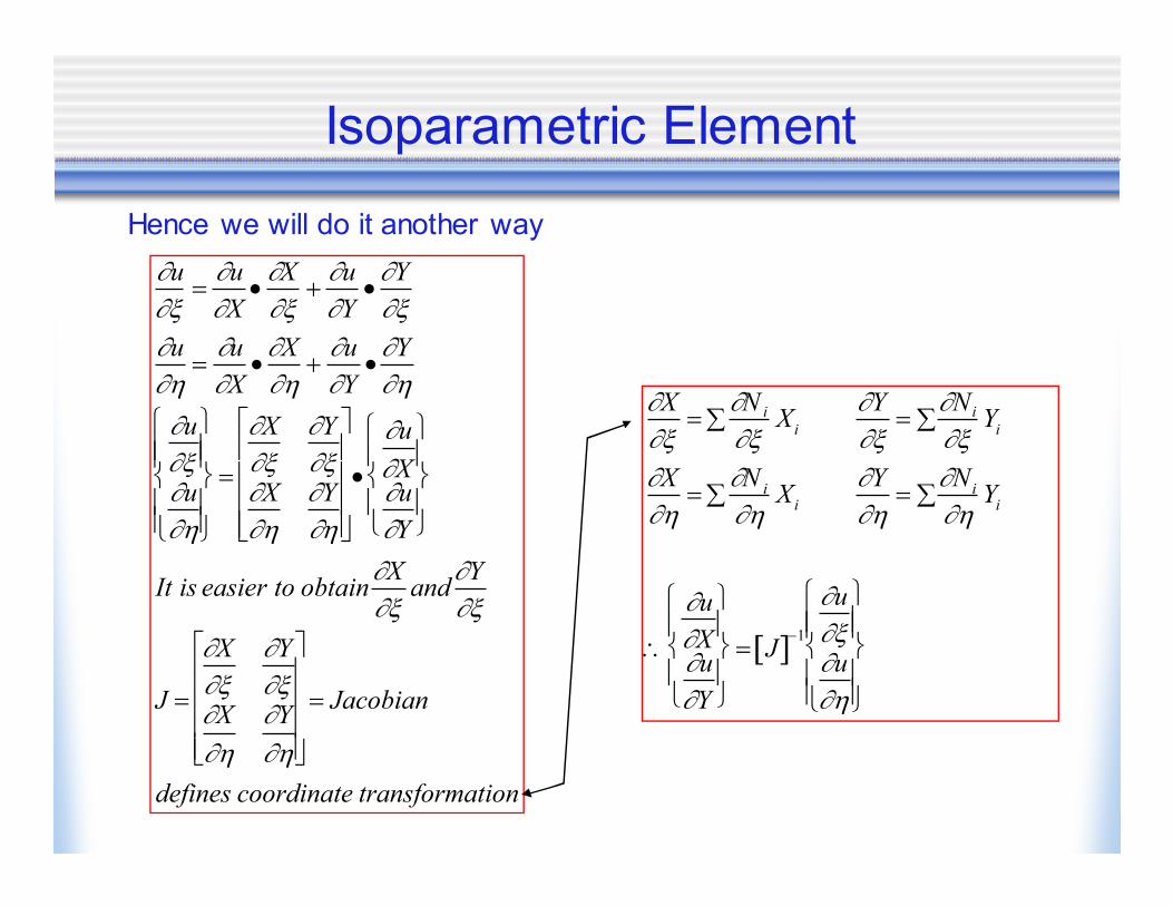
Isoparametric Element
∂u∂ξ
=∂u∂X
•∂X∂ξ
+∂u∂Y
•∂Y∂ξ
∂u∂η
=∂u∂X
•∂X∂η
+∂u∂Y
•∂Y∂η
∂u∂ξ∂u∂η
=
∂X∂ξ
∂Y∂ξ
∂X∂η
∂Y∂η
•
∂u∂X∂u∂Y
It is easier to obtain∂X∂ξ
and∂Y∂ξ
J =
∂X∂ξ
∂Y∂ξ
∂X∂η
∂Y∂η
= Jacobian
defines coordinate transformation
Hence we will do it another way
∂X∂ξ
=∂N i
∂ξX
i∑∂Y∂ξ
=∂N i
∂ξYi∑
∂X∂η
=∂N
i
∂ηX
i∑∂Y∂η
=∂N
i
∂ηYi∑
∴
∂u∂X∂u∂Y
= J[ ]−1
∂u∂ξ∂u∂η

Isoparametric Element
εx =∂u∂X
= J11
* ∂u∂ξ
+ J12
* ∂u∂η
where J11
* and J12
* are coefficients in the first row of
J[ ]−1
and∂u∂ξ
=∂N i
∂ξui and∑
∂u∂η
=∂N i
∂ηui∑
The remaining strains
εy and εxy are computed similarly
The element stiffness matrix
dX dY=|J| dξdη
k[ ] = B[ ]T E[ ]∫ B[ ]dV = B[ ]T E[ ]−1
1
∫−1
1
∫ B[ ] t J dξ dη

Gauss Quadrature
• The mapping approach requires us to be able to evaluate
the integrations within the domain (-1?1) of the functions
shown.
• Integration can be done analytically by using closed-form formulas from a table of integrals (Nah..)
� Or numerical integration can be performed
• Gauss quadrature is the more common form of numerical integration - better suited for numerical analysis and finite
element method.
• It evaluated the integral of a function as a sum of a finite
number of terms
I = φ dξ becomes I ≈ Wiφii=1
n
∑−1
1
∫

Gauss Quadrature
• Wi is the ‘weight’ and φi is the value of f(ξ=i)

Gauss Quadrature
• If φ=φ(ξ) is a polynomial function, then n-point Gauss quadrature yields the exact integral if φ is of degree 2n-1 or less.
� The form φ=c1+c2ξ is integrated exactly by the one point rule
� The form φ=c1+c2ξ+c2ξ2 is integrated exactly by the two point rule
� And so on?
� Use of an excessive number of points (more than that required) still yields the exact result
• If φ is not a polynomial, Gauss quadrature yields an approximate result.
� Accuracy improves as more Gauss points are used.
� Convergence toward the exact result may not be monotonic

Gauss Quadrature
• In two dimensions, integration is over a quadrilateral and a
Gauss rule of order n uses n2 points
• Where, WiWj is the product of one-dimensional weights.
Usually m=n.
� If m = n = 1, φ is evaluated at ξ and η=0 and I=4φ1
� For Gauss rule of order 2 - need 22=4 points
� For Gauss rule of order 3 - need 32=9 points

Gauss Quadrature
I ≈ φ1
+ φ2
+ φ3
+ φ4
for rule of order = 2
I ≈25
81(φ1+ φ
3+ φ
7+ φ
9) +40
81(φ
2+ φ
4+ φ
6+ φ
8)+64
81φ5

Number of Integration Points
• All the isoparametric solid elements are integrated numerically. Two schemes are offered: “full” integration and “reduced” integration.
� For the second-order elements Gauss integration is always used because it is efficient and it is especially suited to the polynomial product interpolations used in these elements.
� For the first-order elements the single-point reduced-integration scheme is based on the “uniform strain formulation”: the strains are not obtained at the first-order Gauss point but are obtained as the (analytically calculated) average strain over the element volume.
� The uniform strain method, first published by Flanagan and Belytschko (1981), ensures that the first-order reduced-integration elements pass the patch test and attain the accuracy when elements are skewed.
� Alternatively, the “centroidal strain formulation,” which uses 1-point Gauss integration to obtain the strains at the element center, is also available for the 8-node brick elements in ABAQUS/Explicit for improved computational efficiency.

Number of Integration Points
• The differences between the uniform strain formulation and the
centroidal strain formulation can be shown as follows:

Number of Integration Points
Number of integration points
• Numerical integration is simpler than analytical, but it is not
exact. [k] is only approximately integrated regardless of the
number of integration points
� Should we use fewer integration points for quick computation
� Or more integration points to improve the accuracy of
calculations.
� Hmm?.

Reduced Integration
• A FE model is usually inexact, and usually it errs by being too stiff.
Overstiffness is usually made worse by using more Gauss points to
integrate element stiffness matrices because additional points capture
more higher order terms in [k]
• These terms resist some deformation modes that lower order tems do
not and therefore act to stiffen an element.
• On the other hand, use of too few Gauss points produces an even worse
situation known as: instability, spurious singular mode, mechanics, zero-
energy, or hourglass mode.
� Instability occurs if one of more deformation modes happen to
display zero strain at all Gauss points.
� If Gauss points sense no strain under a certain deformation mode,
the resulting [k] will have no resistance to that deformation mode.

Reduced Integration
• Reduced integration usually means that an integration scheme one
order less than the full scheme is used to integrate the element's internal
forces and stiffness.
� Superficially this appears to be a poor approximation, but it has
proved to offer significant advantages.
� For second-order elements in which the isoparametric coordinate
lines remain orthogonal in the physical space, the reduced-
integration points have the Barlow point property (Barlow, 1976): the
strains are calculated from the interpolation functions with higher
accuracy at these points than anywhere else in the element.
� For first-order elements the uniform strain method yields the exact
average strain over the element volume. Not only is this important
with respect to the values available for output, it is also significant
when the constitutive model is nonlinear, since the strains passed
into the constitutive routines are a better representation of the actual
strains.
Reduced Integration
• Reduced integration decreases the number of constraints introduced by
an element when there are internal constraints in the continuum theory
being modeled, such as incompressibility, or the Kirchhoff transverse
shear constraints if solid elements are used to analyze bending
problems.
• In such applications fully integrated elements will “lock”—they will exhibit
response that is orders of magnitude too stiff, so the results they provide
are quite unusable. The reduced-integration version of the same
element will often work well in such cases.
• Reduced integration lowers the cost of forming an element. The
deficiency of reduced integration is that the element stiffness matrix will
be rank deficient.
• This most commonly exhibits itself in the appearance of singular modes
(“hourglass modes”) in the response. These are nonphysical response
modes that can grow in an unbounded way unless they are controlled.

Reduced Integration
• The reduced-integration second-order serendipity interpolation elements
in two dimensions—the 8-node quadrilaterals—have one such mode, but
it is benign because it cannot propagate in a mesh with more than one
element.
• The second-order three-dimensional elements with reduced integration
have modes that can propagate in a single stack of elements. Because
these modes rarely cause trouble in the second-order elements, no
special techniques are used in ABAQUS to control them.
• In contrast, when reduced integration is used in the first-order elements
(the 4-node quadrilateral and the 8-node brick), hourglassing can often
make the elements unusable unless it is controlled.
• In ABAQUS the artificial stiffness method given in Flanagan and
Belytschko (1981) is used to control the hourglass modes in these
elements.

Reduced Integration
The FE model will have no resistance to loads that activate these modes.
The stiffness matrix will be singular.

Reduced Integration
• Hourglass mode for 8-node element with reduced
integration to four points
• This mode is typically non-communicable and will not occur
in a set of elements.

Reduced Integration
• The hourglass control methods of Flanagan and Belytschko (1981) are
generally successful for linear and mildly nonlinear problems but may
break down in strongly nonlinear problems and, therefore, may not yield
reasonable results.
• Success in controlling hourglassing also depends on the loads applied
to the structure. For example, a point load is much more likely to trigger
hourglassing than a distributed load.
• Hourglassing can be particularly troublesome in eigenvalue extraction
problems: the low stiffness of the hourglass modes may create many
unrealistic modes with low eigenfrequencies.
• Experience suggests that the reduced-integration, second-order
isoparametric elements are the most cost-effective elements in
ABAQUS for problems in which the solution can be expected to be
smooth.

Solving Linear Equations
• Time independent FE analysis requires that the global
equations [K]{D}={R} be solved for {D}
• This can be done by direct or iterative methods
• The direct method is usually some form of Gauss
elimination.
• The number of operations required is dictated by the number of d.o.f. and the topology of [K]
• An iterative method requires an uncertain number of
operations; calculations are halted when convergence
criteria are satisfied or an iteration limit is reached.

Solving Linear Equations
• If a Gauss elimination is driven by node numbering, forward
reduction proceeds in node number order and back
substitution in reverse order, so that numerical values of
d.o.f at first numbered node are determined last.
• If Gauss elimination is driven by element numbering,
assembly of element matrices may alternate with steps of
forward reduction.
� Some eliminations are carried out as soon as enough
information has been assembled, then more assembly is
carried out, then more eliminations, and so on?
� The assembly-reduction process is like a ‘wave’ that moves
over the structure.
� A solver that works this way is called a wavefront or ‘frontal’
equation solver.

Solving Linear Equations
• The computation time of a direct solution is roughly
proportional to nb2, where n is the order of [K] and b is the
bandwidth.
� For 3D structures, the computation time becomes large
because b becomes large.
� Large b indicates higher connectivity between the degrees of
freedom.
� For such a case, an iterative solver may be better because
connectivity speeds convergence.

Solving Linear Equations
• In most cases, the structure must be analyzed to determine
the effects of several different load vectors {R}.
� This is done more effectively by direct solvers because most
of the effort is expended to reduce the [K] matrix.
� As long as the structure [K] does not change, the
displacements for the new load vectors can be estimated
easily.
� This will be more difficult for iterative solvers, because the
complete set of equations need to be re-solved for the new
load vector.
� Iterative solvers may be best for parallel processing computers
and nonlinear problems where the [K] matrix changes from
step i to i+1. Particularly because the solution at step i will be
a good initial estimate.

Symmetry conditions
• Types of symmetry include reflective, skew, axial and cyclic.
If symmetry can be recognized and used, then the models
can be made smaller.
� The problem is that not only the structure, but the boundary
conditions and the loading needs to be symmetric too.
� The problem can be anti-symmetric
� If the problem is symmetric
� Translations have no component normal to a plane of
symmetry
� Rotation vectors have no component parallel to a plane of
symmetry.

Symmetry conditions
Plane of Symmetry
(Restrained
Motions)
Plane of Anti-symmetry
(Restrained
Motions)

Symmetry Conditions

Constraints
• Special conditions for the finite element model.
� A constraint equation has the general form [C]{D}-{Q}=0
� Where [C] is an mxn matrix; m is the number of constraint equation, and n is the number of d.o.f. in the global vector {D}
� {Q} is a vector of constants and it is usually zero.
� There are two ways to impose the constraint equations on the global equation [K]{D}={R}
• Lagrange Multiplier Method
� Introduce additional variables known as Lagrange multipliers λ={λ1 λ2
λ3 ? λm}T
� Each constraint equation is written in homogenous form and multiplied by the corresponding λI which yields the equation λ
� λΤ{[C]{D} - {Q}}=0
� Final FormK CT
C 0
D
λ
=R
Q
Solved by Gaussian E limination
Constraints
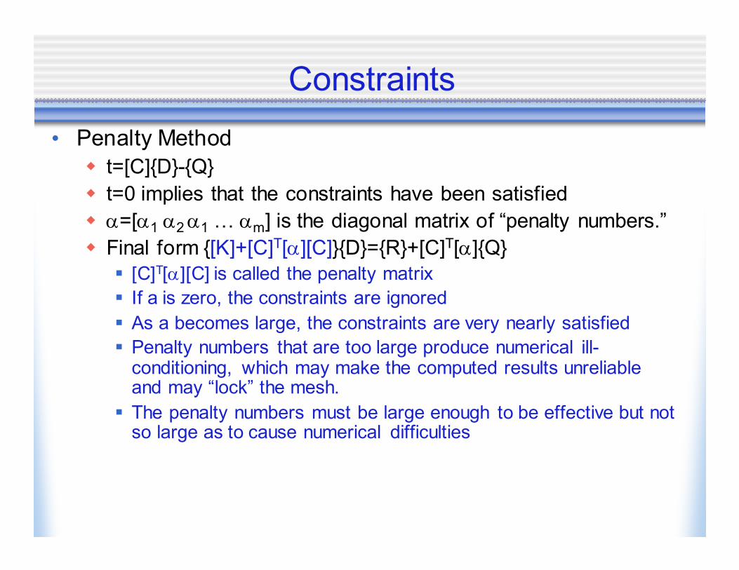
• Penalty Method
� t=[C]{D}-{Q}
� t=0 implies that the constraints have been satisfied
� α=[α1 α2 α1 ? αm] is the diagonal matrix of “penalty numbers.”
� Final form {[K]+[C]T[α][C]}{D}={R}+[C]T[α]{Q}
� [C]T[α][C] is called the penalty matrix
� If a is zero, the constraints are ignored
� As a becomes large, the constraints are very nearly satisfied
� Penalty numbers that are too large produce numerical ill-conditioning, which may make the computed results unreliable and may “lock” the mesh.
� The penalty numbers must be large enough to be effective but not so large as to cause numerical difficulties
3D Solids and Solids of Revolution
• 3D solid - three-dimensional solid that is unrestricted as to
the shape, loading, material properties, and boundary
conditions.
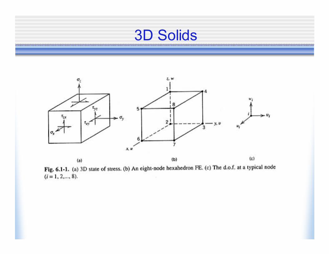
• All six possible stresses (three normal and three shear) must be taken into account.
� The displacement field involves all three components (u, v,
and w)
� Typical finite elements for 3D solids are tetrahedra and
hexahedra, with three translational d.o.f. per node.
3D Solids

3D Solids
• Problems of beam bending, plane stress, plates and so on
can all be regarded as special cases of 3D solids.
� Does this mean we can model everything using 3D finite
element models?
� Can we just generalize everything as 3D and model using 3D
finite elements.
• Not true! 3D models are very demanding in terms of
computational time, and difficult to converge.
� They can be very stiff for several cases.
� More importantly, the 3D finite elements do not have rotational
degrees of freedom, which are very important for situations
like plates, shells, beams etc.

3D Solids
• Strain-displacement relationships

3D Solids
• Stress-strain-temperature relations

3D Solids
• The process for assembling the element stiffness matrix is
the same as before.
� {u}=[N] {d}
� Where, [N] is the matrix of shape functions
� The nodes have three translational degrees of freedom.
� If n is the number of nodes, then [N] has 3n columns

3D Solids
• Substitution of {u}=[N]{d} into the strain-displacement
relation yields the strain-displacement matrix [B]
• The element stiffness matrix takes the form:

3D Solid Elements
• Solid elements are direct extensions of plane elements
discussed earlier. The extensions consist of adding another
coordinate and displacement component.
� The behavior and limitations of specific 3D elements largely
parallel those of their 2D counterparts.
• For example:
� Constant strain tetrahedron
� Linear strain tetrahedron
� Trilinear hexahedron
� Quadratic hexahedron
• Hmm?
� Can you follow the names and relate them back to the planar
elements

3D Solids
• Pictures of solid elements
CSTLST Q4
Q8

3D Solids
• Constant Strain Tetrahedron. The element has three
translational d.o.f. at each of its four nodes.
� A total of 12 d.o.f.
� In terms of generalized coordinates βi its displacement field is
given by.
� Like the constant strain triangle, the constant strain
tetrahedron is accurate only when strains are almost constant
over the span of the element.
� The element is poor for bending and twisting specially if the
axis passes through the element of close to it.
3D Solids
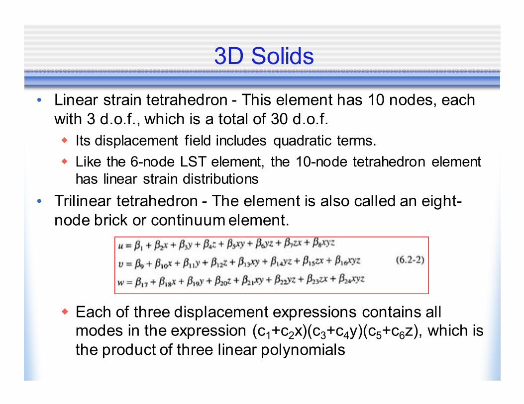
• Linear strain tetrahedron - This element has 10 nodes, each
with 3 d.o.f., which is a total of 30 d.o.f.
� Its displacement field includes quadratic terms.
� Like the 6-node LST element, the 10-node tetrahedron element
has linear strain distributions
• Trilinear tetrahedron - The element is also called an eight-
node brick or continuum element.
� Each of three displacement expressions contains all modes in the expression (c1+c2x)(c3+c4y)(c5+c6z), which is
the product of three linear polynomials

3D Solids
• The hexahedral element can be of arbitrary shape if it is
formulated as an isoparametric element.

3D Solids
• The determinant |J| can be regarded as a scale factor. Here
it expresses the volume ratio of the differential element dX
dY dZ to the dξ dη dζ• The integration is performed numerically, usually by 2 x 2 x
2 Gauss quadrature rule.
• Like the bilinear quadrilateral (Q4) element, the trilinear
tetrahedron does not model beam action well because the sides remain straight as the element deforms.
• If elongated it suffers from shear locking when bent.
• Remedy from locking - use incompatible modes - additional degress of freedom for the sides that allow them to curve

3D Solids
• Quadratic Hexahedron
� Direct extension of the quadratic quadrilateral Q8 element
presented earlier.
� [B] is now a 6 x 60 rectangular matrix.
� If [k] is integrated by a 2 x 2 Gauss Quadrature rule, three
“hourglass” instabilities will be possible.
� These hourglass instabilities can be communicated in 3D
element models.
� Stabilization techniques are used in commercial FE packages.
Their discussion is beyond the scope.

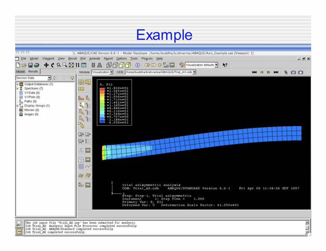
Example - Axisymmetric elements
d
123in.
9 in.
1 ksi

Example

Example

Example

Example

Example

Example

Example

Example

Example
Example

Example


