Finite-element simulation of buoyancy-driven turbulent ows · Finite-element simulation of...

Finite-element simulationof

buoyancy-driven turbulent flows

Dissertation

zur Erlangung des Doktorgradesder Mathematisch-Naturwissenschaftlichen Fakultaten

der Georg-August-Universitat zu Gottingen

vorgelegt von

Tobias Knopp

aus

Lubeck

Gottingen 2003

D7

Referent: Prof. Dr. G. Lube

Korreferent: Prof. Dr. R. Schaback

Tag der mundlichen Prufung: 4. Juni 2003

2

Contents

Preface 7

Epitome . . . . . . . . . . . . . . . . . . . . . . . . . . . . . . . . . . . . . . . . . 8Acknowledgements . . . . . . . . . . . . . . . . . . . . . . . . . . . . . . . . . . . 9

I. Turbulence modelling for buoyancy driven flows 11

1. The laminar model 13

1.1. Laminar thermally coupled flow problems . . . . . . . . . . . . . . . . . . . 131.2. Boundary conditions for thermally coupled flows . . . . . . . . . . . . . . . 151.3. A model for non-isothermal flow problems . . . . . . . . . . . . . . . . . . . 181.4. Modelling turbulent boundary layers using a fully overlapping DDM . . . . 19

2. Fundamentals, modelling and simulation of turbulent flows 23

2.1. Aspects of randomness and statistical description of turbulent flows . . . . 232.2. The scales of turbulent flows . . . . . . . . . . . . . . . . . . . . . . . . . . 262.3. Criteria for appraising approaches in CFD . . . . . . . . . . . . . . . . . . . 27

3. The k/ε turbulence model 29

3.1. The Reynolds averaged Navier-Stokes equations . . . . . . . . . . . . . . . . 293.2. Turbulent-viscosity and gradient-diffusion hypotheses . . . . . . . . . . . . . 303.3. Production and dissipation of turbulent kinetic energy in RANS models . . 333.4. A two-equation model : The k/ε model . . . . . . . . . . . . . . . . . . . . 34

4. Large-eddy simulation 39

4.1. Filtering . . . . . . . . . . . . . . . . . . . . . . . . . . . . . . . . . . . . . . 394.2. Differential filtering . . . . . . . . . . . . . . . . . . . . . . . . . . . . . . . . 414.3. The space averaged non-isothermal Navier-Stokes equations . . . . . . . . . 424.4. Modelling the residual stress tensor and the residual fluxes . . . . . . . . . . 444.5. System of equations for non-isothermal LES . . . . . . . . . . . . . . . . . . 49

5. Near-wall treatment in turbulence modelling 51

5.1. Fundamentals of turbulent boundary-layer theory . . . . . . . . . . . . . . . 515.2. Boundary-layer equations and singular perturbation methods . . . . . . . . 535.3. Algebraic turbulence models for non-isothermal boundary layers . . . . . . 595.4. Algebraic turbulence models for natural convection boundary layers . . . . 635.5. On the near-wall behaviour of the k/ε model . . . . . . . . . . . . . . . . . 655.6. On LES in the near-wall region . . . . . . . . . . . . . . . . . . . . . . . . . 66

3

6. A computational k/ε model using wall functions 676.1. A two-domain approach . . . . . . . . . . . . . . . . . . . . . . . . . . . . . 676.2. The wall function concept as a fully overlapping DDM . . . . . . . . . . . . 686.3. The wall function concept using boundary-layer theory . . . . . . . . . . . . 70

7. A computational LES model 757.1. Wall stress models . . . . . . . . . . . . . . . . . . . . . . . . . . . . . . . . 777.2. Hybrid RANS/LES approaches . . . . . . . . . . . . . . . . . . . . . . . . . 80

8. Some analytical results for LES with near wall modelling 818.1. Some simplifications of the coupled problem . . . . . . . . . . . . . . . . . . 828.2. A separate study of global and local subproblem . . . . . . . . . . . . . . . 848.3. The coupled steady state problem . . . . . . . . . . . . . . . . . . . . . . . 948.4. Some closing remarks . . . . . . . . . . . . . . . . . . . . . . . . . . . . . . 106

II. Numerical solution scheme and numerical tests 111

9. Semidiscretisation in time, decoupling and linearisation 1139.1. Semidiscretisation in time using the discontinuous Galerkin method . . . . 1139.2. Semidiscretisation, decoupling, and linearisation for the k/ε model . . . . . 1149.3. Semidiscretisation, decoupling, and linearisation for the LES model . . . . . 1179.4. Variational formulation of the arising model problems . . . . . . . . . . . . 120

10.Discretisation in space using stabilised FEM 12110.1. Finite-element discretisation for ADR-problems . . . . . . . . . . . . . . . . 12110.2. Stabilisation techniques for ADR-problems . . . . . . . . . . . . . . . . . . . 12110.3. Discontinuity capturing for ADR-problems . . . . . . . . . . . . . . . . . . . 12310.4. Finite-element discretisation for Oseen problems . . . . . . . . . . . . . . . 12410.5. SUPG- und PSPG-stabilisation for Oseen problems . . . . . . . . . . . . . . 124

11.Non-overlapping domain decomposition methods 12711.1. The Robin-Robin algorithm for advection-diffusion-reaction problems . . . . 12811.2. Choice of the interface function in the R-R-algorithm for ADR problems . . 12911.3. The Robin-Robin algorithm for Oseen type problems . . . . . . . . . . . . . 130

12.Turbulent channel flow 13312.1. Fundamentals of isothermal channel flow . . . . . . . . . . . . . . . . . . . . 13312.2. Isothermal channel flow computations using the k/ε model . . . . . . . . . . 13612.3. Quasi a priori testing of the SGS model . . . . . . . . . . . . . . . . . . . . 138

13.Turbulent natural convection in an air filled square cavity 15113.1. Introduction . . . . . . . . . . . . . . . . . . . . . . . . . . . . . . . . . . . . 15113.2. Description of the flow configuration . . . . . . . . . . . . . . . . . . . . . . 15213.3. Testing the wall iteration concept . . . . . . . . . . . . . . . . . . . . . . . . 15413.4. A posteriori testing for the k/ε model without DDM . . . . . . . . . . . . . 157

13.5. A posteriori testing for the k/ε model with DDM . . . . . . . . . . . . . . . 16013.6. Appraisal of the k/ε model predictions . . . . . . . . . . . . . . . . . . . . 16613.7. First results for the posteriori testing using LES . . . . . . . . . . . . . . . 167

14.Summary and future prospects 175

III. Appendix 177

A. Mathematical tools for residual stress modelling in LES 179A.1. Fourier transformation, convolution and distributions . . . . . . . . . . . . . 179A.2. Closure approximations for LES . . . . . . . . . . . . . . . . . . . . . . . . . 183

B. Some mathematical tools for the Navier-Stokes equations 187B.1. Functional analytic fundamentals . . . . . . . . . . . . . . . . . . . . . . . . 187B.2. Analytical results for some turbulence models . . . . . . . . . . . . . . . . . 191

C. Turbulent boundary-layer theory 193C.1. Natural convection turbulent boundary layers . . . . . . . . . . . . . . . . . 193C.2. Forced convection boundary-layer equations in non-dimensional form . . . . 195C.3. The universal log law by Prandtl and van Karman . . . . . . . . . . . . . . 196C.4. A non-isothermal wall law for forced convection problems by Neitzke . . . . 197

D. Nomenclature 199

Bibliography 206

Curriculum vitae 219

5

6

Preface

Turbulent flows driven or significantly affected by buoyancy occur in a variety of problemsincluding building ventilation, cooling of electrical equipment, and environmental science.The fundamental mathematical model are the non-isothermal Navier-Stokes equations, gov-erning the time-evolution of velocity u, pressure p, and temperature T . The phenomenonof turbulence reveals that their solutions can become very complex if a critical parameter,e.g., the Reynolds number or the Rayleigh number, becomes large. A proper numericalresolution of the random motion of all scales of u, p, and T (called Direct Numerical Simu-lation) is feasible only for a very limited number of flows. Thus the major task in turbulencemodelling is to reduce the complexity of the Navier-Stokes equations in a manner which isappropriate to the needs of science and engineering. The goal is to develop models that arecomputationally simpler than the Navier-Stokes equations but ”whose predictions are closeto those of the Navier-Stokes equations”. In this thesis we pursue two strategies: The firstapproach is a statistical approach which is based on a statistical averaging procedure forthe Navier-Stokes equations. The objective is to obtain a set of equations for the statisticalmean values for u, p, and T , which requires an empirical modelling of the terms involvingstatistical fluctuations. The second approach is called large-eddy simulation (LES). Theidea of LES is to apply a spatial averaging filter to the Navier-Stokes equations in order toextract the large-scale structures of u, p, and T , and to attenuate their small-scale struc-tures. Then only the random motion of the large scales is resolved and the effects of thesmall scales on the large scales are modelled.This thesis is involved into a longlasting cooperation with the Institute for Thermodynam-ics and Building Energy Systems at Dresden University of Technology. A major resultof this cooperation is our research code ParallelNS, see e.g. [Mue99] and [KLGR02].ParallelNS is intended for the numerical solution of indoor-air flow problems, see e.g.[Gri01]. The building blocks of this code are the k/ε model (which is a statistical turbulencemodel), an improved wall-function concept for the treatment of the near-wall region, anda stabilised finite-element method together with an iterative substructuring method as adomain decomposition method for the numerical solution process.The first objective of this thesis is a critical review of the theoretical background of thesebuilding blocks. Both the turbulence model and the numerical solution scheme used in Par-

allelNS are described in a manner which is more convenient to mathematicians than thepresentations in engineering textbooks. Secondly, the aim is to investigate the accuracy ofour research code. The near-wall treatment in ParallelNS conceived by [Nei99] had notyet been assessed by reference with experimental data from other research groups. We willinvestigate a natural convection flow in an air filled cavity. For this test case Karayiannis

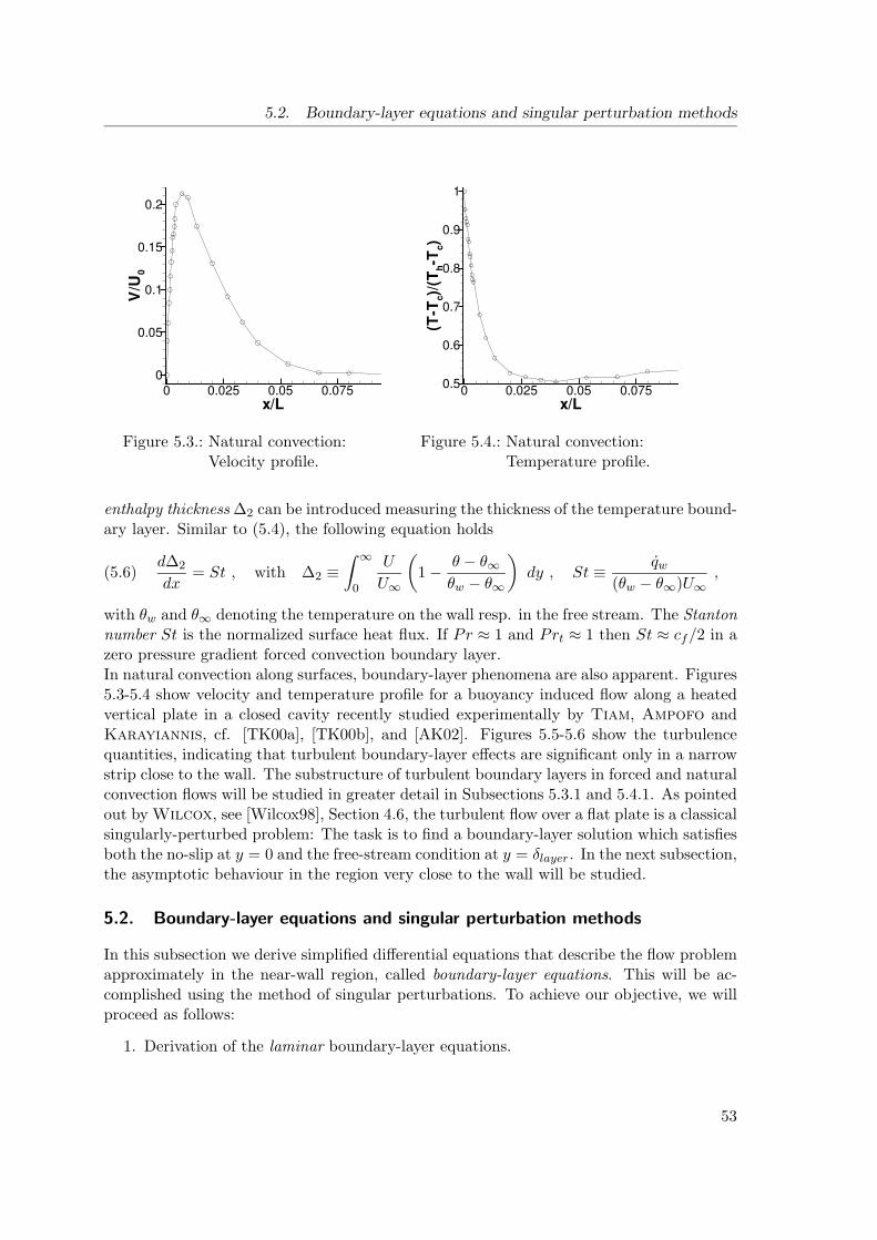
et al. (see [TK00a] and [AK02]) provided widely accepted experimental data. Moreoverthe accuracy of the domain decomposition method for this three-dimensional test case hasto be investigated, since the numerical tests in [Mue99] are restricted to two-dimensionalproblems.

7

The k/ε model is the most widespread turbulence model, but it suffers from severalwell-known deficiencies. Thus an additional objective of this thesis is to recommend al-ternative turbulence models which are amenable for use in ParallelNS. A successfulimprovement of the standard k/ε model is the so called k-ε-v2 model, which was de-vised by Durbin, see [Dur91]. However, this model requires resolving the near-wall re-gion, which is infeasible for three-dimensional problems of practical relevance. Thereforewe study LES, which has the additional advantage of being much closer to the Navier-Stokes equations than statistical turbulence models. Modern advances in computer powerhave allowed LES to become more and more interesting for engineering applications, see,e.g., the current projects in Prof. Dr. Lars Davidson’s research group at the Depart-ment of Thermo and Fluid Dynamics at Chalmers University of Technology Goteborg(http://www.tfd.chalmers.se/∼lada/projects/proind.html) and the homepage of the FlowPhysics and Computation Division at the Department of Mechanical Engineering at Stan-ford University (http://www-fpc.stanford.edu/). The objective of this thesis is not to devisenew LES models but to review current models in order to employ them in ParallelNS.LES models are often referred to as residual stress models. Three residual stress modelshave been studied in this thesis, viz., the well-known Smagorinsky model, the Iliescu-Laytonmodel (see [IL98]), and the Galdi-Layton model (see [GL00]), including a modification de-vised by Eidson, cf. [Eid85]. We describe how these models can be applied in a naturalmanner in ParallelNS using the same near-wall strategy as for the k/ε model. We per-form an a priori test and show first results from an a posteriori test. An a priori test usesexperimental data or data from a DNS to study the residual stress model separately. In an aposteriori test, we perform a computation for a certain flow problem and then compare thecalculated statistics (mean values, variances) with the corresponding statistics extractedfrom experimental data or from a DNS.The wall function concept applied in ParallelNS can be viewed as a fully overlappingdomain decomposition method, as devised by Tidriri and LeTallec, cf. [LTT99]. Withinthis approach, a boundary-layer solution is determined in the near-wall region, which sat-isfies the correct Dirichlet boundary condition at the wall and which is matched with theglobal solution on an artificial inner boundary. The crucial point is that the boundary-layer information is transferred to the global problem using a suitable friction (Neumann)boundary condition for the global problem. From a mathematical point of view this ap-proach is not yet well understood. During a research stay at the University of Pittsburgh,in close cooperation with Prof. Dr. W. J. Layton some mathematical results for a certaincoupling scheme have been obtained, which will be presented in this thesis.

Epitome

Part I is dedicated to a detailed description of the turbulence models studied in this thesis.In Chapter 1 the laminar case is studied and the wall function procedure is motivated.In Chapter 2 some fundamental results regarding turbulent flows and their modelling arereviewed. Chapter 3 is devoted to the k/ε turbulence model and in Chapter 4 some LESmodels are described. In Chapter 5 we derive a set of appropriate boundary-layer equationsfor the near-wall region. In Chapters 6 we present the k/ε model using the wall-functionprocedure which is implemented in our research code. The corresponding computational

8

model for the LES models is described in Chapter 7. Chapter 8 is dedicated to the analysisof a certain wall-function scheme for LES.Part II is devoted to a description of the numerical solution scheme and to the numericalinvestigations. In Chapter 9 we study the semidiscretisation in time and the linearisationfor both models. The spatial discretisation is considered in Chapter 10. The domaindecomposition method will be described in Chapter 11. Numerical tests for the fullydeveloped turbulent channel flow and for a natural convection flow in a closed cavity arestudied in Chapters 12 and 13 resp.In the appendix, some prerequisited material is reviewed. Moreover, some additional resultswill be presented there, which do not fit well into the thread of principal ideas in the maintext.

Acknowledgements

I am profoundly grateful to many people for their kind assistance and support in writingthis thesis. First, I would like to thank my adviser Prof. Dr. G. Lube for providing methe opportunity to pursue a PhD in his research group und for his continual support. Thisthesis has benefited immeasurably from his revisions and advices. Moreover I am verygrateful to Gerd Rapin for many valuable discussions on numerical analysis and on domaindecomposition methods. My sincere thanks are given to Andreas Priesnitz for his kindassistance in administrating the software used for this thesis. I am very grateful to MarkusRosler, Hannes Muller, Ralf Gritzki, and Joachim Seifert (Institute for Thermodynamicsand Building Energy Systems at TU Dresden) for their kind assistance regarding our re-search code ParallelNS throughout the last years. For his valuable suggestions, for hisencouraging stimulus and for his kind support during my research stay in Pittsburgh, Iwould like to give my genuine thanks to Prof. Dr. W. J. Layton (Department of Mathe-matics at Pittsburgh University). I would also like to thank him and his family for theirkind hospitality during my first days in Pittsburgh. I gratefully acknowledge the hospi-tality of the University of Pittsburgh and I would like to thank Tony DiGiorno and DrewPorvaznik for their strong help. Similarly, I am very grateful to Adrian Dunca, TraianIliescu, Dr. habil. Volker John, Dr. Holger Frahnert, Dr. Claus Wagner, Felix Ampofo,and Dr. Shia-Hui Peng for valuable discussions and communications. I would also liketo express appreciation to our system administrators Dr. Gerhard Siebrasse, Rolf Wass-mann, Joachim Perske, and Klaus Konnecke for their excellent support. Moreover I amvery grateful to the Institute for Numerical and Applied Mathematics at Gottingen Uni-versity for providing me an excellent working environment. I would like to give my sincerethanks to Mrs. Kalz and to my mother for reading over parts of this thesis for correct useof the English language. I would like to apologise to those, who suffered obstructions inavailable computing resources due to my own numerical tests during the last few months.For the generous financial support, I am very grateful to my sponsor ”Graduiertenkollegfur Stromungsinstabilitaten und Turbulenz”.For their terrific friendship I am very grateful to my very best friends Matthias, Markus,Niklas and Florian. Finally, I would like to thank my family. They have supported mewith great patience and loving care throughout my life and taught me the right things.

9

10

Part I.

Turbulence modelling for buoyancy driven flows

11

1. The laminar model

The first part of this thesis is devoted to turbulence modelling for incompressible buoyancydriven flows. We begin by considering the laminar case, introducing the incompressiblenon-isothermal Navier-Stokes equations. These are the governing equations for velocity,pressure and temperature in non-isothermal flow problems.

1.1. Laminar thermally coupled flow problems

Let Ω be an open domain of Rd (d = 2, 3) and Γ its (sufficiently regular, at least Lipschitzcontinuous) boundary. Denote u the velocity field, p the pressure and T the temperature.Note that in the sequel dimensional variables are labelled by a tilde. Then the time evolu-tion of these quantities is described by the following coupled system of partial differentialequations:

ρ

(∂u

∂t+ (u · ∇)u

)− ∇ · ( 2 µS ( u ) ) + ∇ p = ρ g ,(1.1)

∇ · u = 0 ,(1.2)

ρ cp

(∂T

∂t+ ( u · ∇ ) T

)− ∇ ·

(λ∇ T

)= ˜qV(1.3)

together with a set of initial and boundary conditions to be discussed later in this section.µ is the dynamic viscosity of the fluid and ρ its density. g is the gravitational acceleration,cp denotes the specific heat at constant pressure, λ (often used alternative symbol: k) isthe thermal conduction coefficient, and ˜qV is a volume specific external heat source. Eq.(1.1) is called momentum equation. We use the symmetric, deviatoric rate-of-strain tensor

S ( u ) =∇u+∇uT

2, ∇su ≡ 2 S ( u ) .

Eq. (1.2) ensures the incompressibility of the fluid and is called equation of continuity.Eq. (1.3) will be referred to as temperature equation or heat transfer equation. Note thatin indoor-air flow problems it is reasonable to neglect the dissipation of mechanical work(Joule effect) and heat transfer via radiation in (1.3).In thermally coupled flow problems, the governing equations are fully coupled. First, asdensity is temperature sensitive, temperature variations may lead to density gradients. Thiscan result in buoyancy forces due to gravitational forces. These are taken into account bythe right hand side term in (1.1). For this reason temperature is referred to as an ’active’scalar in (1.1). Second, the velocity field is the convection field for the temperature in (1.3).The density dependence on the temperature is modelled by using the so-called Boussinesq

13


approximation, which consists of two parts. First, it assumes that ρ(T ) behaves like

ρ(T ) = ρ0 − ρ0β0(T − T0) , with ρ0 ≡ ρ(T0) , β0 ≡ − 1ρ

(∂ρ

∂T

)∣∣∣∣T=T0

(1.4)

and β0 being the volumetric coefficient of thermal expansion. T0 is a reference temperature.This equation can be regarded as a Taylor expansion of ρ around T0 (while keeping thepressure constant). Second, it assumes that density variations can be neglected in inertialterms, but not when they are multiplied by gravity, see e.g. [DPR01], p.223.

Remark 1.1References concerning the thermodynamical background of the Boussinesq approximationcan be found e.g. in [Cod93b], p.3.2. According to [Mue91] the Boussinesq approximationis accurate enough for temperature differences of about 50 K. This is satisfied in typicalindoor-air flow problems. ♦

Now we introduce a reduced pressure

pred ≡ p− ρ0g · x .(1.5)

Using the Boussinesq approximation and the reduced pressure, (1.1)-(1.3) can be rearrangedto

ρ0

(∂u

∂t+ (u · ∇)u

)− ∇ · ( 2 µS ( u ) ) + ∇ pred = − ρ0 β0 ( T − T0 ) g ,(1.6)

∇ · u = 0 ,(1.7)

ρ0 cp

(∂T

∂t+ ( u · ∇ ) T

)− ∇ ·

(λ∇ T

)= ˜qV .(1.8)

It is convenient to write the (non-isothermal) Navier-Stokes equations in a non-dimensionalform, i.e. with respect to the following scaled variables:

t ≡ tUsc

L, x ≡ x

L, u ≡ u

Usc, θ ≡ T − T0

Tdiff.

Here, L is a characteristic length of the problem, Tdiff is a characteristic temperaturedifference, and Usc is a suitable velocity scale (which will be determined later in this section).Recall that in fluid mechanics the following dimensionless numbers are defined, see e.g.[KC93]:

Re ≡ ρ0LUscµ

, Reynolds number, P r ≡ cpµ

λ, Prandtl number,

Gr ≡β0|g|ρ2

0L3Tdiff

µ2, Grashof number, Ra ≡

β0|g|cpρ20L

3Tdiff

µλ, Rayleigh number.

We introduce the thermal diffusivity a ≡ λ/(cpρ0) and the kinematic viscosity ν ≡ µ/ρ0.Note that Pr = νa−1. The numbers are related by Ra = GrPr. From these relations it

14

1.2. Boundary conditions for thermally coupled flows

can be seen that the Prandtl number is a measure for the similarity of the transport ofheat and momentum. The Grashof number is the ratio of the buoyancy force to the viscousforce.Depending on the boundary conditions for the momentum equation, there are two differentpossibilities for choosing a characteristic scaling velocity Usc. In the case of so-called forcedconvection, the fluid motion is enforced by the boundary conditions (see section 1.2). Thenwe choose Usc = ||u||∞,Γ. In indoor-air flow problems most of the time there is no externalforce and u = 0 or a homogeneous Neumann condition is prescribed on the boundary.The only driving forces are due to buoyancy effects. Then physically meaningful choiceis Usc = (β0|g|Tdiff L)1/2, cf. [KC93], p.408. In both cases the reduced pressure is non-dimensionalised with ρ0U

2sc.

Remark 1.2As it will turn out in Section 10.5, an appropriate choice for Usc is essential for the PSPG-stabilisation technique in the numerical solution process. ♦

In this thesis dimensionless quantities are chosen in agreement with [Mue99], viz.,

a ≡ λ

cpρ0, a ≡ a

LUsc, g ≡ gL

U2sc

, cp ≡λTdiff

ρ0aU2sc

, qV ≡˜qV Lρ0U3

sc

, β ≡ β0Tdiff , ν ≡µ

ρ0UscL.

This yields the following system of equations

∂tu−∇ · ( 2 ν S(u) ) + (u ·∇)u+∇pred = − β θ g ,(1.9)∇ · u = 0 ,(1.10)

∂tθ + (u ·∇)θ −∇ · (a∇θ) = qV c−1p .(1.11)


For specifying the boundary conditions, we introduce two partitions of Γ : one for themomentum equation and one for all scalar equations, e.g., the heat transfer equation anda possible additional equation describing contaminant transport.

The first partition of Γ is due to the boundary conditions concerning the momentum equa-tion. For this purpose we define the stress tensor

σ(u, p) = − pI + 2νS(u) .

Moreover we suppose that for almost every point x in Γ we have a local orthonormal basisn(x) , tj(x) , 1 ≤ j ≤ d− 1, where tjd−1

j=1 is a local orthonormal basis for the tangentspace of Γ in x and n denotes the outer unit normal vector to Γ at x. Denote

ΓF = x ∈ Γ | u = uF , uF · n < 0 a.e. in ΓF ,(1.12)

ΓW = x ∈ Γ | u · n = 0 , χnTσ(u, p)tj = σt(u) · tj 1 ≤ j ≤ d− 1 ,(1.13)ΓN = x ∈ Γ | σ(u, p)n = σn (1.14)

15


which are mutually disjoint and satisfy ΓF ∪ ΓN ∪ ΓW = Γ. The quantity nTTr|ΓW σ(u, p)is called stress vector, which represents the force that the fluid exerts on the wall. HereTr|ΓW denotes the trace operator, see Chapter B and Remark 8.4. ΓF is a forced convectioninflow boundary; on ΓF a non-zero inflow velocity profile is prescribed. (1.13) describes ageneral (non-linear) friction law, covering the following situations:

(i) slip with linear friction: χ ≡ 1, and σt(u) · tj ≡ −βju · tj ,

(ii) wall stress condition: χ ≡ 1, and σt(u) · tj ≡ τw u·tj||u·tj ||

(provided u · tj 6= 0),

(iii) no-slip condition: χ = 0, and σt(u) · tj ≡ −u · tj .

Note that in the case of (i), σt(u) · tj depends linearly on the magnitude of u · tj whereasin the case of (ii), only a directional and a so-called phase information of u · tj is used.Due to the definition of ΓF , even in case (iii) ΓF and ΓW are disjoint.

Now we explain how different physical situations can be modelled using these types ofboundary conditions. Informally spoken, in indoor-air flow simulations the boundary con-sists of openings and solid impermeable and smooth walls. On the wall, in any case weimpose u · n = 0, being covered by (1.13), (iii). Next openings are studied. There is awide agreement that σ(u, p)n = 0 is suitable to model undisturbed outflow. Concerninginflow, we have to distinguish between forced convection and natural convection. In theformer case, on a part of the boundary a nonzero inflow velocity is prescribed, i.e. ΓF 6= ∅.Alternatively, inflow can be enforced by imposing a suitable external pressure σn in (1.14).Of course, when selecting (1.14), it is possible that u = 0 or u · n = 0 on parts of ΓN . Inthe latter case of natural convection, i.e. ΓF = ∅, σn = 0 in (1.14), the fluid motion isinduced by buoyancy forces. It is worth rewriting both cases in the following form:

Forced convection: ΓF 6= ∅ or σn 6= 0.

Natural convection: ΓF = ∅ and σn = 0.

In most indoor-air flow problems both natural and forced convection have to be considered.This case is also referred to as mixed convection. As pointed out in [KC93], in mixedconvection problems often the forced convection character dominates, in particular if Gris small compared to Re. The crucial question is whether the buoyancy force term in themomentum equation is significant or not.The most general condition describing solid impermeable walls is (1.13). Measurementsshowed that no-slip is the correct boundary condition on walls for indoor-air flow problems,cf. [Nei99]. However, as it will turn out later, it is useful considering the more generalcondition (1.13).

A second partition of Γ can be defined w.r.t. the sign of u · n, where n denotes the outerunit vector normal to Γ, viz.,

16


Γ−(u) = x ∈ Γ | u · n < 0 inflow boundary ,(1.15)Γ0(u) = x ∈ Γ | u · n = 0 ”wall” except a set of measure zero ,(1.16)Γ+(u) = x ∈ Γ | u · n > 0 outflow ,(1.17)

which are mutually disjoint and satisfy Γ−(u)∪Γ0(u)∪Γ+(u) = Γ. Note that ΓW = Γ0(u)(except for a set of measure zero) and ΓF ⊂ Γ−(u). In Figure 1.1 (from [Gri01], p.98)the situation of an opened window is sketched, which is described by (1.14) with σn = 0.Inflow and outflow is a consequence of thermal buoyancy effects. It is worth mentioningthat in almost every application the so-called neutral zone, consisting of points located inthe opening with u · n = 0, is of measure zero. A survey on boundary conditions for the

Y

Z

X

domain ofinflux

neutralplane

window opening

Figure 1.1.: Inflow at outflow regions at an opened window.

isothermal Navier-Stokes equations and further references thereon can be found in [Lia99].More details on boundary conditions regarding the simulation of indoor-air movement canbe found in [Nei99] and [Gri01].The partition Γ−(u), Γ0(u) and Γ+(u) is used for imposing boundary conditions for thetemperature equation. It seems natural to require

θ = θin on Γ−(u) , a∇θ · n = 0 on Γ+(u) ,

where θin designates the outside (fluid) temperature.Depending on the physical boundary conditions at the wall, we consider the followingsub-partitioning of Γ0(u), videlicet,

θ = θw on ΓW,D , a∇θ · n = qc−1p on ΓW,N ,(1.18)

where θw denotes the wall temperature and q denotes the heat-flux at the wall. Of course,ΓW,D ∩ ΓW,N = ∅, ΓW,D ∪ ΓW,N = ΓW .

17


1.3. A model for non-isothermal flow problems

Putting together the results of the previous sections we can state our basic model forlaminar thermally-coupled flow problems, later referred to as model TNSE (thermallycoupled Navier-Stokes equations).

A model for thermally-driven flows

• Non-isothermal Navier-Stokes equations

∂tu−∇ · ( 2 ν S(u) ) + (u ·∇)u+∇pred = − β θ g ,(1.19)∇ · u = 0 ,(1.20)

∂tθ + (u ·∇)θ −∇ · (a∇θ) = qV c−1p .(1.21)

• Boundary conditions

– Momentum Equation

∗ Forced convection problem:

u = uF on ΓF , u = 0 on ΓW , σ(u, p)n = 0 on ΓN .(1.22)

∗ Natural convection problem:

ΓF = ∅ , u = 0 on ΓW , σ(u, p)n = 0 on ΓN .(1.23)

– Heat Equation

θ = θin on Γ−(u) , ∇θ · n = 0 on Γ+(u) ,(1.24)

θ = θw on ΓW,D , a∇θ · n = qc−1p on ΓW,N .(1.25)

Finally we have to prescribe the initial conditions

u = u0 , θ = θ0 in Ω× 0 ,(1.26)

where the initial condition satisfies ∇ · u0 = 0.

Remark 1.3From the point of numerical analysis, the boundary conditions specified in model TNSE

can cause severe problems. For example a discontinuity in the boundary condition for θoccurs, if Γ−(u) ∩ ΓW,D 6= ∅ and θin 6= θw. ♦

18

1.4. Modelling turbulent boundary layers using a fully overlapping DDM


Most flow problems of interest are wall bounded flows. Surface boundary conditions oftencause several problems. In the laminar case, imposing a no-slip condition and the firstoption in (1.18) on a solid wall, the solutions of velocity and temperature equations canexhibit sharp gradients in the vicinity of the wall, referred to as boundary layers. Moreover,in the turbulent case in the near-wall region the behaviour of the solution is stronglyinfluenced by complicated turbulent processes, being discussed in Chapters 2-7.There are two major solution strategies for wall-bounded flow problems:

(i) Resolve the near-wall region using a suitable grid refinement technique. In the tur-bulent case, this is called direct numerical simulation, abbreviated DNS.

(ii) Model the overall effect of the solution in the near-wall region on the flow remotefrom the wall, i.e., ”bridge” the boundary layer. This is called near-wall modelling.

Strategy (i) is not feasible for most high Reynolds resp. Rayleigh number turbulent flows,in particular in complex geometries. However, when studying the physics in the near-wallregion, a DNS must be accomplished. On the other hand, in engineering applications, oftenonly the effect of the near-wall behaviour of the solution on the flow remote from the wallis of interest, as proposed in strategy (ii). Moreover, to obtain certain characteristic quan-tities on the wall, which are of great engineering interest (i.e., so-called surface transfercoefficients), it is not necessary to perform a DNS; they can be determined from the resultsof the near-wall modelling process immediately.The most popular near-wall modelling scheme is the so-called wall function concept. Theapplication of this strategy to turbulence modelling is a building block of this thesis beingconsidered in great detail in Chapters 6 and 7. The wall function method has been usedby engineers for more than thirty years. As an introduction, in this section we present theunderlying idea from a mathematician’s point of view: As devised by Tidriri and LeTal-

lec, cf. [LTT99], we interpret the wall function concept as a fully overlapping domaindecomposition method. Following [LTT99], first we consider the case of an advection-diffusion-reaction problem. After that, some analytical results obtained by LeTallec andTidriri are resumed. Finally two alternative strategies for applying this method to theNavier-Stokes equations will be presented.To understand the underlying idea, we start with the instationary advection-diffusion prob-lem of seeking φ : Ω× (0,∞) 7→ R, s.t.

∂tφ− a∇ · (∇φ) + (u · ∇)φ = 0 in Ω× (0,∞) ,(1.27)φ = 0 on Γ× (0,∞) ,(1.28)

φ(0) = 0 in Ω .(1.29)

Here, Γ ≡ ∂Ω and we suppose ∇ · u = 0 in Ω. Moreover we assume that there existsa uniquely determined stationary solution of (1.27)-(1.29) and that the solution of thecorresponding backward-Euler scheme converges to this stationary solution as t→∞.Instead of solving (1.27)-(1.29), the following modified problem is studied. Denote Ωlayer ⊂Ω a suitable neighbourhood of ΓW ≡ Γ, cf. Figure 1.2. Denote Γi ≡ ∂Ωlayer ∩Ω. Then we

19


Ω Ω

layer

ΓΓWi

y

layer

Figure 1.2.: Sketch of fully overlapping DDM.

seek Φ : Ω× (0,∞) 7→ R (the so-called global solution) and φBL : Ωlayer × (0,∞) 7→ R (theboundary-layer solution or local solution or inner solution) such that

∂tΦ− a∇ · (∇Φ) + (u · ∇)Φ = 0 in Ω× (0,∞) ,(1.30)

a∇Φ · n = a∇φBL · n on ΓW × (0,∞) ,(1.31)

∂tφBL − a∇ · (∇φBL) + (u · ∇)φBL = 0 in Ωlayer × (0,∞) ,(1.32)

φBL = 0 on ΓW × (0,∞) , φBL = Φ on Γi × (0,∞) ,(1.33)

Φ(0) = 0 in Ω , φBL(0) = 0 in Ω .(1.34)

In (1.32)-(1.34) a solution in the boundary layer is determined. Note that φBL satisfies thecorrect homogeneous Dirichlet condition on ΓW and that φBL is matched with the globalsolution on Γi. The crucial point is that the boundary-layer information is transferred tothe global problem via (1.31) using a friction (Neumann) boundary condition.Le Tallec and Tidriri now perform a semidiscretization in time using a backward Eulerscheme: Within each time step, they consider the following coupled problem: Given a timestep width 4t and Φk, φBL,k from the previous time step ( resp. from an initial guessΦ0, φBL,0 if k = 0 ) seek Φk+1, φBL,k+1 s.t.

φBL,k+1 − φBL,k

4t− a∇ · (∇φBL,k+1) + (u · ∇)φBL,k+1 = 0 in Ωlayer,(1.35)

φBL,k+1 = 0 on ΓW , φBL,k+1 = Φk+1 on Γi,(1.36)

Φk+1 − Φk

4t− a∇ · (∇Φk+1) + (u · ∇)Φk+1 = 0 in Ω,(1.37)

a∇Φk+1 · n− a∇φBL,k+1 · n = 0 on ΓW .(1.38)

20


The coupled problem (1.35)-(1.38) can be solved using the following fixed point method.Denote a lower index j the iteration cycle. Then Le Tallec and Tidriri studied the followingscheme: Given Φk, φBL,k as the solution of the previous time step and Φk+1

j , φBL,k+1j from

the previous iteration step (or as the solution of the previous time step if j = 0 ), seekΦk+1j+1 , φBL,k+1

j+1 s.t.

φBL,k+1j+1 − φBL,k

4t− a∇ · (∇φBL,k+1

j+1 ) + (u · ∇)φBL,k+1j+1 = 0 in Ωlayer,(1.39)

φBL,k+1j+1 = 0 on ΓW , φBL,k+1

j+1 = Φk+1j on Γi,(1.40)

Φk+1j+1 − Φk

4t− a∇ · (∇Φk+1

j+1) + (u · ∇)Φk+1j+1 = 0 in Ω,(1.41)

a∇Φk+1j+1 · n − a∇φBL,k+1

j+1 · n = 0 on ΓW .(1.42)

Le Tallec and Tidriri show that Φk+1j+1 → Φk+1, φBL,k+1

j+1 → φBL,k+1 linearly as j →∞,cf. [LTT96]. Moreover they can prove that the solution of (1.35)-(1.38) converges linearlyin H1(Ω) to the stationary solution of the problem (1.27)-(1.29) as k →∞.

There are (at least) two alternative strategies for applying this method to the Navier-Stokesequations. We restrict ourselves to the isothermal flow problem of seeking u : Ω×(0,∞) 7→Rd, p : Ω× (0,∞) 7→ R, s.t.

∂tu− ν∇ · (∇u) + (u · ∇)u+∇p = f in Ω× (0,∞) ,(1.43)∇ · u = 0 in Ω× (0,∞) ,(1.44)

u = 0 on Γ× (0,∞) ,(1.45)u(0) = 0 in Ω(1.46)

with given external force f . Both approaches can be distinguished by the boundary con-dition for the global problem, transferring the boundary-layer information to the globalsolution. However, both are a special case of (1.13).First we consider the traditional approach, which has been applied in CFD for more thanthirty years: Seek u : Ω × (0,∞) 7→ R

d, p : Ω × (0,∞) 7→ R (the global solution) anduBL : Ωlayer× (0,∞) 7→ R

d, pBL : Ωlayer× (0,∞) 7→ R (the boundary-layer solution or localsolution or inner solution) such that

∂tu− ν∇ · (∇u) + (u · ∇)u+∇p = f in Ω× (0,∞),(1.47)

u · n = 0 , nTσ(u, p)tj − nTσ(uBL, pBL)tj = 0 on ΓW × (0,∞),(1.48)

∂tuBL − ν∇ · (∇uBL) + (uBL · ∇)uBL +∇pBL = f in Ωlayer × (0,∞),(1.49)

uBL = 0 on ΓW × (0,∞) , uBL = u on Γi × (0,∞),(1.50)

u(0) = 0 in Ω , uBL(0) = 0 in Ω.(1.51)

Tidriri applied the strategy (1.47)-(1.51) to the compressible Navier-Stokes equations, cf.[Tid95]. He gives promising numerical results for complex flow problems, but he does not

21


give any analytical results.Motivated by the work of Liakos, cf.[Lia99], Layton and Galdi, see [GL00], we canformulate an alternative approach for coupling global and boundary-layer problem: Seeku : Ω × (0,∞) 7→ R

d, p : Ω × (0,∞) 7→ R and uBL : Ωlayer × (0,∞) 7→ Rd, pBL :

Ωlayer × (0,∞) 7→ R such that

∂tu− ν∇ · (∇u) + (u · ∇)u+∇p = f in Ω× (0,∞),(1.52)

u · n = 0 , βj(uBL, pBL)u · tj + nTσ(u, p)tj = 0 on ΓW × (0,∞),(1.53)



u(0) = 0 in Ω , uBL(0) = 0 in Ω.(1.56)

Here we additionally have to specify the so-called friction parameters βj(uBL, pBL). Givena specification for βj(uBL, pBL), we obtain a closed system of equations.Method (1.47)-(1.51) will be the underlying strategy for the computational treatment offlow problems in this thesis, see Chapters 6 and 7. Approach (1.52)-(1.56) is more amenableto the analysis and will be studied in Chaper 8.As explained in Section 1.2, both the slip with linear friction and the wall stress boundarycondition can be written in terms of (1.13). Thus the general coupling scheme reads:Seek u : Ω × (0,∞) 7→ R

d, p : Ω × (0,∞) 7→ R and uBL : Ωlayer × (0,∞) 7→ Rd, pBL :

Ωlayer × (0,∞) 7→ R such that

∂tu− ν∇ · (∇u) + (u · ∇)u+∇p = f in Ω× (0,∞),(1.57)

u · n = 0 , nTσ(u, p)tj = σt(u,uBL) · tj on ΓW × (0,∞),(1.58)



u(0) = 0 in Ω , uBL(0) = 0 in Ω.(1.61)

Thus, in the general case, coupling global and local problem is accomplished via the non-linear friction law σt(u,uBL).

22

2. Fundamentals, modelling and simulation of turbulent flows

The dynamics of non-isothermal fluid flow including all phenomena of turbulence are gov-erned by the non-isothermal Navier-Stokes equations, see model TNSE. However, thesolutions to model TNSE can become very complex if the critical parameter like Re resp.Ra becomes sufficiently large. Then the turbulent state of motion is simply the phenomeno-logical aspect of this complexity. The complexity of the solution has two aspects, viz., (i)its randomness and (ii) its vast and continuous range of scales. As pointed out by Durbin,the turbulence problem is how to describe and how to reduce this complexity in a mannerwhich is appropriate to the needs of science and engineering, see [DPR01], p.1.Depending on how to handle this complexity, there are three levels of description concerninga computational approach to a turbulent flow problem, videlicet,

• Compute the random motion of all scales, which is referred to as direct numericalsimulation (abbreviated DNS),

• compute the random motion of the large scale motion (and model the small scalemotion), which is referred to as large-eddy simulation (abbreviated LES),

• predict mean flow field, pressure and temperature (in a statistical sense), referred toas statistical turbulence modelling or Reynolds averaged CFD (called RANS),

The first two approaches are called turbulence simulation, because they account for therandomness of an individual realisation of a flow experiment. Their results have to bestatistically averaged to obtain a mean flow. In contrast, the output of a RANS computationis already the mean flow.In Section 2.1 we focus on aspect (i) and consider the random behaviour of turbulentflows, introducing some basic concepts for describing its statistics. In Section 2.2 we studyaspect (ii), i.e., the scales of motion in a turbulent flow, and explain the most fundamentalprocess involving eddies of different sizes, viz., the energy cascade. This chapter concludesby reviewing some criteria for appraising turbulence modelling and simulation, resumede.g. in [Pope00].

2.1. Aspects of randomness and statistical description of turbulent flows

A major property of turbulent flows is that they appear to be chaotic or random. Thisseems to be in contrast to the a priori deterministic nature of model TNSE. Randomnessis a consequence of the interaction of (i) the singular perturbation parameter Re resp. Raand (ii) the non-linearity of the Navier-Stokes equations. In a fluid-flow experiment, thereare unavoidably inaccuracies and perturbations in initial conditions, boundary conditions(e.g., differential heating, surface roughness) and material properties, i.e. viscosity andthermal diffusivity (due to impurities of the fluid). Because of (i) and (ii) flow is extremely

23


sensitive to small perturbations. Thus a single realisation of a fluid flow experiment hassome aspects of randomness, its individual eddies seem to develop randomly and irregu-larly in space and time. Some mathematical understanding can be gained by studyingmuch simpler model problems like the Lorenz equations or the Rayleigh-Benard convection.However, statistics, like averages, variances and covariances of velocity and temperature,show a reproducible and regular behaviour in space and time. If a flow experiment is re-peated with a very small perturbation in the initial conditions, after a certain time therealisations can differ significantly. However, their statistics are (nearly) identical.

Now some basic concepts for the statistical description of turbulent flows will be introduced.We consider an ensemble of N identical flow experiments, whose initial and boundary con-ditions differ by small random perturbations. Quantities of the n-th experiment are labelledby superscript (n). Then velocity resp. pressure and temperature in an individual experi-ment can be considered as a time-dependent random field resp. as random variables. Thesequantities can be subdivided into a mean component and into a ”turbulent fluctuation”component, viz.,

(u, p) = (〈u〉E , 〈p〉E) + (u′, p′) , θ = 〈θ〉E + θ′ .(2.1)

Here 〈·〉E denotes the ensemble averaging filter. For a time-dependent random variable φ,we define 〈φ〉E(x, t) as

〈φ〉E(x, t) = limN→∞

1N

N∑n=1

φ(n)(x, t) .(2.2)

Ensemble averaging is a linear operation. Denote φ, ψ a random variable and let λ benon-random. Then we have

〈φ+ ψ〉E = 〈φ〉E + 〈ψ〉E , 〈λφ〉E = λ〈φ〉E , 〈〈φ〉E〉E = 〈φ〉E .

The last equality implies that the fluctuating component has zero mean. It is essential topoint out that

〈φ ψ〉E 6= 〈φ〉E 〈ψ〉E .

From the fluctuating velocity field we can define the following tensor of the fluctuationvelocity covariances, called Reynolds stress tensor 〈u′1u′1〉E 〈u′1u′2〉E 〈u′1u′3〉E〈u′2u′1〉E 〈u′2u′2〉E 〈u′2u′3〉E

〈u′3u′1〉E 〈u′3u′2〉E 〈u′3u′3〉E

.

Half its trace is called turbulent kinetic energy, denoted k, namely,

k =12

d∑i=1

〈u′iu′i〉E ,

24

2.1. Aspects of randomness and statistical description of turbulent flows

being the mean kinetic energy per unit mass in the fluctuating velocity field.Now we want to describe the stochastical behaviour of a random field. The only objectiveof the remaining part of this section is to introduce some definitions, being needed in thefollowing section. A concept of fundamental importance is the so-called N-point, N-timejoint cumulative distribution function (CDF) of the velocity field, see [Pope00], pp.65, whichis defined by

FN (v(1),x(1), t(1); . . . ;v(n),x(n), t(n)) ≡ P (u(x(1), t(1)) < v(1); . . . ;u(x(n), t(n)) < v(n)) ,

where u < v means ui < vi (1 ≤ i ≤ d) and P (A) denotes the probability of A. Tocompletely characterize a random field, this N-point N-time CDF must be determined for allspace-time points, which is impossible. However, it turned out that in many applications thecomplexity reduces considerably, because the flow is statistically stationary, homogeneousand isotropic.A random field u(x, t) is called statistically stationary, if all N -point CDFs are invariantunder a shift in time. Similarly, u(x, t) is called statistically homogeneous, if all N -pointCDFs are invariant under a shift in position. The field u(x, t) is called statistically isotropic,if it is statistically homogeneous and if all N -point CDFs are invariant under rotations andreflections of the coordinate system.Studying the two-point correlation of u′ in homogeneous isotropic turbulence has been ofgreatest interest in turbulence research. The two-point correlation is the two-point, one-time autocovariance

Rij(r,x, t) ≡ 〈 u′i(x, t) u′j(x+ r, t) 〉E ,

being independent of x because of homogeneity, i.e., Rij(r,x, t) = Rij(r, t). From this, thevelocity spectrum tensor Φij(k, t) can be defined via Fourier transform, viz.,

Φij(κ, t) =1

(2π)d

∫Rd

e−iκ·rRij(r, t) dr .

In isotropic turbulence, Rij and Φij depend only on |r| and |κ| resp. Then the turbulentkinetic energy k = 1

2〈u′ · u′〉E can be written as

k =12〈u′2〉E =

12

d∑i=1

Rii(0, t) =∫ ∞

0

∫|κ|=κ

12

d∑i=1

Φii(κ, t)dσ dκ =∫ ∞

0E(κ, t) dκ,(2.3)

where E(κ, t) is called the spectrum of the turbulent kinetic energy and is defined by

E(κ, t) =∫|κ|=κ

12

d∑i=1

Φii(κ, t)dσ ,(2.4)

with∫. . . dσ denoting the (d− 1)-dimensional surface integral. From the two-point corre-

lation, the following characteristic lengthscale can be defined

L11(x, t) =1

R11(0,x, t)

∫ ∞0

R11(e1r,x, t)dr ,(2.5)

where e1 denotes the unit vector in the x1 direction.

25


2.2. The scales of turbulent flows

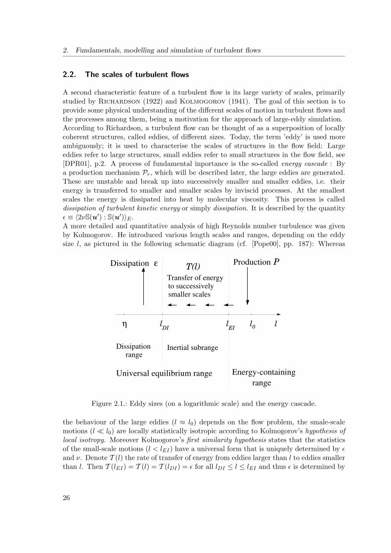
A second characteristic feature of a turbulent flow is its large variety of scales, primarilystudied by Richardson (1922) and Kolmogorov (1941). The goal of this section is toprovide some physical understanding of the different scales of motion in turbulent flows andthe processes among them, being a motivation for the approach of large-eddy simulation.According to Richardson, a turbulent flow can be thought of as a superposition of locallycoherent structures, called eddies, of different sizes. Today, the term ’eddy’ is used moreambiguously; it is used to characterise the scales of structures in the flow field: Largeeddies refer to large structures, small eddies refer to small structures in the flow field, see[DPR01], p.2. A process of fundamental inportance is the so-called energy cascade : Bya production mechanism Pr, which will be described later, the large eddies are generated.These are unstable and break up into successively smaller and smaller eddies, i.e. theirenergy is transferred to smaller and smaller scales by inviscid processes. At the smallestscales the energy is dissipated into heat by molecular viscosity. This process is calleddissipation of turbulent kinetic energy or simply dissipation. It is described by the quantityε ≡ 〈2νS(u′) : S(u′)〉E .A more detailed and quantitative analysis of high Reynolds number turbulence was givenby Kolmogorov. He introduced various length scales and ranges, depending on the eddysize l, as pictured in the following schematic diagram (cf. [Pope00], pp. 187): Whereas

ProductionDissipation

Energy-containingrange

Universal equilibrium range

η

Dissipationrange

Inertial subrange

llllEIDI 0

P

Transfer of energyto successivelysmaller scales

T(l)ε

Figure 2.1.: Eddy sizes (on a logarithmic scale) and the energy cascade.

the behaviour of the large eddies (l ≈ l0) depends on the flow problem, the smale-scalemotions (l l0) are locally statistically isotropic according to Kolmogorov’s hypothesis oflocal isotropy. Moreover Kolmogorov’s first similarity hypothesis states that the statisticsof the small-scale motions (l < lEI) have a universal form that is uniquely determined by εand ν. Denote T (l) the rate of transfer of energy from eddies larger than l to eddies smallerthan l. Then T (lEI) = T (l) = T (lDI) = ε for all lDI ≤ l ≤ lEI and thus ε is determined by

26

2.3. Criteria for appraising approaches in CFD

the transfer of energy from the largest eddies. Kolmogorov’s second similarity hypothesissays that in the inertial subrange the statistics depend only on ε.The characteristic lengthscale in the dissipation range is the so-called Kolmogorov scaleη = (ν3/ε)1/4. Then the ratio of the largest to smallest scales is of order Re3/4, whichdemonstates the vast range of scales.The question is how turbulent kinetic energy and dissipation are distributed among theeddies of different sizes. Denote κ = 2π/l the wavenumber corresponding to motions oflengthscale l. Then energy and dissipation in the wavenumber range (κa, κb) are given by

k(κa,κb) =∫ κb

κa

E(κ)dκ , ε(κa,κb) =∫ κb

κa

2νκ2E(κ)dκ ,

with E(κ) = E(κ, t) in statistically stationary turbulence and the energy spectrum functionE(κ, t) being defined in (2.4). By Kolmogorov’s first hypothesis, in the universal equilibriumrange (κ > 2π/lEI), E(κ) is a universal function of ε and ν. In 2π/lDI > κ > 2π/lEI thespectrum is given by

E(κ) = Cε2/3κ−5/3

with a universal constant C = 1.5, see [Pope00], p.231. Abundant physical experimentsconfirm this law.To answer the remaining question, the cumulative kinetic energy and the cumulative dissi-pation have to be introduced

k(0,κ) =∫ κ

0E(κ′)dκ′ ε(0,κ) =

∫ κ

02νκ′2E(κ′)dκ′ .

Since ε(0,2π/(60η)) = 0.1ε, significant dissipation occurs only for l ≤ 60η. Therefore thedemarcation lengthscale between the inertial and dissipative ranges is taken to be lDI =60η. Concerning the kinetic energy, if lEI = 1/6L11 and κEI = 2π/lEI , cf. (2.5), thenk(0,κEI) = 0.8k, i.e. eddies of size l > lEI contain 80% of the kinetic energy, cf. [Pope00],p.237 and p.241. For this reason, l > lEI is called energy containing range. Thus the bulkof kinetic energy is contained in the large-scale motions, whereas the bulk of dissipationaffects the small-scale motions.

2.3. Criteria for appraising approaches in CFD

Pope resumes the following criteria for appraising approaches in CFD, see [Pope00], pp.336,viz.,

• level of description,

• completeness,

• cost and ease of use,

• range of applicability,

• accuracy.

27


The level of description specifies which information is provided by the solution of a com-putation. For example, from a LES we can extract the Reynolds stresses carried by thelarge scale motion, whereas from a RANS computation, the only quantities obtained aremean values. A model is called complete if there are no unclosed terms in its constituentequations. Both the k/ε model and the LES models studied in this thesis are complete.The criterion concerning cost and ease of use of a model regards its use in a CFD code. Westart regarding the cost of a model. Firstly, we have to account for the number of operationsneeded to perform a computation. Secondly, we have to consider the memory consumptionof a computation. Clearly these two points dictate the scale of computer needed, i.e. asupercomputer or a workstation. There has been a tremendous progress in computer ar-chitecture in the last decades (see [HP96]). Moreover, the CFD community becomes moreand more aware of the need for architecture-friendly algorithms in order to exploit theimprovements in computer hardware, see e.g. the URL http://www.math.odu.edu/ keyes/and in particular [Key00]. Despite these efforts, a DNS for complex flows will be infeasibleeven with next decades supercomputers.One aspect of ease of use of a model concerns its numerical properties, e.g., its stability.A further point is regarding the post-processing required to extract the results of interest.In particular, a LES requires ensemble averaging whereas a RANS computation does not.Moreover, the model together with the numerical solution scheme impact the implementa-tion and the data structures required. This determines the ease of code implemention andmaintenance for a certain model. Fortunately, even in the CFD community, having reliedon Fortran and C for several decades, the trend is towards object-oriented programminglanguages. Using an object-oriented programming paradigm facilitates implementing andmaintaining complex CFD codes significantly without loss in performance, see e.g. theURL http://www.oonumerics.org/.Applicability concerns the question whether the model assumptions and requirements aresatisfied for a given flow problem. Finally, the accuracy of a model appraises the quality ofits predictions by comparison with experimental data.

28

3. The k/ε turbulence model

In the previous section we introduced the idea of reducing the complexity of a turbulentflow by a statistical approach. The objective of this chapter is to present the so-calledk/ε turbulence model. It is the most widely used statistical turbulence model, being in-corporated in most commercial CFD codes. The focus will be on the underlying modelapproximations with emphasis being placed on effects of buoyancy.

3.1. The Reynolds averaged Navier-Stokes equations

The starting point is the so-called Reynolds decomposition, cf. (2.1)

(u, p) = (〈u〉E , 〈p〉E) + (u′, p′) , θ = 〈θ〉E + θ′ ,

where 〈·〉E again denotes the ensemble averaging filter, defined in (2.2). For simplicity, inthe sequel, ensemble averaged quantities are designated by capital letters. Applying theensemble-averaging filter to the evolution equations in model TNSE yields the so-calledReynolds averaged Navier-Stokes equations (abbreviated RANS equations)

∂tU + (U · ∇)U +∇P −∇ · (2νS(U)− 〈u′ ⊗ u′〉E) = − βΘg ,(3.1)∇ ·U = 0 ,(3.2)

∂tΘ + (U∇)Θ−∇ · (a∇Θ− 〈u′θ′〉E) =qV

cp.(3.3)

These are ”nearly” the non-isothermal Navier-Stokes equations for the mean values ofvelocity, pressure and temperature. However, they contain two additional terms of crucialimportance. Therein, the velocity covariances 〈u′ ⊗ u′〉E appearing in the momentumequation are referred to as Reynolds stresses. They can be interpreted as additional stressesarising from the mean momentum flux due to the fluctuating velocity field. The analogousterm in the temperature equation, viz, 〈u′θ′〉, is called scalar flux. It describes the flux oftemperature due to the fluctuating velocity field. Pope generalises and emphasises thisobservation: In turbulent flows, the rates of mixing of momentum, heat and mass aregreatly enhanced, see [Pope00], p.7.Both fluctuation terms are functions of unknown correlations that cannot be expressed interms of mean quantities: Because of the non-linearity of the Navier-Stokes equations, thefirst moment equation contains second moments, the second moment equations will containthird moments, and so forth. Thus, to handle these terms, closure hypotheses are needed.

29


3.2. Turbulent-viscosity and gradient-diffusion hypotheses

3.2.1. The RANS equations using the turbulent-viscosity and gradient-diffusionhypotheses

In 1877, Boussinesq proposed the so-called eddy-viscosity hypothesis or turbulent-viscosityhypothesis. It assumes the constitutive relation

〈u′ ⊗ u′〉 = − 2νt S(U) +23kI ,(3.4)

where the positive scalar field νt is the so-called eddy-viscosity or turbulent viscosity. Some-times −〈u′⊗u′〉+ 2

3kI will be referred to as anisotropic Reynolds-stress. The second righthand side term in (3.4) is a normal stress correction which ensures that the traces of bothsides equal.Similarly the gradient-diffusion hypothesis assumes that

〈u′θ′〉 = − at∇Θ ,(3.5)

where at is the turbulent thermal diffusivity. Moreover we introduce effective viscosity νeand effective diffusivity at, viz,

νe = ν + νt , ae = a + at .(3.6)

Using (3.4), (3.5) and (3.6), the non-isothermal RANS equations (3.1)-(3.3) become

∂tU + (U · ∇)U +∇(P +23k)−∇ · (2νeS(U)) = − βΘg ,(3.7)

∇ ·U = 0 ,(3.8)

∂tΘ + (U∇)Θ−∇ · (ae∇Θ) =qV

cp.(3.9)

Here we should point out a further difficulty. We have two possibilities for treating theterm 2

3∇k arising in (3.4). We could (i) include it in the pressure term or we could (ii)modify the right hand side

(i) P ∗ ≡ P +23k , or (ii) f∗ ≡ f − 2

3∇k.

Case (i) is based on the observation that the stresses due to the term 23kI are normal

stresses that act like pressure forces. But it has the major disadvantage that when using p∗

as the independent pressure variable, special care must be taken when prescribing boundaryconditions involving the physical pressure, cf. [HC01], p.43.On the other hand, in case (ii) the right hand side is disturbed. In our field of interest, thestudy of indoor-air movement, the flow is induced and influenced by temperature differencesin a sensitive manner. Consequently we want to avoid contamination of this term by otherterms. In our research group therefore strategy (i) was chosen.The notion that the turbulent motion mixes both momentum and temperature motivates

30

3.2. Turbulent-viscosity and gradient-diffusion hypotheses

the goal to formulate a relationship between the turbulent heat flux and the Reynoldsstress tensor which is responsible for that flux. The simplest model is to assume that thescalar flux behaves analogously to the momentum flux. An immediate consequence of thisassumption is that there is a constant of proportionality, called turbulent Prandtl number,such that at = Pr−1

t νt, which can be rearranged to the more convenient form

Prt =νtat.(3.10)

Remark 3.1Prt can depend on many factors that influence the flow field. In particular, Prt is nota constant material property. In indoor-air flow problems, our research group choosesPrt = 0.9 remote from walls and Prt = 1.15 in the near-wall region, Prt being smoothin-between. This choice is in agreement with [PS01]. [DPR01], p.53 report Prt = 0.9in boundary layers and Prt = 0.7 in free-shear flows. This again reveals the problem inturbulence modelling that model constants are not physical constants. ♦

So far the closure problem for (3.1)-(3.3) has been reduced to the task of specifying thescalar field νt. This will be the objective of Section 3.4.

3.2.2. An appraisal of the turbulent-viscosity hypothesis

A thorough appraisal of the turbulent-viscosity and gradient-diffusion hypothesis can befound in [Pope00], Section 4.4 and Section 10.1, and in [Wilcox98], Section 3.2 and Chap-ter 6. According to Pope, the turbulent-viscosity hypothesis can be viewed in two parts,viz., an intrinsic part and a specific part. The intrinsic assumption is that the anisotropicReynolds-stress a ≡ 〈u′ ⊗ u′〉E − 2

3kI at each space-time point (x, t) is determined by thevalue of the mean rate-of-strain tensor at that space-time point (x, t), i.e., we assume thata(x, t) = f(S(U)(x, t)) with some function f . The specific assumption is to assume alinear relation.Obviously, turbulent-viscosity and gradient-diffusion hypothesis are analogous to Fourier’slaw and Fick’s law of molecular processes. Wilcox explains why the viscous stress term2νS(U) describes the momentum transfer at the molecular level and that ν is given by

ν =12vthlmfp ,(3.11)

where vth is the thermal velocity and lmfp is the mean free path, cf. [Wilcox98]. However,a consideration of the corresponding timescales shows that turbulent processes differ vastlyfrom molecular processes. The timescales corresponding to shear stress and turbulence areS−1 and k/ε, resp. The ratio of the molecular timescale to S−1 is very small (e.g. 10−10).Therefore molecular motion adjusts instantaneously to changes in mean straining. But ingeneral, turbulence does not adjust rapidly, because typically Sk/ε > 1.

Originally, the turbulent-viscosity hypothesis was used with an algebraic model for νt byPrandtl to describe simple shear flows like free-shear flows, e.g., the far wake or the

31


mixing-layer, and attached boundary-layer flows, see [Wilcox98], Chapter 3. Surprisingly,using a more sophisticated formula for νt, complicated two-dimensional flows can also bepredicted quite well. The Spalart-Allmaras model is a one-equation model conceived foraerodynamic applications, which predicts transonic flows over airfoils including boundary-layer separation successfully. Durbin developed the k − ε − v2 model, a successor of thestandard k/ε model, which has been applied successfully to complicated two-dimensionalflows like jet impingement.However, there are some situations where all models based on the turbulent-viscosity hy-pothesis fail inevitably: (i) Flows in ducts where the anisotropy of the Reynolds stressesgenerates a new component of the mean flow (often referred to as secondary motion), (ii)flows over curved surfaces and flows in rotating fluids and (iii) flows with sudden changesin mean strain rate. Describing the physics of (i), (ii) and (iii) correctly requires morecomplex models for the Reynolds stresses.

x

xx

1

2

333 S

S

Straight sectionAxisymmetric contraction

Straight section

ij

ij S22

Turbulencegridgenerating

S = S

= S = - 0.5S

= 0

= 011

λ

λ

Figure 3.1.: Sketch of Tucker-Reynolds flow experiment.

Ad (i): In order to predict the anisotropy of the normal Reynolds stresses, non-linearconstitutive relations (instead of the specific linear assumption a = νtS(U)) have beenproposed, see [Wilcox98], Chapter 6.2 and references therein.Ad (ii): In some situations, the individual components of the Reynolds stress tensor areaffected differently by the production of turbulence. For example, in flows over surfaceswith convex curvature the component directed toward the centre of curvature will be dimin-ished. Thus a further step is to solve an algebraic equation for the Reynolds stress tensor.Such an equation can be derived from the exact (but unclosed) partial differential equationfor the Reynolds stress tensor using some approximations for the unclosed terms and theterms including derivatives of the Reynolds stresses. This approach was originally devisedby Rodi and is explained e.g. in [Pope00], pp.448 and [Wilcox98] pp. 282. These so-calledalgebraic stress models provide a significant improvement for flows with mean streamlinecurvature.Ad (iii): On a statistical level, the most complete approach is to consider the partial dif-ferential equation for the Reynolds stress tensor. Closure models for unclosed terms lead

32

3.3. Production and dissipation of turbulent kinetic energy in RANS models

to Reynolds stress models, also called second moment closure models or Reynolds stresstransport models. An investigation of the resulting equation in the limit ||S(U)|| → ∞reveals that the evolution of the Reynolds stresses at time t depends on the prior historyof straining

∫ t0 ||S(U)||dt′ (Crow 1968), see [Pope00], p.405. This is in contrast to the

intrinsic assumption a(x, t) = f(S(U)(x, t)). For example, consider the experiment byTucker and Reynolds, sketched in Figure 3.1. When the strain is suddenly removed afterthe axisymmetrical contraction, the intrinsic assumption predicts zero Reynolds stresses.This is in contrast to the experimentally observed relatively slow return to isotropy of theReynolds stresses, see e.g. [Wilcox98], pp.274, and [Pope00], pp.359.As a final remark, it is quite interesting that in natural convection boundary layers theturbulent-viscosity hypothesis does not hold in the near-wall region, but the gradient-diffusion hypothesis is satisfied reasonably, see [TN98b].

3.3. Production and dissipation of turbulent kinetic energy in RANS models

3.3.1. Isothermal turbulent flows

This section is devoted to the processes in turbulent flows that generate and dissipateturbulent kinetic energy. First we consider the isothermal case. The kinetic energy of thefluid per unit mass is E(x, t) = u(x, t) · u(x, t)/2. We can decompose 〈E(x, t)〉E intothe kinetic energy of the mean flow E = U · U/2 and into the turbulent kinetic energyk = 〈u′ ·u′〉E/2. Starting from the RANS equations (3.1)-(3.2) and from the correspondingequation for u′, the following equations can be derived, cf. eq. (5.131)-(5.132) in [Pope00].

∂tE +U · ∇E +∇ ·(〈u′ ⊗ u′〉EU +UP − 2νS(U)U

)= − Pk − ε ,(3.12)

∂tk +U · ∇k +∇ ·(〈u′ ⊗ u′u′〉E + 〈u′p〉E − 2ν〈S(u′)u′〉E

)= Pk − ε ,(3.13)

with

ε ≡ 2νS(U) : S(U) , (dissipation due to the mean flow),(3.14)ε ≡ 2ν〈S(u′) : S(u′)〉E , (dissipation due to turbulent fluctuations),(3.15)Pk ≡ − 〈u′ ⊗ u′〉E : S(U) , (production of turbulent kinetic energy).(3.16)

The last term on the left hand side, i.e. ∇· (. . .), in (3.12)-(3.13) is called flux of energy, asit represents the transfer of mean flow kinetic energy resp. turbulent kinetic energy fromone region to another. Pk is a sink term in the equation for E and a source term in the kequation. Pk describes how kinetic energy is removed from the mean flow and transferredto the fluctuating velocity field. Using the turbulent-viscosity hypothesis, (3.16) becomes

Pk = 2νtS(U) : S(U) .(3.17)

3.3.2. Coupling between buoyancy and turbulence generation

Now we consider the case of buoyancy driven flows. Then we have to distinguish betweentwo phenomena:

(I) The stabilising effect of stratification.

33


(II) A (speculative) additional turbulence generation mechanism due to buoyancy as sug-gested by the theory of baroclinic vorticity generation.

First we study the effect of stratification on turbulence. In the non-isothermal case, equa-tions for E and k can be derived similar to (3.12)-(3.13), see e.g. [DPR01], pp.223. Thedifference w.r.t. (3.12)-(3.13) is that we have to replace Pk by Pk + G. G is often calledgravitational production term and is given by

G = − βd∑i=1

gi 〈uiθ〉E .(3.18)

It is convenient to define the flux Richardson number

Rif ≡−GPk

,(3.19)

which is a measure for the stabilising effect of stratification. If Rif > 0, then turbulence issuppressed; if Rif < 0, then turbulence is enhanced.Regarding (II), at the present stage of knowledge, there are two concurring theories regard-ing an additional coupling mechanism between buoyancy and turbulence generation, beingreported briefly by Tieszen et al. in [TODB98].First both perspectives will be reviewed. According to the more traditional theory, the onlyeffect of buoyancy (i.e., density gradients) is to induce vertical momentum. Ascending airrequires a transverse inflow. Then turbulence is only due to large-scale instabilities (meanvelocity gradients) and the subsequent turbulent energy cascade. The second perspectiveviews buoyancy in terms of the so-called baroclinic vorticity generation (BVG): In a gravi-tational field, temperature gradients perpendicular (normal) to the direction of gravity tendto result in the generation of vorticity, also referred to as small-scale instabilities. Thesevortical structures randomly interact with themselves and with the existing turbulence.Having presented both viewpoints, Tieszen et al. draw the following conclusions re-garding the modelling of an additional buoyancy-turbulence interaction. Regarding thetraditional perspective, buoyancy acts only on the large lengthscales. In this case, there isno need for modifying the turbulence model under consideration. On the other hand, theBVG theory says that there is an additional interaction between buoyancy and turbulencethat has to be modelled.A relevant situation concerning (II) is a flow along a vertical hot wall. Then in the near-wall region vertical stratification is small compared to the large temperature gradients incross-stream direction. The observation that the turbulent-viscosity hypothesis does nothold in the near-wall region can be viewed as an indication of the BVG-hypothesis, see[TN98b].

3.4. A two-equation model : The k/ε model

3.4.1. The k/ε model for buoyancy driven flows

Two-equation models are based on the so-called Kolmogorov-Prandtl relation

νt = cu∗lm , with u∗ = cu∗k1/2 .(3.20)

34


(3.20) can be regarded as a formal analogy to (3.11). lm and u∗ are a suitable lengthscaleresp. a suitable velocity scale, being a formal analogy to lmfp and vth resp. in (3.11). Usingdimensional analysis, lm can be expressed using k and ε according to

lm = clmk3/2ε−1 .(3.21)

Combining (3.20) and (3.21) we can compute νt from k and ε using the formula

νt = Cµk2

ε, Cµ = 0.09.(3.22)

Here the value Cµ = 0.09 is chosen to ensure a correct behaviour in shear flows.In the k/ε model, k and ε are obtained as solutions of partial differential equations; conse-quently the model will be finally closed. Using the closure approximation

(〈u′ ⊗ u′u′〉E + 〈u′p〉E − 2ν〈S(u′)u′〉E = − νtPrk∇k ,(3.23)

in (3.13), the following equation for k is obtained (using the further approximation thatPrk = 1.0 equals a constant)

∂tk + (u ·∇)k −∇ · ( νtPrk∇k) = Pk − ε .(3.24)

Compared to the k equation, the equation for ε ”is best viewed as being entirely empirical”([Pope00], p.375); it reads (with constants Prε, C1, C2 being specified later)

∂tε+ (u ·∇)ε−∇ · ( νtPrε∇ε) + C2ε

2k−1 = C1εk−1Pk .(3.25)

An attempt to a mathematical approach to (3.24) and (3.25) can be found in [MP94].The standard modification of the k/ε model for buoyancy driven flows is based on simplyreplacing Pk with Pk + G, being defined in (3.16) resp. (3.18). Then for Pk and Gthe turbulent-viscosity resp. gradient-diffusion assumptions are used. This was originallydevised by Ince and Launder, see [IL89], who proposed to replace Pk by

Pk +G , with G ≡ CtβνtPrt

g · ∇Θ , Ct = 0.8 .(3.26)

However, (3.26) can only describe the interaction between stratification and turbulence, seeSubsection 3.3. As pointed out in [TODB98], p. 294, (3.26) cannot describe the followingphenomenon. In a flow along a vertical hot wall, the vertical stratification is small comparedto the temperature cross-stream gradient. On the one hand, formula (3.26) implies G = 0as temperature gradients are perpendicular to the direction of gravity. On the other hand,BVG theory says that temperature gradients perpendicular to the direction of gravity tendto result in the generation of vorticity. Therefore [TODB98] emphasise using the so-calledgeneralized gradient-diffusion hypothesis, originated by Daly and Harlow (1970), see[DH70], and applied by Ince and Launder, cf. [IL89], viz.,

G = − βcθk

ε

d∑i,j=1

gi

[23kδij − νt

(∂Ui∂xj

+∂Uj∂xi

) ]∂Θ∂xj

(3.27)

35


with constant cθ with standard value cθ = 0.18. Numerical tests with our research coderevealed that (3.26) and (3.27) give almost the same results due to our near-wall modellingstrategy. However, when resolving the near-wall region, (3.27) is reported to be superior to(3.26), see [TODB98]. Thus, for practical reasons, we use (3.26). To this end, using (3.26)we arrive at the following system of equations for U , P , Θ, k and ε

∂tU −∇ · (2νeS(U)) + (U ·∇)U +∇P = − βΘg(3.28)∇ ·U = 0(3.29)

∂tΘ + (U ·∇)Θ−∇ · (ae∇Θ) = qV c−1p(3.30)

∂tk + (U ·∇)k −∇ · (νk∇k) = Pk +G− ε(3.31)

∂tε+ (U ·∇)ε−∇ · (νε∇ε) + C2ε2k−1 = C1εk

−1(Pk +G)(3.32)

with turbulent-viscosity and thermal diffusivity being related by the turbulent Prandtlnumber

νt = Cµk2

ε, a = νPr−1 , at = νtPr

−1t ,with Pr = 0.70 , P rt = 0.9 for air,

(3.33)

with effective viscosities

νe = ν + νt , ae = a+ at , νk = ν +νtPrk

, νε = ν +νtPrε

(3.34)

and with experimentally determined constants (see below)

C1 = 1.44 , C2 = 1.92 , P rk = 1.0 , P rε = 1.3 , Ct = 0.8 , Cµ = 0.09,(3.35)

Production and buoyancy terms Pk and G are defined in (3.17) and (3.26).It is not possible to determine the empirical constants of the k/ε model from a set ofmeasurements that isolate each term, because the model is not exact. The standard valuesare rather a compromise for a range of flows. Nevertheless it is worth mentioning that C2

determines the decay of homogeneous, isotropic turbulence. The spreading rate of shearlayers is controlled by C2 − C1. Boundary-layer data suggest C1 = 1.55, whereas C1 = 1.3is appropriately for mixing layer data, see [DPR01], p.181. Discernibly the standard valueC1 = 1.44 is a compromise.

3.4.2. An appraisal of the k/ε model

A principal limitation of the the k/ε model arises from the underlying turbulent-viscosityhypothesis and its formula for νt. Instead of the full Reynolds stress tensor only half itstrace k is computed. Moreover, in Wilcox’s opinion, the closure approximation (3.23)for the k-equation and much more notably those for the ε equation (given in [Wilcox98]eq.(4.45)), are a ”drastic surgery” on the exact equations. Whereas turbulent-viscosity andgradient-diffusion hypotheses have been investigated using various experimental data, the

36


terms modeled in the k and ε equation are almost impossible to measure. However, thereis hope that DNS studies can help to gain information for suitable closure approximations.A further dispute is on the question whether the lengthscale provided by ε is the correctone for (3.20). For more details, the reader is addressed to [Pope00], Section 10.4 and[Wilcox98], Subsection 4.3.2.The values of the constants in (3.35) are a compromise, balanced for several basic testcases, e.g. decaying turbulence and behaviour in the log-layer. The standard k/ε modelyields acceptable results for the mixing layer and for the plane and radial jet, cf. [Wilcox98]pp.137. However, the k/ε model erroneously predicts unequal rates for spreading for roundand plane jets, a phenomenon referred to as ’round jet-plane jet anomaly’. Of course,the constants can be tuned for a particular flow. It is noteworthy that values for themodel constants can be derived from renormalization group (RNG) analysis. Despite itsmathematical reasoning, in practice this does not provide a significant improvement to thestandard k/ε model, cf. [Wilcox98], p.137.The main deficiencies of the k/ε model are its poor predictions (i) in the near-wall regionand (ii) for flows with strong pressure gradients. The latter is discussed in great detail in[Wilcox98], Chapter 4.6.2. As pointed out in [DPR01], Section 6.2.2, the behaviour of thek/ε model below the log-layer imposes several severe difficulties. First it is not a trivialtask to specify meaningful boundary conditions for ε at solid walls. Secondly, in (3.25) theterm C2ε

2/k behaves like y−2 near the wall, with y denoting the distance from the wall,and hence becomes singular. Finally, even if the exact data for k and ε (e.g. from a DNSdata base) are substituted into νt = Cµk

2/ε, the theoretical value νt ≡ −〈u′v′〉E/(dU/dy)is spuriously overpredicted close to the wall.These problems gave rise to several of modifications of the k/ε model near solid walls, mostnoteworthy (a) low Reynolds number models, (b) wall functions (c) two-layer models, (d)the k-ε-v2 model by Durbin, for details see [DPR01], Chapter 6.2.2 and references therein.Low Reynolds number models introduce artificial damping functions for damping νt nearthe wall. They are unreliable for flows with significant pressure gradient and cause numer-ical stiffness problems. Hence this approach is virtually unanimously doomed in the CFDcommunity. Approach (b) has been employed in our research group and will be describedin great detail in this thesis. It is computationally attractive since it circumvents resolvingthe near wall region. The wall function concept can be justified for attached boundary-layerflows with small pressure gradients. In practical applications wall functions are also usedwhen the underlying assumptions do not hold. In flows with massive separation or strongpressure gradients their predictions can be poor. However, such situations do not oftenoccur in indoor-air flow problems. Nevertheless, more accurate approaches are desirable.The strategies (c) and (d) both require a near-wall grid. A two-layer model was devisedby Chen and Patel, who proposed to use a suitable one-equation model for k in thenear-wall region, which is matched with the k/ε model at a certain artificial boundary inthe log-layer.The k-ε-v2 model is a four equation model, presented in [Dur91]. It is based on the ideathat it is the cross-stream fluctuation velocity v′2 that is responsible for turbulent mo-mentum transport in the near-wall region and that v′2 is suppressed in the proximity ofwalls. The model adds one advection-diffusion-reaction equation for the scalar v2 and an

37


advection-reaction equation for a scalar f which is motivated from the theory of secondmoment closure modelling and tries to emulate effects of redistribution of turbulent kineticenergy from the streamwise to the wall-normal component. Very reasonable results havebeen obtained even for complicated test cases including separation and jet impingement,see [DPR01]. The notion that the model k-ε-v2 model is significantly superior to the k/εmodel in predicting the heat transfer in an axisymmetric turbulent jet impinging on aflat plate, [BPD98], makes this model quite attractive for application in indoor-air flowproblems. It is worth mentioning that Piomelli et al., see [SP02] performed a thor-ough study of today’s most successful near-wall RANS models, including the one-equationSpalart-Allmaras model, the k/ε model with the wall functions of Lam and Bremhorst,the k/ω2 model of Saffman and Wilcox, and the k-ε-v2 model of Durbin for a pulsatingflow in [SP02], the latter being the most successful.Besides the k/ε model, there are other two-equation models, most remarkebly the k/ωmodel. It has two well-known advantages over the standard k/ε model. First, it yieldsreasonable predictions for the mean velocity field throughout the near-wall region provideda suitable near-wall grid is used. Secondly, it gives good results even for flows with strongpressure gradients. Both observations have made this model very interesting for aeronauti-cal flows. However, a more detailed analysis reveals that the propitous predictions for νt arejust a consequence of underpredicting k and overpredicting ε; its success in the near-wallregion is not based on physical reasoning. Moreover the model is unreliable for free-shearlayers, whose correct predictions are also quite important for indoor-air flow problems, see[DPR01], p.132. Thus concerning future projects, the k-ε-v2 model seems to be the mostpromising RANS model for problems involving indoor-air movement.

38

4. Large-eddy simulation

This chapter is dedicated to large-eddy simulation (LES). LES is an alternative approach forreducing the complexity of turbulent flow problems. As described in Section 2.2, turbulentflows are characterized by a large range of scales, the ratio of the smallest to largest eddiesincreasing as Re−3/4. When the turbulent motions of all scales are fully resolved, i.e. ina DNS, the computational efforts for resolving the small scale motions exceed those forresolving the large scale motions by far. Since engineers are primarily interested in thebehaviour of the large scale motions, ”there is a mismatch between DNS and the objectiveof determining the mean velocity and energy-containing motions in a turbulent flow”, aspointed out by [Pope00], p.357. Thus the idea is to reduce complexity of turbulence by firstfiltering out the small scale motions using a spatial filter, resolving the random motion ofthe remaining large eddies. However, again a closure problem arises. Thus the idea of LESis to resolve the large-scale motions and to model the effects of the small-scale motions onthe large-scale motions. This approach is supported by the observation that the small-scalemotions have, to some extent, a universal behaviour, making them amenable for modelling.

4.1. Filtering

The objective of filtering a variable is to extract its large-scale structures and to attenuateits small-scale structures. The filter width ∆ specifies the demarcation line of this scaleseparation. Such a space-averaging filter 〈·〉∆ should have the following properties:

(F1) Filtering is a linear operation, i.e. 〈f + λg〉∆ = 〈f〉∆ + λ〈g〉∆ , f, g : Rd → R, λ ∈ R.

(F2) Derivatives and averages commute, i.e. 〈 ∂f∂xi 〉∆ = ∂〈f〉∆∂xi

, 〈∂f∂t 〉∆ = ∂〈f〉∆∂t .

The classical filtering technique used in LES is the convolution with a suitable filter func-tion. Let f(x, t) be an instantaneous variable. If f is defined w.r.t. the spatial variable ona bounded domain Ω, then f is extended by zero onto Rd. Then its corresponding filteredvariable is defined by the convolution integral

f(x, t) ≡ 〈f〉∆ =∫Rd

g∆(x− y)f(y, t)dy, g∆(x) =d∏j=1

gj∆(xj) .(4.1)

with g∆ being a filter function and ∆ denoting the filter width. If f is vector-valued resp.tensor-valued, then filtering has to be understood componentwise. Since f ≡ 0 on Rd \ Ω,f ∈ E ′ ⊂ S ′, cf. Section A.1. Given g∆ ∈ S, the spatial averaging filter can be interpretedas an operator 〈·〉∆

〈·〉∆ : S ′(Rd) 7→ S(Rd), 〈f〉∆ ≡ g∆ ∗ f .(4.2)

39


If ∆ = const, then the filter defined by (4.1) satisfies (F1) and (F2), see Theorem A.4.f(x, t) is the weighted mean value of f with weight function g∆(x − ·). In the casesupp(gj∆) ⊂ [−∆,∆] the averaging is performed over B∆(x) (ball in the maximum norm).Then velocity, pressure and temperature can be decomposed into a filtered part and aresidual part, videlicet,

(u, p)(x, t) = (u, p)(x, t) + (u′, p′)(x, t) , (u′, p′)(x, t) ≡ (u, p)(x, t)− (u, p)(x, t)(4.3)

θ(x, t) = θ(x, t) + θ′(x, t) , θ′(x, t) ≡ θ(x, t)− θ(x, t)(4.4)

It is worth considering the effect of the filtering operation in the Fourier space. The relation

f ≡ F(f) = F(g∆ ∗ f) = F(g∆)F(f).(4.5)

shows that all the high wave number components of f are annihilated by convolution withg∆, if F(g∆)(κ) = 0 for |κ| > κc, where κc is a cut-off wave number. A filter with such acharacteristic is called an ideal low pass filter. If the filter function in wave number spacerapidly falls off, a cut-off wave number can also be defined for all practical purposes.

The most popular filtering functions in LES and their corresponding Fourier transformsare, cf. [Pope00], p.563:

1. Box filter

gj∆(xj) =

1∆ , if |xj | ≤ ∆/20, if |xj | > ∆/2.

, gj∆(kj) =sin(∆kj/2)

∆kj/2,(4.6)

2. Sharp spectral filter

gj∆(xj) =sin(πxj/∆)

πxjgj∆(kj) =

1, if |kj | ≤ π/∆0, if |kj | > π/∆.

,(4.7)

3. Gaussian filter

gj∆(xj) =√

γ

π∆2e−

γx2j

∆2 , gj∆(kj) = e−

∆2k2j

4γ , γ = 6 .(4.8)

The specification γ = 6 in (4.8) ensures that box filter function and the Gaussian have thesame second moment, see [Pope00], p.563. Direct calculation yields the following equationsfor u′, cf. [Pope00], p.566,

u′(κ, t) ≡ F(u′)(κ, t) = [1− g∆(κ)]u(κ, t) , u′(x, t) = u(x, t)− u(x, t)(4.9)

On the one hand, the Gaussian is reasonably sharp both in physical space and in wavenum-ber space, see (4.8). On the other hand, since 0 < g∆(x) ≤ 1 and 0 < g∆(κ) ≤ 1 it follows

40

4.2. Differential filtering

that, in principle, filtering with a Gaussian is an invertible operation (although poorlyconditioned).It is worthwhile studying the resolution requirements for the filtered field. Denote κc = π/∆the cutoff wavenumber. For the Gaussian u(κ, t) = g∆(κ)u(κ, t) > 0 (for κ > κc), i.e.despite filtering, u(κ, t) has a non-vanishing contribution for κ > κc. Equivalently spoken,u contains (non-negligible) structures of size smaller than ∆. This suggests to resolve u upto κr , called the highest resolved mode, with κr = nκc (n ≥ 2). In other words, filter width∆ and the grid size of a numerical calculation h should be related by ∆ = nh (n ≥ 2). Thisintuitive reasoning is supported by numerical analysis, cf. [JL01].

4.2. Differential filtering

Explicit filtering is an important issue in LES. In the previous section, filtering was intro-duced using an integral operator, viz.,

u(t,x) = (g∆ ∗ u0)(t,x) , g∆(y) =( γ

π∆2

)d/2exp(−γy

2

∆2) .(4.10)

In his work on differential filters, Germano proposed to approximate this type of integraloperator by taking the inverse of an appropriate differential operator, cf. [Ger86]. Inthe appendix, this approach will be motivated by (A.25). The objective of this sectionis to describe the relation between the convolution with a gaussian filter and the solutionoperator of the heat equation. For this purpose we consider the Cauchy-problem of theheat equation: For given u0 ∈ S(Rd) find u : Rd × R+ 7→ R s.t.

∂u

∂s− a2∇2u = 0 in R

d × R+ ,(4.11)

u = u0 in Rd × 0 .(4.12)

Its solution u(x, s) is given by (cf. [Kre89], p.134)

u(x, s) = (G ∗ u0)(x, s) , G(y, s) = (4πa2s)−d/2 exp(−||y||

2

4a2s

),(4.13)

which holds even for u0 ∈ S ′(Rd). For s small, we can approximate the solution u(·, s) of(4.11)-(4.12) using one step of a backward Euler scheme. Using the notation u(·, 0) = u0,the solution u(·, s) of the problem

u(x, s)− u0(x)s

− a2∇2u(x, s) = 0 in Rd × R+(4.14)

is an approximation to the solution of (4.11)-(4.12). Thus, for fixed s, the solution of(−a2s∇2 + I

)u(x, s) = u0(x) in R

d × R+

is an approximation to u(·, s) in (4.13). Comparing (4.13) with (4.10) implies ∆2γ−1 =4a2s.

41


After this motivation we can describe how to approximate (4.10) using a differential filter:Given u(x, t) (t being fixed), approximate u(x, t) ≡ (g∆ ∗ u)(x, t) as solution us of(

−∆2

4γ∇2 + I

)us(·, t) = u(·, t) in R

d .

Often u(x, t) is given in Ω × R+ and Ω is a domain. Denote R(u) (a suggestion for) anapproximation of u(x, t). Then given u : Ω×R+ 7→ R, we seek R(u) : Ω×R+ 7→ R s.t. foreach fixed t (

−∆2

4γ∇2 + I

)R(u)(·, t) = u(·, t) in Ω, ∇R(u) · n = 0 on Γ .(4.15)

The idea of choosing a Neumann boundary condition in (4.15) is to keep the modelling errornear the boundary small.To the author’s best knowledge, error estimates of ||g∆∗u−R(u)||are not available. ||g∆ ∗ u−R(u)|| will be studied numerically in Section 12.3.

Remark 4.1An alternative differential filter based on the solution of a Stokes problem was proposed byLayton, see [LL03]. A further question is whether the differential filtering scheme can beimproved by using a higher order scheme w.r.t. the variable s in (4.11). ♦

4.3. The space averaged non-isothermal Navier-Stokes equations

This section is devoted to the evolution equations for u, p and θ and to the closure problemin non-isothermal LES. Assume u, p and θ are extended by zero onto Rd. Then applyinga spatial averaging filter 〈·〉∆ to (1.19)-(1.21) gives (using (F1) and (F2))

∂tu−∇ · ( 2 ν S(u)− u⊗ u+ u⊗ u ) + (u ·∇)u+∇p = − β θ g ,(4.16)∇ · u = 0 ,(4.17)

∂tθ + (u ·∇)θ −∇ ·(a∇θ − u θ + u θ

)= qV c−1

p .(4.18)

Remark 4.2Regarding the isothermal Navier-Stokes equations, we can assume the following regu-larities, cf. e.g. [Tem77]: f ∈ L2(0, T ; (H1

div(Ω)∗)d), u ∈ L2(0, T ; (H1div(Ω))d), ∂tu ∈

L1(0, T ; (H1div(Ω)∗)d), and ∇p ∈ E ′(Ω× (0, T )). Therefore, for each t ∈ (0, T ), ∇u and 4u

are at least in E ′(Ω) for each t ∈ (0, T ). Hence, for each t ∈ (0, T ), the expressions on bothsides are at least in S ′(Rd) and we can convolve both sides with a function g∆ ∈ S(Rd). ♦

Remark 4.3According to John and Layton, the extension of variables onto Rd leads to a commutationerror in the Navier-Stokes equations due to a loss in regularity. John and Dunca studiedthis error in the case of the isothermal Navier-Stokes equations with homogeneous Dirichletconditions. Extending u by zero in Rd \ Ω gives rise to an additional boundary term bothin the Navier-Stokes equations for u in Rd and the space filtered equations. However, in anumerical solution using FEM, this term is negligible small, cf. [Joh02], pp.10 and pp.14.

♦

42

4.3. The space averaged non-isothermal Navier-Stokes equations

It is worth emphasising that the fields involved in (4.16)-(4.18), i.e u, p, and θ are stillrandom.Equations (4.16)-(4.18) are unclosed. Similar to the RANS equations, we introduce

τR ≡ u⊗ u − u⊗ u , residual stress tensor ,(4.19)

kr ≡12

d∑i=1

τRii , residual kinetic energy ,(4.20)

τ r ≡ τR − 2dkrI , anisotropic residual stress tensor ,(4.21)

h ≡ u θ − u θ , residual temperature flux .(4.22)

The isotropic residual stress is included in the modified pressure pmod ≡ p + 2dkr. The

residual stress tensor and the residual temperature flux represent the effects of the residualscales on the filtered scales. They are often referred to as subgrid scale (abbreviated SGS)stresses and fluxes resp. Their modelling will be studied in Section 4.4.

As described in Section 2.2, the transfer of kinetic energy between filtered and residualscales is an important mechanism in turbulent flows. In order to quantify this, we focus onfiltered kinetic energy E(x, t), kinetic energy of the filtered velocity field Ef and residualkinetic energy kr, being defined as

E ≡ 12u · u , Ef ≡

12u · u , kr ≡

12u · u− 1

2u · u , with E = Ef + kr .(4.23)

Multiplying (4.16) with u we obtain the conservation equation for Ef , viz.,

∂tEf + u ∇Ef −∇ · [(2νS(u)− τ r − pI)u] = − εf − Pr − βθg · u ,(4.24)

where

εf ≡ 2νS(u) : S(u) , Pr ≡ −τ r : S(u) .(4.25)

The corresponding equation for kr reads (cf. e.g. [PYA96], p.217 or [Sag01], p.37)

∂tkr + u · ∇kr −∇ · [(E u− 12u · uu) + (p u− pu) + ν∇kr + τ ru]

= − εν + Pr − βθ′u′ · g(4.26)

with

εν ≡ ν

d∑i,j=1

∂ui∂xj

∂ui∂xj−

d∑i,j=1

∂ui∂xj

∂ui∂xj

.(4.27)

The right hand side terms in (4.24) and (4.26) are source or sink terms. εf describes viscousdissipation directly from the filtered velocity field, being small compared to ε, cf. [Pope00],p.588. εν represents the residual kinetic energy dissipated by viscous forces. Pr appears asa sink term in the equation for Ef and as a source term in the equation for kr. It representsthe rate of transfer of energy from the filtered velocity field to the residual motions. In themean, Pr > 0, but locally, backscatter can occur with Pr < 0, i.e. energy transfer from theresidual motions to the filtered motions.

43


4.4. Modelling the residual stress tensor and the residual fluxes

In order to close (4.16)-(4.18), we have to model τ r and h. Concerning the isothermalcase, for a survey on closure models see [Pope00], [Sag01] and [Geu01]. A mathematicalreview can be found in e.g. [Lay02] and [Lay02a]. For detailed numerical tests of the mostpopular residual stress models see e.g. [VGK97]. In subsection 4.4.1, we accomplish closuremodelling using formal series expansions, also referred to as structural modelling. We willaugment this with a functional model in order to explicitely account for the energy cascade,see subsection 4.4.2. Effects of buoyancy are regarded in subsection 4.4.3.

4.4.1. Structural modelling

One classical strategy for obtaining models for the residual stress tensor and the residualtemperature flux is so-called structural modelling: The underlying idea is to use formalseries expansions for the filter kernel in Fourier space. A detailed derivation of the followingtwo models can be found in appendix A.2. Starting point is the decomposition

u⊗ u = (u+ u′)⊗ (u+ u′) = u⊗ u+ u⊗ u′ + u′ ⊗ u+ u′ ⊗ u′(4.28)

θu = (θ + θ′)(u+ u′) = θ u+ θ u′ + θ′ u+ θ′ u′(4.29)

with resolved stresses resp. fluxes u⊗ u and θ u, cross stresses resp. fluxes u⊗ u′, u′ ⊗ u,θ u′ and θ′ u, and residual stresses resp. fluxes u′ ⊗ u′ and θ′ u′. We introduce

τSGS ≡ u′ ⊗ u′ − 1d

d∑i=1

u′ ⊗ u′) I , trace(A) ≡d∑i=1

Aii for A ∈ Rd×d ,(4.30)

hSGS ≡ u′θ′ .(4.31)

The so-called Clark model is based on a Taylor approximation of the filter kernel in Fourierspace. The Clark model reads

u⊗ u = u⊗ u +∆2

12∇u • ∇u + Oformal(∆4)

θu = θ u +∆2

12∇θ ∇u + Oformal(∆4)

with the notations

(∇U • ∇U)ij =d∑l=1

∂Ui∂xl

∂Uj∂xl

, (∇Θ ∇U)j =d∑l=1

∂Θ∂xl

∂Uj∂xl

.(4.32)

Instead, Galdi and Layton proposed using a rational approximation for the filteringkernel, leading to the following model

u⊗ u = u⊗ u +∆2

12R (∇u • ∇u) + Oformal(∆4)

θu = θ u +∆2

12R(∇θ ∇u

)+ Oformal(∆4)

with the regularization operator R defined in (4.15).

44


Remark 4.4There is an interesting formal connection between the Galdi-Layton model and today’smost successful Reynolds-stress model, the so-called elliptic relaxation model devised byDurbin, see [Dur93]. Both models use a similar elliptic regularization operator.

Remark 4.5The Fourier analysis reveals that the residual stress term and the residual flux term areof formal order ∆4 for both the Clark model and the Galdi-Layton model. Hence theircontribution is neglected in both models. Moreover, numerical tests show that for bothmodels the transfer of energy from the resolved scales to the residual scales is too smallleading to numerical instabilities for high Reynolds/Rayleigh numbers, see. e.g. [LMK94],[VGK97] and [Joh02]. For these reasons in the following subsection we introduce twoadditional subgrid scale models which are based on the turbulent-viscosity hypothesis. ♦

Remark 4.6The Galdi-Layton model has to be combined with a suitable damping function in order toobtain an appropriate near-wall behaviour. ♦

4.4.2. Functional modelling part I : Residual stress modelling for isothermal problems

The SGS models presented in this subsection are based on the turbulent-viscosity hypoth-esis. The objective of functional modelling is to provide a mechanism to transfer energyfrom the filtered scales to the residual scales and to dissipate energy at the end of theenergy cascade. As pointed out in [VGK97] this is an issue of major importance in LES.In analogy to Prandtl’s mixing length hypothesis (see (5.31)), Smagorinsky (1963)proposed

τ r = − 2νtS(u) , with νt ≡ (CS∆)2S , S ≡√S(u) : S(u) .(4.33)

From the relation Pr ≈ ε, Lilly (1967) obtained CS = 0.17.

Remark 4.7Another interpretation is to replace τ r by τSGS in (4.33). This interpretation accounts forthe fact that τSGS is formally of order ∆4 and is neglected in the structural modelling.However, the resulting effective model is the same.A fundamental problem of the Smagorinsky model concerns the choice of C2

S , which is ingeneral flow dependent. Lilly’s approach is reviewed in [BFR80]. Using a constant value forC2S might cause excessive dissipation, e.g. in turbulent channel flow and in the turbulent

mixing-layer, see [LMK94], [VGK97] and references therein. Moreover, in laminar (shear)flow CS must equal zero. In 1991, Germano devised a widespread modification of (4.33),cf. [GPMC91], viz., to compute CS in terms of the filtered velocity field. ♦

The Smagorinsky model can be viewed as a so-called turbulent kinetic energy (TKE) model.TKE models are based on the Kolmogorow-Prandtl relation (3.20) with lm = ∆ and u∗ ≈√kr. Here for u∗ a model for

√kr is needed. Note that for the Smagorinsky model applied

to high-Reynolds-number turbulence with the filter width in the inertial subrange the choicelm ∼ ∆ can be confirmed, cf. [Pope00], pp.587. The Smagorinsky model takes u∗ ∼ ∆S,

45


which can be viewed as an algebraic model for u∗.The Smagorinsky model is (formally) of second order in ∆, whereas the SGS term in Fourieranalysis is of fourth order in ∆. This is a mismatch (at least formally). Moreover, in manyflow experiments the Smagorinsky model has been turned out to be too dissipative - that is,it transfers too much energy to the residual motions. This motivates considering a furtherSGS model.Bardina (1980) suggested a different choice for u∗, based on the second identity in (4.9),cf. [BFR80], viz.,

u∗ = Cq|u · u− u · u|1/2 , with Cq = 0.126.

Similarly, Iliescu and Layton proposed

u∗ = Cq

√|u− u|2 ≈ Cq

√|u− u|2 = Cq|u− u| , with Cq = 0.17 ,

leading to the following model for νt:

νt = Cq∆|u− u| .(4.34)

The Iliescu-Layton model can be written as (see [IL98] eq. (2.6))

νt = Cq∆3

6||4u||2(4.35)

demonstrating that this model is formally of third order in ∆.

Remark 4.8An inherent problem of TKE models is that they are unable to give accurate predictionsfor τ r and Pr simultaneously. This stems from the fact that this type of model implies amuch too large correlation ρr between τ r and S(u). Measurements by Liu show ρr between0 and 0.2 (cf. [LMK94]). However, substituting e.g. the Smagorinsky model for τ r givesa value ρr ≈ 0.88 under some assumptions concerning the probability distribution of S(u),cf. [Pope00] exercise 13.33. Thus if the Smagorinsky coefficient chosen ensures a reason-able value for 〈Pr〉E , then the modelled residual stresses are significantly underpredicted,cf. [Pope00], p.603. This flaw is confirmed by numerical investigations, see e.g. [VGK97],section 3.2.4. But, as mentioned above, there is wide agreement that the correct predictionof Pr is much more important than the prediction of τ r.To ensure that the classical Smagorinsky model and the Iliescu Layton model behave rea-sonable near solid walls, νt has to be damped near the wall. For details see Chapter 7. Asa final remark, note that both models predict νt ≥ 0 and thus preclude backscattering. ♦

4.4.3. Functional modelling part II : SGS modelling for non-isothermal problems

First effects of buoyancy will be neglected. We focus on modelling the residual temperatureflux using the gradient-diffusion hypothesis with SGS diffusivity at, viz.,

h ≡ − θ u+ θu = − at∇θ .(4.36)

46


In analogy to the dynamic Smagorinsky model, the so-called dynamic scalar model usesat = Ca∆2S, with Ca being determined dynamically, see [PD98] and references therein. Analternative approach for specifying at is to relate at to νt by introducing a SGS turbulentPrandtl number Prt ≡ νta

−1t . A priori, Prt is an unknown scalar field which can be

determined dynamically. In this thesis we choose Prt = 0.4 remote from solid walls. Forthe treatment of Prt in the near-wall region see section 7.1.1. Further details are given inthe next subsection.

4.4.4. Functional modelling part III : SGS modelling for buoyancy driven problems

Now the effect of thermal stratification on residual stress modelling will be explored. Recallthat in the k/ε model, the production term is modified to account for effects of stratification,cf. (3.26). Via the production term Pk + G, gravitational production affects k and henceνt = Cµk

2/ε.Residual stress modelling for buoyant convection was investigated most remarkebly byLilly, see [Lil62], and Eidson, see [Eid85]. Eidson’s reasoning starts by assuming thatin buoyant convection the total transfer of energy from the filtered motions to the residualmotions is given by

Pθr ≡ − τ r : S(u) − βg · h .(4.37)

Equation (4.37) is motivated by Lilly’s analysis for the corresponding compressible case,cf. eq. (10)-(11) in [Lil62].Using the eddy-viscosity assumption τ r = −2νtS(u) implies that the transfer of energy fromthe resolved scales to the residual scales is predicted to be 2νtS. In the isothermal case, νthas to be chosen such that 2νtS is a reasonable approximation to Pr ≡ −τ r : S(u). Twoappropriate choices were discussed in subsection 4.4.2. In the case of buoyant convection,Lilly and later Eidson suggested to choose νt such that 2νtS is a suitable approximationto Pθr ≡ − τ r : S(u) − βg · h.

The Lilly-Eidson model

Based on the work of Lilly and Eidson, in [PD98] Peng and Davidson resume thefollowing modified choices for νt for buoyancy driven flows

1. Lilly-Eidson model

νt =

CE∆2

(S2 + β

Prtg · ∇θ

)1/2, if S2 ≥ − β

Prtg · ∇θ

0 , otherwise, at = Pr−1

t νt.(4.38)

2. Modification by Peng and Davidson:

νt = max(CE∆2 S−1

(S2 +

β

2Prtg · ∇θ

), − ν

), at = Pr−1

t νt .(4.39)

Unlike (4.38), the modification (4.39) allows negative values of νt in the range of(−ν, 0). Note that the factor two in the denominator of the second term in (4.39) ismissing in [PD98]. Its presence will be motivated below.

47


Both in (4.38) and (4.39), CE and Prt have to be determined dynamically. Note that bothformulae reduce to the standard Smagorinsky model if ∇θ = 0.Now the following questions arise :

1. How to determine the two coupled parameters CE and Prt dynamically ?

2. Which relation holds between (4.38) and (4.39) ?

3. Do (4.38) and (4.39) provide a suitable approximation to (4.37) ?

Concerning the first question, see [PD98], [WL94] and references therein. With respect tothe second question, note that for small x the following Taylor expansion holds :

√1 + x ≈

1 + 12x. Taking this into account, starting with (4.38) we can obtain (4.39):

CE∆2

(S2 +

β

Prtg · ∇θ

)1/2

= CE∆2S(

1 +1

S2

β

Prtg · ∇θ

)1/2

≈ CE∆2S(

1 +1

2S2

β

Prtg · ∇θ

)= CE∆2 1

S

(S2 +

12β

Prtg · ∇θ

)On the physical background and on a numerical comparison of both variants, see [PD98],[PD01]. To answer the third question, simple calculation yields (using (4.39))

2νtS2 = 2CE∆2 S−1

(S2 +

β

2Prtg · ∇θ

)S2 = 2(CE∆2S)S2 + β

CE∆2SPrt

g · ∇θ .

This is a consistent approximation to −τ r : S(u) − βg · h when taking the eddy-viscosityand the gradient-diffusion hypothesis with the Smagorinski model.

Modification of the Iliescu-Layton SGS model

Now we modify the Iliescu-Layton model

νt = Cq∆|u− u| .

in order to account for effects of buoyancy.

1. Corresponding to (4.38) it seems natural to propose

νt =

Cq∆|u− u|

(1 + 1

S2βPrtg · ∇θ

)1/2, if S2 ≥ − β

Prtg · ∇θ

0 , otherwise, at = Pr−1

t νt.

(4.40)

2. Similarly, to (4.39) the following suggestion corresponds

νt = max(Cq∆|u− u|

(1 +

1

2S2

β

Prtg · ∇θ

), − ν

), at = Pr−1

t νt.(4.41)

48

4.5. System of equations for non-isothermal LES

It can be verified easily that (4.40) and (4.41) are related by a Taylor expansion of√

1 + x.Moreover (4.41) is consistent in the sense that

2νtS2 = 2Cq∆|u− u|

(1 +

1

2S2

β

Prtg · ∇θ

)S2

= 2 (Cq∆|u− u|) S2 + β

Cq∆|u− u|Prt

g · ∇θ

is a suitable approximation (using the Iliescu-Layton model) to −τ r : S(u)− βg · h.

Remark 4.9Of course, both the turbulent-viscosity SGS model and the Galdi-Layton model contributeto Pr. Therefore we should also involve the Galdi-Layton stress tensor into the modifica-tions presented in this subsection. However, as the major contribution to Pr is due to theturbulent-viscosity model, we can neglect the Galdi-Layton stress tensor in our considera-tions. ♦

Remark 4.10It is worth giving some remarks on the model parameters C and Prt. First it should beemphasised that the SGS turbulent Prandtl number has a different significance and thus adifferent value than for RANS computations. Based on experimental data Eidson proposedPrt = 0.4. Moreover he proposed CE = 0.0441. Peng and Davidson compared numericaltests with CE = 0.0441, Prt = 0.4 and both coefficients being determined dynamically, see[PD98], [PD01]. They observed that remote from walls the constant values are a reasonableapproximation to the dynamically obtained values. On the other hand, near solid wallsthe dynamically determined values are far from being constant. However, they report thatthis does not affect the behaviour of the large scale statistics significantly. This point willbe considered in more detail in Chapter 7.The number of research groups studying buoyancy driven flows using LES is very limited.In virtually all recent papers, a variant of the Lilly-Eidson model is employed, see e.g.[KD00], [PD01], [WL94]. Their focus is on how to determine the model coefficients CE andPrt dynamically.The Eidson model accounts only for effects of stratification, but not for a (speculative)turbulence generation mechanism due to buoyancy as suggested by the theory of baroclinicvorticity generation, see Section 3.3.2. LES with near-wall resolution might benefit fromadding a term similar to (3.27) to the Eidson model. ♦

4.5. System of equations for non-isothermal LES

We conclude this chapter by summarizing the system of equations for LES of non-isothermalflow problems. This system will be equipped with suitable boundary conditions in Chapter7. We seek w, q, and ϑ as an approximation to u, p, and θ as solution of

49


∂tw −∇ · ( 2 (νe S(w)−Au(w)) ) + (w∇)w +∇q = − β ϑ g(4.42)∇ ·w = 0(4.43)

∂tϑ−∇ · (ae∇ϑ−Aθ(w, ϑ)) + (w∇)ϑ = qV c−1p(4.44)

with

Au(w) =∆2

12R (∇w • ∇w) , Aθ(w, ϑ) =

∆2

12R (∇ϑ ∇w)(4.45)

with the regularization operator R defined in (4.15).

50

5. Near-wall treatment in turbulence modelling

This chapter is dedicated to wall bounded flows. Fundamental results of the turbulentboundary-layer theory are reviewed. Moreover, some turbulence models for the near-wallregion are discussed. Throughout this chapter we suppose that for almost every point xin Γ there exists a local orthonormal basis n(x) , tj(x) , 1 ≤ j ≤ d − 1, where tjd−1

j=1

is a local orthonormal basis for the tangent space of Γ in x and n denotes the outer unitnormal vector to Γ at x; denote x ≡ x1, y ≡ x2, z ≡ x3 streamwise, wall-normal, andspanwise coordinate direction resp.

5.1. Fundamentals of turbulent boundary-layer theory

As a starting point we consider a (forced convection) flow over a flat plate, often called aturbulent boundary layer, as sketched in Figure 5.1. In this flow, remote from the plateturbulence is absent and the only source of turbulence is due to the presence of a solidsurface, where impermeability and no-slip condition hold. The flow configuration consistsof a flat plate located at

ΓW ≡ x ∈ R3 : y = 0 , x ≥ 0 .

At x→ −∞ the free-stream velocity is given by u = U∞e1. We assume that due to transla-tional invariance in the x3 ≡ z direction the problem is two-dimensional. Measurements andDNS data reveal that there is a neighbourhood of the plate of thickness δulayer = δulayer(x)increasing with x, where the Reynolds stresses are significantly large. This region is calledthe turbulent boundary layer. Remote from the wall, the Reynolds stresses cease and thevelocity tends to the free-stream velocity. Figure 5.2 shows the profiles of the Reynoldsstresses in a supersonic flat-plate zero-pressure gradient boundary layer from the DNS dataof [MAK01].The boundary-layer thickness δulayer(x) is generally defined as the value d99 of y at whichU(x, y) = 0.99U∞ with U(x, y) ≡ U · e1. The flow region with y > d99 is called the free-stream.In the region between turbulent boundary-layer flow and the irrotational non-turbulentfree-stream, the flow is sometimes turbulent and sometimes not, a phenomenon called in-termittency. Therefore, strictly speaking, δulayer is a random variable. However, a detaileddescription of the near-wall turbulent structures goes beyond the scope of this chapter. Fordetails, see e.g [Pope00], Sections 5.5.2 and 7.4.Now we extend the previous notions to the forced convection non-isothermal boundarylayer. Denote θw the wall temperature and θ0 the temperature of the free-stream fluid.Then a temperature boundary layer of thickness δθlayer, characterised by a large heat fluxvector 〈u′θ′〉E , can be defined analogously.Now we make the approximation that δulayer = δθlayer = δlayer for each x in ΓW , i.e. mo-mentum and temperature boundary layer are assumed to have the same thickness. This

51


O

xy z

UO

Figure 5.1.: Sketch of flow configuration.

y/d99

<ui’

u j’>

0 0.5 1

0

0.001

0.002

0.003

0.004

0.005

<u’u’><w’w’><v’v’><u’v’>

Figure 5.2.: Profiles of Reynolds stresses.

was first devised by Eckert, cf. [Eck50], pp. 158-164. The approximation is reasonableas δulayer/δ

θlayer ≈

√νt/at =

√Prt ≈ 0.95 for air; it just helps reducing the complexity

concerning indices.We assume that δlayer(x) is given for each x in ΓW . Then we can define the turbulentboundary-layer region Ωlayer and the free-stream region Ωfree :

Ωlayer = x ∈ Ω | dist(x,ΓW ) < δlayer ,(5.1)Ωfree = Ω \ Ωlayer .(5.2)

For each x ∈ ΓW the following characteristic quantities can be defined

τw ≡ ν∇U |ΓW · n , uτ ≡√τw , cf ≡

2τwU2∞,(5.3)

τw being the wall shear stress, uτ being the friction velocity and cf being the skin frictioncoefficient. In the case of ∂U∞/∂x = 0, the growth of the boundary-layer is given by theformula (cf. [DPR01], p.69)

dδ∗

dx=cf2, with δ∗ ≡

∫ ∞0

U

U∞

(1− U

U∞

)dy ,(5.4)

where δ∗ is called momentum thickness. Since typically cf = O(10−3) the boundary-layerthickness grows very slowly. As cf is unknown a priori, equation (5.4) is unclosed. Usingthe empirical relation cf ≈ 0.025Reδ∗ with Reδ∗ = U∞δ

∗/ν we finally obtain (cf. [DPR01],p.69)

δ∗

x≈(

5a8

)4/5(U∞xν

)−1/5

, with a = 0.025,(5.5)

demonstrating that δ∗ scales with ν1/5. In constrast, in the laminar case δ∗ ∝ ν1/2.Pursuing further the parallel between momentum and temperature boundary layers, the

52

5.2. Boundary-layer equations and singular perturbation methods

x/L

V/U

0

0 0.025 0.05 0.0750

0.05

0.1

0.15

0.2

Figure 5.3.: Natural convection:Velocity profile.

x/L

(T-T

c)/(

Th-

Tc)

0 0.025 0.05 0.0750.5

0.6

0.7

0.8

0.9

1

Figure 5.4.: Natural convection:Temperature profile.

enthalpy thickness ∆2 can be introduced measuring the thickness of the temperature bound-ary layer. Similar to (5.4), the following equation holds

d∆2

dx= St , with ∆2 ≡

∫ ∞0

U

U∞

(1− θ − θ∞

θw − θ∞

)dy , St ≡ qw

(θw − θ∞)U∞,(5.6)

with θw and θ∞ denoting the temperature on the wall resp. in the free stream. The Stantonnumber St is the normalized surface heat flux. If Pr ≈ 1 and Prt ≈ 1 then St ≈ cf/2 in azero pressure gradient forced convection boundary layer.In natural convection along surfaces, boundary-layer phenomena are also apparent. Figures5.3-5.4 show velocity and temperature profile for a buoyancy induced flow along a heatedvertical plate in a closed cavity recently studied experimentally by Tiam, Ampofo andKarayiannis, cf. [TK00a], [TK00b], and [AK02]. Figures 5.5-5.6 show the turbulencequantities, indicating that turbulent boundary-layer effects are significant only in a narrowstrip close to the wall. The substructure of turbulent boundary layers in forced and naturalconvection flows will be studied in greater detail in Subsections 5.3.1 and 5.4.1. As pointedout by Wilcox, see [Wilcox98], Section 4.6, the turbulent flow over a flat plate is a classicalsingularly-perturbed problem: The task is to find a boundary-layer solution which satisfiesboth the no-slip at y = 0 and the free-stream condition at y = δlayer. In the next subsection,the asymptotic behaviour in the region very close to the wall will be studied.


In this subsection we derive simplified differential equations that describe the flow problemapproximately in the near-wall region, called boundary-layer equations. This will be ac-complished using the method of singular perturbations. To achieve our objective, we willproceed as follows:

1. Derivation of the laminar boundary-layer equations.

53


x/L

<ui’u

j’>/V

02

0 0.025 0.05 0.0750

0.06

<v’2>/V02

<u’2>/V02

<u’v’>/V02

Figure 5.5.: Natural convection:Reynolds stresses.

x/L0 0.025 0.05 0.075

0

0.006

<T’2>/(Th-Tc)210-1

<v’T’>/U0-1(Th-Tc)

-1

<u’T’>/U0-1(Th-Tc)

-1

Figure 5.6.: Natural convection:Turbulent heat fluxes.

2. Presentation of the turbulent boundary-layer equations, which are motivated by thelaminar boundary-layer equations.

3. Simplification of the three-dimensional turbulent boundary-layer equations to thetwo-dimensional boundary-layer equations.

4. Simplification of the two-dimensional turbulent boundary-layer equations to the one-dimensional boundary-layer equation.

For sake of clarity and simplicity, in step (1)-(3) we restrict ourselves to the isothermalcase. Moreover we have to assume that the surface curvature is significantly small. Theturbulence in a boundary layer entering a convex (concave) curve is suppressed (amplified),see [DPR01], pp.162. Models based on the eddy-viscosity hypothesis cannot describe sucheffects. In particular, the predictions near corners can become unreliable. Finally weassume that the processes in the boundary layer are stationary, see e.g. [Pope00], pp. 111.

5.2.1. The three-dimensional laminar boundary-layer equations

Throughout this subsection we will deal with two coordinate systems. First, denote ex,ey, ez the standard wall fitted coordinate system of streamwise, wall-normal and spanwisedirection resp. Second, we suppose that there exists a network of potential lines (φ = const)and streamlines (ψ = const), which represent the idealized inviscid wall bounded flow. Theneφ and eψ are defined being perpendicular to the lines (φ = const) and (ψ = const) resp.Obviously, this assumption does not hold for flow separation and recirculation. However,we could derive the laminar boundary-layer equations in almost the same manner in theex, ey, ez coordinate system, but then the equations involved are more complex. Anyway,at the end, we will present the boundary-layer equations in the standard ex, ey, ez system.As a rough idea, one could imagine that ey ≡ eψ and eφ = αex +βez, for some α, β. Thenu = wφeφ + wψeψ.

54


As mentioned in the previous section, near the wall, i.e. locally in the boundary-layer, flowcharacteristics vary rapidly in the eψ direction. Hence we introduce the following localvariable, viz., ψ∗ = ψ

δ(ν) . Then for the local solution wφ, wψ the following ansatz is made

wφ(φ, ψ, ν) = W 0φ(φ, ψ∗, ν) + δ(ν)W 1

φ(φ, ψ∗, ν) +O(δ2(ν)),

wψ(φ, ψ, ν) = W 0ψ(φ, ψ∗, ν) + δ(ν)W 1

ψ(φ, ψ∗, ν) +O(δ2(ν)),

p(φ, ψ, ν) = P 0(φ, ψ∗, ν) + δ(ν)P 1(φ, ψ∗, ν) +O(δ2(ν)).

First we show that W 0ψ = 0. Denote Wφ(φ, ψ∗, ν) = wφ(φ, ψ, ν) and Wψ(φ, ψ∗, ν) =

wψ(φ, ψ, ν). The equation of continuity reads

∂wφ∂φ

+∂wψ∂ψ

= 0 ⇐⇒∂Wφ

∂φ+

1δ(ν)

∂Wψ

∂ψ∗= 0.

Substituting the ansatz the continuity equation becomes

∂W 0φ

∂φ+ δ(ν)

∂W 1φ

∂φ+O(δ2(ν)) +

1δ(ν)

∂W 0ψ

∂ψ∗+∂W 1

ψ

∂ψ∗+O(δ(ν)) = 0.

In order to obtain a nontrivial continuity equation we have to balance the terms with

respect to the parameter δ(ν). Hence∂W 0

ψ

∂ψ∗ = 0. Together with the no-penetration conditionwψ(φ, 0) = 0 this implies W 0

ψ ≡ 0 (which follows immediately from the theory of ordinarydifferential equations). Thus we have deduced that our ansatz can be simplified to

wφ(φ, ψ∗, ν) = W 0φ(φ, ψ∗, ν) + δ(ν)W 1

φ(φ, ψ∗, ν) +O(δ2(ν)),(5.7)

wψ(φ, ψ∗, ν) = δ(ν)W 1ψ(φ, ψ∗, ν) +O(δ2(ν)),(5.8)

p(φ, ψ∗, ν) = P 0(φ, ψ∗, ν) + δ(ν)P 1(φ, ψ∗, ν) +O(δ2(ν)).(5.9)

Substituting this ansatz into the momentum equations, the following two observations canbe made. First we can deduce δ = O(

√ν). In the wφ- equation the term ν(∂2wφ/∂ψ

2) isof order ν/δ2. As the wφ-equation has to satisfy two boundary conditions, viz., (i) no-slipat ψ = 0 and (ii) matching the free-stream for ψ∗ → ∞, this term must be of order O(1)and consequently δ = O(

√ν). Second, the only O(1) term in the wψ- equation is ∂P/∂ψ∗

and therefore the wψ-equation reduces to ∂P/∂ψ∗ = 0. This implies P = P (φ).Substituting δ =

√ν into the wφ-equation and taking into account only terms of order O(1)

we obtain the laminar boundary-layer equations.

In the standard ex, ey, ez coordinate system the equations for Ui ≡ U · ei read, cf. e.g.[CT90],

3∑j=1

∂(UiUj)∂xj

+∂P∞∂xi

=∂

∂y

[ν∂Ui∂y

], i = 1, 3(5.10)

with continuity equation

U2 = −∫ y

0

∑i=1,3

∂Ui(y′)∂xi

dy′ ,(5.11)

55


and boundary conditions

Ui = 0 on ΓW , limy+→∞

Ui(x1, y+, x3) = U∞,i(x1, x3)(5.12)

with P∞ = P∞(x1, x3) being the free stream pressure and U∞ being the freestream velocity.Note that ∂P∞/∂xi (i=1,3) can be given in terms of the free-stream velocity by Bernoulli’sequation, viz., −∂P∞/∂xi =

∑3j=1 U∞,j∂U∞,i∂xj .

5.2.2. The three-dimensional turbulent boundary-layer equations

In this subsection we motivate the turbulent boundary-layer equations. We can start withthe RANS equations and take into account only the wall-normal derivatives of the Reynoldsstresses. Similar to the laminar case the lateral mean momentum equation becomes

∂P

∂y+

∂〈u′22 〉E∂y

= 0 .

In the free stream (y+ →∞), 〈u′22 〉E is zero, see Figure 5.2. Consequently integration yieldsP = P∞ − 〈u′22 〉E and therefore

∂P

∂xi=

∂P∞∂xi

− ∂〈u′22 〉E∂xi

, i = 1, 3.(5.13)

Using the approximations devised for the laminar case, the ex- and ez-momentum equationsbecome when substituting (5.13)

3∑j=1

∂(UiUj)∂xj

+∂P∞∂xi

=∂

∂y

[ν∂Ui∂y

]−

3∑j=1

∂〈u′iu′j〉E∂xj

+∂〈u′22 〉E∂xi

, i = 1, 3 .(5.14)

Taking into account only the derivatives of 〈u′iu′j〉E in the ey-direction in (5.14), we arriveat the turbulent boundary-layer equations, cf. e.g. [CM00]:

3∑j=1

∂(UiUj)∂xj

+∂P∞∂xi

=∂

∂y

[ν∂Ui∂y

]− ∂〈u′iu′2〉E

∂y, i = 1, 3 .(5.15)

Using the eddy viscosity hypothesis for ∂(〈u′iu′2〉E)/∂y, i.e., ∂(〈u′iu′2〉E)/∂y = −νt∂Ui/∂y,we finally obtain (5.11), (5.12), and

3∑j=1

∂(UiUj)∂xj

+∂P∞∂xi

=∂

∂y

[(ν + νt)

∂Ui∂y

], i = 1, 3 .(5.16)

Remark 5.1It is worth recalling that in contrast to the laminar case (δ∗ ∼

√ν), in the turbulent case

the momentum thickness δ∗ scales like ν1/5. In the laminar case, it is possible to deduceδ ∼√ν using the method of asymptotic expansions. As the RANS equations are unclosed,

an empirical closure approximation is necessary. ♦

56


5.2.3. The two-dimensional turbulent boundary-layer equations

From now on we assume that ex is the dominant direction of the flow. Denote L, δν and Bthe characteristic length scales over which flow properties change in the x, y and z directionresp. Since δν L and δν B we scale x, y and z differently, viz.,

ξ =x

L, y+ =

y

δνwith δν ≡

ν

uτ, and η =

z

B.(5.17)

Then all partial derivatives w.r.t. the scaled variables are at most of order O(1). First weassume that L B. This approximation is reasonable in many applications, e.g. a flowin a channel with large aspect ratio, a flow over an airfoil or a flow along a flat wall ina indoor-air flow problem. Then, in the limit B → ∞ we obtain U3 = 0. Consequently,(5.16), (5.11), and (5.12), reduce to, cf. [Wilcox98], p.150

2∑j=1

∂(U1Uj)∂xj

+∂P∞∂x1

=∂

∂y

[(ν + νt)

∂U1

∂y

], U2 = −

∫ y

0

∂U1(y′)∂x1

dy′ ,(5.18)

with boundary conditions

U1 = 0 on ΓW , limy+→∞

U1(x1, y+, x3) = U∞,1(x1) .

Under all these assumptions and using the same arguments, it is possible to obtain thefollowing corresponding boundary-layer equation for Θ, viz.,

2∑j=1

∂(UjΘ)∂xj

=∂

∂y

[(a+ at)

∂Θ∂y

]+ qV c−1

p ,(5.19)

with boundary conditions

Θ = Θw on ΓW , limy+→∞

Θ(x1, y+, x3) = Θ∞(x1) ,

with Θ∞ denoting the free-stream temperature, see Section 5.1.

5.2.4. The one-dimensional non-isothermal boundary-layer equations

From now on we focus on the non-isothermal case. Equations (5.18)-(5.19) are the start-ing point for deriving the one-dimensional boundary-layer equations, see e.g. [Wilcox98],pp.150. For the streamwise and wall normal component of the mean velocity U and Vresp., the mean temperature Θ and turbulent viscosity νt Wilcox makes the followingansatz inspired by physical intuition

U = uτ(U0(ξ, y+) + φ1U1(ξ, y+) +O(φ2)

),(5.20)

V = νL−1(V0(ξ, y+) + φ1V1(ξ, y+) +O(φ2)

),(5.21)

Θ = Θ0(ξ, y+) + φ1Θ1(ξ, y+) +O(φ2) ,(5.22)νt = ν

(n0(ξ, y+) + φ1n1(ξ, y+) +O(φ2)

),(5.23)

at = a(m0(ξ, y+) + φ1m1(ξ, y+) +O(φ2)

),(5.24)

with an asymptotic sequence 1, φ1, φ2, . . ., φj =(

νuτL

)αj, 0 < α ≤ 1.

57


Remark 5.2As the following analysis is restricted to the leading-order terms, we are not interested indetailed information regarding 1, φ1, φ2, . . .. As noted in remark 5.1, in the turbulent caseit is not possible to deduce information concerning 1, φ1, φ2, . . . without adding furtherphysical insight. This scaling is based on physical intuition. However it is in full agreementwith the ideas presented in subsection 5.2.1. First note that

∂U

∂x=

∂U

∂ξ

∂ξ

∂x=

1L

∂U

∂ξ,

∂2U

∂x2=

1L2

∂2U

∂ξ2,

∂U

∂y+=

1δν

∂U

∂ξ,

∂2U

∂y2=

1δ2ν

∂2U

∂y+2

and analogous relations hold for V and Θ. Substituting (5.20)-(5.21) into the equation ofcontinuity yields (taking into account (5.17))

∂U

∂x+∂V

∂y=

1L

∂U

∂ξ+

1δν

∂V

∂y+= O(

1Luτ ) + O(

1δν

ν

L) = O(

uτL

) + O(uτL

).

Hence this ansatz ensures a nontrivial continuity equation, as the leading order termsare already balanced with respect to the scaling parameters. Hence the ansatz can beinterpreted setting δ(ν) = ν

uτLin the laminar asymptotic expansion (5.7)-(5.9). Again it

should be emphasised that the relation uτ = uτ (ν) is a priori unknown. ♦

Motivated by equations (5.18)-(5.19), for the further analysis we start with

U∂U

∂x+ V

∂U

∂y+∂P

∂x− ∂

∂x

((ν + νt)

∂U

∂x

)− ∂

∂y

((ν + νt)

∂U

∂y

)= − βΘg · ex ,

U∂Θ∂x

+ V∂Θ∂y− ∂

∂x

((a+ at)

∂Θ∂x

)− ∂

∂y

((a+ at)

∂Θ∂y

)= qV c−1

p .

Neglecting all terms of order φi (i ≥ 1) we get

uτU0

L

uτ∂U0

∂ξ+νV0

Lδν

uτ∂U0

∂y++

1L

∂P

∂ξ− ν

L2

∂

∂ξ

((1 + n0)

uτ∂U0

∂ξ

)− ν

δ2ν

∂

∂y+

((1 + n0)

uτ∂U0

∂y+

)= − βΘg · ex ,

uτU0

L

∂Θ0

∂ξ+νV0

Lδν

∂Θ0

∂y+− a

L2

∂

∂ξ

((1 +m0)

∂Θ0

∂ξ

)− a

δ2ν

∂

∂y+

((1 +m0)

∂Θ0

∂y+

)= qV c−1

p .

This can be written asτwLU0∂U0

∂ξ+τwLV0∂U0

∂y++

1L

∂P

∂ξ− δντw

L2

∂

∂ξ

((1 + n0)

∂U0

∂ξ

)−τwδν

∂

∂y+

((1 + n0)

∂U0

∂y+

)= − βΘg · ex ,

uτLU0∂Θ0

∂ξ+

ν

LδνV0∂Θ0

∂y+− a

L2

∂

∂ξ

((1 +m0)

∂Θ0

∂ξ

)− a

δ2ν

∂

∂y+

((1 +m0)

∂Θ0

∂y+

)= qV c−1

p .

58

5.3. Algebraic turbulence models for non-isothermal boundary layers

For most practical flows τw = O(10−3) and hence uτ = O(10−1). Now we assume thatδν L and τw L. Taking into account only terms of order O(1) and returning back todimensional variables, we obtain

dP

dx− ∂

∂y

((ν + νt)

∂U

∂y

)= − βΘg · ex ,(5.25)

− ∂

∂y

((a+ at)

∂Θ∂y

)= qV c−1

p .(5.26)

Now we assume that qV vanishes in the boundary layer. The remaining difficulty arises fromthe pressure gradient. As an immediate consequence of Bernoulli’s equation (−dP/dxi =∑3

j=1 Uj∂Ui∂xj), decelerating flow (dU∞/dx < 0) corresponds to a positive, so-called ad-verse pressure gradient, which can lead to separation of the boundary layer from the surface.But also in attached boundary-layer flows the effect of a pressure gradient on the meanflow and on the Reynolds stresses can be significant. This is described in more details e.g.in [DPR01], pp.66. Moreover, pressure gradients might affect the value of PrT , see [KC93],although such effects are small. Nevertheless, in this thesis we restrict ourselves to zeropressure gradient boundary layers. For our purposes this approximation is reasonable sincein indoor-air flow problems, buoyance is the driving force of the air movement and pressuregradients are hopefully small. (However, in natural convection in a closed cavity, adversepressure gradients occur as the flow approaches the corners, see [TODB98], p.290.) Then(5.25)-(5.26) reduce to the following coupled system of ordinary differential equations:

− d

dy

((ν + νt)

dU

dy

)= − βΘg · ex ,(5.27)

− d

dy

((a+ at)

dΘdy

)= 0 .(5.28)

It is worthwhile pointing out that in the case βΘg · ex = 0, qV = 0, and dP/dx = 0,momentum and heat transfer equation look analogously. As shown in Section C.2, whensuitably normalized, both have the same profile, an observation called Reynolds analogy.


5.3.1. The substructure of a forced convection turbulent boundary layer

The total stress is the sum of the viscous stress ν∇U and the Reynolds stress −〈u′ ⊗ u′〉.The fundamental observation is that in attached boundary layers the profiles of the viscousand Reynolds stresses are universal, i.e., for different Reynolds numbers their normalizedprofiles collapse when they are plotted against y+. On the basis of the relative magnitudeof the stresses and motivated by the profile for U several regions can be distinguished (cf.[Pope00], p. 275), see Table 5.7.

In the literature, the near-wall edge of the log layer varies from y+ = 40 (Durbin) toy+ = 50 (Pope). An understanding of the names ”log-law” and ”law of the wake” will

59


Region Location Characteristic propertyNear-wall region y+ < 40 The viscous contribution to the shear stress(viscous wall region) is significantViscous sublayer y+ < 5 The viscous stress highly dominates

the Reynolds shear stressBuffer layer 5 < y+ < 40 large production, large Reynolds stress

anisotropyOuter layer y+ > 40 Direct effects of the viscous stresses on U

are negligibleLog-law region y+ > 40, y/δ < 0.2 The log-law holdsDefect layer 0.2 < y/δ < 1.0 The law of the wake holds

Figure 5.7.: Location and defining properties of the near-wall regions and layers.

be postponed to Subsection 5.3.3. A computational method should be able to identifythe boundary layer and to distinguish between its subregions. In ParallelNS the thick-ness of the boundary layer δlayer is estimated before the calculation when the mesh for thenumerical computation is chosen. This estimate is checked during the calculation. Thesublayers can be identified within the numerical solution process. For this purpose, recallthat if using the eddy-viscosity hypothesis, the turbulent viscosity νt should be a measurefor the magnitude of the Reynolds stresses. Thus, if we have an appropriate model for νt inthe boundary layer, on the basis of νt we can distinguish between its subregions. For thispurpose, we review algebraic turbulence models for the boundary layer. Algebraic modelsare the simplest turbulence models, calculating νt from an algebraic expression.

5.3.2. Algebraic models based on Prandtl’s mixing-length hypothesis

In 1925, Prandtl proposed his famous mixing-length hypothesis as a relation for νt foran isothermal turbulent boundary layer. It is a reasonable model in the region 40δν ≤y ≤ 0.2δlayer, later referred to as the log-layer. A quite heuristic derivation of this modelwill be given in the sequel, cf. [Pope00], p. 289. Therefore we consider a two dimensionalboundary-layer flow with U = U(y)e1. Then the turbulent-viscosity hypothesis reduces to

〈u′v′〉E = − νtdU

dy(5.29)

(3.11) motivates that νt is the product of a velocity scale u∗ and a lengthscale lm, viz.,νt = u∗ lm . Choosing u∗ = |〈u′v′〉E |1/2 and substituting this into (5.29) gives

u∗ = lm |dU

dy| .(5.30)

Measurements and DNS data show that in the log-law region (i) 〈u′v′〉E is approximatelyconstant, viz., |〈u′v′〉E |1/2 ≈ uτ and (ii) dU/dy = uτ/(κy) . Inserting these two semi-empirical relations into (5.30) gives Prandtl’s mixing-length hypothesis :

νt = u∗lm , with lm = κy , and u∗ = lm|dU

dy| = uτ .(5.31)

60


y+100 200 300

0.02

0.04

0.06

0.08

0.1

0.12

0.14

0.16

0.18

DNSPrandtlPrandtl dirAlbring

Figure 5.8.: νt for simple algebraic models.

Note that (5.31) can be written as

νt = uτκy .(5.32)

Figure 5.8 provides some illustration. However, this sketch needs some explanation. Thesolid line shows the profile of νt obtained from DNS data for a turbulent channel flow atReτ = 395: Given DNS data for U and 〈u′v′〉E , νt can be computed numerically usingformula (5.29). Secondly, given DNS data for U we can calculate νt from Prandtl’s relationνt = (κy)2dU/dy (dashed line). Next, we can plot νt from (5.32) (dot-dashed line). Notethat the difference between the second and the third profile is that the latter explicitelyuses assumption (ii) whereas the former does not. Finally, from the DNS data for U wecan plot νt from Albring’s proposal (5.38) (dot-dot-dashed line), which is covered in thenext section. Apparently, νt is modelled reasonably in the log-layer (40 < y+ < 80 = 0.2δ).However, in applications it may appear that we need an extension of our model for νt (i)to the near-wall region y+ < 40 or (ii) to the region 0.2 < y/δ < 1.0. An example isthe wall function concept presented in the next chapter: An intrinsic objective therein isto estimate the velocity at a certain distance yP from the wall in the boundary layer (tobe more precise: at the first node above the wall). On the one hand, when the Reynoldsnumber is large, we only can afford 0.2 < yP /δ < 1.0. On the other hand, in simple testcases we are also interested in the model’s behaviour if yP ν/uτ < 40, see also (5.17).Concerning (i) van Driest proposed to multiply lm with a suitable damping functionD(y+) = 1− exp(−y+/A+), known as the van Driest damping function, viz.,

lm = δνκy+D(y+) , D(y+) = 1− exp(−y+/A+) , A+ = 26 .(5.33)

Then νt is effectively multiplied with (D(y+))2. Some heuristic physical support for thismodification stems from the fact that the no-penetration condition v′ = 0 and the continu-ity equation imply that asymptotically u′ ∼ y, v′ ∼ y2 near the wall and hence 〈u′v′〉E ∼ y3.But (5.31) predicts 〈u′v′〉E ∼ y2 and thus has to be damped. (5.33) gives 〈u′v′〉E ∼ y4 (see[Pope00], Exercise 7.19), which is in much better agreement with DNS data.

61


The deviation in the defect layer is much more severe. Figure 5.8 reveals that a con-stant eddy viscosity is a much better approximation. One modification to accomplish thisis to choose νt = 0.2κuτd99 (y > 0.2δ) (cf. [DPR01], p.116) as originated by Clauser

(see [Wilcox98], p.73). Alternatively, Escudier proposed to limit lm by setting lm =minκy, 0.09d99. Note that Escudiers modification is quite simple and can be includedin both Prandtl’s and Albring’s model immediately once d99 can be estimated. An addi-tional improvement for approaching the freestream from within the boundary layer can beachieved by multiplying νt by a so-called intermittency factor [1 + 5.5(0.3y/d99)6]−1, see[DPR01], p.117 or [Wilcox98], pp. 73.

Remark 5.3Concerning the isothermal case, a survey of more advanced algebraic turbulence modelscan be found in [Wilcox98], Chapters 3.4-3.8. ♦

Nevertheless, one should be aware that all these modifications have been conceived forisothermal boundary layers.

5.3.3. Forced convection solution in the viscous sublayer and in the log layer

In this subsection we elaborate on the mean velocity profiles in forced convection. Then Uis the solution of the boundary-layer equation (5.27) with zero right hand side. Substituting(5.31) into (5.27) simple integration yields the famous log law (see C.3)

u+(y+) =y+, if y+ ≤ 11.061κ ln(y+) +B, if y+ > 11.06 , with κ = 0.41, B = 5.2.

(5.34)

The name log-layer originates from the logarithmic profile of the velocity in that layer.From the definition of y+ and (5.34), it can be checked during the calculation whether apoint with distance y+ to the wall is located in the viscous sublayer or in the log layer.Another well-established solution is given by Reichardt’s law

u+ =1κ

ln(1 + 0.4y+) + 7.8[1− exp

(−y

+

11

)− y+

11exp(−0.33y+)

].(5.35)

Since the simple algebraic models for νt fail in the defect layer, it is evident that thepredicted profiles for U deviate from the true profiles. For the boundary layer, in goodagreement with experimental data is the modified log-law, cf. [Dea76], viz.,

u+ =1κ

ln(y+) +B +Πκw

(y

d99

), w

(y

d99

)= 2 sin2

(π

2y

d99

)(5.36)

with Π ≈ 0.4757 for a zero pressure gradient boundary layer. The term w(·) in (5.36) iscalled wake contribution.Figure 5.9 visualises the profiles. Apparently the deviation of (5.34), (5.35) and (5.41) fromthe log-wake law in the defect layer is significant.

62

5.4. Algebraic turbulence models for natural convection boundary layers

y+

u+

100 200 3000

5

10

15

20

log lawNeitzke’s lawReichardt’s lawlaw of the wakelog law + wake law

y+

u+

100 101 1020

5

10

15

20

log lawNeitzke’s lawReichardt’s lawlaw of the wakelog law + wake law

Figure 5.9.: Typical velocity profile in a boundary layer.

5.4. Algebraic turbulence models for natural convection boundary layers

5.4.1. The substructure of a natural convection turbulent boundary layer

Appropriate experimental data for natural convection turbulent boundary layers are byfar less abundant than for the forced convection case. George and Capp, see [GC79],suggested a two-layer structure: an inner layer and an outer layer are separated by thelocation of velocity maximum denoted by ymax, see Figure 5.3. The inner layer can bedivided into a viscous layer next to the wall and a buoyant sublayer. In the viscous sublayerthe turbulent fluxes and stresses are negligible small. Therefore this sublayer is also referredto as conductive layer. If Ra is sufficiently large, then the logarithmic profile is a reasonableapproximation for velocity and temperature, cf. [Nei99]. However, as reported in [TK00a],in their low turbulence natural convection test case (Ra = 1.58×109), the solution does notexhibit a logarithmic region, because Ra is not large enough. Finally it should be recalledthat density gradients alter the near-wall turbulence compared to the forced convectioncase, recall Subsection 3.3.2. However, this is still an open problem.

5.4.2. An algebraic model for boundary layers in buoyancy driven flows

In buoyancy driven flows, the wall-parallel mean velocity U has a well-defined maximumat wall distance ymax in the boundary layer. Then at y = ymax we get |dU/dy| = 0 butmeasurements show νt is far from zero there. Hence for buoyance driven flows (5.31)-(5.32)are not an appropriate model for νt at least for y ≥ ymax. Following Neitzke, cf. [Nei99],and using the following scaled variables

y+ ≡ yuτν

, u+ ≡ U

uτ, θ+ ≡ cpuτ (Θw −Θ)

q(5.37)

63


our research group uses the following choice for νt suggested by Albring, cf. [Alb81]:

ν + νt = ν max(

1 ,Re

Remin

),(5.38)

a+ at =ν

Prmax

(1 ,

Re

Remin

Pr

Prt

)(5.39)

with Re = U(y)yν−1, and Remin being a parameter which has to be determined experi-mentally. In particular, Remin depends on Re and on the stratification, see below. Neitzkeproposes

√Remin = 6.25 in neutral stratified boundary layers. We use Pr = 0.70 for air.

For the non-universal constant Prt we choose Prt = 1.15 in the boundary layer, which isin agreement with latest papers, cf. [PS01], Section 3.3. It can be seen from Figure 5.8that Albring’s model exhibits the same deficiencies as Prandtl’s model in the isothermalcase.

Remark 5.4In our research group (5.38)-(5.39) is also used in the case of mixed convection. ♦

As described in Section 3.3.2, the Richardson number is a measure for the stabilising effectof stratification. If Rif > 0, then turbulence is suppressed; if Rif < 0, then turbulence isenhanced. In order to account for this effect in boundary layer flows, Neitzke proposed[Nei99], p.51, for each x ∈ ΓW :

Remin = Remin,n eχKsRig , with Rig ≡ −g · n

1Θ∇Θ · n||S(U)||−2

F ,√Remin,n = 6.25 .

(5.40)

Here g is the gravitational acceleration, n is the outer normal vector to x ∈ ΓW , andχ ∈ 0, 1. Rig is called gradient Richardson number. Note that Rif is based on theturbulent fluxes; substituting (3.17) and (3.26) into (3.19) gives Rig which is based ongradient-diffusion and eddy-viscosity hypotheses. If Rig < 0 then Remin < Remin,n andthus νt, i.e., turbulence, is enhanced; if Rig > 0 then νt is suppressed. Based on numericaltests, Neitzke suggests Ks = 20.0, see [Nei99], Subsection 5.2.4. In agreement with newresults from [Sei03] and due to own tests we suggest Ks = 25.0, Remin = 20.0. We use acut-off technique to ensure that Remin ∈ [Remin,cut, 70.0] with Remin,cut = 12.0. Note thatRig can be calculated directly from surface transfer coefficients, viz.,

Rig = g1Θ∂Θ∂y

(∂U

∂y

)−2

=gqPrν

τ2wcpΘ

, with ν∂U

∂y= τw and a

∂Θ∂y

=q

cp.

5.4.3. Non-isothermal forced convection solution in the sublayer and in the log layer

Neitzke’s proposal (5.38)-(5.39) gives reasonable results also for the forced convection case,see [Nei99], Section 5.2.1. This is quite important because in practical indoor-air flowproblems mixed free and forced convection occurs. Substituting (5.38)-(5.39) into (5.27)

64

5.5. On the near-wall behaviour of the k/ε model

and (5.28), and integration gives (see C.4)

u+(y+) =

y+, if y+ ≤ RuRu(2 ln( y

+

Ru) + 1)

12 , if y+ > Ru

,(5.41)

θ+(y+) =

Pr y+, if y+ ≤ RθCθ(2 ln(y

+

Rθ) + 1)

12 , if y+ > Rθ

,(5.42)

with constants Ru = 6.25, P r = 0.70, Rθ = 8.0, Cθ = PrRθ. From (5.38)-(5.39) resp. from(5.41)-(5.42) it can be checked during the calculation whether a point with distance y+ tothe wall is located in the viscous sublayer or in the log layer.Substituting (5.31) and Prt = νt/at into (5.28) gives the standard log-law for the tempera-ture for non-isothermal forced convection flows, see C.3. As pointed out in [KC93], p.274, astreamwise pressure gradient alters the profile in the logarithmic layer significantly, whilstit effects the velocity profile only in the wake region. This underligns the importance of anegligible streamwise pressure gradient.

5.4.4. Free convection solution in the viscous sublayer and in the log layer

In the case of natural convection, we have to solve (5.27)-(5.28) using (5.38)-(5.39). It canbe confirmed that the analytic solution in the conductive layer is given by

U(y) =τwνy − 1

2βgx

θwνy2 − βgx

3νaq

cpy3 , Θ(y) = θw +

q

acpy ,(5.43)

with gx = g · ex. This theoretical result is supported by the experimental study in [AK02].The solution procedure in the log-layer has to be accomplished numerically. The walliteration procedure by Neitzke provides the opportunity to obtain reasonable values forwall surface parameters, even if the first near-wall grid point resides beyond the locationof the velocity maximum, see [Nei99], Chapter 5.Finally, it should be mentioned that experimental data for the Reynolds stresses and for theheat flux vector can be used for testing existing models for νt and at in natural convectionproblems. Profiles for νt, at and Prt, computed from mean flow and temperature gradientsand the corresponding fluxes, are shown in [AK02], Figure 11. However, the availableexperimental data concerning this problem are still very limited.

5.5. On the near-wall behaviour of the k/ε model

Using the perturbation techniques described in the previous section, in the log layer, theisothermal RANS equations with the k/ε model, can be written as

d

dy

(νtdU

dy

)= 0 ,(5.44)

65


νt

(dU

dy

)2

− ε +d

dy

(νtPrk

dk

dy

)= 0 ,(5.45)

C1Cµk

(dU

dy

)2

− C2ε2

k+

d

dy

(νtPrε

dε

dy

)= 0 ,(5.46)

νt = Cµk2

ε,(5.47)

cf. Wilcox eq.(4.126) and eq.(4.132). The solution of (5.44)-(5.47) is, cf.[Wilcox98] eq.(4.133)

U =uτκ

ln y + constant , k =u2τ√Cµ

, ε =u3τ

κy.(5.48)

Based on experimentell results Yuan et al. proposed the following modifications:

k+ ≡ k

u2τ

= min

(1√Cµ

; 0.05(y+)2

), ε+ ≡ εν

u4τ

=0.1 + 0.003(y+)2

1.0 + 0.00125(y+)3.(5.49)

Obviously these formulae satisfy very close to the wall k+ ∼ (y+)2, and ε = O(1), cf.[Pope00], pp. 286., [DPR01], p.169. Hence (5.49) can be used also in the near-wall region.However, (5.49) becomes erroneous in the defect layer. By definition 2k = 〈u′2〉E +〈v′2〉E +〈w′2〉E . Figure 5.2 reveals that k ceases when approaching the freestream region in contrastto (5.49).

5.6. On LES in the near-wall region

In order to apply LES to the near-wall region, it is essential bearing in mind the physicsof turbulence there. Eddies of size O(δν) are subject to fundamental high energetic struc-tures processes and events (e.g. streaks, sweeps and ejections). Moreover the maximumof production of turbulent kinetic energy is located in the buffer layer at y+ ≈ 12, whichgives rise to a significant backward energy cascade, cf. [Sag01], p.215. For further detailssee [Sag01], Section 9.2.1, [DBP01], p.208 and [Pope00], Section 7.4. Regarding turbulentstructures in buoyancy driven flows see e.g. [PD01], Figure 6.To resolve these very small eddies near the wall, a very fine filter width is necessary. In thewall-normal direction a filter width of ∆y ≈ δν is recommended, see [Sag01], p.217, [PC96].As turbulent flow structures in the free-stream are much larger, it would be desirable touse filters with non-constant filter width. On the problems of non-constant filter width andthe commutation error between filtering and differentiation see e.g. [MV02].Besides the problem of non-constant filter width, there are two major model problems.First, for each ∆ > 0 the no-slip condition u = 0 on ΓW does not imply u = 0 on ΓW .Thus a no-slip condition for u is only an approximation. A second problem is that clas-sical residual stress models cannot predict backscattering effects accurately, cf. [VGK97].Moreover, a correct near-wall scaling of the SGS model is important. Finally, even withtoday’s supercomputers, the computational costs are a major obstacle; LES with near-wallresolution for high Reynolds/Rayleigh-number turbulent flows is still infeasible.

66

6. A computational k/ε model using wall functions

In this chapter we develop a computational k/ε model for wall-bounded flows, the term”computational” indicating its applicability in a CFD code. For this purpose we combineresults from Section 1.4, and Chapters 3 and 5. The k/ε model, introduced in Chapter 3, isa successful model except in a zone adjacent to the wall. In Chapter 5 a much simpler modelfor boundary-layer flows was reviewed. Now the underlying idea is to couple the global k/εmodel with the local boundary-layer model using a fully overlapping DDM by applying thescheme (1.47)-(1.51). This approach is often referred to as wall function procedure.

6.1. A two-domain approach

In the previous section we divided the flow region Ω into the boundary layer Ωlayer andthe free-stream region Ωfree. From a computational point of view, this partitioning isnot propitious. As explained in the previous chapter, the k/ε model yields reasonablepredictions not only in Ωfree but also in the log layer, being a subset of Ωlayer. Merely inthe sublayer and in the buffer layer the predictions are erroneous. Thus we divide Ω intoΩδ and Ωouter, being defined as

Ωδ ≡ x ∈ Ω | dist(x,ΓW ) ≤ yδ , Ωouter ≡ x ∈ Ω | dist(x,ΓW ) > yδ .(6.1)

Here we have to introduce an artificial curve Γδ, see Figure 6.1. For each x ∈ ΓW denoteyδ ≡ yδ(x) ≡ dist(x,Γδ). We require that Γδ is located at most in the log-layer. Thus Γδis the curve where the k/ε model prediction for the flow field farther from the surface anda suitable near-wall solution are patched. The idea is to use two different models for νt inΩδ and Ωouter. We start with the following model, later referred to as k/ε model I.

Computational k/ε turbulence model I

• Non-isothermal RANS equations

∂tU −∇ · (2νeS(U)) + (U ·∇)U +∇p = − βΘg in Ω ,

∇ ·U = 0 in Ω ,

∂tΘ + (U ·∇)Θ−∇ · (ae∇Θ) = qV c−1p in Ω .

• Eddy viscosity model

– In Ωouter : νt = Cµk2ε−1, at = Pr−1

t νt, where k and ε are the solution of

∂tk + (U ·∇)k −∇ · (νk∇k) = Pk +G− ε in Ωouter ,

∂tε+ (U ·∇)ε−∇ · (νε∇ε) + C2ε2k−1 = C1εk

−1(Pk +G) in Ωouter .

67


viscous sublayer

external flow

ΓW

log-layerΓ

outer

δ

yδy

x1

Ω

Ω

layerδ

δ

wall fittedcoordinate system

freeΩ

Ωlayer

Figure 6.1.: Domain decomposition for wall function procedure.

– In Ωδ : νt and at are given by (5.38) and (5.39) resp.


U = U in on ΓF , U = 0 on ΓW , σ(U , P ) · n = 0 on ΓN ,

Θ = Θin on Γ−(U), Θ = Θw on ΓW , a∇Θ · n = 0 on Γ+(U) ,

k = 1.5(Tu||U ||)2 on Γ−(U), k= C−1/2µ U2

∗ on Γδ, νk∇k · n = 0 on Γ+(U),

ε = C3/4µ k3/2L−1 on Γ−(U), ε= U3

∗ /(κyδ) on Γδ, νε∇ε · n = 0 on Γ+(U).

Here κ = 0.41, Tu denotes the degree of turbulence and L is a length that is charac-teristic for this turbulence problem. If Γδ is partially located in the viscous sublayer,we use (5.49) on Γδ as boundary condition for k and ε.

• together with suitable initial conditions

Note that the boundary condition for k and ε on Γδ is a consequence of (5.48) whensubstituting y = yδ. In practice, Γδ contains all mesh points with minimal positive distanceto ΓW and the corresponding (d-1)-dimensional simplices from the finite element mesh. Ithas to be checked during the numerical solution process that Γδ is located at most in thelog-layer.

6.2. The wall function concept as a fully overlapping DDM

It seems natural to apply a domain decomposition method (DDM) to this two-domainproblem. The idea is to apply the approach from Section 1.4, i.e., a fully overlappingDDM.

68

6.2. The wall function concept as a fully overlapping DDM

1. In the first step we compute a solution in Ω. This solution has a good accuracy inΩouter and is therefore called the outer solution. But it might be not accurate enoughin Ωδ. For the outer solution at ΓW instead of a no-slip condition we impose amixed boundary condition (1.13) with a traction vector σt that has to be determinedduring the iterative solution process. The traction vector σt tries to ensure the correctbehaviour of the outer solution in the proximity of the wall.

2. In the second step we compute a solution in Ωδ by solving a boundary-layer problemin Ωδ. The boundary-layer solution is often referred to as inner solution, as it is agood solution in the near-wall zone of the boundary layer.

3. In the third step we calculate a new guess for the traction vector such that the innerflow matches the outer flow on Γδ.

First we introduce the following notation: Given η : Ω→ R and x ∈ ΓW , we write

η|Γδ ≡ η(x− yδ(x)n) .(6.2)

Thus for each x′ on Γδ with x′ = x − yδn we have η|Γδ ≡ η(x′), which is the value ofη at the point x′ corresponding to x ∈ ΓW . This implicit relation between x ∈ ΓW andx′ ∈ Γδ will be used throughout this thesis. As an example, we introduce the projection ofthe velocity onto the plane tangent to the wall,

U δ,t ≡ U δ − (U δ · n)n , with U δ ≡ U |Γδ .(6.3)

Then we seek an outer solution U , P , Θ, k, ε in Ω× (0, T ), an inner solution UBL, PBL,ΘBL in Ωδ × (0, T ) (with Ωδ ⊂ Ω) and scalars U∗, q (these are the variables which shallensure the matching) such that the following equations hold, referred to as k/ε model II:

Computational k/ε turbulence model II

(1) Compute the outer solution.

– Non-isothermal RANS equations

∂tU −∇ · (2νeS(U)) + (U ·∇)U +∇p = − βΘg in Ω ,

∇ ·U = 0 in Ω ,

∂tΘ + (U ·∇)Θ−∇ · (ae∇Θ) = qV c−1p in Ω .

– Eddy viscosity model: νt is given as in k/ε model I.– Boundary conditions: W.r.t. k and ε see k/ε model I. For U and Θ we

prescribe

Θ = Θin on Γ−(U) , a∇Θ · n = q/cp on ΓW , ∇Θ · n = 0 on Γ+(U),U = U in on ΓF , σ(U , P )n = 0 on ΓN ,

U · n = 0, nTσ(U , p)tj = U∗2U δ,t · tj||U δ,t||

(j = 1, . . . , d− 1) on ΓW .

(6.4)

69


(2) Compute the inner solution and match outer and inner solution


∂tUBL −∇ · (2νeS(UBL)) + (U ·∇)UBL +∇pBL = −βΘBLg in Ωδ ,

∇ ·UBL = 0 in Ωδ ,

∂tΘBL + (UBL ·∇)ΘBL −∇ · (ae∇ΘBL) = qV c−1p in Ωδ .

– Eddy viscosity model : νt and at are given by (5.38) and (5.39) resp.

– Boundary conditions

ΘBL = Θ|Γδ on Γδ , ΘBL = Θw on ΓW ,

UBL = U |Γδ on Γδ , UBL = 0 on ΓW .

Matching condition : U∗ and q are given by

nTσ(UBL, PBL)tj = U2∗U δ,t · tj||U δ,t||

(j = 1, . . . , d− 1) on ΓW ,(6.5)

a∇ΘBL · n = q/cp on ΓW .(6.6)

Remark 6.1The close relation between k/ε model II and (1.47)-(1.51) is obvious: k/ε model II canbe interpreted in the sense of a fully overlapping DDM as introduced in section 1.4. In Ωδ

the function νt is given by (5.38) and (5.39) for both the outer flow and the inner problem.Thus, performing a DDM is originated in a natural manner by the use of two models forcomputing the turbulent viscosity νt in Ωδ and Ωouter. ♦

Remark 6.2Note that (6.4) assumes σt being aligned with U δ,t. Moreover, obviously U∗ is an ap-proximation to uτ . At a two-dimensional separation point uτ = 0, see [DPR01], p.128.

♦

Remark 6.3A different promising strategy is a so-called hybrid RANS/RANS approach. Then Ωis divided into Ωδ and Ωouter. In Ωδ and Ωouter different RANS are used. In contrast to thewall function approach, coupling both subdomains is accomplished at the interface Γδ. Forexample, for massively separated flows using the Spalart-Almaras model in Ωδ seemsreasonable. Menter proposed to couple the k/ε and the k/ω models using a blendingfunction, see [Men94]. ♦

6.3. The wall function concept using boundary-layer theory

The next step consists in simplifying the model in Ωδ. In ParallelNS we use the equa-tions (5.27)-(5.28). Of course, more complex boundary-layer equations like (5.16) can be

70


considered, which can be combined with more advanced models for νt in Ωδ, see [CM00].Thus we focus on the following model, referred to as k/ε model III:

Computational k/ε turbulence model III

(1) Compute the outer solution: See k/ε model II.

(2) Compute the inner solution and match outer and inner solution


− d

dy

((ν + νt)

dUBL

dy

)= − βΘBLgx in (0, yδ) ,(6.7)

− d

dy

((ν

Pr+

νtPrt

)dΘBL

dy

)= 0 in (0, yδ) .(6.8)

– Eddy viscosity model: See k/ε model II.

– Boundary conditions:

UBL|y=0 = 0 , UBL|y=yδ = U(yδ) ≡U δ ·U δ,t

||U δ,t||,(6.9)

ΘBL|y=0 = Θw , ΘBL|y=yδ = Θ(yδ) ≡ Θ|Γδ .(6.10)

(3) Matching condition: U∗ and q are given by

νdUBL

dy|y=0 = U∗

2 , adΘBL

dy|y=0 = q/cp on ΓW .(6.11)

Computational turbulence model IIIa for flows significant buoyancy forces

First we consider the case of significant buoyancy forces. Then for each x ∈ ΓW we haveto solve the boundary value problem (6.7)-(6.10) using a shooting method. Therefore foreach x ∈ ΓW consider the following initial value problem:

− d

dy

((ν + νt)

dUBL

dy

)= − βΘBLgx in (0, yδ) ,(6.12)

− d

dy

((ν

Pr+

νtPrt

)dΘBL

dy

)= 0 in (0, yδ)(6.13)

with the initial conditions

UBL(y = 0) = 0 , νdUBL

dy|y=0 = r ,(6.14)

ΘBL(y = 0) = Θw , adΘBL

dy(y = 0) = s .(6.15)

71


where (r, s) is a parameter in R × R. For every given (r, s) in R × R the initial valueproblem has a unique solution, see C.1. Obviously the solution of the initial value problemis a solution of the boundary value problem, if(

Udiff (r, s)Θdiff (r, s)

)=(

00

),with

(Udiff (r, s)Θdiff (r, s)

)≡(UBL(yδ)ΘBL(yδ)

)−(U(yδ)Θ(yδ)

).(6.16)

(Udiff (r, s),Θdiff (r, s))T is a function from R×R onto R×R. For each pair (r, s) the corre-sponding value Udiff (s, r),Θdiff (r, s) can be computed by solving an initial value problem,see C.1. Consequently we can seek the zero (r0, s0) of (Udiff ,Θdiff ) using Newton’s methodand set U∗2 ≡ r0, q = cps0. Whereas in practice this scheme shows a reasonable conver-gence behaviour, cf. Section 13.3, a proof for the well-posedness and the convergence ofthe Newton’s method is still an open problem.

Then the k/ε model IIIa reads : Find an outer solution U , P , Θ, k, ε and an innersolution UBL, PBL, ΘBL and scalars U∗, q such that

Computational k/ε turbulence model IIIa

(1) Compute the outer solution: See k/ε model III.

(2) Compute the inner solution and match outer and inner solutionFor each x ∈ ΓW seek the zero (r0, s0) ∈ R×R of (6.16) (using Newton’s method).Then U∗ and q are given by U∗2 ≡ r0,q = cps0.

Remark 6.4It should be mentioned that k/ε model IIIa does not account for effects predicted by BVGtheory (see Subsection 3.3.2), because k/ε model IIIa uses a coarse turbulence modelfor the near-wall region. On the other hand, when using a more sophisticated near-wallturbulence model together with a near-wall resolution technique, numerical tests revealedthat (3.27) gives significantly better results than (3.26), see [TODB98]. ♦

Computational turbulence model IIIb for flows with negligible buoyancy forces

In the case of forced convection we can neglect the buoyancy term in (6.7) and (6.12) resp.Then (6.12)-(6.15) can be solved analytically. The solution depends on the model for νt andat. Using (5.38)-(5.39) yields the law of the wall derived by Neitzke, see C.4. Using (5.31)yields the log law by Prandtl and van Karman, cf. C.3. The profile of the analyticalsolution depends solely on the parameters U∗ and q. Thus U∗ and q can be determinedby the requirement that the inner solution matches the corresponding outer solution aty+δ ≡ yδU∗/ν, i.e.,

u+(y+δ ) = u+

δ , θ+(y+δ ) = θ+

δ , with u+δ ≡

U(yδ)U∗

, θ+δ ≡

cpU∗(ΘW −Θ(yδ))q

.(6.17)

Therein u+(y+δ ) and θ+(y+

δ ) are the (scaled) values of the analytic inner solutions at y+δ

and u+δ and θ+

δ are the (scaled) values of the outer solutions at y+δ . Equation (6.17) can

72


be used to compute (U∗, q). First, U∗ is determined by solving the first equation, as q doesnot occur in (5.41). After that q can be determined from an algebraic equation.

Then the model reads : Find an outer solution U , P , Θ, k, ε and scalars U∗, q such thatthe following equations hold, which will be referred to as k/ε model IIIb

Computational k/ε turbulence model IIIb

(1) Compute the outer solution : See k/ε model II.

(2) Compute wall shear stress and heat flux. For each x ∈ ΓW(i) seek U∗ (using Newton’s method) s.t.

u+δ =

y+δ , if y+

δ ≤ RuRu(2 ln( y

+δRu

) + 1)12 , if y+

δ > Ru,

with u+δ given in (6.17), and (ii) given U∗ from step (i) determine q from

q =cpU∗(ΘW −Θ(yδ))

θ+(y+δ )

,

with θ+(y+δ ) given by

θ+(y+δ ) ≡

Pr y+

δ , if y+δ ≤ RΘ

CΘ(2 ln( y+δRΘ

) + 1)12 , if y+

δ > RΘ

,

The wall function concept has been conceived for the isothermal case with yδ located in thelog-layer. In the sequel we will focus on this situation and give some mathematical results.Step (2) in model IIIb reads: Given yδ and U(yδ) seek U∗ s.t.

f(U∗) = 0, f(x) ≡ RuS(x)− U(yδ)x

, S(x) =

√2 ln

(yδx

Ruν

)+ 1 .(6.18)

Obviously, f is well defined on D ≡ (e−1/2Ruνy−1δ ,∞). The function f is twice continuously

differentiable on D, with

df

dx=

RuS(x)x

+U(yδ)x2

,d2f

dx2= − Ru

x2

(1

S(x)3+

1S(x)

)− 2U(yδ)

x3.(6.19)

Now we study the particular situation ν = 0.0001, yδ = 0.0625 and U(yδ) = 0.505249,which appears in a turbulent channel flow at Reτ = 395. A plot of f and df/dx for thesevalues is given in Figures 6.2 and 6.3. Clearly, f has a unique zero in D and df/dx isstrictly positive on D. Then Newton’s method for the solution of the equation f(x) = 0 isgiven by the iterative scheme (which is obviously well defined)

x(n+1) = x(n) − [f ′(x(n))]−1f(x(n))(6.20)

73


x

f

10-2 10-1 100-80

-60

-40

-20

0

Figure 6.2.: Plot of f .

x

df/d

x

0 0.25 0.5 0.75 1

101

102

103

104

105

Figure 6.3.: Plot of df/dx.

starting with some x(0) ∈ D. Substituting (6.18)-(6.19) into (6.20) yields the scheme

x(n+1) = x(n)

(1 + S(x(n))

U(yδ)−RuS(x(n))x(n)

Rux(n) + S(x(n))U(yδ)

).(6.21)

Corollary 6.15 in [Kre98] ensures that the scheme (6.21) is locally convergent, i.e., thereexists a neighbourhood B of the zero x∗ such that the Newton iterations converge to x∗for all x(0) ∈ B. Computational tests reveal that B is sufficiently large. For turbulentchannel flow at Reτ = 395 the exact (theoretical) zero is x∗ = 0.0395 and convergence ofour scheme is obtained for B = (e−1/2Ruνy

−1δ , xb) with xb ≈ 2x∗.

In ParallelNS we start with the initial guess x(0) = (νU(yδ)y−1δ )1/2. This choice is

motivated by τw = x2∗ and τw ≡ νdU/dy|y=0 when using the approximation dU/dy|y=0 ≈

U(yδ)y−1δ . Of course, a computational method has to check whether x(0) ∈ D or not.

6.3.1. Some remarks on the k/ε model using wall functions

Numerical solutions of k/ε model IIIb are sensitive to the artificial boundary Γδ wherethe matching occurs, see [Gri01], pp.32. In particular, k/ε model IIIb yields reasonableresults only if Γδ is sufficiently close to ΓW . Additional problems can occur if Γδ is notparallel to ΓW , e.g. if Γδ comes from an unstructed grid. Concerning these problems, k/εmodel IIIa is significantly superior to k/ε model IIIb, cf.[Gri01], pp.76.The idea of wall functions is to ensure a correct behaviour in the log law region in attachedboundary layers. However, despite using wall functions, the prediction e.g. of the skinfriction coefficient can be poor. Wilcox points out that this is not necessarily due to thefunction concept. This can arise due to shortcomings of the two-equation model itself, cf.[Wilcox98], p.174. A strategy to accounting for pressure gradients in the log layer equationscan be found in [Wilcox98], p.174. Finally it should be recalled that care must be takenregarding separated flows.

74

7. A computational LES model

The objective of this chapter is similar to that of Chapter 6: We combine a global LESmodel and a local boundary-layer model using the fully overlapping DDM presented in(1.47)-(1.51). This approach, referred to as stress balance model, has been used by engi-neers for more than three decades. In Subsection 7.1.1 a formulation which is more con-venient to mathematicians will be given. As LES is closer to the Navier-Stokes equationsthan a RANS model, many efforts have been made to combine the global LES model witha more sophisticated near-wall model. This coupling is called thin boundary-layer equationmodel and is addressed to in Subsection 7.1.2. A survey of an alternative approach, namelycoupling LES with a RANS using a non-overlapping DDM, closes this chapter.We start with the non-isothermal LES equations equipped with Dirichlet boundary condi-tions for both velocity and temperature. In the sequel write w, q and ϑ instead of u, p, θbecause due to the closure hypotheses, w, q and ϑ are only an approximation to u, p, θ.Note that w = 0 on ΓW is only an approximate boundary condition since obviously u = 0does not imply u 6= 0 on ΓW , unless the filter width ∆ goes to zero when approaching thewall. The same observation holds for ϑ. Thus we start with LES model I which reads

Computational non-isothermal LES model I

• Compute residual stress tensor and residual temperature flux

(i) Compute turbulent viscosity and turbulent diffusivity.Define νe = ν + νt, ae = a+ at, where νt and at are given in Ω by

∗ Smagorinsky model: Given CS ∈ 0.1, 0.21, Prt = 0.4 compute

νt = (CS∆)2

(max 0 ; ||S(w)||2F +

β

Prtg · ∇ϑ

)1/2

, at =νtPrt

.

∗ Iliescu-Layton model: Compute w = Rw, with regularization operatorR. wi ≡ (Rw)i (1 ≤ i ≤ d) is defined as the solution wi of

−∆2

4γ4wi +wi = wi in Ω ,(7.1)

∇wi · n = 0 on ∂Ω .(7.2)

Then, given Cq ∈ 0.1, 0.21, Prt = 0.4, compute νt and at

νt = Cq∆||w −Rw||(

max 0 ; 1 +1

||S(w)||2Fβ

Prtg ·∇ϑ

)1/2

, at =νtPrt

.

75


(ii) Compute Galdi-Layton model.From the definition of R in (7.1)-(7.2), for 1 ≤ i, j ≤ d compute

(Au(w))ij ≡∆2

12R

(d∑l=1

∂wi∂xl

∂wj∂xl

), (Aθ(w, ϑ))j =

∆2

12R

(d∑l=1

∂ϑ

∂xl

∂wj∂xl

).

(iii) Near-wall damping of residual stress tensor and residual temperatureflux. Multiply νt, at, (Au(w))ij and (Aθ(w, ϑ))j with D(y+)α, D(y+) = 1 −e−y

+/26 being the van Driest damping function and y+ denoting the distanceto the closest wall in wall units. We select α = 2 for Smagorinsky model andGaldi-Layton model; for the Iliescu-Layton model we choose α = 3.

• Non-isothermal LES-equations

∂tw −∇ · ( 2 νe S(w)−Au(w) ) + (w∇)w +∇q = − β ϑ g in Ω× (0, T ) ,∇ ·w = 0 in Ω× (0, T ) ,

∂tϑ−∇ · (ae∇ϑ−Aθ(w, ϑ)) + (w∇)ϑ = qV c−1p in Ω× (0, T ) .


ϑ = Θw on ΓW,D × (0, T ) , a∇ϑ · n = qc−1p on ΓW,N × (0, T ) ,(7.3)

w = 0 on ΓW × (0, T ) ,(7.4)

• and a suitable set of initial conditions.

LES model I can be used for practical calculations provided (i) the filter width can bechosen very fine near the wall, i.e. ∆ ≈ δν with δν denoting the viscous length scale, and(ii) the SGS model (including some near-wall damping if necessary) is valid up to the wall.Concerning LES model I, requirement (i) often cannot be satisfied for problems at higherRayleigh numbers. Moreover recall the fact that for our purposes, i.e. applications toindoor-air flow problems, only the mean effect of the near-wall turbulent processes on theouter flow has to be captured. In natural convection problems, if constant values for CSand Prt are chosen, then the van Driest damping function close to walls has to be used,see e.g. [PD01], [Eid85]. Anyway, the computational costs for the near-wall resolution aretoo large for most problems of practical relevance.As a remedy, there are two solution strategies, as distinguished in [Bag98]. The first isto replace the no-slip condition by a mixed boundary condition (see (1.13)), leading to afull-overlapping DDM based on the scheme given in (1.47)-(1.51). This approach will bereferred to as wall stress model and is analogous to the method used for the k/ε model.The second strategy is to use the no-slip boundary condition and to couple the LES witha RANS using some kind of non overlapping DDM or by a so-called hybrid method, e.g.by using a blending function; for a survey on this alternative approach see Section 7.2.Therein also a (moderate) grid refinement near the wall is necessary. In this thesis we willstudy only the former approach in greater detail.

76

7.1. Wall stress models


Experimental support for the wall stress model concept can be found e.g. in [BH93].Brooke and Hanratty report that the interaction between the near-wall region and theouter flow region is only weak. Hence there is hope that a wall stress condition can provideenough information of the near-wall turbulence to the outer flow. A survey on wall stressmodels for the isothermal case can be found e.g. in [Sag01], Section 9.2, in [DBP01] andin [CM00]. As originated by Schumann and Grotzbach, the idea is to replace (7.4) bya mixed boundary condition of the type

w · n = 0 , nTσ(w, q)tj = W∗2vδ · tj||vδ||

(j = 1, . . . , d− 1) on ΓW .(7.5)

In (7.5) we still have to determine determine W∗ and vδ/||vδ||. Concerning the latter,Grotzbach suggested, cf. [Gro87],

vδ||vδ||

=wδ,t

||〈wδ,t〉E,y=yδ ||,(7.6)

using the definition of wδ,t in (6.3). Moreover 〈·〉E,y=yδ denotes an ensemble average (ortime average) over the plane y = yδ. In this thesis, we replace the denominator by simplytaking ||wδ,t||.

Remark 7.1In order to account for physical effects in the near-wall region, there are several modifi-cations of (7.5)-(7.6), most notably the shifted model and the ejection model, devised andtested in [PFMK89]. A recent experimental investigation on these and further models canbe found e.g. in [MKP01]. ♦

W∗ is determined from a boundary-layer solution in Ωδ. Depending on the boundary-layermodel considered, two approaches can be distinguished, viz., stress balance models andthin boundary-layer equation models. Both approaches are explained and appraised in thefollowing two subsections.

7.1.1. Stress balance models

Stress balance models for the non-isothermal case use the boundary-layer equations (6.12)-(6.13) for determining W∗ and s. Note that for 0 ≤ y < ymax the natural convection solutionof (6.12)-(6.13) is reasonably approximated by the forced convection solution (5.41)-(5.42).We require that Γδ is located in the log layer. Then we can determine (W∗, s) by matchingwδ,t and ϑδ from the outer (LES) solution to the modified log law solution (5.41)-(5.42)resp. similar the computational k/ε model IIIa. We introduce the following scaledvariables

y+ ≡ yW∗ν

, w(yδ) ≡wδ ·wδ,t

||wδ,t||, w+

δ ≡w(yδ)W∗

, ϑ+δ ≡

cpW∗(Θ0 − ϑδ)s

.(7.7)

In (7.7), W∗ and s are the LES approximation to uτ and q resp. Then we can propose thefollowing computational model, referred to as LES model II.

77


Computational non-isothermal LES model II

(1) Global LES problem

• Non-isothermal LES-equations

∂tw −∇ · ( 2 (νe S(w)−Au(w) ) + (w∇)w +∇q = − β ϑ g in Ω× (0, T ) ,∇ ·w = 0 in Ω× (0, T ) ,

∂tϑ−∇ · (ae∇ϑ−Aθ(w, ϑ)) + (w∇)ϑ = qV c−1p in Ω× (0, T ) .

• Subgrid scale model: See LES model I


(a∇(ϑ)−Aθ(w, ϑ)) · n = sc−1p on ΓW × (0, T ) ,

w · n = 0 , nTσu(w, q)tj = W∗2wδ,t · tj||wδ,t||

on ΓW × (0, T ), (1 ≤ j ≤ d− 1)

with

σu(w, q) ≡ σ(w, q)−Au(w) .

(2) Compute wall shear stress and heat flux.

• Case of negligible buoyancy forces: For each x ∈ ΓW : given w+δ and ϑ+

δ as in (7.7),seek (W∗, s) (using Newton’s method) s.t.

w+δ =

y+δ , if y+

δ ≤ RuRu(2 ln( y

+δRu

) + 1)12 , if y+

δ > Ru,(7.8)

ϑ+δ =

Pr y+

δ , if y+δ ≤ RΘ

CΘ(2 ln( y+δRΘ

) + 1)12 , if y+

δ > RΘ

.(7.9)

• Case of significant buoyancy forces: For each x ∈ ΓW proceed analogously to thecomputational k/ε turbulence model IIIa.

There are two possible interpretations for this approach. On the one hand, this procedurecan be understood as using a very fine filter width in Ωδ. Then a further problem is thatstrictly speaking wδ,t and ϑδ are space averaged quantities. These are matched with thenear-wall solution without explicitely ensuring the filter width to be continuous on Γδ. Onthe other hand, a second interpretation is to match a LES for the outer flow to a RANSmodel in the near-wall region. The second interpretation is closer to reality, because thesimple ordinary differential equations used for the RANS model can hardly bear detailledinformation about the near-wall turbulence.Results for a channel flow up to Reτ = 5000 using the dynamic model combined with awall stress model are satisfying, see e.g. [BBP95].

78


7.1.2. Thin boundary-layer equation models

A more advanced method is to calculate W∗ from a thin layer equation model. For isother-mal flows this strategy was primarily studied by Balaras ([BBP96]) and Cabot ([Cab96]).In Ωδ they consider the following system of equations (x1, y ≡ x2 and x3 denoting thestreamwise, wall-normal and spanwise coordinate direction resp.), see also (5.16):

∂ui∂t

+∑j=1,3

∂(uiuj)∂xj

+∂pm∂xi

=∂

∂y

[(ν + νt)

∂ui∂y

], i = 1, 3(7.10)

pm = pm(x1, x3) = q(x1, yδ, x3)(7.11)

with continuity equation

u2 = −∫ y

0

∑i=1,3

∂ui(y′)∂xi

dy′ ,(7.12)

and boundary conditions

ui = 0 on ΓW , ui = wi on Γδ .(7.13)

In particular, note that in (7.11) pm is the near-wall pressure from the outer flow, assumedto be independent of y in the inner layer. In (7.10) an algebraic turbulence model is usedfor νt. Cabot suggests the following ad hoc damped mixing length hypothesis (with y+

being the distance from the wall in wall units and A+ = 25)

νt = κyuτDC(y+) , with damping function DC(y+) = [1− e−y+/A+]2 .(7.14)

Finally, the wall stress is determined from

τw,i = ν∂ui∂y|y=0 .(7.15)

Stress balance model and thin boundary-layer (TBL) model (including its dynamic variant)have been tested for a boundary-layer flow past a trailing-edge by Wang, cf. [Wan00]. Healso studied a flow over a circular cylinder, see [WCI01]. He emphasises the observationthat the TBL model can be remarkably improved by determining κ in (7.14) dynamically.Numerical investigations on a channel flow and a flow over a backward facing step can befound in [CM00]. Wang points out that ”the total reduction in CPU time, due to bothsmaller number of grid points and larger time steps, is over 90% compared to the full LES”([Wan00], p.243).Instead of an algebraic model Diurno, Balaras and Piomelli used the Spalart-

Allmaras (see [SA94]) one-equation model in Ωδ, cf. [DBP01]. They report good agree-ment with DNS results and experimental data for a flow over a backward-facing step.

79


7.2. Hybrid RANS/LES approaches

The second recent strategy in LES for wall bounded flows is based on decomposing Ω intoΩouter and Ωδ, with Ωouter ∪Ωδ = Ω and Ωouter ∩Ωδ = ∅. In Ωouter a pure LES is used. InΩδ a RANS or a combination of a RANS with a LES model is performed. An example ofa simple approach is to couple two algebraic models, e.g. the Baldwin Lomax model andthe Smagorinsky model, see [CM02].A very promising scheme is the so-called detached eddy simulation (DES) turbulence modelas proposed in [SJSA97]. It was conceived to improve the results for unsteady and massivelyseparated flows. The DES model reduces to the standard Spalart-Allmaras model nearviscous walls, where the grid is refined and has a large aspect ratio, but acts like a large-eddy simulation model away from the boundary, where the grid is coarser and has an aspectratio of order one. Results are presented e.g. in [NNWS00].A further strategy is to use the k/ω two-equation model in Ωδ and a one-equation SGSmodel in Ωouter, see [PD01a]. Quemere and Sagaut studied the hybrid coupling of thek/ε model with LES, see [Que01].However, as pointed out by Baggett in [Bag98], there can be a fundamental problem ofartificial near-wall turbulent structures of non-physical origin, when LES and RANS aremerged.

80

8. Some analytical results for LES with near wall modelling

In the previous chapter the concept of a fully overlapping DDM for wall bounded flows usingLES as a global model has been studied; the coupling mechanism was given by (1.47)-(1.51).As already mentioned, the accuracy of this method can be improved when using a bettermodel in the near wall region. The most accurate method consists in accomplishing a DNS.Put in other words, if the wall iteration approach using a DNS in the near wall region is notaccurate enough, then there is little hope that the method works for coarser boundary-layermodels.In this chapter we study the coupling from a functional analytical point of view. Concerningthis issue, boundary condition (1.48) is not suitable. Hence we consider (1.53) (resp. itsmodification given below) instead.

Remark 8.1Throughout this chapter, similar to [Tem77], [GR86] and [Col99] we use ∇u instead of ∇suin the diffusion term of the momentum equation. The reason for this is that we can bound∇su by ∇u in the L2-norm, but we cannot bound ∇u by ∇su. ♦

Now we can focus on the following coupling of a global LES with a DNS in the near wallregion using a fully overlapping DDM based on (1.57)-(1.61) together with Figure 1.2:

A Model for Coupling LES and DNS

Seek a global LES solution w : Ω× (0, T ) 7→ Rd, q : Ω× (0, T ) 7→ R and a DNS solution in

the boundary layer u : Ωlayer × (0, T ) 7→ Rd, p : Ωlayer × (0, T ) 7→ R, such that

∂tw −∇ · (νe∇w −Au(w) ) + (w ·∇)w +∇q = f in Ω× (0, T ) ,(8.1)∇ ·w = 0 in Ω× (0, T ) ,(8.2)

w · n = 0 , βj(δ,u)w · tj + nT (νe∇w −Au(w)− qI)tj = 0 on ΓW × (0, T ) ,(8.3)

∂tu−∇ · (ν∇u ) + (u ·∇)u+∇p = f in Ωlayer × (0, T ) ,(8.4)∇ · u = 0 in Ωlayer × (0, T ) ,(8.5)

u = 0 on ΓW × (0, T ) , u = w on Γi × (0, T )(8.6)

with Au(·) being defined in (4.45), νe = ν + νt and βj given by

βj(δ,u) =−nT (νe∇(u)−Au(u))|ΓW tj

u|ΓW · tj, j = 1, . . . , d− 1 , u ≡ gδ ∗ u .(8.7)

Before proceeding, it is worthwhile commenting boundary conditions (8.3) and (8.7).

81


Remark 8.2(i) Note that nT qItj = 0 (appearing e.g. in (8.3)), since n, tjd−1

j=1 forms a local or-thonormal basis. Sometimes this term will be omitted for lack of space.

(ii) It should be recalled that w = u in Ωlayer for an ideal LES. Due to the modellingerror stemming from the closure model, we can expect only w ≈ u in Ωlayer. If wsatisfies (8.3) and if w ≈ u in Ωlayer, then u satisfies

u · n ≈ 0 , βj(δ,u)u · tj + nT (νe∇ u−Au(u)− pI)tj ≈ 0 on ΓW × (0, T ) .

Solving this for βj gives (8.7). Thus, (8.3) together with (8.7) (using the implicitassumption of LES that w ≈ u in Ωlayer) can be written equivalently as the followingcondition for w on ΓW × (0, T ), viz.,

w · n = 0 ,w · tju · tj

nT (νe∇u−Au(u)− pI)tj = nT (νe∇w −Au(w)− qI)tj .

However, we use (8.3) together with (8.7), since that notation is more convenient. ♦

This chapter is organized as follows:

I Some simplifications of the scheme (8.1)-(8.7) have to be made.

II The global LES and the local DNS problem are studied separately.

III The fully coupled scheme (8.1)-(8.7) is investigated.

Note that the underlying functional analytical basics are reviewed in Appendix B. For read-ers familiar to the analytical treatment of the Navier Stokes equations, it is not necessarystudying Appendix B before delving into the analysis.

8.1. Some simplifications of the coupled problem

Before starting with the analysis, we simplify scheme (8.1)-(8.7), namely, we introduce amodified (i.e., smooth) definition for the friction parameters βj , we consider the corre-sponding steady state problem, and we simplify the LES model in Ω.

8.1.1. A modified definition for the friction parameters βj

In order to be able doing some analysis, we have to modify (8.7). First we rewrite (8.7):

(a) Given u : Ωlayer × (0, T ) 7→ Rd, for each (x, t) in ΓW × (0, T ), we can evaluate

η ≡ u(x, t) · tj , ξ ≡ − nT [νe∇(u)−Au(u)] (x, t)tj .(8.8)

(b) Given (ξ, η) ∈ R2 from step (a), and required η 6= 0, then βj is given by

βj = β(ξ, η) ≡ ξη−1.

82

8.1. Some simplifications of the coupled problem

In step (b) we introduced the map

β : R2 \ (R× 0) −→ R , (ξ, η) −→ ξη−1,

which is not amenable to the analysis. The subsequent analysis reveals that the βj have tosatisfy the following minimal design properties, viz.,

(i) β(·, ·) is well-defined on R2 and β ≥ β0 > 0 on R2,

(ii) β is continuous on R2,

(iii) β is Lipschitz continuous on R2, i.e.,

β(ξ2 − ξ1, η2 − η1) ≤ Clc max|ξ2 − ξ1|, |η2 − η1| .(8.9)

Clearly, (i)-(iii) are fulfilled when using the following regularisation of β(·, ·):

βj(δ,u) ≡ βj(u) ≡ βj = β(ξ, η) ≡ max |ξ|√η2 + ε2

, β0 , ε > 0.(8.10)

8.1.2. The steady state case

In this thesis we restrict ourselves to the steady state case of (8.1)-(8.6).

A steady state Model for Coupling LES and DNS

−∇ · (νe∇w −Au(w) ) + (w ·∇)w +∇q = f in Ω ,(8.11)∇ ·w = 0 in Ω ,(8.12)

w · n = 0 , βj(δ,u)w · tj + nT (νe∇w −Au(w)− qI)tj = 0 on ΓW ,(8.13)−∇ · ( ν∇u ) + (u ·∇)u+∇p = f in Ωlayer ,(8.14)

∇ · u = 0 in Ωlayer ,(8.15)u = 0 on ΓW , u = w on Γi .(8.16)

We divide this coupled problem (8.11)-(8.16) into two subproblems: A steady state LESproblem in Ω and a steady state NSE problem in Ωlayer.

Steady state LES problem in Ω:

For given u in H1(Ωlayer) with u = 0 on ΓW , ∇ · u = 0 in Ωlayer, let βj(δ,u) be given by(8.8) and (8.10). Then the steady state LES problem in Ω reads: Seek w, q such that

−∇ · ( νe∇w −Au(w) ) + (w ·∇)w +∇q = f in Ω ,(8.17)∇ ·w = 0 in Ω ,(8.18)

w · n = 0 , βj(δ,u)w · tj + nT (νe∇w −Au(w)− qI)tj = 0 on ΓW .(8.19)

83


Steady state NSE problem in Ωlayer:

Given w in H1(Ω) with w · n = 0 on ΓW , ∇ ·w = 0 in Ω, the steady state NSE problemin Ωlayer reads: Seek u, p such that

−∇ · ( ν∇u ) + (u ·∇)u+∇p = f in Ωlayer ,(8.20)∇ · u = 0 in Ωlayer ,(8.21)

u = 0 on ΓW , u = w on Γi .(8.22)

Finally we simplify the LES model in the steady state LES problem in Ω: We use thefollowing simplest LES model, originated by Kolmogorow:

Au(w) ≡ 0 , νe = ν + νt , νt = const .

Remark 8.3For the analysis, this simplification is not too restrictive. Emphasis is placed on the math-ematical properties of the slip with friction boundary condition. There is hope that thetechniques applied in this context can be transferred to the case of a more sophisticatedmodel for Au and νt, if (8.17)-(8.19) equipped with homogeneous Dirichlet boundary con-ditions has a unique solution. ♦

8.2. A separate study of global and local subproblem

In this section we study the global LES problem (8.17)-(8.19) and the local DNS problem(8.20)-(8.22) separately. In both subsections, the underlying thread is organized as follows:

(1) Derivation of the corresponding variational formulation.

(2) Definition of Sobolev spaces appropriate to the variational formulation.

(3) Derivation of an a priori estimate for the solution.

(4) Proof of existence of at least one solution. This proof takes three steps:

(a) Using Brouwer’s fixed point theorem we show that the finite dimensional Galerkinscheme for step (2) has at least one solution.

(b) From the a priori estimate (step (3)) we show that the sequence of finite dimen-sional solutions has a subsequence which possesses a weak limit element.

(c) Using standard arguments is can be shown that this limit element solves thevariational formulation problem given in step (1).

(5) Proof of uniqueness of the solution.

84


8.2.1. The steady state LES problem in Ω

First we take under consideration (8.17)-(8.19), starting with the corresponding variationalformulation. We define

V2 ≡ v ∈ C∞(Ω) | ∇ · v = 0 in Ω , v · n = 0 on ΓW ,(8.23)

V 2 ≡ v ∈H1(Ω) | ∇ · v = 0 in Ω , v · n = 0 on ΓW .(8.24)

Multiplying (8.17) with v ∈ V2, and integration by parts gives

(w∇w,v) + (νe∇w,∇v)−∫

ΓW

(νe∇(w)− qI)nv ds = (f ,v) .(8.25)

The boundary integral over ΓW can be rewritten by decomposing the test function v onΓW into d orthonormal components

v = (v · n)n+d−1∑j=1

v · tjtj .

Thus (using v · n = 0 on ΓW in the second step)∫ΓW

(νe∇w − qI)n · v ds =

=∫

ΓW

(νe∇w − qI)n · (v · n)n ds +d−1∑j=1

∫ΓW

(νe∇w − qI)n · v · tjtj ds

=d−1∑j=1

∫ΓW

nT (νe∇w − qI) tjv · tj ds = −d−1∑j=1

〈βjw · tj ,v · tj〉ΓW .

Remark 8.4The boundary integral

∫ΓW

∑d−1j=1 n

T (νe∇w − qI) tjv · tj ds can be interpreted as the dualproduct between H−1/2(ΓW )×H1/2(ΓW ) provided nT (νe∇w− qI) · tj ∈ H−1/2(ΓW ). Thiscan be ensured if w ∈ H2(Ω) with ∇ ·w = 0 and q ∈ H1(Ω), see [Ver87]. This regularityproperty is satisfied, e.g., provided f ∈ H2(Ω) and Ω is a bounded C2-domain, see e.g.[Soh01], p.173. Care must be taken concerning splitting the boundary integral, whichrequires that the boundary integral is the inner product in L2(Γ). ♦

Hence (8.25) becomes

(w∇w,v) + (νe∇w,∇v) +d−1∑j=1

〈βjw · tj ,v · tj〉ΓW = (f ,v) .(8.26)

Using the well-known continuity argument (see e.g. [Tem77], p.160) we arrive at the fol-lowing variational formulation corresponding to (8.17)-(8.19):

85


Steady state LES problem in Ω : Find w in V 2, s.t. (8.26) holds for all v in V 2.

Now we give an a priori estimate for the LES problem in Ω.

Lemma 8.1Concerning the steady state LES problem in Ω the following a priori estimates hold

νe2||∇w||2

L2(Ω)

+ β0

d−1∑j=1

||w · tj ||2L2(ΓW ) ≤ CapLES ||f ||2−1,Ω ,(8.27)

νe2C−2M ||w||

21,Ω + β0

d−1∑j=1

||w · tj ||2L2(ΓW ) ≤ CapLES ||f ||2−1,Ω .(8.28)

with the following constants

CapLES ≡C2M

2νe, CM ≡

√1 + c2

Poi(Ω) .(8.29)

Proof:We introduce the usual bilinear form bΩ(u,v,w) ≡ (u∇v,w). Recall that bΩ(u,v,v) = 0for all v in H1(Ω) if ∇ · u = 0 and u · n = 0 on ∂Ω. Setting v = w in (8.26) we obtain

νe||∇w||2L2(Ω)

+ β0

d−1∑j=1

||w · tj ||2L2(ΓW ) ≤ |(f ,w)| ≤ ||f ||−1,Ω||w||1,Ω.(8.30)

Due to (B.14) we have

||w||1,Ω = (||w||2L2

(Ω)+ ||∇w||2

L2(Ω)

)1/2 ≤ CM ||∇w||L2(Ω).(8.31)

Using the standard estimate

CM ||f ||−1,Ω||∇w||L2(Ω)≤

C2M

2νe||f ||2−1,Ω +

νe2||∇w||2

L2(Ω)

(8.32)

and inserting (8.32) into (8.30) we obtain

νe2||∇w||2

L2(Ω)

+ β0

d−1∑j=1

||w · tj ||2L2(ΓW ) ≤C2M

2νe||f ||2−1,Ω .(8.33)

Finally, from (8.33) we obtain the following a priori estimate for ||w||1,Ω.

C−2M

νe2||w||21,Ω + β0

d−1∑j=1

||w · tj ||2L2(ΓW ) ≤C2M

2νe||f ||2−1,Ω .(8.34)

♦

86


Lemma 8.2Let f in L2(Ω) be given. Then there exists at least one solution u in V 2 and p in L1

loc(Ω),s.t. (8.26) holds.

Proof:The proof proceeds similar to the proof of Theorem 1.2, pp. 164, in [Tem77]. Thus it isassumed that the reader is familiar with this proof and only the necessary modificationswill be explained. The first step of the proof in [Tem77] is done using the Galerkin method.Define Xm = span(φi)mi=1 ⊂ V 2 and seek wm in Xm s.t.

νe(∇wm,∇φk) + bΩ(wm,wm,φk) +d−1∑j=1

〈βjwm · tj ,φk · tj〉ΓW = (f ,φk) , k = 1, . . . ,m .

(8.35)

The goal is to prove the existence of a solution of (8.35) by applying Lemma 1.4, p.164 in[Tem77], which is a corollary of Brouwer’s fixed point theorem. For this purpose we definethe operator Pm : Xm 7→Xm by

(Pm(w),v) = νe(∇w,∇v) + bΩ(w,w,v) +d−1∑j=1

〈βjw · tj ,v · tj〉ΓW − (f ,v) .(8.36)

Pm is a well-defined map from Xm into itself and continuous. Moreover we have

(Pm(w),w) = νe(∇w,∇w) +d−1∑j=1

〈βjw · tj ,w · tj〉ΓW − (f ,w)

≥ νe(∇w,∇w) +d−1∑j=1

〈βjw · tj ,w · tj〉ΓW − ||f ||−1,Ω||w||1,Ω

≥ ||w||1,Ω(νeC2M

||w||1,Ω − ||f ||−1,Ω

)+

d−1∑j=1

〈βjw · tj ,w · tj〉ΓW .

Therefore (Pm(w),w) > 0 for all w with ||w||1,Ω >C2Mνe||f ||−1,Ω. Note that here we need

that at least β0 ≥ 0. Then we can apply Lemma 1.4, p.164 in [Tem77], which ensures that,for each m, (8.35) has at least one solution, which will be denoted by wm.The final step is to obtain a solution of the infinite dimensional problem from the sequenceof finite dimensional solutions (wm)m. According to Lemma 8.1, there exists C ≥ 0, s.t.||wm||1,Ω < C for all m. Then there exists some w in V 2 and a subsequence mj s.t.

wmj −→ w as j →∞ weak in the norm of H1(Ω).

As V 2 is compact in L2(Ω), wmj −→ w strongly in the norm of L2(Ω). Then it can beshown very similar to [Tem77] (using Lemma 1.5, p.165 in [Tem77]) that w is the solutionof (8.26), which completes the proof. ♦

Uniqueness of the solution can be proven similar to Theorem 1.3, p. 167 in [Tem77].

87


Lemma 8.3If d ≤ 4 and if νe is ”sufficiently large” or f ”sufficiently small”, s.t.

ν2e > CunLES ||f ||−1,Ω , with CunLES ≡ C3

M Cb(8.37)

then there exists a unique solution of (8.26).

Proof:We proceed similar to the corresponding proof of Theorem 1.3, p. 167 in [Tem77]. Let w1,w2 denote two different solutions of (8.26) and let w ≡ w1 − w2. Then w satisfies (cf.[Tem77] eq.(1.40))

νe||∇w||2L2(Ω)

+ β0

d−1∑j=1

||w · tj ||2L2(ΓW ) ≤ |bΩ(w,w1,w)|

≤ Cb||w||1,Ω||∇w1||L2(Ω)||w||1,Ω ≤ C2

MCbCMνe||f ||−1,Ω||∇w||2L2

(Ω)

or (as β0 > 0) (νe − Cb

C3M

νe||f ||−1,Ω

)||∇w||2

L2(Ω)≤ 0.

which implies together with (8.37) and (8.31) that w = 0 and hence w1 = w2 ♦

Remark 8.5Discernibly, the lemmata of this subsection require only β0 ≥ 0 in (8.10). ♦

8.2.2. The steady state NSE problem in Ωi

We proceed considering (8.20)-(8.22). Note that from now on, we write Ωi instead of Ωlayer.As usual, instead of regarding the non-homogeneous NSE we consider the correspondinghomogeneous problem. We define the following spaces

V1 ≡ v ∈ C∞(Ωi) | ∇ · v = 0 in Ωi, v = 0 on Γi, v · n = 0 on ΓW ,(8.38)

V 1 ≡ v ∈H1(Ωi) | ∇ · v = 0 in Ωi, v = 0 on Γi, v · n = 0 on ΓW ,(8.39)

V10,W ≡ v ∈ C∞(Ωi) | ∇ · v = 0 in Ωi, v · n = 0 on ΓW ,(8.40)

V10,W ≡ v ∈H1(Ωi) | ∇ · v = 0 in Ωi, v · n = 0 on ΓW ,(8.41)

V1,0 ≡ v ∈ C∞(Ωi) | ∇ · v = 0 in Ωi, v = 0 on Γi ∪ ΓW ,(8.42)

V 1,0 ≡ v ∈H1(Ωi) | ∇ · v = 0 in Ωi, v = 0 on Γi ∪ ΓW .(8.43)

We are looking for a solution of the form

u = u+W(8.44)

with u in V 1,0. W is a suitable extension of w|Γi into Ωi, specified in the following lemma.

88


Lemma 8.41. Suppose the geometry of Figure 1.2 with ylayer ≥ ylayer,0 > 0 throughout Ωi(≡ Ωlayer

in Figure 1.2). Then for each v∗ in W 1/2,2(Γi) with∫

Γiv∗ · nds = 0 and for each

α > 0 there exists V in H1(Ωi) with Tr|ΓiV = v∗ on Γi, Tr|ΓWV = 0 on ΓW ,∇ · V = 0 in Ωi and

|bΩi(u,V ,u)| ≤ α||∇u||2L2

(Ωi)∀ u ∈ V 1,0,(8.45)

||V ||1,Ωi ≤ C1(d,Ωi)||v∗||1/2,2,Γi .(8.46)

2. Let v∗,1 and v∗,2 satisfy the assumptions of part 1. Denote V 1 and V 2 the corre-sponding extensions satisfying (8.45) and (8.46). Then the following inequality holds

||V 1 − V 2||1,Ωi ≤ C1(d,Ωi)||v∗,1 − v∗,2||1/2,2,Γi .(8.47)

Proof:Ad 1.: We can apply Lemma 4.2 in [Gal94II] ch.VIII, pp.27.Ad 2: We review the proof for part 1. and show that the mapping v∗ 7→ V is linear. Thiswill give the assertion.So let v∗,1 and v∗,2 in W 1/2,2(Γi) satisfy

∫Γiv∗,1·nds =

∫Γiv∗,2·nds = 0. The construction

of the extension takes three steps.Step (1): due to [Gal94I], exercise III 3.4 (or resp. Lemma 2.2, chapter I in [GR86]), thereexist φ1, φ2 in H1(Ωi) s.t. (for j=1,2)

∇ · φj = 0 in Ωi ,

φj = v∗,j on Γi , φj = 0 on ΓW||φj ||1,Ωi ≤ c||v∗,j ||1/2,2,Γi .

First we show that the map F1 : v∗,j 7→ φj is linear. Therefore we review the proof givenin [GR86]. Let ψj (j = 1, 2) be any function of H1(Ωi) that satisfies ψj = v∗,j on Γi,ψj = 0 on ΓW . Then according to Green’s formula (equation (1.19) in [GR86]):∫

Ωi

∇ ·ψjdx =∫

ΓW∪Γi

ψj · nds =∫

ΓW∪Γi

v∗,j · nds = 0 .(8.48)

Now we use Corollary 2.4, chapter I in [GR86] which states that the operator div is anisomorphism of V ⊥ ≡ u ∈H1

0(Ωi) | ∇·u = 0 ⊥ onto L20(Ωi) ≡ u ∈ L2(Ωi) |

∫Ω iudx =

0 . As ∇ · ψj ∈ L20(Ωi) (see (8.48)), there exist uniquely determined ζj in V ⊥ (j = 1, 2)

with

∇ · ζj = ∇ ·ψj and ||∇ζj ||L2(Ωi)≤ C||∇ ·ψj ||L2

(Ωi).

Then we set φj ≡ ψj−ζj (j = 1, 2). Thus so far we have shown that the map F1 : v∗,j 7→ φjis linear. Consequently φ1 − φ2 solves

∇ · (φ1 − φ2) = 0 in Ωi ,

φ1 − φ2 = v∗,1 − v∗,2 on Γi , φ1 − φ2 = 0 on ΓW

89


Moreover the following estimate holds

||φ1 − φ2||1,Ωi ≤ c||v∗,1 − v∗,2||1/2,2,Γi .

Step (2): From now on we restrict ourselves to the three-dimensional case. Moreoverwe assume that the reader has the textbooks [Gal94I] and [Gal94II] at hand. The two-dimensional case can be handled analogously using the techniques applied in [Gal94II],p.25. According to Exercise 4.1, p.26 in [Gal94II], for j = 1, 2, there exists wj in H2(Ωi),s.t. φj = ∇ × wj and ||wj ||2,Ωi ≤ C||φj ||1,Ωi , see Exercise 4.1 p.26 in [Gal94II]. It canbe seen immediately from the proof in [Gal94II], that the map F2 : φj 7→ wj is linear.Therefore we have φ1 − φ2 =∇× (w1 −w2) together with the estimate

||w1 −w2||2,Ωi ≤ C||φ1 − φ2||1,Ωi .

Step (3): In order to construct an extension satisfying (8.45), we need a suitable ”cut-off”function ψε, see [Gal94I], Lemma III 6.2. Therefore, denote y(x) ≡ dist(x, ∂Ω). Moreover,for any ε > 0 denote γ(ε) = exp(−1/ε). According to [Gal94I], Lemma III 6.2, there existsa function ψε ∈ C∞(Ω) such that

(i) |ψε(x)| ≤ 1, for all x ∈ Ωi, (ii) ψε(x) = 1, if y(x) < γ2(ε)/(2κ1),

(iii) ψε(x) = 0, if y(x) ≥ 2γ(ε), and (iv) |∇ψε(x)| ≤ κ2ε/y(x), for all x ∈ Ωi,

with κ1 and κ2 being constants introduced in [Gal94I], Lemma III 6.1. To this end, forgiven ε > 0 we define

V j ≡ ∇× (ψεwj) .

and so the map F3 : wj 7→ V j is linear. Combining step (1) - step (3) reveals thatF3 F2 F1 : v∗,j 7→ V j is a linear map. Then from inequality (4.22) in Chapter VIII, see[Gal94II], which states that

||V j ||1,Ωi ≤ C1(d,Ω)||v∗,j ||1/2,2,Γi

we can infer that

||V 1 − V 2||1,Ωi ≤ C1(d,Ω)||v∗,1 − v∗,2||1/2,2,Γi .

♦

Let w be the solution of (8.17)-(8.19). Then

0 =∫

Ωi

∇ ·w dx =∫

ΓW

w · n ds+∫

Γi

w · n ds =∫

Γi

w · n ds.

90


Therefore w satisfies the assumptions of Lemma 8.4. Let W be such an extension of wwith

|bΩi(u,W ,u)| ≤ ν

2|||∇u||2

L2(Ωi)

∀u ∈ V 1,0.(8.49)

Using (8.44), (8.20) can be written as

−∇ · ( ν∇u ) + (u ·∇)u+ (u ·∇)W + (W ·∇)u+∇p(8.50)= f +∇ · ( ν∇W )− (W ·∇)W

Multiplying (8.50) with v in V1,0 and integration by parts gives

ν(∇u,∇v) + bΩi(u, u,v) + bΩi(u,W ,v) + bΩi(W , u,v)(8.51)

= (f ,v) + ν(∇W ,∇v)− bΩi(W ,W ,v) .

Then the variational form corresponding to (8.20)-(8.22) reads:

Steady state NSE problem in Ωi : Find u in V 1,0, s.t. (8.51) holds for all v in V 1,0.

Now we give an a priori estimate for the steady state NSE problem in Ωi.

Lemma 8.5Concerning the steady state NSE problem (8.51) in Ωi and problem (8.20)-(8.22) the fol-lowing a priori estimates hold

ν

2||∇u||L2

(Ωi)≤ Ka(f , ν,w) ,

ν

2||∇u||L2

(Ωi)≤ Ka(f , ν,w) .(8.52)

with

Ka(f , ν,w) ≡ Capu,1||f ||−1,Ωi + Capu,2||w||1/2,2,Γi + Capu,3||w||21/2,2,Γi

.(8.53)

and the following constants

Capu,1 ≡ CP,i , Capu,2 ≡32νC1(d,Ωi) , CP,i ≡

√1 + c2

Poi,0(Ωi) ,

CM,i ≡√

1 + c2Poi(Ωi) , Capu,3 ≡ CbCP,iC

21 (d,Ωi) .

Proof:In (8.51) we set v = u and obtain (recall that bΩi(W , u, u) = bΩi(u, u, u) = 0)

ν||∇u||L2(Ωi)

+ bΩi(u,W , u) = (f , u) + ν(∇W ,∇u)− bΩi(W ,W , u) .(8.54)

Using the choice of W and making use of the triangle inequality gives

ν

2||∇u||2

L2(Ωi)

≤ |(f , u)|+ ν||∇W ||L2(Ωi)||∇u||L2

(Ωi)+ |bΩi(W ,W , u)| .

91


Since W in H1(Ωi) and u in V 1,0 we have the following inequality (see (B.4))

|bΩi(W ,W , u)| ≤ Cb||W ||1,Ωi ||∇W ||L2(Ωi)||u||1,Ωi

≤ CbCP,i||W ||21,Ωi ||∇u||L2(Ωi)

.

Substituting the last into the last but one inequality gives

ν

2||∇u||2

L2(Ωi)

≤ CP,i||f ||−1,Ωi ||∇u||L2(Ωi)

+ ν||∇W ||L2(Ωi)||∇u||L2

(Ωi)

+ CbCP,i||W ||21,Ωi ||∇u||L2(Ωi)

.

Thus we get the following a priori estimate

ν

2||∇u||L2

(Ωi)≤ CP,i||f ||−1,Ωi + ν||∇W ||L2

(Ωi)+ CbCP,i||W ||21,Ωi .

Using (8.46) gives

ν

2||∇u||L2

(Ωi)≤ CP,i||f ||−1,Ωi + νC1(d,Ωi)||w||1/2,2,Γi

+ CbCP,iC21 (d,Ωi)||w||21/2,2,Γi .

Then we can get an a priori estimate for u = u+W .

ν

2||∇u||L2

(Ωi)≤ ν

2||∇u||L2

(Ωi)+ν

2||∇W ||L2

(Ωi)≤ ν

2||∇u||L2

(Ωi)+ν

2||W ||1,Ωi

≤ ν

2||∇u||L2

(Ωi)+ν

2C1(d,Ωi)||w||1/2,2,Γi .

Combining the last two inequalities we finally get

ν

2||∇u||L2

(Ωi)≤ CP,i||f ||−1,Ωi +

3ν2C1(d,Ωi)||w||1/2,2,Γi

+ CbCP,iC21 (d,Ωi)||w||21/2,2,Γi .

♦

Lemma 8.6For each given w in V 2 there exists at least one solution of (8.51).

Proof:We can apply Theorem VIII, 4.1, p.32 in [Gal94II], as all its assumptions are fulfilled. ♦

Lemma 8.7Suppose d ≤ 4. The solution of (8.51) is unique if

ν2 > 4CbC2P,i Ka(f , ν,w) .(8.55)

92


Proof:

Let us suppose there are two solutions u0 = u0−W and u1 = u1−W , where W is givenby (8.49). Denote u = u0 − u1 Then u0 and u1 resp. fulfill the following equations

ν(∇u0,∇v) + bΩi(u0, u0,v) + bΩi(u0,W ,v) + bΩi(W , u0,v) = (f ,v) ,

ν(∇u1,∇v) + bΩi(u1, u1,v) + bΩi(u1,W ,v) + bΩi(W , u1,v) = (f ,v)

where f ≡ f +∇ · (ν∇W ) −W∇W . We set v = u in both equations. Subtracting thesecond equation from the first one gives (after expanding)

ν||∇u||2L2

(Ωi)= − bΩi(u, u1, u)− bΩi(u,W , u).

Using (8.49) gives

ν

2||∇u||2

L2(Ωi)

≤ |bΩi(u, u1, u)| .

Taking into account (B.4) we get

ν

2||∇u||2

L2(Ωi)≤ |bΩi(u, u1, u)| ≤ Cb||∇u1||L2

(Ωi)||u||21,Ωi

≤ CbC2P,i||∇u1||L2

(Ωi)||∇u||2

L2(Ωi)≤ CbC2

P,i

2νKa(f , ν,w)||∇u||2

L2(Ωi)

which can be rearranged to(ν

2− CbC2

P,i

2νKa(f , ν,w)

)||∇u||2

L2(Ωi)≤ 0.

This implies u = 0, taking into account (B.15) and (8.55). ♦

Remark 8.6Before giving the proof, it is worthily commenting the statement of Lemma 8.7. Condition8.55 is often not satisfied in high Reynolds number applications, i.e. if ||w||21/2,2,Γi = O(1)and ν 1. However, in important flow situations this scheme still remains meaningful.Firstly, we consider a flow with separation, see Figure 8.2. Then, by suitably choosing Ωi

we can try to ensure that ||w||1/2,2,Γi is small enough. Secondly, in attached boundary-layerflows typically ||w||21/2,2,Γi = O(1). But then we can determine βj from a log-law resp. orfrom a power-law resp. without any need to perform a DNS, see Section 8.4.4. ♦

Remark 8.7Instead of the full Navier-Stokes equations, it is also very interesting studying the reducedboundary-layer problem (5.10)-(5.12). The analysis for this problem has been consideredby Caussignac and Touzani. In [CT90] they proved existence and uniqueness of a weaksolution of a simplified variant of (5.10)-(5.12). ♦

93


8.3. The coupled steady state problem

From Lemmata 8.2, 8.3 8.6, and 8.7 we can infer the following Corollary:

Corollary 8.1Assume that the assumptions of Lemmata 8.3 and 8.7 hold. Denote

V 2def ≡ w ∈ V 2 | w satisfies (8.55) .(8.56)

Then the following operators are well-defined:

TNS→LES : V 10,W −→ V 2 , u −→ w, w solution of (8.17)− (8.19) ,(8.57)

TLES→NS : V 2def −→ V 1

0,W , w −→ u, u solution of (8.20)− (8.22).(8.58)

Proof:The statement follows immediately from Lemmata 8.2, 8.3, 8.6, and 8.7. ♦

An outline of this section reads as follows: Given that ||f ||−1 is ”sufficiently small” or ν is”sufficiently large”, we can show:

• TLES→NS is continuous on a suitable subset V 2cont ⊂ V 2

def .

• TNS→LES is continuous and compact on V 10,W , if ΓW is piecewise smooth.

• Using the Schauder Fixed-Point Theorem, we show that TLES→NS TNS→LES andTNS→LES TLES→NS have a fixed point; the fixed point is a solution of the coupledproblem (8.11)-(8.16).

• The fixed point is uniquely determined, if an additional assumption regarding ||f ||−1

and ν holds.

Lemma 8.8Suppose that the assumptions of Corollary 8.1 hold. We define

V 2cont ≡ w ∈ V 2

def | w satisfies (8.60) (8.59)

with

3ν8

> Cb2νC2P,iKa(f , ν,w) + CbC1(d,Ωi)CP,i||w||1/2,2,Γi .(8.60)

Then the operator TLES→NS |V 2cont

is continuous.

Proof:Requiring the assumptions of Lemma 8.7, TLES→NS is well-defined. Let a sequence wn

in V 2def be given with wn −→ w in H1(Ω). Denote un ≡ TLES→NS(wn) and u ≡

TLES→NS(w). Then we have to show that un −→ u in H1(Ωi).

94


Based on (8.44) with Lemma 8.4, we write un = un +W n and u = u +W , where W n

and W satisfy (8.49). Since

||un − u||1,Ωi ≤ ||un − u||1,Ωi + ||W n −W ||1,Ωi ≤ ||un − u||1,Ωi + C1(d,Ωi)||wn −w||1/2,2,Γi≤ ||un − u||1,Ωi + C1(d,Ωi)Ctr||wn −w||1,Ωi

(8.61)

we can complete the proof by showing ||un − u||1,Ωi → 0 as n → ∞. Due to (8.51) thefollowing equations hold

ν(∇un,∇v) + bΩi(un, un,v) + bΩi(un,W n,v) + bΩi(W n, un,v)= (f ,v)− ν(∇W n,∇v)− bΩi(W n,W n,v)

ν(∇u,∇v) + bΩi(u, u,v) + bΩi(u,W ,v) + bΩi(W , u,v)= (f ,v)− ν(∇W ,∇v)− bΩi(W ,W ,v) .

Denote φn ≡ un − u and Ψn ≡W n −W . Subtracting the second equation from the firstone and setting v = φn gives

ν(∇φn,∇φn) + bΩi(un, un,φn)− bΩi(u, u,φn) + bΩi(un,W n,φn)− bΩi(u,W ,φn) + bΩi(W n, un,φn)− bΩi(W , u,φn)= − ν(∇Ψn,∇φn)− bΩi(W n,W n,φn) + bΩi(W ,W ,φn) .

Now we proceed using the following transformations:

bΩi(un, un,φn)− bΩi(u, u,φn) = bΩi(φn, un,φn) ,bΩi(un,W n,φn)− bΩi(u,W ,φn) = bΩi(φn,W n,φn) + bΩi(u,Ψn,φn) ,bΩi(W n, un,φn)− bΩi(W , u,φn) = bΩi(Ψn, un,φn) ,

bΩi(W n,W n,φn)− bΩi(W ,W ,φn) = bΩi(Ψn,W n,φn) + bΩi(W ,Ψn,φn) .

Then the following equation holds

ν(∇φn,∇φn) = − bΩi(φn, un,φn)− bΩi(φn,W n,φn)− bΩi(u,Ψn,φn)− bΩi(Ψn, un,φn)− ν(∇Ψn,∇φn)− bΩi(Ψn,W n,φn)− bΩi(W ,Ψn,φn) .

This yields the following inequality

ν(∇φn,∇φn) ≤ |bΩi(φn, un,φn)|+ |bΩi(φn,W n,φn)|+ |bΩi(u,Ψn,φn)|+ |bΩi(Ψn, un,φn)|+ |ν(∇Ψn,∇φn)|+ |bΩi(Ψn,W n,φn)|+ |bΩi(W ,Ψn,φn)| .

95


The following estimates hold

|bΩi(φn, un,φn)| ≤ Cb||φn||21,Ωi ||∇un||L2(Ωi)

≤ Cb2νC2P,iKa(f , ν,wn)||∇φn||2L2(Ωi)

|bΩi(φn,W n,φn)| = |bΩi(φn,φn,W n)| ≤ Cb||φn||1,Ωi ||∇φn||L2(Ωi)||W n||1,Ωi≤ CbC1(d,Ωi)CP,i||wn||1/2,2,Γi ||∇φn||

2L2(Ωi)

|bΩi(u,Ψn,φn)| = |bΩi(u,φn,Ψn)| ≤ Cb||u||1,Ωi ||Ψn||1,Ωi ||∇φn||L2(Ωi)

≤ Cb2νKa(f , ν,w)CP,iC1(d,Ωi)||wn −w||1/2,2,Γi ||∇φn||L2(Ωi)

≤ 8ν3Ka(f , ν,w)2C2

bC21 (d,Ωi)C2

P,i||wn −w||21/2,2,Γi +ν

8||∇φn||2L2(Ωi)

|bΩi(Ψn, un,φn)| ≤ 8ν3Ka(f , ν,wn)2C2

bC21 (d,Ωi)C2

P,i||wn −w||21/2,2,Γi +ν

8||∇φn||2L2(Ωi)

ν|(∇Ψn,∇φn)| ≤√

4ν||∇Ψn||L2(Ωi)

√ν

4||∇φn||L2(Ωi) ≤ 2ν||∇Ψn||2L2(Ωi)

+ν

8||∇φn||2L2(Ωi)

≤ 2νC21 (d,Ωi)||wn −w||21/2,2,Γi +

ν

8||∇φn||2L2(Ωi)

|bΩi(Ψn,W n,φn)| ≤ Cb||Ψn||1,Ωi ||W n||1,ΩiCP,i||∇φn||L2(Ωi)

≤ CbC1(d,Ωi)CP,i||wn −w||1/2,2,Γi ||∇φn||L2(Ωi)C1(d,Ωi)||wn||1/2,2,Γi

≤ 2νC2bC

2P,iC

41 (d,Ωi)||wn −w||21/2,2,Γi ||wn||21/2,2,Γi +

ν

8||∇φn||2L2(Ωi)

|bΩi(W ,Ψn,φn)| ≤ 2νC2bC

2P,iC

41 (d,Ωi)||wn −w||21/2,1,Γi ||w||

21/2,2,Γi

+ν

8||∇φn||2L2(Ωi)

.

Putting it all together we arrive at the following inequality for φn, viz.,

ν||∇φn||2L2(Ωi)≤ [

5ν8

+ Cb2νC2P,iKa(f , ν,wn) + CbC1(d,Ωi)CP,i||wn||1/2,2,Γi ]||∇φn||

2L2(Ωi)

+8ν3C2bC

21 (d,Ωi)C2

P,i[Ka(f , ν,w)2 +Ka(f , ν,wn)2]||wn −w||21/2,2,Γi+ 2νC2

1 (d,Ωi)||wn −w||21/2,2,Γi

+2νC2bC

2P,iC

41 (d,Ωi)(||wn||21/2,2,Γi + ||w||21/2,2,Γi)||wn −w||21/2,2,Γi .

(8.62)

This can be rearranged to

(3ν8− Cb

2νC2P,iKa(f , ν,wn)− CbC1(d,Ωi)CP,i||wn||1/2,2,Γi ) ||∇φn||2L2(Ωi)

≤ 8ν3C2bC

21 (d,Ωi)C2

P,i(Ka(f , ν,w)2 +Ka(f , ν,wn)2)||wn −w||21/2,2,Γi

+ 2νC21 (d,Ωi)||wn −w||21/2,2,Γi

+2νC2bC

2P,iC

41 (d,Ωi)(||wn||21/2,2,Γi + ||w||21/2,2,Γi)||wn −w||21/2,2,Γi .

(8.63)

96


Since wn −→ w, for each ε > 0 there exists N0 ∈ N s.t. (||wn − w||1/2,2,Γi) < ε for alln > N0. If (8.60) is satisfied then there exists N1 ∈ N s.t. the l.h.s. term in (. . .) in (8.63)is strictly positive for all n ≥ N1. Therefore ∇φn → 0 in L2(Ωi) and Poincare’s inequalityimplies φn → 0 in H1(Ωi) as n→∞. Together with (8.61) this gives the assertion. ♦

Remark 8.8It is worthily comparing (8.55) and (8.60). Taking into account (8.55), (8.60) can berewritten as

3ν8

> Cb2νC2P,iC

apu,1||f ||−1,Ωi + Cb

2νC2P,iνC1(d,Ωi)||w||1/2,2,Γi

+ Cb2νC2P,iC

apu,3||w||

21/2,2,Γi

+ CbC1(d,Ωi)CP,i||w||1/2,2,Γi

= Cb2νC2P,iC

apu,1||f ||−1,Ωi + CbCP,i(2CP,i + 1)C1(d,Ωi)||w||1/2,2,Γi

+ Cb2νC2P,iC

apu,3||w||

21/2,2,Γi

.

Typically, cpoi,0(Ωi) = O(ylayer) and ylayer = O(ν1/2) in the laminar case and ylayer =O(ν1/5) in the turbulent case. Hence, in a first approximation CP,i ≈ 1, and thus (8.60) isnot an essentially stronger ”small data” restriction than (8.55). ♦

Lemma 8.9Assume that ΓW is piecewise C1 smooth. Under the assumptions of Corollary 8.1 and that

νe − CbC2MKb(f , νe) > 0 , with Kb(f , νe) ≡

√2νeCapLES ||f ||−1,Ω(8.64)

the operator TNS→LES is continuous on V 10,W = v ∈ H1(Ωi) | ∇ · v = 0 in Ωi, v · n =

0 on ΓW .

Proof:Given a sequence un in V 1

0,W with un −→ u in H1(Ωi) as n → ∞. Denote wn ≡TNS→LES(un) and w ≡ TNS→LES(u). Then we have to show that wn −→ w in H1(Ω) asn→∞. The proof takes two steps.

(1) Let δ be fixed. Given un −→ u in H1(Ωi), then βj(un) −→ βj(u) in L∞(ΓW ).

(2) Given βj(un) −→ βj(u) in L∞(ΓW ), then wn −→ w in H1(Ω).

So let un −→ u in H1(Ωi) be given. First we show that un ≡ gδ ∗ un −→ u ≡ gδ ∗ u(with gδ being defined in (4.10)) in Cm(Ωi), for each fixed m. Denote α = (α1, . . . , αd) amultiindex with |α| = m. First we extend un and u by zero onto Rd \Ωi. Then un and uare at least in E′(Rd). Thus Dα(gδ ∗ un) = (Dαgδ) ∗ un, Dα(gδ ∗ u) = (Dαgδ) ∗ u, and

97


Dα(gδ ∗ un), Dα(gδ ∗ u) in C∞(Rd). cf.(A.2). Then for each fixed δ and for each α ∈ Nd0with |α| = m

||Dα(gδ ∗ un)−Dα(gδ ∗ u)||C0(Ωi)= ||(Dαgδ) ∗ un − (Dαgδ) ∗ u||C0(Ωi)

= maxx∈Ωi

|∫Rd

(Dαgδ)(x− x′) (un − u) (x′) dx′|

= maxx∈Ωi

|∫

Ωi

(Dαgδ)(x− x′) (un − u) (x′) dx′|

≤ ||Dαgδ||L2(Ωi)||un − u||L2(Ωi) → 0 as n→∞.

Thus for each given m ∈ N we have gδ ∗ un −→ gδ ∗ u in Cm(Ωi). Since ΓW is piecewiseC1 smooth, un · tj −→ u · tj and nTD(un)tj −→ nTD(u)tj both in L∞(ΓW ) Since β(·, ·)is continuous, βj(un) −→ βj(u) in L∞(ΓW ).

Now we perform the second step : Given βj(un) −→ βj(u) in L∞(ΓW ), then we have toprove that wn −→ w in H1(Ω). For simplicity, we introduce βj,n ≡ βj(un), βj ≡ βj(u)and Φn ≡ wn − w. Then wn and w satisfy the following equations, resp., for all v inV 2 = v ∈H1(Ω) | ∇ · v = 0 in Ω , v · n = 0 on ΓW , cf. (8.26):

bΩ(wn,wn,v) + (νe∇wn,∇v) +d−1∑j=1

〈βj,nwn · tj ,v · tj〉ΓW = (f ,v) ,(8.65)

bΩ(w,w,v) + (νe∇w,∇v) +d−1∑j=1

〈βjw · tj ,v · tj〉ΓW = (f ,v) .(8.66)

Subtracting (8.66) from (8.65) gives (for all v in V 2)

bΩ(wn,wn,v)− bΩ(w,w,v) + (νe∇(wn −w)),∇v)

+d−1∑j=1

〈βj,nwn · tj ,v · tj〉ΓW −d−1∑j=1

〈βjw · tj ,v · tj〉ΓW = 0 ,

After expanding this can be rewritten as

bΩ(Φn,wn,v) + bΩ(w,Φn,v) + (νe∇Φn,∇v)

+d−1∑j=1

〈(βj,n − βj)wn · tj ,v · tj〉ΓW +d−1∑j=1

〈βjΦn · tj ,v · tj〉ΓW = 0.

Setting v = Φn and taking into account b(w,Φn,Φn) = 0 (as w · n = 0 on ΓW ) gives

νe||∇Φn||2L2(Ω) +d−1∑j=1

〈βjΦn · tj ,Φn · tj〉ΓW

= −d−1∑j=1

〈(βj,n − βj)wn · tj ,Φn · tj〉ΓW − bΩ(Φn,wn,Φn) .

(8.67)

98


Now we need estimates for the right hand side terms. First, we have

|bΩ(Φn,wn,Φn)| ≤ Cb||∇wn||L2(Ω)||Φn||21,Ω ≤ CbC2MKb(f , νe)||∇Φn||2L2(Ω) ,

where we used Lemma 8.1 and (8.64) in the last step. Next we have for each K > 0

|d−1∑j=1

〈(βj,n − βj)wn · tj ,Φn · tj〉ΓW | ≤ |d−1∑j=1

||βj,n − βj ||L∞(ΓW )〈wn · tj ,Φn · tj〉ΓW |

≤d−1∑j=1

12K||Φn · tj ||2L2(ΓW ) +

d−1∑j=1

K

2||βj,n − βj ||2L∞(ΓW )||wn · tj ||2L2(ΓW )

≤d−1∑j=1

12K||Φn · tj ||2L2(ΓW ) +

d−1∑j=1

K

2||βj,n − βj ||2L∞(ΓW )C

2trC

2MKb(f , νe)2

where we used ||wn||L2(ΓW ) ≤ ||wn||1/2,2,ΓW ≤ CTr||wn||1,Ω (cf. [Otto99], p.159) andLemma 8.1 in the last step. Substituting the last two inequalities into (8.67) gives

(νe − CbC2

MKb(f , νe))||∇Φn||2L2(Ω) +

(β0 −

12K

) d−1∑j=1

||Φn · tj ||2L2(ΓW )

≤ C2trC

2MKb(f , νe)2

d−1∑j=1

K

2||βj,n − βj ||2L∞(ΓW ) .

Now we exploit the fact that β0 > 0 and choose K, s.t. β0− 12K ≥ 0. Then step (1), (8.64),

and (B.14) imply that Φn −→ 0 as n→∞ in the norm of H1(Ω). ♦

Lemma 8.10We assume that Ω is sufficiently smooth s.t. there exists a continuous linear prolongationoperator Π : Wm,p(Ω) −→ Wm,p(Rd), d = 2, 3. Then, under the assumptions of Lemma8.9 the operator TNS→LES is compact.

Proof:We have to show that for each given bounded sequence (un) in V 1

0,W , i.e. ||un||1,Ωi < Cfor all n, the sequence (TNS→LES(un)) contains a subsequence, that converges to some win V 2 in the norm of H1(Ω).Given a bounded sequence (un) in V 1

0,W with ||un||1,Ωi < C for all n. Then there existssome u in V 1

0,W and a subsequence (unk) s.t. unk → u as n → ∞ in the weak topologyof V 1

0,W . Due to Lemma B.2 we have also unk → u as nk → ∞ strongly in the norm ofL2(Ω). We define βj,nk ≡ βj(unk) and βj ≡ βj(u). In the proof of Lemma 8.9 it was shownthat then βnk −→ β as nk → ∞ in the norm of L∞(ΓW ). Moreover it was shown therethat then TNS→LES(unk) −→ w in the norm of V 2 as nk →∞. ♦

99


Before proceeding it is worthwhile recalling the Schauder Fixed-Point Theorem, cf. [ZeiI],p.57: Let M be a nonempty, closed, bounded, convex subset of a Banach space X, andsuppose T : M −→M is a compact operator. Then T has a fixed-point.

Now we can state a theorem concerning the existence of at least one solution of the steadystate model for coupling LES and DNS. In all the preceding steps, all inequalities havebeen handled very carefully. In contrast, this theorem and its corresponding proof will bepresented slightly lax. As will be seen in the proof, figuring out all inequalities involved inthe proof is a sisyphus-like task without being necessary.

Theorem 8.1If ν and νe are ”sufficiently large” and if ||f ||−1,Ω and ||f ||−1,Ωi are ”sufficiently small”,then TNS→LES TLES→NS and TLES→NS TNS→LES have at least one fixed-point.

Proof:First we show the existence of a fixed-point of the operator

S1 ≡ TNS→LES TLES→NS : V 10,W ⊃ M1 7→ M1(8.68)

with M1 to be determined within the proof. The proof takes three steps.

I Show that there is a closed and bounded ball M ′1 ⊂ V 10,W , s.t. S1|M ′1 is well-defined

and continuous.

II Show that there is a closed and bounded ball M1 ⊂M ′1, s.t. S1(M1) ⊂M1.

III Show that S1 is compact.

Then M1 is nonempty, closed, bounded and convex. Thus the Schauder Fixed-Point The-orem ensures that there is u ∈M1, s.t. S1(u) = u.

Ad I: TNS→LES is well-defined on V 10,W . As a consequence of Lemmata 8.8 and 8.9, S1 is

well-defined and continuous on M ′1 ⊂ V 10,W provided TNS→LES(M ′1) ⊂ V 2

cont. Figure 8.1provides some illustration:Therefore we have to ensure that w ∈ M ′1 satisfies the following conditions: First, from(8.55) we have to ensure (i)

ν

2> CbC

2P,i

2νKa(f , ν,w) .

Second, from (8.60) we need (ii)

3ν8

> Cb2νC2P,iKa(f , ν,w) + CbC1(d,Ωi)CP,i||w||1/2,2,Γi .

100


T TNS LES LES NS

M’

V2

1 TNS LES( 1)

cont

1S (M )1

V10,W V1

0,W

M1

M1

M’

Figure 8.1.: Schematic representation of subspaces.

Due to the priori estimate in Lemma 8.1, we have

||w||1/2,2,Γi ≤ CtrCM ||∇w||L2(Ωi)≤ CtrCM ||∇w||L2

(Ω)≤ Ctr

C2M

νe||f ||−1,Ω .(8.69)

Thus if ||f ||2−1,Ω is ”sufficiently small” and νe is ”sufficiently large”, then we can make||w||1/2,2,Γi sufficiently small such that (i) and (ii) are satisfied. Therefore we can ensureexistence of a closed and bounded ball M ′1 ⊂ V 1

0,W , s.t. TNS→LES(M ′1) ⊂ V 2cont, i.e., S1|M ′1

is well-defined.

Ad II: Now we have to show that there is a closed and bounded ball M1 ⊂M ′1 s.t. S1(M1) ⊂M1. As M ′1 is a closed and bounded ball, there is ρ > 0 s.t. B(0, ρ) ⊂ M ′1, with B(0, ρ)being the ball with radius ρ around the origin. From Lemma 8.5 we know that

||∇S1(u)||2L2

(Ωi)≤ 2

νKa(f , ν,w) .(8.70)

We can combine this with (8.69) giving the following estimate

||∇S1(u)||2L2

(Ωi)≤ 2νCapu,1||f ||−1,Ωi + Capu,2Ctr

C2M

νe||f ||−1,Ω + Capu,3C

2tr

C4M

ν2e

||f ||2−1,Ω .(8.71)

Then we simply require for f and νe that the r.h.s. in (8.71) is smaller than ρ. Thereforethere is a closed and bounded ball M1 ⊂M ′1 s.t. S1(M1) ⊂M1.

Ad III: S1 is a compact operator as TLES→NS is continuous and TNS→LES is continuousand compact.From I-III we can infer that the operator S1 has at least one fixed-point.

101


Secondly, we show the existence of a fixed-point of the operator

S2 ≡ TLES→NS TNS→LES : V 2cont 7→ V 2 .

This operator is well-defined, continuous and compact according to Lemmata 8.8, 8.9, and8.10. From Lemma 8.1 we know the following a priori estimate for S2(w), viz.,

||S2(w)||21,Ω ≤C4M

ν2e

||f ||2−1,Ω .

Then we require that ν and f are such that the right hand side is smaller than ρ, satifyingB(0, ρ) ⊂ V 2

cont. Now we can apply the Schauder Fixed-Point Theorem. ♦

Remark 8.9For proving Lemmata 8.9 and 8.10 we need that β(·, ·) ≥ β0 > 0 and β(·, ·) is continuouson R2. ♦Before giving the proof regarding uniqueness, we need a further result regarding βj(·).Lemma 8.11Assume ΓW is piecewise smooth. Then for all u1, u2 in H1(Ωi)

||βj(u1)− βj(u2)||L∞(ΓW ) ≤ Cβ(δ)||u1 − u2||H1(Ωi)

, Cβ(δ) = ClcCδ−5/2 .

Proof:For given u in C∞(Rd) and fixed j = 1, . . . , d − 1 we set y(u) ≡ Tr|ΓWu · tj and z(u) ≡nTTr|ΓWD(u)tj . As ΓW is piecewise smooth, y(u) and z(u) are in L∞(ΓW ). So let u1,u2 in V 1

0,W be given. Denote yi ≡ y(ui), zi ≡ z(ui), i = 1, 2. Then for each x in ΓW

|β(y1(x), z1(x))− β(y2(x), z2(x))| ≤ Clc max[|y1(x)− y2(x)|; |z1(x)− z2(x)|] .We will use the following embedding result, see [Gri85], p. 27, i.e.,

W k+d/p,p(Rd) ⊂ Ck−1,α(Rd) , ∀ α ∈ [0, 1[ , k ∈ N , k ≥ 1 .

Moreover we use the following estimate, see [JL01], p.271: For f ∈ L2(Ω), f = 0 on Rd \Ω,and f ≡ gδ ∗ f ∈ C∞(Rd) we have

||gδ ∗ f ||Wk,2(Rd) ≤ C||gδ||Wk,1(Rd)||f ||L2(Ω) ≤ C3δ−k||f ||L2(Ω) .

Therefore we obtain

||βj(u1)− βj(u2)||L∞(ΓW ) = maxx∈ΓW

|β(u1)(x)− β(u2)(x)|

≤ Clc maxx∈ΓW

max[ |y1(x)− y2(x)|; |z1(x)− z2(x)| ]

= Clc max[||Tr|ΓW (u1 − u2) · tj ||L∞(ΓW ),

||nTTr|ΓW∇(u1 − u2)tj ||L∞(ΓW )]

≤ Clc max[||u1 − u2||L∞(Rd), ||∇(u1 − u2)||L∞(Rd)]

= Clc max[||u1 − u2||C0(Rd), ||∇(u1 − u2)||C0(Rd)]

≤ ClcC max[||u1 − u2||W 5/2,2(Rd), ||∇(u1 − u2)||W 5/2,2(Rd)]

≤ ClcCδ−5/2||u1 − u2||1,Ωi .

102


♦

Theorem 8.2Suppose that the assumptions of Theorem 8.1 hold. Moreover we assume that there existsε > 0 s.t. β0 − ε/2 > 0 and

νe > CbC3M

νe||f ||−1,Ω +

12ε

(d− 1)C2β(δ)C4

tr

C6M

νe||f ||2−1,Ω[2C2

1 (d,Ωi)

+ 2C2P,iK

−12 (

16ν3Kd(f , ν, νe)2C2

bC21 (d,Ωi)C2

P,i

+ (2νC21 (d,Ωi) +

2νC2bC

2P,iC

41 (d,Ωi)2

C2trC

4M

ν2e

||f ||2−1,Ω) ) ] .

(8.72)

with the following abbreviation

Kd(f , ν, νe) ≡ Capu,1||f ||−1,Ωi + Capu,2CtrC

2M

νe||f ||−1,Ω + Capu,3

C2trC

4M

ν2e

||f ||2−1,Ω .(8.73)

Then the solution (w,u) of (8.11)-(8.16) is unique.

Proof:Suppose that there are two solutions (w1,u1) and (w2,u2), i.e. wi = TLES→NSTNS→LES(wi)and ui = TNS→LESTLES→NS(ui), and u1 = TLES→NS(w1), u2 = TLES→NS(w2), i = 1, 2.Denote w = w1 −w2 and u = u1 − u2. Then for all v in V 2, cf. (8.26),

νe(∇w1,∇v) + bΩ(w1,w1,v) +d−1∑j=1

〈βj(TLES→NS(w1))w1 · tj ,v · tj〉ΓW = (f ,v) ,

νe(∇w2,∇v) + bΩ(w2,w2,v) +d−1∑j=1

〈βj(TLES→NS(w2))w2 · tj ,v · tj〉ΓW = (f ,v) .

Subtracting the second equation from the first one, expanding, and setting v = w gives

νe(∇w,∇w) +d−1∑j=1

〈[βj(TLES→NS(w1))− βj(TLES→NS(w2))]w1 · tj ,w · tj〉ΓW

+ bΩ(w,w1,w) +d−1∑j=1

〈(βj(TLES→NS(w2)))w · tj ,w · tj〉ΓW = 0 .

Therefore we arrive at the following estimate

νe(∇w,∇w) +d−1∑j=1

〈βj(TLES→NS(w2))w · tj ,w · tj〉ΓW ≤ |bΩ(w,w1,w)|

+d−1∑j=1

|〈[βj(TLES→NS(w1))− βj(TLES→NS(w2))]w1 · tj ,w · tj〉ΓW | .

(8.74)

103


Now the goal is to bound both r.h.s. terms. Regarding the former we have

|bΩ(w,w1,w)| ≤ CbC3M

νe||f ||−1,Ω||∇w||2L2(Ω) .(8.75)

Concerning the latter the following estimate holds:

d−1∑j=1

|〈[βj(TLES→NS(w1))− βj(TLES→NS(w2))]w1 · tj ,w · tj〉ΓW |

≤d−1∑j=1

||βj(TLES→NS(w1))− βj(TLES→NS(w2))||L∞(ΓW )||w1 · tj ||L2(ΓW )||w · tj ||L2(ΓW )

≤ 12ε

d−1∑j=1

||βj(TLES→NS(w1))− βj(TLES→NS(w2))||2L∞(ΓW )||w1 · tj ||2L2(ΓW )

+ε

2

d−1∑j=1

||w · tj ||2L2(ΓW )

≤ 12ε

d−1∑j=1

||βj(TLES→NS(w1))− βj(TLES→NS(w2))||2L∞(ΓW )C2tr

C4M

ν2e

||f ||2−1,Ω

+ε

2

d−1∑j=1

||w · tj ||2L2(ΓW ) ,

where we bounded the L2(ΓW ) norm by the W 1/2,2,ΓW norm, cf. [Otto99], p.159 in the laststep. From Lemma 8.11 we know that (for each j = 1, . . . , d− 1)

||βj(TLES→NS(w1))− βj(TLES→NS(w2))||2L∞(ΓW )

≤ C2β(δ)||TLES→NS(w1)− TLES→NS(w2)||21,Ωi .

Thus we need an estimate for the term ||TLES→NS(w1) − TLES→NS(w2)||1,Ωi . We writeTLES→NS(wk) = uk +W k (k = 1, 2), with W k denoting the Hopf extension. Moreover,we write u ≡ u1 − u2. Then

||TLES→NS(w1)− TLES→NS(w2)||21,Ωi ≤ 2||W 1 −W 2||21,Ωi + 2||u1 − u2||21,Ωi≤ 2C2

1 (d,Ωi)||w1 −w2||21/2,2,Γi + 2||u1 − u2||21,Ωi≤ 2C2

1 (d,Ωi)||w1 −w2||21/2,2,Γi + 2C2P,i||∇u||2L2(Ωi)

.

104


Combining the last five inequalities, we arrive at

νe||∇w||2L2(Ω) +d−1∑j=1

〈βj(TLES→NS(w2))w · tj ,w · tj〉ΓW

≤ CbC3M

νe||f ||−1,Ω||∇w||2L2(Ω) +

ε

2

d−1∑j=1

||w · tj ||2L2(ΓW )

+12ε

d−1∑j=1

C2β(δ)

(2C2

1 (d,Ωi)||w||21/2,2,Γi) + 2C2P,i||∇u||2L2(Ωi)

)C2tr

C4M

ν2e

||f ||2−1,Ω .

(8.76)

So we need an estimate for ||∇u||2L2(Ωi). In (8.63), replacing wn by w1, w by w2, and Φn

by u, we get

[3ν8− Cb

2νC2P,i[C

apu,1||f ||−1,Ωi + Capu,2||w1||1/2,2,Γi + Capu,3||w1||21/2,2,Γi ]

− CbC1(d,Ωi)CP,i||w1||1/2,2,Γi ] ||∇u||2L2(Ωi)

≤ 8ν3

[Capu,1||f ||−1,Ωi + Capu,2||w2||1/2,2,Γi + Capu,3||w2||21/2,2,Γi ]2

C2bC

21 (d,Ωi)C2

P,i||w||21/2,2,Γi

+8ν3

[Capu,1||f ||−1,Ωi + Capu,2||w1||1/2,2,Γi + Capu,3||w1||21/2,2,Γi ]2

C2bC

21 (d,Ωi)C2

P,i||w||21/2,2,Γi+ 2νC2

1 (d,Ωi)||w||21/2,2,Γi

+2νC2bC

2P,iC

41 (d,Ωi)(||w1||21/2,2,Γi + ||w2||21/2,2,Γi)||w||

21/2,2,Γi

.

(8.77)

Combining trace inequality and the a priori estimate for wi (cf. (8.27)), we obtain

||wi||21/2,2,Γi ≤ C2tr||wi||21,(Ω\Ωi) ≤ C2

tr||wi||21,Ω ≤C2trC

4M

ν2e

||f ||2−1,Ω .

Inserting this into (8.77) gives (using (8.73))(3ν8− Cb

2νC2P,iKd(f , ν, νe)− CbC1(d,Ωi)CP,i

CtrC2M

νe||f ||−1,Ω

)||∇u||2L2(Ωi)

≤ 16ν3Kd(f , ν, νe)2C2

bC21 (d,Ωi)C2

P,i||w||21/2,2,Γi

+(

2νC21 (d,Ωi) +

2νC2bC

2P,iC

41 (d,Ωi)2

C2trC

4M

ν2e

||f ||2−1,Ω

)||w||21/2,2,Γi .

(8.78)

Now we define K2 as

K2 ≡3ν8− CbC1(d,Ωi)CP,i

CtrC2M

νe||f ||−1,Ω − Cb

2νC2P,iKd(f , ν, νe) .(8.79)

105


Substituting (8.78) and (8.79) into (8.76) and using βj ≥ β0, we obtain

νe||∇w||L2(Ω) +d−1∑j=1

β0||w · tj ||2L2(ΓW )

≤ CbC3M

νe||f ||−1,Ω||∇w||2L2(Ω) +

ε

2

d−1∑j=1

||w · tj ||2L2(ΓW )

+12ε

(d− 1)C2β(δ)C2

tr

C4M

ν2e

||f ||2−1,Ω [ 2C21 (d,Ωi)||w||21/2,2,Γi

+ 2C2P,iK

−12 (


bC21 (d,Ωi)C2

P,i||w||21/2,2,Γi

+(

2νC21 (d,Ωi) +

2νC2bC

2P,iC

41 (d,Ωi)2

C2trC

4M

ν2e

||f ||2−1,Ω

)||w||21/2,2,Γi ) ] .

(8.80)

Finally we apply the following estimate, videlicet,

||w||21/2,2,Γi ≤ C2tr||w||21,(Ω\Ωi) ≤ C2

trC2M ||∇w||2L2(Ω) .(8.81)

Substituting this, (8.80) can be rearranged to

(νe −Kc) ||∇w||2L2(Ω) +d−1∑j=1

(β0 −

ε

2

)||w · tj ||2L2(ΓW ) ≤ 0

with K2 being defined in (8.79) and

Kc ≡ CbC3M

νe||f ||−1,Ω +

12ε

(d− 1)C2β(δ)C4

tr

C6M

ν2e

||f ||2−1,Ω [ 2C21 (d,Ωi)

+ 2C2P,iK

−12 (


bC21 (d,Ωi)C2

P,i + (2νC21 (d,Ωi)

+2νC2bC

2P,iC

41 (d,Ωi)2

C2trC

4M

ν2e

||f ||2−1,Ω) ) ] .

Due to the assumptions of this theorem, we can find ε > 0 s.t. β0−ε/2 > 0 and νe−Kc > 0.Thus w = 0, i.e., w1 = w2. Then ui = TLES→NS(wi) implies u1 = u2. ♦

8.4. Some closing remarks

In this section the following issues are discussed, viz., the slip with resistance boundarycondition for LES, the matching condition on Γi the corresponding steady state problemand its simplification, and finally how to use this coupling scheme in a computational model.

8.4.1. The slip with resistance boundary condition for LES

Traditionally, boundary condition (7.5) has been used in LES with near wall modelling.In [GL00] Galdi and Layton proposed the following slip with linear friction and no

106


penetration boundary condition (with given friction parameters βj):

w · n = 0 on ΓW ,(8.82)

βjw · tj + nT (νe∇(w) +Au(w))tj = 0 on ΓW , 1 ≤ j ≤ d− 1.(8.83)

As a motivation for this boundary condition, Layton refers to the phenomenon of hur-ricanes, who slip along the ground and thereby loose their energy. Note that in the limitcase βj → ∞, the no-slip condition is recovered. In the limit case βj → 0, the free slipcondition is obtained.The parameters βj should depend on the filter width δ and on the flow parameter Re (or, forsake of simplicity, on ν). To be consistent, in (8.83) for fixed ν we must have βj(δ, ν)→∞as δ → 0, since the non-space-filtered velocity field satisfies the no slip condition.A reasonable specification for βj was given in (8.7). We will close this subsection by inves-tigating the following special situation for a flow over a flat plate. Assume the filter widthδ is smaller than the boundary-layer thickness. Denote y ≡ x2 the wall normal direction.Denote x1 and x3 streamwise and spanwise direction resp. Assume that in the near wallregion the velocity u is given by u = U(y)t1, with t1 being directed in the x1-direction.Then β1 is well-defined using (8.7). However, concerning β3 both numerator and denom-inator vanish and (8.7) is not well-defined. In this particular situation, as a remedy wesuggest β3 = β1.

8.4.2. Some remarks concerning the matching condition on Γi

In this subsection we consider the matching condition on Γi, namely (8.6). First we showthat u = w on Γi×(0, T ) is in some sense compatible with the continuity equation. Secondwe develop a more sophisticated matching condition.

Lemma 8.12The boundary condition u = w on Γi× (0, T ) (see (8.6)) is compatible with the continuityequations (8.2) and (8.5) in the following sense: The boundary integral of u · n and w · nalong Γi vanishes.

Proof:Integrating the r.h.s. in (8.2) over Ωlayer and integration by parts gives (by virtue of (8.3)in the last step)

0 =∫

Ωlayer

∇ ·w dx =∫

ΓW

w · n ds +∫

Γi

w · n ds =∫

Γi

w · n ds.(8.84)

Similarly from (8.5) and (8.6) (i.e. u = 0 on ΓW ) we have

0 =∫

Ωlayer

∇ · u dx =∫

Γi

u · n ds .(8.85)

Therefore both u · n and w · n have zero boundary integral over Γi. ♦

107


Now we develop a more sophisticated matching on Γi. Recall that w is an approximationof u. Thus it seems natural to provide more information for the matching condition on Γi.As an example, write u = u + u′ with w ≈ u. Then a natural matching condition seemsto be

u = w + approximation of u′ on Γi.(8.86)

An approximation of u′ can be given via a scale similarity argument.

u′ = u− u ≈ u− u ≈ w −w .(8.87)

This gives the condition

u = w + (w −w) = 2w −w on Γi .(8.88)

However, this boundary condition is not compatible in the sense of Lemma 8.12. On theone hand, the integral over the left hand side in (8.88) vanishes, see Lemma 8.12. On theother hand, integrating the right hand side of (8.88) over ΓW gives∫

Γi

(2w −w) · n ds = −∫

Γi

w · n ds .(8.89)

However,∫

ΓWw · n ds is generally nonzero (although small). Instead we could consider

the following matching condition

u = 2w −w +1

µ(Γi)

∫Γi

w · n ds on Γi .(8.90)

By construction, this condition is compatible.

8.4.3. The steady state case

In this chapter we restrict ourselves to the isothermal steady state case of (8.1)-(8.6),primarily for the following reason. We recall the model problem considered in section 1.4:Le Tallec and Tidriri seek the stationary solution to the time-dependent problem (1.30)-(1.34). Semidiscretization in time by applying a backward-Euler scheme then results in asequence of coupled stationary problems for each time step. Thus investigating the coupledsteady state problem is of mathematical relevance. Of course, in the case of the stationaryproblem stemming from a backward-Euler scheme, an additional term from the discretizedtime step appears. In our analysis we neglect this term; however, this term is propitiousregarding the analysis. It might be possible improving our results by accounting for thisterm in the analysis.For our coupled problem, i.e. (8.1)-(8.6), we cannot expect to obtain similar analyticalresults as Le Tallec and Tidriri. The reason is the following: The equation correspondingto (1.43) in our case is (8.1). However, there is no exact boundary condition for (8.1). Incontrast, for (1.43) (resp. (1.27) for the scalar case) homogeneous Dirichlet conditions canbe imposed. Only if δ(x)→ 0 as x→ 0 we can impose a no slip condition for w, but thiscase is not of practical interest. Moreover, for the same reason, we cannot expect to benefit

108


from utilising the analytical techniques used by Le Tallec and Tidriri.An aim for future research could be to appraise the solution of this coupled scheme. Forexample, assume that there is a LES model Au, that has the property that the global LESsolution w converges to the corresponding global DNS solution u as the filter width δ goesto zero. Then the question is whether the solution of the coupled scheme converges to uas δ → 0.

8.4.4. Steps towards a computational model

In this subsection we give some comments on the usage of this coupling method in acomputational model. For sake of simplicity, in the analysis we consider the situationsketched in Figure 1.2, i.e., in particular, there is no inflow or outflow boundary. Of course,the aim is to apply the method to more complex flow problems like that shown in figure8.2. Using a DNS in the near wall region makes the approach computationally expensive.

Ωloc

Ωloc

Ω

WΓ

ΓW

Γi

Γi

yloc

locy

Figure 8.2.: Fully overlapping DDM for a flow over a backward facing step.

The costs of a DNS in the boundary layer can be comparable to those of the global LES. Inpractical situations it is often not necessary to employ a DNS in Ωlayer, because there areclasses of technologically interesting flows for which a certain turbulence model gives quiteaccurate predictions. Thus again we end up with the task of seeking a simpler boundary-layer solution uBL in the region close to ΓW .

(1) If we can assume that in the boundary layer the flow uBL is reasonably describedby (5.27) with Θ = 0, then there are several semi-empirical explicit formulae foruBL, e.g. a log-law or a power-law. From these, explicit formulae for βj(δ, ν) can bederived, see [JLS02], who considered a power-law profile for uBL.

(2) A more advanced method is to solve the two dimensional turbulent boundary-layerequations (5.18), i.e. to solve a RANS problem in the boundary layer. For νt in(5.18), an algebraic turbulence model or the Spalart-Allmaras model could be used.

In case (2) the space averaged quantities in (8.7) have to be evaluated numerically.In order to provide some illustration, we consider the situation sketched in Figure 8.2. It

109


shows some prototypical flow situations (with unidirectional inflow on the left), for whichcertain RANS give appropriate results. We can assume that the log-law holds on theupper wall. The log-law also holds on the lower wall until the separation point is reached.However, for predicting the behaviour at the separation point and in the lee of the step,applying the Spalart-Allmaras model seems to be the currently best option. In othersituations, e.g. for describing a jet impinging on a flat plate, the k− ε− v2 model seems tobe a suitable choice.

110

Part II.

Numerical solution scheme and numerical tests

111

9. Semidiscretisation in time, decoupling and linearisation

The second part of this thesis is dedicated to the numerical solution scheme which is appliedto the turbulence models presented in Chapters 6 and 7. This chapter is devoted to thesemidiscretisation in time and a subsequent decoupling and linearisation strategy. Finallywe will obtain an uncoupled system of linear stationary problems of Oseen-type and ofadvection-diffusion-reaction-type as underlying basic equations. Describing the variationalformulation for these basic equations will conclude this chapter.

9.1. Semidiscretisation in time using the discontinuous Galerkin method

In our research group, semidiscretisation in time is performed by the so-called discoutinu-ous Galerkin method. For this purpose the time interval (0, T ] is divided into subsequentsubintervals Jm ≡ (tm−1, tm] with splitting points 0 = t0 < t1 < . . . < tM = T and timestep widths 4m = tm − tm−1. Then the discontinuous Galerkin method of order q (abbre-viated DG(q)) seeks an approximate solution (of the corresponding continuous problem),whose restriction to Jm is a polynomial in t of degree q with coefficients in X . Here X isthe solution space of the corresponding stationary problem, which is usually a suitable sub-space of H1(Ω) for problems of advection-diffusion-reaction type resp. of (H1(Ω))d×L2(Ω)for problems of Navier-Stokes type.For instationary problems of advection-diffusion-reaction type and of Oseen type, theDG(0) and DG(1) method have been implemented in our research code ParallelNS;numerical results can be found in [Mue99], [Mue00] and [Fis02]. For the k/ε model onlythe DG(0) method is available; for numerical results see e.g. [Gri01]. Therefore in thisthesis only the DG(0) method will be considered. It is worthwhile emphasising that theDG(0) method covers the backward Euler method when approximating the r.h.s. integralsby the rectangular rule

∫ tmtm−1 f(t,x)dt ≈ 4mf(tm,x). Both schemes are of first order

accuracy in time. The DG(0) method is attractive because linearisation and decouplingof our non-linear and coupled systems of equations can be accomplished quite easily in itsframework. On the other hand the DG(0) method has the drawback of being only of firstorder accuracy. We intend to circumvent this shortcoming by using very fine time steps incombination with a time adaptive algorithm, see [Mue00] and [Fis02]. As a final remarkit is worth pointing out that, to our experience, the presented scheme works reasonablefor flow problems for which a (quasi) stationary solution exists. This is satisfied in manyindoor-air flow problems of practical interest, but cannot be expected in mixed resp. nat-ural convection flow problems in general.For the numerical analysis of the DG(q) method we refer to [Tho97], Chapter 12 and to[Mue00], [Fis02].

113


9.2. Semidiscretisation, decoupling, and linearisation for the k/ε model

First be consider k/ε model IIIa and k/ε model IIIb.

9.2.1. Semidiscretisation in time for the k/ε model

In a first step we semidiscretise k/ε model I, see Section 6.1, w.r.t. the temporal variableusing the discontinuous Galerkin method DG(0). Therefore the time interval [0, T ] isdivided into subintervals Jm ≡ (tm−1, tm] with splitting points 0 = t0 < t1 < . . . < tM = Tand time step widths 4m = tm − tm−1. Um, , Pm, Θm, km, and εm the (time constant)solution in Jm. Then we arrive at the following scheme:

DG(0) method for the k/ε turbulence model

Given Um−1, Pm−1, Θm−1, km−1, and εm−1 from the previous time step (if m > 1) orfrom the initial condition (if m = 1) seek Um , Pm, Θm, km, εm s.t.

Um −Um−1

4m−∇ · (2νme S(Um)) + (Um ·∇)Um = −∇Pm − βΘmg ,(9.1)

∇ ·Um = 0 ,(9.2)

Θm −Θm−1

4m+ (Um ·∇)Θm −∇ · (ame ∇Θm) =

(qV )m

cp,(9.3)

km − km−1

4m+ (Um ·∇)km −∇ · (νmk ∇km) = Pmk +Gm − εm ,(9.4)

εm − εm−1

4m+ (Um ·∇)εm −∇ · (νmε ∇εm) + C2

(εm)2

km= C1

εm

km(Pmk +Gm) .(9.5)

Here we used the following abbreviations

Pmk = 2νmt ||S(Um)||2F , Gm = CtβνmtPrt

g ·∇Θm , νmt = cµ(km)2

εm,(9.6)

νme = ν + νmt , ame =ν

Pr+νmtPrt

, νmk = ν +νmtPrk

, νmε = ν +νmtPrε

.(9.7)

Thus the instationary problem (3.28)-(3.32) is reduced to the sequence of successively solvedstationary problems (9.1)-(9.5).

9.2.2. Iterative decoupling and linearisation for the k/ε model

Equations (9.1)-(9.5) are highly coupled; moreover, due to the boundary conditions spec-ified in model IIIa and model IIIb an additional coupling occurs. Thus we need adecoupling and linearisation strategy.We fix m and a time slice Jm ≡ (tm−1, tm]. Denote a second upper index itdlc the decou-pling and linearisation cycle.Given Um,0, Pm,0, Θm,0, km,0, εm,0, Um,0∗ , qm,0 as the solution of the previous time step

114

9.2. Semidiscretisation, decoupling, and linearisation for the k/ε model

(or from an initial guess or the initial condition):

Decoupling and linearisation scheme for the k/ε model

(1) Set itdlc ←− 1.

(2) Set i←− itdlc

(3) Update turbulent viscosity and turbulent diffusivities

νmt ←− Cµ(km,i−1)2

εm,i−1, νme ←− ν + νmt ,

ame ←−ν

Pr+νmtPrt

, νmk ←− ν +νmtPrk

, νmε ←− ν +νmtPrε

.

(4) Update boundary conditions for momentum and temperature: For each x ∈ ΓW

• If effects of stratification have to be considered: Update Remin according to

Remin = 6.25eKsRig , with Rig = − g · n qm,i−1 Pr ν

(Um,i−1∗ )4 cp Θm,i−1|ΓW

.

with n being the outer normal vector to ΓW in x. Use a cut-off technique toensure Remin,cut ≤ Remin ≤ 70.0 with Remin,cut ∈ [2, 12].

• Define U(yδ) and Θ(yδ) by (see also the notation given in (6.3))

U(yδ) =Um,i−1δ ·Um,i−1

δ,t

||Um,i−1δ,t ||

, Θ(yδ) = Θm,i−1|Γδ .

• Seek (Um,i∗ , qm,i) as specified in step (2) of k/ε model IIIb resp. model IIIa.

• Check that Γδ is mostly contained in the log-layer.

(5) Solve the linearised Navier-Stokes equations

Um,i −Um−1

4m+ (Um,i−1 ·∇)Um,i −∇ · (2νme S(Um,i)) +∇Pm,i = − βΘm,i−1g ,

∇ ·Um,i = 0 ,

Um,i = U in on ΓF , σ(Um,i, Pm,i)n = 0 on ΓN ,

nTσ(Um,i, Pm,i)tj = (Um,i∗ )2Um,i−1δ,t · tj||Um,i−1

δ,t ||, Um,i · n = 0 on ΓW .

115


(6) Solve the temperature equation

Θm,i −Θm−1

4m+ (Um,i ·∇)Θm,i − ∇ · (ame ∇Θm,i) =

(qV )m,i

cp,

Θm,i = Θin on Γ−(Um,i) , a∇Θm,i · n = 0 on Γ+(Um,i) ,

a∇Θm,i · n =qm,i

cpon ΓW .

(7) Update Pmk ←− 2νmt ||S(Um,i)||2F , Gm ←− Ctβ νmtPrtg·∇Θm,i , and solve the k-equation.

km,i − km−1

4m+ (Um,i ·∇)km,i −∇ · (νmk ∇km,i) = Pmk +Gm − εm,i−1

km,i = 1.5(Tu||Um,i||)2 on Γ−(Um,i) , ν∇km,i · n = 0 on Γ+(Um,i) ,

km,i =(Um,i∗ )2

C1/2µ

on Γδ .

(8) Solve the ε-equation.

εm,i − εm−1

4m+Um,i ·∇εm,i −∇ · (νmε ∇εm,i) + C2

εm,i−1

km,iεm,i = C1

εm,i−1

km,i(Pmk +Gm)

εm,i = C3/4µ (km,i)3/2L−1 on Γ−(Um,i) , ν∇εm,i · n = 0 on Γ+(Um,i) ,

εm,i =(Um,i∗ )3

κyδon Γδ .

(9) Stopping-criterion for linearisation cycle : If itdlc < maxdlc and if certain stoppingcriteria for um,ii, Θm,ii, km,ii, and εm,ii are not yet fulfilled, then set itdlc ←−itdlc + 1 and goto step (2). Otherwise goto next time step.

Remark 9.1If Γδ is partially located in the viscous sublayer, we use (5.49) on Γδ for km,i and εm,i. ♦

Remark 9.2Concerning the task of determining (Um,i∗ ) and qm,i, our approach is analogous to the fixedpoint scheme (1.39)-(1.42) and (1.47)-(1.51). ♦

9.2.3. Arising model problems for the k/ε model

The iterative scheme requires the solution of the following model problems: First, thelinearised equations for θ, k and ε are advection-diffusion-reaction problems (with non-constant viscosity) of the general form :

Lu ≡ −∇ · (ν∇u) + (b ·∇)u+ cu = f in Ω ,(9.8)

u = g on ΓD ,(9.9)

ν∇u · n = h on ΓN .(9.10)

The corresponding Ω, ΓD, ΓN , g and h can be found in the following table

116

9.3. Semidiscretisation, decoupling, and linearisation for the LES model

Equation Ω ΓD ΓN g h

θ Ω Γ− ΓW ∪ Γ+ θin h|Γ0 = qm,i/cp,h|Γ+ = 0

k Ωδ Γ− ∪ Γδ Γ+ g|Γ− = 1.5(Tu||Um,i−1||)2, h = 0

g|Γδ = C− 1

2µ (Um,i∗ )2

ε Ωδ Γ− ∪ Γδ Γ+ g|Γ− = C3/4µ km,i

3/2L−1, h = 0

g|Γδ = (Um,i∗ )3/(κyδ)

The other data are given in the following table

Equation u ν b cu f

For θ Θm,i ame Um,i Θm,i/4mqV

cp+ Θm−1/4m

For k km,i νmk Um,i km,i/4m (Pmk +Gm)− εm,i−1

+km−1/4m

For ε εm,i νmε Um,i C2εm,i−1

km,iεm,i C1

εm,i−1

km,i(Pmk +Gm)

+εm,i/4m +εm−1/4m

From now on, we simply write Ω, ΓD and ΓN and omit the indices of diffusivities andproduction terms.

The linearised Navier-Stokes equations are an Oseen-type problem with a positive reactionterm and non-constant viscosity:

LOs(u, p) = −∇ · (2νS(u)) + (a ·∇)u+ cu+∇p = f in Ω ,(9.11)∇ · u = 0 in Ω ,(9.12)

u = uD on ΓD ,(9.13)σ(u, p)n = σnn on ΓN ,(9.14)

nTσ(u, p)tj = σt · tj (j = 1, . . . , d− 1), u · n = 0 on ΓW .(9.15)

Comparison with step (5) of the algorithm yields ΓD = ΓF , u = Um,i, ν = νe, a = Um,i−1,c = 1/4m, p = Pm,i, f = −βΘm,i−1g+1/4mU

m−1 and σt = (Um,i∗ )2Um,i−1δ,t ·tj/||Um,i−1

δ,t ||.


9.3.1. Semidiscretisation in time for the LES model

Similar to the procedure in the previous section, in this subsection we semidiscretise LES

model II (see Section (7.1)) w.r.t. the time variable using the discontinuous Galerkinmethod DG(0). We divide the time interval [0, T ] into subintervals Jm ≡ (tm−1, tm] withsplitting points 0 = t0 < t1 < . . . < tM = T and time step widths 4m = tm− tm−1. Denotewm, qm, and ϑm the (time constant) solution in Jm. Then we can state the following

117


scheme:

DG(0) method for the LES model

Given wm−1, qm−1, and ϑm−1 from the previous time step (if m > 1) or from the initialcondition (if m = 1) seek wm , qm, ϑm s.t.

wm −wm−1

4m−∇ · (2νme S(wm)) + (wm ·∇)wm = −∇qm − βϑmg −∇ · Au(wm),(9.16)

∇ ·wm = 0 ,(9.17)

ϑm − ϑm−1

4m+ (wm ·∇)ϑm −∇ · (ame ∇ϑm) =

(qV )m

cp−∇ · Aθ(wm, ϑm)(9.18)

with νt given by the Smagorinsky model resp. by the Iliescu-Layton model, viz.,

νt(wm, ϑm) = (CS∆)2

(max 0 ; ||S(wm)||2F +

β

Prtg · ∇ϑm

)1/2

, resp.

(9.19)

νt(wm, ϑm) = Cq∆||wm −Rwm||(

max 0 ; 1 +1

||S(wm)||2Fβ

Prtg ·∇ϑm

)1/2

,

(9.20)

with R being defined in (7.1)-(7.2), together with the following abbreviations

νme = ν + νmt , ame =ν

Pr+νmtPrt

.(9.21)

Thus the instationary LES model II is reduced to a sequence of stationary problems(9.16)-(9.21).

9.3.2. Iterative decoupling and linearisation for the LES model

The system of equations (9.16)-(9.21) is decoupled and linearised as follows: Given wm,0,qm,0, and ϑm,0, as the solution of the previous time step (or from an initial guess or theinitial condition for m = 0)

(1) Set itdlc ←− 1.

(2) Set i←− itdlc

(3) Update νme , ame using wm,i−1 and θm,i−1 from (9.19) resp. (9.20).

(4) Update Au(wm,i−1), Aθ(wm,i−1, ϑm,i−1) (see LES model I).

(5) Near-wall damping of residual stress tensor and residual temperature flux: Multiplyνmt , amt , (Au(wm,i−1))ij and (Aθ(wm,i−1, ϑm,i−1))j with D(y+)α, where D(y+) =1 − e−y+/26, and y+ = yWm,i−1

∗ ν−1. We select α = 2 for Smagorinsky model andGaldi-Layton model; for the Iliescu-Layton model we choose α = 3.

118


(6) Update boundary conditions for momentum and temperature: For each x ∈ ΓW

– If effects of stratification have to be considered: Update Remin according to

Remin = 6.25eKsRig , with Rig = − g · n sm,i−1 Pr ν

(Wm,i−1∗ )4 cp ϑm,i−1|ΓW

with n being the outer normal vector to ΓW in x. Use a cut-off technique toensure Remin,cut ≤ Remin ≤ 70.0 with Remin,cut ∈ [2, 12].

– Define w(yδ) and ϑ(yδ) by

w(yδ) =wm,i−1δ ·wm,i−1

δ,t

||wm,i−1δ,t ||

, ϑ(yδ) = ϑm,i−1|Γδ .

– Seek (Wm,i∗ , sm,i) as specified in step (2) of LES model II.

– Check that Γδ is mostly contained in the log-layer.

(7) Solve the linearised LES momentum equations

wm,i −wm−1

4m+ (wm,i−1 ·∇)wm,i −∇ · (2νme S(wm,i)) = −∇qm,i − βϑm,i−1g

−∇ · Au(wm,i−1) ,

∇ ·wm,i = 0 ,

wm,i = win on ΓF , σ(wm,i, qm,i) · n = 0 on ΓN ,

nTσ(wm,i, qm,i)tj = (Wm,i∗ )2w

m,i−1δ,t · tj||wm,i−1

δ,t ||, wm,i · n = 0 on ΓW .

(8) Solve the LES temperature equation

ϑm,i − ϑm−1

4m+ (wm,i ·∇)ϑm,i − ∇ · (ame ∇ϑm,i) =

(qV )m

cp

−∇ · Aθ(wm,i−1, ϑm,i−1) ,

ϑm,i = ϑin on Γ−(wm,i) , ∇ϑm,i · n = 0 on Γ+(wm,i) ,

a∇ϑm,i · n = sm,i/cp on ΓW .

(9) Stopping-criterion for linearisation cycle : If itdlc < maxdlc and if certain stoppingcriteria for wm,ii and ϑm,ii are not yet fulfilled, then set itdlc ←− itdlc + 1 andgoto step (2). Otherwise goto next time step.

Again, we have to solve an Oseen-type problem for velocity and pressure, and an advection-diffusion-reaction problem for the temperature. Moreover we have to solve twelve equationsof diffusion-reaction type, viz., six for computing, Au(wm,i−1), three forAθ(wm,i−1, ϑm,i−1),and three for R(wm,i−1). Given f , the diffusion-reaction problems seek u, s.t.

−∆2

24∇2 u + u = f , ∇u · n = 0 on ∂Ω ,

i.e., the left hand side for all twelve problems is the same.

119


9.4. Variational formulation of the arising model problems

In this section a variational formulation of the model problems will be presented. First weconsider (9.8)-(9.10). We introduce the following test and ansatz spaces :

VT ≡ v ∈ H1(Ω) | Tr|ΓDv = 0 , VA ≡ v ∈ H1(Ω) | Tr|ΓDv = g ,(9.22)

with Tr denoting the trace operator, see e.g. [Gal94I], Chapter II 3 or Chapter B. Thenthe variational form of (9.8)-(9.10) reads:

Find u ∈ VA : bG(u, v) = lG(v) ∀v ∈ VT(9.23)

with the following bi-/linearforms :

bG(u, v) =∫

Ων∇u · ∇v dx+

∫Ω

((b · ∇)u+ cu)v dx ,(9.24)

lG(v) =∫

Ωfv dx+

∫ΓN

hv ds .(9.25)

The weak form corresponding to (9.11)-(9.15) can be derived very similar to Section 8.2.1,but here we need to stress Remark 8.4. We introduce the following test and ansatz spaces

VA ≡ v ∈Hdiv(Ω) , T r|ΓDv = uD on ΓD , T r|ΓW v · n = 0 on ΓD ,(9.26)VT ≡ v ∈Hdiv(Ω) , T r|ΓDv = 0 on ΓD , T r|ΓW v · n = 0 on ΓW ,(9.27)

Q ≡ q ∈ L2(Ω) ,∫

Ωq dx = 0 ,(9.28)

with Hdiv(Ω) being defined in (B.9). Moreover we define the following bi-/linearforms:

A(U, V ) = a(u,v) + b(v, p)− b(u, q) , L(V ) = L(v).(9.29)

with U = (u, p), V = (v, q) and

a(u,v) =∫

Ω2νS(u) :∇v + ((a ·∇)u+ cu) · v dx(9.30)

b(v, p) =−∫

Ωp(∇ · v) dx ,(9.31)

L(v) =∫

Ωf · v dx+

∫ΓN

σnn · vds+d−1∑j=1

∫ΓW

(σt · tj)(v · tj)ds.(9.32)

Now we can state the weak form of the Oseen problem:

Find U = (u, p) ∈ VA ×Q : A(U, V ) = L(V ) ∀ V ∈ VT ×Q.(9.33)

Remark 9.3In the above formulation, the Dirichlet boundary data have been imposed in a strong way.Let us mention two approaches for imposing the Dirichlet condition in a weak sense. Astrategy for imposing u ·n = 0 on ΓW in a weak sense by integrating by parts the equationof continuity can be found in [MP94] and in [Mue99]. The weak imposition of the no-slipand no-penetration condition using Lagrange multipliers or as penalty terms can be foundin [Lia99].

120

10. Discretisation in space using stabilised FEM

In this chapter we consider the discretisation in space of (9.23) and (9.33). For this pur-pose we apply a stabilised finite-element method which is also used in our research codeParallelNS.

10.1. Finite-element discretisation for ADR-problems

The computational domain Ω is now assumed to be polyhedral. Let Th be a family ofadmissible and shape-regular triangulations of Ω. Th is called admissible if the intersectionof two triangles belonging to Th is either empty, a vertex or a whole edge (or a whole facetin 3d). Shape-regular means that

∃ C > 0 such that maxT

hTρT≤ C , ∀ T ∈ ∪h Th

where hT is the diameter of the minimal ball circumscribed around T and ρT is the diameterof the maximal ball contained in T . On Th we define the conforming finite-element spaces

Xkh := v ∈ C(Ω) | v|T ∈ Πk(T ) ∀ T ∈ Th , k ≥ 1

of continuous and piecewise polynomial functions, which are subspaces of H1(Ω). In thefollowing we restrict ourselves to homogeneous Dirichlet boundary conditions. The Dirichletboundary conditions are incorporated into the function space by introducing

Vh ≡ Xkh ∩ VT

Then the standard Galerkin method of problem (9.23) reads

Find u ∈ Vh : bG(u, v) = lG(v) ∀v ∈ Vh .

10.2. Stabilisation techniques for ADR-problems

It is well known that the simple Galerkin scheme presented in the previous section fails inthe case of dominant advection. In regions where diffusion is small compared to advection,the exact solution can possess inner and/or boundary layers. If the triangulation is not fineenough to resolve these layers, the numerical solution can exhibit unphysical oscillations. Toavoid an unaccessable grid refinement, as a remedy a stabilisation technique can be applied.For a survey thereon see [RST96] or [KLR02] and references therein. Our research groupuses the so-called streamline-diffusion method (SDFEM), sometimes called Streamline-Upwind/Petrov-Galerkin (SUPG) method, combined with a shock capturing technique.Both will be presented in the following two sections.

121


10.2.1. SUPG-stabilisation for ADR-problems

The idea is to introduce additional artificial diffusivity in the streamwise direction by addingthe term

∑T∈Th δT (b · ∇u , b · ∇v) to the bilinear form bG(·, ·) in (9.24). We modify this

scheme to achive consistency (but see Remark 10.1). Consistency means that the solutionof the original problem solves the stabilised problem, given the solution is smooth enough.This is accomplished by adding local weighted residuals tested with b ·∇v, i.e., we add theterm

∑T∈Th δT (Lu − f, b · ∇v) to bG(·, ·) in (9.24). Recall that Lu was defined in (9.8).

The choice of δT will be postponed to the end of this subsection.After this motivation, we introduce the following stabilised bi-/linear forms

bSG(u, v) = bG(u, v) + bS(u, v) , with bS(u, v) =∑T∈Th

δT (Lu, b · ∇v)T ,

lSG(v) = lG(v) + lS(v) , with lS(v) =∑T∈Th

δT (f, b · ∇v)T .

Then the SUPG stabilised discrete formulation of (9.23) reads

Find u ∈ Vh : bSG(u, v) = lSG(v) ∀v ∈ Vh .(10.1)

Remark 10.1The above formulation is consistent only for stationary problems. For instationary problemsa consistent formulation is obtained by adding the term

∑T∈Th δT (∂tu + Lu − f, b∇v) to

bG(·, ·) in (9.24). If a DG(0) method is used, then ∂tu vanishes. As a remedy, one couldreplace the term ∂tu by (u−um−1)/∆m, with um−1 being the solution of the previous timestep and ∆m denoting the time step width. ♦

Finally let us focus on the choice of δT . An analysis of the one-dimensional finite-differencescheme of singular perturbed problems reveals that stabilisation terms have to be addedonly in regions where PeT > 1, with PeT = hT ||b||∞,T ν−1 being the mesh Peclet-number,cf. [RST96], p.29. In order to obtain a stable and accurate method, we use

δT =h2T

2||ν||∞,T√

1 + Pe2T +R2

T

, P eT ≡hT ||b||∞,T||ν||∞,T

, RT ≡h2T

∆m||ν||∞,T,(10.2)

with ∆m denoting the actual time step width.The choice in (10.2) is motivated by an a priori error analysis for the DG(q) scheme, see[Mue00], Chapter 4. Numerical results can be found in [Mue99],[Mue00], and in [Fis02].When applying the second modification described in remark 10.1, the analysis suggestsRT ≡ h2

T∆−3/2m ||ν||−1

∞,T in (10.2). As shown in [Fis02], Subsection 5.1.1, this improves thescheme slightly.Concerning the stationary case, for analytical results of the SUPG method and the choiceof δT see e.g. [RST96].

122

10.3. Discontinuity capturing for ADR-problems

10.3. Discontinuity capturing for ADR-problems

Despite the SUPG-stabilisation, the solution can exhibit small local oscillations (sometimescalled over- and under-shoots) in the vicinity of regions, in which the solution has steepgradients. A typical example are the neighbourhood of inner and/or boundary layers ofthe temperature equation. Moreover, in the non-linear k/ε model, these small oscillationscan cause unphysical negative values for k and ε, subverting the numerical stability of themodel. These oscillations can occur, because the SUPG-method is neither monotone normonotonicity preserving.The idea of a discontinuity-capturing/crosswind-dissipation (DC/CD) method is to addartificial diffusivity in crosswind direction in the neighbourhood of layers. A certain classof non-linear shock-capturing methods is presented and studied in great detail by Lube in[KLR02].In our research group we consider a non-linear DC/CD method proposed by Codina, see[Cod93] and [CS99]. The artificial viscosity should be proportional to the element residualfor consistency and should vanish quickly in regions where the solution is smooth. Theamount of artificial diffusivity added on an element T is given by

νdc =12ξch|Lu− f |TST + |∇u|T

.(10.3)

with a suitable constant ST . The parameter ξc is computed elementwise according to

ξc = max0, Cdc −2ν|b∗|T h

with b∗ =1

|∇u|2T(b · ∇u+ cu− f)∇u.(10.4)

Codina proposed to choose Cdc = 0.7 for piecewise linear elements and Cdc = 0.35 forquadratics. Of course, an implementation of (10.3) and (10.4) has to avoid division byzero; for clarity’s sake, we omit these details in the presentation.We restrict ourselves to the case of piecewise linear elements. First we show that νdcvanishes if the elementwise residual is zero. For piecewise linear finite-elements, b∗ isproportional to the residual, because the term ∇ · (ν∇u) vanishes. It follows from (10.4)that ξc = 0 on T if |Lu− f |T < 2ν|∇u|TC−1

dc h−1. Numerical tests confirm indeed that the

considered DC/CD method adds artificial viscosity only in the vicinity of layers. Moreover,it is worthy mentioning that the sharp gradient of the solution in layers is recovered.The shock-capturing method proposes to add the following term to the bilinear form (onelements with b 6= 0):∑

T∈Th

[νdc(∇u,∇v)T + (νsl − νdc)1|b|T

2 (b · ∇u, b · ∇v)T ] , with

νsl = max0, νdc − νsupg , νsupg =δT

|b|T2 .

Here δT is the parameter from the SUPG stabilisation. The effect of the additional formwill be explained at the end of this subsection. Adding the following form

bDC(u, v) =∑T∈Th

[νdc(∇u,∇v)T + (νsl − νdc)1|b|T

2 (b · ∇u, b · ∇v)T ]

123


to the bilinear form, the shock-capturing and SUPG stabilised method is

Find u ∈ Vh : bSG(u, v) + bDC(u, v) = lSG(v) ∀v ∈ Vh .

The form bDC(·, ·) adds additional diffusivity in the direction I − b ⊗ b, i.e. in crosswinddirection. If νdc < νsupg then νsl = 0. Then the total effect of SUPG and DC/CD is to addan amount νsupg of diffusivity in streamwise direction and an amount of νdc in the planegiven by I− b⊗ b. If νdc > νsupg then νsl > 0. Then the total effect of SUPG and DC/CDis to add an amount νdc of diffusivity isotropically.Due to (10.3) the scheme is non-linear. We use a simple iteration within the decoupling andlinearisation cycle (introduced in Subsection 9.2.2) by computing νdc in (10.3) using thesolution um,i−1 of the previous iteration cycle, see [KLR02], p.15. Numerical experimentsshow that one iteration of the DC/CD scheme is sufficient to remove crosswind oscillations.Regarding the numerical analysis we refer to the results given by Lube in [KLR02]. Forfurther details concerning the implementation and numerical results see [Kno99].

10.4. Finite-element discretisation for Oseen problems

Let Ω, Th, and Xkh be given as in the previous section. We introduce the following discrete

ansatz and test spaces:

velocity : V A,h ≡ (Xkh)d ∩ V A ,

velocity : V T,h ≡ (Xkh)d ∩ V T ,

pressure : Qh ≡ X lh ∩Q ⊂ Q.

where V A, V T and Q are given in (9.26)-(9.28). Then the discrete variant of the Oseen-problem (9.11) reads:

Find U = (u, p) ∈ VA,h ×Qh : A(U ,V ) = L(V ) ∀V ∈ VT,h ×Qh.

10.5. SUPG- und PSPG-stabilisation for Oseen problems

To avoid oscillations in the case of dominant advection we stabilise our scheme using theSUPG method. We add the term∑

T∈Th

δT1u(LOs(u, p)− f , (a · ∇)v)T .

to the form a(·, ·), see (9.30), with LOs being defined in (9.11).

It is well known that the solution of the pressure exhibits strong unphysical oscillationsunless V T,h and Qh satisfy the so-called discrete Babuska-Brezzi (BB) condition for someβ independent of h:

infq∈Qh\0

supv∈V T,h\0

b(v, q)||v||VT,h ||q||Qh

≥ β > 0 ,

124

10.5. SUPG- und PSPG-stabilisation for Oseen problems

with b(·, ·) being defined in (9.31). In our research group we use k = l = 1, which does notsatisfy the discrete BB condition. As a remedy, we use the so-called pressure stabilisation/Petrov-Galerkin (PSPG) method. The PSPG method consists in adding to the bilinearform b(·, ·) the term ∑

T∈Th

δT1p(LOs(u, p)− f ,∇q)T .

Finally, in the case of small viscosity ν we stabilise the continuity equation by adding theterm ∑

T∈Th

δT2u(∇ · u,∇ · v)T .(10.5)

Putting all stabilisation terms together, we obtain the following forms

ASG(U ,V ) = A(U ,V ) +∑T∈Th

δT1u(LOs(u, p)(a · ∇)v)T

+∑T∈Th

δT1p(LOs(u, p),∇q)T +∑T∈Th

δT2u(∇ · u,∇ · v)T,

LSG(V ) = L(V ) +∑T∈Th

δT1u(f , (a · ∇)v)T +∑T∈Th

δT1p(f ,∇q)T .

Then the stabilised discrete version of the Oseen problem reads:

Find U = (u, p) ∈ V A,h ×Qh : ASG(U ,V ) = LSG(V ) ∀V ∈ V T,h ×Qh .(10.6)

The stabilisation parameters are chosen according to

δT1u = Cu1h2T

2||ν||∞,T

(1 +

(hT ||a||∞,T||ν||∞,T

)2

+(

h2T

||ν||∞,T∆m

)2)− 1

2

,(10.7)

δT1p = Cp1h2T

2||ν||∞,T

(1 +

(hTUref||ν||∞,T

)2

+(

h2T

||ν||∞,T∆m

)2)− 1

2

,(10.8)

δT2 = C2||ν||∞,T

√1 +

(hT ||a||∞,T||ν||∞,T

)2

.(10.9)

For instationary problems, consistency can be ensured similar to the advection-diffusion-reaction problem, see Remark 10.1. The choice of the parameters is based on an a priorierror analysis for isotropic meshes, cf. e.g. [Mue97], pp.55. Of particular importance is thechoice for Uref in (10.8), which is due to [Tez92]. Uref denotes a suitable reference velocity,for example Uref = ||a||∞,Ω. In indoor-air flow problems we suggest Uref = ||um,i−1||∞,Γbeing the solution for u of the previous iteration step (see Section 9.2.2) in forced convec-tion problems resp. Uref = Usc = (β0|g|Tdiff L)1/2 in natural convection problems witha suitable length scale L and temperature difference Tdiff . It should be emphasised that

125


using ||a||∞,T instead of a global scaling velocity Uref does not lead to a numerically stablemethod, in particular if anisotropic unstructured meshes are used. However, to the author’sknowledge, there is no analytical support for this observation. This is in contrast to thefact that the choice δT1u = δT1p and hence using a local velocity in the formula for δT1p iswidespread throughout the literature. For the constants Cu1 = Cp1 = C2 = 1.0 is the usualchoice.As a concluding remark we should stress the point that the computational costs for as-sembling the PSPG terms in a finite-element code are significant. This motivates usingdiscrete spaces that satisfy the discrete BB condition in future work.

126

11. Non-overlapping domain decomposition methods

The variational formulations (10.1) and (10.6) of the model problems (9.8)-(9.10) and(9.11)-(9.15) are the starting point for an implementation in a FEM code. Therefore wehave to specify finite-element spaces and appropriate quadrature formulas for the numericalapproximation of the integrals appearing in the weak formulation. Then from the varia-tional formulation we can determine a linear system, whose solution is the solution of thestabilised discrete variational problem. The arising linear system is very large if a fine gridis chosen, in particular for 3D problems. Today, the trend is towards using a cluster ofworkstations in scientific computing. If the data segment does not fit into physical memorythen due to page faults the performance drops drastically, see [HP96], Chapter 5.As a remedy, the aim is to divide the flow problem into a set of smaller problems whichcan be solved in parallel. Then the speed-up is achieved (i) from exploiting the memoryhierarchy on a single computer and (ii) from the parallelisation. Its price are the costsfor the communication between the processes. A promising strategy are so-called domaindecomposition methods (DDM). For a comprehensive review see e.g. [QV99]; for furtherinformation visit the homepage of domain decomposition methods at http://www.ddm.org.In this chapter we describe a particular DDM that has been studied in our research groupduring the last few years. For a detailed presentation we refer to [Otto99], [Mue99] and[Mue00]. We focus on a non-overlapping DDM. Therefore we consider a non-overlappingpartition of Ω into subdomains Ω1, . . . ,ΩN being all of the same regularity as Ω itself and

Ω = ∪Nk=1Ωk, Ωk ∩ Ωj = ∅ ∀k 6= j , ∀T ∈ Th ∃k : T ⊂ Ωk.

The last condition ensures that the partition of Ω is aligned with the finite-element mesh.Moreover, we set

Γk := ∂Ωk\∂Ω, Γjk := ∂Ωj ∩ ∂Ωk, j 6= k,

where Γkj is identified with Γjk.To obtain a boundary value problem on each subdomain, we have to specify boundaryconditions at the interfaces Γjk. Lions proposed to apply a transmission condition ofRobin type at the interfaces for the Poisson equation, see [Lio90], in order to enforce (inappropriate trace spaces) continuity of the solution u and of the flux ν∇u·n at the interfacesin the limit of an iterative procedure. This idea was extended to scalar advection-diffusion-reaction problems by Nataf, cf. [NR95], and to the linearised Navier-Stokes equations byLube and Otto, see [LO98]. Due to the interchange of Robin interface conditions, thismethod is sometimes called Robin-Robin algorithm (R-R-algorithm). It belongs to the classof so-called iteration-by-subdomain methods.In order to avoid technical problems, we assume that the partition ΩkNk=1 is stripwise,i.e.

Γij 6= Γkl implies infx∈Γij ,y∈Γkl

dist(x,y) > 0 .

127


11.1. The Robin-Robin algorithm for advection-diffusion-reaction problems

First we consider the Robin-Robin algorithm for problems of advection-diffusion-reactiontype, as given in (9.8)-(9.10). To illustrate the idea, first we write the method on thecontinuous level in a strong formulation, which reads:For given unk from iteration step n on each Ωk, seek (in parallel) for un+1

k as the solutionof

Lun+1k = f in Ωk(11.1)

un+1k = 0 on ΓD ∩ ∂Ωk(11.2)

ν∇un+1k · nk = h on ΓN ∩ ∂Ωk(11.3)

Φk(un+1k ) = θΦk(unj ) + (1− θ)Φk(unk) on Γjk , j = 1, . . . , N, j 6= k(11.4)

with a relaxation parameter θ ∈ (0, 1]. The interface function is given by

Φk(u) = ν∇u · nk + (−12b · nk + zk)u.(11.5)

The choice of Φk(u) and in particular the specification of zk are discussed in detail below.Now we give the discrete weak formulation of (11.1)-(11.4), which is implemented in ourresearch code. A detailed derivation of this scheme, which is often referred to as two fieldformulation, on the continuous level is given in [Otto99], Section 3.2. For this purpose, letVk,h, bkSG(·, ·) and lkSG(·) denote the restrictions of Vh, bSG(·, ·) and lSG(·) to Ωk, respectively.Let Wij,h be the restriction of Vh to the interface part Γij . Furthermore, let 〈·, ·〉Γij be theinner product in L2(Γij) or, whenever needed, the dual product between (Wij,h)∗ and Wij,h.Then the fully discretised and stabilised DD method reads :

Parallel computation step :For k = 1, . . . , N , find un+1

k ∈ Vk,h such that ∀ vk ∈ Vk,h

bkSG(un+1k , vk) + 〈(−1

2b · nk + zk)un+1

k , vk〉Γk = lkSG(vk) +∑j( 6=k)

〈Λnjk, vk〉Γkj .

Communication step : For all k 6= j, update the Lagrangian multipliers

〈Λn+1kj , φ〉Γkj = 〈θ(zk + zj)un+1

k − θΛnjk + (1− θ)Λnkj , φ〉Γkj ∀φ ∈Wkj,h.

The analysis of the method for constant viscosity, given in [LMO00a], can be extendedeasily to the case of non-constant viscosity. If zk = zj > 0, then the algorithm is well-posed, i.e., all local discrete problems arising throughout the algorithm have a uniquelydetermined solution. Moreover the sequences unkn, k = 1, . . . , N converge strongly tothe restrictions of the global discrete solution to Ωk with respect to the stabilised energynorm induced by the symmetric part of bkSG(·, ·) as n→∞. An analysis of the convergencebehaviour of the Robin-Robin-algorithm is given by Rapin in [RL00]. Let us review hisresults briefly. Denote enk ≡ unk − u|Ωk the error in Ωk. Rapin accomplished a Fourieranalysis of the two-dimensional case for a problem with constant coefficients. He considers

128

11.2. Choice of the interface function in the R-R-algorithm for ADR problems

Ω = (0, L)× (0, 1), which is decomposed into Ω1 = (0, A)× (0, 1) and Ω2 = (A,L)× (0, 1).He gives a representation of enk (k=1,2) as a series of the form

en1 (x, y) = exp(b · (x, y)

2ν

) ∞∑l=1

Fn1,l sinh(µlx) sin(lπy) , µ2l =

|b|4ν2

+c

ν+ l2π2 ,(11.6)

en2 (x, y) = exp(b · (x, y)

2ν

) ∞∑l=1

Fn2,l sinh(µl(L− x)) sin(lπy) .(11.7)

Using θ = 1 he gets a formula for the contraction rate Kl of the l-th Fourier mode of theform Kl ≡ Fnk,l/F

n−2k,l . His important result is that Kl tends to one as l → ∞. For this

reason the R-R-algorithm cannot converge linearly.This result is of prime importance regarding the application of the R-R-algorithm to tur-bulent flow problems. Since turbulent flows are characterised by a variety of small scales,the results in [RL00] suggest that the Robin-Robin-algorithm is not a propitious DDM fora DNS of a turbulent flow problem. However, when employing a turbulence model thatresolves only the large scale flow structures, there is hope that the R-R-algorithm does agood job.

11.2. Choice of the interface function in the R-R-algorithm for ADRproblems

So far, we have not specified the parameter zk. It turns out that the parameters zk areimportant to accelerate the convergence of the scheme. A first suggestion was due to Nataf

in [NR95]. He performed a Fourier analysis for an ADR problem with constant coefficients.He proposed to choose zk such that the first Fourier mode of the error is annihilated afterone iteration; his choice was

zk =12

√|b · nk|2 + 4νc .(11.8)

Recent results by Nataf can be found in [JNR00].Another approach has been performed by Lube, Otto and Mueller. Their choice isbased on an a-posteriori error estimate. Their objective was to find a stopping criterion forthe iteration process within each DDM cycle. They derived an a posteriori estimate whichbounds the error on a subdomain by the difference of the traces of the subdomain solutionson the interface. Hence the convergence on the subdomains can be controlled via the jumpsof the discrete DD-solutions across the interface. This result not only gives a stoppingcriterion. Additionally, it provides information regarding the choice of zk, balancing theterms in the a posteriori estimate (for a partitioning of Ω into two subdomains), proposing

zk =|b · nk|

2+ max

j=1,2

||ν||min,jHj

(1 +

√C∞,j||ν||min,j

Hj + 2 min

(B∞,j√||cν||min,j

;B∞,jHj

||ν||min,j

))(11.9)

with Hj ≈ diam(Ωj), B∞,j ≡ ||b||0,∞,Ωj , C∞,j ≡ ||c||0,∞,Ωj , ||φ||min,j ≡ infΩj φ(·), cf.[LMO00a] and [KLGR02]. Without the min(. . .) term in (11.9), (11.8) and (11.9) are

129


similar. However, numerical tests reveal that the min(. . .) term can be of crucial importancein order to obtain a robust method, in particular if c = 0. For the symmetric diffusion-reaction problem with b = 0 and constant viscosity, (11.9) reduces to

zk = maxj=1,2

ν

H+√C∞,jν ,(11.10)

which is consistent with the results given in [OL99]. For the Poisson equation (b = 0,c = 0) we get zk = νH−1.

11.3. The Robin-Robin algorithm for Oseen type problems

Next we apply the R-R-algorithm to the Oseen problem (10.6). The idea is to guaranteecontinuity of velocity u and of the Oseen fluxes σ(u, p)n− 1

2(a · n)u (at least in the limitof an iterative procedure and in appropriate trace spaces). To achieve this goal we imposea transmission condition of Robin type on the interfaces. Then the strong form of theR-R-algorithm for the Oseen problem reads as follows:For given (unk , p

nk) from iteration step n on each Ωk, seek (in parallel) for (un+1

k , pn+1k ) with:

LOs(un+1k , pn+1

k ) = f in Ωk ,(11.11)

∇ · un+1k = 0 in Ωk ,(11.12)

un+1k = uD on ∂Ωk ∩ ΓD ,(11.13)

σ(un+1k , pn+1

k )nk = σnnk on ∂Ωk ∩ ΓN ,(11.14)

nTσ(un+1k , pn+1

k )tα = σt · tα , un+1k · nk = 0 on ∂Ωk ∩ ΓW ,(11.15)

Φk(un+1k , pn+1

k ) = θΦk(unj , pnj ) + (1− θ)Φk(unk , p

nk) on Γjk.(11.16)

Again θ ∈ (0, 1] is a relaxation parameter. The interface function is given by

Φk(u, p) = σ(u, p)nk + (−12a · nk + zk)u,(11.17)

where zk is an acceleration parameter, which will be specified later.The formulation of the corresponding weak problem cannot be accomplished straightfor-ward, see [LMO00c]. As pointed out there, the (possible) discontinuity of the pressurefunctions across the interface is necessary in the proof of a convergence result based on atwo-field formulation. Lube suggests two solution strategies, viz., (i) to allow continuouspressure and to treat the continuity constraint by additional Lagrange multipliers and (ii)to introduce additional pressure jump terms in the global discrete problem, as described in[RST96]. Both approaches are described and analyzed in detail in [LMO00c]. Here we re-strict ourselves to the latter strategy, which is studied in [LMO00b]. Therein the followingmodified discrete space for the pressure is chosen

Qh = q : q|T ∈ P l(T ) , q|Ωi ∈ C0(Ωi) ∩Q .(11.18)

Denote Γ = ∪Ni,j=1Γij and denote E the edges of the triangles and [·] the jump across theedge. Then to the global discrete stabilised bilinear form we add the form

∑E⊂Γ σE([p], [q])E ,

130

11.3. The Robin-Robin algorithm for Oseen type problems

with (·, ·)E denoting the L2 scalar product over E. Moreover, we introduce W ij,h ≡ V h|Γijand its dual space W ∗

ij,h. Then the R-R-algorithm for the discrete Oseen problems (forθ = 1 for simplicity’s sake) reads, cf. Algorithm 2 in [LMO00b],

Parallel computation step :For k = 1, . . . , N , find Un+1

k = (un+1k , pn+1

k ) ∈ V k,A,h × Qk,h such that for all V k =(vk, qk) ∈ V k,T,h ×Qk,h

AkSG(Un+1k ,V k) + 〈(−1

2a · nk + zk)un+1

k ,vk〉Γk +∑E⊂Γk

σE(pn+1k , qk)E

= LkSG(V k) +∑j( 6=k)

〈Λnjk,vk〉Γkj +

∑j 6=k

∑E⊂Γkj

σE(pnj , qk)E .

Communication step : For all k 6= j, update the Lagrangian multipliers

〈Λn+1kj ,φ〉Γkj = 〈(zk + zj)un+1

k −Λnjk,φ〉Γkj ∀φ ∈W kj,h.

For the analysis of this scheme we refer to [LMO00b]. We have to concede that the pressurejump term has not yet been implemented in our research code. This is partially supportedby the a posteriori analysis in [LMO00b], which reveals that terms involving σE are notof significant importance. However, the choices σE = 0 and σE 6= 0 have not yet beencompared in numerical experiments. Moreover, it is worthwhile mentioning that in thecase that the pressure does not appear in the boundary conditions, the subdomain solutionfor the pressure might oscillate. Then convergence of the solution for the pressure can beaccelerated by using a relaxation parameter θ < 1.As in the case of the ADR problem, an a posteriori analysis reveals some informationconcerning the choice of the interface function zk. In this thesis we use (11.9) in agreementwith the results in [LMO00b] and [Mue00], p.132 and p.140.

131


132

12. Turbulent channel flow

The last two chapters of this thesis are dedicated to numerical investigations. Flow simu-lations based on the turbulence models presented in Part I and on the numerical schemedescribed in the previous chapters of this part are contaminated by model inaccuracies andnumerical errors. This chapter is devoted to an investigation of these errors. To be moreprecise, the aim is to study

• the accuracy and the convergence behaviour of the wall function procedure,

• the influence of the spatial and temporal discretisation scheme on the solution,

• and the behaviour of the Iliescu-Layton model with differential filtering in wall-bounded flows.

An investigation of the DDM is postponed to the next chapter. We choose the fullydeveloped plane channel flow as a test case. The reason for this is twofold. First, fullydeveloped plane channel flow is the simplest wall bounded flow configuration. Second, bothexperimental and DNS data are abundant for this flow.

12.1. Fundamentals of isothermal channel flow

This section is devoted to a presentation of the flow configuration and some fundamentalresults. A turbulent channel flow is a flow in a rectangular duct of height 2H, lengthL H, and aspect ratio b H. Channel geometry and flow are sketched in Figure 12.1.It is convenient to characterise the flow using the following Reynolds numbers, viz.,

ReH ≡ (2H)Ubulk/ν , Re0 ≡ U0H/ν , Reτ ≡uτH

ν,(12.1)

with centerline velocity U0 and the bulk velocity Ubulk being defined as

U0 = U |y=H , Ubulk =1H

∫ H

0U(y) dy .(12.2)

Now we simplify the RANS equations for this flow geometry. For time-independent inflowcondition resp. force term, the flow is statistically stationary and therefore ∂(·)/∂t = 0.Moreover we assume H B and hence (a) the flow is statistically independent of z,∂(·)/∂z = 0, and W ≡ 0. Thus the flow is steady and two-dimensional, similar to Section5.2.3. In the vicinity of the entry of the duct at x = 0, there is a flow-development region.In the fully developed region (large x), ∂(·)/∂x = 0 as H L, i.e. (b) velocity statisticsdepend only on y, using arguments similar to those in Section 5.2.4. The distance leldownstream of the entrance where the flow is fully developed is called entrance length. As

133


U

x

y

x=0

z

y=0

y=2H

Γ

Γ

ΓΓ1 2

3

4 x=L

Figure 12.1.: Schematic of channel geometry and flow.

a rule of thumb, lel is about 60H at ReH = 105, see [Wilcox98], p.80.Thus the full RANS equations (3.1)-(3.2) can be approximated by

ν∂2U

∂y2− ∂

∂y〈u′v′〉E −

∂P

∂x= 0 ,(12.3)

−d〈v′2〉Edy

− ∂P

∂y= 0(12.4)

bearing discernibly resemblance to (5.25) with Θ = 0. Simple integration of (12.4) using〈v′2〉E |y=0 = 0 gives

〈v′2〉E + P = Pw(x) , with Pw(x) ≡ P (x, 0, 0) .(12.5)

This implies that the mean axial pressure gradient is uniform across the flow, i.e. ∂P/∂x =dPw/dx, as in the fully developed region derivatives of the Reynolds stresses in the stream-line direction can be neglected. Substituting this into (12.3) we obtain

dτ

dy=

dPwdx

= const, with τ(y) = νdU

dy− 〈u′v′〉E ,(12.6)

since τ = τ(y) and Pw = Pw(x). τ is called total shear stress. It is convenient to express τand Pw in terms of the wall shear stress τw = τ |y=0. Then (12.6) can be written as

−dPwdx

=τwH

, τ(y) = τw

(1− y

H

).(12.7)

Note that in a turbulent flow, there is no exact analytical relation between U0 and τw resp.Ubulk and τw. For a given flow, they are related by the skin friction coefficients

cf =τw

12U

20

, Cf =τw

12U

2bulk

,(12.8)

134

12.1. Fundamentals of isothermal channel flow

y+

u+

100 200 3000

2

4

6

8

10

12

14

16

18

20

log lawNeitzke lawReichardt lawlog/log-wakeref. profileDNS Moser et al.

y+

u+

100 101 1020

2

4

6

8

10

12

14

16

18

20 log lawNeitzke lawReichardt lawlog/log-wakeref. profileDNS Moser et al.

Figure 12.2.: u+ vs. y+ (left) and u+ vs. ln(y+) (right) for channel flow at Reτ = 395.

which are not known a priori in the turbulent case.From the previous analysis informations regarding the numerical setup can be gained. Theaim is to simulate the fully developed region. The homogeneity in the streamwise and span-wise direction suggests imposing periodic boundary conditions in these directions. Then amuch smaller computational domain can be used. We choose Ω = (0, 6)×(0, 2)×(0, 3). Onthe top and bottom walls at y = 0 and y = 2, wall functions are used. It should be pointedout that special care must be taken regarding the length of the computational domain inLES. Discernibly from (12.7), the constant pressure gradient drives the flow through thechannel. Hence we impose the external force f = τw/Hex. Then τw is determined imme-diately. In this chapter we focus on a fully developed turbulent channel flow at Reτ = 395.For this flow, widely accepted DNS data by Moser et al., see [MKM99], are available.Note that when specifying Reτ , then (in scaled coordinates) the centre of the channel islocated at H+ ≡ uτH/ν = Reτ .Finally we study the mean velocity profile. In Figure 12.2 the approximating velocity pro-files by Prandtl/van Karman (5.34), Neitzke (5.41) and Reichardt (5.35) are shownand compared with DNS data of Moser. Moreover we consider the following referenceprofile uR = u+

Ruτ , with u+R given by

u+R(y+) =

1κ ln(1 + 0.4y+) + 7.8

[1− e−

y+

11 − y+

11 e− y

+

3

], if y+ ≤ 30

1κ ln(y+) +B, if 30ν/uτ < y < 0.23HU0u

−1τ + κ−1

[ln( yH

)− 2Π +G

( yH

)], if y > 0.23H .

(12.9)

with wake parameter Π = 0.1, G(x) ≡ (1 + 6Π)x2 − (1 + 4Π)x3 and U0/uτ = 20.133 (fromDNS data). The approximation for y > 0.229H was devised in [Dea76] and is used in[CJB99] as a reference profile. Obviously, for the channel flow under consideration uR is inexcellent agreement with the DNS data throughout the channel.

135


12.2. Isothermal channel flow computations using the k/ε model

The numerical tests for the k/ε model are performed on a structured grid with 49×33×33nodes, which are equidistantly distributed in each coordinate direction. Choosing ν = 10−4

in a fully developed turbulent channel flow at Reτ = 395 implies uτ = 0.0395, see (12.1).We start with the initial solution

u(t = 0) = uRex + χ rand(O(10−4)) ,(12.10)

k(t = 0) = u2τ min 1√

Cµ; 0.05(y+)2e−y+/250.0 + χ rand(O(10−6)) ,(12.11)

ε(t = 0) =u4τ

ν

0.1 + 0.003(y+)2

1.0 + 0.00125(y+)3e−y

+/250.0 + χ rand(O(10−6)) .(12.12)

with rand(O(10−n)), n ∈ N, denoting a (pseudo) random field with values in [−10−n, 10−n]resp. [−10−n, 10−n]d. Here uR = uτu

+R, with u+

R being defined in (12.9). Since for theproblem a statistically stationary solution exists, we start with an initial guess for u, kand ε which is close to the RANS solution. Using the parameter χ ∈ 0, 1 we can switchon/off the random perturbation of the initial condition.

12.2.1. Examination of the wall function approach in periodic channel flow

First we investigate the wall function procedure and study the predictions for τw. Recallthat τw = u2

τ = (0.0395)2 is determined immediately from f = τw/Hex. We use thedecoupling and linearisation scheme for the k/ε model described in Section 9.2.2. Thereinwe choose 4m = 0.001 and perform only one time step and one linearisation cycle. In(12.10)-(12.12) we set χ = 0. The result is shown in the following table. Therein, denote nthe iteration step and u

(n)τ the corresponding result for uτ .

n 0 1 2 3 4 5102 × u(n)

τ 2.843234 3.747693 4.095170 4.127534 4.127772 4.127772

Figure 12.3.: Convergence history of Newton’s method within the wall function procedure.

The deviation from the theoretical value uτ = 0.0395 is less than 5% and stems from thefact that the near-wall profile proposed by Neitzke and uR differ slightly, see Figure 12.2.The convergence behaviour is in agreement with e.g. [Kre98], Chapter 6. It is interestingto examine the influence of the initial guess on our scheme, see also Section 6.3. Denote Bthe set of all initial guesses x(0) such that (6.21) converges to uτ = 4.127772× 10−2. Thennumerical tests show that B = (6.065307× 10−3, 8.279371× 10−2), where the lower boundof B equals the lower bound of D. (Recall that D denotes the domain where the Newton’smethod is well-defined, see Section 6.3.)

12.2.2. A posteriori testing for the k/ε model

Now we accomplish an a posteriori testing of the k/ε model, i.e., we compute a solution ofthe scheme presented in Section 9.2.2. We use time step width 4m ≡ 4t = 0.01, end time

136

12.2. Isothermal channel flow computations using the k/ε model

T = 6.0 and maxdlc = 5. For the initial solution we select χ = 1 in (12.10)-(12.12).The convergence history for U1 = u · ex, k and ε is shown in Figures 12.4, 12.6, and 12.8.In the caption of the figures we use the notation ||fn+1 − fn||L2/(tn+1 − tn) for a quantityf , with tn = n4t and fn = f(·, tn). Discernibly, two phases can be distinguished in theconvergence history. During the first time steps (until t ≈ 0.3) the changes of the solutionare relatively large, and the turbulence quantities k and ε converge fast. For t ' 0.3 theconvergence of all quantities becomes relatively slow. Plots of the solution (being omittedfor lack of space) reveal that the solution is quite good at t = 0.3. After t ≈ 0.3 thenumerical diffusivity alters the solution significantly. This is well-illustrated in the historyof the profiles for k, see Figure 12.11, 12.13, and 12.15. This observation is supported by theresults in [Mue99] and [Fis02]. Numerical tests reveal that choosing a finer time step widthdoes not improve the results. Using a much finer grid for the spatial discretisation mightimprove the results, see below. However, the necessary computer power is not available fortesting this in the three-dimensional case. Regarding the effect of the computational timestep on turbulence statistics in plane channel flow for a DNS at Reτ = 180, it is interestingto mention the results by Choi and Moin, see [CM94]. For a given time step ∆t thecorresponding time step in wall unit is defined by

(∆t)+ ≡ ∆tu2τ/ν .

The viscous time scale in the sublayer is given by the so-called Kolmogorov time scale, τ+ ≡(u4τ/εν)1/2 ≈ 2.4 in this case. For (∆t)+ ≥ 1.6 they observe laminar flow solutions for both

the Crank-Nicolson scheme and the backward Euler scheme. Moreover they report that theturbulent fluctuations 〈u′iu′j〉E are contamined by a significant error unless (∆t)+ ≤ 0.4.These observations emphasise that both time discretisation schemes are too dissipative forlarge time steps in a DNS.Secondly, we study the accuracy of the predictions for U1 = u · ex, k and νt, at t = 2.0,t = 4.0, and t = 6.0, see Figures 12.5-12.15. In the plots the solid lines give the DNSresults from [MKM99]. The dot-dot-dashed lines are our results of the k/ε model. In thelog layer 50 / y+ / 140 the prediction for νt is good. For y+ ' 140, νt is significantlyoverpredicted. The well-known failure of the k/ε model in the near-wall region y+ / 40was already described in Section 3.4.2. The velocity profile is clearly underpredicted fory+ / 120. This stems both from the numerical diffusivity of the scheme and from theoverprediction of νt in the near-wall region. Particularly at the first near-wall node, thevelocity is significantly underpredicted. Consequently, τw is significantly underpredictedbecause matching is accomplished with a too small value for the velocity of the outer flow.At t = 1.0 we obtain τw = 1.246 × 10−3, i.e., uτ = 0.0353 (instead of the theoreticalvalue uτ = 0.0395). Additional numerical tests have been performed for the correspondingtwo-dimensional problem on much finer grids using a simple low Reynolds model in the near-wall region, but with a much smaller end time. Our wall function procedure matches theouter flow with the near-wall predictions for u, k and νt from (5.41) and (5.49), which arevalid also in the viscous sublayer. Moreover low Reynolds models are reliable for the fullydeveloped channel flow. Hence this approach is reasonable. The predictions for U and νtare in much better agreement with the DNS data than the results for the three-dimensionalcalculation presented here. Even in the viscous sublayer the results are good. However,the plots are not shown here for lack of space and for sake of clarity. In three-dimensional

137


problems a resolution of the near-wall region is often infeasible and only a relatively coarsemesh can be afforded. Moreover, low Reynolds models are not very reliable in complexflow configurations, see e.g. [DPR01], Chapter 6.

12.3. Quasi a priori testing of the SGS model

This section is dedicated to an investigation of our LES model. The aim is to isolate thedifferent constitutive blocks of the LES model, viz., residual stress model (eddy viscositySGS model, Galdi-Layton model), near-wall damping, explicit filtering technique, and wallfunction approach. Moreover we attempt to isolate modelling from the numerical scheme(DG(0), SDFEM). Thus we perform an a priori analysis of our LES model. Strictly speak-ing, we only perform a ”quasi a priori testing” rather than a full a priori testing, as will beexplained in the sequel.An a priori test uses DNS (or experimental) data to study directly the accuracy of an LESmodel. This is a valuable tool for understanding a particular residual stress model. Such ana priori testing for fully developed channel flow and fully developed pipe flow was accom-plished e.g. by Hartel et al., see [HKUF94], Piomelli et al., cf. [PYA96] and Brun

and Friedrich, cf. [BF99]. In this thesis we will compare our results with those presentedby Brun and Friedrich. They considered a fully developed pipe flow at Reτ = 180. Asshown in [HKUF94], the quantities of interest (see below) behave quite similarly in channelflow and in pipe flow. Given DNS data u(·, ti) at time instances ti (i = 1, . . . ,M) and aspace averaging filter 〈·〉∆, all SGS quantities of interest, e.g. Pr = −τ r : S(u), can becomputed numerically. Brun chose (∆r)+ = 28.0 = 4hx for the filter width in axial direc-tion and (R∆φ)+ = 35.2 = 4hφ for the filter width in circumferential direction, R being theradius of the pipe, and hx and hφ denoting the mesh width in the axial and circumferentialdirection for the underlying DNS.Hartel et al. proposed to split space filtered quantities f into a statistically station-ary mean value 〈f〉H and a fluctuating part f ′′, f = 〈f〉H + f ′′, see [HKUF94]. Here theoperator 〈·〉H represents an averaging over wall-parallel planes and over time. Note thatPr is often referred to as SGS dissipation and denoted alternatively by ε, although thisnotation can be somewhat misleading. Then Pr ≡ ε can be decomposed into a statisticallystationary mean value εMS ≡ PMS

r and into a fluctuating part εFS ≡ PFSr , viz.,

Pr = PMSr + PFSr(12.13)

with

εMS ≡ PMSr = − 〈τ r〉H : 〈S(u)〉H , εFS ≡ PFSr = − 〈τ r : S(u)〉H − εMS .(12.14)

Figure 12.16 shows (εMS)+ ≡ εMSν/u4τ and (εFS)+ ≡ εFSν/u4

τ for fully developed pipeflow at Reτ = 180, given in [BF99], Figure 1. As shown in [HKUF94], Figure 8, εMS

and εFS resp. behave very similar in channel flow and in pipe flow. As pointed out in[PYA96], Figure 4, details of the SGS dissipation depend on the type and the size of thefilter. Interestingly, Hartel et al. found that PFSr < 0 in the buffer layer indicatingbackscattering there.

138


n (= step tc)

||u1n+

1 -u1n || L2

/(tn+

1 -tn )

100 101 102

10-3

10-1

Figure 12.4.: Convergence history for U1

y+

u+

0 100 200 3000

5

10

15

20

U1U1 (DNS)

Figure 12.5.: Profile for U1 at t = 2.0

n (=step tc)

||kn+

1 -kn || L2

/(tn+

1 -tn )

100 101 102

10-4

10-3

10-2

Figure 12.6.: Convergence history for k

y+

u+

0 100 200 3000

5

10

15

20

U1U1 (DNS)


n (= step tc)

||en+

1 -en || L2

/(tn+

1 -tn )

100 101 10210-5

10-4

10-3

Figure 12.8.: Convergence history for ε

y+

u+

0 100 200 3000

5

10

15

20

U1U1 (DNS)


139


y+

v t+

0 100 200 3000

5

10

15

20

25

30

35

40

45

vtvt (DNS)

Figure 12.10.: Profile for νt at t = 2.0

y+

k+

0 100 200 3000

0.5

1

1.5

2

2.5

3

3.5

4

4.5

kk (DNS)

Figure 12.11.: Profile for k at t = 2.0

y+

v t+

0 100 200 3000

5

10

15

20

25

30

35

40

45

vtvt (DNS)


y+

k+

0 100 200 3000

0.5

1

1.5

2

2.5

3

3.5

4

4.5

kk (DNS)


y+

v t+

0 100 200 3000

5

10

15

20

25

30

35

40

45

vtvt (DNS)


y+

k+

0 100 200 3000

0.5

1

1.5

2

2.5

3

3.5

4

4.5

kk (DNS)


140


y+

epsi

lon+

0 25 50 75 1000

0.01

0.02

0.03

0.04

0.05

0.06

0.07epsilon-MSepsilon-FS

Figure 12.16.: A priori testing for fully developed pipe flow ([BF99])

An a priori testing uses DNS (or experimental) data and is related to a well-resolved LES,i.e., the flow field is resolved in all three directions. In the sequel, we focus on the situationthat only the wall-normal direction is properly resolved. The mesh width in streamwiseand spanwise direction is assumed to be relatively large. This approach will be referred toas ”quasi a priori testing”. For details concerning grid requirements for LES on anisotropicmeshes see e.g. [ZBK95]. Such anisotropic meshes are used in applications when thecomputer resources are limited. The quantity εMS , see (12.14), is related to the meanstrain rate, see e.g. [Sag01], p.235. Its dominant contribution stems from 〈∂u/∂y〉H . Thisquantity is reasonably resolved in a ”quasi a priori testing”. However, streamwise andspanwise fluctuations which contribute significantly to εFS cannot be resolved. So the aimis to model εFS using 〈u(y)〉H . In our ”quasi a priori testing” we study a fully developedchannel flow at Reτ = 395. We use u = uRex, with uR being the RANS solution of thefully developed channel flow, see (12.9). This can be regarded as the limit case hx hyand hz hy, with hx, hy, hz denoting the mesh width in x, y, and z direction resp. Itwill be shown in the following that the Smagorinsky model is a reasonable model for PMS

r

whereas the Iliescu-Layton model can be used to model PFSr .In the sequel the following issues will be addressed.

• The behaviour of the Smagorinsky model (SM model) has been studied thoroughlyboth in free shear flows and in wall-bounded flows. So far, numerical tests for theIliescu-Layton model (IL model) are restricted to free shear flows, viz., to the mixinglayer, see [Joh02]. Hence we will study the effect of the IL model in a wall-boundedflow by accomplishing a ”quasi a priori testing” for a fully developed channel flow.

• A subsequent question is how the predictions for Pr are related to εMS and εFS ,see (12.14). This includes the question whether it is possible to model εFS in terms〈u(y)〉H . This is an issue of practical relevance, since in high Reynolds numberapplications often only the wall-normal direction can be resolved properly.

• The IL model and also the widespread dynamic SM model use an explicit filtering

141


technique for computing νt. Consequently it is worthwhile investigating the effect ofthe filtering technique. In particular we are interested in whether the selected filteringtechnique, viz., filtering by convolution or differential filtering, affects the predictionsfor Pr.

• It is well-known that the SM model has to be damped in the near-wall region. Tobe more precise, νt has to be multiplied with D(y+)2, with D(y+) being the vanDriest damping function, see (5.33). Generally speaking, if νt ∼ ∆α, then νt has tobe multiplied by D(y+)α. At a first glance, (4.34) suggests that νt ∼ ∆ for the ILmodel. However, (A.7), (A.22), and (4.35) suggest that νt ∼ ∆3. This issue willbe studied numerically. Moreover we study whether a suitable damping exponent αdepends on the filtering technique.

• Finally we investigate the influence of filter size ∆ and mesh width in wall-normaldirection h. We also consider the numerical error in differential filtering. In particularwe study how this error contaminates the predictions for Pr.

For this purpose we introduce

g∆ ∗ uR a very accurate numerical approximation to g∆ ∗ uR usingthe trapezoidal quadrature rule with equidistant grid spacing hc = 0.001.

RuR Solution of (12.15)-(12.16).RhuR FEM solution of (12.15)-(12.16) on a structured equidistant grid with

(2N + 1)× (N + 1) nodes, N = 64, 128, 256, 512, h = 1/N .

Recall that uR denotes the RANS solution of the fully developed channel flow, see (12.9).For the differential filtering we consider the problem of seeking u such that

−∆2

24∇2u+ u = uR in Ω = (0, 6)× (0, 2) ,(12.15)

∇u · n = 0 at y = 0 and y = 2H, and periodic bcds. on Γ1,Γ2,(12.16)

see Figure 12.1. Motivated by the work of Geurts and Frohlich, see [Geu01], we choose∆ = 1/16 and ∆ = 1/32 for the filter width.

First let us compare both filtering methods by studying g∆ ∗ uR and RhuR. As the convo-lution g∆ ∗ uR is computed on a very fine grid, we can assume that its numerical error isnegligible small. Regarding differential filtering, we have to distinguish (i) the numerical er-ror of the finite element scheme, (ii) the error w.r.t ∆ and (iii) a modelling error stemmingfrom the homogeneous Neumann boundary condition. It is worthily explaining (ii) and(iii). Regarding (ii), combining (A.22) and (A.25) reveals that the modelling error of dif-ferential filtering in Rd is of formal order O(∆4). Concerning (iii), recall that for differentialfiltering in a bounded domain Ω, an artificial homogeneous Neumann boundary conditionis imposed, see (4.15). This gives rise to an additional modelling error. To see this, weextend uR by zero onto R which satisfies uR ∈ E(R). Recall that g∆ ∗ (duR/dy) ∈ C∞(R)for all ∆ > 0. Obviously, there exists K0 > 0, s.t. duR/dy > K0 > 0 in (0,H/2), with Hbeing the channel half width. In particular, we have duR/dy ≈ u2

τ/ν for 0 < y < 10ν/uτ ,

142


see (C.14). Thus there exist K1 > 0, ∆1 > 0, s.t. g∆ ∗ (duR/dy) ≥ K1 in (0,H/2) for all0 < ∆ < ∆1. This is in contrast to the homogeneous Neumann boundary condition forR(uR) resp. Rh(uR).

Figures 12.17 and 12.18 show g∆ ∗ uR and RhuR for ∆ = 1/16 and ∆ = 1/32 resp. InFigures 12.19 and 12.20 we show g∆ ∗ g∆ ∗ uR and RhRhuR for ∆ = 1/16 and ∆ = 1/32resp. Moreover we study the error eh,∆ = g∆ ∗uR−RhuR. In Figures 12.21-12.24 the errorin plus-units, i.e., non-dimensionalised by uτ , is given, viz., e+

h,∆ = eh,∆/uτ . In the captionsof Figures 12.21-12.22 we write eh,∆(uR) to indicate that the corresponding figures showeh,∆(g∆ ∗uR,RhuR) = g∆ ∗uR−RhuR. Analogously, in the captions of Figures 12.23-12.24eh,∆(uR) means that these figures show eh,∆(g∆∗g∆∗uR,RhRhuR) = g∆∗g∆∗uR−RhRhuR.First we study eh,∆(g∆ ∗ uR,RhuR). Keeping in mind that uτ is small (uτ = 0.0395), itcan be seen that for approximately y+ > 70 the difference e+

h,∆ is small. Remote fromthe wall the approximation is good, i.e., eh,∆ is small. However, in the near-wall regiony+ / 75 (∆ = 1/16) resp. y+ / 40 (∆ = 1/32) the error is relatively large. Discernibly, thenumerical error w.r.t. h goes to zero as h→ 0, i.e. RhuR → RuR as h→ 0. Thus as h→ 0we have e+

h,∆ → e+rem,∆ ≡ erem,∆/uτ , with erem,∆ = g∆ ∗ uR − RuR being the remaining

error. This is the sum of the ∆- error and the modelling error from the Neumann bcd. As∆ is decreased by a factor two, so does the sum of ∆- error and modelling error.Regarding explicit filtering for LES, the error eh,∆(g∆ ∗ g∆ ∗ uR,RhRhuR) is even moreimportant. For example, for the Iliescu-Layton model (see (4.34)) we have to evaluateνt = Cq∆|u − u|. It can be seen from Figures 12.23-12.24 that the error eh,∆(g∆ ∗ g∆ ∗uR,RhRhuR) is largest at the wall, i.e., for y+ = 0. The numerical error w.r.t. h goesto zero as h → 0, and eh,∆(g∆ ∗ g∆ ∗ uR,RhRhuR) converges to the sum of ∆-error andmodelling error from the Neumann boundary condition. The influence of the Neumannboundary condition on differential filtering can be seen clearly in Figure 12.20, giving riseto a significant modelling error in close proximity of the wall. If ∆ is decreased by a factortwo, then the sum of ∆- error and modelling error is also diminished by a factor close totwo.However, emphasis has to be placed on the fact that we are not interested in the case∆ → 0, when applying differential filtering in practical LES computations. We are inter-ested in a ”true LES”, i.e., ∆ is fixed and h→ 0, see [Geu01]. Fig. 12.21-12.24 show thatthe remaining error is significantly large near the wall. Fig. 12.17 and 12.18 reveal thatRhuR overpredicts g∆ ∗ uR in the near-wall region. Interestingly, very close to the wallthe difference is smallest for the coarse grid h = 1/64. In this case the numerical errorcounteracts the remaining error.

Next we consider the predictions for νt and Pr by the SM model and the IL model. First weexplain the captions of Figures 12.25-12.36. For the SM model we introduce the notationνt(w) = (CS∆)2|dw/dy| and Pr(w) = νt(w)(dw/dy)2. We choose CS = 0.1, see [Pope00],p.602. We write νt(uR) indicating that the corresponding figure shows νt(g∆ ∗ uR) andνt(RhuR), see Figures 12.25-12.26. Similarly, Pr(uR) denotes Pr(g∆ ∗ uR) and Pr(RhuR),see Figures 12.29-12.30 and 12.33-12.34. For the IL model we define νt(v, w) = Cq∆|v−w|and Pr(v, w) = νt(v, w)(dv/dy)2. Here we select Cq = 0.1. We write νt(uR, uR) indicat-

143


y+

u+

10 20 30 40 50 60 700

2

4

6

8

10

12

14

16

URg*URh = 1/64h = 1/128h = 1/256h = 1/512

Figure 12.17.: g∆ ∗ uR and RhuR for∆ = 1/16.

y+

u+

10 20 30 40 500

2

4

6

8

10

12

14

16

URg*URh = 1/64h = 1/128h = 1/256h = 1/512

Figure 12.18.: g∆ ∗ uR and RhuR for∆ = 1/32.

y+

u+

10 20 30 40 50 60 700

2

4

6

8

10

12

14

16

g*URg*g*URh = 1/64h = 1/128h = 1/256h = 1/512

Figure 12.19.: g∆ ∗ g∆ ∗ uR and RhRhuRfor ∆ = 1/16.

y+

u+

10 20 30 40 500

2

4

6

8

10

12

14

16

g*URg*g*URh = 1/64h = 1/128h = 1/256h = 1/512

Figure 12.20.: g∆ ∗ g∆ ∗ uR and RhRhuRfor ∆ = 1/32.

y+

erro

r+

25 50 75 100

-1.5

-1

-0.5

0

h = 1/64h = 1/128h = 1/256h = 1/512

Figure 12.21.: eh,∆(uR) for ∆ = 1/16.

y+

erro

r+

10 20 30 40 50 60 70

-0.5

0

0.5

h = 1/64h = 1/128h = 1/256h = 1/512

Figure 12.22.: eh,∆(uR) for ∆ = 1/32.

144


y+

erro

r+

25 50 75 100

-2

-1.5

-1

-0.5

0

h = 1/64h = 1/128h = 1/256h = 1/512

Figure 12.23.: eh,∆(uR) for ∆ = 1/32.

y+

erro

r+

10 20 30 40 50 60 70-1.5

-1

-0.5

0

h = 1/64h = 1/128h = 1/256h = 1/512

Figure 12.24.: eh,∆(uR) for ∆ = 1/32.

ing that the corresponding figure shows νt(g∆ ∗ uR, g∆ ∗ g∆ ∗ uR) and νt(RhuR,RhRhuR),cf. Figures 12.27-12.28. Similarly, Pr(uR, uR) and Pr(uR, uR) denote Pr(uR, g∆ ∗ uR),Pr(uR,RhuR) resp. Pr(g∆ ∗uR, g∆ ∗g∆ ∗uR), Pr(RhuR,RhRhuR), see Figures 12.31-12.32and 12.35-12.36. As usual, we consider the non-dimensionalised quantities ν+

t = νtu−1τ H−1

and P+r = Prν/u4

τ . Without any near-wall modification, for both SGS models P+r is un-

physically large in the near-wall region compared to the a priori testing results from DNSdata, cf. [BF99]. Damping Pr in the vicinity of the wall is accomplished by using the vanDriest damping function D(y+) = 1− e−y+/26. If νt ∼ ∆α, then νt has to be multiplied byD(y+)α. For the Smagorinsky model we have α = 2. Regarding the IL model with convo-lution we study α = 1. Additional tests which are not shown here show that α = 2 for theIL model with convolution is too large. If we choose α = 1 then the relative magnitude ofthe two maxima for Pr is similar to the profile of εFS in Figure 12.16. For the IL modelwith differential filtering first we study α = 3. Moreover, for the IL model with filtering byconvolution we choose Cq = 0.05 in order to obtain more suitably scaled plots.First we neglect the effect of the filtering technique and focus on the predictions from fil-tering by convolution. Thus we study only the solid lines in Figures 12.25-12.36. Obviouslythe profiles for Pr(g∆ ∗ uR) in Figures 12.29 and 12.30 resemble the profile for εMS plottedin Figure 12.16. However, compared with [BF99], the profile for Pr gives too low values inthe log layer and in the core region of the flow. This is at least in parts due to the fact thatwe can perform only a quasi a priori testing here. The only non-vanishing contribution toPr is due to duR/dy. In a correct a priori testing all components ∂ui/∂xj contribute toPr (including the part linked to velocity fluctuations). Moreover it should be recalled thatour ”quasi a priori testing” is performed for Reτ = 395 whereas Reτ = 180 in [BF99]. At afirst glance, the predictions for Pr for the IL model, see Figures 12.31-12.32, look at leastqualitatively similar to εFS in Figure 12.16. This is in agreement with the notion in [BF99]that scale similarity models are able to account for backscattering effects in the buffer layer.Although νt for the IL model is non-negative, it yields a suprisingly good profile for εFS .Considering the relative magnitude of the two maxima for Pr in Figures (12.31)-(12.32)

145


suggests to select α = 1 for the IL model with filtering by convolution.At least from a qualitative point of view the idea arises to use a combination of theSmagorinsky model and the Iliescu-Layton model instead of using the former model solely.Denote νt,SM and νt,IL the predictions for νt by the SM resp. IL model. Then νt,SM +νt,ILyields a quite reasonable prediction for PMS

r + PFSr . Hence supplementing the standardSmagorinsky model with the Iliescu-Layton model seems to be a significant improvementover the standard SM model. This modification benefits from the fact that νt ≥ 0 for the ILmodel. Hence the well-known numerical stability of the Smagorinsky model is preserved.This can be expressed in an alternative manner: The success of the Smagorinsky modeloriginates in its ability to predict the global SGS dissipation correctly. Supplementing theSM model with the IL model significantly reduces the deficiency of the Smagorinky modelto fail at predicting details of the SGS dissipation locally, see e.g. [PYA96], p.222. Thewell-known alternative approach, the dynamic Smagorinsky model which allows νt < 0locally, has the drawback of being numerically instable in some situations. Moreover, it isworth mentioning that the Iliescu-Layton model is much more easy to implement than thedynamic Smagorinsky model.

Now we have to study how the differential filtering technique effects the predictions forPr by the IL model, see Figures 12.31-12.32 and 12.35-12.36. It will turn out that it isuseful to study also Pr by the SM model, see Figures 12.29-12.30 and 12.33-12.34. In a firststep we investigate the results for h = 1/512. Then the numerical error w.r.t. h is smallenough. Interestingly, the profile for Pr is shifted towards the wall for both the SM andthe IL model. This is due to the modelling error stemming from the Neumann boundarycondition for differential filtering. As a remedy, we multiply Pr with D(y+) for both theSM and the IL model, i.e., we choose α = 3 for the SM model and α = 4 for the ILmodel. Then the near-wall error of differential filtering is diminished. Although this is anad-hoc solution, it works surprisingly well for this test case. Studying Figures 12.21-12.24gives a motivation for this modification: These figures suggest that the sum of ∆-error andmodelling error from the Neumann boundary condition scales linearly with ∆. Thereforewe ”damp” this error by multiplication with D(y+). Of course, the goal of this additionalmodification is to ensure that the local maximum for Pr for the IL model at y+ ≈ 7 issmaller than the second maximum by a factor of approximately 3.5, cf. Figure 12.16.In a second step we study the influence of the numerical error w.r.t. h on the predictionsfor Pr by the IL model. The two local maxima and the minimum between both maximacan only be resolved if h ≤ 1/256. Therefore the predictions for Pr become qualitativelywrong if h ≥ 1/128. Recall that in wall-bounded flows the scaled velocity profile u+(y+)has a universal behaviour. Thus we can infer that LES (with near-wall resolution) usingthe IL model with differential filtering requires that the first node above the wall is locatedcloser than y+

δ = yδν/uτ ≈ 7 from the wall. Otherwise the modelling error is supplementedby a significant numerical error, i.e., the numerical error is a significant contamination ofour scheme. According to Ghosal the numerical error can be interpreted as an additionalSGS dissipation due to the numerical scheme. Hence it can be seen from the results thatthe Iliescu-Layton SGS model is completely or partially masked by the numerical error

146


y+

v+ t

20 40 60 800

0.001

0.002

0.003

0.004

0.005

convolutionh = 1/64h = 1/128h = 1/256h = 1/512

Figure 12.25.: SM, νt(uR), α = 2,∆ = 1/16.

y+

v+ t

20 40 60 800

0.0004

0.0008

0.0012


Figure 12.26.: SM, νt(uR), α = 2,∆ = 1/32.

y+

v+ t

20 40 60 800

0.001

0.002

0.003

0.004


Figure 12.27.: IL, νt(uR, uR), α = 3,∆ = 1/16.

y+

v+ t

20 40 600

0.0002

0.0004

0.0006

0.0008


Figure 12.28.: IL, νt(uR, uR), α = 3,∆ = 1/32.

y+

P+ r

20 40 60 800

0.1

0.2

0.3

0.4

0.5 convolutionh = 1/64h = 1/128h = 1/256h = 1/512

Figure 12.29.: SM, Pr(uR), α = 2,∆ = 1/16.

y+

P+ r

20 40 60 800

0.02

0.04

0.06

0.08

0.1

0.12convolutionh = 1/64h = 1/128h = 1/256h = 1/512

Figure 12.30.: SM, Pr(uR), α = 2,∆ = 1/32.

147


y+

P+ r

20 40 600

0.02

0.04

0.06


Figure 12.31.: IL, Pr(uR, uR), α = 3,∆ = 1/16.

y+

P+ r

20 40 60 800

0.005

0.01

0.015

0.02

0.025

0.03

0.035

0.04



y+

P+ r

20 40 60 800

0.02

0.04

0.06

0.08

0.1

0.12

0.14

0.16


Figure 12.33.: SM, Pr(uR), α = 3,∆ = 1/16.

y+

P+ r

20 40 60 800

0.02

0.04

0.06


Figure 12.34.: SM, Pr(uR), α = 3,∆ = 1/32.

y+

P+ r

20 40 600

0.02

0.04

0.06



y+

P+ r

20 40 60 800

0.005

0.01

0.015

0.02

0.025

0.03

0.035

0.04



148


y+

epsi

lon+

0 25 50 75 1000

0.01

0.02

0.03

0.04

0.05

0.06

0.07epsilon-MSepsilon-FS

Figure 12.37.: A priori testing ([BF99]).

y+

P+ r

20 40 60 800

0.005

0.01

0.015

0.02

0.025

0.03SM, h=1/512IL, h=1/512

Figure 12.38.: Quasi a priori testing.

unless the grid spacing is sufficiently fine.Moreover, the results from ”quasi a priori testing” provide information regarding the choiceof Cq in the IL model. The goal is then to balance the relative magnitude of Pr for theSM model and the IL model compared to the profiles for εMS and εFS in Figure 12.16. Asshown in Figure 12.38, Cq = 0.125 seems a suitable choice for this test case. Moreover, thisfigure clearly demonstrates the close relation between εMS and εFS on the one hand andPr for the SM model and the IL model on the other.

Remark 12.1The so-called dynamic Smagorinsky model also uses an explicit filtering technique calledthe test-filter. The results of this section indicate that one has to be aware the numericaland modelling error caused by the differential filtering technique for the test-filter. ♦

A priori testing of the wall function concept for LES

In Chapter 7 we proposed to match the LES solution with the RANS solution in the bound-ary layer. Now we want to elaborate on this approach. First it can be seen from Figures12.17-12.18 that even for the course filter width ∆ = 1/16, g∆ ∗ uR ≈ uR for y+ > 50.Thus when matching is performed in the log-layer, our concept of matching the global LESwith the non-space filtered RANS solution (5.41) is reasonable. For the fine filter width∆ = 1/64, the approximation is reasonable even for y+ > 30.The RANS solution is statistically stationary and hence τw is statistically stationary. How-ever, LES requires an instantaneous wall shear stress. For x ∈ ΓW the point x−yδn resideson Γδ. Since the wall function approach requires u 6= 0 on Γδ (which is obviously fulfilledfor attached boundary layers), the modeled wall shear stress can be written

τw(x, t)tj = τwu(x− yδn, t) · tj||〈u(x− yδn, t)〉T ||

tj , j = 1, . . . , d− 1 .(12.17)

which correlates τw(x, t) and u(x − yδn, t), i.e., two quantities taken at two different lo-cations in space but at the same point in time are correlated. 〈·〉T denotes a long time

149


average. Modelling the correlation between wall shear stress and instantaneous space av-eraged velocity field correctly is still an open problem. For a survey on recent models anda detailed experimental investigation thereon see e.g. [MKP01]. For general problems ofmerging LES for the outer flow with a RANS for the near-wall region in attached turbulentboundary-layer flows we refer to [Bag98]. Moreover, it is worth pointing out that τw andCf are the quantities of interest for engineers. They need τw and not a value obtained fromfiltered quantities like τw ≡ ν dUdy |y=0. Thus the value obtained for τw should either comefrom a RANS (or from a DNS) in the wall adjacent region or from a LES with filter width∆ = ∆(y)→ 0 as y → 0.

Conclusions and implications for the use of LES in a CFD code

A summary of the previous ”quasi a priori testing” for LES closes this chapter. The majorresult is that a combination of the SM model and the IL model can describe Pr, i.e., thetransfer of kinetic energy from the filtered scales to the residual scales, in much better agree-ment with results from a priori testing than the SM model solely. This suggests that thiscombination is an interesting alternative residual stress model. Compared to the dynamicSM model, it can be expected to have better numerical stability properties. Moreover itcan be implemented much easier into an existing CFD code than the dynamic SM model.As a second result we should point out that the homogeneous Neumann boundary conditionin differential filtering gives rise to a significant modelling error near the wall for the ILmodel. The numerical tests suggest that this error can be ”damped” with the van Driestdamping function D(y+). Multiplying νt for the IL model with D(y+)4 instead of D(y+)3 isappropriate for this test case. However, in an a posteriori test the situation might be differ-ent. In an a priori test we evaluate Pr(RhuR,RhRhuR) with Pr(v, u) = νt(v, u)(dv/dy)2.Therefore the error due to the differential filtering appears both in νt and in (dv/dy)2. Inan a posteriori test we have to evaluate Pr(w,Rhw) with w being the solution of the LESmomentum equation. Then the error of differential filtering appears only in νt. (Of course,w might be contaminated by other errors at the wall, but this is a different concern). Fi-nally, balancing the contributions from the SM model and the IL model to Pr suggestsCq = 0.125 for the IL model if CS = 0.1 is chosen for the SM model.

150

13. Turbulent natural convection in an air filled square cavity

13.1. Introduction

In this chapter we consider natural convection in an air filled closed cavity at a low turbu-lence level. In this context, the term ”low turbulence level” means that the flow does notexhibit any visible transition in the boundary layer along the heated and cooled verticalwalls. This type of flow is of interest in several industrial applications like building venti-lation, cooling of electrical equipment or films, and safety applications (e.g., heat transferfrom fires).There are two kinds of standard test cases for natural convection, namely, (i) Rayleigh-Benard convection in a cavity which is heated from below and cooled on the top wall and(ii) the flow in a cavity with two differentially heated side walls. Case (i) has been studied,e.g., in [KD00], [WL94], and [PD98].At the first glance, case (ii) seems to be less challenging compared to case (i). This stemsfrom the fact that the velocity field is relatively large only the proximity of the walls; re-mote from the walls, the fluid is nearly at rest. However, Peng and Davidson point outthat the opposite holds: Regarding the turbulent processes involved, the Rayleigh-Benardproblem seems to be less complicated. In turbulent Rayleigh-Benard convection, there aretwo distinct scales of motion, viz., the large convective rolls and turbulence generated pri-marily in the wall boundary layers and advected by the large-scale motion. This makesthe flow configuration amenable to LES studies. Contrarily, in a cavity with two differen-tially heated side walls, the flow pattern is much richer, see Figure 13.2 (from [TK00a]):In the core region encircled recirculating flows are induced. Further problems arise nearthe heated side walls: In the vicinity of the side walls temperature gradients normal to thedirection of gravity tend to result in the generation of vorticity (according to BVG theory,see Subsection 3.3.2). This is supported by the LES with near-wall resolution performedby Peng and Davidson, cf. [PD01b]. They report the appearance of coherent structures(streaks), similar to those in a forced convection boundary layer but less elongated. Thenear-wall small-scale instabilities interact with themselves and with mean flow gradients.Thus a large span of scales occurs and interacts with each other, giving rise to complicatedturbulent processes.Such a cavity with two differentially heated side walls has been studied experimentally byCheesewright et al. in 1986, for details see [CKZ86]. However, it became obvious thattheir results are not accurate enough, in particular regarding the turbulence quantities.Thus, a decade later, Tiam, Karayiannis, and Ampofo studied natural convection in avertical square cavity at a relatively low Rayleigh number Ra = 1.58×109. The experimentrevealed that the flow is overall low-turbulent, and does not exhibit any visible transitionin the boundary layer along the heated and cooled vertical walls. The flow configurationused by Tiam et al. has been accepted as new benchmark test case for CFD for naturalconvection, cf. [PD01b]. It should be appreciated that there are no DNS data for this flow,

151


stressing the fact that this is a really challenging flow problem.We conclude this introduction by pointing out some further difficulties stemming fromthe complicated physical processes involved. Firstly, during the solution process, the flowundergoes a transition from laminar to turbulent which is computationally difficult, aspointed out in [TODB98]. Regarding this issue, it is worth mentioning the correspondingisothermal problem, viz., the so-called impulsively started driven cavity problem: In a two-dimensional square cavity with zero body force term and no-slip boundary conditions onbottom and side walls, the fluid motion is induced by sliding the upper side of the cavityto the left at constant velocity in a direction parallel to the bottom wall. For numericalresults thereon, see e.g. [APQ02].A further difficulty is that the eddy-viscosity assumption does not hold in the near-wallregion, see [TN98b]. Therefore the prediction for the skin friction coefficient might be notvery reliable. Moreover, Tieszen reports the presence of an adverse pressure gradient asthe flow approaches the corners for the case of a tall cavity, see [TODB98], p.290. If thisobservation also holds for the square cavity, then near the corners the boundary-layer ap-proximation can make troubles, see subsection 5.2.4. The flow in the corners of the cavitycan be considered as a flow over a surface with concave curvature in the limit of the radiusof curvature going to zero. If a flow enters a concave curve, then turbulence is amplified,see Section 5.2. Models based on the eddy-viscosity hypothesis cannot describe this effect.Finally, the low fluid velocities and the strong coupling between momentum, temperature,and turbulence quantities can be expected to result in long iteration times until an at leaststatistically steady state is reached, see [TODB98], p.290.

13.2. Description of the flow configuration

We focus on a vertical square cavity with two differentially heated side walls, studied exper-imentally by Tiam and Karayiannis (see [TK00a]), and by Ampofo and Karayiannis

(see [AK02]). Both experiments were carried out in the same cavity; Ampofo reports thatthe results for velocity and temperature agree excellently for both experiments, cf. [AK02],p.6. The flow configuration and a sketch of the velocity field (from [TK00a]) is presentedin Figure 13.2. In the following, dimensional quantities are labelled by a tilde.First we describe the domain Ω and the partitioning of its boundary Γ. The dimensions ofthe cavity are 0.75 m× 0.75 m× 1.5 m, and thus Ω = (0, 0.75)× (0, 0.75)× (0, 1.5).

Part of Γ location boundary conditionΓh, Γc x = 0 resp. x = 0.75 m T = 50C resp. T = 10C isothermalΓt, Γb y = 0 resp. y = 0.75 m highly conducting boundaries (see below)Γf , Γr z = 0 resp. z = 1.5 m insulated

Figure 13.1.: Boundary conditions for natural convection in a closed cavity.

Secondly, we specify the boundary conditions, see Table 13.1. First, we regard the tempera-ture equation. The vertical hot and cold wall of the cavity are isothermal at Th ≡ 50C andTc ≡ 10C. The other boundary conditions require some explanation. Top and bottom

152

13.2. Description of the flow configuration

walls (made from 1.5mm mild steel) are highly conducting boundaries. Mathematicallythis is described by a boundary condition of Robin type, viz.,

λ∇T = α ( Ta − T ) ,(13.1)

with Ta being the ambient temperature (Ta = 30C) and appropriate values for λ and α.Instead, as suggested by Tiam, the measured temperature distribution on the horizontalwalls was used as boundary condition in the numerical tests performed by Peng et al.,cf. [PD00]. Finally, Γf and Γr are adiabatic.In the numerical test presented in this thesis, the Dirichlet conditions on Γh Γc, Γt, andΓb are replaced by using the wall iteration method for non-isothermal flow problems withsignificant buoyancy forces.For the velocity, the no-slip condition is imposed on Γ, which again is reformulated as awall stress boundary condition using the wall iteration concept for flows with significantbuoyancy forces.

bottom

y

x

z

Γ

Γ Γ

Γ

h c

b

t

hotwall

coldwall

top

Figure 13.2.: Sketch of cavity and flow.

The Rayleigh number of the flow is given by Ra = gβ(Th− Tc)L3Pr/ν with L = 0.75m.We obtain Ra = 1.58× 109 in agreement with Tiam, using

ν = 15.3× 10−6 , a = 21.86× 10−6 , λ = 0.026 , P r = 0.70 , β = 3.192× 10−3 .

(13.2)

Note that, strictly speaking, for ideal gases, β is temperature dependent according to therelation β = 1/T (with T being given in K), cf. [KC93], p.398. The constant value chosenfor β ensures the desired Rayleigh number.

Remark 13.1There are several experimental studies with adiabatic horizontal walls. However, as re-ported by Tiam, their results regarding turbulence quantities differ significantly, becauseadiabatic boundary conditions on the horizontal walls are very difficult to realise in air filled

153


cavities. The large aspect ratio in the z direction ensures that the flow can be assumedto be two-dimensional, except near the side walls Γf and Γr. This is confirmed by theexperimental investigation by Tiam. ♦

Remark 13.2Muller [Mue99] considered two-dimensional natural convection at Ra = 5.3 × 1010 inan air filled vertical tall cavity of dimensions 0.5m × 2.5m, top and bottom wall beingadiabatic. He compared the numerical results from the k/ε model with experimental resultsby Cheesewright et al., see [CKZ86]. Gritzki [Gri01] studied natural convection ina three-dimensional unit cube with top and bottom wall again being adiabatic, withoutcomparing the results with experimental data. ♦

13.3. Testing the wall iteration concept

First we study the wall iteration method separately. Given the flow configuration presentedabove, we consider the flow along the hot wall at y/L = 0.5. Recall that in this situationthe wall-normal direction is the x-direction in the global coordinate system. In the localcoordinate system, the wall-normal direction is the y-direction, as usual. In a similar vein,we denote the streamwise component of the velocity field at the vertical walls with V , asit is the y-component of u in the global coordinate system. Keeping this in mind shouldavoid all confusions.Recall that in the wall iteration procedure, for each grid node on ΓW , we have to solve(6.7)-(6.10) numerically for given values for velocity V (yδ) and temperature Θ(yδ) at agiven wall distance yδ. Recall that yδ is the wall distance of the first mesh node abovethe wall. Note that V (yδ) is denoted by U(yδ) in (6.7)-(6.10). The objective of the walliteration scheme (see Subsection 6.3) is to ensure reasonable predictions for certain surfacetransfer coefficients even if the first node above the wall is located beyond the velocitymaximum, see Subsection 5.4.1. The distance of the velocity maximum from the wall,denoted by ymax, is increasing in flow direction. In order to obtain a robust method wehave to ensure that the numerical solution of (6.7)-(6.10) yields accurate results if yδ isvaried over an interval around ymax.

Thus the aim of this section is to study the behaviour of the numerical solution of (6.7)-(6.10) when varying yδ over an interval around ymax. Therefore we consider Table 13.3,whose entries are explained in the sequel. The data for the numerical tests can be foundin the first three columns of the following table. The last two columns will be discussedlater. The first line containing data, e.g., has to be understood as follows: We chooseyδ = 1.0× 10−3, V (yδ) = 8.43× 10−2, and Θ(yδ) = 0.92 and then solve (6.7)-(6.10). Thesevalues are taken from the experimental data by Ampofo et al., see [AK02].

Thus we solve (6.7)-(6.10) for eight different locations of yδ. The initial value problem(6.12)-(6.15) is solved numerically using the implicit Euler method, see e.g. [Kre98], Section10.2. On [0, yδ] we use an equidistant grid with 20 nodes. Numerical tests reveal that theresults cannot be improved when using more nodes. Note that for yδ ≤ 0.004 the wallfunction concept is used, because the first near-wall point resides in the viscous sublayer.

154

13.3. Testing the wall iteration concept

yδ = yδ/L V (yδ)/U0 θ = (T − Tc)/(Th − Tc) τw/U20 Nul

1.000× 10−3 8.430× 10−2 9.200× 10−1 2.043027× 10−3 6.000× 101

2.330× 10−3 1.457× 10−1 8.373× 10−1 1.515480× 10−3 5.237× 101

4.000× 10−3 1.308× 10−1 7.635× 10−1 1.516995× 10−3 4.839× 101

6.666× 10−3 2.127× 10−1 6.793× 10−1 1.459557× 10−3 5.020× 101

9.333× 10−3 2.081× 10−1 6.186× 10−1 1.531031× 10−3 5.334× 101

1.333× 10−2 1.745× 10−1 5.655× 10−1 1.645618× 10−3 5.518× 101

2.000× 10−2 1.308× 10−1 5.270× 10−1 2.030134× 10−3 5.815× 101

2.666× 10−2 9.180× 10−2 5.171× 10−1 2.396009× 10−3 6.023× 101

Figure 13.3.: Data and results for an a priori test of the wall iteration scheme.

We study (i) the predictions for V and Θ and (ii) the results concerning the wall functionmethod. First we are interested in the predictions for V and Θ, which are shown in Figures13.4-13.7. The figures show the numerical solution of (6.7)-(6.10) for different locations ofyδ, which is denoted with d in the legend. The left figures show all choices for yδ whereasthe right plots focus on the near-wall region. Given yδ ≤ 0.0133, the profile for V is good.For yδ ∈ 0.02, 0.0266 the velocity maximum is clearly overpredicted. Concerning thetemperature, the solutions for different choices for yδ are relatively close to each other.Secondly, we study the predictions for U∗ and q, see (6.11). Their accuracy is of crucialimportance within the wall function approach, see the k/ε model II. Here, we considerτw ≡ τw/U

20 with τw = U2

∗ instead of U∗. Moreover, instead of q we study the so-calledlocal Nusselt number Nul, being defined as

Nul = − L

(Th − Tc)

˜qρ0cp

,(13.3)

with dimensional quantities being defined in Section 1.1. From their experiments Tiam et

al. report τw/U20 = 0.00164 and Nul = 58 at y/L = 0.5. The numerical results for these

quantities are given in the last two columns of Table 13.3. Thus a certain line in the table hasto be read as follows: Given yδ, V (yδ) and Θ(yδ) from the first three columns, the numericalsolution procedure gives the values for τw and Nul specified in the fourth and fifth columnresp. The predictions for τw are reasonable for yδ ∈ (0.00233, 0.0133). As yδ increases, i.e.,for yδ ∈ 0.02, 0.0266, the error becomes significantly larger. Concerning Nul, the resultsbecome better if yδ is not too close to the wall. Even for yδ ∈ 0.02, 0.0266 the predictionsfor Nul are good. In the a posteriori testing in the next section we use the a prioriinformation regarding the location of ymax to create a mesh with yδ ∈ 0.00933, 0.0133.Then the a priori testing results of this section suggest that the predictions for both τwand Nul are reasonable, at least at the side walls.Finally we study the convergence behaviour of the Newton’s method. The convergencehistory is given in Figure 13.8. The abscissa gives the iteration step whereas the ordinateshows the following quantity being a measure for the convergence behaviour, viz.,√

(τn+1w − τnw)2

(τnw)2 +(qn+1 − qn)2

(qn)2 .(13.4)

155


x/L

V/U

0

0.01 0.02 0.03 0.040

0.1

0.2

0.3

0.4Tiam et al.d = 0.001d = 0.0023d = 0.004d = 0.0066d = 0.0093d = 0.0133d = 0.02d = 0.0266

Figure 13.4.: V/U0 at y/L = 0.5

x/L

V/U

0

0 0.005 0.01 0.0150

0.1

0.2

Tiam et al.d = 0.001d = 0.0023d = 0.004d = 0.0066d = 0.0093d = 0.0133

Figure 13.5.: V/U0 at y/L = 0.5

x/L

(T-T

c)/(

Th-

Tc)

0 0.01 0.020.5

0.7

0.9

Tiam et al.d = 0.001d = 0.0023d = 0.004d = 0.0066d = 0.0093d = 0.0133d = 0.02d = 0.0266

Figure 13.6.: T−TcTh−Tc at y/L = 0.5

x/L

(T-T

c)/(

Th-

Tc)

0 0.005 0.010.5

0.7

0.9

Tiam et al.d = 0.001d = 0.0023d = 0.004d = 0.0066d = 0.0093d = 0.0133d = 0.0266

Figure 13.7.: T−TcTh−Tc at y/L = 0.5

iteration step5 10 15

10-8

10-6

10-4

10-2d = 0.004d = 0.0066d = 0.0093d = 0.0133d = 0.02d = 0.0266

Figure 13.8.: Convergence history

y

x

z

Γ

Γ Γ

Γ

h c

b

4

t

hotwall

coldwall

top

bottom

Ω Ω

Ω Ω

1 2

3

Figure 13.9.: Sketch of the DDM

156

13.4. A posteriori testing for the k/ε model without DDM

Here the upper index n denotes the iteration step. The initial guess for the Newton’smethod becomes less accurate as the wall distance of the first wall-off node becomes larger.This is the reason why the the iteration scheme takes more cycles when the wall distanceof the first wall-off node becomes larger.


Numerical tests show that the results for the k/ε model do not change if we use the com-putational domain Ω = (0, 0.75)3 instead of Ω = (0, 0.75)× (0, 0.75)× (0, 1.5). The com-putations are performed on a mesh with 81× 65× 29 nodes being distributed equidistantlyin each coordinate direction. Hence the discrete problem has approximately 7× 1.5× 105

unknowns. We use a relatively large time step width ∆t = 1.0. Note that ∆t = 1.0is approximately the characteristic time scale t0 formed from the characteristic lengthscale H = 0.75m and the characteristic velocity Usc = (gβ(Th − Tc)H)1/2 ≈ 0.9692ms−1,viz., t0 = H(gβ(Th − Tc)H)−1/2 ≈ 0.7738s. For their LES, Peng and Davidson chose∆t = 0.013t0 ≈ 0.01, see [PD01b]. Regarding computations with the k/ε model, numericaltests reveal that the results cannot be improved by using a time step width smaller than∆t = 1.0. We use the decoupling and linearisation scheme for the k/ε model described inSection 9.2.2. For the final time we select T = 200.0 and perform one linearisation cycleper time step. For the temperature equation the shock-capturing scheme, see Section 10.3,is applied.First we study our scheme without applying the domain decomposition method. We inves-tigate the following two variants. In both cases we select Ks = 25.0, Remin = 20.0.

V1 We use χ = 0 in (5.40), i.e., effects of stratification are neglected in the boundarylayer.

V2 We choose χ = 1 in (5.40). Then effects of stratification in the boundary layer aretaken into account. Moreover we ensure Remin ∈ [Remin,cut, 70.0] with Remin,cut =7.0 using a cut-off technique.

First we focus on variant V1. In order to appraise the accuracy of the solution we startwith considering the predictions for the non-dimensional vertical velocity V/U0 and for thenon-dimensional temperature (T − Tc)/(Th − Tc) at three different positions y/L = 0.2,y/L = 0.5, and y/L = 0.8. As a reference solution we choose the experimental resultsby Ampofo and Karayiannis, see [AK02]. According to Ampofo, there is an excellentagreement with the earlier results of Tiam and Karayiannis, see [TK00a]. In order toappreciate the efforts of the whole research group, the reference data are labelled by ”Tiamet al.”. Nonetheless it should be pointed out that the reference data have been provideddue to the kind support of Felix Ampofo.The results are shown in Figures 13.10-13.15. First we investigate the predictions for V .At y/L = 0.5 the prediction is reasonable although the thickness of the velocity boundarylayer is slightly overpredicted. The situation at y/L = 0.2 and y/L = 0.8 requires somemore explanation. It is worth recalling that the fluid motion is in clockwise direction. Thusregarding the hot wall (x = 0) the near-wall fluid motion is directed upwards whereas on thecold wall (x/L = 1.0) it points downwards. We focus on the cold wall. The discussion for

157


the hot wall is analogous. However, as will be discussed later, the predictions for the coldwall are better than those for the hot wall. The reason is that the prediction of the solutionin the region near the bottom wall is complicated. Erroneous results near the bottom wallare transported downstream with the fluid motion and deteriorate the results near the hotwall. For y/L = 0.2 the predictions on the cold wall are good but for y/L = 0.8 they aremore erroneous. The reason is that y/L = 0.8 is near the upper right corner. As explainedbefore, both the boundary-layer approximation and the eddy-viscosity model fail in thevicinity of corners. The error made in the corner highly affects the solution downstream aty/L = 0.8. Therefore the recirculating flow in 0.75 ≤ x/L ≤ 0.9 at y/L = 0.8 cannot bepredicted correctly. Also details regarding the near-wall temperature profile for x/L ≥ 0.9at y/L = 0.8 cannot be described correctly. One particular aspect of the model’s failurein the corners are the two small vortices in the top-hot and in the bottom-cold corner ofthe cavity, being reported by Tiam, p.855, which cannot be resolved in the present k/εcomputation. Downstream at y/L = 0.2 the situation is much better. The thickness of thevelocity boundary layer is predicted very well, but the maximum velocity is significantlyunderpredicted. The recirculating flow at 0.85 ≤ x/L ≤ 0.9 can be resolved. Similarly,details of the near-wall temperature profile are described quite reasonably. It is worthwhilepointing out that the predictions for the mean temperature profiles in the cavity mid arevery reasonable.Next we study the vertical temperature profile, as shown in Figure 13.18. Discernibly theprediction is very satisfying, except the slight underprediction of the temperature maximumresp. minimum near the top and bottom wall resp. It is worthily commenting on theprediction of the vertical temperature profile in [Mue99], p.107. The results in [Mue99] arevery similar to those presented in [TODB98], Figure 8. This suggests that the reference databy [CKZ86] suffer from experimental deficiencies, i.e., heat loss from the box. Hence theprediction in [Mue99] can be expected to be much better than the reference data suggest.Next we investigate the predictions for the characteristic surface transfer coefficients, i.e.,skin friction coefficient Cf and local Nusselt number Nul, being defined as

Cf =2τwU2

0

, Nul = − L

(Th − Tc)

˜qwρ0cp

.(13.5)

As experimental data for Cf are available only for the side walls, the results for top andbottom wall are not shown in the plot. Moreover, in the figures, we have to modify thedefinition for Cf and Nul in (13.5) on the top wall and on the cold wall by using a negativesign there. This is done in order to use the same definition as given in [TK00a]. Note thatτw and ˜qw are provided by the near-wall iteration and do not have to be computed explicitly.The predictions for Cf and Nul along the cavity closure surface (clockwise), starting fromthe lower hot corner, are presented in Figures 13.16-13.17. Therein, the parameter s is asurface parameter, which describes the distance of a certain point at the surface from thelower hot corner in clockwise direction. First we study the results for Cf . At a certaindistance downstream from the lower left corner at s/H = 0.0 and the upper right corner ats/H = 2.0 the predictions are reasonable. In particular, the predictions at the cold wall for2.6 ≤ s/H ≤ 2.9 are very good. However near the lower left corner at s/H = 0.0 and theupper right corner at s/H = 2.0 discernibly Cf is mispredicted: The relatively slow growth

158


of Cf in downstream direction cannot be described correctly. However, one should recallthat according to Tsuji and Nagano the eddy-viscosity assumption does not hold in thenear-wall region, see [TN98b]. This is an additional indication that we cannot expect theprediction for Cf to be accurate due to several modelling errors as explained above.

Now we study the predictions for the local Nusselt number Nul. The predictions for theside walls are qualitatively reasonable (except near the lower left corner at s/H = 0.0and the upper right corner at s/H = 2.0). However, Nul is significantly overpredictedat the side walls. At the top and bottom wall the predictions are poor. At the top wall(1.0 ≤ s/H ≤ 2.0) Nul is significantly underpredicted and the qualitative behaviour ismispredicted. At the bottom wall (3.0 ≤ s/H ≤ 4.0) the prediction becomes unreliable, asNul suffers from oscillations. Therefore the predictions near the bottom wall are erroneousand this error influences the predictions for the hot wall, see above. Regarding the problemsnear the top and bottom wall we have to recall that we impose a Dirichlet boundarycondition instead of a Robin boundary condition there. The problem with Robin boundaryconditions is that Karayiannis et al. do not specify how to choose λ and α in (13.1). Afurther problem regarding the Robin boundary condition is that then Cf and Nul cannotbe obtained directly. However, as we shall see in the next section, the reason for themisprediction of Nul is that effects of stratification have to be accounted in the boundarylayer.Finally we look at the turbulent kinetic energy. The predictions are shown in Figures 13.19-13.21. For y/L = 0.5 the prediction is reasonable, although the maximum for k at the coldwall (x/L = 1.0) is spuriously overpredicted. Moreover it should be pointed out that theprofile for k is wider than the data predict. This is in agreement with the above notionthat the thickness of the velocity boundary layer is overpredicted at y/L = 0.5. Near thetop-cold and the bottom-hot corner the prediction is poor. At y/L = 0.2 the maximum fork at x = 0 is significantly overpredicted by a factor larger than two. Similarly, at y/L = 0.8the prediction for k at the cold wall (x/L = 1.0) is much too large. On the other hand,for y/L = 0.2 the prediction for k near the cold wall (x/L = 1.0) is good. Similarly, fory/L = 0.8 the prediction for k near the hot wall (x/L = 0.0) is reasonable. However, thethickness of the profile is slightly overpredicted in both cases.

Next we study the results for variant V2. First we study the results for the vertical velocitycomponent V . The difference between the predictions for V2 and V1 is small. At theside walls the velocity boundary layer is slightly wider for V2 than for V1. Regarding thetemperature, the difference is significant. It can be seen clearly from Figure 13.30 that theprediction for the vertical velocity profile is not as good as for V1, see Figure 13.18. Inparticular the predictions near the top and bottom wall are poor .On the other hand, the results for the surface transfer coefficients Cf and Nul for V2 aresuperior to those for V1. The prediction for Nul is given in Figure 13.29. For the sidewalls (0 ≤ s/H ≤ 1 and 2 ≤ s/H ≤ 3) the results are similar to V1. On the top wall(1 ≤ s/H ≤ 2) the prediction is qualitatively and quantitatively reasonable and muchbetter than for V2. Since g · n 6= 0 and ∇Θ · n 6= 0 in (5.40), Remin is altered in orderto take into account effects of stratification. Figure 13.29 reveals that the modification

159


(5.40) is a valuable improvement. On the bottom wall, the situation is more complicated.Discernibly the solution exhibits small oscillations. From a qualitative point of view, theprediction is much better than for model V1. However, the result is not satisfying. In orderto study the predictions for the bottom wall in more detail, different values for Remin, Ks

and Remin,cut have been tested. The oscillations for Nul are removed only if a larger valuefor Remin is chosen. However, then the profile for Nul flatter than for V1. A qualitativelysatisfying prediction for Nul is obtained for Remin,cut = 2.0 (not shown here) at the costthat the oscillations increase. Surprisingly, when applying a DDM, these oscillations vanish.Thus we postpone the investigation of the predictions for Nul at the bottom wall to thenext section. The result for Cf is shown in Figure 13.28. In particular, the prediction atthe cold wall for 2.4 ≤ s/H ≤ 2.9 is remarkably accurate. This is at least in parts due tothe reasonable prediction for Nul on the top wall. Finally we study the predictions for k,see Figure 13.31-13.33. The results are similar to those predicted for V1. However, it isnoteworthy that the profile for V2 is wider than for V1.

13.5. A posteriori testing for the k/ε model with DDM

In this section we apply the domain decomposition method presented in Chapter 11 to ournatural convection problem. For this purpose we divide the domain Ω into four subdomainsas shown in Figure 13.3. Concerning the interface function, instead of (11.9) we choose thesimplified variant

zk =|b · nk|

2+ ν +

√ν ( c+ λ ) .(13.6)

It should be recalled that here ν denotes a non-constant diffusivity resp. viscosity, see Sec-tion 9.2.3. This simplification is based on numerical tests for several advection-diffusion-reaction type problems with ν being constant in Ω. In these tests, the convergence be-haviour of the DDM was investigated for ν ∈ [10−7, 100] for both variants (11.9) and(13.6). These tests reveal that the min(. . .) term in (11.9) is of crucial importance in orderto ensure a robust convergence w.r.t. ν primarily in the case c = 0. However, for instation-ary problems c = 1/(∆t) with ∆t being the time step width. For our natural convectionproblem using the k/ε model we have ||ν||min,j ≈ 10−5. Therefore (11.9) becomes

zk =|b · nk|

2+ max

j=1,2

||ν||min,jHj

(1 +

√C∞,j||ν||min,j

Hj + 2B∞,j√||c ν||min,j

).(13.7)

Comparing (13.7) and (13.6) reveals that λ ≈ B∞,j . Moveover these tests show that forfixed ν with ν ≥ 10−2 the convergence behaviour is relatively robust w.r.t. λ, see also[Otto99], Section 4.7.The aim of a DDM is to improve the performance of the finite-element scheme withoutintroducing an additional error due to the DDM. Thus we have to check whether the DDMsolution converges to the solution without DDM. Moreover we have to study the influenceof the parameters λ and θ. Recall that the relaxation parameter θ was introduced in (11.4)and in (11.16) resp. It will turn out that the DDM predictions for Nul at the bottom walldo not exhibit oscillations in contrast to the solution without DDM. This provides us the

160


x/L

V/U

0

0 0.25 0.5 0.75 1

-0.2

-0.15

-0.1

-0.05

0

0.05

0.1

0.15

0.2 V/U0 at y/L=0.2Tiam et al.

Figure 13.10.: VU0

at yL = 0.2, V1.

x/L

(T-T

c)/(

Th-

Tc)

0 0.25 0.5 0.75 10

0.2

0.4

0.6

0.8

1 (T-Tc)/(Th-Tc) at y/L=0.2Tiam et al.

Figure 13.11.: T−TcTh−Tc at y

L = 0.2, V1.

x/L

V/U

0

0 0.25 0.5 0.75 1

-0.2

-0.15

-0.1

-0.05

0

0.05

0.1

0.15


Figure 13.12.: VU0

at yL = 0.5, V1.

x/L

(T-T

c)/(

Th-

Tc)

0 0.25 0.5 0.75 10

0.2

0.4

0.6

0.8



L = 0.5, V1.

x/L

V/U

0

0 0.25 0.5 0.75 1

-0.15

-0.1

-0.05

0

0.05

0.1

0.15V/U0 at y/L=0.8Tiam et al.

Figure 13.14.: VU0

at yL = 0.8, V1.

x/L

(T-T

c)/(

Th-

Tc)

0 0.25 0.5 0.75 10

0.2

0.4

0.6

0.8



L = 0.8, V1.

161


s/H

Cfx

10-3

0 1 2 30

1

2

3

4

Cf x 10-3

Tiam et al.

Figure 13.16.: Cf from lower topcorner along surface clock-wise, V1.

s/H

Nu l

0 1 2 3 4

-25

0

25

50

75

100

125

NulTiam et al.

Figure 13.17.: Nul from lower topcorner along surface clock-wise, V1.

(TTc)/(Th-Tc)

y/L

0.3 0.4 0.5 0.6 0.70

0.2

0.4

0.6

0.8

1

(T-Tc)/(Th-Tc) at x/L=0.5Tiam et al.

Figure 13.18.: T−TcTh−Tc at x/L = 0.5, V1.

x/L

k/U

02

0 0.25 0.5 0.75 10

0.002

0.004

k/U02 at y/L=0.2

Tiam et al.

Figure 13.19.: kU2

0at y

L = 0.2, V1.

x/L

k/U

02

0 0.25 0.5 0.75 10

0.002

0.004

k/U02 at y/L=0.5

Tiam et al.

Figure 13.20.: kU2

0at y

L = 0.5, V1.

x/L

k/U

02

0 0.25 0.5 0.75 10

0.002

0.004

k/U02 at y/L=0.8

Tiam et al.

Figure 13.21.: kU2

0at y

L = 0.8, V1.

162


x/L

V/U

0

0 0.25 0.5 0.75 1

-0.2

-0.15

-0.1

-0.05

0

0.05

0.1

0.15


Figure 13.22.: VU0

at yL = 0.2, V2.

x/L

(T-T

c)/(

Th-

Tc)

0 0.25 0.5 0.75 10

0.2

0.4

0.6

0.8



L = 0.2, V2.

x/L

V/U

0

0 0.25 0.5 0.75 1

-0.2

-0.15

-0.1

-0.05

0

0.05

0.1

0.15


Figure 13.24.: VU0

at yL = 0.5, V2.

x/L

(T-T

c)/(

Th-

Tc)

0 0.25 0.5 0.75 10

0.2

0.4

0.6

0.8



L = 0.5, V2.

x/L

V/U

0

0 0.25 0.5 0.75 1

-0.15

-0.1

-0.05

0

0.05

0.1

0.15V/U0 at y/L=0.8Tiam et al.

Figure 13.26.: VU0

at yL = 0.8, V2.

x/L

(T-T

c)/(

Th-

Tc)

0 0.25 0.5 0.75 10

0.2

0.4

0.6

0.8



L = 0.8, V2.

163


s/H

Cfx

10-3

0 1 2 30

1

2

3

4

Cf x 10-3

Tiam et al.

Figure 13.28.: Cf from lower topcorner along surface clock-wise, V2.

s/H

Nu l

0 1 2 3 4

-25

0

25

50

75

100

125

NulTiam et al.

Figure 13.29.: Nul from lower topcorner along surface clock-wise, V2.

(TTc)/(Th-Tc)

y/L

0.3 0.5 0.70

0.2

0.4

0.6

0.8

1

(T-Tc)/(Th-Tc) at x/L=0.5Tiam et al.

Figure 13.30.: T−TcTh−Tc at x/L = 0.5, V2.

x/L

k/U

02

0 0.25 0.5 0.75 10

0.002

0.004

k/U02 at y/L=0.2

Tiam et al.

Figure 13.31.: kU2

0at y

L = 0.2, V2.

x/L

k/U

02

0 0.25 0.5 0.75 10

0.002

0.004

k/U02 at y/L=0.5

Tiam et al.

Figure 13.32.: kU2

0at y

L = 0.5, V2.

x/L

k/U

02

0 0.25 0.5 0.75 10

0.002

0.004

k/U02 at y/L=0.8

Tiam et al.

Figure 13.33.: kU2

0at y

L = 0.8, V2.

164


opportunity to study Neitzke’s modification (5.40) also for the bottom wall. A suitablechoice for Ks and Remin is Ks = 25.0, Remin = 20.0, see also [Sei03]. In order to ensureRemin,cut ≤ Remin ≤ 70.0 with Remin,cut ∈ [2, 12], we apply a cutoff technique, see Section9.2.2 and Section 9.3.2. Since Remin,cut cannot be determined from theoretical reasoning,a suitable choice has to be found numerically. Hence we have to investigate the influenceof Remin,cut on the solution and seek the value which gives the best predictions for thistest case. We investigate the following two variants. In all cases we select Ks = 25.0 andRemin = 20.0. Within each linearisation cycle (see Section 9.2.2), three iteration cycles forthe DDM are performed.

V3a We choose χ = 0 in (5.40), i.e., effects of stratification are neglected in the boundarylayer. Moreover we choose θ = 1.0 and λ = 1.0 for both the momentum equation andthe scalar equations, see (13.6).

V3b We select χ = 0, θ = 1.0 and λ = 100.0 for the momentum equation resp. λ = 10.0for the scalar equations.

V4a We choose χ = 1 in (5.40). Then effects of stratification in the boundary layer aretaken into account. We ensure Remin ∈ [Remin,cut, 70.0] with Remin,cut = 2.0 usinga cut-off technique. Moreover we choose θ = 1.0 and λ = 100.0 for the momentumequation resp. λ = 10.0 for the scalar equations.

V4b We use χ = 1 in (5.40) and Remin,cut = 7.0. For the DDM we use θ = 1.0 andλ = 100.0 for the momentum equation resp. λ = 10.0 for the scalar equations.

First we investigate the accuracy of the DDM, i.e., we study whether the DDM solution isclose to the solution without DDM. We consider V3a and V3b in order to study the influ-ence of the parameters θ and λ on the DDM. Numerical tests which are not shown hereshow that the profiles for V3a and V3b collapse. Thus we restrict ourselves to consideringV3b.The results for V3b are shown in Figures 13.34-13.45. The plots show the DDM results(solid lines), the results without DDM (dash-dotted lines), and the experimental resultsfrom Tiam et al. (dotted lines with symbols). The predictions for V are very satisfying,cf. Figures 13.34,13.36, and 13.38. The results for k are also reasonable, see 13.43-13.45.Concerning the temperature equation, surprisingly the oscillations for the predictions forNul at the bottom wall vanish, see Figure 13.41. It should be recalled that Nul is relatedclosely to q (see (13.5)), which occurs on the right hand side of the Neumann boundarycondition for the temperature equation in the wall function procedure (see Section 6.2).Thus it seems reasonable that the predictions for the temperature are altered if the oscil-lations for Nul are removed. The vertical temperature profile is shown in Figure 13.42.The deviation of the DDM solution from the solution without DDM in the lower part ofthe cavity is obvious. Near the top wall both solutions collapse. This indicates that thedifference is due to the altered predictions for Nul at the bottom wall. This suggests thatthe modelling error of the wall function procedure (numerical oscillations for Nul) has apositive influence on the predictions for the vertical temperature profile in the case withoutDDM and with χ = 0 (denoted V1 in the previous section). Thus there is hope that theresults for the vertical temperature profile can be improved when accounting for effects of

165


stratification in the boundary layer when using the DDM. Finally we study the predictionsfor Cf . The agreement is excellent at the top wall and satisfying at the bottom wall, seeFigure 13.40. The deviation at the bottom wall stems at least in parts from the differentprections for Nul there. The coupling of momentum and temperature in the boundarylayer equations (see Section 6.3) implies that modified predictions for the temperature atthe bottom wall (see Figure 13.42) influence the predictions for Cf .

Remark 13.3Due to the oscillations for Nul in the case without DDM, the convergence of the DDM-solution to the solution without DDM is somehow slightly less than satisfying. Now homo-geneous Neumann boundary conditions are imposed on the top and bottom wall instead ofDirichlet boundary conditions. Then the convergence is excellent, see Figure 13.58. ♦

Now we activate (5.40) in order to account for effects of stratification in the boundarylayer. We start with considering V4a. The results are shown in Figures 13.46-13.57. Firstwe study the predictions for Nul, see Figure 13.53. At the top wall the prediction is closeto the solution for V2, see Figure 13.29. Recall that V2 is the non-DDM solution with(5.40) but using a different cutoff for Remin. The prediction for Nul along the bottom wallis also very reasonable. It should be pointed out here that the experimental results areinevitably flawed due to inaccuracies and imperfections in the experimental setup. Thusit is not clear how reliable details of the experimental data are. The results indicate thatthe modification (5.40) gives a valuable, significant improvement regarding the predictionsfor Nul. The profile for Cf is shown in Figure 13.40. At the bottom wall Cf is slightlyincreased compared to the results without DDM, see Figure 13.28. The predictions formomentum, temperature and turbulent kinetic energy are close to those for V2 and neednot being discussed.Now we study the effect of the cutoff value for Remin. The results for V4b are also shownin Figures 13.46-13.57. Figure 13.54 reveals that for V4b the prediction for the verticaltemperature profile is better than for V4a. On the other hand, the predictions for Cf andNul using V4a are superior to those from V4b, see Figures 13.52 and 13.53. Thus onehas to balance two aspects: If the focus is on the vertical velocity profile, than the resultsrecommend V4b, whereas more accurate predictions for Cf and Nul can be obtained usingV4a. Regarding the velocity profile (see Figures 13.46, 13.48, and 13.50) the results suggestchoosing V4a.

13.6. Appraisal of the k/ε model predictions

It is worthwhile summarising the main results regarding the k/ε model. A comparison ofthe numerical results with experimental data reveals that the model predictions are veryreasonable. The choices for the model parameters, in particular Ks and Remin, can beconfirmed. This supports the improved wall function approach presented in this thesis.It should be emphasised that the predictions for Nul can be improved significantly byusing Neitzke’s modification (5.40). The results for the surface transfer coefficients Cfand Nul without resolving the near-wall region are remarkable. Moreover, the accuracy ofthe DDM is excellent. From these results we can expect that the predictions are accuratealso for more complex flow problems including mixed convection, see e.g. [Sei03]. The

166

13.7. First results for the posteriori testing using LES

computer ressources needed for real-life applications regarding three-dimensional room-airflow problems are enormous. However, exploiting (i) the improved wall function schemeand (ii) the DDM, there is hope that such problems can be solved with reasonable accuracyon a cluster of workstations.


This section is devoted to the presentation of a few first LES results. LES predictionsfor the fully developed isothermal channel flow using the stabilised finite-element methodwere presented e.g. in [Jan99]. Several wall function schemes for LES have been testedfor isothermal flow problems, see e.g. [BBP96]. To the author’s best knowlegde, combin-ing both a stabilised finite-element method and wall functions for LES has not yet beenaccomplished for non-isothermal flows. We use Eidson’s modification for the Smagorinskymodel, see (9.19), with CS = 0.21. As initial solution we choose the solution of the k/εmodel at the final time T = 200.0. We choose ∆t = 0.1 for the time step width (which isrelatively large for a LES) and perform three linearisation cycles per time step.Before studying the numerical results, it is worthwhile to recall some essentials regardingLES and to point out the fundamental differences between LES and the k/ε model. For theclosed cavity flow under consideration, the corresponding laminar problem has a stationarysolution. In the turbulent case, there is a statistically stationary solution, i.e., statisticallyaveraged quantities become stationary. The k/ε model is a statistical turbulence model; itgives predictions for the statistically averaged quantities. The k/ε model solution is indeedstationary and no ensemble-averaging as a postprocess is necessary. Hence we can studythe solution at a certain time instance, viz., at t = 200.0. For the k/ε model, νt is relativelylarge. Thus, ”the tendency for the flow equations to develop chaotic solutions is overcomeby the enhanced viscous dissipation” ([DPR01], p. 182). Moreover, as the k/ε model solu-tion is stationary, only little care has to be taken regarding the fixed-point iteration schemefor the non-linear term u · ∇u in the momentum equation. The simple iteration methodum,i−1 · ∇um,i (see Section 9.2.2) converges provided ν + νt is large enough (which is truefor the k/ε model). Therefore it is reasonable to choose only a few number of fixed-pointiteration cycles and to embed the fixed-point iteration in the time-discretisation scheme.In LES, the situation is much more difficult. The aim of an LES is to be much closer to theNavier-Stokes equations by resolving the random motion of the large-scale structures. Thesolution of the Navier-Stokes equations is only statistically stationary and exhibits randomfluctuations. Thus for an LES, νt has to be large enough to prevent a blow up of theFEM solution in finite time (see, e.g., [IJL03]), but it has to be small enough to preservethe characteristic turbulent fluctuations. Since in an LES νt is significantly smaller thanfor the k/ε model, it is not clear a priori whether the simple fixed-point iteration schemeum,i−1 · ∇um,i is convergent or not. Concerning this issue, numerical tests reveal that weneed at least three iteration steps within each time step in order to obtain a statisticallystationary solution. However, a detailed investigation of the fixed-point scheme for LESseems to be an important issue for future research.A correct LES gives accurate predictions for both the statistically averaged quantities andfor the turbulent fluctuations. In this thesis we can only give results for the former. Wefocus on the prediction for the vertical mean velocity profile V at y/L = 0.5 and for Cf

167


x/L

V/U

0

0 0.25 0.5 0.75 1-0.2

-0.1

0

0.1

0.2 V/U0 at y/L=0.2V/U0 at y/L=0.2 (ddm)Tiam et al.

Figure 13.34.: VU0

at yL = 0.2, V3b.

x/L

(T-T

c)/(

Th-

Tc)

0 0.25 0.5 0.75 10

0.2

0.4

0.6

0.8

1 (T-Tc)/(Th-Tc) at y/L=0.2(T-Tc)/(Th-Tc) at y/L=0.2 (ddm)Tiam et al.


L = 0.2, V3b.

x/L

V/U

0

0 0.25 0.5 0.75 1-0.2

-0.1

0

0.1


Figure 13.36.: VU0

at yL = 0.5, V3b.

x/L

(T-T

c)/(

Th-

Tc)

0 0.25 0.5 0.75 10

0.2

0.4

0.6

0.8



L = 0.5, V3b.

x/L

V/U

0

0 0.25 0.5 0.75 1-0.2

-0.1

0

0.1


Figure 13.38.: VU0

at yL = 0.8, V3b.

x/L

(T-T

c)/(

Th-

Tc)

0 0.25 0.5 0.75 10

0.2

0.4

0.6

0.8



L = 0.8, V3b.

168


s/H

Cfx

10-3

0 1 2 3 40

0.5

1

1.5

2

2.5

3

3.5

4

4.5Cf x 10-3

Cf x 10-3 (ddm)Tiam et al.

Figure 13.40.: Cf (V3b) from lower topcorner along surface clock-wise.

s/H

Nu l

0 1 2 3 4-20

0

20

40

60

80

100

120NulNul (ddm)Tiam et al.

Figure 13.41.: Nul (V3b) from lower topcorner along surface clock-wise.

x/L

(T-T

c)/(

Th-

Tc)

0.3 0.4 0.5 0.6 0.70

0.2

0.4

0.6

0.8

1

(T-Tc)/(Th-Tc) at x/L=0.5(T-Tc)/(Th-Tc) at x/L=0.5 (ddm)Tiam et al.

Figure 13.42.: T−TcTh−Tc at x/L = 0.5, V3b.

x/L

k/U

02

0 0.25 0.5 0.75 10

0.002

0.004

k/U02 at y/L=0.2

k/U02 at y/L=0.2 (ddm)

Tiam et al.

Figure 13.43.: kU2

0at y

L = 0.2, V3b.

x/L

k/U

02

0 0.25 0.5 0.75 10

0.002

0.004

k/U02 at y/L=0.5


Tiam et al.

Figure 13.44.: kU2

0at y

L = 0.5, V3b.

x/L

k/U

02

0 0.25 0.5 0.75 10

0.002

0.004

0.006 k/U02 at y/L=0.8


Tiam et al.

Figure 13.45.: kU2

0at y

L = 0.8, V3b.

169


x/L

V/U

0

0 0.25 0.5 0.75 1-0.2

-0.1

0

0.1

0.2 V/U0 at y/L=0.2 (V4a)V/U0 at y/L=0.2 (V4b)Tiam et al.

Figure 13.46.: VU0

at yL = 0.2.

x/L

(T-T

c)/(

Th-

Tc)

0 0.25 0.5 0.75 10

0.2

0.4

0.6

0.8

1 (T-Tc)/(Th-Tc) at y/L=0.2 (V4a)(T-Tc)/(Th-Tc) at y/L=0.2 (V4b)Tiam et al.


L = 0.2.

x/L

V/U

0

0 0.25 0.5 0.75 1

-0.2

-0.1

0

0.1


Figure 13.48.: VU0

at yL = 0.5.

x/L

(T-T

c)/(

Th-

Tc)

0 0.25 0.5 0.75 10

0.2

0.4

0.6

0.8



L = 0.5.

x/L

V/U

0

0 0.25 0.5 0.75 1-0.2

-0.1

0

0.1


Figure 13.50.: VU0

at yL = 0.8.

x/L

(T-T

c)/(

Th-

Tc)

0 0.25 0.5 0.75 10

0.2

0.4

0.6

0.8



L = 0.8.

170


s/H

Cfx

10-3

0 1 2 3 40

0.5

1

1.5

2

2.5

3

3.5

4

4.5Cf x 10-3 (V4a)Cf x 10-3 (V4b)Tiam et al.

Figure 13.52.: Cf from lower topcorner along surface clock-wise.

s/H

Nu l

0 1 2 3 4-20

0

20

40

60

80

100

120Nul (V4a)Nul (V4b)Tiam et al.

Figure 13.53.: Nul from lower topcorner along surface clock-wise.

x/L

(T-T

c)/(

Th-

Tc)

0.3 0.4 0.5 0.6 0.70

0.2

0.4

0.6

0.8

1

(T-Tc)/(Th-Tc) at x/L=0.5 (V4a)(T-Tc)/(Th-Tc) at x/L=0.5 (V4b)Tiam et al.

Figure 13.54.: T−TcTh−Tc at x/L = 0.5.

x/L

k/U

02

0 0.25 0.5 0.75 10

0.002

0.004

k/U02 at y/L=0.2 (V4a)

k/U02 at y/L=0.2 (V4b)

Tiam et al.

Figure 13.55.: kU2

0at y

L = 0.2.

x/L

k/U

02

0 0.25 0.5 0.75 10

0.002

0.004

k/U02 at y/L=0.5 (V4a)

k/U02 at y/L=0.5 (V4b)

Tiam et al.

Figure 13.56.: kU2

0at y

L = 0.5.

x/L

k/U

02

0 0.25 0.5 0.75 10

0.002

0.004

0.006 k/U02 at y/L=0.8 (V4a)

k/U02 at y/L=0.8 (V4b)

Tiam et al.

Figure 13.57.: kU2

0at y

L = 0.8.

171


x/L

V/U

0

0 0.25 0.5 0.75 1

-0.2

-0.1

0

0.1

0.2 V/U0 at y/L=0.5V/U0 at y/L=0.5 (ddm)

x/L

(T-T

c)/(

Th-

Tc)

0.3 0.4 0.5 0.6 0.70

0.2

0.4

0.6

0.8

1

(T-Tc)/(Th-Tc) at x/L=0.5(T-Tc)/(Th-Tc) at x/L=0.5 (ddm)

Figure 13.58.: VU0

at yL = 0.5 (left) and T−Tc

Th−Tc at x/L = 0.5 (right),adiabatic boundary conditions on top and bottom wall.

x/L

V/U

0

0 0.05 0.1 0.15 0.2

-0.2

-0.1

0

0.1

0.2 V/U0 at y/L=0.5 (LES)V/U0 at y/L=0.5 (ke)Tiam et al.

Figure 13.59.: VU0

at yL = 0.5 (k/ε

model V4a and LES).

s/H

Cfx

10-3

0 0.25 0.5 0.75 10

0.5

1

1.5

2

2.5

3

3.5

4

4.5Cf x 10-3 (LES)Cf x 10-3 (ke)Tiam et al.

Figure 13.60.: Cf from lower top corneralong hot wall (k/ε modelV4a and LES).

along the hot wall. In order to obtain a statistically mean solution, a time averaging filter isused. Denote V (t, ·) the solution for V at time t. Then we introduce the long-time average

〈V 〉t0,N =1N

N−1∑j=0

V (t0 + 10j∆t, ·) .(13.8)

During the first time steps, the LES solution differs widely from the initial k/ε solution(not shown here). After this initial period, at t ≈ 210 the LES solution comes closer tothe k/ε solution (and hence to the experimental data). We study 〈V 〉216,5 and comparethe LES results with the k/ε predictions for variant V4a, see Figure 13.59. The maximum

172


velocity for LES is closer to the experimental data than for the k/ε model. However, thethickness of the boundary layer is significantly overpredicted and slightly wider than for thek/ε model. This stems at least in parts from the well-known property of the Smagorinskymodel of being overdiffusive; the Smagorinsky model produces an excessive damping ofthe large-scale structures. The non-physical undershoot of the LES solution beyond theboundary layer might vanish for larger times.Very interestingly, the LES predictions for Cf are significantly superior to those of thek/ε model, see Figure 13.60. In particular, the predictions near the corners at s/H = 0and s/H = 1 are much closer to the experimental data by Tiam et al. This result isremarkable, since both the complex physical behaviour of the solution near the cornersand the numerous modelling approximations have to be appreciated. In contrast, the k/εmodel predictions near the corners are less than satisfying. This indicates that the failurenear the corners of the k/ε model with wall functions is due to the k/ε model and not dueto the wall function procedure. This interpretation is in full agreement with [Wilcox98],p. 174. The LES predictions for Cf indicate that the wall-function scheme for LES is apromosing strategy also for non-isothermal flow problems. Moreover the results suggestthat LES with the wall-function method does not necessarily suffer from all the flaws ofthe k/ε model with wall-functions.The results for the velocity and temperature fluctuations cannot be shown here. This is amajor subject of future research.

173


174

14. Summary and future prospects

Computational fluid dynamics is an impressive subject to interdisciplinary research. Ithas stimulated progress in a variety of disciplines, including computer hardware and pro-gramming techniques, experimental and theoretical physics, mathematical analysis andnumerical algorithms. One major objective of CFD is to provide tools for engineering ap-plications, which (i) make accurate flow predictions (ii) at acceptable computational costs.Current trends in CFD focus on both points. Aspect (i) is to develop turbulence modelswhich yield accurate predictions at least for simple flow configurations. The second aspectis to make these models amenable to more complex flow problems.In our research code ParallelNS, the vast majority of the computational costs are neededfor assembling the discrete linear systems and for solving them. Our strategy is to pursueboth issues (i) and (ii) by combining two domain-decomposition methods, viz., a wall-function procedure and an iteration-by-subdomains technique. The objective of the im-proved wall function scheme is to avoid a large number of additional grid points for resolv-ing the near-wall region. The aim of the iteration-by-subdomains method is to divide theflow problem into a set of smaller problems which can be solved in parallel.In this thesis, two turbulence models have been investigated, viz., the k/ε model and threeLES models. The numerical tests for the k/ε model have proved satisfactory, indicatingthat this approach can be expected to yield reliable results also for more complex flowproblems. The application of this scheme to another typical indoor-air flow test case is inprogress, see [Sei03]. On the other hand, regarding LES, there is still a great demand forintensive future research. The present results for the mean velocity field and for Cf arepromising and fuel optimism. The results indicate that LES with the wall-function schemedoes not necessarily suffer from all the deficiencies of the k/ε model with wall-functionsand that the wall-function scheme is a suitable tool for LES. In particular, the LES predic-tions for Cf along the heated wall for a natural convection flow are significantly superior tothose for the k/ε model. However, it seems necessary to study also simpler test cases likethe fully developed channel flow and the mixing-layer in order to achieve a more profoundunderstanding of LES within our computational scheme. Moreover it is worthily study-ing the natural convection flow in a closed cavity with adiabatic boundary conditions onthe top and bottom wall (instead of Dirichlet conditions), which simplifies the physics ofthe problem considerably. Emphasis has to be placed on the prediction of the fluctuationterms. These are prime objectives for future research.Finally, it is worthwhile mentioning a few suggestions for improving the existing code. Firstwe consider the accuracy of our method. The boundary conditions for k and ε at the artifi-cial inner boundary Γδ seem to be not appropriate in any case. A primary objective of ourimproved wall function concept was to allow that the distance of Γδ from the wall can belarger than for the classical wall function approach. However, the boundary condition for kand ε on Γδ (see (5.49)) are valid only if Γδ resides in the log-layer. Thus the task is to finda system of simple linear differential equations for velocity, temperature and k in order to

175

14. Summary and future prospects

impose a more sophisticated boundary condition at least for k on Γδ. Another aspect forfuture research is to account for effects of baroclinic vorticity generation theory: If Γδ islocated in the log-layer but close to the buffer layer (see Table 5.7), then it is an interestingidea to use (3.27) instead of (3.26). In a similar vein, a corresponding modification of theLES model seems to be promising. Another interesting improvement is to use the k-ε-v2

model with a near-wall grid-refinement. However, anisotropic grids in the near-wall regionhave not been investigated yet using our research code. Some problems might arise dueto the stabilisation technique. Finally it is worth studying a more accurate scheme forthe semidiscretisation in time. In particular, BDF-schemes seem to be interesting for ourpurposes.The other improvements concern the performance of the scheme. Emphasis has to be placedon the fact that the fast solution of the arising linear systems (in particular, for the Oseenproblem) still requires strong research. Moreover, the significant computational costs forassembling the PSPG terms recommend to choose finite-element spaces which satisfy thediscrete Babuska-Brezzi condition. Finally, it is worthwhile mentioning the strategy of anodal-based implementation of a stabilized finite-element method, which was devised byCodina, see [Cod00].

176

Part III.

Appendix

177

A. Mathematical tools for residual stress modelling in LES

A.1. Fourier transformation, convolution and distributions

In this section we summarise some standard results regarding the Fourier transformation.

Definition A.1Given f ∈ L1(Rd) we define

F(f(x)) ≡ f(k) ≡ (2π)−d2

∫Rd

f(x)e−ix·kdx , ∀k ∈ Rd.

The function Ff ≡ f is called the Fourier transform of f , the mapping F : f 7→ Ff iscalled Fourier transformation.

Theorem A.1Given f ∈ L1(Rd) we have that Ff ∈ C0(Rd). Moreover F : L1(Rd) 7→ C0(Rd) is a linearand bounded (and consequently continuous) operator satisfying ||F|| ≤ (2π)−d/2.

Proof:See [Wer95] p.164. ♦

Definition A.2The space S(Rd) of C∞ functions in Rd rapidly decreasing at infinity is defined as

S(Rd) = f ∈ C∞(Rd) : lim|x|→∞

xαDβf(x) = 0 , ∀α, β ∈ Nd0 .

A typical example for a function in S(Rd) is exp(−x2).

Theorem A.2Let f ∈ S(Rd), let α ∈ Nd0. Then

(i) Ff ∈ C∞(Rd) and Dα(Ff) = (−i)|α|F(xαf).

(ii) F(Dαf) = i|α|kαFf

(iii) F(e−x2/2) = e−k

2/2

(iv) F : S(Rd) 7→ S(Rd) is an isomorphism. Its inverse operator is given by

F−1(f(k)) = (2π)−d2

∫Rd

f(k)eix·kdk , ∀x ∈ Rd.

179


(v) F satisfies the Plancherel equation∫Rd

(Ff) (Fg) dk =∫Rd

f g dx, ∀f, g ∈ S(Rd).(A.1)

Proof:See [Wer95]. pp.166 or alternatively [Tre67], pp.267. ♦

Since S(Rd) is dense in L2(Rd), F can be extended to an isometric operator F2 on L2(Rd),see [Wer95] p.170., or alternatively, [Tre67], pp.270.

Theorem A.3Let f ∈ Hm(Rd). Then for all |α| ≤ m

F(Dαf)(k) = (−i)|α|kαFf.

Proof:See [Wer95] p.171. ♦

The second part of this section is devoted to an introduction to the theory of distributions.Denote Ω an open subset of Rd. We introduce the following conventional notation, viz.,

D(Ω) ≡ C∞0 (Ω) , E(Ω) ≡ C∞(Ω) .

Definition A.3A continuous linear form on D(Ω) is called a distribution. The set of all distributions isdenoted by D′(Ω). Moreover we write 〈T, φ〉 = Tφ.

As an example, consider the map L1loc(Ω)→ D′(Ω), f → Tf given by

〈Tf , φ〉 ≡∫

Ωfφdx .

For f ∈ L1loc(Ω), g ∈ C∞(Ω), φ ∈ D(Ω) we have (at least) gf ∈ L1

loc(Ω) and gφ ∈ D(Ω)and therefore we have the following relation, viz.,

〈gf, φ〉 = 〈f, gφ〉 .

This can be regarded as a motivation for defining the multiplication of a distribution by aC∞ function, see e.g. [Tre67], p.250.

Definition A.4For T ∈ D′(Ω), g ∈ C∞(Ω) we define the distribution gT via

〈gT, φ〉 = 〈T, gφ〉 ∀φ ∈ D(Ω) .

180

A.1. Fourier transformation, convolution and distributions

Let Ω1 ⊂ Rd be an open, bounded domain, let y ∈ Rd be held fixed, and denote Ω2 =y + Ω1 ≡ x + y,x ∈ Ω1 . Let τy : L1

loc(Ω1) 7→ L1loc(Ω2), f 7→ f(· − y) denote the

translation operator. Then we have

〈τyf, φ〉 =∫

Ω2

f(x− y)φ(x)dx =∫

Ω1

f(z)φ(x+ z)dx = 〈f, τ−yφ〉 .

This motivates the following definition (cf. [Tre67], p.296):

Definition A.5For T ∈ D′(Ω1) we define the distribution τyT ∈ D′(Ω2) via

〈τyT, φ〉 = 〈T, τ−yφ〉 ∀φ ∈ D(Ω2) .

The derivation of a distribution is defined as follows, cf. [Hor66], pp.323:

Definition A.6Given T ∈ D′(Ω), g ∈ C∞(Ω) we define the distribution DαT (α ∈ Nd) as

〈DαT, φ〉 ≡ (−1)|α|〈T,Dαφ〉 , ∀φ ∈ D(Ω) .

Next we introduce the restriction of a distribution, see [Hor66], p.317.

Definition A.71. Let U , Ω be two open subsets of R2 with U ⊂ Ω. Every function belonging to D(U)

can be considered as a function belonging to D(Ω). If T ∈ D′(Ω), then its restrictionto D(U) is the distribution T |U ∈ D′(U) defined by

〈T |U , φ〉 ≡ 〈T, φ〉 , ∀φ ∈ D(U) .

2. For T ∈ D′(Ω) the support of T is defined as

supp(T ) ≡ Ω \ x ∈ Ω : There exists an open set U with x ∈ U and T |U = 0 .

An important subset of D′(Ω) is characterised by the following theorem, see [Hor66], p.320.

E ′(Ω) = T ∈ D′(Ω) : supp(T ) is compact a compact subset of Ω .

Moreover we introduce S ′, being the (strong) dual space of S. The distributions belongingto S ′ are referred to as tempered distributions in Rd, see [Tre67], p.272. The followinginclusion holds: E ′ ⊂ S ′ ⊂ D′. Next we introduce convolution of a distribution and a testfunction, see [Tre67], p.287.

Definition A.8For f ∈ L1

loc(Rd), φ ∈ D(Rd) we define

(f ∗ φ)(x) =∫Rd

f(x− y)φ(y)dy =∫Rd

f(z)φ(x− z) = 〈f, τxφ〉.

Here τx denotes the translation operator τxf ≡ f(x + ·) and we use f(y) ≡ f(−y). For(i) T ∈ D′(Rd), φ ∈ D(Rd), (ii) T ∈ E ′(Rd), φ ∈ E(Rd) and (iii) T ∈ S ′(Rd), φ ∈ S(Rd)resp. we define T ∗ φ(x) ≡ 〈T, τxφ〉.

181


The following theorem precises the fact that you can smooth a ”rough” function by convo-lution with a ”smooth” function, cf. [Tre67], pp.289,

Theorem A.4For T ∈ D′(Rd), φ ∈ D(Rd) we have T ∗ φ ∈ E(Rd). If T ∈ E ′(Rd), φ ∈ E(Rd) thenT ∗ φ ∈ E(Rd). Given T ∈ E ′(Rd), φ ∈ D(Rd) then T ∗ φ ∈ D(Rd). For S ∈ S ′(Rd),φ ∈ S(Rd) we have S ∗ f ∈ S(Rd). In all cases we have

Dα(S ∗ f) = (DαS) ∗ f = S ∗ (Dαf) .(A.2)

Convolution of distributions can be defined in the following cases, see [Tre67], p.293.

Definition A.9Let T ∈ D′(Rd) , φ, ψ ∈ D(Rd). Then we have 〈T ∗ φ, ψ〉 = 〈T, φψ〉. For T ∈ D′(Rd),S ∈ E ′(Rd) we define T ∗ S = S ∗ T via

〈T ∗ S, φ〉 = 〈T, Sφ〉 , with 〈T , φ〉 ≡ 〈T, φ〉 .

Given T ∈ E ′(Rd), S ∈ D′(Rd), we define T ∗ S = S ∗ T via

〈T ∗ S, φ〉 = 〈T, Sφ〉 .

Finally we define Fourier transformation in the space S ′, cf. [Tre67], p.275., [Hor66], p.411.

Definition A.10Let T ∈ S ′(Rd). Then we define its Fourier transform F(T ) ≡ T ∈ S ′(Rd) via

〈T , g〉 = 〈T, g〉 , g ∈ S(Rd) .

Now we can state the inverse Fourier formula for distributions, see e.g. [Hor66], pp.411:

Theorem A.5The Fourier transformation is an isomorphism of S ′(Rd) onto S ′(Rd) satisfying FF(T ) =T . Moreover for T ∈ S ′(Rd) we have

F(DαT ) = (−i)|α|xαFT .(A.3)

Remark A.1Since Lp(Rd) ⊂ S ′(Rd), we can define the Fourier transform for all Lp-functions. But inthe case 2 < p ≤ ∞ the Fourier transform in general is not a function, but only a tempereddistribution. ♦

Finally we mention the following relation, cf. [Wla72] p.122. Let f ∈ S ′(Rd) and g ∈ E ′(Rd).Then

F(f ∗ g) = F(f)F(g) .(A.4)

182

A.2. Closure approximations for LES


This chapter is devoted to two closure approximations for the momentum and temperatureequation. Both approaches are based on the Fourier transform. We start with the term〈u⊗ u〉∆, and write u = u+ u′. Since

u = g∆ ∗ u = g∆ ∗ (u+ u′) = g∆ ∗ u+ g∆ ∗ u′ ,(A.5)

Fourier transform gives (using A.4)

u(k) = g∆(k)u(k) + g∆(k)u′(k).(A.6)

Therefore u′ is given exactly by

u′ =(

1g∆(k)

− 1)u(k).(A.7)

We introduce the abbreviation [v(k)?w(k)]ij = vi(k)∗wj(k). Thus the Fourier transformedterms in (4.28) read

F(〈u⊗ u〉∆) = g∆(k)[u(k) ? u(k)

],(A.8)

F(〈u⊗ u′〉∆) = g∆(k)[u(k) ?

[(1

g∆(k)− 1)u(k)

]],(A.9)

F(〈u′ ⊗ u〉∆) = g∆(k)[[(

1g∆(k)

− 1)u(k)

]? u(k)

],(A.10)

F(〈u′ ⊗ u′〉∆) = g∆(k)[[(

1g∆(k)

− 1)u(k)

]?

[(1

g∆(k)− 1)u(k)

]].(A.11)

Similarly, θ′ is given exactly by

θ′ =(

1g∆(k)

− 1)θ(k).(A.12)

and hence we get

F(〈θ u〉∆) = g∆(k)[θ(k) ∗ u(k)

],(A.13)

F(〈θ u′〉∆) = g∆(k)[θ(k) ∗

[(1

g∆(k)− 1)u(k)

]],(A.14)

F(〈θ′ u〉∆) = g∆(k)[[(

1g∆(k)

− 1)θ(k)

]∗ u(k)

],(A.15)

F(〈θ′ u′〉∆) = g∆(k)[[(

1g∆(k)

− 1)θ(k)

]∗[(

1g∆(k)

− 1)u(k)

]].(A.16)

Equations (A.8)-(A.11) and (A.13)-(A.16) are the starting point for the two closure ap-proximations that will be presented in the following. The key is how to approximate g∆(k)and (g∆(k)−1)−1 by simpler functions. The conventional issue consists in expanding both

183


terms in a Taylor series in ∆, see e.g. [Ald90]. Galdi and Layton proposed using arational or Pade approximation, see [GL00].First we review the conventional strategy, which performs a Taylor approximation, viz.,

g∆(k) = 1− ∆2

4γk2 +Oformal(∆4) ,

1g∆(k)

− 1 =∆2

4γk2 +Oformal(∆4).(A.17)

Using this and (A.3) in (A.8)-(A.11) and taking inverse Fourier transforms yields

〈u⊗ u〉∆ = u⊗ u+∆2

4γ∇2 (u⊗ u) +Oformal(∆4) ,

〈u⊗ u′〉∆ = − ∆2

4γu⊗ (∇2u) +Oformal(∆4) ,

〈u′ ⊗ u〉∆ = − ∆2

4γ(∇2u)⊗ u+Oformal(∆4) ,

〈u′ ⊗ u′〉∆ =∆4

16γ2(∇2u)⊗ (∇2u) +Oformal(∆6) .

Applying the relation (with the notation (∇V • ∇W )ij =∑d

l=1∂Vi∂xl

∂Wj

∂xl)

∇2(u⊗ u)ij = ∇2u⊗ u+ 2∇u • ∇u+ u⊗∇2u(A.18)

we finally get

〈u⊗ u〉∆ = u⊗ u+∆2

2γ∇u • ∇u+Oformal(∆4).(A.19)

Similarly, for the temperature equation we obtain using (A.3) in (A.13)-(A.16) and takinginverse Fourier transforms

〈θ u〉∆ = θ u+∆2

4γ∇2(θ u)

+Oformal(∆4) ,

〈θ u′〉∆ = − ∆2

4γθ (∇2u) +Oformal(∆4) ,

〈θ′ u〉∆ = − ∆2

4γ(∇2θ) u+Oformal(∆4) ,

〈θ′ u′〉∆ =∆4

16γ2(∇2θ)(∇2u) +Oformal(∆6) .

Using the relation (where we used the notation (∇θ ∇u)j =∑d

l=1∂θ∂xl

∂Uj∂xl

)

∇2(θ u)i = (∇2θu+ 2∇θ ∇u+ θ∇2u)i(A.20)

we end up with

〈θ u〉∆ = θ u+∆2

2γ∇θ ∇u+Oformal(∆4).(A.21)

184


Remark A.2It is worth stressing the fact that in this approach the filter kernel has been expanded intoa Taylor series. Although leading to the same results this is in contrast to the approach byLeonard and Clark, cf. [Ald90]. They expended u and u′ in a Taylor series, which isnot correct since u′ cannot be assumed to be regular enough.Moreover the following fundamental difference between the Gaussian filter and its Taylorapproximation should be underlined: The Gaussian filter attenuates high frequencies (sinceexp(−∆2

4γ ||k||22)→ 0 as ||k|| → ∞). The Taylor approximation, however, increases high wave

number components due to the term ∆2(4γ)−1||k||22, as ∆2(4γ)−1||k||22 →∞ as ||k|| → ∞.♦

Therefore Layton et al. looked for an approximation of the same order of accuracy for largeeddies (small |k|) but which attenuates the small eddies. Layton proposed to consider thefollowing Pade approximation to g∆(k):

g∆(k) =1

1 + ∆2

4γ |k|2+Oformal( ∆4

16γ2|k|4) ,

1g∆(k)

− 1 =∆2

4γ|k|2 +Oformal( ∆4

16γ2|k|4).

(A.22)

This approximation has the same formal accuracy. But it has the major advantage thatg∆(k)→ 0 as |k| → ∞. Using (A.22) equations (A.8)-(A.11) become

F(〈u⊗ u〉∆) =(

1 +∆2

4γ|k|2

)−1 [u(k) ? u(k)

]+ Oformal(∆4) ,

F(〈u⊗ u′〉∆) =(

1 +∆2

4γ|k|2

)−1 [u(k) ?

[∆2

4γ|k|2u(k)

]]+ Oformal(∆4) ,

F(〈u′ ⊗ u〉∆) =(

1 +∆2

4γ|k|2

)−1 [[∆2

4γ|k|2u(k)

]? u(k)

]+ Oformal(∆4) ,

F(〈u′ ⊗ u′〉∆) =(

1 +∆2

4γ|k|2

)−1 [[ ∆4

16γ2|k|2u(k)

]?[|k|2u(k)

]]+ Oformal(∆6) .

Taking inverse Fourier transform gives :

〈u⊗ u〉∆ =[−∆2

4γ∇2 + I

]−1

[u⊗ u] + Oformal(∆4) ,

〈u⊗ u′〉∆ = − ∆2

4γ

[−∆2

4γ∇2 + I

]−1 [u⊗ (∇2u)

]+ Oformal(∆4) ,

〈u′ ⊗ u〉∆ = − ∆2

4γ

[−∆2

4γ∇2 + I

]−1 [(∇2u)⊗ u

]+ Oformal(∆4) ,

〈u′ ⊗ u′〉∆ =∆4

16γ2

[−∆2

4γ∇2 + I

]−1 [(∇2u)⊗ (∇2u)

]+ Oformal(∆6) .

185


Thus we obtain

〈(u+ u′)⊗ (u+ u′)〉∆ = u⊗ u+[−∆2

4γ∇2 + I

]−1(∆2

2γ∇u • ∇u

)+Oformal(∆4).

(A.23)

For the temperature equation we get (using (A.22))

F(〈θ u〉∆) =(

1 +∆2

4γ|k|2

)−1 [θ(k) ∗ u(k)

]+ Oformal(∆4) ,

F(〈θ u′〉∆) =(

1 +∆2

4γ|k|2

)−1 [θ(k) ∗

[∆2

4γ|k|2u(k)

]]+ Oformal(∆4) ,

F(〈θ′ u〉∆) =(

1 +∆2

4γ|k|2

)−1 [[∆2

4γ|k|2θ(k)

]∗ u(k)

]+ Oformal(∆4) ,

F(〈θ′ u′〉∆) =(

1 +∆2

4γ|k|2

)−1 [[ ∆4

16γ2|k|2θ(k)

]∗[|k|2u(k)

]]+ Oformal(∆6) .

Taking inverse Fourier transform gives :

〈θ u〉∆ =[−∆2

4γ∇2 + I

]−1 [θ u]

+ Oformal(∆4) ,

〈θ u′〉∆ = − ∆2

4γ

[−∆2

4γ∇2 + I

]−1 [θ(∇2u)

]+ Oformal(∆4) ,

〈θ′ u〉∆ = − ∆2

4γ

[−∆2

4γ∇2 + I

]−1 [(∇2θ)u

]+ Oformal(∆4) ,

〈θ′ u′〉∆ =∆4

16γ2

[−∆2

4γ∇2 + I

]−1 [(∇2θ)(∇2u)

]+ Oformal(∆6) .

and finally we obtain

〈(θ + θ′)⊗ (u+ u′)〉∆ = θ u+[−∆2

4γ∇2 + I

]−1(∆2

2γ∇θ ∇u

)+Oformal(∆4).(A.24)

From (A.22) a further motivation for approximating filtering by convolution using a differ-ential filter can be obtained:

F(g∆ ∗ u) = F(g∆)F(u) ≈ 1

1 + ||k||224γ ∆2

F(u) = F

([−∆2

4γ∇2 + I

]−1

u

).(A.25)

186

B. Some mathematical tools for the Navier-Stokes equations

B.1. Functional analytic fundamentals

In this section we introduce certain fundamental function spaces and recall some relationsbetween them, which are used in Chapter 8.First we consider function spaces for the steady-state case, see e.g. [Alt92]. Denote

Dαφ(x) ≡ ∂|α|φ

∂xα11 . . . ∂xαdd

(x) , D(0,...,0)φ(x) ≡ φ(x)

where α is a multiindex, α = (α1, . . . , αd), αi ≥ 0, |α| = α1 + . . .+αd. Then we can define

C(Ω) ≡ φ : Ω→ R | φ is continuous ,Cm(Ω) ≡ φ : Ω→ R | Dαφ ∈ C(Ω), ∀ α : |α| ≤ m .

C(Ω) is called space of continuous functions and Cm(Ω) is called space of m-times contin-uously differentiable functions. Cm(Ω) is the set of functions in Cm(Ω), whose derivativescan be extended continuously onto the boundary ∂Ω. The norm of Cm(Ω) is given by

||φ||Cm(Ω) ≡ sup|α|≤m

supx∈Ω

|Dαφ(x)| .

Next we introduce the following spaces of Lebesque integrable functions with their norms:

Lp(Ω) ≡ φ : Ω→ R |∫

Ω|φ(x)|p dx <∞ , ||φ||Lp(Ω) ≡

(∫Ω|φ(x)|p dx

) 1p

,

L∞(Ω) ≡ φ : Ω→ R | ess.supΩ |φ(x)| <∞ , ||φ||L∞(Ω) ≡ | ess.supΩ |φ(x)| .

Moreover, we need the Sobolev spaces Wm,p(Ω), viz.,

Wm,p(Ω) ≡ φ ∈ Lp(Ω) | Dαφ ∈ Lp(Ω) , ∀ α : |α| ≤ m .

The spaces Wm,p(Ω) are equipped with the following norms,

||φ||m,p,Ω ≡ ||φ||Wm,p(Ω) ≡

∑|α|≤m

||Dαφ||pLp(Ω)

1p

,

||φ||Wm,∞(Ω) ≡∑|α|≤m

||Dαφ||L∞(Ω) .

In the case p = 2, we simply write Hm(Ω) instead of Wm,p(Ω) and omit the index p = 2 inthe corresponding norm. The spaces Hm−1/2(Γ) and Wm−1/p,p(Γ), m = 1, 2, 2 < p < ∞consist of traces of functions in Hm(Ω) and Wm,p(Ω), resp., cf. [Ada75]. Now we summarisesome embedding properties and basic inequalities. The following lemma states how Lq

norms can be bounded by Sobolev norms, cf. [Tem77], p.158.

187


Lemma B.1Let Ω be a locally Lipschitz bounded domain in Rd, d=2,3. Let u ∈ Wm,p(Ω), m ≤ 1,1 ≤ p <∞.

If1p− m

d=

1q> 0, then ||u||Lq(Ω) ≤ CLS,1(m, p, d,Ω)||u||Wm,p(Ω)

if1p− m

d= 0 , 1 ≤ q <∞, then ||u||Lq(Ω) ≤ CLS,2(m, p, d, q,Ω)||u||Wm,p(Ω)

if1p− m

d< 0, then u is almost everywhere equal to some

uc ∈ C0(Ω) s.t. ||uc||C0(Ω) ≤ CLS,3(m, p, d,Ω)||u||Wm,p(Ω)

In particular, from lemma B.1 we can infer (see [Tem77], p.159) for the case p = 2, m = 1

d = 2, ||u||Lq(Ω) ≤ C(q,Ω)||u||1,Ω , 1 ≤ q <∞(B.1)

d = 3, ||u||L6(Ω) ≤ C(Ω)||u||1,Ω .(B.2)

Next we recall Sobolev’s embedding theorem, cf. [Tem77], p. 160.

Lemma B.2We assume that Ω is sufficiently smooth s.t. there exists a continuous linear prolongationoperator Π : Wm,p(Ω) −→Wm,p(Rd), d = 2, 3. Then the embedding

W 1,p(Ω) −→ Lq1(Ω)

is compact for any q1, 1 ≤ q1 <∞, if p ≥ d and for any q1 ∈ [1; d pd−p [, if 1 ≤ p < d.

Moreover we will need Rellich’s embedding theorem

Lemma B.3Let Ω be a locally Lipschitz bounded domain in Rd, d=2,3. Then the embedding

Wm,p(Ω) −→Wn,p(Ω)

is compact for any m > n. Then we have

||u||Wn,p(Ω) ≤ CRelm,n||u||Wm,p(Ω) ∀u ∈ Wm,p(Ω) .

Proof:See Zeidler, IIA, Corollary 21.15, p.239. ♦

Now we introduce the vector valued Lebesgue space L2(Ω) ≡ L2(Ω)d with scalar productand norm

(u,v) ≡d∑i=1

∫Ωuivi dx , ||u||L2

(Ω)=

(d∑i=1

||ui||2L2(Ω)

)1/2

.

188

B.1. Functional analytic fundamentals

Additionally we define the expressions (∇u,∇v) and ||∇u||L2(Ω)

by

||∇u||L2(Ω)≡

d∑i,j=1

||∂ui∂xj||2L2(Ω)

1/2

, (∇u,∇v) ≡d∑

i,j=1

∫Ω

∂ui∂xj

∂vi∂xj

dx .

Remark B.1Some care must be taken, since the interpretation of the scalar product, which is denotedby (·, ·) in any case, depends on its arguments. By the way, this is exactly the philosophyof operator overloading in object orient programming languages. ♦

Moreover we need the following vector valued Sobolev spaces

Hm(Ω) ≡ Hm(Ω)d, with norm ||u||m,Ω ≡

d∑i=1

∑|α|≤m

||Dαui||2L2(Ω)

1/2

.

Next we consider the following trilinear form

bΩ(u,v,w) =∫

Ωu ∇v w dx .(B.3)

Lemma B.4Let Ω be a locally Lipschitz bounded domain in Rd, d=2,3. Then the trilinear form bΩ(·, ·, ·)is trilinear continuous on H1(Ω)×H1(Ω)×H1(Ω), i.e. we have the following inequalities

|bΩ(u,v,w)| ≤ Cb||u||1,Ω||∇v||L2(Ω)||w||1,Ω ,(B.4)

|bΩ(u,v,w)| ≤ Cb||u||1,Ω||v||1,Ω||w||1,Ω .(B.5)

Proof:See [Tem77], pp.163. ♦

Lemma B.5For any u, v, w in H1(Ω) satisfying (i) ∇ · u = 0 and u · n = 0 on Γ or (ii) ∇ · u = 0and v = w = 0 on Γ we have

bΩ(u,v,v) = 0 ,bΩ(u,v,w) = − bΩ(u,w,v) .

Proof:For the first equation

bΩ(u,v,v) =d∑

i,j=1

∫Ωui∂vj∂xi

vj dx =d∑

i,j=1

∫Ωui

12∂v2

j

∂xidx(B.6)

= −d∑

i,j=1

∫Ω

12∂ui∂xi

v2jdx +

d∑i,j=1

∫Γ

12uiniv

2jds = 0 .(B.7)

189


To prove the second equation, we apply the first relation to the following expression:

0 = bΩ(u,v +w,v +w) = bΩ(u,v,w) + bΩ(u,w,v) .(B.8)

♦Next we recall the definition and important properties of an evolution triple.

Definition B.1An evolution triple X ⊂ H ⊂ X∗ is understood to be the following

1. (X, || · ||X) is a real Hilbert-space with dual space being denoted by (X∗, || · ||X∗),

2. (H, || · ||H) is a real Hilbert-space,

3. the embedding X ⊂ H is continuous, i.e.

||v||H ≤ Cevo||v||X ∀ v ∈ X

and X is dense in H.

According to Riesz’ theorem we identify H and H∗. If X ⊂ H is compact, then the inclusionI : X ⊂ X∗ is also compact. Note that X ≡ H1(Ω), H ≡ L2(Ω) and X∗ ≡ H−1(Ω)constitute an evolution triple.

Now we introduce the spaces of divergence free vector functions. Ldiv(Ω) is the closure of

φ ∈ C∞0 (Ω) : ∇ · φ = 0

in the topology induced by L2(Ω). Moreover

Hdiv(Ω) = φ ∈H10(Ω) : ∇ · φ = 0 .(B.9)

Then Hdiv(Ω) ⊂ Ldiv(Ω) ⊂Hdiv(Ω)∗ is an evolution triple, cf.[ZeiIV], Section 72.5.Next we have to study traces of Sobolev functions. For w ∈ C∞(Ω) denote Tr : w 7→ w|Γ. IfΩ is Lipschitz-bounded, then there exists a uniquely determined extension Tr : H1(Ω) −→H1/2(Γ), see e.g. [Gal94I], Chapter II 3. The trace inequality for w in H1(Ω) reads

||w||1/2,2,Γ ≤ CTr||w||1,Ω .(B.10)

Assume that Ω is Lipschitz-bounded. Denote n the outer normal vector to Γ. We study themap Tr : u 7→ u|Γ ·n for u ∈ C∞(Ω)d. Then there exists a uniquely determined extensionTr : Hdiv(Ω) −→ H−1/2(Γ), see [Tem77], pp.9. Given u ∈Hdiv(Ω) with ∇·u = 0 we havethe inequality

||u · n||−1/2,2,Γ ≤ CTr||u||1,Ω .(B.11)

Moreover we introduce a bilinear form 〈·, ·〉Γ. For u, v in H1(Ω) the following form iswell-defined and bilinear, viz.,

〈u, v〉Γ ≡∫

Γuv ds .(B.12)

190

B.2. Analytical results for some turbulence models

It follows from Holder inequality and (B.10) that 〈·, ·〉Γ is bounded.The Poincare-Friedrich inequality, cf. [Tem77] Ch.1.1, Eq.(1.9) reads

||u||L2(Ω)≤ cPoi,0(Ω)||∇u||L2

(Ω)∀ u ∈ H1

0(Ω) .(B.13)

Provided Ω has no axis of symmetry, the Poincare-Morrey inequality (see [Ver87],Inequality (2.6), and references therein)

||u||L2(Ω)≤ cPoi(Ω)||∇u||L2

(Ω)∀ u ∈ H1(Ω) with u · n = 0 on ∂Ω(B.14)

holds. Then we have the following inequality

||u||21,Ω = ||u||2L2

(Ω)+ ||∇u||2

L2(Ω)≤ (1 + c2

Poi(Ω))||∇u||2L2

(Ω).(B.15)

Moreover we have the generalised Young’s inequality (cf. Galdi Cp.II, eq.(1.5))

ab ≤ ε aq

q+

ε−q∗/q bq

∗

q∗, a, b, ε > 0 , q−1 + (q∗)−1 = 1.(B.16)

In the case that q = q∗ = 2 we get

ab ≤ ε a2

2+

ε−1 b2

2, a, b, ε > 0 .(B.17)

B.2. Analytical results for some turbulence models

In the following subsections some analytical results for some turbulence models will wepresented. In all cases the corresponding transient problem will be considered.

B.2.1. The k/ε model

For the k/ε model, there are no results concerning existence and uniqueness available.From a physical and computational point of view, the positivity of k and ε are of primeimportance. Therefore Mohammadi proposed to consider another equivalent model, theso called φ−θ model with θ ≡ kε−1 and φ ≡ ε2k−3. For the φ−θ model positive initial dataand positive Dirichlet boundary data are prescribed, for details see [Col99], p.38. Supposingthat a solution exists and is continuously differentiable, Mohammadi could show that k isstricly positive, see [MP94] pp.65. Coletti considered a simplified problem for θ and φ bytaking νt ≡ 0 and considering (for the sake of simplicity) homogeneous Dirichlet boundaryconditions. Then he could show existence, uniqueness and non-negativity of the solutionof the reduced φ − θ model, see [Col99], theorem 3, p. 40. He also obtains an existence,uniqueness and non-negativity result for the full φ−θ model, see [Col99], Theorem 5, p.41.

B.2.2. The Smagorinsky model

The Smagorinsky model was studied by Ladyzhenskaya [Lad67] and revised by John

[Joh02]. Existence and uniqueness in 3d can be proven even for large data and long time

191


intervals. Moreover a stability result is available. Pares [Par92] investigated the existenceand uniqueness of a weak solution for a slightly different problem for the Smagorinskymodel: Homogeneous Dirichlet boundary conditions are prescribed only on a part of theboundary, whereas on the rest of the boundary, slip with friction and penetration withresistance boundary conditions are imposed.

B.2.3. The Iliescu-Layton model

Iliescu and Layton [IL98] proved the existence of at least one weak solution for acertain variant of the Iliescu-Layton model. Layton and Lewandowski [LL03] showedthe existence of at least one weak solution of the Iliescu-Layton model, when filtering isperformed using the differential filtering technique of Stokes type.

B.2.4. The Taylor LES model

The analysis given by Ladyzhenskaya for the Smagorinsky model was extended to the Tay-lor LES model augmented with the Smagorinsky model by Coletti [Col99]. His analysiswas revised in [Joh02]. Under the requirement that the Smagorinsky subgrid scale termdominates the Taylor LES term Coletti could prove existence, uniqueness and stability ofa solution (for large data and long time intervals). However, in numerical experimentsthe Taylor LES model is often not numerically stable unless a dominating Smagorinskyterm is added. Thus John points out that an analogous result cannot be expected fora non-dominating Smagorinsky term, see [Joh02], Remark 5.2.2. Indeed, for a vanish-ing Smagorinsky term Coletti could prove existence, uniqueness and stability of a strongsolution only for small data and ∂Ω being sufficiently smooth.

B.2.5. The Galdi-Layton model

John showed that the techniques used by Ladyzhenskaya and Coletti cannot be applied tothe analysis of the Galdi-Layton model, cf. [Joh02]. Berselli et al. [BGLI02] studiedthe Galdi-Layton model without any additional eddy-viscosity term for the case Ω = (0, L)3

with periodic boundary conditions. They could prove existence and uniqueness of a solutionin a certain function space for small time intervals. John mentions that numerical testssuggest that for the Galdi-Layton model without any eddy-viscosity SGS model, stablelong-time solutions for small ν cannot be expected, see [Joh02], p.63.Moreover, Berselli and Grisanti [BG02] obtained a result concerning the modellingerror. They could prove that the solution of the Galdi-Layton model converges to thatof the Navier-Stokes equations (in some Sobolev spaces) as the filter width ∆ approacheszero.

192

C. Turbulent boundary-layer theory

This chapter is dedicated to a more detailed view at the turbulent boundary-layer equations.

C.1. Natural convection turbulent boundary layers

First we consider (5.27)-(5.28). In order to solve these equations, in Subsection 6.3 thecorresponding initial value problem (6.12)-(6.14) was introduced, viz. (for simplicity in thesequel we omit the sub- and superscripts and use small letters)

− d

dy

((ν + νt)

du

dy

)= − βθgx in (0, yδ) , u|y=0 = 0 , ν

du

dy|y=0 = r ,(C.1)

− d

dy

((ν

Pr+

νtPrt

)dθ

dy

)= 0 in (0, yδ) , θ|y=0 = θw , a

dθ

dy|y=0 = s .(C.2)

where (r, s) is a parameter in R× R. Integrating (C.2) yields∫ y

0

d

dy′(a+ at)

dθ

dy′dy′ = (a+ at)

dθ

dy= s .(C.3)

Thus (C.1)-(C.2) can be equivalently written as the following first order system

−dσdy

= − βgxθ in (0, yδ) , σ|y=0 = r ,(C.4)

du

dy=

1ν + νt

σ(y) in (0, yδ) , u|y=0 = 0 ,(C.5)

dθ

dy=

1a+ at

s in (0, yδ) , θ|y=0 = θw .(C.6)

We assume Neitzke’s model in (C.4)-(C.6), i.e., νt = uy/Remin and at = νtPr−1t . Using

z(y) =

−σ(y)u(y)θ(y)

, h(y, z) =

−βgxθ(y)(ν + νt)−1σ(y)

(a+ at)−1s

,

(C.4) -(C.6) can be written as

dz

dy= h(y, z) in (0, yδ) , z(0) = (r, 0, θw)T .(C.7)

Remark C.1

193


Before proceeding it is worthwhile pointing out a difficulty regarding (C.4)-(C.6) in a CFDcode. For this purpose we write (C.1) in dimensional coordinates:

−ρ0d

dy

[(ν + νt)

du

dy

]= − ρ0β0

(T − T0

)g · ex .

The problem is to select a suitable reference temperature T0 for each x ∈ ΓW . The theo-retical choice is T0 = T∞ being the free stream temperature, cf. [KC93], p.398. However,in many CFD codes only T |ΓW and T |Γδ can be accessed easily. T∞ is often not availableunless the grid data structure is quite sophisticated. Hence there are two choices, viz., (i)T0 = T |ΓW and (ii) T0 = T |Γδ . Strategy (i) seems to be more robust as T |Γδ in method (ii)depends on the solution process. In the numerical tests we used (i). Additional tests notshown in this thesis revealed that the predictions for variant (i) are significantly superiorto those for variant (ii) for the natural convection flow in a closed cavity. ♦

Based on experimental investigations, see e.g. [Nei99] and [TK00a], we can assume thatu > 0 throughout the boundary layer. Now we can state the following lemma.

Lemma C.1Suppose νt = uy/Remin and u > 0 on (0, yδ). For every given (r, s) in R × R the initialvalue problem (C.7) has a uniquely determined solution.

Proof:We prove the lemma by showing that (C.7) has a uniquely determined solution for everygiven (r, s) in R × R. The notion that u > 0 on [0, yδ] ensures that ν + νt ≥ ν > 0and a + at ≥ a > 0 in (0, yδ). Thus for each yδ > 0, h(y, z) is defined on the domainD := (0, yδ)×R>0×R2 ⊂ R4. Obviously h(y, z) is continuous on D. Moreover D is convexand for each s ∈ R the derivatives ∂hi/∂zj are continuous and bounded (1 ≤ i, j ≤ 3). Thush is Lipschitz-continuous in D w.r.t. z for each s ∈ R. According to the theory of ordinarydifferential equations, for each (r, s) ∈ R2 (C.7) has a uniquely determined solution, whichcan be extended on [0, yδ]. ♦Now the model is simplified by assuming that ν + νt and a + at are given piecewise as in(5.38)-(5.39). Denote yulam and yθlam the thickness of the viscous sublayer for momentumand temperature equation resp., i.e.,

yulam ≡ max y | Re(y′) ≤ Remin ∀ y′ < y ,(C.8)

yθlam ≡ max y | Re(y′) ≤ PrtPr

Remin ∀ y′ < y (C.9)

with Re(y) = U(y)yν−1. Then we can give the following lemma.

Lemma C.2Suppose (5.38)-(5.39) and u > 0 on (0, yδ). Then for every given (r, s) in R×R the initialvalue problem (C.7) has a uniquely determined solution.

Proof:We show that for every given (r, s) in R × R (C.7) has a uniquely determined solution, if(5.38)-(5.39) are assumed. Obviously νt and at are piecewise continuously differentiable

194

C.2. Forced convection boundary-layer equations in non-dimensional form

w.r.t. u on (0, yulam) and on (yulam, yδ) resp. on (0, yθlam) and on (yθlam, yδ) .First we consider the following initial value problem: Seek ulam, θlam s.t.

− d

dy

(νdulam

dy

)= − βθgx in (0, yulam) , ulam|y=0 = 0 , ν

dulam

dy|y=0 = r ,

(C.10)

− d

dy

(adθlam

dy

)= 0 in (0, yθlam) , θlam|y=0 = θw , a

dθlam

dy|y=0 = s .(C.11)

In analogy to the proof of lemma C.1 there exists a uniquely determined solution, that canbe extended on [0, yulam] resp. on [0, yθlam].Secondly we consider the following initial value problem: Seek ulog, θlog s.t.

− d

dy

(ulogy

Remin

dulog

dy

)= − βθloggx in (yulam, yδ)

− d

dy

(ulogy

PrtRemin

dθlog

dy

)= 0 in (yθlam, yδ)

with initial conditions

ulog|y=yulam= ulam|y=yulam

,ulogy

Remin

dulog

dy|y=yulam

= νdulam

dy|y=yulam

θlog|y=yθlam= θlam|y=yθlam

,ulogy

PrtRemin

dθlog

dy|y=yθlam

=ν

Pr

dθlam

dy|y=yθlam

.

In analogy to the proof of lemma C.1 there exists a uniquely determined solution, that canbe extended on [yulam, yδ] resp. on [yθlam, yδ]. ♦Finally, it is worth mentioning that a computational method should exploit the fact thatan analytic solution in the viscous sublayer can be found, see e.g. [Nei99], p.49 or (5.43).

C.2. Forced convection boundary-layer equations in non-dimensional form

In the case of forced convection, we have to solve (C.1)-(C.2) with vanishing buoyancyterm, i.e.,

− d

dy

((ν + νt)

du

dy

)= 0 in (0, yδ) , u|y=0 = 0 , ν

du

dy|y=0 = τw ,(C.12)

− d

dy

((ν

Pr+

νtPrt

)dθ

dy

)= 0 in (0, yδ) , θ|y=0 = θw , a

dθ

dy|y=0 = q/cp .(C.13)

First we derive the non-dimensional form of the forced convection boundary-layer equations.For the velocity we start with

(ν + νt)du

dy= τw = u2

τ .(C.14)

195


Using the following scaled variables

u+ =u

uτ, y+ =

uτy

ν, ν+

t =νtν, θ+ =

cpuτ (θ − θw)q

, a+t =

a

ν(C.15)

we obtain

(1 + ν+t )

du+

dy+= 1 ⇐⇒ u+ =

∫ y+

0

11 + ν+

t

dy+ .(C.16)

Analogously, the temperature equation

(a+ at)dθ

dy=

q

cp(C.17)

can be rearranged to

(1Pr

+ν+t

Prt)dθ+

dy+= 1 ⇐⇒ θ+ =

∫ y+

0

1Pr−1 + a+

t

dy+ .(C.18)

Subtracting (C.18) from (C.16) gives (see also [DPR01], Eq. (4.4.39))

u+ − θ+ =∫ y+

0

11 + ν+

t

dy+ −∫ y+

0

1Pr−1 + a+

t

dy+ .(C.19)

If Pr = 1 and Prt = 1 then the right hand side of (C.19) vanishes and hence u+ = θ+. Inindoor-air flow problems we have Pr = 0.7 and Prt ≈ 1 (in the boundary layer, see e.g.[KC93], pp. 259). The effect of Pr = 0.7 < 1 is noticable only in the viscous sublayer.As yulam and yθlam are small, the contribution of the viscous sublayer to the integrals in(C.19) is small. Thus the right hand side of (C.19) in reasonably small in the log-layerand hence in a good approximation u+ = θ+. This is also referred to as Reynolds analogy:When suitably normalised, momentum and contaminent transport have the same profile,see [DPR01], p.80. Therefore we only have to determine the profile for u explicitely andthen infer the profile for θ using the Reynolds analogy.

C.3. The universal log law by Prandtl and van Karman

The standard approach is to use a two-layer model, i.e., to choose ν+ νt = ν in the viscoussublayer (0, yulam) and ν + νt = νt in the log-layer, see e.g. [KC93], pp. 202. Prandtl andvan Karman used the following model for νt:

νt = κ2y2|dudy| = uτκy ⇐⇒ ν+

t =uτκy

ν= κy+,

with κ = 0.4 being the van Karman constant. Note that in a forced convection turbulentboundary layer du

dy > 0 for all y ∈ (0, δδ). In the viscous sublayer integrating (C.16) gives

u+ = y+ in ( 0 , yu,+lam ) .(C.20)

196

C.4. A non-isothermal wall law for forced convection problems by Neitzke

In agreement with [Nei99] we use yu,+lam = 11.25. Alternatively, Kays and Crawford reportyu,+lam = 10.8, see [KC93], p.203. In the log-layer we have to solve

u+ =1κy+

in ( yu,+lam , δ+δ ) , u+(yu,+lam) = yu,+lam = 11.25 .

The solution is given by

u+(y+) =1κ

ln(y+) +B in ( yu,+lam , δ+δ ) .(C.21)

Using the condition that u+ is continuous at y+ = y+lam yields B = 5.2. To this end, the

log law reads

u+(y+) = 2.5 ln(y+) + 5.2 in ( yu,+lam , δ+δ ) .(C.22)

The temperature solution can be infered from (C.20) and (C.22) using Reynolds analogy, see[DPR01] pp.80, or directly by integrating (C.18), see [KC93], pp.269. The latter approachgives

u+(y+) =y+, if y+ ≤ 10.82.44 ln(y+) + 5.0, if y+ > 10.8

,(C.23)

θ+(y+) =Pr y+, if y+ ≤ 13.22.075 ln(y+) + 3.9, if y+ > 13.2

.(C.24)

C.4. A non-isothermal wall law for forced convection problems by Neitzke

C.4.1. The viscous sublayer

First we consider the viscous sublayer for the momentum equation. According to (5.38)-(5.39) we use ν + νt ≈ ν in [0, yulam]. Note that the thickness yulam of this layer is givenimplicitely by (C.8)-(C.9). Integrating (C.16) gives (C.20). Then, combining (C.8)-(C.9)and (C.16) we get

Re = u+y+ = y+2 ≤ Remin =⇒ yu,+lam =√Remin

and thus ylam = νu−1τ

√Remin. This gives the first part of (5.41).

Regarding the heat transfer equation, integrating (C.16) gives the first equation in (C.24),but with a different value for yθ,+lam, which is calculated as follows:

at ≤ a ⇔νtPrt

=νu+y+

PrtRemin=

νy+2

PrtRemin≤ ν

Pr⇔ yθ,+lam =

√PrtPr−1Remin.(C.25)

Experiments show yθ,+lam = 8.0. Thus we infer Prt = 1.15 in the boundary layer.

197


C.4.2. The log-layer

Neitzke’s model in (yulam, δδ) reads

νt =uy

Remin⇐⇒ ν+

t =u+y+

Remin.

Substituting this into (C.16), we arrive at the following ordinary differential equation tobe solved in (yu,+lam, δ

+δ ):

Remin1y+

= u+du+

dy+in (

√Remin, δ

+δ ) , u+|

y+=Re1/2min

= Re1/2min .

Integration yields (with R ≡√Remin)

u+ = R

√2 ln(

y+

R) + 1 , in (

√Remin, y

+δ ) .(C.26)

The log-law for the heat equation (5.42) is derived using the Reynolds analogy. Obviouslyboth profiles are essentially the same but differently scaled.

198

D. Nomenclature

Upper-case Roman

Au(w) → (4.45)Aθ(w, ϑ) → (4.45)A+ van Driest constant, A+ = 26 → (5.32)B log law constant B ∈ 5.0, 5.2 → (C.21)C1 C1 = 1.44 → (3.35)C2 C2 = 1.92 → (3.35)CS Smagorinsky coefficient → (4.33)Cq coefficient in the Iliescu-Layton model Cq = 0.17 → (4.33)Ct Ct = 0.8 → (3.26)Cθ coefficient in Neitzke’s law of the wall Cθ = PrRθ → (5.42)Cµ Cµ = 0.09 → (3.22)D(Ω) → Section A.1D′(Ω) → Section A.1D(y+) van Driest damping function → (5.33)E(Ω) → Section A.1E ′(Ω) → Section A.1E(κ) energy-spectrum function → (2.4)F(f) Fourier transform of fG G = Ctβ

νtPrtg∇Θ → (3.26)

Gr Grashof number → Section 1.1I identity operatorKs parameter in the formula for Remin,n → Section 5.4.2L characteristic lengthscaleLu Lu ≡ −∇ · (ν∇u) + (b ·∇)u+ cu → (9.8)LOs(u, p) LOs(u, p) = −∇ · (2νS(u)) + (a ·∇)u+ cu+∇p → (9.11)L characteristic lengthscale of the flow → Section 1.1L11 longitudinal integral lengthscale → (2.5)P non-dimensional mean pressure P = 〈p〉E → Section 3.1P non-dimensional modified mean pressure P ≡ P ∗ → (3.1)P∞ free stream pressure in the turbulent boundary layerP ∗ non-dimensional modified mean pressure P ∗ = P + 2

3k → (3.1)P rate of production of turbulent kinetic energy P = −〈u′ ⊗ u′〉E : S(U)P rate of production of turbulent kinetic energy P = 2νtS(U) : S(U)

in RANS models with the eddy viscosity hypothesisPr rate of production of residual kinetic energy → (4.25)

199

D. Nomenclature

Pθr modified rate of production of residual kinetic energythat accounts for buoyancy effects → (4.37)

Pr Prandtl number, Pr = 0.70 for air → Section 1.1Prt turbulent Prandtl number → Section 3.2.1Prt SGS turbulent Prandtl number in LES → Section 4.4.3Prk turbulent Prandtl number for turbulent kinetic energy

Prk = 1.0 → (3.23), (3.35)Prε turbulent Prandtl number for dissipation Prε = 1.3 → Section 3.4, (3.35)R regularization operator in LES → (4.15) resp. (7.1)-(7.2)R

+ positive real numbersRa Rayleigh number → Section 1.1Re Reynolds number → Section 1.1Re in the near-wall region Re = U(y)yν−1 → Section 1.1Remin,n coefficient in Neitzke’s algebraic turbulence model

→ Section 5.4.2, (5.38)-(5.39)Reτ Reynolds number based on friction velocity and channel half

width H: Reτ = uτH/νReδ∗ Reδ∗ = U∞δ

∗/ν → Section 5.1Rif flux Richardson number → (3.19)Rig gradient Richardson number → Section 5.4.2Ru coefficient in Neitzke’s law of the wall Ru =

√Remin,n = 6.25 → (5.41)

Rθ coefficient in Neitzke’s law of the wall Rθ = 8.0 → (5.42)S(u) rate-of-strain tensor S(u) = 1

2

(∇u+∇uT

)→ Section 1.1

S(Rd) see Definition A.2S ′(Rd) see Section A.1S mean strain rate S =

√2S(U) : S(U)

S S =√

2S(U) : S(U)St Stanton number → Section 5.1T (l) rate of transfer of energy from eddies larger than l to those smaller than l →

Section 2.2T dimensional temperature → Section 1.1T0 dimensional reference temperature → Section 1.1Tdiff dimensional characteristic temperature difference → Section 1.1Tr Trace operator, → Chapter B.Tu turbulence intensity Tu = (u′∞

2)1/2/u∞U non-dimensional mean velocity U = 〈u〉E → Section 3.1U δ U δ = U |ΓδU δ,t U δ,t = U δ − (U δ · n)n

U(yδ) U(yδ) = U δ ·U δ,t

||U δ,t||U∞ free stream velocity in a turbulent boundary layerUsc (dimensional) characteristic velocity → Section 1.1U, V,W (ensemble averaged) mean velocity components in streamwise, wall-normal

and spanwise direction

200

UBL streamwise velocity in Ωδ

U∗ an approximation for uτ in statistical modelling → Chapter 6W∗ an approximation for uτ in LES → Section 7

Lower-case Roman

a dimensional thermal diffusivity → Section 1.1a non-dimensional thermal diffusivity → Section 1.1at turbulent thermal diffusivity → (3.5), (4.36)ae effective thermal diffusivity ae = a+ atcf skin friction coefficient cf = 2τw/U2

∞ → Section 5.1cp → Section 1.1cp dimensional specific heat at constant pressure → Section 1.1d space dimension (d = 2, 3)d99 distance to the wall where U = 0.99U∞ → Section 5.1ei unit-vector in the i-th coordinate directionex, ey, ez unit-vector in the x, y, z (resp.) coordinate directiong non-dimensional gravitational acceleration → Section 1.1gx gx = g · ex with ex pointing into the streamwise directiong dimensional gravitational acceleration → Section 1.1g∆ filter kernel → (4.1)h h ≡ uθ − uθ → (4.22)hSGS (4.31)h grid spacingk turbulent kinetic energy k = 1

2〈u′2〉E → (2.3)

k+ k+ ≡ ku−2τ → (5.49)

kr residual kinetic energy kr = 12

∑di=1 τ

Rii → (4.20)

l characteristic eddy size → Section 2.2l0 lengthscale of the largest eddies → Section 2.2lDI demarcation lengthscale between the inertial subrange (l > lDI)

and the dissipation range (l < lDI) → Section 2.2lEI demarcation lengthscale between the energy-containing range

of eddies (l > lEI) and smaller eddies (l < lEI)→ Section 2.2lm mixing length → (5.30), (3.21)n outer unit normal vector to Γ → Section 1.2p dimensional pressure → Section 1.1p′ non-dimensional fluctuating resp. residual pressure → Section 2.1 resp. (4.3)pred dimensional reduced pressure → Section 1.1pmod reduced mean pressure in LES, for simplicity denoted by p → (4.3)q solution for pressure in LES, which is an approximation to pq heat-flux at surface, in W/m2, → Section 1.18qV → Section 1.1˜qV dimensional volume specific (external) heat source, in W/m3, → Section 1.1

201

D. Nomenclature

s heat-flux at surface in LES → Section 7.1.1tj tjd−1

j=1 is a local orthonormal basis of the tangent space of Γ → Section 1.2t non-dimensional time variable → Section 1.1t dimensional time variable → Section 1.1u non-dimensional velocity → Section 1.1u′ non-dimensional fluctuating resp. residual velocity → Section 2.1 resp. (4.3)uin, uF non-dimensional inflow velocityu dimensional velocity → Section 1.1u in wall bounded flow: wall-parallel streamwise velocity componentu+ mean velocity normalized by the friction velocity u+ = U/uτ → Section 5.4.2uτ friction velocity uτ =

√τw → Section 5.1

u∗ velocity scale → (5.30)v in wall bounded flow: wall-normal velocity componentw solution for velocity in LES, which is an approximation to uw+δ → (7.7)

w in wall bounded flow: wall-parallel spanwise velocity componentu′, v′, w′ fluctuating streamwise, wall-normal resp. spanwise component of the velocity

the near wall regionwδ,t → (7.6), (6.3)x non-dimensional position variable → Section 1.1x dimensional position variable → Section 1.1x in wall bounded flows: wall-parallel streamwise coordinate directionx1 in wall bounded flows: x1 = xx2 in wall bounded flows: x2 = yx3 in wall bounded flows: x3 = zy in wall bounded flows: wall-normal coordinate directionyulam → Section C.1yθlam → Section C.1ymax distance from the wall where U has its maximum

in the natural convection case → Section 5.4.2yulam thickness of the viscous momentum sublayeryθlam thickness of the viscous temperature sublayery+ in wall bounded flow: distance from the wall in wall units, y+ = yδ−1

ν

yδ distance of point x in Γδ from ΓWz in wall bounded flows: wall-parallel spanwise coordinate direction

Upper-case Greek

Γ Γ = ∂Ω → Section 1.1ΓF forced convection inflow boundary, see (1.12) → Section 1.2ΓW represents a solid impermeable wall, see (1.13) → Section 1.2ΓW,D, ΓW,N → Section 1.18ΓN see (1.14) → Section 1.2

202

Γ−(u) see (1.15) → Section 1.2Γ0(u) see (1.16) → Section 1.2Γ+(u) see (1.17) → Section 1.2Γδ artificial boundary consisting of mesh points with minimal positive distance

to ΓW , located primarily in the log-layer → Section 6.1∆ filter width∆x+ filter width (in wall units) in x direction∆y+ filter width (in wall units) in y direction∆z+ filter width (in wall units) in z direction∆i filter width in the direction i∆y filter width in the y-direction∆m time step width ∆m = tm − tm−1

∆2 enthalpy thickness of temperature boundary layer → Section 5.1Ω Ω ⊂ Rd a bounded domain → Section 1.1Ωlayer boundary layer, Ωlayer = x ∈ Ω | dist(x,ΓW ) < δlayer → Section 5.1Ωfree Ωfree = Ω \ Ωlayer → Section 5.1Ωouter Ωouter = x ∈ Ω | dist(x,ΓW ) > yδ → Section 6.1Ωδ Ωδ = x ∈ Ω | dist(x,ΓW ) < yδ → Section 6.1Θ non-dimensional mean temperature → Section 3.1Θ in near-wall region Θ = Θ(y) → Section 5.2Θ(yδ) Θ(yδ) = Θ|ΓδΘBL mean temperature in Ωδ

Θw mean temperature of the wall, Θw = Θ|ΓW → Section 3.1

Lower-case Greek

β → Section 1.1βj friction coefficient, see → Section 1.1, (1.13) (i)β0 dimensional volume expansion coefficient → Section 1.1γ γ = 6 constant appearing in the Gaussian filterδlayer boundary layer thickness → Section 5.1δν viscous lengthscale δν = ν

uτ→ Section 5.2

δ∗ momentum thickness of a boundary layer → Section 5.1ε rate of dissipation of turbulent kinetic energy ε = 2ν〈S(u′) : S(u′)〉E

→ Section 3.3ε+ ε+ ≡ ενu−4

τ → (5.49)η Kolmogorow lengthscale → Section 2.2θ non-dimensional temperature → Section 1.1θw non-dimensional wall temperature → (1.18)θ′ non-dimensional fluctuating resp. residual temperature

→ Section 2.1 resp. Section 4.4θin non-dimensional inflow temperature

203

D. Nomenclature

θ+ normalized temperature in near-wall region θ+ ≡ cpuτ (Θw −Θ)q−1

→ Section 5.4.2ϑ solution for temperature in LES, which is an approximation to θκ wavenumber vectorκ wavenumberκ von Karman constant κ = 0.41λ dimensional thermal conduction coefficient → Section 1.1µ dimensional dynamic viscosity coefficient → Section 1.1ν dimensional kinematic viscosity → Section 1.1ν non-dimensional kinematic viscosity → Section 1.1νt turbulent viscosity → (3.4), (4.33)νe effective viscosity νe = ν + νtρ dimensional density → Section 1.1ρ0 dimensional reference density ρ0 = ρ(T0) → Section 1.1σ(u, p) stress tensor σ(u, p) = −pI + 2νS(u)σt(u) see (1.13) → Section 1.2τR residual (SGS) stress tensor τR = u⊗ u− u⊗ u → (4.19)τ r anisotropic residual (SGS) stress tensor → (4.21)τSGS → (4.30)τw wall shear stress τw = νTr|ΓW∇U · n → Section 5.1χ → (1.13)

Superscripts

u′ non-dimensional fluctuating resp. residual velocity → Section 2.1 resp. (4.3)p′ non-dimensional fluctuating resp. residual pressure → Section 2.1 resp. (4.3)θ′ non-dimensional fluctuating resp. residual temperature

→ Section 2.1 resp. Section 4.4u non-dimensional space filtered velocity → (4.1)p non-dimensional space filtered pressure → (4.1)θ non-dimensional space filtered temperature → (4.1)f Fourier transform of ffBL inner solution for f in Ωδ

Subscripts

fw fw = f |Γw resp. fw = Tr|Γwffδ fδ = f |Γδ resp. fδ = Tr|Γδf

Symbols

∂Ω boundary of Ω → Section 1.1

|u| |u|(x) =√∑d

i=1 ui(x)2

||φ||∞,M L∞ norm ||φ||∞,M = esssupx∈M |φ(x)|||u||∞,M L∞ norm ||u||∞,M = esssupx∈M |u(x)|

204

||S(u)||F ||S||F =√S(u) : S(u)

〈. . .〉E ensemble average → (2.2)〈u′ ⊗ u′〉E Reynolds stress tensor → Section 2.1〈. . .〉∆ spatial average → (4.1)∫. . . dσ (d-1) dimensional surface integral

a⊗ b (a⊗ b)ij = aibjA : B A : B =

∑di,j=1AijBij

g∆ ∗ f convolution → (4.1)∇U • ∇U (∇U • ∇U)ij =

∑dl=1

∂Ui∂xl

∂Uj∂xl→ (4.32)

∇Θ ∇U (∇Θ ∇U)j =∑d

l=1∂Θ∂xl

∂Uj∂xl→ (4.32)

Abbreviations

DES Detached-eddy simulationDNS Direct numerical simulationk/ε model I → Section 6.1k/ε model II → Section 6.2k/ε model III → Section 6.3k/ε model IIIa → Section 6.3k/ε model IIIb → Section 6.3IL IL model : Iliescu-Layton model → (4.34)LES Large-eddy simulationLES model I → Chapter 7LES model II → Section 7.1LES-NWM Large-eddy simulation with near-wall modellingLES-NWR Large-eddy simulation with near-wall resolutionRANS Reynolds averaged Navier-Stokes equationsSGS subgrid scale → Section 4.3SM SM model : Smagorinsky model → (4.33)TKE turbulent kinetic energy → Section 4.4.2

205

D. Nomenclature

206

Bibliography

[Ada75] Adams, R. A. (1975). Sobolev spaces. New York: Academic Press.

[Ald90] Aldama, A. A. (1990). Filtering techniques for turbulent flow simulation.Berlin: Springer-Verlag.

[Alb81] Albring, W. (1981). Elementarvorgange fluider Wirbelbewegungen. Berlin:Akademie-Verlag.

[Alt92] Alt, H. W. (1992). Lineare Funktionalanalysis. Berlin: Springer-Verlag.

[AK02] Ampofo, F., Karayiannis, T. (2002). Experimental benchmark data for tur-bulent natural convection in an air filled square cavity. To appear in: Int. J.Heat Mass Transfer.

[APQ02] Auteri, F., Parolini, N., Quartapelle, L. (2002). Numerical Investiga-tion of the Stability of Singular Driven Cavity Flow. J. Comp. Phys. 183,1-25.

[Bag98] Baggett, J. S. (1998). On the feasibility of merging LES with RANS for thenear-wall region of attached turbulent flows. In: Annual Research Briefs 1997,267-277. Stanford: Center for Turbulence Research.

[BBP95] Balaras, E., Benocci, C., Piomelli, U. (1995). Finite- difference compu-tations of high Reynolds number flow using the dynamic subgrid-scale model.Theor. Comput. Fluid Dyn. 7, 207-216.

[BBP96] Balaras, E., Benocci, C., Piomelli, U. (1996). Two-layer approximateboundary conditions for large-eddy simulations. AIAA J.34, 1111-1119.

[BFR80] Bardina, J., Ferziger, J. H., Reynolds, W. C. (1980). Improved subgridmodels for large eddy simulation. Paper 80-1357, AIAA.

[BPD98] Behnia, M., Parneix, S., Durbin, P. A. (1998). Prediction of heat transferin an axisymmetric turbulent jet impinging on a flat plate. Int. J. Heat MassTransfer 41, 1845-1855.

[BG02] Berselli, L. C., Grisanti, C. R. (2002). On the consistency of the RationalLarge Eddy Simulation model. Technical report, Pisa: Quaderno 2001/32 delDipartimento di Matematica Applicata ”U.Dini”.

[BGLI02] Berselli, L. C., Galdi, G. P., Layton, W. J., Iliescu, T. (2002). Math-ematical analysis for the Rational Large Eddy Simulation model. To appear in:Math. Models Methods Appl. Sci. 12 (8), 1-22.

207

Bibliography

[BGOK92] Boris, J. P., Grinstein, F. F., Oran, E. S., Kolbe, R. L. (1992). Newinsights into large eddy simulation. Fluid Dyn. Res. 10, 199-228.

[Tez92] Behr, M., Tezduyar, T. E. (1992). Finite element solution strategies forlarge-scale flow simulations. Preprint 92-140., University of Minnesota, Min-neapolis: Army High-Performance Computing Center.

[BH93] Brooke, J. W., Hanratty, T. J. (1993). Origin of turbulence-producingeddies in a channel flow. Phys. Fluids, 5, 1011-1022.

[BF99] Brun, C., Friedrich, R. (1999). A-priori tests of SGS stress models in fullydeveloped pipe flow and a new local formulation. In: P.R. Voke et al. (editors),Direct and Large-Eddy Simulation III, Kluwer Academic Publishers, 249-262.

[Cab96] Cabot, W. (1996). Near-wall models in large eddy simulations of flow behinda backward facing step. In: Annual Research Briefs, 1996, 199-210. Stanford:Center for Turbulence Research.

[Cab97] Cabot, W. (1997). Wall models in large eddy simulation of separated flow.In: Annual Research Briefs 1997, 97-106. Stanford: Center for TurbulenceResearch.

[Cab98] Cabot, W. (1998). Large-eddy simulation of a separated boundary layer. In:Annual Research Briefs 1998, 279-288. Stanford: Center for Turbulence Re-search.

[CJB99] Cabot, W., Jimenez, J., Bagett, J. S. (1999). On wakes and near-wallbehaviour in coarse large-eddy simulation of channel flow with wall modelsand second-order finite-difference methods. In: Annual Research Briefs 1999,343-354. Stanford: Center for Turbulence Research.

[CM00] Cabot, W., Moin, P. (2000). Approximate wall boundary layer conditions inthe large-eddy simulation of high Reynolds number flow. Flow, Turbulence andCombustion, 63, 269-291.

[CM02] Camelli, F. E., Lohner, R. (2002). Combining the Baldwin Lomax andSmagorinsky Turbulence Models to Calculate Flows with Separation Regions.40th AIAA Aerospace Sciences Meeting & Exhibit, 14-17 January 2002, Reno,NV.

[CT90] Caussignac, P., Touzani, R. (1990). Solution of three-dimensional boundarylayer equations by a discontinuous finite element method, Part I: Numericalanalysis of a linear problem. Comput. Methods Appl. Mech. Engrg. 78, 249-271.

[CC99] Cebeci, T., Cousteix, J. (1999). Modeling and Computation of BoundaryLayer Flows : Laminar, Turbulent and Transitional Boundary Layers in In-compressible Flows. Berlin: Springer-Verlag

208

Bibliography

[CKZ86] Cheesewright, R., King, K. J., Ziai, S. (1986). Experimental data for theevaluation of computer codes for the prediction of two-dimensional buoyantcavity flows. ASME winter annual meeting, pp. 75-81, Anaheim.

[CM94] Choi, H., Moin, P. (1994): Effects of the Computational Time Step on Nu-merical Solutions of Turbulent Flow. Journal Comp. Physics 113, 1-4.

[Cod93a] Codina, R. (1993). A Finite Element Formulation for the Numerical Solu-tion of the Convection-Diffusion Equation. Monografia (14), Barcelona: CentroInternacional de Metodos Numericos en Ingenieria.

[Cod93b] Codina, R. (1993). A Finite Element Formulation for Viscous IncompressibleFlows. Monografia (16), Barcelona: Centro Internacional de Metodos Numeri-cos en Ingenieria.

[Cod00] Codina, R. (2000). A nodal-based implementation of a stabilized finite elementmethod for incompressible flow problems. Int. J. Numer. Meth. Fluids 33, 737-766.

[Col99] Coletti, P. (1998). Analytical and numerical results for k-ε and large eddyturbulence models. PhD.thesis, Univ. of Trento.

[Cod93] Codina, R. (1993). A discontinuity-capturing crosswind-dissipation for thefinite element solution of the convection-diffusion equation. Comp. Meth. Appl.Mech. Engrg. 110, 325-342.

[CS99] Codina, R., Soto, O. (1999). Finite element implementation of two-equationand algebraic stress turbulence models for steady incompressible flows. Inter-national Journal for Numerical Methods in Fluids 30, 309-334.

[CL98] Comte, P., Lesieur, M. (1998). Large eddy simulation of compressible tur-bulence. In: Advances in Turbulence Modelling, Lecture Series 1998-05. RhodeSaint Genese: Von Karman Institute for Fluid Dynamics.

[DH70] Daly, B. J., Harlow, F. H. (1970). Transport Equations in Turbulence.Phys. Fluids. 13, 2634-2649.

[Dea76] Dean, R. B. (1976). A single formula for the complete velocity profile in aturbulent boundary layer. ASMEJ. Fluids Eng 98, 723-727.

[Dur91] Durbin, P. A. (1991). Near-wall turbulence closure modeling without dampingfunctions. Theor. Comput. Fluid Dynamics 3 1-11.

[Dur93] Durbin, P. A. (1993). A Reynolds stress model for near-wall turbulence. J. FluidMech. 249, 465-498.

[DPR01] Durbin, P. A., Petterson Reif, B. A. (2001). Statistical theory and modelling forturbulent flows. Chichester: John Wiley & Sons.

209

Bibliography

[DBP01] Diurno, G.V., Balaras, E., Poimelli, U. (2001). Wall-layer models for LESof seperated flows In : Bernard J. Geurts (ed.), Modern Simulation Strategiesfor Turbulent Flow. Philadelphia: RT Edwards Publishers.

[Eck74] Eckelmann, H. (1974). The structure of the viscous sublayer and the adjacentwall region in a turbulent channel flow J.Fluid Mech. 65, 439-459.

[Eck50] Eckert, E. R. G. (1950). Introduction to the Transfer of Heat and Mass. NewYork: McGraw-Hill.

[Eid85] Eidson, T. M. (1985). Numerical simulation of the turbulent Rayleigh-Benardproblem using subgrid modeling. J. Fluid Mech. 158, 245-268.

[Fis02] Fischer, H. (2002). Das stabilisierte diskontinuierliche Galerkin-Verfahren zurLosung parabolischer Anfangsrandwertprobleme. Univ. Gottingen, Diplomar-beit.

[Fri96] Frisch, U. (1996). Turbulence. The legacy of A.N.Kolmogorov. Cambridge:Cambridge University Press.

[FR] Frohlich, J., Rodi, W. (2002). Introduction to Large Eddy Simulation ofTurbulent Flows. In B.E. Launder, N.D. Sandham (eds.): Closure Stratigies forTurbulent and Transitional Flows. Cambridge: Cambridge University Press.

[Gal94I] Galdi, G.P. (1994). An Introduction to the Mathematical Theory of theNavier-Stokes Equations Volume I. New York: Springer-Verlag.

[Gal94II] Galdi, G.P. (1994). An Introduction to the Mathematical Theory of theNavier-Stokes Equations Volume II. New York: Springer-Verlag.

[GL00] Galdi, G.P., Layton, W. J. (2000). Approximation of the larger eddies influid motion II: A model for space filtered flow. Math. Models and Meth. inAppl. Sciences 10(3), 343-350.

[GMSCD99] Garnier, E., Mossi, M., Sagaut, P., Comte, P., Deville, M. (1999).On the Use of Shock-Capturing Schemes for Large-Eddy Simulation. J. Comp.Phys. 153, 271-311.

[GC79] George, W. K., Capp, S. P. (1979). A Theory for Natural Convection Tur-bulent Boundary Layer Next to Heated Vertical Surfaces. Int. J. Heat MassTransfer 22, 813-826.

[Ger86] Germano, M. (1986). Differential filters for the large eddy numerical simula-tion of turbulent flows. Phys. Fluids 29, 1757-1758.

[GPMC91] Germano, M., Piomelli, U., Moin, C., Cabot, W. H. (1991). A dynamicsubgrid-scale eddy-viscosity model. Phys. Fluids A 3, 1760-1765.

[Geu01] Geurts, B. (2001). Modern simulation strategies for turbulent flows. Philadel-phia: RT Edwards Publishers.

210

Bibliography

[Gho95] Ghosal, S. (1995). An analysis of numerical errors in large-eddy simulationsof turbulence. J. Comp. Phys. 125, 187-206.

[GM95] Ghosal, S., Moin, P. (1995). The basic equations of the large eddy simulationof turbulent flows in complex geometries. J. Comp. Phys. 118, 24-37.

[GR86] Girault, V., Raviart, P.- A. (1986). Finite Element Methods for Navier-Stokes Equations. Berlin: Springer-Verlag.

[Gri85] Grisvard, P. (1985). Elliptic Problems in Nonsmooth Domains. Boston: Pit-man.

[Gro87] Grotzbach, G. (1987): in Encyclopedia of Fluid Mechanics, edite par N.P.Chereminisoff (Gulf, West Orange, NJ), Vol. 6.

[Gri01] Gritzki, R. (2001). Bestimmung der Effektivitat nutzerbedingter Fen-sterluftung. Dissertation TU Dresden. Osnabruck: Der Andere Verlag.

[HP96] Hennessy, J. L., Patterson, D. A. (1996). Computer architecture. A quan-titative approach. San Francisco: Morgan Kaufmann.

[HKUF94] Hartel, C. Kleiser, L., Unger, F., Friedrich, R. (1994). Subgrid-scaleenergy transfer in the near-wall region of turbulent flows. Phys. Fluids 6, 3130-3143.

[Hor66] Horvath, J. (1966). Topological vector spaces and distributions. Volume I.Reading: Addison-Wesley.

[HC01] Houzeaux, G., Codina, R. (1999). A Finite Element Method for the Solutionof Incompressible Flows in Rotodynamic Machines.. In: Proceedings of the 2ndASME Pressure Vessels and Piping Conference, Boston.

[ICASE96] Gatski, T. B., Hussaini, M.Y., Lumley, J. L.(editors) (1996). Simulationand Modeling of Turbulent Flows. Oxford: Oxford University Press.

[IJL03] Iliescu, T., John, V., Layton, W. J., Matthies, G., Tobiska, L. (2003).A numerical study of a class of LES models. Int. J. Comput. Fluid Dyn. 17, 75- 85.

[IL98] Iliescu, T., Layton, W. J. (1998). Approximating the larger eddies in fluidmotion III: The Boussinesq model for turbulent fluctuations. An. St. Univ. ”Al.I. Cuza” 44, 245-261.

[IL89] Ince, N. Z., Launder, B. E. (1989). On the computation of buoyancy-driventurbulent flows in rectangular enclosures. Int. J. Heat Fluid Flow 10, 110-117.

[Jan99] Jansen, K. E. (1999). A stabilized finite element method for computing turbu-lence. Computer Methods in Applied Mechanics and Engineering, 174, 299-317.

211

Bibliography

[JNR00] Japhet, C., Nataf, F., Rogier, F. (2000). The Optimized Order 2 Method.Application to Convection-Diffusion Problems. Future Generation ComputerSystems 18, Elsevier Science.

[John98] John, V. (1998). A posteriori L2-error stimates for the nonconforming P1, P0-finite element discretization of the Stokes equations. J. Comp. Appl. Math. 96,99-116.

[John] John, V. (2002). Slip with friction and penetration with resistance boundaryconditions for the Navier-Stokes equations - numerical tests and aspects of theimplementation. J. Comp. Appl. Math. 147, 287 - 300.

[JL01] John, V., Layton, W. J. (2001). Approximating Local Averages of FluidVelocities: The Stokes Problem. Computing 66, 269 - 287.

[JLS02] John, V., Layton, W. J., Sahin, N. (2002). Derivation and Analysis of NearWall Models for Channel and Recirculation Flows. Preprint 14/02, Fakultt frMathematik, Otto-von-Guericke-Universitt Magdeburg.

[Joh02] John, V. (2002). Large Eddy Simulation of Turbulent Incompressible Flows.Analytical and Numerical Results for a Class of LES Models. Habilitationss-chrift, Universitat Magdeburg.

[KC93] Kays, W. M., Crawford, M. E. (1993). Convective heat and mass transfer.New York: McGraw-Hill.

[KC96] Kevorkian, J., Cole, J. D. (1996). Multiple Scale and Singular PerturbationMethods. Berlin: Springer-Verlag.

[KD00] Kimmel, S. J.,Domaradzki, J. A. (2000). Large eddy simulation of Rayleigh-Benard convection using subgrid scale estimation model. Physics of Fuilds 12,169-184.

[Key00] Keyes, D. E. (2000). Four Horizons for Enhancing the Performance of ParallelSimulations based on Partial Differential Equations. In: Europar 2000 ParallelProcessing, Lecture Notes in Computer Science 1900, 1-17.

[KLR02] Knopp, T., Lube, G., Rapin, G. (2002). Stabilized finite element methodswith shock capturing for advection-diffusion problems. Comp. Meths. Appl.Mech. Engrg. 191, 2997-3013.

[Kno99] Knopp, T. (1999). Eine stabilisierte Finite-Elemente-Methode fur das k/ε-Turbulenzmodell der inkompressiblen und nichtisothermen Navier-Stokes-Gleichungen. Diplom Arbeit, Universitat Gottingen.

[KLGR02] Knopp, T., Lube, G., Gritzki, R., Rosler, M. (2002). Iterative substruc-turing methods for incompressible non-isothermal flows and its application toindoor air flow simulation. Int. J. Numer. Meth. Fluids 40, 1527-1538.

212

Bibliography

[KM97] Kravchenko, A. G., Moin, P. (1997). On the effect of numerical errors inlarge-eddy simulations of turbulent flows. J. Comput. Phys. 131, 310-322.

[Kre89] Kress, R. (1989). Linear Integral Equations. Berlin: Springer-Verlag.

[Kre98] Kress, R.: Numerical Analysis New York: Springer-Verlag.

[Lad67] Ladyzhenskaya, O. A. (1967). New equations for the description of motionof viscous incompressible fluids and solvability in the large of boundary valueproblems for them. Proc. Steklov Inst. Math. 102,95-118.

[LL03] Layton, W. J., Lewandowski, R. (2003). Analysis of an Eddy ViscosityModel for Large Eddy Simulation of Turbulent Flows. To appear in: AppliedMath. Letters.

[Lay02] Layton, W. J. (2002). A Mathematical Introduction to Large Eddy Sim-ulation. To appear in: H. Deconinck (ed.), Computational Fluid Dynamics-Multiscale Methods. Rhode-Saint-Genese: Von Karman Institute for Fluid Dy-namics.

[Lay02a] Layton, W. J. (2002). Advanced models in large eddy simulation. To appearin: H. Deconinck (ed.), Computational Fluid Dynamics-Multiscale Methods.Rhode-Saint-Genese: Von Karman Institute for Fluid Dynamics.

[LTT96] Le Tallec, P., Tidriri, M. D. (1996). Maximum Principles and Applicationto the Analysis of the explicit time marching algorithm. ICASE Report No.96-45.

[LTT99] Le Tallec, P., Tidriri, M. D. (1999). Convergence Analysis of DomainDecomposition Algorithms with Full Overlapping for the Advection-DiffusionProblems. Mathematics of Computation 226, 585-606.

[Lio69] Lions, J. (1969). Quelques methodes de resolution des problemes aux limitesnon lineares. Paris: Dunod.

[Lio90] Lions, P. L. (1990). On the Schwarz alternating method III: a viariant fornonoverlapping subdomains. In: T. Chan et al. (eds.), Third Int. Symp. DomainDecomposition Methods for Partial Differential Equations, 202-223. Philadel-phia: SIAM.

[LeR97] LeRoux, C. (1997). Second grade fluids with slip boundary conditions PhDThesis, University of Pretoria, Pretoria.

[Lia99] Liakos, A. (1999). Weak Imposition of Boundary Conditions in the Stokes andNavier-Stokes Equations PhD thesis, University of Pittsburgh, Pittsburgh.

[Lil62] Lilly, D. K. (1962). On the numerical simulation of buoyant convection. Tellus14, 148.

213

Bibliography

[LMK94] Liu, S., Meneveau, C., Katz, J. (1994). On the properties of similaritysubgrid-scale models as deduced from measurement in a turbulent jet. J.FluidMech. 275, 83-119.

[LMO00a] Lube, G., Muller, L, Otto, F.C. (2000). A non-overlapping domain de-composition method for the advection-diffusion problem. Computing 64, 49-68.

[LMO00b] Lube, G., Muller, L, Otto, F.C. (2001). A non-overlapping domain de-composition method for stabilized finite element approximations of the Oseenequations. J.Comp. Appl. Math. 132, 211-236.

[LMO00c] Lube, G., Muller, L, Otto, F.C. (2000). A new non-overlapping domaindecomposition method for stabilized finite element methods applied to the non-stationary Navier-Stokes equations. Numer. Lin Alg. Appl. 7, 449-472.

[LO98] Lube, G., Otto, F.C. (1998). A non-overlapping domain decompositionmethod for the Oseen equations. Math. Mod. Meths. Appl. Sc. 8, 1091-1117.

[MAK01] Maeder, T., Adams, N. A.,Kleiser, L. (2001). Direct simulation of turbu-lent supersonic boundary layers by an extended temporal approach. J. FluidMech. 429,187-216.

[MV02] Marsden, A. L., Vasilyev, O. V., and Moin, P. (2002). Construction ofCommutative Filters for LES on Unstructured Meshes. J. Comp. Phys. 175,584-603.

[MKP01] Marusic, I., Kunkel, G. J., Porte-Agel, F. (2001). Experimental studyof wall boundary conditions for large-eddy simulations. J.Fluid Mech. 406, 309-320.

[Men94] Menter, F. (1994). Two-equation eddy-viscosity turbulence models for engi-neering applications. AIAA J. 32, 1598-1605.

[MP94] Mohammadi, B., Pironneau, O. (1994). Analysis of the K-Epsilon Turbu-lence Model. Chichester: John Wiley & sons.

[MV01] Morinishi, Y., Vasilyev, O. V. (2001) A recommended modification to thedynamic two-parameter mixed subgrid scale model for large eddy simulation ofwall bounded turbulent flow. Phys. Fluids 13, p.3400-3410.

[MKM99] Moser, R. D., Kim, J., Mansour, N. N. (1999). Direct numerical simulationof turbulent channel flow up to Reτ = 590. Phys. Fluids 11, 943-946.

[Mue91] Muller, U. (1991). Freie Konvektion und Warmeubertragung. Vorlesung Uni-versitat (TH) Karlsruhe.

[Mue97] Muller, L. (1997). Untersuchung einer stabilisierten Finite-Elemente-Methode fur die Oseen-Gleichungen. Diplomarbeit, Universitat Gottingen,Gottingen.

214

Bibliography

[Mue00] Muller, L. (2000). Finite Element Solution of Some Time-Dependent Prob-lems Using a Non-Overlapping Domain Decomposition Method. PhD thesis,Universitat Gottingen, Gottingen.

[Mue99] Muller, H. (1999). Ein Konzept zur numerischen Berechnung inkompressiblerStromungen auf der Grundlage einer diskontinuierlichen Galerkin-Methode inVerbindung mit nichtuberlappender Gebietszerlegung. PhD thesis, TU Dresden,Dresden.

[NR95] Nataf, F. R., Rogier, F. (1995). Factorization of the convection-diffusionoperator and the Schwarz algorithm. Math. Mod. Meths. Appl. Sc. 5, 67-93.

[NBMC99] Nicoud, F., Baggett, J., Moin, P., Cabot, W. (1999). LES wall-modelingbased on optimal control theory. Phys. Fluids 13, 2968-2984.

[Nei99] Neitzke, K. P. (1999). Experimentelle Untersuchung und numerische Mod-ellierung von wandnahen thermischen Auftriebsstromungen. Dissertation, TUDresden, Dresden.

[NNWS00] Nikitin, N. V., Nicoud, F., Wasistho, B., Squires, K. D.,

Spalart, P.R. (2000). An approach to wall-modeling in large-eddy simula-tions. Physics of Fluids 12, 1629-1632.

[Otto99] Otto, F. C. (1999). A non-overlapping domain decomposition method for el-liptic equations. PhD thesis, Universitat Gottingen, Gottingen.

[PC96] Piomelli, U., Chasnov, J. R. (1996). Large-eddy simulations: theory andapplications. In: M. Hallback, D. S. Henningson, A. V. Johansson, P. H. Al-fredsson (eds.), Turbulence and Transition Modelling, Chapter 7, 269-336. Dor-drecht: Kluwer.

[PFMK89] Piomelli, U., Ferziger, J., Moin, P., Kim, J. (1989). New approximateboundary conditions for large eddy simulation of wall bounded flows. Phys.Fluids A 1, 1061-1068.

[Pio93] Piomellu, U. (1993). High Reynolds number calculations using the dynamicsubgrid-scale stress model. Phys. Fluids 7, 839-848.

[PS01] Park, T. S., Sung, H. J. (2001). Development of a near-wall turbulencemodel and application to jet impingement heat transfer. Int.J.Heat and FluidFlow 22, 10-18.

[Pope00] Pope, S.B. (2000). Turbulent Flows. Cambridge: Cambridge University Press.

[OL99] Otto, F. C., Lube, G. (1999). A posteriori estimates for a non-overlappingdomain decomposition method for elliptic Problems. Computing 62, 27-43.

[Par92] Pares, C. (1992). Existence, uniqueness and regularity of solutions of theequations of a turbulence model for incompressible fluids. Applicable Analysis43, 245-296.

215

Bibliography

[PD01b] Peng, S., Davidson, L. (2001). Large eddy simulation for turbulent buoyantflow in a confined cavity. Int. J. Heat Fluid Flow 22, 323-331.

[PD01a] Peng, S., Davidson, L. (2001). A hybrid LES-RANS model based on a one-equation SGS model and a two-equation k/ω model. In: The second Int. Symp.on Turbulence and Shear Flow Phenomena, Vol. 2, pp. 175-180. Stockholm.

[PD01] Peng, S., Davidson, L. (2001). Comparative study of LES for turbulent buoy-ant flow in terms of SGS model and grid resolution. In: The second Int. Symp.on Turbulence and Shear Flow Phenomena, Vol. 2, pp. 455-460, Stockholm.

[PD98] Peng, S., Davidson, L. 1998). Comparison of subgrid-scale models in LESfor turbulent convection flow with heat transfer. Turbulent Heat Transfer 2, pp.5.24-5.35. Manchester.

[PD00] Peng, S., Davidson, L. (2000). Numerical investigation of turbulent buoyantcavity flow using large eddy simulation. In: Y. Nagano, K.Hanjalic, and T.Tsuji(eds.), Turbulence, Heat and Mass Transfer 3, 737-744. Nagoya.

[PYA96] Piomelli, U., Yu, Y., Adrian, R. J. (1996). Subgrid-scale energy transferand near-wall turbulence structure. Phys. Fluids 8, 215-224.

[QV94] Quarteroni, A., Valli, A. (1994). Numerical Approximation of Partial Dif-ferential Equations. Berlin: Springer-Verlag.

[QV99] Quarteroni, A., Valli, A. (1999). Domain Decomposition Methods for Par-tial Differential Equations. Oxford: Clarendon Press.

[Que01] Quemere, P. (2001). Une methode multidomaine/multiresolution avec appli-cations au couplage LES/LES et RANS/LES. PhD thesis, ONERA DSNA,Universite Pierre and Marie Curie.

[RST96] Roos, H.-G., Stynes, M., Tobiska, L. (1996). Numerical Methods for Sin-gularly Perturbed Differential Equations. Convection-Diffusion and Flow Prob-lems. Berlin: Springer-Verlag.

[RL00] Rapin, G., Lube, G. (2000). Comparison of two iterative substructuring meth-ods for advection-diffusion problems. Technical Report, Universitat Gottingen,2000. Preprint 2000-17.

[Sag01] Sagaut, P. (2001). Large eddy simulation for incompressible flows. Berlin:Springer-Verlag.

[Sei03] Seifert, J. (2003). Berechnung des konvektiven Warmeubergangs an einemTestfall nach Awbi/Hatton. Technical report, Institut fur Thermodynamik undTechnische Gebaudeausrustung, Technische Universitat Dresden.

[Soh01] Sohr, H. (2001). The Navier-Stokes Equations. An Elementary FunctionalAnalytic Approach. Basel: Birkhauser Verlag.

216

Bibliography

[SA94] Spalart, P. R., Allmaras, S. R. (1994). A one-equation turbulence modelfor aerodynamical flows. La recherche Aerospaciale, 1, 5.

[SJSA97] Spalart, P. R., Jou, W. H., Strelets, M., Allmaras, S. R. (1997).Comments on the Feasibility of LES for Wings, And on a Hybrid RANS/LESApproach. In: C. Liu, and Z. Liu (eds.), First AFOSR International ConferenceOn DNS/LES, Aug. 4-8, 1997, Ruston, Louisiana. Columbus/Ohio: GreydenPress.

[SSST99] Shur, M., Spalart, P. R., Strelets, M., Travin, (1999). Detached-Eddy Simulation of an Airfoil at High Angle of Attack Fourth InternationalSymposium on Engineering Turbulence Modeling and Measurements, May 24-26, 1999, Corsica.

[SP02] Scotti, A., Piomelli, U. (2002). Turbulence models in pulsating flows. AIAAJ. 40, 537-540.

[Tem77] Temam, R.M. (1977). Navier-Stokes-Equations. Theory and Numerical Anal-ysis. Oxford: North-Holland Publishing Company.

[Tem95] Temam, R.M. (1995). Navier-Stokes Equations and Nonlinear FunctionalAnalysis. CBMS-NSF Regional Conference Series in Applied MathematicsSIAM, Philadelphia.

[Tem97] Temam, R.M. (1997). Infinite-dymensional dynamic systems in mechanics andphysics. New York: Springer-Verlag.

[Tho97] Thomee, V. (1997). Galerkin Finite Element Methods for Parabolic Problems.Berlin: Springer-Verlag.

[TK00a] Tiam, Y., Karayiannis, T. (2000). Low turbulence natural convection in anair filled square cavity, Part I: The thermal and fluid flow field. Int. J. HeatMass Transfer 43, 849-866.

[TK00b] Tiam, Y., Karayiannis, T. (2000). Low turbulence natural convection in anair filled square cavity, Part II: The Turbulence Quantities. Int. J. Heat MassTransfer 43, 867-884.

[Tid95] Tidriri, M. D. (1995). Domain decomposition for compressible Navier-Stokesequations with different discretizations and formulations. J. Comp. Phy. 119,271-282.

[TODB98] Tieszen, S., Ooi, .A., Durbin, P., Behnia, M. (1998). Modeling of naturalconvection heat transfer Proceedings of the Summer Programm 1998. Stanford:Center for Turbulence Research.

[Tie96] Tieszen, S. R., Nicolette, V. F., Gritzo, L. A., Holen J. K., Mur-

ray, D., Moya, J. L. (1996). Vortical Structures in Pool Fires: Observation,Speculation, and Simulation. SAND96-2607, November. Albuquerque: SandiaNational Laboratories.

217

Bibliography

[Tre67] Treves, F. (1967). Topological vector spaces, distributions and kernels. NewYork: Academic press.

[TN98b] Tsuji, T., Nagano, Y (1998b). Turbulence measurements in a natural con-vection boundary layer along a vertical flat plate. Int. J. Heat Mass Transfer31, 2101-2111.

[VGK97] Vreman, B., Geurts, B., Kuerten, H. (1997). Large-eddy simulation ofthe turbulent mixing layer. J.Fluid Mech. 339, 357-390.

[Ver87] Verfurth, R. (1987). Finite element approximation of incompressible Navier-Stokes equations with slip boundary condition. Numer. Math. 50, 697-721.

[Wan00] Wang, M. (2000). Dynamic wall modeling for LES of complex turbulent flows.In: Annual Research Briefs, 241-250. Stanford: Center for Turbulence Re-search.

[WCI01] Wang, M., Catalano, P., Iaccarino, G. (2001). Prediction of highReynolds number flow over a circular cylinder using LES with wall modeling.In: Annual Research Briefs, 45-50. Stanford: Center for Turbulence Research.

[WP96] Wang, W.-P., Pletcher, R. H. (1996). On the large eddy simulation of aturbulent channel flow with significant heat transfer. Phys. Fluids 8, 1996.

[Wer95] Werner, D. (1995). Funktionalanalysis. Springer-Verlag, 1995.

[Wla72] Wladimirow, W. S. (1972). Gleichungen der mathematischen Physik. Berlin:VEB Deutscher Verlag der Wissenschaften.

[Wilcox98] Wilcox, D. C. (1998). Turbulence modeling for CFD. La Canada, CA: DWCIndustries.

[WL94] Wong, V. C., Lilly, D. K. (1994). A comparison of two dynamic subgridclosure methods for turbulent thermal convection, Phys. Fluids 6, 1016-1023.

[Yua92] Yuan (1992). New wall functions for the numerical simulation of air flow pat-terns in rooms. Proceedings ROOMVENT ’92, Aalborg.

[ZBK95] Zahrai, S, Bark, F. H., Karlsson, R. I. (1995). On anisotropic subgridmodeling. Eur. J. Mech. B/Fluids 14, 459-486.

[ZeiI] Zeidler, E. (1993). Nonlinear Functional Analysis and its Applications I. NewYork: Springer-Verlag.

[ZeiIIa] Zeidler, E. (1990). Nonlinear Functional Analysis and its Applications II/A.New York: Springer-Verlag.

[ZeiIV] Zeidler, E. (1994). Nonlinear Functional Analysis and its Applications IV.New York: Springer-Verlag.

218

Curriculum vitae – Lebenslauf

Personliche Daten:

Name: Tobias KnoppGeburtsdatum: 27. Marz 1975Geburtsort: LubeckFamilienstand: ledigEltern: Walter Knopp

Barbara Knopp, geb. Schroder

Schule:

Sep. 81 – Jun. 85 Kaland-Schule Lubeck (Grundschule)Sep. 85 – Jun. 94 Oberschule zum Dom Lubeck24. Juni 94 Abitur

Studium:

Okt. 94 – Mar. 97 Studium der Mathematik und Physik an der Georg-August-Universitat Gottingen

18. Okt 96 Vordiplom PhysikFeb. 97 – Sep. 97 Studium der Physik an der Heinrich-Heine-Universitat

Dusseldorf17. Okt 97 Vordiplom MathematikOkt. 97 Studium der Mathematik an der Georg-August-

Universitat GottingenOkt. 98 – Aug. 99 Diplomarbeit am Institut fur Numerische und Angewandte

Mathematik bei Prof. Dr. G. LubeJan. – Mar. 99 Forschungsaufenthalt an der TU Dresden am Institut fur

Thermodynamik und Technische Gebaudeausrustung28. Okt 99 Diplom MathematikNov.– Dez. 99 Wissenschaftliche Hilfskraft am Institut fur Numerische

und Angewandte MathematikJan. – Mar. 00 Forschungsaufenthalt an der TU Dresden am Institut fur

Thermodynamik und Technische Gebaudeausrustung

Promotion:

seit Apr. 00 Promotion am Institut fur Numerische und AngewandteMathematik bei Prof. Dr. G. Lube

Apr. 00 – Mar. 03 Stipendiat des ”Graduiertenkolleg fur Stromungsinstabilitatenund Turbulenz”

Aug. – Dez. 01 Forschungsaufenthalt bei Prof. Dr. William J. Laytonan der University of Pittsburgh (USA)

219

Date post:	16-Oct-2019
Category:	Documents
Upload:	others
View:	12 times
Download:	0 times

Finite-element simulation of buoyancy-driven turbulent ows · Finite-element simulation of...

Documents