Journal of Magnetics 22(2), 196-202 (2017) https://doi.org/10.4283/JMAG.2017.22.2.196
© 2017 Journal of Magnetics
Finite Element Study of Ferroresonance in single-phase Transformers
Considering Magnetic Hysteresis
Morteza Mikhak Beyranvand and Behrooz Rezaeealam*
Faculty of Engineering, Lorestan University, Lorestan, Iran
(Received 12 August 2016, Received in final form 3 May 2017, Accepted 4 May 2017)
The occurrence of ferroresonance in electrical systems including nonlinear inductors such as transformers will
bring a lot of malicious damages. The intense ferromagnetic saturation of the iron core is the most influential
factor in ferroresonance that makes nonsinusoidal current and voltage. So the nonlinear behavior modeling of
the magnetic core is the most important challenge in the study of ferroresonance. In this paper, the ferroreso-
nance phenomenon is investigated in a single phase transformer using the finite element method and consider-
ing the hysteresis loop. Jiles-Atherton (JA) inverse vector model is used for modeling the hysteresis loop, which
provides the accurate nonlinear model of the transformer core. The steady-state analysis of ferroresonance is
done while considering different capacitors in series with the no-load transformer. The accurate results from
copper losses and iron losses are extracted as the most important specifications of transformers. The validity of
the simulation results is confirmed by the corresponding experimental measurements.
Keywords : ferroresonance, finite element method, transformers, Jiles-Atherton (JA) vector model, power loss
1. Introduction
The ferroresonance is an oscillating phenomenon which
occurs in an alternating electric circuit consisting of
nonlinear inductor and capacitor. In the electrical systems,
there are a large number of capacitors such as cables,
long lines, capacitor-voltage transformers, series or shunt
capacitor banks, voltage-grading capacitors in circuit
breakers, metal clad substations, and the saturable inductors
in the form of power transformers, voltage measurement
inductive transformers (VT) and shunt reactors. The ferro-
resonance can cause the overvoltage and the overcurrent
which highly distorts the waveforms of current and
voltage and makes severe damages to equipment. Other
ferroresonance effects are overheating in transformers and
reactors, continuous and excessive loud sound and pro-
blems related to protection systems. All these phenomena
and effects can be disastrous for the electrical systems
[1, 2].
The ferroresonance is essentially a low-frequency phen-
omenon and generally has a frequency spectrum below
2 kHz. In general, the ferroresonance is classified as fund-
amental, subharmonic, and chaotic modes. The fund-
amental mode is characterized by the current and voltage
waveforms with the frequency similar to the electrical
system which can either have the harmonic content or
not. In the subharmonic mode, current and voltage wave-
forms have submultiple frequencies of the power system
frequency. The chaotic mode presents a wide spectrum of
frequencies [2, 3]. The aim of the present work is accurate
behavior investigation of transformer in the fundamental
ferroresonance mode, which requires an accurate model
of the transformer core.
Several research works based on the magnetic circuit
analysis have been proposed for the ferroresonance analysis;
for instance, a hysteresis model of an unloaded trans-
former has been introduced [1]. Analyzing the electro-
magnetic transients using the Preisach model of magnetic
hysteresis has been done [4], and also a flux-current
methodology using an inverse JA approach has been
employed to model the hysteresis behavior of a nonlinear
inductor [5]. However, magnetic circuit analysis does not
allow considering the real dimensions of transformers and
also the dynamic and nonlinear behavior of ferromagnetic
core. Therefore, the accurate characteristics such as trans-
former losses can't be investigated. Although the ferrore-
sonance phenomenon with the help of the Finite Element
(FE) method for an autotransformer has been investigated
©The Korean Magnetics Society. All rights reserved.
*Corresponding author: Tel: +98-66-33120005
Fax: +98-66-33120005, e-mail: [email protected]
ISSN (Print) 1226-1750ISSN (Online) 2233-6656
Journal of Magnetics, Vol. 22, No. 2, June 2017 − 197 −
[6], but in this analysis the B-H curve is used to model
the core which can't describe the actual nonlinear behavior
of the core. Thus, in the present work an accurate non-
linear model of transformer core is proposed using the FE
method and then the transformer characteristics will be
investigated under the ferroresonance condition.
For the magnetic field analysis in electromagnetic
devices, when the local magnetic field is rotating or if the
materials have anisotropic property, the directions of
magnetic flux density and magnetic field intensity are not
parallel, but rather there is a lagging angle between B and
H [7]. The interaction between B and H in such condi-
tions can only be achieved using a vector model. More-
over, the losses due to the rotational flux has a significant
share in the total loss of electromagnetic devices such as
transformer. Thus, it is necessary to model the magnetic
field in vector form [8, 9]. Preisach model and extensions
of its original model have been used to effectively
simulate the magnetic fields in recent years. However,
taking account the rotation of the magnetic fields, the
anisotropic vector Preisach model becomes more complex
and the Preisach distribution function (PDF) has to be
identified by measuring a set of reversal curves [10].
One of the famous methods for simulation of nonlinear
characteristics of magnetic materials is the JA model.
This model has been widely employed due to some
advantages such as a relatively low number of physical
parameters and little computational effort [11]. The JA
hysteresis vector model using the magnetic differential
reluctivity tensor is incorporated in the FE with vector
potential formulation, which is more common than the
numerical inversion model that the magnetic induction
vector is used as the independent variable [12]. Thus, in
the present work the JA inverse vector model is chosen.
2. JA Hysteresis Vector Model
In order to investigate the accurate behavior and charac-
teristics of transformer in fundamental mode of ferrore-
sonance, the FE method is used to analysis the trans-
former. The use of a vector model for modeling the
nonlinear core allows the magnetic fields are applied in
the principal directions so that the approximation of the
average permeability in each FE is avoided, and the more
realistic calculations are performed [8]. The JA inverse
vector model chosen in this study is able to represent the
anisotropic behavior of steel as well as the rotational flux
in the T-joints of transformer. The transformer chosen in
this work has the isotropic laminations and therefore the
rotational flux in the transformer T-joints is considered by
this method. This model reduces itself to a scalar model if
the flux does not change its space direction.
2.1. Nonlinear model of core
Bergqvist proposed a generalized vector of the JA
scalar hysteresis model that The JA vector model is able
to represent isotropic and anisotropic electrical steels [12].
J. V. Leite and his colleague proposed reverse version of
the original model equations [13]:
(1)
with where the auxiliary variable is
defined by . and are respec-
tively the anhysteretic magnetization and the total
magnetization. I and are the diagonal unity matrix and
the diagonal matrix of the derivatives of anhysteretic
functions, respectively. , , and are second rank
tensors which must be obtained experimentally.
Using obtained from (1), can be written
, where is the differential reluctivity tensor
[8]. For the 3-D case the differential reluctivity tensor can
be written as:
(2)
tensor terms in (2) are given in details in [13].
2.2. Voltage fed and magnetic vector potential formu-
lation
By specifying the electric scalar potential V and magnetic
vector potential , The formulation is obtained from the
weak form of the Ampere’s law [13]
, (3)
Where the function of space is defined on Ω
which contains the basis functions for the vector
potentials and the test function . The conducting
regions of Ω is denoted as Ωc and the parts of stranded
conductors is denoted as Ωs. The block denotes the
volume integral in Ω of produced scalar or vector fields.
The electric field , the magnetic flux density , the
magnetic field intensity , and the current density , are
dM = 1
μ0
----- 1 + fχ 1 α–( ) + cξ 1 α–( )[ ]1–
fχ cξ+[ ]dB⋅
fχ = χf χf
1–χf χf
χf = k1–
Man M–( ) Man M
ξ
k α c
dM dH =
∂v dB ∂v
∂v =
dHx
dBx
---------dHx
dBy
---------dHx
dBz
---------
dHy
dBx
---------dHy
dBy
---------dHy
dBz
---------
dHz
dBx
---------dHz
dBy
---------dHz
dBz
---------
=
∂vxx ∂vxy ∂vxz
∂vyx ∂vyy ∂vyz
∂vzx ∂vzy ∂vzz
A
∂v rotA, t, Δt( )rotA′( )Ω − ∂v rotA, rotA′( )Ω
+ H t( ), rotA′( )Ω + σ∂tA, A′( )Ωc + σgradV, A′( )Ωc
− J, A′( )Ωs = 0 A′ Fa∈∀ Ω( )
Fa Ω( )
A A′
.,.( )Ω
E B
H J
− 198 − Finite Element Study of Ferroresonance in single-phase Transformers…
− Morteza Mikhak Beyranvand and Behrooz Rezaeealam
denoted with terms of the magnetic vector potentials
and electric potential V by:
in Ωn (4)
in Ω (5)
The circuit relation of the current Ij and voltage Vj
associated with a stranded inductor is denoted for
the formulation of magnetic vector potentials :
(6)
where R is the resistance of the inductor and is the
wire density vector that is defined as , where
, N, S are respectively the unit vector in the coil
direction, the turns number of the coil, and the inductor
region.
In aforementioned equations, the magnetic vector potential
and coils currents are unknowns and the FE method is
used to solve the problem.
3. Analyzed System
In this work, a single-phase transformer (shell-type
custom-build isolating) is used. The main parameters and
characteristics are: 1 kVA, 50 Hz, 400/400 V, the same
windings in primary and secondary composed from 20
coils with 22 turns for each coil, the resistance and
leakage inductance of primary, or secondary windings are
respectively R = 2.133Ω and L = 6.2 mH. The geometrical
specifications of the transformer are shown in Fig. 1.
Notably, GWINSTEK GDS-3254 digital oscilloscope is
used to measure the current and voltage of transformer so
that the hysteresis waveform is displayed with high
precision. The schematic of test circuit and arrangement
devices used in the lab, including transformer, different
capacitors, measurement instruments and autotransformer
can be seen in Fig. 2. To assure the security of the pro-
cedure in the lab against overvoltage and overcurrent and
also direct measurement of voltage, the 66 turns of
winding are chosen so that the transformer is fed with
60v. The notable point is that the range of capacitors
required for the occurrence of the ferroresonance in this
case is different from the ones required for the occurrence
of the ferroresonance in the case that whole winding of
transformer is fed with the rated voltage 400v, because
the capacitor value required for the occurrence of the
ferroresonance is a variable dependent on the voltage and
current of the transformer.
4. Numerical Modeling of the Transformer
In this work, the JA inverse vector model is incorpo-
rated in 3-D FE for modeling the transformer. Because
the ferroresonance occurs in an RLC circuit and its
oscillation is highly dependent on all inductors and
capacitors in the circuit, so a more realistic behavior of
the coil leakage inductance is modeled by implementing
3D model, and the occurrence of the ferroresonance is
modeled with more accuracy.
In this study, the JA reverse vector model is implement-
ed via employing the COMSOL software package and
using the magnetic differential reluctivity tensor incorpo-
rated with vector potential formulation. The capacitor is
in series with the supply voltage applied to the primary
winding of the transformer. The symmetrical structure of
the transformer allows modeling one-eighth of the whole
A
E = σ1–J = ∂– tA−gradV
B = μ H = rotA
j Ωs∈
A
∂t A, w( )Ωs + RIj = Vj–
w
w = N/S( )U
U
A
Fig. 1. Geometric size of the transformer core (x = 28 mm),
(the core thickness = 100 mm).
Fig. 2. (Color online) Experimental setup of the transformer
(a) The circuit diagram; (b) The test bed setup.
Journal of Magnetics, Vol. 22, No. 2, June 2017 − 199 −
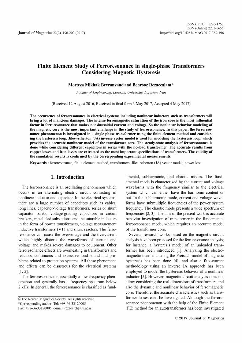
region, as shown in Fig. 3, which leads to a reduction of
simulation time.
One problem regarding the implementation of the JA
model is to determine the corresponding coefficients for
the electromagnetic device under investigation. Determin-
ing the coefficients of JA has been described in [14, 15].
Determining these coefficients for grain-oriented steel is
more complex than the non-oriented one [16]. The
analyzed transformer in this study is made of non-
oriented Fe-Si electrical steel. The coefficients used for
the transformer at no-load condition and without the
capacitor are shown in Table 1.
Figure 4 shows the measured and calculated current
waveforms under no-load condition with input voltage of
60v. It is clearly evident that the non-linear behavior of
the transformer core leads to the non-sinusoidal current.
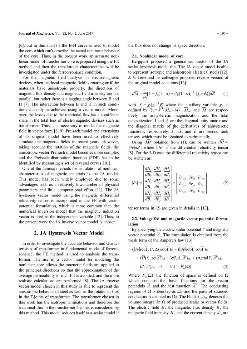
The importance of considering the magnetic hysteresis in
transformer modeling is illustrated in Figs. 4-5 that show
the waveforms and harmonics components of current for
the two cases of modeling using the magnetic hysteresis
and also the anhysteretic B-H curve, it is seen that the
current waveform obtained by employing the magnetic
hysteresis model matches well with the measured current,
in contrast to the one obtained using the anhysteretic B-H
curve.
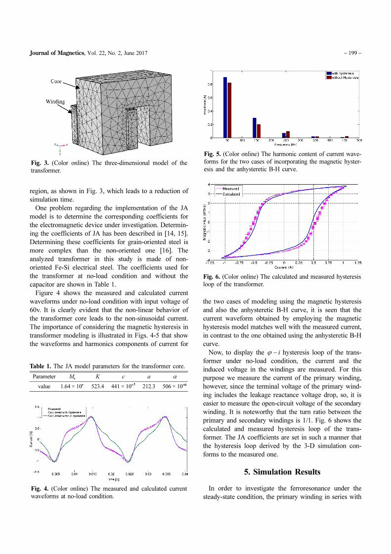
Now, to display the ϕ − i hysteresis loop of the trans-
former under no-load condition, the current and the
induced voltage in the windings are measured. For this
purpose we measure the current of the primary winding,
however, since the terminal voltage of the primary wind-
ing includes the leakage reactance voltage drop, so, it is
easier to measure the open-circuit voltage of the secondary
winding. It is noteworthy that the turn ratio between the
primary and secondary windings is 1/1. Fig. 6 shows the
calculated and measured hysteresis loop of the trans-
former. The JA coefficients are set in such a manner that
the hysteresis loop derived by the 3-D simulation con-
forms to the measured one.
5. Simulation Results
In order to investigate the ferroresonance under the
steady-state condition, the primary winding in series with
Fig. 3. (Color online) The three-dimensional model of the
transformer.
Table 1. The JA model parameters for the transformer core.
Parameter Ms
K c a α
value 1.64 × 10⁶
523.4 441 × 10−3
212.3 506 × 10−6
Fig. 4. (Color online) The measured and calculated current
waveforms at no-load condition.
Fig. 5. (Color online) The harmonic content of current wave-
forms for the two cases of incorporating the magnetic hyster-
esis and the anhysteretic B-H curve.
Fig. 6. (Color online) The calculated and measured hysteresis
loop of the transformer.
− 200 − Finite Element Study of Ferroresonance in single-phase Transformers…
− Morteza Mikhak Beyranvand and Behrooz Rezaeealam
capacitor is fed with 60 V/50 Hz. Then, the capacitance is
varied across the range 10 μF-300 μF in order to study
the transformer specifications in the rated frequency, such
as the voltage and current waveforms and their harmonic
content, the core hysteresis loop, and the core losses. It is
noteworthy that the JA coefficients should be adjusted for
each capacitor value, so that the hysteresis loop imple-
mented in the 3-D simulation matches with the measured
hysteresis loop. Moreover, the residual magnetization is
not included in the modeling.
In the absence of the capacitor, the copper loss and the
core loss of the transformer are 0.14 W, 25.8 W, respec-
tively. These losses severely change with the occurrence
of ferroresonance. By changing the capacitance in series
with the primary winding of the no-load transformer, the
corresponding copper loss and core loss of the transformer
are evaluated in the steady-state, and the results are
shown in Figs. 7 and 8.
Figures 7 and 8 show that the capacitor of 220 μF
causes the intense resonance and imposes the harshest
conditions to the system, and lead to more losses in the
transformer. In this work, the eddy current losses and the
core additional losses are not considered, hence the core
losses achieved through simulation is less than the
measured core loss [17]. As the ferroresonance occurs,
the core loss and copper loss increase dramatically, and it
can be seen that the core losses are much larger than the
copper loss. In the case of prolonged ferroresonance,
thermal damages occur in the transformer and, therefore,
it is necessary to use the grain-oriented steel instead of the
non-oriented one, due to their much narrower hysteresis
loop.
For further inspection of the ferroresonance behavior of
the transformer, the capacitor of 150 μF is connected in
series with the unloaded transformer at time t = 0.2 Sec.
Figure 9 shows that the current increases as ferroreson-
ance occurs and the current waveform at steady-state and
its harmonic content, magnetic hysteresis loop and flux
density distribution are shown in Figs. 10 to 12, respec-
Fig. 7. (Color online) Copper losses versus the capacitance in
series with the transformer.
Fig. 8. (Color online) Core losses versus the capacitance in
series with the transformer.
Fig. 9. (Color online) The current waveform of the Trans-
former (the series capacitor is inserted at t = 0.2 Sec).
Fig. 10. (Color online) The measured and calculated current
waveforms of the unloaded transformer for C = 150 µF. (a)
The current waveform. (b) The FFT of the waveforms.
Journal of Magnetics, Vol. 22, No. 2, June 2017 − 201 −
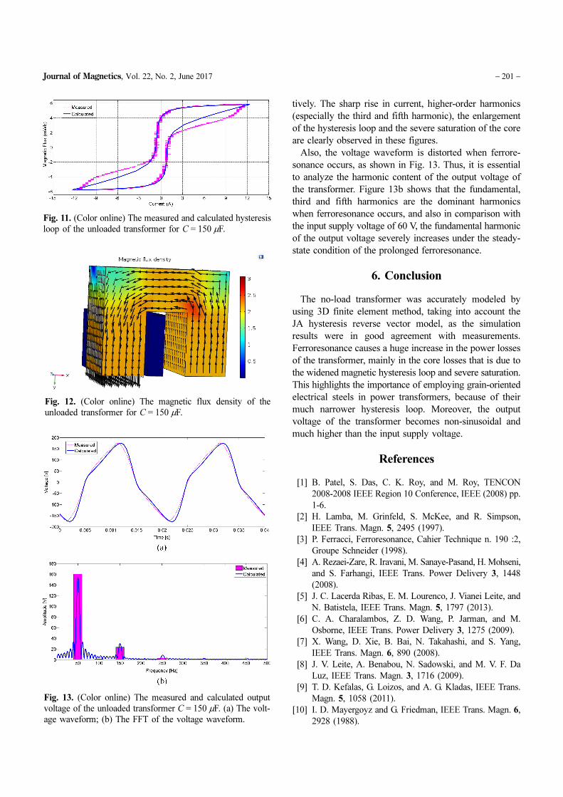
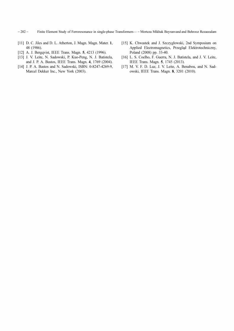
tively. The sharp rise in current, higher-order harmonics
(especially the third and fifth harmonic), the enlargement
of the hysteresis loop and the severe saturation of the core
are clearly observed in these figures.
Also, the voltage waveform is distorted when ferrore-
sonance occurs, as shown in Fig. 13. Thus, it is essential
to analyze the harmonic content of the output voltage of
the transformer. Figure 13b shows that the fundamental,
third and fifth harmonics are the dominant harmonics
when ferroresonance occurs, and also in comparison with
the input supply voltage of 60 V, the fundamental harmonic
of the output voltage severely increases under the steady-
state condition of the prolonged ferroresonance.
6. Conclusion
The no-load transformer was accurately modeled by
using 3D finite element method, taking into account the
JA hysteresis reverse vector model, as the simulation
results were in good agreement with measurements.
Ferroresonance causes a huge increase in the power losses
of the transformer, mainly in the core losses that is due to
the widened magnetic hysteresis loop and severe saturation.
This highlights the importance of employing grain-oriented
electrical steels in power transformers, because of their
much narrower hysteresis loop. Moreover, the output
voltage of the transformer becomes non-sinusoidal and
much higher than the input supply voltage.
References
[1] B. Patel, S. Das, C. K. Roy, and M. Roy, TENCON
2008-2008 IEEE Region 10 Conference, IEEE (2008) pp.
1-6.
[2] H. Lamba, M. Grinfeld, S. McKee, and R. Simpson,
IEEE Trans. Magn. 5, 2495 (1997).
[3] P. Ferracci, Ferroresonance, Cahier Technique n. 190 :2,
Groupe Schneider (1998).
[4] A. Rezaei-Zare, R. Iravani, M. Sanaye-Pasand, H. Mohseni,
and S. Farhangi, IEEE Trans. Power Delivery 3, 1448
(2008).
[5] J. C. Lacerda Ribas, E. M. Lourenco, J. Vianei Leite, and
N. Batistela, IEEE Trans. Magn. 5, 1797 (2013).
[6] C. A. Charalambos, Z. D. Wang, P. Jarman, and M.
Osborne, IEEE Trans. Power Delivery 3, 1275 (2009).
[7] X. Wang, D. Xie, B. Bai, N. Takahashi, and S. Yang,
IEEE Trans. Magn. 6, 890 (2008).
[8] J. V. Leite, A. Benabou, N. Sadowski, and M. V. F. Da
Luz, IEEE Trans. Magn. 3, 1716 (2009).
[9] T. D. Kefalas, G. Loizos, and A. G. Kladas, IEEE Trans.
Magn. 5, 1058 (2011).
[10] I. D. Mayergoyz and G. Friedman, IEEE Trans. Magn. 6,
2928 (1988).
Fig. 11. (Color online) The measured and calculated hysteresis
loop of the unloaded transformer for C = 150 µF.
Fig. 12. (Color online) The magnetic flux density of the
unloaded transformer for C = 150 µF.
Fig. 13. (Color online) The measured and calculated output
voltage of the unloaded transformer C = 150 µF. (a) The volt-
age waveform; (b) The FFT of the voltage waveform.
− 202 − Finite Element Study of Ferroresonance in single-phase Transformers…
− Morteza Mikhak Beyranvand and Behrooz Rezaeealam
[11] D. C. Jiles and D. L. Atherton, J. Magn. Magn. Mater. 1,
48 (1986).
[12] A. J. Bergqvist, IEEE Trans. Magn. 5, 4213 (1996).
[13] J. V. Leite, N. Sadowski, P. Kuo-Peng, N. J. Batistela,
and J. P. A. Bastos, IEEE Trans. Magn. 4, 1769 (2004).
[14] J. P. A. Bastos and N. Sadowski, ISBN: 0-8247-4269-9,
Marcel Dekker Inc., New York (2003).
[15] K. Chwastek and J. Szczygłowski, 2nd Symposium on
Applied Electromagnetics, Przegląd Elektrotechniczny,
Poland (2008) pp. 33-40.
[16] L. S. Coelho, F. Guerra, N. J. Batistela, and J. V. Leite,
IEEE Trans. Magn. 5, 1745 (2013).
[17] M. V. F. D. Luz, J. V. Leite, A. Benabou, and N. Sad-
owski, IEEE Trans. Magn. 8, 3201 (2010).


![Impact of Cattaneo-Christov Heat Flux Model on the Flow of …komag.org/journal/download.html?file_name=5826bec375360a... · Cattaneo [5] remodel the Fourier law by including thermal](https://static.documents.pub/doc/80x56/60c797d9bccc441e4109ac2f/impact-of-cattaneo-christov-heat-flux-model-on-the-flow-of-komagorgjournal-filename5826bec375360a.jpg)


![Effects of Magnetized Medium on In Vitro Maturation of ...komag.org/journal/download.html?file_name=1411610636.pdf · block during early cleavage stage and mitotic arrest [8-10].](https://static.documents.pub/doc/80x56/5fe61a3b08848f26d22edf0b/effects-of-magnetized-medium-on-in-vitro-maturation-of-komagorgjournal-filename1411610636pdf.jpg)

![A Study on the Effective Deperming Protocol Considering …komag.org/journal/download.html?file_name=e4c90f35641d07... · deperming protocol [1-3]. Three types of deperming protocols](https://static.documents.pub/doc/80x56/60ca848d0857e82d3b607729/a-study-on-the-effective-deperming-protocol-considering-komagorgjournal-filenamee4c90f35641d07.jpg)


