Firm productivity and export markets: a non … · Firm productivity and export markets: a...

Journal of International Economics 57 (2002) 397–422www.elsevier.com/ locate /econbase

Firm productivity and export markets: a non-parametricapproach

a , b c* ˜Miguel A. Delgado , Jose C. Farinas , Sonia Ruanoa Úniversidad Carlos III de Madrid, Departomento de Econometrıa, C. /Madrid 126-128,

28903 Getafe, Madrid, Spainb Úniversidad Complutense de Madrid; Facultad de Ciencias Economicas,

´Departomento de Economıa Aplicada II, Madrid 28223, Spainc ˜Universidad Carlos III de Madrid and Banco de Espana, C. /Madrid 126-128, Getafe,

Madrid 28903, Spain

Received 18 January 2000; received in revised form 30 January 2001; accepted 25 June 2001

Abstract

This paper examines total factor productivity differences between exporting and non-exporting firms. These differences are documented on the basis of a sample of Spanishmanufacturing firms over the period 1991–1996. The paper also examines two complemen-tary explanations for the greater productivity of exporting firms: (1) the market selectionhypothesis, and (2) the learning hypothesis. Non-parametric tests are proposed andimplemented for testing these hypotheses. Results indicate clearly higher levels ofproductivity for exporting firms than for non-exporting firms. With respect to the relativemerits of the selection and the learning hypotheses, we find evidence supporting theself-selection of more productive firms in the export market. The evidence in favor oflearning-by-exporting is rather weak, and limited to younger exporters. 2002 ElsevierScience B.V. All rights reserved.

Keywords: Total factor productivity; Exports; Stochastic dominance; Non-parametric tests

JEL classification: D24; F10; M20; L10

*Corresponding author. Tel.: 1 34-916-24-9804; fax: 1 34-916-24-9849.E-mail address: [email protected] (M.A. Delgado).

0022-1996/02/$ – see front matter 2002 Elsevier Science B.V. All rights reserved.PI I : S0022-1996( 01 )00154-4

398 M.A. Delgado et al. / Journal of International Economics 57 (2002) 397 –422

1. Introduction

The link between efficiency and exports is one of the many features which theliterature concerning productivity growth has focused on. A widespread and robustfinding supported by this literature is the existence of significant differences inproductivity among firms. Furthermore, it has also been observed that thesedifferences persist (see Griliches and Regev, 1995, and many others; for a reviewarticle see Tybout, 1997). One of the firms’ characteristics that contributes to thisobserved heterogeneity is the entry of firms into the export market. Studies by Awand Hwang (1995), Bernard and Jensen (1995), Jensen and Wagner (1997), Aw etal. (1997), Clerides et al. (1998) and Aw et al. (2000), provide evidence on thefact that export-oriented firms are closer to the efficiency frontier than non-exporters.

The purpose of this paper is to measure total factor productivity differencesbetween exporting and non-exporting firms. First, the paper documents theseproductivity differences on the basis of a panel sample of Spanish manufacturingfirms over the period 1991–1996. Therefore, we contribute to the growing body ofempirical literature that examines the relationship between productivity andexports, adding another national perspective to the available evidence. Theproposed methodological approach is the second contribution of the paper. Wecompare the entire distribution of productivities rather than just marginal mo-ments. In particular, we compare the cumulative distribution functions of totalfactor productivity for different groups of firms: exporters, non-exporters, enteringexporters and exiting exporters. These distributions are ranked using the conceptof stochastic dominance, and their differences are formally tested using Kol-mogorov–Smirnov one and two-sided tests, which are consistent in the directionof general non-parametric alternatives. Third, the paper makes an attempt atsorting out the selection versus the learning explanations for the superiorproductivity of exporting firms. The paper explores and tests for these twodifferent, but non-mutually exclusive explanations by comparing productivitylevels as well as productivity growth for groups of firms with different trajectoriesbetween the export and domestic markets.

Our empirical findings confirm higher levels of productivity for exporting firmsversus non-exporting firms. With respect to the relative merits of the selection andthe learning hypotheses proposed to explain the greater productivity of exporters,we find evidence supporting the self-selection of more productive firms into theexport market. The evidence in favor of the learning-by-exporting hypothesis israther weak, and limited to younger exporters. These results are very much in linewith those reported by Clerides et al. (1998), Bernard and Jensen (1999), and Awet al. (2000). Although the methodology used differs throughout their research,they all come to a similar conclusion: market selection rather than learning-by-exporting is the factor that leads to higher productivity of exporting firms withrespect to non-exporting firms.

M.A. Delgado et al. / Journal of International Economics 57 (2002) 397 –422 399

The rest of the paper is organized as follows. Section 2 summarizes theanalytical arguments for the observed link between productivity and exports, andpresents the testing procedures that have been used throughout the paper. Section 3describes the data set, the index used for measuring total factor productivity andsome general estimation issues. Section 4 reports the main empirical results.Conclusions are placed in Section 5.

2. Analytical framework

2.1. Productivity differentials and exports

To explain why exporters are more efficient than non-exporters, the analyticalliterature on productivity has outlined two arguments: (1) firms participating ininternational markets are exposed to more intensive competition; and (2) exportershave higher sunk entry costs than domestic firms. Both explanations share the ideathat export markets select the most efficient firms among the set of potentialentrants into the export market. The first argument is present in the literatureconcerning development economics and relies on the idea that product marketcompetition in export markets is greater than competition in domestic markets and,therefore, affords fewer opportunities for inefficient firms (see Aw and Hwang,1995, for further details on these arguments.) Empirical studies on trade reform(see Feenstra, 1997, for a survey) confirm the existence of a positive relationshipbetween competition and productivity.

The second argument to the explanation of superior productivity of exportingfirms comes from models of industry dynamics by Jovanovic (1982), Hopenhayn(1992) and Ericson and Pakes (1995). These models predict the existence of asystematic relationship between patterns of entry and exit and productivitydifferences at the firm level. As Aw et al. (1997) argue, a similar statement appliesto the relationship between export markets and productivity. Even if we considerthat the competitive pressure in the domestic market and the export market issimilar, differences in sunk entry costs can explain productivity differencesbetween exporters and domestic-oriented firms. The basic assumption underlyingthis argument is that a non-exporter must incur a sunk entry cost in order to enterthe export market. Recent studies confirm this assumption empirically: Robertsand Tybout (1997) find that firm’s previous export status is an importantdeterminant of the decision to export and they interpret this as a favorableevidence to the existence of sunk entry costs in the export market. In particular,Campa (1998) finds that exporting sunk entry costs are important for Spanishmanufacturing firms.

Models of industry dynamics have two consequences for the analysis ofproductivity differences between exporting and non-exporting firms. First, higherentry costs for firms entering the export market with respect to those firms selling


in the domestic market imply higher productivity levels for exporting firms.Second, patterns of entry and exit in the export market are related to productivitydifferences at the firm level. On one hand, the productivity distribution ofcontinuing exporters should stochastically dominate the distribution of enteringand exiting exporters. On the other hand, entering exporters should have higherinitial productivity relative to firms that remain outside of the export market.

The two outlined arguments are consistent with the hypothesis of selection. Athird argument, not mutually exclusive with respect to the two previous ones, isbased on the idea of exporting as a learning mechanism that allows firms toimprove their productivity. The management literature describing the inter-nationalization process either as a sequence of stages for the firm or as aninnovation for the firm, has emphasized the notion of exporting as a learningprocess.

To organize our empirical work we rely on the previous arguments, whichsuggest the following hypotheses be tested based on the concept of stochasticdominance:

(i) If productivity differences reflect selection and/or learning forces at work inexport markets, the productivity distribution of exporting firms should dominatethe productivity distribution of non-exporting firms.

(ii) Self-selection implies that differences between exporting and non-exportingfirms precede their entry in the export market. Therefore, in the period prior totheir entry, the productivity distribution of entering exporters should dominate theproductivity distribution of non-exporters.

(iii) Selection on the exit side of the market implies that the productivitydistribution of continuing exporters should dominate the distribution of exitingexporters.

(iv) Finally, if the empirical consequences of learning-by-exporting are consid-ered as well, differences between productivity levels for exporting and non-exporting firms should increase after the entry of exporters in the export market.Therefore, the productivity growth distribution of entering exporters shoulddominate the distribution of non-exporting firms.

In the next section we describe a testing procedure for examining productivitydifferentials between groups of firms with different trajectories between thedomestic and the export market.

2.2. Testing procedure

This section develops a procedure for comparing the productivity distributionsof different groups of firms. The panel structure of the sample of firms allows aclassification of firms according to their trajectories between the export and thedomestic market over a given period. We have designed different tests to explorewhether or not transitions from domestic to export markets are consistent withfirms’ productivity differences summarized in Section 2.1.


Most of the empirical questions we are interested in can be formulated ascomparisons between the distributions of firm productivity level or firm prod-uctivity growth corresponding to different groups in the population. Our procedurefor testing differences between distribution functions relies on the concept of firstorder stochastic dominance and permits us to establish a ranking for the compareddistributions. Let F and G denote the cumulative distribution functions ofproductivity corresponding to two groups of firms that have to be compared, then(first order) stochastic dominance of F relative to G is defined by the followingcondition: F(z) 2 G(z) # 0 uniformly in z [ R, with strict inequality for some z.

Let Z , . . . ,Z , be a random sample of size n, which corresponds to a group of1 n

firms, from the distribution function F, and let Z , . . . ,Z , denote a randomn11 n1m

sample of size m, independent of the first one, which corresponds to a differentgroup of firms, from the distribution function G; where Z represents either thei

productivity level or the productivity growth of firm i. We are interested in testingthe following hypotheses:

(i) Two sided test

H : F(z) 2 G(z) 5 0 all z [ R vs. H : F(z) 2 G(z) ± 0 some z [ R0 1

can be rejected.(ii) One-sided test

H : F(z) 2 G(z) # 0 all z [ R vs. H : F(z) 2 G(z) . 0 some z [ R0 1

cannot be rejected.One and two-sided test can also be formulated as

H : sup F(z) 2 G(z) 5 0 vs. H : sup F(z) 2 G(z) ± 0u u u u0 1z[R z[R

and

H : sup F(z) 2 G(z) 5 0 vs. H : sup F(z) 2 G(z) . 0 ,h j h j0 1z[R z[R

respectively. To give a more intuitive explanation let us suppose that F and Grepresent the productivity distributions for exporters and non-exporters, respective-ly. On one hand, the two-sided test allows us to determine whether bothdistributions are identical or not. On the other hand, the one-sided test permits usto determine whether or not a distribution dominates the other. Particularly, whenthe two-sided test is rejected and the one-sided test cannot be rejected, it indicatesthat F is to the right of G. In other words, it implies that exporters’ productivitydistribution stochastically dominates non-exporters’ productivity distribution.

The Kolmogorov–Smirnov test statistics for these one and two-sided tests are

]n.m]d 5 max T (Z )u uN N iœ N 1#i#N

and


]n.m]h 5 max T (Z ) ,h jN N iœ N 1#i#N

respectively, where T (Z ) 5 F (Z ) 2 G (Z ) and N 5 n 1 m. F and G representN i n i m i n m

the empirical distribution functions for F and G, respectively. The limiting1distributions of both test statistics, d and h , are known under independence .N N

3. Measurement and estimation issues

3.1. The data

The data set considered in this study is drawn from the ‘Encuesta sobreEstrategias Empresariales’ (ESEE), an annual survey which refers to a representa-tive sample of Spanish manufacturing firms. A first characteristic of the data set isthat, in the base year, firms were chosen according to a selective sampling schemewith different probabilities of firm participation depending on their size category.All firms with more than 200 employees (large firms) were asked to participate,and the rate of participation reached approximately 70% of the population of firmswithin that size category. Firms that employed between 10 and 200 employees(small firms) were chosen according to a random sampling scheme, and the rate ofparticipation was close to 5% of the number of firms in the population. The sameselection scheme was applied to every industry. Therefore, the coverage of thedata set is different depending on the size group of firms. Consequently, given theprocedure used to incorporate firms into the survey, the characteristics of thedistribution of Spanish manufacturing firms, for given size groups and industries,can be estimated from our sample.

A second characteristic of the data set is that in subsequent years the initialsample properties have been maintained. On one hand, newly created firms havebeen added annually with the same sampling criteria as in the base year (seeMinistry of Industry, 1992, for technical details.) On the other hand, exiting firmshave been recorded in the sample of firms surveyed each year. Therefore, due tothis entry and exit process, the data set is an unbalanced panel of firms.

Over the period 1991–1996, the data set has collected 10,595 observations atthe firm level that correspond to an average number of 1766 firms throughout theentire period. The yearly average distribution of firms can be classified, fordescriptive purposes, into five groups according to their export participation alongthe time period: exporters, non-exporters, entering exporters, exiting exporters and

1These test statistics were proposed by Smirnov (1939). Kolmogorov (1933) and Smirnov (1939)showed that, under the assumption that all the observations are independent, the limiting distributions

` k 2 2of d and h under H are given by lim P(d . y) 5 2 2o (21) exp(22k y ) and limN N 0 N k51N→` N→`2P(h . y) 5 exp(22y ), respectively. For more details see Darling (1957).N


switchers. For the first two groups – firms that export every year and firms that donot export along the time period – figures indicate that there is a positiverelationship between the size of firms and their participation in the export market:78% of large firms export regularly while the rate of participation for small firmsis 27%. Firm turnover with respect to the export market corresponds to the groupof entering exporters – firms becoming exporters during the period without furtherchanges in the rest of the period – and to the group of exiting exporters – firmsceasing to export and not reswitching. Two features should be noted. First, thefraction of firms entering and exiting the export market implies a high turnoverrate. The annual average rate for small firms is 16 and 11% for large firms.Second, during the period the average entry rate is higher than the average exitrate. This difference suggests that the large increase in Spanish exports during thenineties has been partly due to a net increase in the number of exporting firms.Finally, the group of switchers – firms that change their export status more thanonce during the period – represents 11 and 6% for small and large firms,respectively.

3.2. The measurement of firm productivity

This section presents an index for measuring firm productivity that follows theframework developed in Aw et al. (2000). The index is an extension of themultilateral total factor productivity index proposed by Caves et al. (1982) thatuses the average firm of the firm’s size group as a reference point and thenchain-links the reference points to preserve transitiveness. This extension takesinto account the characteristics of the data set, in particular, the fact that samplingproportions are different for small and large firms. A similar extension of the indexcan be found in Good et al. (1996). The main advantage of this kind of measure isthat the parameters of the production function are not required to computeproductivity.

The ESEE provides observations

k kY , W , X , k 5 1, . . . ,K , f 5 1, . . . ,N, t 5 1, . . . ,T ,hs d jft ft ft

k kwhere Y is the output level of the firm f at time t, W and X are, respectively, theft ft ft

cost share and the quantity of input k corresponding to firm f at time t. Thedefinition of the three inputs considered (labor, materials and capital) and outputcan be found in Appendix A. Capital letters denote the number of firms (N), thenumber of time periods (T ) and the number of inputs (K). Firms are classified in

2two size groups and I different industries . Let us introduce the dummy variables,

2Firms have been grouped in 18 industries corresponding to NACE-CLIO R-25 classification.


s 5 1 firm f belongs to size group ts dft

i 5 1 firm f belongs to industry r ,s dfr

where 1 A is the indicator function of event A. It is assumed that observations fors ddifferent firms, at a given period, are independent. It is also assumed that thedistributions of the variables at different periods can be different, so we do notassume stationarity. The expression of total factor productivity index at time t, forthe firm f, which belongs to the size group t and to the industry r is

K1] ] ]k k k k]ln l 5 ln Y 2ln Y 2 O W 1W ln X 2ln Xs ds dft ft tr ft tr ft tr2 k51K1] ] ] ] ] ]k k k k]1ln Y 2ln Y 2 O W 1W ln X 2ln X ,s ds dtr r tr r tr r2 k51

where, for notational convenience, we drop reference to the size group, t, andk kindustry, r; and for a generic variable a , which can be ln Y , W or ln Xft ft ft ft

N T N T1 1] ]] ]a 5 O O a s i and a 5 O Oa i .tr ft ft fr r ft frNT NTt51 t51f51 f51

This index measures the proportional difference of total factor productivity forfirm f at time t relative to a given reference firm. The reference firm varies acrossindustries and, for a given industry r, it is defined as the firm such that: (i) itsoutput is equal to the geometric mean of firms output quantities in industry r overthe entire period; (ii) the quantities of inputs are equal to the geometric means offirms input quantities in industry r over the entire period; and (iii) the cost sharesof inputs are equal to the arithmetic mean of firms cost shares in industry r overthe entire period. Notice that the reference firm varies across industries and,therefore, when observations of different industries are pooled, productivitydifferences among industries are removed.

To clarify the meaning of the productivity index, we can interpret the terms onthe right hand side separately. The first set of terms compares the firm with theaverage firm of the same size group, which is taken as reference. Hence,comparisons between observations corresponding to the same size group aretransitive. The second set of terms measures productivity differences between thereference firm of a size group and a common reference firm, which is the averagefirm over the entire sample of firms in industry r. Thus, comparisons betweenobservations corresponding to different size groups are also transitive. Consider,for example that firm f belongs to industry r and employs more than 200 workers.The first set of terms gives the proportional difference of total factor productivityfor firm f at time t with respect to the average firm in the group of large firmsproducing in industry r. The second set of terms, adds the proportional difference


between the reference firm for the group of large firms in industry r and thecommon reference firm for both size groups in this industry.

3.3. Implementation of the tests

In this section we discuss some issues related to the application of one andtwo-sided Kolmogorov–Smirnov tests to our data set. In particular, there are fourquestions that have to be considered.

First, the application of the testing procedure defined in Section 2.2 requiresindependence of the observations. Given the panel structure of our sample offirms, observations for different years correspond to firms that are repeated, andtherefore cannot be considered either independent or stationary. Consequently, theapplication of Kolmogorov–Smirnov tests has to be done separately for each timeperiod.

Second, testing for stochastic dominance requires the use of empirical dis-tributions of the compared groups of firms. Given the sampling properties of ourdata set, we use cumulative distribution functions for the two size categories (smalland large firms,). Comparisons between distribution functions for the wholepopulation are avoided since this would have required the estimation of a mixtureof two distributions. Therefore, we compare different groups of firms, i.e.exporters and non-exporters, within the same size category or between size-categories (the productivity index preserves transitiveness along the two sizecategories).

Third, it should be notice that our productivity measure, ln l , can beft

*interpreted as an estimate of a non-observable measure, say ln l , with sampleft

averages replaced by population means. The Kolmogorov–Smirnov’s test is*directly applicable to ln l . However, the limiting process of the sampleft

distribution of ln l , which contains estimated parameters, depends on certainft

unknown features of the data generating process, and the empirical distributionfunction converges to a non-pivotal process (see e.g. Durbin, 1973). Bai (1996)has shown that structural stability tests, which are a type of two-sample test, fordistribution functions based on residuals of linear regression models are dis-tribution free. Also, Delgado and Mora (2000) have shown that independence testsbased on the difference between the joint distribution and the product of marginaldistributions (Hoeffding–Blum–Kiefer–Rosenblatt test) are also distribution freewhen residuals, rather than observations, are employed. Despite the fact that thisresult has not been extended to two-sample problems for general functionsdepending non-linearly on estimated parameters, in a earlier version of this paper(see Delgado et al., 1999) we have proved formally that asymptotic Kolmogorov–Smirnov’s tests is also distribution free. Therefore, we can use the same tables for

*the test based on ln l and the infeasible ln l .ft ft

Fourth, we provide two P-values for each of the statistics: one based on thelimiting distribution and the other on the bootstrap approximation. Asymptotic and


bootstrap P-values are fairly close, which illustrates the good accuracy of theasymptotic approximation. The ‘naive’ bootstrap for empirical processes has been

´justified by Gine and Zinn (1990). Bootstrap P-values are computed in our contextas follows.

* * * * *(a) Obtain a resample x 5 z , . . . ,z , z , . . . ,z by random samplingh jN 1 n n11 n1m

with replacement from x 5 z , . . . ,z , z , . . . ,z .h jN 1 n n11 n1m

* *(b) Compute bootstrap analogs of d and h , say d and h , based on theN N N N

*resample x .N

The bootstrap P-values are

*P*-value(d ) 5 Pr d $ d uxh jN N N N

*P*-value(h ) 5 Pr h $h ux .h jN N N N

Calculating these P-values is computationally unapproachable in practice.However, they can be approximated, as accurately as desired, by Monte Carlo.That is, we repeat steps (a) and (b) B times, B as large as desired accuracy,

b b* *obtaining bootstrap statistics d and h , b 5 1, . . . ,B. The bootstrap P-valuesN N

are approximated by

B1 b]* *P -value(d ) 5 O 1(d $ d )B N N NB b51B1 b]* *P -value(h ) 5 O 1(h $h ).B N N NB b51

Under H , the bootstrap P-values converge to zero almost surely.1

To further illustrate the comparisons between different groups of firms we havegraphed estimates of the distribution functions. In particular, we have computedthe smooth, or perturbed, sample distribution function, rather than the sampledistribution function itself, which provides nice smooth distribution estimates. Thesmooth sample distribution estimator was proposed by Nadaraya (1964). Since thepurpose here is to produce graphical representations of the differences betweentwo groups of firms, we represent these distributions for the whole population offirms. Consider for that purpose the distribution F (.), which corresponds to thet

productivity of, say, exporting firms, and F (.ut 5 t ), t 5 0,1 , which denotes theh jt 0 0

conditional distribution function for a given size group of firms – small (t 5 0) orlarge (t 5 1). The selective sampling scheme used in our data set implies that onlythese conditional cumulative distribution functions, F (.ut 5 t ), can be estimatedt 0

directly. However, the cumulative distribution function for the whole population ofexporters can be obtained by the following expression:

F (.) 5 P (t 5 0) 3 F (.ut 5 0) 1 P (t 5 1) 3 F (.ut 5 1) (1)t t t t t

where P (.) represents the probability of being either a small or a large firm in thet

considered group of exporting firms. This expression indicates that the cumulative


distribution function for the whole population of firms can be estimated as aweighted average of the two conditional cumulative distribution functions.Marginal probabilities can be calculated from the information provided by the

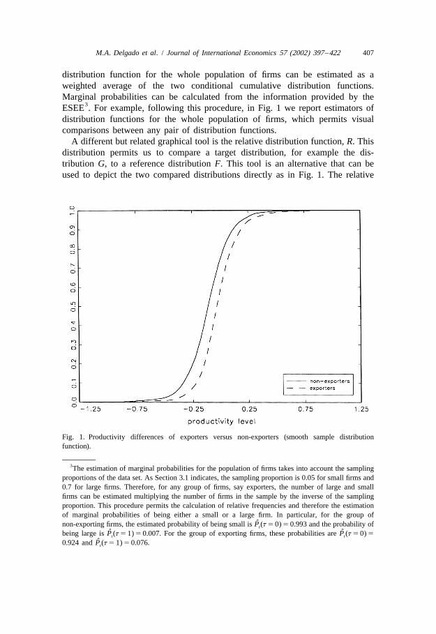
3ESEE . For example, following this procedure, in Fig. 1 we report estimators ofdistribution functions for the whole population of firms, which permits visualcomparisons between any pair of distribution functions.

A different but related graphical tool is the relative distribution function, R. Thisdistribution permits us to compare a target distribution, for example the dis-tribution G, to a reference distribution F. This tool is an alternative that can beused to depict the two compared distributions directly as in Fig. 1. The relative

Fig. 1. Productivity differences of exporters versus non-exporters (smooth sample distributionfunction).

3The estimation of marginal probabilities for the population of firms takes into account the samplingproportions of the data set. As Section 3.1 indicates, the sampling proportion is 0.05 for small firms and0.7 for large firms. Therefore, for any group of firms, say exporters, the number of large and smallfirms can be estimated multiplying the number of firms in the sample by the inverse of the samplingproportion. This procedure permits the calculation of relative frequencies and therefore the estimationof marginal probabilities of being either a small or a large firm. In particular, for the group of

ˆnon-exporting firms, the estimated probability of being small is P (t 5 0) 5 0.993 and the probability oft

ˆ ˆbeing large is P (t 5 1) 5 0.007. For the group of exporting firms, these probabilities are P (t 5 0) 5t t

ˆ0.924 and P (t 5 1) 5 0.076.t


Fig. 2. Relative distribution functions of exporters’ productivity to non-exporters’ productivity:1991–96.

21distribution is defined as R r 5 GsF r d, where 0 # r # 1. Notice that if boths d s d21distributions are identical, then the relative distribution, i.e. FsF r d, is thes d

uniform distribution on [0,1]. Fig. 2 provides an example of the comparisonbetween two distributions over several years. The diagonal represents the uniformdistribution, i.e. the relative distribution if both distributions were identical. Theposition of the relative distribution below the diagonal suggests that the dis-tribution represented in the vertical axis stochastically dominates the distribution inthe horizontal axis.

The next section presents the results based on formal tests of the differencesbetween various groups of firms. Systematic visual representations of thecompared distributions are also included.

4. Empirical results

This section is organized as follows. First, we begin by examining differences intotal factor productivity between exporters and non-exporters. Second, we explorea possible source for the observed differences between exporting and non-exporting firms by examining if firm transitions between the domestic and theexport market are consistent with certain patterns of productivity differences. We


make two comparisons: (1) ex-ante productivity differentials between firmsentering into the export market and non-exporters and (2) productivity differencesbetween exiting exporters and continuing exporters. Finally, we examine whetheror not productivity growth of firms in contact with the export market is greaterthan the productivity growth of non-exporters. All these comparisons are carriedout through non-parametric methods described in previous sections.

4.1. Exports and productivity

We begin the analysis of the relationship between productivity and exports byexamining the magnitude of productivity differentials between exporting firms andnon-exporting firms. Exporters are defined as firms that export at period t, andnon-exporters are firms not selling abroad at t; in both cases switchers areexcluded. Very frequently, switchers are a special type of exporting firm that sellsabroad intermittently, in time intervals greater than a year. For this reason, thegroup of firms switching their export status more than once during the givenperiod are excluded from the comparison. However, results reported below do notchange when switchers are included in accordance to their export status in year t.

Fig. 1 illustrates the differences between the productivity distributions ofexporting and non-exporting firms in year 1996 within the whole population offirms. The position of the distribution for exporting firms with respect to thedistribution of non-exporting firms indicates higher levels of productivity forexporters versus non-exporters. All quartiles of the productivity distributions arehigher for exporting firms relative to non-exporting firms. In particular, the medianproductivity of the former is 7% higher than the productivity of the latter.Productivity differences are greater at the lower part of the distribution, 10% infavor of exporting firms at the lower quartile, and smaller in the upper part, 5% infavor of exporting firms at the upper quartile.

Fig. 2 shows the relative distribution of exporting firms with respect tonon-exporting firms for all of the years in the period 1991–1996. The relativedistribution is a graphical tool for the comparison of two distributions. As Fig. 2illustrates, the position of the relative distribution of exporters to non-exporters isbelow the diagonal during the whole period; suggesting that the productivitydistribution of exporters stochastically dominates the distribution of non-exporters.In 1996 around 50% of non-exporting firms’ productivity is below the 30%quartile of exporting firms’ productivity.

Given the assessed differences, now we formally test to see if the productivitydistribution of exporting firms stochastically dominates the productivity dis-tribution of non-exporting firms For each time period and size group t , we0

compare

F (.ut 5 t ) vs. G (.ut 5 t ), t 5 1991, . . . ,1996 and t 5 0,1t 0 t 0 0

using the one and two-sided tests described in Section 2.2, where F and G denotet t

410M

.A.

Delgado

etal.

/Journal

ofInternational

Econom

ics57

(2002)397

–422

Table 1Productivity level differences between exporters and non-exporters; hypotheses test statistics

Year Small exporting firms vs. small non-exporting firms Large exporting firms vs. large non-exporting firms

Number of observations Equality of Differences favorable Number of observations Equality of Differences favorable

Exporters Non- distributions to exporters Exporters Non- distributions to exporters

a a a aexporters Statistic P-value Statistic P-value exporters Statistic P-value Statistic P-value

1991 361 725 2.270 0.000 0.384 0.745 598 82 0.956 0.320 0.272 0.862

(0.000) (0.729) (0.304) (0.835)

1992 373 730 2.152 0.000 0.088 0.985 541 63 0.872 0.432 0.872 0.218

(0.000) (0.975) (0.373) (0.180)

1993 395 673 2.604 0.000 0.016 0.999 457 47 0.512 0.956 0.433 0.687

(0.000) (0.998) (0.926) (0.606)

1994 428 606 3.544 0.000 0.000 1.000 510 48 0.750 0.627 0.357 0.775

(0.000) (1.000) (0.577) (0.739)

1995 441 519 3.529 0.000 0.000 1.000 470 43 0.825 0.505 0.450 0.667

(0.000) (1.000) (0.454) (0.649)

1996 477 537 3.771 0.000 0.030 0.998 447 37 0.615 0.843 0.454 0.662

(0.000) (0.997) (0.777) (0.618)

a P-values are based on the limiting distribution. P-values based on the bootstrap approximation (10 000 replications) are presented in parenthesis.


the productivity level (ln l ) distribution for exporting firms and non-exportingft

firms in year t, respectively.Table 1 presents the hypotheses test statistics of productivity differentials

between exporters and non-exporters. Tests are applied separately both to thegroups of small and large firms. First, for the group of small firms, the nullhypothesis of equality between both distributions can be rejected at the 0.01 levelfor all years. The null hypothesis that the sign of the difference is as expected, i.e.small exporters have greater productivity than small non-exporters, cannot berejected at any reasonable significance level. Second, for the groups of largeexporters and non-exporters, the equality of both productivity distributions cannotbe rejected at any reasonable significance level. Although productivity differencesbetween exporters and non-exporters are rather modest in the group of large firms,they favor large exporters with respect to non-exporters, as suggested by teststatistics reported in Table 1. P-values based both on the limiting distribution andon the bootstrap approximation lead to the same results.

Two conclusions can be derived from previous test statistics: (1) the productivi-ty distribution of small exporting firms stochastically dominates the productivitydistribution of small non-exporting firms; and (2) the productivity distribution oflarge exporting firms is not above the productivity distribution of large non-exporting firms. To obtain conclusions about productivity differences in the wholepopulation of firms, some additional comparison across size groups is required. Inparticular, the difference between exporters and non-exporters, [F (.) 2 G (.)], cant t

be expressed as a linear combination of productivity differences in the group ofsmall firms [F (.ut 5 0) 2 G (.ut 5 0)], the group of large firms [F (.ut 5 1) 2t t t

G (.ut 5 1)], and differences between large non-exporting firms and small non-t

exporting firms [G (.ut 5 1) 2 G (.ut 5 0)]. A formal test of this latter differencet t

leads to the conclusion that the productivity distribution of large non-exportingfirms stochastically dominates the distribution of small non-exporting firms.Furthermore, the parameters weighting the linear combination are positive.Therefore, our results can also be interpreted as evidence supporting the hypoth-esis that in the whole population of firms, exporters stochastically dominatenon-exporters.

4.2. Productivity and transitions between the domestic and the export market

We turn now to the consideration of possible sources for productivity differ-ences between exporting and non-exporting firms. We explore whether or not thehigher productivity of exporters reflects selection forces at work, i.e. exportmarkets selecting the most efficient firms. This selection mechanism can workboth on the entry side and on the exit side. On the entry side, the implication ofselection is that only firms with higher productivity should enter the export market.On the exit side, if selection is at work, low productivity exporters should leavethe export market.


To test for selection on the entry side of the export market, we compare twogroups of firms: non-exporters and entering exporters. To define both groups wetake as a reference the set of non-exporting firms in 1991. Entering exporters aredefined as the group of firms entering the export market at some point between1992 and 1996. The rest of firms defines the group of non-exporters. Switchers areexcluded from the comparison. We consider a 5 year entry period that permits us toenlarge the number of observations. The test performed compares the productivitylevel of both groups of firms in the year 1991, before entry took place for thegroup of entering exporters.

For the whole population of firms, Fig. 3 reports kernel estimators of thecumulative distribution functions of productivity for non-exporters and enteringexporters. Both distributions correspond to the year 1991. The distribution positionfor entering firms is to the right of the position of non-exporters, indicating thatfirms that eventually enter the export market were more efficient than non-exporters. To examine this difference more formally, we test to see if theproductivity level distribution of entering firms in the export market stochasticallydominates the productivity distribution of non-exporters during the period beforeentry took place. Consequently, we apply the one and two-sided tests to compare

F (.ut 5 t ) vs. G (.ut 5 t ), t 5 1991 and t 5 0,1,t 0 t 0 0

Fig. 3. Ex-ante productivity differences of entering exporters versus non-exporters: 1992–1996 cohortof entering firms (smooth sample distribution function).


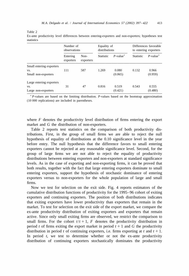
Table 2Ex-ante productivity level differences between entering-exporters and non-exporters; hypotheses teststatistics

Number of Equality of Differences favorableobservations distributions to entering exporters

a aEntering Non- Statistic P-value Statistic P-valueexporters exporters

Small entering exportersvs. 111 587 1.269 0.080 0.132 0.966Small non-exporters (0.065) (0.959)

Large entering exportersvs. 31 47 0.816 0.519 0.543 0.555Large non-exporters (0.421) (0.480)

a P-values are based on the limiting distribution. P-values based on the bootstrap approximation(10 000 replications) are included in parentheses.

where F denotes the productivity level distribution of firms entering the exportmarket and G the distribution of non-exporters.

Table 2 reports test statistics on the comparison of both productivity dis-tributions. First, in the group of small firms we are able to reject the nullhypothesis of equality of distributions at the 0.10 significance level in the yearbefore entry. The null hypothesis that the difference favors to small enteringexporters cannot be rejected at any reasonable significance level. Second, for thegroup of large firms we are not able to reject the equality of productivitydistributions between entering exporters and non-exporters at standard significancelevels. As in the case of exporting and non-exporting firms, it can be proved thatboth results, together with the fact that large entering exporters dominate to smallentering exporters, support the hypothesis of stochastic dominance of enteringexporters versus to non-exporters for the whole population of large and smallfirms.

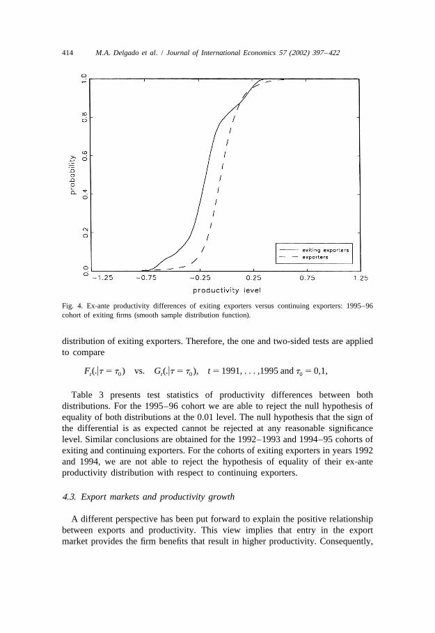
Now we test for selection on the exit side. Fig. 4 reports estimators of thecumulative distribution functions of productivity for the 1995–96 cohort of exitingexporters and continuing exporters. The position of both distributions indicatesthat exiting exporters have lower productivity than exporters that remain in themarket. To test for selection on the exit side of the export market, we compare theex-ante productivity distribution of exiting exporters and exporters that remainactive. Since only small exiting firms are observed, we restrict the comparison tosmall firms. For the cohort t /t 1 1, F denotes the productivity distribution inperiod t of firms exiting the export market in period t 1 1 and G the productivitydistribution in period t of continuing exporters, i.e. firms exporting at t and t 1 1.In period t, we test to determine whether or not the ex-ante productivitydistribution of continuing exporters stochastically dominates the productivity


Fig. 4. Ex-ante productivity differences of exiting exporters versus continuing exporters: 1995–96cohort of exiting firms (smooth sample distribution function).

distribution of exiting exporters. Therefore, the one and two-sided tests are appliedto compare

F (.ut 5 t ) vs. G (.ut 5 t ), t 5 1991, . . . ,1995 and t 5 0,1,t 0 t 0 0

Table 3 presents test statistics of productivity differences between bothdistributions. For the 1995–96 cohort we are able to reject the null hypothesis ofequality of both distributions at the 0.01 level. The null hypothesis that the sign ofthe differential is as expected cannot be rejected at any reasonable significancelevel. Similar conclusions are obtained for the 1992–1993 and 1994–95 cohorts ofexiting and continuing exporters. For the cohorts of exiting exporters in years 1992and 1994, we are not able to reject the hypothesis of equality of their ex-anteproductivity distribution with respect to continuing exporters.

4.3. Export markets and productivity growth

A different perspective has been put forward to explain the positive relationshipbetween exports and productivity. This view implies that entry in the exportmarket provides the firm benefits that result in higher productivity. Consequently,


Table 3Ex-ante productivity level differences between exiting exporters and continuing exporters; hypothesestest statistics

Year Small exiting exporters vs. small continuing exporters

Number of observations Equality of Differences favorable todistributions continuing exporters

Exiting exporters Continuing exportersa aStatistic P-value Statistic P-value

1991–1992 19 329 0.917 0.369 0.917 0.187(0.309) (0.157)

1992–1993 21 345 1.490 0.024 0.000 1.000(0.017) (1.000)

1993–1994 10 386 0.532 0.940 0.404 0.721(0.890) (0.662)

1994–1995 12 417 1.177 0.125 0.000 1.000(0.094) (1.000)

1995–1996 14 434 1.765 0.004 0.229 0.900(0.002) (0.862)


the productivity gap between firms that enter and those that do not enter the exportmarket should increase after entry. This behavior may be associated to learning(for example, the knowledge that exporters acquire in international markets),although the exact channels that generate differences in productivity growth aredifficult to establish.

To test this view we examine whether or not productivity growth for firms incontact with the export market is greater than productivity growth for non-exporters. Again, let F denote the distribution that corresponds to exporting firmsduring the period 1991–96 and G the distribution of firms that never exportedduring the same period of time. We compare the distributions of productivitygrowth between both groups of firms during the period 1991–1996,

F (.ut 5 t ) vs. G (.ut 5 t ), t 5 1996 and t 5 0,1,t 0 t 0 0

where firm-level productivity growth between years t 2 k and t is given by lnl 2 ln l .ft ft2k

Table 4 reports test statistics that indicate that we cannot reject the equality ofboth productivity growth distributions for the groups of small and large firms. Thesign of the differential favors to exporters only in the group of small firms.Overall, we cannot reject the equality of both distributions at the standardsignificance level, and therefore the evidence in favor of learning is not conclusive.

The structure of the data set permits us to design alternative ways of testing thelearning-by-exporting hypothesis. In particular, for firms accumulating experience


Table 4Productivity growth differences between exporters and non-exporters: all firms; hypotheses teststatistics

Number of observations Equality of Differences favorable todistributions entering exporters

Exporters Non-a aexporters Statistic P-value Statistic P-value

Small exporters 491 341 0.997 0.274 0.097 0.981vs. (0.250) (0.970)Small non-exporters

Large exporters 437 16 0.925 0.359 0.925 0.181vs. (0.302) (0.155)Large non-exporters


in the export market, if learning occurs, we will observe a divergence inproductivity levels between entering exporters and non-exporting firms. Similarly,yet in the opposite direction, we will also observe a convergence between theproductivity levels of entering exporters and exporting firms. The hypothesis ofdivergence between the productivity level distributions of new exporters andnon-exporting firms can be examined by testing for stochastic dominance of theproductivity growth distribution of entering exporters with respect to non-expor-ters. Similar comparisons can be made to examine convergence between enteringexporters and continuing exporters.

To test for divergence between new exporters and non-exporters, we examinewhether or not productivity growth for firms entering the export market is greaterthan productivity growth for non-exporters. Let F denote the productivity growtht

distribution that corresponds to the cohort of firms entering the export market inyear t, and G the distribution of non-exporters. Two cohorts of firms aret

considered: that of entering exporters in the year 1991 and that of enteringexporters in 1992. For both groups of firms and for non-exporters, productivitygrowth refers to periods 1991–1996 and 1992–1996, respectively. Therefore, wecompare

F (.ut 5 t ) vs. G (.ut 5 t ), t 5 1991, 1992 and t 5 0,1.t 0 t 0 0

In the upper panel of Table 5 we report test statistics corresponding to thecomparison of the productivity growth of entering exporters and non-exporters.For both small and large firms, results indicate that we cannot reject the equality ofboth distributions, and therefore there is no evidence of divergence between thetwo groups of firms.

In the lower panel of Table 5 a similar comparison is performed for entering

M.A

.D

elgadoet

al./

Journalof

InternationalE

conomics

57(2002)

397–422

417

Table 5

(a) Productivity growth* differences between entering-exporters and non-exporters

Cohort Small entering exporters vs. small non-exporters Large entering-exporters vs. large non-exporters


Entering Non- distributions to entering-exporters Entering Non- distributions to exporters

a a a aexporters exporters Statistic P-value Statistic P-value exporters exporters Statistic P-value Statistic P-value

1991 15 330 0.953 0.324 0.149 0.956 11 27 0.537 0.936 0.424 0.698

(0.260) (0.927) (0.826) (0.619)

1992 12 374 0.767 0.598 0.767 0.308 9 22 0.600 0.864 0.600 0.487

(0.521) (0.274) (0.682) (0.349)

(b) Productivity growth* differences between entering-exporters and continuing-exporters

Cohort Small entering exporters vs. small continuing-exporters Large entering-exporters vs. large continuing-exporters


Entering Continuing distributions to entering-exporters Entering Continuing distributions to exporters

a a a aexporters exporters Statistic P-value Statistic P-value exporters exporters Statistic P-value Statistic P-value

1991 15 203 0.862 0.448 0.228 0.901 11 409 0.636 0.814 0.636 0.446

(0.375) (0.845) (0.727) (0.376)

1992 12 223 0.985 0.287 0.985 0.144 9 379 1.038 0.232 1.038 0.116

(0.221) (0.108) (0.200) (0.103)

* Productivity growth corresponds to period 1991–96 for the cohort of 1991 and to period 1992–1996 for the cohort of 1992.a P-values are based on the limiting distribution. P-values based on the bootstrap approximation (10 000 replications) are presented in parenthesis.


exporters with respect to continuing exporters. The cohorts of entering firms in theexport market in 1991 and 1992 are now compared with the group of exporters.We are not able to reject the null hypothesis of equality of both distributions andas a result the evidence in favor of learning is not conclusive in this case either.

A possible explanation for not rejecting the equality of previous distributionsmay be that we are comparing heterogeneous firms with regard to their learningprocesses. In order to control this heterogeneity we repeat the testing procedure,restricting the sample to firms which are 5 or less years old at the beginning of theperiod 1991–1996. By doing this we are assuming that learning effects are moreintensive for this group of firms. In fact, we are comparing productivity growth fortwo groups of firms: young entering exporters and young entering domestic firmswith no contact with the export market. The age constraint we impose whendefining both groups implies that we restrict our attention to the evolution ofproductivity in two rather homogeneous groups of firms from the point of view oftheir age and market life cycle. We compare the distributions of productivitygrowth during the period 1991–96. We only observe young non-exporters in thegroup of small firms, and therefore the comparison between the distribution ofnon-exporters and the distribution of either small and large exporters, are sufficientconditions to test for stochastic dominance in the whole population of firms. Then,we compare

F (.ut 5 t ) vs. G (.ut 5 t ), t 5 1996 and t 5 0,1.t 0 t 0 0

Table 6 reports the results on test statistics corresponding to both groups offirms. Now, we are able to reject the null hypothesis of equality of bothdistributions at the 0.05 significance level. Furthermore, we cannot reject the

Table 6Productivity growth differences between young entering exporters and young entering domestic firms:age #5 years old; hypotheses test statistics

Number of Equality of Differences favorableobservations distributions to entering exporters

Exporters Non- Statistic P-value Statistic P-valueexporters

Small exportersvs. 69 71 1.317 0.062 0.348 0.785Small non-exporters (0.045) (0.717)

Large exportersvs. 37 71 1.496 0.023 0.006 1.000Small non-exporters (0.017) (0.986)

P-values are based on the limiting distribution. P-values based on the bootstrap approximation(10 000 approximations) are included in parentheses.


Fig. 5. Productivity growth differences of young entering exporters versus young entering domesticfirms: age #5 years old (smooth sample distribution function).

null-hypothesis that productivity growth is greater for young entering exporters(either small or large) with respect to young non-exporters. Fig. 5 reports thecumulative distribution estimates for productivity growth of exporters and non-exporters; in both cases firms are 5 or less years old at the beginning of the period.The position of the distribution of exporters is to the right of that of non-exporters,except for the lower tail of the distribution.

5. Conclusions

This paper has examined total factor productivity differences between exportingand non-exporting firms. These differences are examined using a sample ofSpanish manufacturing firms over the period 1991–1996 drawn from the ESEE.The paper also examines two complementary explanations for the greaterproductivity of exporting firms: (1) the market selection hypothesis, and (2) thelearning hypothesis. Our empirical strategy is to compare productivity distributionsof groups of firms with different transition patterns between the export and thedomestic market. To organize the analysis we rely on models of firm and industrydynamics. Our results can be summarized as follows:


First, our data suggests clearly higher levels of productivity for exporting firmsversus non-exporters.

Productivity differences observed in the data are consistent with the argument ofself-selection of more efficient firms into the export market. First, on the entry sideof the market we find evidence in favor of selection. Firms that eventually enterthe export market had higher productivity than non-exporters in the period prior totheir entry. Second, on the exit side of the export market we also find evidencewhich favors to selection. The ex-ante productivity distribution of continuingexporters stochastically dominates the productivity distribution of exiting expor-ters.

Finally, although the evidence we present in favor of self-selection is compel-ling, our results are less conclusive with respect to the learning-by-exportinghypothesis. During the period, productivity growth is similar for exporters andnon-exporters and therefore evidence in favor of the learning hypothesis is notconclusive for the whole sample of firms. The comparison of entering exporterswith respect to either continuing exporters or non-exporters generates similarresults. We do not find significant differences between the productivity growthdistribution of entering exporters and the distribution of continuing exporters, inthe period after entry, and similarly for entering exporters versus non-exporters.The fact that we are not able to reject the null hypothesis of equality between theseproductivity growth distributions indicates that the evidence in favor of learning isnot conclusive in both cases either. However, by restricting the sample of firms tothe group of younger ones, for which learning effects are stronger, we find someevidence in support of this hypothesis. Post-entry productivity growth is greaterfor young exporters than for young domestic firms which are not active exporters.For these groups of young firms we find that initial differences in the productivitylevel increase after entry.

Acknowledgements

´ ´We are grateful to Jose M. Campa, Ricardo Cao, Rebeca de Juan, Ana Martın,´Daniel Miles, Mark J. Roberts, Jose M.Vidal and Gretchen Dobrott for their useful

comments on previous versions of the paper. We have also benefited fromsuggestions from the editor, Robert C. Feenstra, and from anonymous referees.Earlier versions of this paper were presented in Torino (EARIE Conference),

´ ´Valencia (Jornadas Economıa Internacional), Madrid (Jornadas Economıa In-dustrial) and Oviedo. This research has been partially funded by projects SEC97-1368 and DGES PB98-0025.

Appendix A

The multilateral total factor productivity index for each firm is computed using a


Spanish manufacturing firms’ data set drawn from the Encuesta sobre EstrategiasEmpresariales (ESEE). The variables needed for the index are defined as follows:

Output: measured by annual gross production of goods and services expressedin real terms using individual price indexes for each firm drawn from the ESEE.

Labor input: measured by the number of effective yearly hours of work, whichis equal to normal yearly hours plus overtime yearly hours minus non-workingyearly hours.

Materials: measured by the cost of intermediate inputs; which includes rawmaterial purchases, energy and fuel costs and other services paid for by the firm.This concept is expressed in real terms using individual price indexes ofintermediate inputs for each firm drawn from the ESEE.

Capital stock: is calculated following the perpetual inventory formula:

Pt]]* *k 5 I 1 k (1 2 d )t t t21 t Pt21

where I represents investment in equipment, d stands for depreciation rates and Pt t t

corresponds to price indexes for equipment published by the Instituto Nacional deÉstadıstica.

Input cost shares: For each input, the cost share is the fraction of the cost of theinput on total input costs, where the total cost is the sum of the cost of labor, thecost of intermediate inputs and the cost of capital. The cost of labor is measured bythe sum of wages, social security contributions, and other labor costs paid for bythe firm. The cost of capital is calculated with an estimation of the user cost ofcapital, which is measured by the cost of long-term external debt of the firm plusdepreciation rates (d ) minus the variation of the price index for capital goods.t

References

Aw, B.Y., Hwang, A., 1995. Productivity and the export market: A firm-level analysis. Journal ofDevelopment Economics 47, 313–332.

Aw, B.Y., Chen, X., Roberts, M.J., 1997. Firm level evidence on productivity differentials, turnover,and exports in Taiwanese manufacturing. NBER Working Paper 6235.

Aw, B.Y., Chung, S., Roberts, M.J., 2000. Productivity and turnover in the export market: Microevidence from Taiwan and South Korea. The World Bank Economic Review 14 (1), 65–90.

Bai, J., 1996. Testing for parameter constancy in linear regressions: an empirical distribution functionapproach. Econometrica 64 (3), 597–622.

Bernard, A.B., Jensen, J.B., 1995. Exporters, jobs and wages in U.S. manufacturing, 1976–1987. TheBrooking papers on economic activity. Microeconomics 1995, 67–112.

Bernard, A., Jensen, J.B., 1999. Exceptional exporter performance: cause, effect or both? Journal ofInternational Economics 47, 1–25.

Campa, J.M., 1998. Hysteresis in trade: how big are the numbers?. Working Paper 9802, Programa de´ ´ Ínvestigaciones Economicas, Fundacion Empresa Publica.

Caves, D.W., Christensen, L.R., Diewert, E., 1982. Multilateral comparisons of output, input, andproductivity using superlative index numbers. The Economic Journal 92, 73–86.


Clerides, S.K., Lach, S., Tybout, J.R., 1998. Is learning-by-exporting important? Micro-dynamicevidence from Colombia, Mexico and Morocco. Quarterly Journal of Economics CXIII, 903–947.

´Darling, D.A., 1957. The Kolmogorov–Smirnov, Cramer–Von Mises tests. Annals of MathematicalStatistics 28, 823–838.

˜Delgado, M.A., Farinas, J.C., Ruano, S., 1999. Firm’s productivity and the export market: ańon-parametric approach. Working Paper 9903, Programa de Investigaciones Economicas, Fun-

´ ´dacion Empresa Publica.Delgado, M.A., Mora, J., 2000. A non-parametric test for serial independence of regression errors.

Biometrika 87, 228–234.Durbin, J., 1973. Weak convergence of the sample distribution function when parameters are estimated.

Annals of Statistics 1, 279–290.Ericson, R., Pakes, A., 1995. Markov-perfect industry dynamics: A framework for empirical work.

Review of Economic Studies 62, 53–82.Feenstra, R., 1997. In: Handbook of International Economics. Estimating the effects of trade policy,

Vol. III. Elsevier Science B.V.´Gine, E., Zinn, J., 1990. Bootstrapping general empirical measures. Annals of Probability 18, 851–869.

Good, D., Nadiri, M.I., Sickles, R., 1996. Index number and factor demand approaches to theestimation of productivity. NBER Working Paper 5790.

Griliches, Z., Regev, H., 1995. Firm productivity in Israeli industry 1979–1988. Journal of Econo-metrics 65, 75–203.

Hopenhayn, H., 1992. Entry, Exit, and firm dynamics in long run equilibrium. Econometrica 60,1127–1150.

Jensen, J.B., Wagner, J., 1997. Exports and success in German manufacturing. WeltwirtschaftlichesArchiv 133 (1), 134–157.

Jovanovic, B., 1982. Selection and the evolution of industry. Econometrica 50, 649–670.Kolmogorov, A.N., 1933. Sulla determinazione empirica di une legge didistribuzione. Giornale dell

Istituto Ital. degli Attuari 4, 83–91.˜Ministry of Industry (1992). Un Panorama de la Industria Espanola, Madrid.

Nadaraya, E.A., 1964. Some new estimates for distribution functions. Theory of Probability and itsApplications 9, 497–500.

Smirnov, N.V., 1939. On the estimation of the discrepancy between empirical curves of distribution fortwo independent samples. Bull. Math. Univ. Moscow 2, 3–14.

Tybout, J.R., 1997. Heterogeneity and productivity growth: assessing the evidence. In: Roberts, M.J.,Tybout, J.R. (Eds.), Industrial Evolution in Developing Countries. Oxford University Press.

Roberts, M.J., Tybout, J.R., 1997. The decision to export in Colombia: An empirical model of entrywith sunk costs. American Economic Review 87 (4), 545–564.

Date post:	30-Aug-2018
Category:	Documents
Upload:	lecong
View:	237 times
Download:	0 times

Firm productivity and export markets: a non … · Firm productivity and export markets: a...

Documents