First integrative trend analysis for a great ape species...

1Scientific RepoRts | 7: 4839 | DOI:10.1038/s41598-017-04435-9

www.nature.com/scientificreports

First integrative trend analysis for a great ape species in BorneoTruly Santika1,2,3, Marc Ancrenaz3,4, Kerrie A. Wilson1,2, Stephanie Spehar5, Nicola Abram1,2,6, Graham L. Banes 7,8,9, Gail Campbell-Smith10, Lisa Curran11, Laura d’Arcy12, Roberto A. Delgado13, Andi Erman14, Benoit Goossens15,16, Herlina Hartanto17, Max Houghton18, Simon J. Husson12, Hjalmar S. Kühl9,19, Isabelle Lackman4, Ashley Leiman20, Karmele Llano Sanchez10, Niel Makinuddin17, Andrew J. Marshall 21, Ari Meididit22,23, Kerrie Mengersen24, Musnanda17, Nardiyono25, Anton Nurcahyo26, Kisar Odom27, Adventus Panda23, Didik Prasetyo 28, Purnomo17, Andjar Rafiastanto29, Slamet Raharjo30, Dessy Ratnasari31, Anne E. Russon32, Adi H. Santana22, Eddy Santoso33, Iman Sapari33, Jamartin Sihite34, Ahmat Suyoko27, Albertus Tjiu35, Sri Suci Utami-Atmoko22,36, Carel P. van Schaik37, Maria Voigt9,19, Jessie Wells1,2, Serge A. Wich18,38, Erik P. Willems37 & Erik Meijaard 2,3

For many threatened species the rate and drivers of population decline are difficult to assess accurately: species’ surveys are typically restricted to small geographic areas, are conducted over short time periods, and employ a wide range of survey protocols. We addressed methodological challenges for

1The University of Queensland, School of Biological Sciences, Brisbane, QLD, Australia. 2ARC Centre of Excellence for Environmental Decisions, The University of Queensland, Brisbane, QLD, Australia. 3Borneo Futures, Bandar Seri Begawan, Brunei Darussalam. 4Kinabatangan Orang-utan Conservation Programme, Sandakan, Sabah, Malaysia. 5Anthropology Program, University of Wisconsin Oshkosh, Oshkosh, WI, USA. 6Living Landscape Alliance, 5 Jupiter House Calleva Park, Berkshire, RG7 8NN, United Kingdom. 7School of Biological Sciences, University of Aberdeen, Zoology Building, Tillydrone Avenue, Aberdeen, AB24 2TZ, United Kingdom. 8CAS-MPG Partner Institute for Computational Biology, 320 Yue Yang Road, Shanghai, 200031, People’s Republic of China. 9Max Planck Institute for Evolutionary Anthropology, Deutscher Platz 6, 04103, Leipzig, Germany. 10Yayasan IAR Indonesia, Bogor, 16001, Indonesia. 11Department of Anthropology, Stanford University, Stanford, California, USA. 12Orangutan Tropical Peatland Project, The Center for International Cooperation in the Sustainable Management of Tropical Peatlands (CIMTROP), University of Palangka Raya, Central Kalimantan, Indonesia. 13Departments of Anthropology and Biological Sciences, Program in Integrative and Evolutionary Biology (IEB), University of Southern California, Los Angeles, USA. 14GFA/KWF, Kapuas Hulu Program, West Kalimantan, Indonesia. 15Organisms and Environment Division, Cardiff School of Biosciences, Cardiff University, Cardiff, United Kingdom. 16Danau Girang Field Centre, c/o Sabah Wildlife Department, Wisma Muis, 88100, Kota Kinabalu, Sabah, Malaysia. 17The Nature Conservancy (TNC) Indonesia, Jakarta, Indonesia. 18Research Centre in Evolutionary Anthropology, and Palaeoecology, School of Natural Sciences and Psychology, Liverpool John Moores University, Byrom Street, Liverpool, L3 3AF, United Kingdom. 19German Centre for Integrative Biodiversity Research (iDiv), Halle-Jena-Leipzig, Germany. 20Orangutan Foundation, London, United Kingdom. 21Department of Anthropology, Program in the Environment, and School for Natural Resources and Environment, University of Michigan, Ann Arbor, MI, 48109, USA. 22Biology Faculty, Universitas Nasional (UNAS), Jakarta, Indonesia. 23World Wide Fund for Nature-Indonesia (WWF-Indonesia), Central Kalimantan Program, Indonesia. 24Science and Engineering Faculty, Queensland University of Technology, Brisbane, QLD, Australia. 25Austindo Nusantara Jaya Tbk, Jakarta 12910, Indonesia. 26College of Arts and Social Sciences, The Australian National University, Canberra, ACT, Australia. 27Borneo Orangutan Survival Foundation (BOSF), Nyaru Menteng, Central Kalimantan, Indonesia. 28The Indonesian Association of Primatologists (PERHAPPI), Bogor, Indonesia. 29Flora and Fauna International-Indonesia, Ragunan, Jakarta, Indonesia. 30Faculty of Veterinary Medicine, Gadjah Mada University (UGM), Yogyakarta, 55281, Indonesia. 31Lembaga Living Landscapes Indonesia (LLI), Pontianak, West Kalimantan, Indonesia. 32Psychology Department, Glendon College of York University, 2275 Bayview Avenue, Toronto, M4N 3M6, ON, Canada. 33Yayasan Orangutan Indonesia (YAYORIN), Pangkalan Bun, Central Kalimantan, Indonesia. 34Restorasi Habitat Orangutan Indonesia (RHOI), Bogor, West Java, Indonesia. 35World Wide Fund for Nature-Indonesia (WWF-Indonesia), West Kalimantan Program, Indonesia. 36Forum Orangutan Indonesia (FORINA), Bogor, West Java, Indonesia. 37Anthropological Institute and Museum, University of Zurich, Zurich, Switzerland. 38Institute for Biodiversity and Ecosystem Dynamics, University of Amsterdam, Sciencepark 904, Amsterdam, 1098, Netherlands. Correspondence and requests for materials should be addressed to T.S. (email: [email protected])

Received: 19 September 2016

Accepted: 16 May 2017

Published: xx xx xxxx

OPEN

http://orcid.org/0000-0003-4382-7684

http://orcid.org/0000-0002-7703-8811

http://orcid.org/0000-0001-5486-2624

http://orcid.org/0000-0001-8685-3685

mailto:[email protected]

www.nature.com/scientificreports/


assessing change in the abundance of an endangered species. We applied novel methods for integrating field and interview survey data for the critically endangered Bornean orangutan (Pongo pygmaeus), allowing a deeper understanding of the species’ persistence through time. Our analysis revealed that Bornean orangutan populations have declined at a rate of 25% over the last 10 years. Survival rates of the species are lowest in areas with intermediate rainfall, where complex interrelations between soil fertility, agricultural productivity, and human settlement patterns influence persistence. These areas also have highest threats from human-wildlife conflict. Survival rates are further positively associated with forest extent, but are lower in areas where surrounding forest has been recently converted to industrial agriculture. Our study highlights the urgency of determining specific management interventions needed in different locations to counter the trend of decline and its associated drivers.

The Bornean orangutan (Pongo pygmaeus) is one of only two great ape species found in Asia today. The species is protected under both Malaysian and Indonesian law and is currently classified as Critically Endangered accord-ing to the IUCN Red List1. Despite strong public and scientific interest in orangutans in addition to considerable efforts and spending to conserve the species, we do not have an accurate assessment of the rate of Bornean oran-gutan population decline, or the drivers of this decline. Over the years, different estimates of population sizes have been proposed by various authors (Table 1), leading to confusion about the conservation status of the species. As for many threatened species, the rate of decline and the drivers of population change of orangutans are difficult to assess because of the species’ cryptic behavior, and also because surveys of orangutans are typically restricted to small geographic areas, are conducted over short time periods and employ different survey protocols.

Extensive parts of the orangutan range in Borneo are remote and difficult to survey2. Orangutan abundance is often estimated from nest count surveys3, and a diverse range of survey protocols are employed for this purpose. Ground transect surveys of orangutan nests are the most commonly employed method4–7, but aerial surveys of orangutan nests using a helicopter have also been successfully used in Sabah to document the exact range and population size of the species throughout the state6, 8, 9. Surveys of orangutan nests are nevertheless typically restricted to accessible areas and often target locations with prior knowledge of orangutan occurrences, influenc-ing the accuracy of population size estimates derived from nest count surveys6.

Interview surveys have also been used to assess orangutan occupancy10, 11. Because interview surveys are con-siderably cheaper to conduct than nest count surveys, they can cover considerably larger areas, even in locations without prior orangutan occurrence reports. For instance, a recent interview survey of orangutan sightings con-ducted by Meijaard et al.10 was able to cover 540 villages across the provinces of Kalimantan (Indonesian Borneo) and the Malaysian state of Sabah, with ten adult respondents sampled from each village. Despite its promise, this approach is subject to an array of biases associated with respondent data10. For example, in a forest where orangu-tans truly exist, the chance of orangutan sightings being reported by a respondent of a village near the forest will likely depend on the frequency of the respondent entering the forest. Accounting for variables that may influence the detection probability from each respondent can potentially minimize the bias in orangutan occupancy rate estimations from interview surveys. Furthermore, combining interview surveys of orangutan sightings and field surveys of orangutan nests can potentially provide a robust measure of the population changes through time, but this approach has never been applied to orangutans or to other ape species.

Density estimates based on orangutan nest counts are generally estimated via the Distance sampling method12 (e.g. refs 5, 7–9, 13–15). An alternative approach is to link nest density estimates or occurrence data to a suite of environmental predictors via static species distribution modeling techniques16, 17 (e.g. refs 18–20). Extrapolating spatial and temporal projections of orangutan density to unsurveyed locations is complicated, however, by the variable nature of nest construction and decay21. Nest decay rates have been shown to vary spatially depending on forest type and altitude22 and the rate of nest production is determined by the level of forest disturbance, e.g. by logging23. Caution is therefore required when projecting future orangutan distribution or abundance using standard species distribution modeling approaches based on nest count data, as the conclusions are potentially misleading.

Lowland natural forests (i.e. primary old-growth forest and degraded forests that have not been clear cut) with an altitude <500 m above sea level have been identified as the primary habitats for orangutans on Borneo13, 24. This is primarily because the composition and structure of lowland forests supports the productivity of wild trop-ical fruits, which are an important component of the diet of this species. The amount of rainfall during dry and wet seasons plays an important role in determining the phenology of fruiting trees important for orangutans25. A recent study by Wich et al.18 further restricted the orangutan range to lowlands outside the area with high mean annual rainfall, as high rainfall leaches soils which leads to less productive forests. Rainfall is also an impor-tant determinant of agricultural productivity and thus rural livelihoods on Borneo26, with optimal productivity occurring in areas receiving 7–9 consecutive wet months (>200 mm per month) and 2–3 consecutive dry months (<100 mm per month)27. Despite its apparent importance, however, seasonal rainfall patterns have rarely been taken explicitly into account in determining the extent of orangutan populations (but see ref. 19).

Contemporary anthropogenic factors have accelerated the decline of orangutans over the last centuries28, 29, with threats including habitat loss and fragmentation due to conversion of forest to other types of land use (such as agriculture, mining and infrastructure development), killing as a result of human-orangutan conflict, and hunting for bushmeat and wildlife trade (by killing females and capturing infants)18, 30–33. Forest loss has been primarily driven by conversion to agricultural plantations that occurred within the boundaries of industrial plan-tation concessions, but not so much by logging activities within the boundary of logging concessions on natural forest34, 35. Recent studies from Kalimantan suggest that human-orangutan conflict and its related killings increase



with proximity to newly converted forest to industrial agriculture31–33. The tendency of village communities to hunt orangutans for bushmeat was found to be driven by complex socio-economic circumstances. Hunting tends to increase with a decrease in forest cover surrounding the village and an increase in area for agriculture in the village but a decrease in income from this sector32, 33. The proportion of Muslim populations was also found to represent a religious constraint on orangutan hunting for meat consumption32, 36.

Because of the challenges associated with surveying and modelling the population trends and drivers of popu-lation change of Bornean orangutans (or other species), we developed a dynamic abundance modelling method-ology. Our integrated dynamic population model was applied within a hierarchical Bayesian framework37 and can (a) project the density of orangutans based on nest counts, (b) simultaneously integrate multiple types of data (i.e. nest counts from ground and aerial line transect surveys, presence-absence data from line transects and targeted surveys, and observations from interview surveys), and (c) explicitly account for the detection error inherent in each survey methodology due to associated effort. Using this novel approach we assessed the abundance and distribution of the Bornean orangutan through time and determined the contribution of climate and land use dynamics to the changes observed.

ResultsModel diagnostics and performances. Prior to fitting the model to the data, we tested for correlation among the original (unstandardized) variables and among the standardized environmental variables explain-ing the initial abundance, occupancy and survival rates, and found weak correlations among these variables (with absolute Pearson correlation <0.45, see Supplementary Table 1). The WinBUGS simulation converged well, as confirmed by the value of Rhat (ranged between 1 and 1.1) for all parameters, and the absence of sea-sonality within each Markov chain Monte Carlo (MCMC) chain plot and overlap between the three chains (Supplementary Figure 1). We also detected no apparent correlations between the posterior distributions of the coefficients of the linear and the quadratic terms for altitude (ALT), the longterm mean monthly rainfall during the dry season (DRY) and wet season (WET) (Supplementary Figure 2), which suggests the reliability of the esti-mated coefficients obtained for these variables.

Our dynamic abundance model performed well with a good correspondence between the simulated nest pre-dictions and the actual observations. The average Pearson correlation coefficient for all time periods is r = 0.828 (with r1997–2002 = 0.824, r2003–2008 = 0.818 and r2009–2015 = 0.841) and the average R2 is 0.804. The model also has a good correspondence between the simulated orangutan presence-absence and the actual observation obtained from interview surveys, with Sensitivity SN = 0.812 and Specifity SP = 0.726.

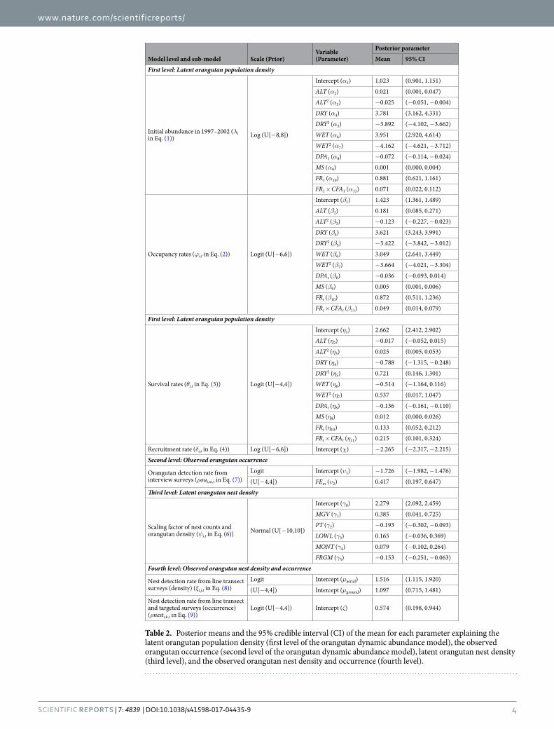
Survey specific parameters. The probability of detecting orangutan nests from field surveys per km2 var-ied depending on respective survey protocol (Table 2). Aerial transects surveys had the highest probability of detecting orangutan nests (logit(1.516)−1 = 82%), followed by the ground transect surveys (75%). This could be because aerial surveys were usually conducted in areas with prior knowledge of orangutan occurrences due to the cost of operating the helicopter. The occurrence data of the combined aerial and ground line transects and other targeted surveys had a lower probability of detecting the nests (64%).

The probability of detecting orangutans via interview surveys was 15% on average if the respondent entered the forest less than once per month and 21% if they entered the forest more frequently (Table 2). The reason for low detection rates of orangutans from interview survey, in comparison to the nests from field survey, is twofold: (1) orangutans are much less common than their nests, and (2) nest count surveys are generally targeted at areas with prior knowledge of orangutan occurrences due to cost constraints.

Nest decay rate was estimated to be 228 days on average for Borneo (Table 2). This however varied slightly across different forest types, where mangrove forest had the longest time to decay (266 days), followed by lowland forest (244 days), montane forest (236 days), and peat forest (209 days).

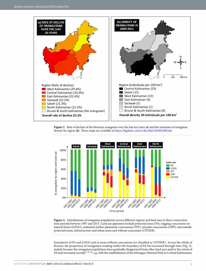
Orangutan abundance by region and land use. The dynamic abundance model estimated that the density of Bornean orangutans has declined by 25% over the last ten years (Fig. 1a). We estimated the overall density of orangutans over Borneo in the period 1997–2002 was about 15 individuals per 100 km2, but the density was reduced to 10 individuals per 100 km2 in 2009–2015 (Supplementary Table 2). We estimated that Central Kalimantan had the highest density of orangutans during 1997–2015, followed by Sabah, West Kalimantan, East Kalimantan, Sarawak, and North Kalimantan (Fig. 1b and Supplementary Table 2).

The distribution of orangutan populations across different land uses varied across regions. In Sabah and Sarawak, most of the orangutan populations resided within the boundaries of protected areas (PA) and log-ging concessions on natural forests (LOGG) (Fig. 2). In Kalimantan, the population generally resided within the

Time period Population range estimates Authors

1961–1970 1,000–4,000 Harrisson71, Schaller72 and Reynolds73

1971–1980 15,000–90,000 Rijksen74

1981–1990 37,000–156,000 MacKinnon75

1991–2000 19,000–65,000 Rijksen & Meijaard11, MacKinnon76 Sugardjito & van Schaik77

2001–2010 54,000–62,675 Wich et al.13 and Singleton et al.78

2011–2015 >100,000 Wich et al.18

Table 1. Total population estimates of the Bornean orangutan (Pongo pygmaeus) made by various authors.

http://1

http://1

http://2

http://2

http://2



Model level and sub-model Scale (Prior)Variable (Parameter)

Posterior parameter

Mean 95% CI

First level: Latent orangutan population density

Initial abundance in 1997–2002 (λi in Eq. (1)) Log (U[−8,8])

Intercept (α1) 1.023 (0.901, 1.151)

ALT (α2) 0.021 (0.001, 0.047)

ALT2 (α3) −0.025 (−0.051, −0.004)

DRY (α4) 3.781 (3.162, 4.331)

DRY2 (α5) −3.892 (−4.102, −3.662)

WET (α6) 3.951 (2.920, 4.614)

WET2 (α7) −4.162 (−4.621, −3.712)

DPA1 (α8) −0.072 (−0.114, −0.024)

MS (α9) 0.001 (0.000, 0.004)

FR1 (α10) 0.881 (0.621, 1.161)

FR1 × CFA1 (α11) 0.071 (0.022, 0.112)

Occupancy rates (ϕi,t in Eq. (2)) Logit (U[−6,6])

Intercept (β1) 1.423 (1.361, 1.489)

ALT (β2) 0.181 (0.085, 0.271)

ALT2 (β3) −0.123 (−0.227, −0.023)

DRY (β4) 3.621 (3.243, 3.991)

DRY2 (β5) −3.422 (−3.842, −3.012)

WET (β6) 3.049 (2.641, 3.449)

WET2 (β7) −3.664 (−4.021, −3.304)

DPAt (β8) −0.036 (−0.093, 0.014)

MS (β9) 0.005 (0.001, 0.006)

FRt (β10) 0.872 (0.511, 1.236)

FRt × CFAt (β11) 0.049 (0.014, 0.079)

First level: Latent orangutan population density

Survival rates (θi,t in Eq. (3)) Logit (U[−4,4])

Intercept (η1) 2.662 (2.412, 2.902)

ALT (η2) −0.017 (−0.052, 0.015)

ALT2 (η3) 0.025 (0.005, 0.053)

DRY (η4) −0.788 (−1.315, −0.248)

DRY2 (η5) 0.721 (0.146, 1.301)

WET (η6) −0.514 (−1.164, 0.116)

WET2 (η7) 0.537 (0.017, 1.047)

DPAt (η8) −0.136 (−0.161, −0.110)

MS (η9) 0.012 (0.000, 0.026)

FRt (η10) 0.133 (0.052, 0.212)

FRt × CFAt (η11) 0.215 (0.101, 0.324)

Recruitment rate (δi,t in Eq. (4)) Log (U[−6,6]) Intercept (χ) −2.265 (−2.317, −2.215)

Second level: Observed orangutan occurrence

Orangutan detection rate from interview surveys (ρoui,m,t in Eq. (7))

Logit Intercept (υ1) −1.726 (−1.982, −1.476)

(U[−4,4]) FEm (υ2) 0.417 (0.197, 0.647)

Third level: Latent orangutan nest density

Scaling factor of nest counts and orangutan density (ψi,t in Eq. (6)) Normal (U[−10,10])

Intercept (γ0) 2.279 (2.092, 2.459)

MGV (γ1) 0.385 (0.041, 0.725)

PT (γ2) −0.193 (−0.302, −0.093)

LOWL (γ3) 0.165 (−0.036, 0.369)

MONT (γ4) 0.079 (−0.102, 0.264)

FRGM (γ5) −0.153 (−0.251, −0.063)

Fourth level: Observed orangutan nest density and occurrence

Nest detection rate from line transect surveys (density) (ξi,j,t in Eq. (8))

Logit Intercept (μaerial) 1.516 (1.115, 1.920)

(U[−4,4]) Intercept (μground) 1.097 (0.715, 1.481)

Nest detection rate from line transect and targeted surveys (occurrence) (ρnesti,k,t in Eq. (9))

Logit (U[−4,4]) Intercept (ζ) 0.574 (0.198, 0.944)

Table 2. Posterior means and the 95% credible interval (CI) of the mean for each parameter explaining the latent orangutan population density (first level of the orangutan dynamic abundance model), the observed orangutan occurrence (second level of the orangutan dynamic abundance model), latent orangutan nest density (third level), and the observed orangutan nest density and occurrence (fourth level).



boundaries of PA and LOGG and in areas without concessions (or classified as ‘OTHER’). Across the whole of Borneo, the proportion of orangutans residing within the boundary of PA has increased through time (Fig. 2), mainly because the orangutan populations have gradually disappeared from other land uses and/or the extent of PA had increased recently9, 10, 20, e.g. with the establishment of the Sebangau National Park in Central Kalimantan,

Figure 1. Rate of decline of the Bornean orangutan over the last ten years (a) and the estimates of orangutan density by region (b). These maps are available at https://figshare.com/s/c8ec56a72628f256b3a8.

Figure 2. Distributions of orangutan populations across different regions and land uses in three consecutive time periods between 1997 and 2015. Land use appraised include protected areas (PA), logging concessions on natural forest (LOGG), industrial timber plantation concessions (ITP), oil palm concessions (OPP), and outside protected areas, infrastructure and urban areas and without concession (OTHER).

https://figshare.com/s/c8ec56a72628f256b3a8



new contiguous protected forests between the Maliau Basin, Imbak Canyon and Danum Valley conservation areas in Sabah, and several new protected areas around the BALE (Batang Ai National Park and Lanjak Entimau Wildlife Reserve) landscapes in Sarawak.

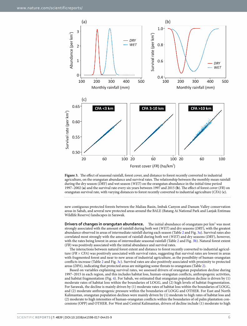
Drivers of changes in orangutan abundance. The initial abundance of orangutans per km2 was most strongly associated with the amount of rainfall during both wet (WET) and dry seasons (DRY), with the greatest abundance observed in areas of intermediate rainfall during each season (Table 2 and Fig. 3a). Survival rates also correlated most strongly with the amount of rainfall during both wet (WET) and dry seasons (DRY), however, with the rates being lowest in areas of intermediate seasonal rainfall (Table 2 and Fig. 3b). Natural forest extent (FR) was positively associated with the initial abundance and survival rates.

The interactions between natural forest extent and distance to forest recently converted to industrial agricul-ture (FR × CFA) was positively associated with survival rates, suggesting that survival rates are lowest in areas with fragmented forest and near to new areas of industrial agriculture, as the possibility of human-orangutan conflicts increase (Table 2 and Fig. 3c). Survival rates are also positively associated with proximity to protected areas (DPA), indicating that protected areas are mitigating some threats to orangutans (Table 2).

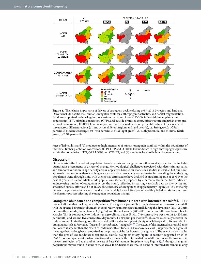
Based on variables explaining survival rates, we assessed drivers of orangutan population decline during 1997–2015 in each region, and this includes habitat loss, human-orangutan conflicts, anthropogenic activities, and habitat fragmentation (Fig. 4). For Sabah, we estimated that orangutan population decline is driven by (1) moderate rates of habitat loss within the boundaries of LOGG, and (2) high levels of habitat fragmentation. For Sarawak, the decline is mainly driven by (1) moderate rates of habitat loss within the boundaries of LOGG, and (2) moderate anthropogenic pressure within the boundaries of LOGG and OTHER. For East and North Kalimantan, orangutan population declines were mainly driven by (1) moderate to high rates of habitat loss and (2) moderate to high intensities of human-orangutan conflicts within the boundaries of oil palm plantation con-cessions (OPP) and OTHER. For West and Central Kalimantan, drivers of decline include (1) moderate to high

Figure 3. The effect of seasonal rainfall, forest cover, and distance to forest recently converted to industrial agriculture, on the orangutan abundance and survival rates. The relationship between the monthly mean rainfall during the dry season (DRY) and wet season (WET) on the orangutan abundance in the initial time period 1997–2002 (a) and the survival rate every six years between 1997 and 2015 (b). The effect of forest cover (FR) on orangutan survival rate, with varying distances to forest recently converted to industrial agriculture (CFA) (c).



rates of habitat loss and (2) moderate to high intensities of human-orangutan conflicts within the boundaries of industrial timber plantation concessions (ITP), OPP and OTHER, (3) moderate to high anthropogenic pressure within the boundaries of ITP, OPP, LOGG and OTHER, and (4) moderate levels of habitat fragmentation.

DiscussionOur analysis is the first robust population trend analysis for orangutans or other great ape species that includes quantitative assessments of drivers of change. Methodological challenges associated with determining spatial and temporal variation in ape density across large areas have so far made such studies infeasible, but our novel approach has overcome these challenges. Our analysis advances current estimates by providing the underlying population trend through time, with the species estimated to have declined at an alarming rate of 25% over the past 10 years. This contradicts crude population estimates proposed by different authors that have indicated an increasing number of orangutans across the island, reflecting increasingly available data on the species and associated survey efforts and not an absolute increase of orangutans (Supplementary Figure 3). This is mainly because the previous studies were conducted separately for each time period and they failed to take into account the dynamic process affecting the orangutan population change.

Orangutan abundance and competition from humans in area with intermediate rainfall. Our model indicates that the long-term abundance of orangutans per km2 is strongly determined by seasonal rainfall, with the species being most abundant in areas receiving intermediate rainfall during the dry season (150–250 mm per month from May to September) (Fig. 3a) and the wet season (200–400 mm per month from November to March). This is comparable to Indonesian agro-climatic zone B with 7–9 consecutive wet months (>200 mm per month) and around two consecutive dry months (<200 mm per month)27. This area essentially receives the right amount of rain throughout the year and is likely able to support plenty of wild tropical fruits essential for orangutans, such as Moraceae (figs) and Anacardiaceae (mangos)38, 39. The extent of the intermediate rainfall zone on Borneo is smaller than the extent of lowlands with altitude <500 m above sea level (Supplementary Figure 4), the range that has long been recognized as the primary niche for Bornean orangutans11. The extent is also smaller than the area of low-moderate mean annual rainfall (Supplementary Figure 4) recently suggested by Wich et al.18. For example, most lowlands in Sarawak are outside the intermediate rainfall zone, as are the lowlands in the western region of Sabah and in the east of East Kalimantan (Supplementary Figure 4). Although orangutan populations may be found in some of these areas, their densities are low. The zone of intermediate rainfall mainly

Figure 4. The relative importance of drivers of orangutan decline during 1997–2015 by region and land use. Drivers include habitat loss, human-orangutan conflicts, anthropogenic activities, and habitat fragmentation. Land uses appraised include logging concessions on natural forest (LOGG), industrial timber plantation concessions (ITP), oil palm concessions (OPP), and outside protected areas, infrastructure and urban areas and without concession (OTHER). Level of importance was assessed based on percentile values of the associated threat across different regions (a), and across different regions and land uses (b), i.e. Strong (red): >75th percentile, Moderate (orange): 50–75th percentile, Mild (light green): 25–50th percentile, and Minimal (dark green): <25th percentile.

http://3

http://4

http://4

http://4



occurs in Central and West Kalimantan, the two provinces with currently the largest orangutan populations outside protected areas. In Sarawak, the zone of intermediate rainfall also occurs around the Batang Ai National Park and Lanjak Entimau Wildlife Reserve, where most of the orangutan populations in this state currently reside.

Besides being important for orangutans, areas with intermediate rainfall are also important for people. The climate in this zone optimally supports plant productivity and agriculture, allowing year-round cultivation of crops, fruits and vegetables27. This is supported by the fact that the proportion of agricultural areas, i.e. planta-tions and agriculture fields and shrublands from abandoned agriculture, outside the government-sanctioned protected areas on Borneo, increases as they are located closer to zones with intermediate rainfall (Supplementary Figure 5d). Because orangutans and humans favor the same climate zone and range, orangutans are facing severe competition from humans, as confirmed by our model where the species survival rates were lowest in this zone (Fig. 3b). In this study we were able to include both altitude and rainfall seasonal pattern as predictors explaining abundance and survival rates because there are no strong correlations between these variables (Supplementary Table 1). Altitude (and its quadratic term) by itself was found to be a non-significant predictor, suggesting that altitude indirectly affects orangutan abundance and survival rates, most likely through rainfall.

While the relationship between rainfall and orangutan abundance is relatively easy to understand from the direct impact of intermediate rainfall on the abundance of wild fruits, the connections between rainfall and orangutan survival rates are more difficult to discern and are most likely related to multifaceted consequences of changing rainfall patterns as part of global climate change and anthropogenic land use change in this area, i.e. vast conversion of forest to agriculture35, 40, 41. Forest clearing has led to the loss of orangutan habitat, as well as the loss of livelihood for communities who greatly depend on forest goods. As climate becomes more erratic, peri-ods of wild fruit scarcity may have increased and the intensity and frequency of forest fires (often originating in drained peat swamp areas) and flooding events (due to upstream deforestation) also increased42, 43. These severe environmental circumstances have most likely led to increased competition between humans and orangutans20. Displaced communities who cannot generate sufficient income from agriculture may seek other income oppor-tunities such as hunting and poaching, or are more sensitive to conflicts with orangutans over crop-raiding44.

The link between areas with intermediate rainfall and hunting propensity can be explained in light of recent research, suggesting that hunting tends to increase with a decrease in forest cover surrounding settlements and an increase in area for agriculture around settlements but a decrease in income from this sector32, 33. Based on population census and land cover data among administrative districts in Kalimantan, we found that districts located within the intermediate rainfall zone have the socio-economic features that lead to higher propensi-ties of hunting compared to districts located outside these zones. The proportions of agricultural areas outside the government-sanctioned protected areas are generally higher in districts where large proportions of these areas overlap with intermediate rainfall range (Supplementary Figure 5a). As anticipated, the proportion of forest areas within the same zones is generally lower in these districts (Supplementary Figure 5b). As the proportions of agricultural areas overlapping with the intermediate rainfall zones in a district increases, the proportion of smallholder farmers decreases (Supplementary Figure 5c) but the proportion of workers engaged in agriculture activities increases (Supplementary Figure 5d). Despite being agriculturally rich, however, the percentage of peo-ple living in poverty is generally higher in these districts that derive lots of their income from industrial-scale agriculture (Supplementary Figure 5e). Also, the poverty-gap index is higher in these agriculturally rich districts (Supplementary Figure 5f), indicating that profits from agricultural development accrue to a small section of society. This indicates that the current orangutan hunting activities could be exacerbated by social and economic circumstances with displaced orangutans competing with small-holder farmers that have less and less land for their own agricultural activities. The connection between socio-economic background, particularly poverty, and hunting and poaching, is generally well known based on various case studies from Asia and Africa39, 45. However, the evidence for claims around poverty as a driver of hunting is weak, mainly because hunting has been over-whelmingly framed exclusively as an issue of conservation and biodiversity loss rather than of poverty and devel-opment46, but that does not mean that poverty is not an important factor.

Recent studies have also found that hunting tends to increase with a decrease of Muslim populations in the village, suggesting that religious affiliation potentially provides a barrier to current orangutan hunting39, 42. Based on census data, we found that agriculturally rich districts located within the intermediate rainfall range in Kalimantan generally have a large proportion of non-Muslim people (Supplementary Figure 5g). This is likely because the high agricultural value has long made these areas the primary home for large indigenous communi-ties, most of which are non-Muslims. Thus, a low proportion of Muslim populations is likely confounded within an area’s high agricultural value, without necessarily influencing the propensity to hunting and orangutan survival rates. Furthermore, our model found a minimal impact of the percentage of Muslims within districts on oran-gutan survival, suggesting a weak correlation between religious affiliation per se and orangutan survival rates. Furthermore, earlier study suggests that hunting for bushmeat is not solely carried out by non-Muslims for their own consumptions, but also by various communities for selling the meat39, implying that the current hunting practices are also driven by economic incentives such as trade. To inform suitable strategies for abating orangutan hunting requires a better understanding of individual hunter motivations, and the anthropological and economic motives driving them47.

Increased contact with humans may also increase the risk of infectious disease in orangutans, which can affect the survival rates of the species in the wild. Previous serological studies suggest that exposure to human patho-gens does occur both in free-ranging and semi-captive orangutans48. Pathogens, such as intestinal parasites, can be transmitted directly from humans49. In rehabilitation centers, overcrowding, abnormality in the population social structure, and dietary imbalances, can exacerbate disease transmission among orangutans48.

Forest, conversion to industrial agriculture, and climate change. Our model indicates that the long-term abundance of orangutans and survival rates per km2 are strongly determined by the extent of natural

http://5d

http://1

http://5a

http://5b

http://5c

http://5d

http://5e

http://5f

http://5g



forest. This suggests that the reduction of forest extent alone will decrease orangutan survival rates. The loss of natural forest was found to be an equally important driver of orangutan declines across all regions of Borneo during 1997–2015 (Fig. 4).

When threats from forest clearing are absent, such as in the case of populations within the boundary of pro-tected areas, survival rates can also decline due to decreasing forest carrying capacity, e.g. increased period of wild fruit scarcity due to climate change. Both global climate change, and climatic changes directly driven by deforestation are predicted to impact rainfall patterns on Borneo, with some areas anticipated to experience sig-nificant rainfall reductions, such as prolonged consecutive dry months50. Isolated forest patches of orangutan hab-itats are particularly prone to extinction due to this type of disturbance. This is exactly the issue currently faced by orangutan populations in Sabah. Comparison among orangutan habitat networks across different regions of Borneo shows that the average size of forest patches where orangutans currently reside are lowest for Sabah (Supplementary Figure 6a) and the distance between forest patches is also largest for this region (Supplementary Figure 6b), suggesting that the populations in this state face the highest risks due to habitat fragmentation (Fig. 4). Hence, although large proportions of orangutan populations in Sabah currently reside within the boundary of PAs, threats from global climate change and other disturbance such as disease, as described earlier, can potentially annihilate orangutan populations within a PA due to relatively small PA size and lack of connectivity among oran-gutans’ habitats within the current PA networks51, 52.

Our model also found that survival rates were determined by the interaction between forest extent and prox-imity to forest recently converted to industrial agriculture. This is likely to be directly related to the increased possibility of human-orangutan conflicts, such as crop-raiding, over newly established large-scale industrial agri-culture and hence killing of crop-raiding individuals53. However, we also found that survival rates increase with proximity to PAs, indicating that forest protection is mitigating some threats to orangutans. Human-orangutan conflicts during 1997–2015 were found to be equally important drivers of orangutan declines across all regions of Borneo (Fig. 4). Although conflicts due to conversion of forest to industrial agriculture appear to occur most intensively in West and Central Kalimantan compared to other regions31, this is probably because large orangutan populations are found in these provinces, and thus does not necessarily imply that conflicts have a relatively min-imal impact on populations in other regions.

Here, we addressed human-orangutan conflicts by assessing the interaction between forest cover and proxim-ity to forest that has been recently converted to industrial agriculture. Conflicts become less frequent with time either because orangutans become less common or adapt to the new landscape54. This is what likely happened in extensive areas of lowland forests in Sabah that had high densities of orangutans prior to the 1960s when the for-ests were converted to oil palm. However, we did not take into account the possibility that the frequency of con-flicts may also vary depending on fruit scarcity. As rainfall is predicted to be more extreme in the future, increased periods of wild fruit shortages are anticipated and this could potentially affect orangutan crop-raiding behavior.

ConclusionOrangutan populations on Borneo have declined at a rate of 25% over the last 10 years. Pressure on orangu-tan populations in the same period of time varied substantially among regions, with the populations in Sabah, Sarawak, East and North Kalimantan experiencing relatively moderate pressure, as opposed to high pressure in West and Central Kalimantan. The co-occurrence of orangutan populations with areas most suitable for human activities has led to an enhanced risk of human-wildlife conflicts. Unless threats from climate change, land use change and other anthropogenic pressure are abated, we predict that most populations of the Bornean orangutan will be severely impacted by human activities.

Poor connectivity among orangutan habitats between the boundaries of PAs is currently the predominant threat to orangutan populations in Sabah. Orangutan populations in Sarawak, East and North Kalimantan face the same threats as West and Central Kalimantan due to habitat loss from continuing forest conversion to indus-trial agriculture and human-orangutan conflicts, but the latter two areas also suffer additionally from anthropo-genic activities.

As the populations in different regions face different threats, specific abatement plans should be implemented to ensure the long-term persistence of the species. This includes (1) maintaining high forest cover in orangu-tan habitats and improving the connectivity among the remaining forest patches where orangutans live through better spatial planning for all regions of Borneo, (2) close cooperation with plantation companies, smallholder farmers and wider communities in managing conflicts with orangutans in Kalimantan, and specifically in West and Central Kalimantan (3) improving the effectiveness of anti-hunting efforts and education and (4) developing a better understanding of the underlying socio-economic motivations of hunting.

MethodsStudy area. Borneo is the third-largest island in the world (approximately 740,000 km2) and is shared by the Malaysian states of Sabah and Sarawak and the sultanate nation of Brunei in the north, and by Indonesian provinces in the south (i.e. West, Central, South and East Kalimantan; the latter was recently divided to establish North Kalimantan province) (Fig. 5a). The island is largely mountainous, with mountains branching westward from the central core along the border between Sarawak and West Kalimantan, and a discontinuous series of mountain ranges running parallel to the east and southeast coasts of the island) (Fig. 5a). Borneo’s interior is largely mountainous but extensive lowlands and swamps occur along the coasts. A large part of Borneo is drained by navigable rivers, which represent the principal and sometimes only routes for trade and commerce, but also present barriers to orangutan dispersal55, 56. The main rivers are the Kapuas in West Kalimantan, the Barito and Kahayan in Central Kalimantan, the Mahakam and Kayan in East Kalimantan, the Rajang and Baram in Sarawak, and the Kinabatangan in Sabah.

http://6a

http://6b


1 0Scientific RepoRts | 7: 4839 | DOI:10.1038/s41598-017-04435-9

We divided Borneo into grid cells with a spatial resolution of 1 × 1 km2, and excluded Brunei and South Kalimantan as they are outside the known orangutan range. This resolution allows us to simulate orangutan dispersal from each focal cell (100 ha) to eight neighboring grid cells, resulting in a 3 × 3 km2 dispersal block (900 ha). This resolution conforms roughly to the home ranges of female Bornean orangutans, which vary between 150 and 850 ha57.

Orangutan data. We utilized two types of orangutan data: nest counts and presence-absence data. The nest count data were obtained from line transect surveys (aerial and ground) (Fig. 5b). The presence-absence data were derived from two survey approaches: (1) line transect (aerial and ground) and targeted surveys of nest observations, and (2) interview surveys of direct orangutan sightings (Fig. 5b). For each survey method, we divided the data into three time periods: (1) 1997–2002, (2) 2003–2008, and (3) 2009–2015, thus providing an analysis of the change in orangutan abundance every six years. This time interval conforms to the minimum inter-birth intervals (the time between consecutive offspring) of female Bornean orangutans58. It also conforms roughly to the time frames of orangutan conservation plans at a national level for Indonesia59 and at state level for Malaysia60.

The aerial survey data mainly cover Sabah and were collected between 1999 and 2012 using helicopters follow-ing different flight routes, as described in Ancrenaz et al.8, 9, giving a total route length of approximately 2,200 km. The ground surveys were carried out sporadically between 1997 and 2015 across Borneo by various orangutan research teams and non-governmental organizations, giving a total transect length of approximately 1,200 km. The targeted surveys mainly include the reconnaissance walks, i.e. a walk following a predetermined direction through the survey area. These surveys followed a standard established methodology to detect and record the nests of great apes3.

To facilitate the use of nest count data collected from various methods of line transect surveys, we standard-ized the metric of orangutan nests to obtain a nest density estimate for each 1 × 1 km2 grid cell. For the ground surveys, we calculated the density of orangutan nests using the Distance sampling method, based on the per-pendicular distance of each nest to the transect12. For the aerial surveys, the data were mainly in the form of an aerial index value (AI) describing the number of nests detected per km of flight. Following Ancrenaz et al.8, the density of orangutan nests per km2, i.e. gnest, can be estimated via: log(gnest) = 4.7297 + 0.9796 log(AI). Density estimates for each 1 × 1 km2 grid cell were then obtained by averaging the estimate across all aerial surveys con-ducted within the grid cell, giving approximately 6,500 of 1 × 1 km2 grid cells where orangutan nest surveys had been conducted across Borneo. These data were then used to form a matrix array of orangutan nest density Yi,j,t comprising three matrices of survey period (t), with each matrix consisting of 6,500 rows of grid cells (i) and 2 columns of survey protocol (j), i.e. ground and aerial transects.

To derive the occupancy of nests in each 1 × 1 km2 grid cell from the ground and aerial transect and targeted surveys for each time period, we first divided the grid into sub-cells with the resolution of 200 × 200 m2. This is to avoid duplicated reports of the same clusters of nests. If at least one survey reported the occurrence of a nest within a sub-cell, we defined that orangutan nests were observed in this sub-cell. If no orangutan nests were recorded within the sub-cell in any of the surveys, we defined that orangutan nests were unobserved in this

Figure 5. Maps of the study area and orangutan surveys. A topographic map of Borneo with regional boundaries and rivers, derived from the SRTM digital elevation data67 district maps provided by the Indonesian Geospatial Information Agency68 and GADM database of Global Administrative Areas69 and river networks provided by the HydroSHEDS70 and visual inspection via Google Earth (a). The locations of orangutan surveys conducted over the last two decades: line transect surveys of orangutan nests (ground and aerial), interview surveys of direct orangutan sightings, and presence points of nest and individual sightings (b). These maps are available at https://figshare.com/s/4ca9f2ae131d6a201751.

https://figshare.com/s/4ca9f2ae131d6a201751



sub-cell. We then constructed a matrix array Znesti,k,t comprising three matrices of survey period (t), and with each matrix comprising 6,500 rows of grid cells (i) and 25 columns of nest observations within sub-cells (k).

The interview surveys of orangutan sightings were conducted in 540 villages across Kalimantan and Sabah in 2008 and 2009, and verification surveys in 2011, with 10 respondents in each village, as described in Meijaard et al.10. Each respondent was asked how frequently he or she entered the forest around the village (i.e. more than once per month or less than once per month) and the last time they had seen an orangutan either in the forest or in the village (i.e. within this year or more than a year ago). Additionally, personal details of each respondent were recorded, including their age and how long they had resided in the village. Based on this information, we derived the occurrence (observed or unobserved) of orangutans in each 1 × 1 km2 grid cell and constructed a matrix array Zoui,m,t, comprising three matrices of survey period (t) with each matrix consisting of 540 rows of grid cells (i) and 10 columns of respondent observations (m). Because the chance of any respondent sighting an orangutan would likely depend on that respondent’s frequency of entering the forest, we also constructed a corresponding binary matrix FEi,m, coded as ‘1’ when respondent m entered the forest around the village in grid cell i more than once a month and ‘0’ when less than once a month.

Dynamic abundance model. The model. We adapted a dynamic population model developed by Chandler & Clark37 for integrating count data and presence-absence data of a species. Our model generalizes the negative binomial model for open populations and assumes that abundance patterns are determined by an initial territory establishment process followed by gains and losses resulting from births, mortalities and dispersal. It also accounts for varying detection errors inherited from different survey data. Our model requires both spatial and temporal data and consists of four broad levels: (1) latent orangutan population density, (2) observed oran-gutan occurrence, (3) latent orangutan nest density, and (4) observed orangutan nest density and occurrence. The first level (latent orangutan population density) can be described as:

Oi,t ~ Bernoulli(ϕi,t) Noui,1 ~ Poisson(λi × Oi,1) Si,t ~ Binomial(Noui,t−1, θi,t) Ri,t ~ Poisson(δi,t) Ñoui,t+1 = Si,t + Ri,t Noui,t+1 ~ Poisson(Ñoui,t+1 × Oi,t+1)

The second level (observed orangutan occurrence) as:

Zoui,m,t ~ Bernoulli(ρoui,m,t × Oi,t)

The third level (latent orangutan nest density) as:

Nnesti,t = ψi,t × Noui,t

Finally, the fourth level (observed orangutan nest density and occupancy) as:

Yi,j,t ~ Binomial(Nnesti,t, ξi,j,t) for nest densityZnesti,k,t ~ Bernoulli(ρnesti,k,t × Onesti,t) for nest occupancy

whereOi,t is the latent occurrence of orangutan at grid cell i in survey period t,Noui,t is the latent number of orangutans at grid cell i in survey period t,Si,t is the latent number of survivors at grid cell i that do not emigrate between period t and t + 1,Ri,t is the latent number of recruits (including births and immigrants) at grid cell i between period t and t + 1,Ñoui,t is the latent number of orangutans at grid cell i in survey period t, as a result of individuals survived and recruited in the previous survey period (Si,t−1 and Ri,t−1, respecitively),Zoui,m,t is the observed orangutan occurrence at grid cell i in survey period t from respondent mNnesti,t is the latent number of orangutan nests at grid cell i in survey period t,Onesti,t is the latent occupancy of orangutan nests at grid cell i in survey period t, derived as a binary value of Nnesti,tYi,j,t is the observed nest count at grid cell i in survey period t from survey type j,Znesti,k,t is the observed nest occurrence at sub-grid cell k and grid cell i in survey period t.

The parameters estimated from the model are the initial abundance rate at grid cell i (λi), survival probability and recruitment rate at grid cell i between survey period t and t + 1 (θi,t and δi,t), the orangutan occupancy rate at grid cell i and survey period t (ϕi,t), the scaling factor of the nest and the orangutan density at grid cell i and sur-vey period t (ψi,t), the probability of detecting orangutan individuals from the interview survey at grid cell i and survey period t for respondent m (ρoui,m,t), the probability of detecting orangutan nests from the line transects at grid cell i and survey period t for survey type j (ξi,j,t, where j ∈ {aerial, ground}), and the probability of detecting orangutan nests from the line transects and other targeted surveys at sub-grid cell k and grid cell i and survey period t (ρnesti,k,t).

These parameters can be modeled by including site-specific covariates. We modeled the initial abundance rate at grid cell i, i.e. λi, as a function of altitude (ALTi), mean annual monthly rainfall during the dry season from May to September (DRYi), mean annual monthly rainfall during the dry season from November to March (WETi), the quadratic term of ALTi, DRYi and WETi, nearest distance to protected areas (DPAi,1), the proportions of Muslims per district (MSi), natural forest extent (FRi,1), and the interaction between natural forest extent and nearest dis-tance to forest recently converted to industrial agriculture (FRi,1 × CFAi,1) that all occurred prior to 2003, i.e.



λ α α α α α α αα α α α

= + + + + + ++ + + + ×

ALT ALT DRY DRY WET WETDPA MS FR FR CFA

log( )( ) (1)

i i i i i i i

i i i i i

1 2 32

4 52

6 72

8 ,1 9 10 ,1 11 ,1 ,1

Natural forest comprised mature natural forest cover that had not been completely cleared in the last 30 years61.The occupancy rate and the survival rate at grid cell i between period t−1 and t, i.e. ϕi,t and θi,t, respectively,

were modeled in a similar manner as the initial abundance rate, i.e.

ϕ β β β β β β

β β β β β

= + + + + +

+ + + + + ×

ALT ALT DRY DRY WET

WET DPA MS FR FR CFA

logit( )

( ) (2)

i t i i i i i

i i t i i t i t i t

, 1 2 32

4 52

6

72

8 , 9 10 , 11 , ,

θ η η η η η η

η η η η η

= + + + + +

+ + + + + ×

ALT ALT DRY DRY WET

WET DPA MS FR FR CFA

logit( )

( ) (3)

i t i i i i i

i i t i i t i t i t

, 1 2 32

4 52

6

72

8 , 9 10 , 11 , ,

We included the quadratic term of ALT, DRY and WET to test the preference of orangutan to occupy areas with intermediate values for altitude and rainfall during the dry and wet season. We also tested whether or not prox-imity to protected areas (DPA) increases survival rates by reducing the risk of orangutan killings. Descriptions of the covariates used to explain the initial abundance, occupancy and survival rates are given in Supplementary Method 1.

The recruitment rate at grid cell i between period t−1 and t, i.e. δi,t, was modeled as the number of individuals in site i and the neighboring sites at the previous survey period62, i.e.

∑δ χ= + =+

+

− −

∈− −NEIGH NEIGH

nw N Nlog( ) log( ) with 1

( 1) (4)i t i t i t

i k nk k t i t, , 1 , 1 , 1 , 1

i

where ni is the first-order neighbours surrounding grid cell i (Moore neighborhood) and wk is a binary indicator (1 or 0) of whether grid cell i is connected to grid cell k ∈ nj. The binary indicator wk was introduced to take into account the effect of large rivers on orangutan dispersal. We used a spatial map of the main rivers in Borneo and determined numerous rivers as barriers to orangutan dispersal, e.g. Kapuas, Barito, Kahayan, Katingan, Rungan, Lamandau, Landak, Mempawah, Mendawai, Paloh, Pawan, Seruyan, Mahakam, Kayan, Rajang, Baram and Kinabatangan. To build wk, we first constructed a vector of straight lines that connect the centre point of grid cell i and the centre point of each adjacent grid cell k ∈ nj

63. This is to simulate the possible dispersal routes taken by an orangutan from grid cell i to the surrounding grid cells. We then intersected this line with the river barrier layer. We assumed wk = 0 if at least one intersection was found within grid cell k ∈ nj (i.e. rivers prevent orangutan dispersal from grid cell i to grid cell k) and wk = 1 if no intersection was found.

In earlier studies, the density of orangutans at grid cell i, i.e. goui, has typically been estimated by the following equation

=× ×

gou gnestb q d (5)

ii

i i i

where bi is the proportion of nest builders, i.e. juveniles less than around 3 years of age are unlikely to build nests64, qi is the daily rate of nest production, and di is the nest decay rate or the number of days a nest remains vis-ible. Based on previous studies in Borneo, the proportion of nest builders has been estimated at around 0.94, 7, 23. The average daily rate of nest production for Bornean orangutans has been estimated to range between 1 and 1.24, 7, 23, but this can fluctuate depending on the level of forest disturbance, i.e. between primary and logged over forest23. Generally, the multiplication of bi and qi results in a value around 1. The nest decay rate is much more uncertain, however, ranging between 85 to over 800 days21–23 and has been shown to vary across different forest types and with altitude4, 7, 23. Hence, to take into account the variability in the total denominator of Eq. (5) across different grid cells i and survey periods t, we modeled ψi,t as

ψ γ γ γ γ γ γ= × + + + + +MGV PT LOWL MONT FRGM100 ( ) (6)i t i t i t i t i t i t, 0 1 , 2 , 3 , 4 , 5 ,

where MGVi,t is a binary variable denoting whether or not the majority of forest at grid cell i and time t are man-grove forest, and similarly PTi,t for peat forest, LOWLi,t for lowland forest (altitude < 500 m), MONTi,t for montane forest (altitude ≥ 500 m), and FRGMi,t for highly fragmented forest (< 25 ha per km2).

The probability of detecting orangutans from the interview surveys at grid cell i and time t for respondent m, i.e. ρoui,m,t, was modeled as a function of respondents’ frequency for entering the forest around the village (1 for more than once a month and 0 for less than once a month), i.e. FEi,m, such that

ρ υ υ= +ou FElogit( ) (7)i m t i m, , 1 2 ,

The probability of detecting orangutan nests at grid cell i and time t and for survey j (j ∈ {aerial, ground}), i.e. ξi,j,t, was modeled constant for each survey type, such that

ξ µ=logit( ) (8)i j t j, ,

http://1



Finally, the probability of detecting orangutan nests at sub-grid cell k and grid cell i and time t for line tran-sects and other targeted surveys, i.e. ρnesti,k,t, was modeled constant, such that

ρ ζ=nestlogit( ) (9)i k t, ,

Model fitting and evaluation. We used WinBUGS Version 1.4.365 to estimate the parameter posterior distribu-tions and the regression coefficients for λi, ϕi,t, θi,t, δi,t, ψi,t, ρoui,m,t, ξi,j,t, and ρnesti,k,t. The WinBUGS code for the dynamic abundance model is provided in Supplementary Method 2. We assumed a vague prior for each param-eter, as described in Table 2.

We ran three Markov chain Monte Carlo (MCMC) chains, where each chain consists of 100,000 iterations and the first 50,000 were discarded as burn-in. To improve convergence and to reduce the autocorrelation in the MCMC chain, we standardized all variables prior to model fitting. Prior to fitting the model to the data, we tested the correlation among the original (unstandardized) environmental variables explaining λ, ϕt and θt, i.e. variables ALT, DRY, WET, DPA, MS, FR and CFA, and also among the standardized variables. Convergence for each model parameter was assessed from the values of Rhat statistics and visualization of the chain plot of the MCMC itera-tions. Rhat values around 1 and the absence of seasonality within each chain plot and overlap among the chains indicate convergence. We also tested for correlations among posterior distributions of the coefficients, especially between the linear and the quadratic terms of variables ALT, DRY and WET, to ensure correct functional forms were specified for these variables and the coefficients were not biased.

The goodness-of-fit of the model was assessed by comparing the simulated nest abundance predictions for each time period with the observed nest counts. For each simulated prediction and time period, we calculated the Pearson’s correlation coefficient r and also fitted a linear regression between the predicted values and the observed values to calculate the R2 value66. We also validated the simulated orangutan presence-absence predictions for each time period against the actual observations based on interview surveys. In the validation dataset, we defined “presence” in a village if at least one respondent reported the occurrence of orangutan, and we defined “absence” if more than 50% of the respondents who enter the forest more than once a month had never seen the species. We used the proportions of correctly predicted presence or Sensitivity (SN) and the proportions of correctly predicted absence or Specifity (SP) as the measure of performance. SN and SP values close to one indicate high accuracy.

Assessing orangutan abundance change among regions and land uses. We assessed orangutan population trends by measuring the change in the number of individuals obtained from the simulated predictions. We investigated how the trends vary across different regions (states and provinces), as well as across different land uses. We con-sidered five land use categories: (1) protected areas (PA), (2) logging concessions on natural forests (LOGG), (3) industrial timber plantation concessions (ITP), (4) oil palm plantation concessions (OPP), and (5) outside pro-tected areas, infrastructure and urban areas and without concessions, mostly small-scale agriculture and smaller forest patches (OTHER). We obtained spatial boundary data for protected areas, logging concessions, timber plantation concessions, and oil palm concessions for Kalimantan, Sabah and Sarawak for 2000, 2006 and 2012 from various sources (see Supplementary Method 3).

Assessing drivers of orangutan population decline among regions and land uses. To inform orangutan conserva-tion planning, we assessed the drivers of orangutan population decline in each region. This was achieved mainly by relating the environmental covariates explaining survival rates in Eq. (3) across 1 × 1 km2 grid cells where orangutans are predicted to occur with known actual threats observed on Borneo. These threats includes: (1) habitat loss, i.e. the loss of natural forest of orangutan habitats, (2) human-orangutan conflicts, (3) anthropogenic human activities, such as hunting and poaching, and (4) habitat fragmentation, i.e. breaking up intact forest hab-itats into small forest patches.

The decline of orangutan population due to habitat loss in grid cell i at time period t, i.e. HLOSSi,t, was related specifically to forest cover covariate FRi,t (i.e. the 10th additive component in Eq. (3)). We measured habitat loss based on counterfactual analysis, i.e. the discrepancy between the survival rates under the ‘counterfactual assumption of no forest loss, or forest cover remains the same as in the previous time period (FRi,t−1)’ versus ‘the actual forest cover in that period (FRi,t)’, such that

= −−HLOSS FR FRi t i t i t, , 1 ,

High HLOSSi,t implies low orangutan survival rate, or high contribution of habitat loss to population decline in grid cell i at time period t.

The decline of orangutan population due to human-orangutan conflicts in grid cell i at time period t, i.e. CONFLi,t, was related specifically to the interaction between forest cover FRi,t and the distance to newly converted forest to industrial agriculture CFAi,t (i.e. the 11th additive component in Eq. (3)), such that

= ×CONFL FR CFAi t i t i t, , ,

Low CONFLi,t implies low orangutan survival rate, or high contribution of human-orangutan conflicts to popu-lation decline in grid cell i at time period t.

For measuring the decline of orangutan population due to anthropogenic activities in grid cell i at time period t, i.e. ANTHi,t, we used monthly rainfall during the dry DRYi and the wet seasons WETi and proximity to pro-tected areas DPAi,t as proxy (i.e. 4–8th additive components in Eq. (3)), such that

http://2

http://3



η η η η η= + + + +ˆ ˆ ˆ ˆ ˆANTH DRY DRY WET WET DPAi t i i i i i t, 4 52

6 72

8 ,

where η η η η ηˆ ˆ ˆ ˆ ˆ, , , , and4 5 6 7 8 are the estimated coefficients obtained from WinBUGS simulations. This is because seasonal rainfall patterns determine socio-economic structure and livelihoods on Borneo34. Additionally, pro-tected areas were assumed to provide a refuge for the species against hunting and poaching11. Low ANTHi,t implies low orangutan survival rate, or high contribution of anthropogenic activities to population decline in grid cell i at time period t.

To obtain the relative influence of habitat loss as a driver of orangutan population decline for each region, we averaged HLOSSi,t across all grid cells where orangutans are predicted to occur within the respective region. To obtain the relative influence of human-orangutan conflicts and anthropogenic activities as drivers of population decline for each region, we applied similar procedure to CONFLi,t and ANTHi,t, respectively. We also assessed how these drivers vary across different land uses (i.e. LOGG, ITP, OPP and OTHER) within each region.

For habitat fragmentation, we assessed this as a driver over the entire orangutan distribution range across dif-ferent landscapes within the region. Because territorial ranges of orangutans, especially the females, are generally restricted to a maximum of 850 ha55, the species’ dispersal opportunities between habitat fragments are generally limited. This implies that landscapes with isolated forest patches of orangutan habitats (i.e. fragmented habitats) have a higher risk of orangutan decline due to lower colonization rates than landscapes with better habitat con-nectivity. The relative influence of habitat fragmentation as a driver of orangutan population decline in a region, i.e. FRAG, was estimated as the interaction between the mean size of contiguous forest where orangutan occurred and the mean reciprocal distance of each contiguous forest to the nearest forest patch. Low FRAG implies low orangutan survival rate, or high contribution of habitat fragmentation to population decline.

References 1. Ancrenaz, M. et al. Pongo pygmaeus ssp. pygmaeus. The IUCN Red List of Threatened Species 2016, e.T39781A17990445 (2016). 2. Meijaard, E., Wich, S., Ancrenaz, M. & Marshall, A. J. Not by science alone: why orangutan conservationists must think outside the

box. Ann. N. Y. Acad. Sci. 1249, 29–44 (2012). 3. Kühl, H., Maisels, F., Ancrenaz, M. & Williamson, L. Best Practice Guidelines for the Surveys and Monitoring of Great Ape Populations.

Gland, Switzerland: IUCN/SSC Primate Specialist Group (2008). 4. van Schaik, C. P., Priatna, A. & Priatna, D. In Population Estimates and Habitat Preferences of Orangutans Based on Line Transects of

Nests: The Neglected Ape (eds Nadler, R. D.) 129–147 (Springer US, 1995). 5. Russon, A. E., Erman, A. & Dennis, R. The population and distribution of orangutans (Pongo pygmaeus pygmaeus) in and around

the Danau Sentarum Wildlife Reserve, West Kalimantan, Indonesia. Biol. Conserv. 97, 21–28 (2001). 6. Ancrenaz, M., Goossens, B., Gimenez, O., Sawang, A. & Lackman-Ancrenaz, I. Determination of ape distribution and population

size using ground and aerial surveys: a case study with orang-utans in lower Kinabatangan, Sabah, Malaysia. Anim. Conserv. 7, 375–385 (2004).

7. Johnson, A. E., Knott, C. D., Pamungkas, B., Pasaribu, M. & Marshall, A. J. A survey of the orangutan (Pongo pygmaeus wurmbii) population in and around Gunung Palung National Park, West Kalimantan, Indonesia based on nest counts. Biol. Conserv. 121, 495–507 (2005).

8. Ancrenaz, M. et al. Aerial surveys give new estimates for orangutans in Sabah, Malaysia. PLoS Biol. 3, e3 (2005). 9. Ancrenaz, M. et al. Recent surveys in the forests of Ulu Segama Malua, Sabah, Malaysia, show that orangutans (P. p. morio) can be

maintained in slightly logged forests. PLoS One 5, e11510 (2010). 10. Meijaard, E. et al. Why don’t we ask? A complementary method for assessing the status of great apes. PLoS One 6, e18008 (2011). 11. Rijksen, H. D. & Meijaard, E. Our Vanishing Relative: The Status of Wild Orang-utan at the Close of the Twentieth Century (Kluwer

Academic Publishers, 1999). 12. Buckland, S. T., Anderson, D. R., Burnham, K. P. & Laake, J. L. Distance Sampling (John Wiley & Sons Ltd, 2005). 13. Wich, S. A. et al. Distribution and conservation status of the orang-utan (Pongo spp.) on Borneo and Sumatra: how many remain?

Oryx 42, 329–339 (2008). 14. Knop, E., Ward, P. I. & Wich, S. A. A comparison of orang-utan density in a logged and unlogged forest on Sumatra. Biol. Conserv.

120, 183–188 (2004). 15. Wich, S. A., Buij, R. & Van Schaik, C. Determinants of orangutan density in the dryland forests of the Leuser Ecosystem. Primates

45, 177–182 (2004). 16. Friedman, J. H., Hastie, T. & Tibshirani, R. Additive logistic regression: a statistical view of boosting. Ann. Stat. 28, 337–407 (2000). 17. Phillips, S. J. & Dudík, M. Modeling of species distributions with Maxent: new extensions and a comprehensive evaluation.

Ecography 31, 161–175 (2008). 18. Wich, S. A. et al. Understanding the impacts of land-use policies on a threatened species: is there a future for the Bornean orang-

utan? PLoS One 7, e49142 (2012). 19. Gregory, S. D. et al. Long-term field data and climate-habitat models show that orangutan persistence depends on effective forest

management and greenhouse gas mitigation. PLoS One 7, e43846 (2012). 20. Struebig, M. J. et al. Anticipated climate and land‐cover changes reveal refuge areas for Borneo’s orang‐utans. Glob. Chang. Biol. 21,

2891–2904 (2015). 21. Marshall, A. J. & Meijaard, E. Orangutan nest surveys: the devil is in the details. Oryx 43, 416–418 (2009). 22. Mathewson, P., Spehar, S., Meijaard, E., Sasmirul, A. & Marshall, A. Evaluating orangutan census techniques using nest decay rates:

implications for population estimates. Ecol. Appl. 18, 208–221 (2008). 23. Ancrenaz, M., Calaque, R. & Lackman-Ancrenaz, I. Orangutan nesting behavior in disturbed forest of Sabah, Malaysia: implications

for nest census. Int. J. Primatol. 25, 983–1000 (2004). 24. Husson, S. J. et al. In Orangutan Distribution, Density, Abundance and Impacts of Disturbance: Orangutans: Geographic Variation in

Behavioral Ecology and Conservation (eds Wich, S., Utami, S., Setia, T. & van Schaik, C.) 77–96 (Oxford University Press, 2009). 25. Wich, S. A. & van Schaik, C. P. The impact of El Niño on mast fruiting in Sumatra and elsewhere in Malesia. J. Trop. Ecol. 16,

563–577 (2000). 26. Regional Physical Planning Programme for Transmigration (RePPProT). Review of Phase 1. Main Report. Land Resources

Department ODNRI, Overseas Development Administrator (London, UK and Departement of Transmigration, Jakarta, Indonesia, 1991).

27. Oldeman, L. R. & Frere, M. Technical Report on a Study of the Agroclimatology of the Humid Tropics of Southeast Asia (Food & Agriculture Organization (FAO), Rome, Italy, 1982).

28. Goossens, B. et al. Genetic signature of anthropogenic population collapse in orang-utans. PLoS Biol. 4, 285 (2006).



29. Meijaard, E. et al. Declining orangutan encounter rates from Wallace to the present suggest the species was once more abundant. PLoS One 5, e12042 (2010).

30. Marshall, A. J. et al. The blowgun is mightier than the chainsaw in determining population density of Bornean orangutans (Pongo pygmaeus morio) in the forests of East Kalimantan. Biol. Conserv. 129, 566–578 (2006).

31. Meijaard, E. et al. Quantifying killing of orangutans and human-orangutan conflict in Kalimantan, Indonesia. PLoS One 6, e27491 (2011).

32. Davis, J. T. et al. It’s not just conflict that motivates killing of orangutans. PLoS One 8, e75373 (2013). 33. Abram, N. K. et al. Mapping perceptions of species’ threats and population trends to inform conservation efforts: the Bornean

orangutan case study. Divers. Distrib. 21, 487–499 (2015). 34. Gaveau, D. L. et al. Reconciling forest conservation and logging in Indonesian Borneo. PLoS One 8, e69887 (2013). 35. Santika, T., Meijaard, E. & Wilson, K. A. Designing multifunctional landscapes for forest conservation. Environ. Res. Lett. 10, 114012

(2015). 36. Meijaard, E. et al. Life After Logging: Reconciling Wildlife Conservation and Production Forestry in Indonesian Borneo (CIFOR and

UNESCO, Jakarta, 2005). 37. Chandler, R. B. & Clark, J. D. Spatially explicit integrated population models. Methods Ecol. Evol. 5, 1351–1360 (2014). 38. Campbell-Smith, G., Sembiring, R. & Linkie, M. Evaluating the effectiveness of human-orangutan conflict mitigation strategies in

Sumatra. J. Appl. Ecol. 49, 367–375 (2012). 39. Smith, R. J., Muir, R. D. J., Walpole, M. J., Balmford, A. & Leader-Williams, N. Governance and the loss of biodiversity. Nature 426,

67–70 (2003). 40. Gaveau, D. L. A. et al. Rapid conversions and avoided deforestation: examining four decades of industrial plantation expansion in

Borneo. Sci. Rep. 6, 32017 (2016). 41. Gaveau, D. L. A. et al. Four decades of forest persistence, loss and logging on Borneo. PLoS One 9, e101654 (2014). 42. Langner, A., Miettinen, J. & Siegert, F. Land cover change 2002–2005 in Borneo and the role of fire derived from MODIS imagery.

Glob. Chang. Biol. 13, 2329–2340 (2007). 43. Wells, J. A. et al. Rising floodwaters: mapping impacts and perceptions of flooding in Borneo. Environ. Res. Lett. 11, 064016 (2016). 44. Campbell-Smith, G., Campbell-Smith, M., Singleton, I. & Linkie, M. Raiders of the Lost Bark: Orangutan Foraging Strategies in a

Degraded Landscape. PLoS One 6, e20962 (2011). 45. Burn, R. W., Underwood, F. M. & Blanc, J. Global trends and factors associated with the illegal killing of elephants: a hierarchical

bayesian analysis of carcass encounter data. PLoS One 6, e24165 (2011). 46. Kaimowitz, D. & Sheil, D. Conserving what and for whom? Why conservation should help meet basic human needs in the tropics.

Biotropica 39, 567–574 (2007). 47. Ostrom, E., Burger, J., Field, C. B., Norgaard, R. B. & Policansky, D. Revisiting the commons: local lessons, global challenges. Science

284, 278–282 (1999). 48. Kilbourn, A. M. et al. Health evaluation of free-ranging and semi-captive orangutans (Pongo pygmaeus pygmaeus) in Sabah,

Malaysia. J. Wildl. Dis. 39, 73–83 (2003). 49. Labes, E. M. et al. Intestinal parasites of endangered orangutans (Pongo pygmaeus) in Central and East Kalimantan, Borneo,

Indonesia. Parasitology 137, 123–135 (2010). 50. Struebig, M. J. et al. Targeted conservation to safeguard a biodiversity hotspot from climate and land-cover change. Curr. Biol. 25,

372–378 (2015). 51. Gregory, S. D. et al. Forecasts of habitat suitability improve habitat corridor efficacy in rapidly changing environments. Divers.

Distrib. 9, 1044–1057 (2014). 52. Gregory, S. D. et al. Long-term field data and climate-habitat models show that orangutan persistence depends on effective forest

management and greenhouse gas mitigation. PloS One 7, e43846 (2012). 53. Ancrenaz, M., Dabek, L. & O’Neil, S. The cost of exclusion: recognizing a role for local communities in biodiversity conservation.

PLoS Biol. 5, e289 (2007). 54. Ancrenaz, M. et al. Of pongo, palms, and perceptions – A multidisciplinary assessment of orangutans in an oil palm context. Oryx

49, 465–472 (2015). 55. Jalil, M. F. et al. Riverine effects on mitochondrial structure of Bornean orang-utans (Pongo pygmaeus) at two spatial scales. Mol.

Ecol. 17, 2898–2909 (2008). 56. Arora, N. et al. Effects of Pleistocene glaciations and rivers on the population structure of Bornean orangutans (Pongo pygmaeus).

Proc. Natl. Acad. Sci. USA. 107, 21376–21381 (2010). 57. Singleton, I., Knott, C. D., Morrogh-Bernard, H. C., Wich, S. A. & van Schaik, C. P. In Ranging Behavior of Orangutan Females and

Social Organization: Orangutans: Geographic Variation in Behavioral Ecology and Conservation (eds Wich, S., Utami, S., Setia, T. & van Schaik, C.) 205–213 (Oxford University Press, 2009).

58. Knott, C. D., Thompson, M. E. & Wich, S. A. In The Ecology of Reproduction in Wild Orangutans: Geographic Variation in Behavioral Ecology and Conservation (eds Wich, S., Utami, S., Setia, T. & van Schaik, C.) 171–188 (Oxford University Press, 2009).

59. Ministry of Forestry Indonesia. Orangutan Indonesia: Conservation Strategies and Action Plan 2007–2017 (Jakarta, Indonesia, 2009). 60. Sabah Wildlife Department. Orangutan Action Plan 2012–2016 (Kota Kinabalu, Sabah, Malaysia, 2011). 61. Margono, B. A., Potapov, P. V., Turubanova, S., Stolle, F. & Hansen, M. C. Primary forest cover loss in Indonesia over 2000–2012. Nat.

Clim. Change 4, 730–735 (2014). 62. Besag, J. Spatial interaction and the statistical analysis of lattice systems. J. R. Stat. Soc. Series B Stat. Methodol. 36, 192–236 (1974). 63. Santika, T., McAlpine, C. A., Lunney, D., Wilson, K. A. & Rhodes, J. R. Assessing spatio-temporal priorities for species’ recovery in

broad-scale dynamic landscapes. J. Appl. Ecol. 52, 832–840 (2015). 64. Prasetyo, D. et al. In Nest Building in Orangutans: Geographic Variation in Behavioral Ecology and Conservation (ed. Wich, S., Utami,

S., Setia, T. & van Schaik, C.) 269–277 (Oxford University Press, 2009). 65. Lunn, D. J., Thomas, A., Best, N. & Spiegelhalter, D. WinBUGS-a Bayesian modelling framework: concepts, structure, and

extensibility. Stat. Comput 10, 325–337 (2000). 66. Bahn., V. & McGill, B. J. Testing the predictive performance of distribution models. Oikos 122, 321–331 (2013). 67. Jarvis, A., Reuter, H. I., Nelson, A. & Guevara, E. Hole-filled SRTM for the Globe Version 4 Available at http://srtm.csi.cgiar.org

(accessed 21 December 2015) (2008). 68. Geospatial Information Agency Indonesia. Provincial Map. Available at http://www.big.go.id/peta-provinsi (accessed 10 October

2015) (2014). 69. Global Administrative Areas. GADM Database of Global Administrative Areas Version 2.0. Available at http://www.gadm.org

(accessed 2 October 2015) (2012). 70. Lehner, B., Verdin, K. & Jarvis, A. New global hydrography derived from spaceborne elevation data. Eos. Trans. AGU 89, 93–94.

Available at http://hydrosheds.cr.usgs.gov (accessed 15 November 2015) (2008). 71. Harrisson, B. Orang Utan: What chances of survival. Sarawak Mus. J 10, 238–261 (1961). 72. Schaller, G. B. The orangutan in Sarawak. Zoologica 46, 73–82 (1961). 73. Reynolds, V. A. The Apes. The Gorilla, Chimpanzee, Orangutan, and Gibbon. Their History and Their World (Harper & Row New

York, 1967).

http://www.big.go.id/peta-provinsi

http://www.gadm.org

http://hydrosheds.cr.usgs.gov



74. Rijksen, H. D. A Fieldstudy on Sumatran Orangutans (Pongo pygmaeus abelii Lesson 1827). Ecology, Behaviour and Conservation (Nature Conservation Department, Agricultural University Wageningen, Wageningen, The Netherlands, 1978).

75. MacKinnon, K. In The Conservation Status of Nonhuman Primates in Indonesia: Primates, The Road to Self-Sustaining Populations (eds Benirschke, K.) 99–126 (Springer Verlag, New York, United States of America, 1986).

76. MacKinnon, J. In Species Survival Plan for the Orangutan: Forest Biology and Conservation in Borneo (eds Ismail, G., Mohamed, M. & Omar, S.) 209–219 (Center for Borneo Studies Publication, 1992).

77. Sugardjito, J. & van Schaik, C. P. In Orangutans: Current Population Status, Threats, and Conservation Measures: Proceedings of the Conservation of the Great Apes in the New World Order of the Environment. 142–152 (Ministry of Forestry and Tourism, Post and Telecommunications, Republic of Indonesia, 1992).

78. Singleton, I. et al. Orangutan Population and Habitat Viability Assessment: Final Report (IUCN/SSC Conservation Breeding Specialist Group, Apple Valley, MN, USA, 2004).

AcknowledgementsThis study is part of “Borneo Futures” initiative. Funding for this collaborative work is provided in the Supplementary Data. We are greatly indebted to all orangutan researchers and wildlife personnel whose efforts were valuable in data collection, and for making this study possible. We also thank the governments of Indonesia and Malaysia, and their forest and environmental departments, for supporting this research.

Author ContributionsT.S., K.A.W., S.S., E.M., and M.A. conceived the study; T.S. compiled the environmental data and conducted the modeling; T.S., K.A.W., S.S., E.M., and M.A. interpreted the results; T.S. wrote the manuscript, which was revised by K.A.W., S.S., E.M., M.A., G.L.B., H.H., J.W., K.M., f.M., N.A., N.M., M.V., S.A.W. & S.S.U.A.; S.S., E.M., M.A., A.H.S., A.P., A.T., A.S., A.E., A.J.M., A.R., A.E.R., A.N., A.M., A.L., B.G., C.P.S., D.R., D.P., E.S., E.P.W., G.C.S., G.L.B., H.K., I.S., I.L., J.S., K.L., K.O., L.A., L.C., M.V., M.H., N., N.A.P., R.A.D., S.A.W., S.J.H., S.R. & S.S.U.A. collected the underlying data.

Additional InformationSupplementary information accompanies this paper at doi:10.1038/s41598-017-04435-9Competing Interests: The authors declare that they have no competing interests.Publisher's note: Springer Nature remains neutral with regard to jurisdictional claims in published maps and institutional affiliations.

Open Access This article is licensed under a Creative Commons Attribution 4.0 International License, which permits use, sharing, adaptation, distribution and reproduction in any medium or

format, as long as you give appropriate credit to the original author(s) and the source, provide a link to the Cre-ative Commons license, and indicate if changes were made. The images or other third party material in this article are included in the article’s Creative Commons license, unless indicated otherwise in a credit line to the material. If material is not included in the article’s Creative Commons license and your intended use is not per-mitted by statutory regulation or exceeds the permitted use, you will need to obtain permission directly from the copyright holder. To view a copy of this license, visit http://creativecommons.org/licenses/by/4.0/. © The Author(s) 2017

http://dx.doi.org/10.1038/s41598-017-04435-9

http://creativecommons.org/licenses/by/4.0/

Date post:	04-Apr-2019
Category:	Documents
Upload:	lycong
View:	217 times
Download:	0 times

First integrative trend analysis for a great ape species...

Documents