First-principles calculations for point defects in solids
Christoph Freysoldt, Blazej Grabowski, Tilmann Hickel, and Jörg Neugebauer
Max-Planck-Institut für Eisenforschung GmbH, D-40237 Düsseldorf, Germany
Georg Kresse
University of Vienna, Faculty of Physics and Center for Computational Materials Science,A-1090 Wien, Austria
Anderson Janotti and Chris G. Van de Walle
Materials Department, University of California, Santa Barbara, California 93106-5050, USA
(published 28 March 2014)
Point defects and impurities strongly affect the physical properties of materials and have a decisiveimpact on their performance in applications. First-principles calculations have emerged as apowerful approach that complements experiments and can serve as a predictive tool in theidentification and characterization of defects. The theoretical modeling of point defects incrystalline materials by means of electronic-structure calculations, with an emphasis on approachesbased on density functional theory (DFT), is reviewed. A general thermodynamic formalism is laiddown to investigate the physical properties of point defects independent of the materials class(semiconductors, insulators, and metals), indicating how the relevant thermodynamic quantities,such as formation energy, entropy, and excess volume, can be obtained from electronic structurecalculations. Practical aspects such as the supercell approach and efficient strategies to extrapolateto the isolated-defect or dilute limit are discussed. Recent advances in tractable approximations tothe exchange-correlation functional (DFTþU, hybrid functionals) and approaches beyond DFT arehighlighted. These advances have largely removed the long-standing uncertainty of defectformation energies in semiconductors and insulators due to the failure of standard DFT toreproduce band gaps. Two case studies illustrate how such calculations provide new insight into thephysics and role of point defects in real materials.
I. Introduction 254A. Role of point defects and impurities in solids 255
1. Doping 2552. Overcoming doping limits and achieving
ambipolar doping 255a. Solubility 256b. Ionization energy 256c. Incorporation of impurities in other
configurations 256d. Compensation by native point defects 256e. Compensation by foreign impurities 256
3. Diffusion 2564. Thermodynamics and phase stability 257
B. Key quantities 2571. Formation energies 2572. Complex formation and binding energies 2583. Charge-state transition levels in semiconductors
and insulators 2594. Quantities amenable to comparison
with experiment 259a. Defect concentrations 259b. Atomic structure 260c. Scanning tunneling microscopy and
spectroscopy 260d. g factors and hyperfine parameters 260
e. NMR chemical shifts 260f. Mössbauer spectroscopy 260g. Vibrational frequencies 260h. Defect transition levels 261
C. Requirements for theoretical andcomputational treatments 2611. Electronic-structure approaches 2612. Constraints on accuracy of computational results 261
II. Thermodynamic Concepts 262A. Entropy of defects 262
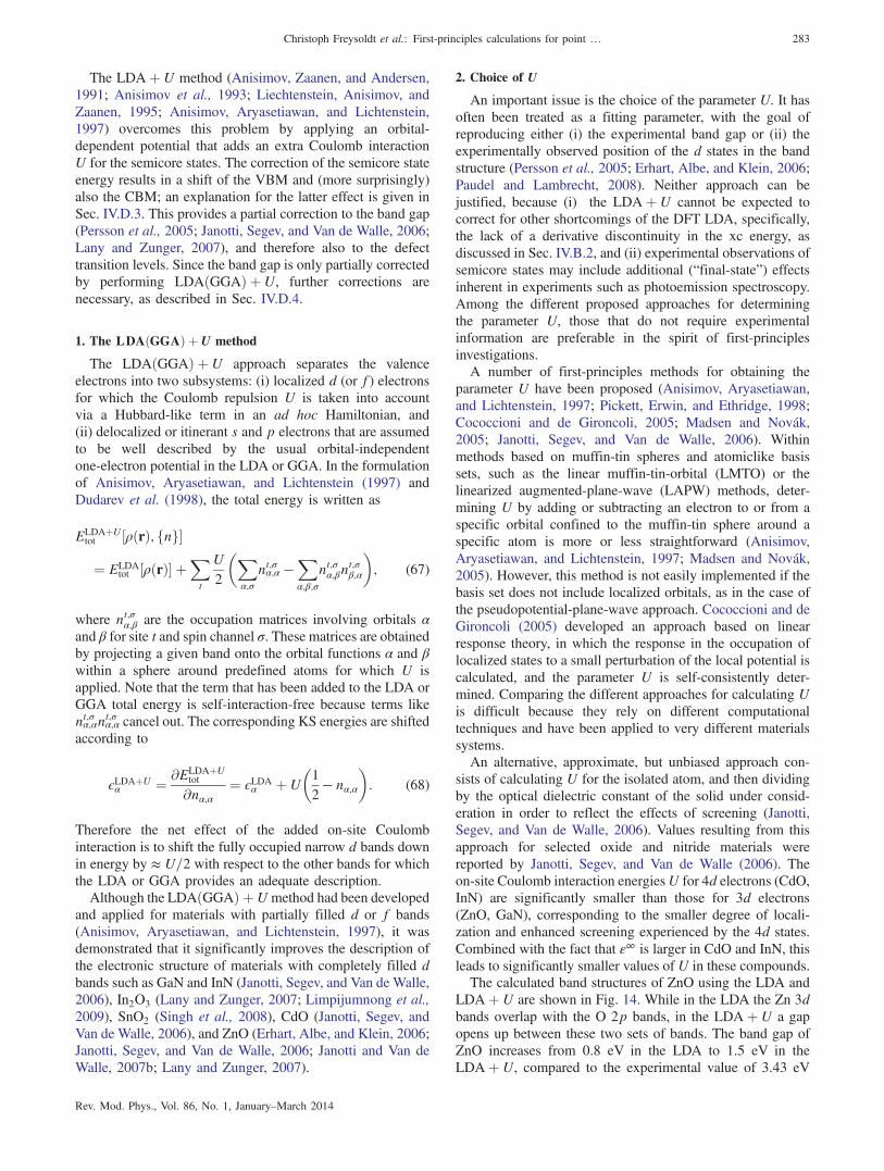
2. Effect of xc errors on defect formation energies 269D. Thermodynamic transition levels 269
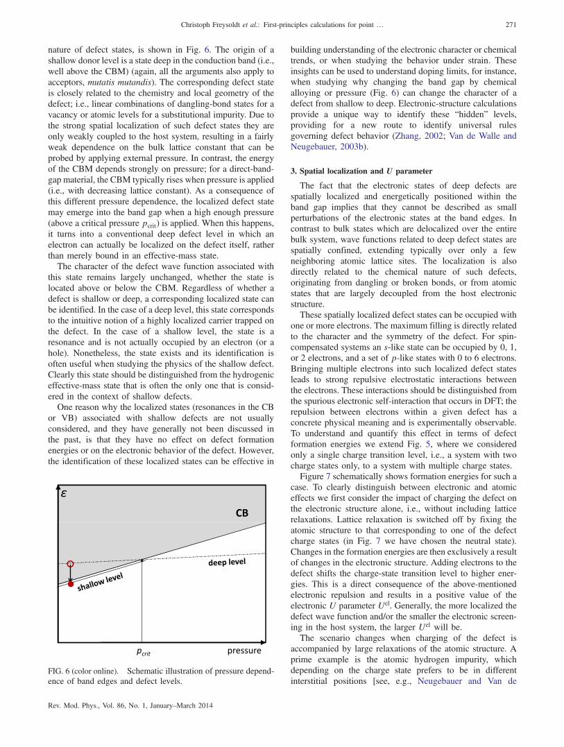
1. Deep levels 2702. Shallow levels 2703. Spatial localization and U parameter 271
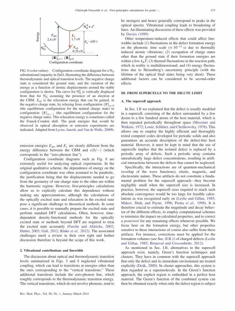
E. Optical transition levels 2721. Configuration coordinate diagrams 2722. Vibrational contributions and linewidth 273
III. From Supercells to the Dilute Limit 273A. The supercell approach 273B. Overlap of wave functions 274
1. Dispersion of the defect band 2742. Partially occupied states 2743. Corrections for shallow levels 275
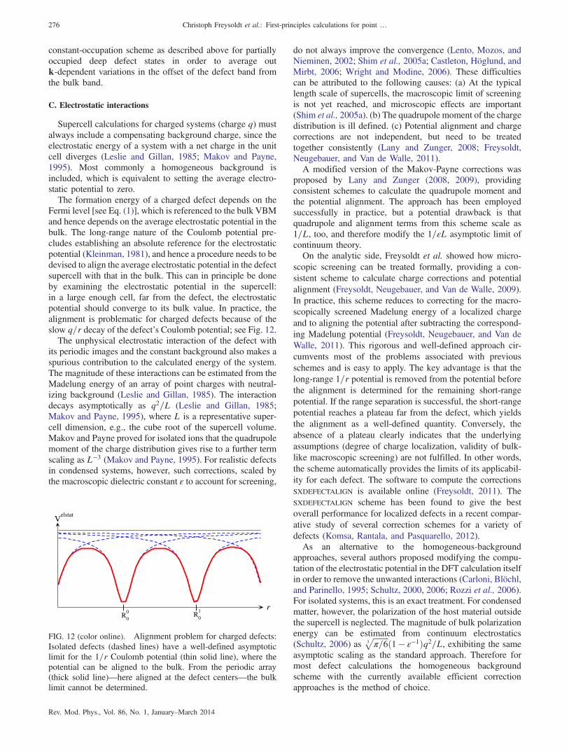
C. Electrostatic interactions 276D. Elastic interactions 277E. Magnetic interactions 277F. Recommendations 278
IV. Overcoming the Band-gap Problem 278A. Hartree-Fock theory 279B. Shortcomings of density functional theory 279
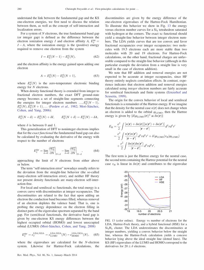
1. Self-interaction and localization errors 2792. Exchange-correlation derivative discontinuity 281
C. Extrapolation schemes 281D. LDAðGGAÞ þU for materials with
semicore d states 2821. The LDAðGGAÞ þU method 2832. Choice of U 2833. Band alignment between LDA and LDAþ U 2844. Corrected defect transition levels and formation
energies based on LDAþU 284E. Correction schemes based on modification
of pseudopotentials 2861. Self-interaction-corrected pseudopotentials 2862. Modified pseudopotentials 286
F. Quasiparticle calculations 2871. Fundamental concepts 2872. Practical approximations 2883. Self-consistency and vertex corrections 2894. Constraints and limitations 290
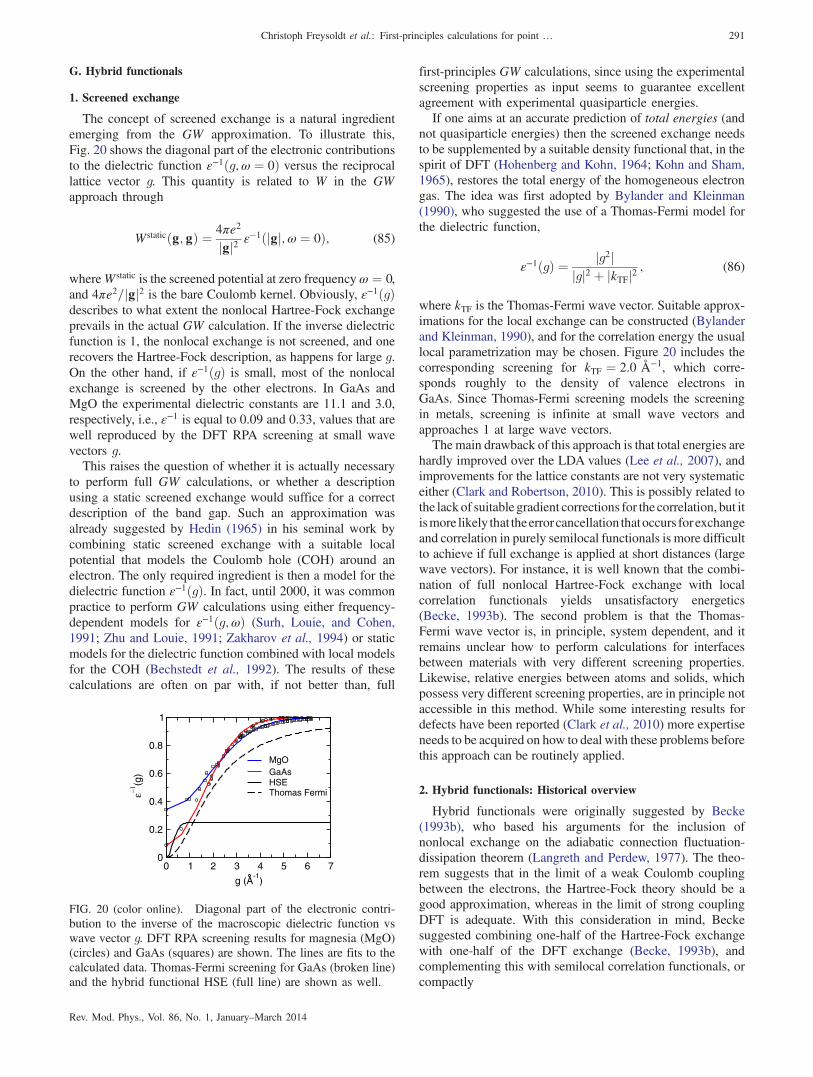
G. Hybrid functionals 2911. Screened exchange 2912. Hybrid functionals: Historical overview 2913. The incentive to use hybrid functionals and 1=4
of the exact exchange 2924. Performance of hybrid functionals 293
H. Quantum Monte Carlo calculations 294V. Case Studies 294
A. Overcoming doping limits 2941. Causes of unintentional n-type conductivity
in ZnO 295a. Native point defects 295b. Impurities 296
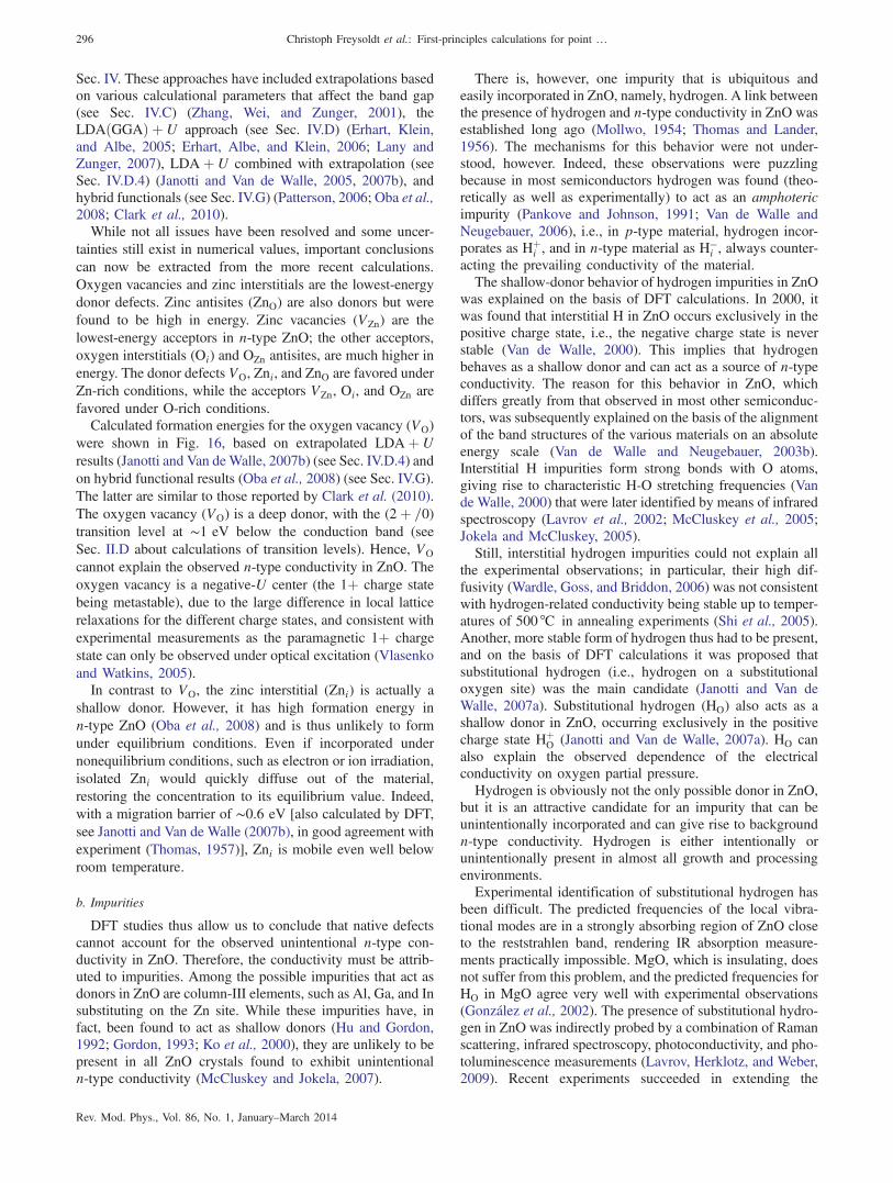
2. p-type doping of ZnO 297B. Impact of point defects on phase stability close
to the melting temperature 2971. The debate about vacancies versus
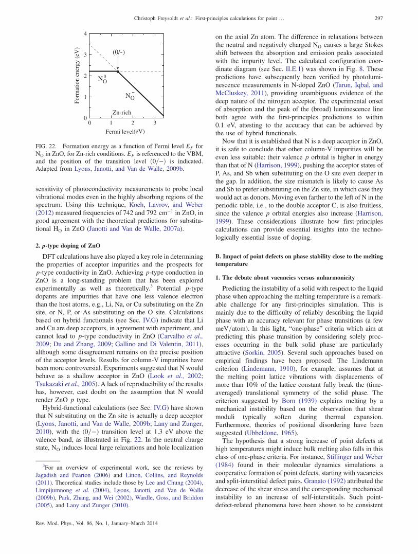
anharmonicity 2972. First-principles studies for Al 298
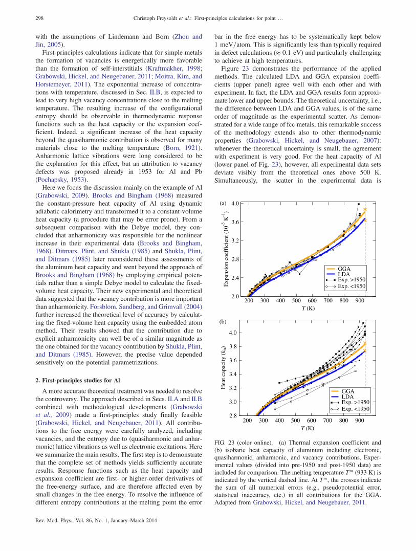
VI. Conclusions and Outlook 299Acknowledgments 300References 300
I. INTRODUCTION
Point defects and impurities often play a decisive role in thephysical properties of materials. Experimental defect identi-fication is typically difficult and indirect, usually requiringan ingenious combination of different techniques. First-principles calculations have emerged as a powerful approachthat complements experiments and has become reliableenough to serve as a predictive tool. This methodology isnow practiced by a large and growing number of researchgroups around the world. Due to the importance of this activefield a number of textbooks and overview articles have beenpublished (Leibfried and Breuer, 1978; Estreicher, 1995,2000; Van de Walle and Neugebauer, 2004; Drabold andEstreicher, 2007; Alkauskas et al., 2011; Evarestov, 2012).Rapid methodological developments over the last few yearsmake this a timely moment to present a comprehensiveoverview of the state of the art and the major achievementsand insights that have been obtained. Our goals are to(1) address the fundamental physics issues that underlie themethods; (2) unify the methodology by covering semicon-ductors, insulators, and metals on the same footing; (3) devoteparticular attention to the impressive methodological progressthat has been achieved within the past few years; and(4) provide a critical assessment of areas in which futureresearch is most needed.A formalism based on formation energies allows calcula-
tion of defect and impurity equilibrium structures and con-centrations. In the case of semiconductors and insulators, italso allows the calculation of the relative stability of thedifferent charge states of a given defect, and hence thethermodynamic and optical transition levels associated withdeep and shallow centers. The formalism is entirely generaland can be applied to any crystalline solid, even though someissues addressed may not be relevant for all material classes.For instance, charged defects and band gaps can occur only innonmetals, i.e., semiconductors, wide-gap materials, andinsulators. From a modeling point of view, the nonmetallicmaterials differ only in the size of the band gap and relatedquantities. For the sake of readability, we will sometimes use“semiconductor” as a synonym for materials with a band gapwhenever the existence of the band gap matters. Section IIprovides an overview of the state-of-the-art methodology forperforming first-principles ground-state calculations fordefects and impurities. Finite-temperature effects, i.e., theevaluation of free energies that include effects beyondconfigurational entropy, will also be comprehensively treated.The electronic ground state provides a variety of additionalresponse properties that are accessible with dedicated experi-ments and theory (see Sec. I.B.4). However, the calculation ofresponse or even dynamical properties (such as local vibra-tional modes, phonon scattering, or localized electronicexcitations) will not be discussed in detail within this reviewdue to space limitations.An area that has proved problematic in the past is related to
the lattice geometry in which the calculations are performed.Typically, one addresses the dilute limit, in which thedefect concentration is low and defect-defect interactionsare negligible. When performing calculations for defectsusing periodic boundary conditions, in the so-called supercell
254 Christoph Freysoldt et al.: First-principles calculations for point …
approach, interactions may affect the calculated formationenergies and transition levels. Electrostatic interactions, whichoccur in the case of charged defects in semiconductors andinsulators, decay particularly slowly with increasing supercellsize. Errors may also arise due to defect wave-functionoverlap, magnetic interactions, and strain. Rigorous trans-formations and extrapolation schemes are therefore critical todescribe the accurate asymptotic limit. All of this is addressedin Sec. III.Density functional theory (DFT), often in conjunction with
pseudopotentials or projector augmented wave potentials, hasemerged as the most commonly used first-principles approachfor defect calculations. When used with the traditional local orsemilocal exchange-correlation (xc) functionals, such as thelocal density approximation (LDA) or generalized gradientapproximation (GGA), this approach has been limited inits ability to predict properties associated with the electronicstructure of materials due to the so-called “band-gapproblem.” Great progress has been made in overcoming thisdeficiency, both by going beyond DFT and by implementingadvanced functionals within DFT. Section IV is devoted tothese issues, including discussion and critical comparison ofapproaches such as the quasiparticle (QP) GW method,DFTþ U, and hybrid functionals.Defect calculations have been pushed forward by the need
for a better theoretical understanding of defects in a widerange of technologies such as electronic and optoelectronicdevices, solar cells, structural materials, and catalysts, just to aname a few. While a comprehensive overview of the insightsgained for these applications is desirable, it would clearlyexceed the limits of our review. Instead, Sec. Vexemplifies themethodology in an applied context by two illustrative casestudies. Section VI, finally, includes a critical outlook on thoseareas that will benefit from additional research.
A. Role of point defects and impurities in solids
1. Doping
Various properties of materials are controlled by thepresence of defects and impurities. An outstanding exampleoccurs in the case of semiconductors, where the incorporationof impurities even in small concentrations determines theelectrical conductivity. The fabrication of p-type and n-typedoped layers underlies the design of virtually all electronicand optoelectronic devices. To achieve such control, compre-hensive knowledge of the fundamental processes that controldoping is required, and first-principles calculations have madeimportant contributions to this knowledge.Shallow dopants (i.e., heterovalent impurities with small
ionization energies that easily release carriers to the host)render the material n-type or p-type conductive. This con-ductivity can be counteracted by the presence of compensatingcenters in the form of either native point defects or impurities.These centers can also introduce deep levels that affectrecombination rates and cause optical absorption or lumines-cence. Even in well-established semiconductors such as Si orGe, achieving high and well-controlled doping levels is still anactive area of research (Voyles et al., 2002). Some othersemiconductors have very attractive intrinsic properties, but
have not been amenable to device applications because ofa lack of control over their conductivity. These problems tendto be particularly severe in the case of wide-band-gapsemiconductors.Several studies have attempted to identify the underlying
reasons for these difficulties (Zhang, Wei, and Zunger, 1999;Walukiewicz, 2001). A general conclusion that can be drawnfrom such investigations is that n-type doping is difficult whenthe energy of the conduction-band minimum (CBM) is highon an absolute energy scale (e.g., referenced to the vacuumlevel); and p-type doping is difficult when the energy of thevalence-band maximum (VBM) is low. This notion is actuallyfairly intuitive. For instance, in the case of shallow donors, thegoal is to introduce a filled electronic state with an energylevel higher than the CBM, which results in an electron beingdonated to the conduction band (see Sec. II.D.2). Theremaining positive defect in turn induces a shallow, hydro-genic effective-mass state slightly below the CBM. When theCBM of the semiconductor is high in energy, the range ofimpurities that can accomplish this feat is limited. In addition,any processes that can lead to a lowering of the energy of theadded electron will be particularly favored if the CBM is high;such processes include spontaneous formation of defects andatomic relaxation of the impurity away from its substitu-tional site.While general rules for describing doping in semiconduc-
tors are useful in elucidating the underlying physics, they turnout to be inadequate and potentially misleading when appliedto specific cases. For instance, such rules typically predict thatit is not possible to dope GaN p type. In reality, acceptordoping of GaN is difficult but by no means impossible: room-temperature hole concentrations on the order of 1018 cm−3 arenow routinely achieved. One has to conclude that there is nosubstitute for considering every case individually. This is aformidable task experimentally, but first-principles calcula-tions are now capable of providing detailed understanding andpredictions.
2. Overcoming doping limits and achieving ambipolar doping
In some semiconductors, doping is in principle straightfor-ward, but achieving the increasingly higher doping levels thatare required for novel devices can be challenging. At highdoping levels, self-compensation sets in, i.e., not every dopantthat is incorporated yields a carrier. In many cases, compen-sation can be attributed to the formation of point defects.Native point defects have also often been invoked to explain
unintentional conductivity in semiconductors and insulators.There has been a long-standing belief that native defects suchas vacancies or self-interstitials can act as a source of doping,particularly in wide-band-gap semiconductors. This belief isbased largely on “circumstantial evidence,” such as trendsobserved when growing or annealing in environments that arerich or poor in one particular constituent. Direct experimentalverification (or refutation) has been lacking, however, mainlydue to the difficulty in establishing quantitative measurementsrelating to the presence of point defects. ZnO is a primeexample of a wide-band-gap oxide in which these issues havelong been debated. First-principles calculations can provide
Christoph Freysoldt et al.: First-principles calculations for point … 255
powerful insights, and ZnO will be the subject of one of thecase studies presented in Sec. V.Bringing unintentional doping under control is a first and
essential step for achieving ambipolar doping. Galliumnitride, a semiconductor that is now the basis of the rapidlygrowing solid-state lighting industry, offers a striking exam-ple. Until about 1990, all GaN material that was grown wasinvariably n type, and almost all reports attributed this to pointdefects (in particular, nitrogen vacancies). It gradually becameclear, however, partly thanks to first-principles calculations,that the conductivity was actually due to unintentionallyincorporated impurities. Improved high-purity growth tech-niques brought these contamination problems under controland opened the path for achieving p-type doping. Morerecently, ZnO followed a similar trajectory, although in thatcase achieving p-type doping is still a major problem, asdiscussed in Sec. V.A.2.The following factors need to be considered when discus-
sing doping of semiconductors and its limitations:
a. Solubility
A high free-carrier concentration requires a high concen-tration of the dopant impurity. The solubility corresponds tothe maximum concentration that the impurity can attain in thesemiconductor, under conditions of thermodynamic equilib-rium. This concentration depends on temperature and on theabundance of the impurity as well as the host constituents inthe growth environment, as determined by chemical potentials(see Sec. II.B.2).
b. Ionization energy
For a shallow donor or acceptor, the ionization energydetermines the fraction of dopants that will be ionized andhence contribute free carriers at a given temperature. A highionization energy limits the doping efficiency. Ionizationenergies of shallow dopants are predominantly determinedby intrinsic properties of the semiconductor, such as theeffective masses and dielectric constant.
c. Incorporation of impurities in other configurations
Most dopant impurities must reside on substitutional sitesin order to exhibit the desired electrical activity. For instance,in order for Mg in GaN to act as an acceptor, it needs to beincorporated on the gallium site. If Mg is incorporated in aninterstitial position, it actually acts as a donor and hencecauses compensation. Another instance of impurities incor-porating in undesirable configurations consists of the so-calledDX centers. The prototype DX center is Si in AlGaAs(Mooney, 1992). In GaAs and in AlGaAs with low Al content,Si resides on the cation site and behaves as a shallow donor,but when the Al content exceeds a critical value, Si behaves asa deep acceptor. This has been attributed to Si being displacedfrom the substitutional site toward an interstitial position(Chadi and Chang, 1988).
d. Compensation by native point defects
Native defects are point defects intrinsic to the semi-conductor, such as vacancies (missing atoms), self-interstitials
(additional atoms incorporated on sites other than substitu-tional sites), and antisites (in a compound semiconductor, acation on a nominal anion site, or vice versa). Native pointdefects usually counteract the prevailing conductivity of thesemiconductors, acting as compensation centers.
e. Compensation by foreign impurities
In spite of experimental attempts to maintain high purity,unintentional incorporation of impurities that are present inthe growth environment is unavoidable. Obviously, whendoping with acceptors in order to obtain p-type conductivity,incorporation of impurities that act as donors should becarefully controlled. Such control may be more difficult thanis obvious at first sight. The chemical potential of theunintentional impurity is largely independent of the intendeddoping type, causing its formation energy to be determined bythe position of the Fermi level (see Sec. I.B.1). A contami-nating impurity with donor character will thus be incorporatedin much larger concentrations in p-type material than inn-type material.Each and every one of the factors listed here can be explicitly
examined using the computational approach described inSecs. I.B and II, as illustrated for ZnO in Sec. V.A.
3. Diffusion
Diffusion is a problem of great importance in solids. In thecontext of doping, diffusion will determine the doping profile.Dopants incorporated during growth may diffuse inside thegrowing material at the high temperatures used for high-quality growth. Alternatively, doping can be achieved bydirect diffusion of impurities from a solid or gaseous source.Finally, implantation can be used, but this usually requires asubsequent annealing step during which diffusion of impu-rities determines their final location in the lattice. Diffusioncan also play a role in device degradation.The issue of doping clearly shows that diffusion is of high
significance for semiconductors, but it is equally importantfor structural metals [e.g., hydrogen diffusion causing embrit-tlement (Du et al., 2011)], ceramics [e.g., impurity diffusion inthermal barrier coatings (Milas, Hinnemann, and Carter,2011)], or in the dehydrogenation of hydrogen storagematerials (Peles and Van de Walle, 2007).Diffusion of impurities is usually assisted by point defects
in both metals (Adda and Philibert, 1966; Seeger et al., 1970)and semiconductors (Fahey, Griffin, and Plummer, 1989;Nichols, Van de Walle, and Pantelides, 1989). A substitutionalimpurity only rarely diffuses by a direct exchange mechanism,where it exchanges places with a neighboring atom (Pandey,1986; Windl, 2006; Janotti and Van de Walle, 2007a). It ismuch more common for diffusion to proceed via a vacancymechanism, in which the impurity jumps into a vacancy on aneighboring site, or an interstitial mechanism, in which, forinstance, a self-interstitial kicks the impurity out of a substitu-tional site and the impurity then migrates through an inter-stitial channel. As a general trend, interstitials move morereadily than vacancies, but are less abundant in equilibriumdue to their higher formation energies. All of this highlightsthe importance of building a thorough understanding of theformation and migration of native point defects.
256 Christoph Freysoldt et al.: First-principles calculations for point …
Diffusion also plays a crucial role in structural materials.For instance, the diffusion of alloying elements in thelow-percentage regime governs the kinetics of segregationand phase transformations. Point defects also tend to pindislocations or even grain boundaries, which play a crucialrole in plasticity. The motion of the dislocation is then directlylinked to the diffusion of the pinning point defect.Actual barriers for hopping processes can be obtained from
first-principles calculations. The nudged elastic band method(Henkelman, Uberuaga, and Jónsson, 2000) has provenparticularly useful for automating the search for a saddlepoint. Migration of defects or impurities can also be studieddirectly via molecular dynamics (Estreicher, Fedders, andOrdejon, 2001) or through the calculation of total-energysurfaces. Such surfaces provide direct insight into stableconfigurations and migration paths, and they show the locationof saddle points, providing values for migration barriers(Van de Walle et al., 1989). They allow for the calculationof finite-temperature diffusion coefficients (Blöchl, Van deWalle, and Pantelides, 1990), and they are also useful foridentifying spatial locations where additional local minima(metastable configurations) might occur. A guide to theconstruction of total-energy surfaces can be found inSec. II.G of Van de Walle and Neugebauer (2004).
4. Thermodynamics and phase stability
In general, defect formation energies are assumed to belargely independent of temperature. The configurationalentropy usually dominates (see Sec. II.A.1) and determinesthe temperature dependence of the defect concentration inthermodynamic equilibrium. Additional entropy contributionsthat could result in temperature-dependent defect formationenergies include (1) vibrational (phonon) contributions (thecreation of a defect modifies the chemical bonds and thus thebond strength in its vicinity), (2) electronic contributions(which are commonly small for semiconductors but can besizable for metals), and (3) magnetic excitations.These entropy contributions to the formation energy have
been commonly neglected, for a number of reasons. First, forcommon defect concentrations that are well below 10−4,configurational entropy per defect is larger than 10kB andis therefore by far the most dominant entropy contribution.Second, computing vibrational and magnetic entropyincreases the computational effort by several orders ofmagnitude compared to a static (T ¼ 0 K) defect calculation.We note that, because of the high cost of computing thedefect-induced changes in the phonon spectra, elastic modelsthat consider only the change of elasticity around the defect(i.e., the long-wavelength part of the phonon spectra) havebeen proposed (Mishin, Sorensen, and Voter, 2001). Third, forsemiconductors and insulators the largest uncertainty inpredicting accurate defect formation energies has been thenotorious band-gap problem of semilocal DFT xc functionals,resulting in errors of several tenths of an electron volt.Compared to this error the missing entropy contributionswere regarded as small. However, with the advent of newtheoretical techniques (see Sec. IV) the predictive power hasgreatly increased, making the inclusion of entropy contribu-tions essential. In the case of metals the spurious
self-interaction that is behind the band-gap problem is largelyabsent due to efficient screening. Since in metals the equi-librium defect concentrations can be experimentally accessedwith high precision and over a large temperature range, theinclusion of all entropy effects is essential for an accuratedescription of defects, as shown in Sec. II.B.3.While the impact of point defects on electronic properties is
well known, their impact on thermodynamic bulk properties(such as heat capacity, thermal expansion, etc.) that are closelyrelated to bulk phase stability has often been assumed to benegligible. As shown in Sec. V.B point defects can have asignificant impact on such properties at temperatures close tomelting.
B. Key quantities
In this review, we focus on calculations of defects in asupercell geometry. (From now on, we use the term “defect” togenerically refer to both point defects and impurities.) Thedefect is surrounded by a finite number of atoms, and thiswhole structure is periodically repeated (Messmer andWatkins, 1972; Louie, Schlüter, and Chelikowsky, 1976).Provided the defects are sufficiently well separated, propertiesof a single isolated defect can be derived. While alternatives tothe supercell approach exist [see, e.g., Deák (2000) andPacchioni (2000)], employing supercells has the followingadvantages: (1) It allows the use of mathematical techniquesthat require translational periodicity of the system. (2) Theband structure of the host crystal is well described. Thiscontrasts with cluster approaches, where the host is modeledby a finite number of atoms terminated at a surface, which istypically hydrogenated in order to eliminate surface states inthe case of semiconductors or embedded in point charges orpseudopotentials in the case of insulators (Pacchioni, 2000).Even fairly large clusters still produce sizable quantumconfinement effects that significantly affect the band structure,and interactions between defect wave functions and the clustersurface are hard to avoid. (3) The results are straightforward tointerpret, unlike, for instance, the Green’s function approach(Car et al., 1984), which is challenging from a programmingpoint of view, and less transparent than the supercell techniquefrom a physics standpoint. Supercells are discussed in detail inSec. III.
1. Formation energies
The formation energy of a defect X in charge state q isdefined as (Zhang and Northrup, 1991; Van de Walle et al.,1993)
Ef½Xq� ¼ Etot½Xq� − Etot½bulk� −Xi
niμi þ qEF þ Ecorr: (1)
Etot½Xq� is the total energy derived from a supercell calculationcontaining the defect X, and Etot½bulk� is the total energy forthe perfect crystal using an equivalent supercell. The integer niindicates the number of atoms of type i (host atoms orimpurity atoms) that have been added to (ni > 0) or removedfrom (ni < 0) the supercell to form the defect, and the μi arethe corresponding chemical potentials of these species.Chemical potentials represent the energy of the reservoirs
Christoph Freysoldt et al.: First-principles calculations for point … 257
with which atoms are being exchanged; they are discussed indetail in Sec. II.B.2. The analog of the chemical potential for“charge” is given by the chemical potential of the electrons,i.e., the Fermi energyEF. Ecorr, finally, is a correction term thataccounts for finite k-point sampling in the case of shallowimpurities, or for elastic and/or electrostatic interactionsbetween supercells. These issues are explored in detail inSec. III.Thermodynamic considerations relating to free energies
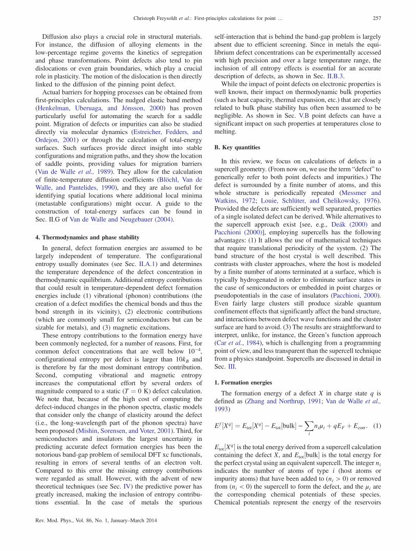
and entropies are discussed in Secs. II.A and II.B. A schematicdiagram of the defect formation energy as a function of theFermi-level position and for various charge states q is shownin Fig. 1.We indicate the charge state of a defect with a superscript q:
for a neutral defect, q ¼ 0; if one electron is removed,q ¼ þ1; if one electron is added, q ¼ −1, etc. This isequivalent to the historical Kröger-Vink notation (Kröger,1974), in which neutral charge states (0) are indicated bya × superscript, negative charge states by a 0, and positivecharge states by a •. In a metal, only neutral defects can occur.In a semiconductor or insulator, the defect can typicallyassume various charge states, accomplished through exchang-ing electrons with an electron reservoir, the energy of which isthe electron chemical potential, or Fermi level EF, conven-tionally referenced to the VBM in the bulk. An alignmentprocedure is required to relate the potential in the supercell tothat in the bulk material; this is discussed in Sec. III.C.Our approach centers around defining and calculating
formation energies for individual defects and as such it isdistinct from the Kröger-Vink approach (Kröger, 1974), inwhich the physics of defects is expressed in terms ofexplicit reactions that involve pairs of defects, e.g.,Frenkel pairs. In a more formal notation our approachcorresponds to a grand canonical approach where defect-defect interaction takes place only via interaction with theelectron reservoir (defined by the chemical potential of the
electrons EF). Since the total system containing all thedefects has a fixed number of electrons and must be chargeneutral, the grand canonical description has to be mappedback onto a canonical one. This is done by identifyingin a self-consistent manner the position of the electronreservoir for which the system becomes charge neutral (seeSec. II.B.2). In contrast, the Kröger-Vink approach (Kröger,1974) constructs reactions (creation of pairs or multiples ofdefects) that keep the system charge neutral. For realisticsystems the number of reactions can become significantlylarger than the number of defects and their charge states,making careful bookkeeping challenging. In contrast, thegrand canonical approach using individual defect energies asa function of the energy of the electron reservoir requires noad hoc assumptions about which reactions are important butincludes all of them in an intuitive and transparent manner.The approach provides a direct way to determine the defectconcentrations and Fermi-level position in the material as afunction of growth or annealing conditions (see Secs. II.B.2and II.B.3).
2. Complex formation and binding energies
At higher concentrations or at low temperatures defects notonly occur as isolated centers but can also form defectcomplexes. Hydrogen complexes are a prime example. Dueto the small size of the H atom and its high chemical reactivityhydrogen easily forms complexes with other impurities orwith native point defects. Among the latter, complexes withvacancies are particularly stable since the inner surface of avacancy provides highly stable binding sites for one or more Hatoms. Defect reactions that result in complex formation are ofhigh technological relevance for both semiconductors andmetals.In semiconductors, complexes are often detrimental to
device performance since the electronic behavior of thecomplex is typically qualitatively different from that of itsconstituents. For example, Mg in GaN is a shallow acceptorwhich renders the material p-type conductive. Complexingwith H removes the acceptor state and results in a neutralcomplex: the Mg in the complex no longer acts as an acceptor(Neugebauer and Van de Walle, 1996; Lyons, Janotti, and Vande Walle, 2012). This mechanism by which the formation of acomplex destroys the doping character of an impurity is calledpassivation. Complex formation in semiconductors is oftendriven by the strong attractive electrostatic interactionbetween defects with opposite charge states. This explainsthe often compensating nature of defects since donor(acceptor) dopants attract point defects or impurities thatbehave as acceptors (donors), resulting in a charge-neutral andelectrically inactive complex.In metals, where Coulomb interaction between defects is
negligible due to efficient screening, defects are neverthelessknown to form centers consisting of two or more defects orimpurities. The driving forces here are local elastic inter-actions and the formation of covalent bonds. For example, H isknown to form stable complexes with vacancies. At suffi-ciently high concentrations the formation energy of thevacancy-hydrogen complex becomes lower than that ofthe vacancy resulting in concentrations that are orders
FIG. 1 (color online). Schematic illustration of formation energyEf vs Fermi level EF for an amphoteric defect that can occur inthree charge states q:þ1, 0, and −1. Solid lines correspond to theformation energy as defined by Eq. (1). The defect exhibits twocharge-state transition levels (see Sec. II.D): a deep donor levelεðþ=0Þ and a deep acceptor level εð0=−Þ. The thick solid linesindicate the energetically most favorable charge state for a givenFermi level.
258 Christoph Freysoldt et al.: First-principles calculations for point …
of magnitude larger than the concentration of barevacancies (superabundant vacancies) (Nazarov, Hickel, andNeugebauer, 2012).An advantage of the grand canonical formulation is that the
formation energy of a complex (which determines its con-centration) is defined in the same way as for isolated defects,i.e., by Eq. (1). Another key quantity for complexes is theirbinding energy, i.e., the energy difference between thecomplex formation energy and the sum of the formationenergies of its isolated constituents. For example, for acomplex consisting of two defects A and B the complexbinding energy is
Eb ¼ Ef½A� þ Ef½B� − Ef½AB�: (2)
A positive binding energy implies that the energy to createisolated defects is higher than that for forming a complex,i.e., the interaction between defects A and B is attractive andcomplex formation becomes thermodynamically advanta-geous. However, a positive binding energy indicates onlythat complexes can in principle be formed, but not that theywill occur in sizable concentrations. The reason is the verydifferent configurational entropy of a pair of isolated defectsversus that of a complex. For a more detailed discussion, seeSec. II.F in Van de Walle and Neugebauer (2004). It shouldalso be noted that complex formation does not change thenumber and nature of participating species. Thus, thecomplex binding energy is independent of the chemicalpotentials.
3. Charge-state transition levels in semiconductors and insulators
Defects in semiconductors and insulators almost alwaysintroduce levels in the band gap or near the band edges. Theselevels determine the electronic behavior, and they are alsooften used as the basis for experimental detection or identi-fication of the defect. Accurate calculation of these levels istherefore essential for defect identification and characteriza-tion. In principle, internal excitations of the defect can occur inwhich the charge state of the defect remains unchanged. Morecommonly, however, carriers are exchanged with the semi-conductor host and a transition to a different charge stateoccurs. These different charge states may correspond to quitedifferent local lattice configurations. It is important to realizethat the Kohn-Sham (KS) levels that result from a band-structure calculation for the center cannot directly be identi-fied with any levels that are relevant for experiment, even ifthere were no concerns about the accuracy of the KS band gap.Instead, the total energies of the defect configurations beforeand after the transition must be considered.The thermodynamic transition level εðq1=q2Þ is defined as
the Fermi-level position for which the formation energies ofcharge states q1 and q2 are equal:
εðq1=q2Þ ¼EfðXq1 ;EF ¼ 0Þ − EfðXq2 ;EF ¼ 0Þ
q2 − q1; (3)
where EfðXq;EF ¼ 0Þ is the formation energy of the defect Xin the charge state q when the Fermi level is at the VBM(EF ¼ 0). The experimental significance of this level is that
for Fermi-level positions below εðq1=q2Þ, charge state q1 isstable, while for Fermi-level positions above εðq1=q2Þ, chargestate q2 is stable. This concept is illustrated in Fig. 1 for asystem with three charge states and two transition levels.Thermodynamic transition levels can be observed in experi-
ments where the final charge state can fully relax to itsequilibrium configuration after the transition, such as in deep-level transient spectroscopy (DLTS) (Lannoo and Bourgoin,1981, 1983; Mooney, 1999). Transition levels correspond tothermal ionization energies. Conventionally, if a transitionlevel is positioned such that the defect is likely to be thermallyionized at room temperature (or at device operating temper-atures), this transition level is called a shallow level; if it isunlikely to be ionized at room temperature, it is called a deeplevel. A detailed discussion of deep versus shallow levels isgiven in Sec. II.D.For purposes of defining the thermal ionization energy, it is
implied that for each charge state the atomic structure isrelaxed to its equilibrium configuration. The atomic positionsin these equilibrium configurations are not necessarily thesame for both charge states. Indeed, it is precisely thisdifference in relaxation that leads to the difference betweenthermodynamic transition levels and optical transition levels,discussed in detail in Sec. II.E.
4. Quantities amenable to comparison with experiment
The ability to compare with experimental results is ofparamount importance. First, such comparisons are essentialfor validation of the computational approach. Second, theability to help interpret and explain experimental observationsis a crucial asset of the first-principles calculations. Theultimate goal is to reliably predict structures and propertiesthat can be experimentally implemented and observed. Wealso note that experimental observations of defects in solidshave their own limitations, which computational studies canaid in overcoming. Here we touch upon some of the keyquantities that can be obtained from first-principles calcula-tions, and how they are linked to experimental techniques; anexcellent overview of such techniques is provided byMcCluskey and Haller (2012).
a. Defect concentrations
The formation energy defined in Eq. (1) can be usedto calculate concentrations, as discussed in Sec. II.B.Concentrations of impurities can be experimentally deter-mined using secondary ion mass spectrometry (SIMS) orRutherford backscattering spectrometry. Determining theconcentration of native point defects is more difficult; electronparamagnetic resonance (EPR) is one of the few techniquesthat can both identify the nature of a defect and accuratelydetermine its concentration. EPR is discussed in more detailbelow. Positron annihilation spectroscopy (PAS) (Puska andNieminen, 1994) can also identify and measure point defects,but is typically limited to detection of vacancies. A commonlyused method in metals is dilatometry in combinationwith precision measurements of the lattice constant(Simmons and Balluffi, 1960). Knowing both the change inthe lattice constant and the macroscopic (dilatometric) changeallows separating the effect of thermal expansion from that of
Christoph Freysoldt et al.: First-principles calculations for point … 259
vacancy creation. Less frequently used are electrical-resistivity (Cotterill et al., 1965) and specific-heat measure-ments (Kraftmakher, 1998). Resistivity measurements probefor the additional scattering due to defects. The specific heatassociated with the creation of intrinsic defects (notablyvacancies) can be separated from bulk contributions via itsexponential increase with rising temperature or the character-istic time scale of defect formation. Another approachmeasures electrical noise and uses sophisticated theoreticaltools to extract dynamical defect properties such as creationand annihilation rates or equilibrium concentrations (Celasco,Fiorillo, and Mazzetti, 1976).
b. Atomic structure
Direct measurements of atomic structure and bond lengthsaround an impurity can be obtained from extended x-rayabsorption fine structure (EXAFS) (Lee et al., 1981) but onlyin the case of impurities with relatively heavy mass.
c. Scanning tunneling microscopy and spectroscopy
Scanning tunneling microscopy (STM) and its variable-biasvariant, scanning tunneling spectroscopy (STS), are powerfultools for revealing the atomic and electronic structure ofsurfaces. As such, STM and STS can also detect defects on orslightly below surfaces. Insight into bulklike defects can beobtained from cross-sectional STM after cleavage, providedthat the investigated cleavage surface is atomically flat,exhibits no states within the bulk band gap, and has a lowdensity of STM-observable surface defects (Feenstra, 1994;Garleff, Wijnheijmer, and Koenraad, 2011). Prominent exam-ples are the GaAs (110) surface under ultrahigh-vacuumconditions (Feenstra, 1994; Tsuruoka et al., 2002;Mikkelsen and Lundgren, 2005; Garleff, Wijnheijmer, andKoenraad, 2011) or passivated Si surfaces (Garleff,Wijnheijmer, and Koenraad, 2011). The simulation of STMimages theoretically is well established (Tersoff and Hamann,1985). The relation of STS data to properties of the bulkdefect, however, requires a careful analysis (Grandidier et al.,2000; Garleff, Wijnheijmer, and Koenraad, 2011).
d. g factors and hyperfine parameters
EPR is one of the most powerful techniques for the studyand identification of defects in semiconductors and insulators(Watkins, 1999). Experimental EPR data provide informationabout the chemical identity of the atoms in the vicinity of thedefect as well as about the symmetry. The ability to directlycompare with calculated values for specific defect configu-rations then allows an explicit identification of the micro-scopic structure (Van de Walle, 1990; Van de Walle andBlöchl, 1993; Ricci et al., 2003).EPR relies on the presence of unpaired electrons. In cases
where the stable ground-state configuration of the defect is notparamagnetic, optical excitation can often be used to generate ametastable charge statewith a net spin density.Optically detectedmagnetic resonance (ODMR) is a variant of the technique thatcan offer additional information about the defect-induced levelsin the band gap (Kennedy and Glaser, 1999).
EPR spectra yield two types of information, namely,hyperfine parameters and g tensors. Hyperfine parameterscan be calculated directly from the ground-state spin density,but all-electron wave functions are required. In a pseudopo-tential approach these can be obtained by combining free-atom wave functions with the pseudo-wave-functionsobtained in the defect calculation (Van de Walle andBlöchl, 1993). In the projector augmented wave (PAW)method, this information can be extracted directly from theall-electron spin density (Blöchl, 2000).Computing g tensors posed additional complexities, par-
ticularly the implementation of a gauge-invariant theorywithin a pseudopotential or PAW approach (Pickard andMauri, 2001); this problem was successfully addressed byPickard and Mauri (2002).
e. NMR chemical shifts
Nuclear magnetic resonance (NMR) is used for moleculesas well as solids to provide chemical and structural informa-tion. The technique has been employed, e.g., to study pointdefects in irradiated aluminum and copper (Minier, Andreani,and Minier, 1978). When combined with first-principlescalculations of chemical shifts, the approach allows anunambiguous determination of the microscopic structure.The computation of these shifts required developments similarto those mentioned for g tensors above (Pickard andMauri, 2001).
f. Mössbauer spectroscopy
Similarly to NMR, Mössbauer spectroscopy probeschanges in the nuclear energy levels and allows detectionof interactions of point defects with neighboring atoms(Czjzek and Berger, 1970).
g. Vibrational frequencies
Defects often give rise to local vibrational modes (LVMs),whose frequencies and polarization contain information aboutthe chemical nature of the atoms involved in the bond as wellas the bonding environment (McCluskey, 2000). Light impu-rities, in particular, exhibit distinct LVMs that are often wellabove the bulk phonon spectrum. A direct comparison ofsignals obtained with Raman spectroscopy or Fourier-transform infrared spectroscopy with first-principles calcula-tions can greatly aid in identifying the nature and localstructure of the defect.Vibrational frequencies can be directly extracted from
the velocity-velocity autocorrelation function of moleculardynamics runs (Estreicher, 2000; Estreicher et al., 2009).Alternatively, vibrational frequencies corresponding to astretching or wagging mode of a particular bond can beextracted from a dynamical matrix based on calculated forces.In the case of light impurities, anharmonic corrections can besizable. These can be evaluated by focusing on the motion ofthe light impurity only, keeping all other atoms fixed, andmapping out the potential energy as a function of displace-ment (Van de Walle, 1998a; Limpijumnong, Northrup, andVan de Walle, 2003).
260 Christoph Freysoldt et al.: First-principles calculations for point …
Charge-state transition levels were introduced in Sec. I.B.3and will be discussed in more detail in Secs. II.D and II.E.Thermodynamic transition levels can be derived from experi-ments such as DLTS (Lannoo and Bourgoin, 1981, 1983;Mooney, 1999) or temperature-dependent Hall measurements(Look, 1992), while optical levels can be observed in photo-luminescence, absorption, or cathodoluminescence experi-ments (Davies, 1999). The identification of the underlyingdefect is greatly helped by comparison to theory, notably incomplex cases (Hourahine et al., 2000).
C. Requirements for theoretical and computational treatments
1. Electronic-structure approaches
Various methods are in principle available to investigatethe electronic structure of solids in general and defects inparticular.Tight-binding methods use a local basis set, for which the
Hamiltonian matrix elements decrease rapidly with increasingdistance between the orbitals. Thus, instead of having todiagonalize the full Hamiltonian matrix, most of the matrixelements vanish and only a sparsematrix has to be diagonalized.Twomainapproaches aredistinguished, basedonhow thematrixelements are determined. Within the empirical tight-bindingapproach, matrix elements are usually fitted to experiment, andthe lack of a consistent prescription is a problem. First-principlestight-binding methods, on the other hand, use local orbitals toexplicitly calculate the matrix elements. The choice of orbitalsis critical: instead of the standard atomic orbitals, specificallydesigned highly localized orbitals (e.g., Gaussians) are used.Approximations are made in neglecting some of the multicenterintegrals and charge self-consistency. The description can beimproved by using a point-charge model to take charge transferand polarizability into account (Elstner et al., 1998).The Hartree-Fock (HF) method is described in detail in
Sec. IV.A. For defect calculations this approach has beenemployed only in a few cases since it is computationally muchmore expensive than density functional theory discussedbelow and provides no advantages with respect to predictivepower. For cluster models, correlated quantum-chemical post-Hartree-Fock methods such as configuration interaction (CI),complete active space methods [complete active space self-consistent field (CASSCF) and complete active space second-order perturbation theory (CASPT2)], or coupled-cluster (CC)methods promise unrivaled theoretical accuracy. However, theenormous computational effort and unfavorable scalingbehavior with respect to system size restrict such methodsto a few tens of atoms. While these approaches can be used forbenchmarking or to answer specific questions, in general theartifacts due to inadequate cluster size may easily undo theadvantages gained from the high level of theory. In contrast,hybrid approaches that are based on a combination of Hartree-Fock theory and DFT have become feasible and highlypopular for defect calculations. The underlying conceptsand the performance of hybrid functionals are discussedin Sec. IV.DFT calculations have become the standard tool for first-
principles calculations of solids. DFT (Hohenberg and Kohn,
1964; Kohn and Sham, 1965) allows a description of themany-body electronic ground state in terms of single-particleequations and an effective potential. The latter consists of theionic potential due to the atomic cores, the Hartree potentialdescribing the electrostatic electron-electron interaction, andthe xc potential that takes into account the many-body effects.This approach has proven to describe with high accuracy suchquantities as atomic geometries and charge densities.Choices have to be made for the basis set and for the xc
functional. The LDA and GGA are still the most widely usedfunctionalswithinDFT,and inmost cases theyproduceaccurateand reliable structural information. It is well recognized,however, that these functionals fail to produce the correct bandstructure; in particular, the band gap of semiconductors andinsulators is severely underestimated (Perdew and Levy, 1983;Sham and Schlüter, 1983). This also affects the position ofdefect-induced states in the band gap, and when these states areoccupied with electrons, the formation energy can also beaffected.AsmentionedwhendiscussingHartree-Fockmethods,great progress has recently been made in overcoming theselimitations, and this is the subject of Sec. IV.All-electron calculations can be carried out with techniques
such as the full-potential linearized augmented plane-wave(FP-LAPW) method (Singh and Nordstrom, 2000) or atom-centered basis sets [e.g., Gaussian (Frisch et al., 2009),CRYSTAL (Dovesi et al., 2005), DMol3 (Delley, 2000), orFHI-AIMS (Blum et al., 2009)]. In most cases, however, anapproximate treatment of the core electrons suffices, leadingto the pseudopotential approach (Pickett, 1989) or the PAWapproach (Blöchl, 1994; Kresse and Joubert, 1999). Thesetend to be computationally more tractable than all-electronapproaches and hence have been most widely used for thelarge system sizes required for first-principles studies ofdefects. The pseudopotential or PAW approximations to dealwith the core electrons are essential for rendering plane-wavebasis sets efficient, but offer advantages also for pseudoatomicorbital basis sets (Sankey and Jansen, 1988; Estreicher,Fedders, and Ordejon, 2001; Soler et al., 2002) or real-spacegrids (Mortensen, Hansen, and Jacobsen, 2005). Most of theexamples given in this review have been obtained based onplane-wave calculations; however, in principle any well-chosen basis set can be used, and the topics covered in thisreview do not depend on this choice.
2. Constraints on accuracy of computational results
Comparing defect concentrations based on calculated for-mation energies with experiment requires high accuracy.Based on the expressions discussed in Sec. II.B, to limitthe error to less than an order of magnitude at a temperatureof 1000 K requires an accuracy of 0.2 eV. More detailedcomparisons, or lower temperatures, require even higheraccuracy. As noted in Sec. I.A.4, electronic-structure calcu-lations for metals are capable of achieving such accuracy, andthe constraints mainly revolve around the inclusion of entropyeffects (see Sec. II.B.3). For semiconductors and insulators,achieving accuracies even of a few tenths of an electron volthas been challenging, and this has also limited the ability tocompare with experimental results for charge-state transitionlevels, let alone to accurately predict concentrations or defect
Christoph Freysoldt et al.: First-principles calculations for point … 261
levels. The most fundamental constraint on accuracy is due tothe approximations in the xc functionals. As shown in Sec. IV,new theoretical techniques allowed great progress in reducingthese uncertainties.Even if approximations in the underlying electronic-struc-
ture methods constitute a hard bound on the achievableaccuracy, guaranteeing this accuracy is often a challengingtask in practical defect calculations. The reason is the largenumber of parameters involved in performing electronic-structure calculations of defects, including the size of thesupercell, completeness of the basis set, and sampling of theBrillouin zone, to name only a few. Even though all theseparameters are controllable, in the sense that they can besystematically improved until convergence is reached, inpractice limitations in the computational resources placesevere restrictions on the extent to which such convergencecan be achieved.Consider, for example, the issue of supercell-size conver-
gence. As discussed in Sec. III.C the electrostatic interactionbetween a charged defect and its periodic images scales as1=L, with L the dimension of the supercell. Thus, in a bruteforce approach, to decrease the error by a factor of 2, thenecessary 3D volume and thus the number of atoms needs toincrease by a factor of 8. Since most DFT implementationsasymptotically scale with the third power of the number ofatoms, the computational effort needed to reduce the error by afactor of 2 requires an increase by a factor of 83 ¼ 512 incomputer time. Improving the accuracy by an order ofmagnitude requires increasing the computation time by afactor of 109. It is therefore of extreme importance to designand employ schemes that improve convergence (see, e.g.,Sec. III.C).Besides supercell-size convergence, an efficient k-point
sampling of the Brillouin zone is also critical. Brillouin-zoneintegration is carried out by replacing the continuous integralby a set of special points. Ideally, such sets contain a minimumnumber of points (to reduce computational effort), conservethe symmetry of the system, and provide an accurate estimateof the integrated quantity. In practice, such sets are generatedwith the Monkhorst-Pack scheme (Monkhorst and Pack,1976), i.e., a regularly spaced mesh of n × n × n points inthe reciprocal-space unit cell. To avoid the inclusion ofextrema (i.e., local maxima or minima) in the band structure,high-symmetry points such as the Γ point should be avoided.Consequently, odd values of n are used for which byconstruction the Γ point is excluded. Most defect geometriesconserve part of the point-group symmetry of the bulk system,and the full set of points in the Brillouin zone can be reducedto a set of points in the irreducible part of the zone. Therequired size of n depends on the material and the consideredphysical quantity. In general, metals require substantiallylarger k-point sets than semiconductors and a careful choiceof the smearing scheme. Furthermore, the consideration ofvibrational contributions to the free energy of the defect callsfor a particularly careful k-point convergence (Grabowski,Hickel, and Neugebauer, 2007).Defects in semiconductors or insulators that exhibit a defect
state in the band gap show an artificial dispersion of thedefect-induced level in the supercell approach. A truly isolateddefect (corresponding to the limit of an infinitely large
supercell) leads to a flat, dispersionless defect level in thethen infinitely small Brillouin zone. Thus, the magnitude ofdispersion is a direct measure of the artificial interactionbetween the defect and its neighboring images. For finite-sized supercells, minima and maxima in the defect bandcorrespond to artificial bonding and antibonding states,respectively. Using special points provides a way of averagingover the defect band and corresponds to extracting non-bonding states that closely resemble the isolated defect inan infinite cell. These considerations imply that the Γ point,which is sometimes used as the single k point for Brillouin-zone integrations because of the numerical simplicity, pro-vides a poor description since defect-defect interactions arestrongest at this point. Further discussions of this issue, as wellas guidelines for dealing with partially occupied defect levels,are included in Sec. III.B.
II. THERMODYNAMIC CONCEPTS
The fundamental methodological approach to calculatingdefect formation energies has been outlined in Sec. I.B.1.As expressed in Eq. (1), defect formation energies aredefined as an energy difference between supercell calcu-lations with and without a defect. Electronic-structurecalculations provide a great deal of additional informationbeyond the formation energy of the defect. An analysis ofthe energy as a function of atomic positions (potentialenergy surface) and defect-state occupations allowsextracting many defect properties, notably the completefinite-temperature thermodynamics. The implementation ofthis concept in first-principles calculations involves a num-ber of technical developments that are discussed in the nextsections. First, however, we review the relevant conceptsfrom statistical mechanics.As noted in Sec. I.A.4, defect formation energies are
generally assumed to be independent of temperature.Nevertheless, even at T ¼ 0 K the proper choice of thechemical potential(s) in Eq. (1) decisively depends on phasestabilities of the considered system (cf. Sec. II.B.2). Mostimportantly, all experimental measurements of defect con-centrations (see Sec. I.B.4) are performed at finite temper-atures. While configurational entropy is the dominantcontribution, other entropy contributions can also becomerelevant (in particular, for metals) and will therefore also bediscussed in this section.In semiconductors and insulators, defects can typically
occur in different charge states. The resulting transition levels(see Sec. I.B.3) are classified into thermodynamic or opticallevels, depending on the time scale of the transition. Eventhough the optical levels are not thermodynamic properties,they can be determined directly from the potential energysurface and will therefore be discussed here. The physicalconcepts related to this distinction will be addressed inSecs. II.D and II.E.
A. Entropy of defects
1. Configurational entropy
Defect formation energies are always positive—otherwisethe host crystal would be unstable. It is therefore the
262 Christoph Freysoldt et al.: First-principles calculations for point …
configurational degree of freedom that allows point defects toform in the first place. The configurational part of the entropyhas to counterbalance the energy cost of defect creation. Ageneral and rigorous approach to treat the configurationalentropy of point defects including their mutual interactionrequires methods such as the cluster expansion technique(Sanchez, Ducastelle, and Gratias, 1984) combined withMonte Carlo simulations. As mentioned in Sec. I, this reviewfocuses on isolated defects and ignores defect-defect inter-actions. This assumption is justified due to the typically lowdefect concentrations (dilute limit) in many physically rel-evant cases. Consider, for instance, vacancies in elementalmetals, which are known to be the dominant defects over awide temperature range (Kraftmakher, 1998). Yet, even closeto the melting temperature their concentrations are typically< 10−3, i.e., even under conditions where defect concentra-tions are high the dilute limit applies.If n is the number of point defects of a specific type andN is
the number of lattice sites, then the numberW of distinct ways(≙microstates) to arrange the defects is (Keer, 1993)
W ¼ ðgNÞ!ðgN − nÞ!n! ≈
ðgNÞnn!
: (4)
Here g is a degeneracy factor accounting for the internaldegrees of freedom of the point defect. For instance, g ¼ 1 forsimple monovacancies but g ¼ 6 for a tetrahedral interstitialsite in a bcc structure since there are six such interstitialpositions per lattice site. Likewise g can capture spin degen-eracy if it is not explicitly included in the electronic entropy(see Sec. II.A.2). Further, Eq. (4) uses the fact that atoms andpoint defects of the same kind are indistinguishable. The firstequation takes into account that creation of a defect reducesthe configuration space for the next defect. However, suchconsiderations make the derivations tedious, in particular,when dealing with more than one type of defect. In the dilutelimit (n ≪ N), the second part of Eq. (4) is a well-justifiedapproximation.The configurational entropy is given by (Keer, 1993)
Sconf ¼ kB ln W; (5)
and the corresponding term entering the free energy is−TSconf . Since W ≥ 1 and T is always positive, −TSconf isalways negative, thus favoring defect formation. Note thatgenerally several kinds of defects exist simultaneously. Thisyields a product W ¼ Q
iWi in the number of configurations,and therefore a summation Sconf ¼ kB
Pi ln Wi in the
entropy.The consideration of Eqs. (4) and (5) in the thermodynamic
limit allows the application of the Stirling approximation,resulting in
Sconfðn; NÞ ¼ kB½n − n lnðn=NÞ þ n lnðgÞ�: (6)
It is convenient to transform this into a per atom quantity thatdepends only on the point-defect concentration c ¼ n=N,
SconfðcÞ ¼ kB½c − c lnðcÞ þ c lnðgÞ�: (7)
By including the penalty energy for creating defects,Econf ¼ cEf, with the energy of formation Ef from Eq. (1),we arrive at the configurational free energy:
FconfðcÞ ¼ EconfðcÞ − TSconfðcÞ¼ cEf½Xq� − TkB½c − c lnðcÞ þ c lnðgÞ�: (8)
This equation gives direct access to the equilibrium defectconcentration as outlined in Sec. II.B.3. Before consideringthe equilibrium concentration, however, we need to take intoaccount the fact that in a fully consistent treatment the defectenergy of formation acquires a temperature and volume orpressure dependence and becomes a Gibbs energy of for-mation, i.e., Ef → Gf. The contributions responsible for thisare the electronic and vibrational entropy, which are discussedin the following sections.
2. Electronic entropy
We aim to compute the formation free energy of an isolateddefect in a fully integrated first-principles approach. Thestarting point is the free-energy Born-Oppenheimer approxi-mation (Cao and Berne, 1993), which is a thermodynamicextension of the standard Born-Oppenheimer approximation.The main result of this approximation is that the ionicmovement, i.e., the motion of the point defect, is governedby the electronic free-energy surface FelðfRIg; V; TÞ. Herethe thermodynamic averaging has been done only over a partof the microscopic configuration space (the electronic degreesof freedom), which should formally not be the case for athermodynamic potential. Therefore, the superscript “el” aswell as the indication of the dependence on the microscopicatomic coordinates ðfRIgÞ is important for distinguishingthese quantities from the full free energy F.Thecrucial step thatallowsforaseparation into thephysically
relevant excitation mechanisms is a Taylor expansion ofFelðfRIg; V; TÞ around the equilibrium positions fR0
Ig:
FelðfRIgÞ ¼ Fel0 þ 1
2
Xk;l
ukul
� ∂2Fel
∂Rk∂Rl
�fR0
I gþOðu3Þ: (9)
Here the zeroth-order term is abbreviated asFel0 ðV; TÞ≔FelðfR0
Ig; V; TÞ, k and l run over all nuclei of thesystem and additionally over the three spatial dimensions foreach nucleus, and uk ¼ Rk − R0
k is the displacement out ofequilibrium.Equilibriumpositions refer to the atomic geometrythat is obtained after introducing the point defect into the perfectbulk and relaxing the atoms until the corresponding forcesare zero. Since forces are related to the first-order term in theexpansion, this term vanishes from Eq. (9). The higher-orderterms correspond to vibrational motion and are discussed inSec. II.A.3.The zeroth-order term in Eq. (9) is related to electronic
entropy. If DFT is performed at finite temperatures, as firstintroduced by Mermin (1965), then the electronic free energyis given as
Fel0 ðV; TÞ ¼ EelðfR0
Ig; V; TÞ − TSelðfR0Ig; V; TÞ: (10)
Christoph Freysoldt et al.: First-principles calculations for point … 263
Here the temperature enters via the energy EelðV; TÞ, due tothe T dependence of the occupation of KS energy levels, aswell as via the second term. The latter contains in Sel theelectronic entropy given by an ideal mixing as
SelðfR0Ig; V; TÞ ¼ −kB
Xi
½ð1 − fiÞ ln ð1 − fiÞ þ fi ln fi�;
(11)
where the sum runs over all electronic states with Fermi-Diracoccupation weights fi ¼ fðT; ϵiÞ. Depending on the way spinpolarization is considered, Eq. (11) is sometimes written withan additional factor of 2.For an accurate treatment of temperature dependences it is
often useful to separate the zero-temperature electronic energyEel0 from Fel
0 as
Fel0 ðV; TÞ ¼ Eel
0 ðVÞ þ ~Fel0 ðV; TÞ: (12)
The remainder ~Fel0 describes the temperature dependence of
both terms in Eq. (10). For a continuous density of states at theFermi level it can be shown (Methfessel and Paxton, 1989)that ~Fel
0 varies quadratically with temperature, which leads to(Kresse and Furthmüller, 1996)
~Fel0 ðV; TÞ ¼ −1
2TSel þOðT3Þ: (13)
3. Vibrational entropy
a. Quasiharmonic excitations
The second-order term in Eq. (9) describes quasiharmonicexcitations due to noninteracting but volume-dependent pho-nons. To arrive at an explicit expression for the correspondingfree energy we first define the dynamical matrix D:
Dk;lðV; TÞ≔1ffiffiffiffiffiffiffiffiffiffiffiffi
MkMlp
�∂2FelðfRIg; V; TÞ∂Rk∂Rl
�fR0
I g; (14)
where Mk (Ml) is the atomic mass of atom k (l). Thedynamical matrix D depends not only on the volume V butalso on the temperature T which is a consequence of thetemperature dependence of the electronic free-energy surfaceFel. Note that at this stage T determines electronic excitationsby the Fermi broadening rather than atomic motion. Next thedynamical matrix is diagonalized,
DðV; TÞwi ¼ ω2i ðV; TÞwi; (15)
resulting in eigenvectors wi and phonon frequencies ωi. Theobtained phonon frequencies allow one to determine the vibra-tional internal energy in the quasiharmonic approximation,
Eqh ¼Xi
�1
2þ ni
�ℏωi; (16)
which yields after the application of some statistics and trans-formations the quasiharmonic free energy (Wallace, 1998):
Fqh ¼Xi
�ℏωi
2þ kBT ln
�1 − exp
�− ℏωi
kBT
���: (17)
For periodic systems it is convenient to transform the real-spacedynamical matrix [Eq. (14)] into its reciprocal-space represen-tation. This allows an accurate interpolation of the phononfrequencies, which is critical for integrals or sums over theBrillouinzone, as inEq. (17).For systemsbreaking translationalsymmetry, such as a solid containing a point defect, a Fouriertransformation is not meaningful and the analysis should beperformed in real space.In practice, the supercells in first-principles calculations of
point defects are of limited size (100–1000 atoms). As a resultthe number of phonon modes entering Eq. (17) is limited. Asshown by Grabowski, Hickel, and Neugebauer (2011), aconsistent treatment of the corresponding bulk referencecalculation guarantees converged results. Specifically, thequasiharmonic free energy of the reference perfect bulksystem needs to be calculated on the identical mesh of phononwave vectors as used for the point defect.Studies of the quasiharmonic contribution to the formation
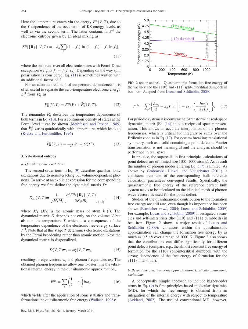
free energy are still rare, even though its importance has beenshown (Estreicher et al., 2004; Lucas and Schäublin, 2009)For example, Lucas and Schäublin (2009) investigated vacan-cies and self-interstitials (the h110i and h111i dumbbells) inbcc iron. Figure 2 shows a major result of Lucas andSchäublin (2009): vibrations within the quasiharmonicapproximation can change the formation free energy by asmuch as 0.5 eV over a range of 1000 K. Figure 2 also showsthat the contributions can differ significantly for differentpoint defects (compare, e.g., the almost constant free energy offormation for the h110i split-interstitial dumbbell with thestrong dependence of the free energy of formation for theh111i interstitial).
b. Beyond the quasiharmonic approximation: Explicitly anharmonicexcitations
A conceptually simple approach to include higher-orderterms in Eq. (9) is first-principles-based molecular dynamics(MD), for which the free energy is obtained from anintegration of the internal energy with respect to temperature(Ackland, 2002). The use of conventional MD, however,
FIG. 2 (color online). Quasiharmonic formation free energy ofthe vacancy and the h110i and h111i split-interstitial dumbbell inbcc iron. Adapted from Lucas and Schäublin, 2009.
264 Christoph Freysoldt et al.: First-principles calculations for point …
requires computation times that are impracticable. Thereforehighly efficient sampling strategies to perform the thermody-namic averages had to be developed (Grabowski et al., 2009).The approaches can be divided into two classes:
(1) Thermodynamic-integration-based techniques, which startfrom a reference system for which the free energy can beeasily obtained either analytically or numerically. Making anadiabatic connection to the true first-principles potentialenergy surface, only the small differences in free energiesbetween reference and full surface need to be sampled.(2) Free-energy perturbation techniques, which use well-approximated phase-space samplings to compute first-orderfree-energy shifts.We focus on the thermodynamic integration method first.
Often the quasiharmonic potential energy surface is a suitablereference system. Note that, while the quasiharmonic calcu-lations discussed above contain quantum effects, the thermo-dynamic integration is commonly performed classically,yielding a classical anharmonic correction Fclas;ah to theclassical free energy Fclas [although extensions are possible(Ramirez et al., 2008)]. Therefore, for a consistent treatmentthe quasiharmonic reference needs to be considered classi-cally, as expressed by Fclas;qh:
Fclas;ah≔Fclas − ðFel0 þ Fclas;qhÞ
¼ ½Fclasλ �λ¼1 − ½Fclas
λ �λ¼0 ¼Z
1
0
dλ
�∂Felλ
∂λ
t;λ: (18)
Here Felλ ðfRIg; tÞ is the λ-dependent electronic free-energy
surface determining the classical motion of the nuclei in thecoupled system and h⋅it;λ denotes the time average at a given λ.Provided the boundary conditions for λ ¼ 0 and λ ¼ 1 arefulfilled, any type of coupled system can be chosen. Inpractice, a simple linear coupling to the quasiharmonicreference,
The use of the thermodynamic integration makes thedetermination of anharmonic entropy contributions a feworders of magnitude more efficient than a conventionalmolecular dynamics simulation. The high accuracies neces-sary to obtain these contributions in the case of point defectsrender the first-principles simulation still a formidable task.
Efforts are therefore under way to explore new methods tofurther reduce computation times. On the one hand, one canreduce the complexity of the first-principles treatment byincorporating analytical assumptions regarding the volumeand temperature dependence of anharmonic contributions(Wu, 1991; Wu and Wentzcovitch, 2009). On the otherhand, the numerical precision can be stepwise improved byapplication of free-energy-perturbation techniques.A strategy combining both approaches is the upsampled
thermodynamic integration using Langevin dynamics(UP-TILD) method (Grabowski et al., 2009). Its main ideais that DFT convergence parameters (for example, the elec-tronic k-point sampling) that provide a low precision can beused to obtain for each thermodynamic integration step aphase-space distribution (termed fRIglowt in the following)which closely resembles the phase-space distribution fRIghightthat would be obtained from parameters yielding highlyconverged results. In this way it is possible to sample variousλ, V, and T values with modest computational resources.However, the resulting free-energy surface h∂Fel
λ =∂λilowt;λ ,which is required as input for the thermodynamic integration,needs to be corrected in a second step. For this purpose free-energy perturbation theory is employed: a small set of NUP
uncorrelated structures fRIglowtu (indexed with tu) is extractedfrom fRIglowt and the upsampling average hΔFeliUPλ iscalculated as
hΔFeliUPλ ¼ 1
NUP
XNUP
u
Fel;lowðfRIglowtu Þ − Fel;lowðfR0IgÞ
− ½Fel;highðfRIglowtu Þ − Fel;highðfR0IgÞ�: (21)
Here Fel;low (Fel;high) refers to the electronic free energycalculated using DFT parameters for low (high) convergence.The λ dependence of hΔFeliupλ is hidden in the trajectoryfRIglowt , which is additionally dependent on the volume andtemperature. In the last step, the quantity of interest, i.e., theconverged h∂Fel
λ =∂λihight;λ , is obtained from
h∂Felλ =∂λihight;λ ¼ h∂Fel
λ =∂λilowt;λ − hΔFeliupλ ;
and thus the anharmonic free energy reads
Fclas;ah ¼Z
1
0
dλh∂Felλ =∂λihight;λ : (22)
The efficiency of this method is exemplified by the fact that inpractice fewer than 100 uncorrelated configurations have to becalculated with high convergence parameters to get statisticalerror bars below 1 meV, whereas a full thermodynamicintegration includes many thousands of configurations(Grabowski et al., 2009).
B. Free energy of formation and defect concentrations
1. Point defects at finite temperatures and pressures
By consistently taking into account the full temperature andvolume dependence of the electronic and vibrational entropy
Christoph Freysoldt et al.: First-principles calculations for point … 265
contributions (see Secs. II.A.2 and II.A.3), the thermody-namically relevant quantity becomes the Gibbs energy offormation Gf. The central formula Eq. (1) changes in such acase to
Gf½Xq�ðP; TÞ ¼ F½Xq�ðΩ0; TÞ − F½bulk�ðΩ; TÞ þ PVf
−Xi
niμiðP; TÞ þ qEF þ Ecorr: (23)
Here F½Xq� is the free energy of a supercell containing thedefect Xq and F½bulk� is the free energy of the correspondingperfect bulk supercell. Both free energies are consistentlycomposed of the contributions discussed in the previoussections:
They are calculated at volumes Ω0 and Ω, respectively, whichcorrespond to the given pressure P. Further, in Eq. (23), Vf isthe volume of formation Vf ¼ Ω0 − Ω, and the chemicalpotentials μi acquire a pressure and temperature dependence.The chemical potentials need to contain the same free-energycontributions as included in F½Xq� and F½bulk�.
2. Chemical potentials
a. Variability and limits
The chemical potentials appearing in the formation (Gibbs)energy, Eqs. (1) and (23), reflect the reservoirs for atoms thatare involved in creating the defect. Chemical potentials of purephases depend on pressure and temperature. To emphasize thestrong dependence of the chemical potential of gases like N2
on temperature and partial pressure, we keep these variables inour notation for μðN2; P; TÞ while omitting them for solidphases for the sake of readability. Ultimately, the experimentalconditions under which the defects are created uniquely definethe relevant reservoirs. Conversely, by varying the chemicalpotentials in the calculation, different experimental scenarioscan be explored. In the general formalism, chemical potentialsare regarded as variables. However, they are subject to specificbounds. These bounds are set by the existence or appearanceof secondary phases. Consider, for instance, growth of acompound semiconductor such as GaN. The chemical poten-tials of Ga and N are linked by the stability of the GaNphase, i.e.,
μGa þ μN ¼ μðGaNÞ: (26)
Bounds on the chemical potentials are set by the formationof metallic Ga and molecular nitrogen, respectively,
μGa ≤ μGaðGametalÞ; (27)
μN ≤ μNðN2; P; TÞ: (28)
When combined with Eq. (26), the lower bounds on μGa andμN transform into upper bounds for the corresponding otherspecies:
μðGaNÞ − μNðN2; P; TÞ ≤ μGa; (29)
μðGaNÞ − μGaðGametalÞ ≤ μN: (30)
When impurities are present, their chemical potentials μi[Eq. (1)] are subject to similar bounds, imposed by theformation of stable phases with the elements of the hostmaterial, or among each other. For instance, when hydrogen ispresent as an impurity in GaN, formation of NH3 may place astricter upper bound on μH than the formation of H2 [depend-ing on the value of μN (Van de Walle and Neugebauer,2003a)]. If two impurities are present, for instance, hydrogenand oxygen, then in addition to the formation of NH3 andGa2O3 the formation of H2O needs to be considered.When direct comparisons with experimental findings are
attempted, one needs to critically assess whether equilibriumconditions apply. For instance, when a material is annealed ata high temperature under an overpressure of a certain element,it may be appropriate to relate the chemical potential of thatspecies with the partial pressure in the gas phase. On the otherhand, the nucleation of solid phases is often kineticallyhindered, which may allow the thermodynamic limits to beexceeded to a certain degree (Abu-Farsakh and Neugebauer,2009). In this context, the concept of constrained thermody-namic equilibrium (Reuter and Scheffler, 2003) can be help-ful, where equilibrium is assumed only between some phases(or defects) in the system, but not all.
b. Chemical potential reference
Numerical values of chemical potentials always dependon their implicit reference. In electronic-structure calculations,chemical potentials can be referenced to the total energyof the elementary phases at T ¼ 0 K. Experimental databasesemploy elementary phases at standard conditions (T ¼ 273.15or 298.15 K and P ¼ 100 or 101.325 kPa). These differentapproaches are equally valid and differ only by the (free)energy of formation of the standard phase in the electronic-structure reference. What is crucial, however, is that aconsistent choice is made for all chemical potentials andformation energies considered.To avoid confusion relating to the choice of reference, it is
advisable to directly include it in the equations by using
first approximation. For the gas phase, the chemical potentialscan be related to partial pressures P by standard thermody-namic expressions. For instance, for N2
2μN ¼ EðN2Þ þ kBT lnPVQ
kBTþ ln
σB0
kBTþ μvib; (35)
where VQ ¼ ð2πℏ2=mkBTÞ3=2 is the quantum volume, B0 isthe rotational constant, and σ is the associated symmetryfactor (2 in the case of homonuclear diatomic molecules). Thevibrational contribution to the chemical potential μvib can bestraightforwardly obtained from the vibrational free energy[Eq. (17)], but should be included only if it is also included forthe bulk phases.
c. Chemical potential of electrons
In semiconductors or insulators, defects commonly appearin charged states. Charge is exchanged with a reservoir ofelectrons, the energy of which is the electron chemicalpotential, in other words, the Fermi energy EF. It shouldbe emphasized that the relevant Fermi energy here is not the(artificial) Fermi energy of the DFT calculations. The latter isadjusted to maintain the total electron number in the defectsupercell calculation when Kohn-Sham states are occupiedaccording to a Fermi-Dirac distribution. The Fermi energy thatis relevant in the real material, in a thermodynamic context,depends on any defects or impurities contained therein and isdetermined by the condition of charge neutrality
XX;q
qcðXqÞ þ nh − ne ¼ 0 (36)
for the combined set of defects Xq, free holes (nh), and freeelectrons (ne). The concentration of the free carriers isformally obtained by an integration of the electronic densityof states DðEÞ,
ne − nh ¼Z
∞
−∞dE
DðEÞ1þ exp½ðE − EFÞ=kBT�
− Nelectron; (37)
where Nelectron is the number of electrons in the neutral bulkcell. In the case of isotropic, parabolic bands with effectivemass m�, and for sufficiently low electron concentrations(nondegenerate case), this equation can be approximated by aBoltzmann expression,
ne ≈�m�kBT2πℏ2
�3=2
e−ðϵCBM−EFÞ=kBT; (38)
where ϵCBM is the conduction-band energy. Since the defectconcentrations cðXqÞ depend on EF (see Sec. II.B.3), thecondition of charge neutrality [Eq. (36)] implicitly defines theFermi energy. When the Boltzmann approximation applies,this amounts to the solution of a polynomial equation inexpðEF=kBTÞ. In general, EF can be found by standard root-finding algorithms.
3. Defect concentrations
The Gibbs energy of formation Gf [Eq. (23)] cannot bedirectly compared with experiment. However, in thermody-namic equilibrium, Gf determines the equilibrium concen-tration of the defects, which is a quantity that can beexperimentally measured. The equilibrium concentrationcan be obtained by optimizing the total Gibbs energy G ofthe system which is obtained by replacing Ef in Eq. (8) byGf from Eq. (23) and by adding the Gibbs energy of theperfect bulk G½bulk�, the Legendre transform of F½bulk� fromEq. (25):
G ¼ G½bulk� þ cGf − kBT½c − c lnðcÞ þ c lnðgÞ�: (39)
The equilibrium condition ∂G=∂c≡ 0 yields (Varotsos andAlexopoulos, 1986)
GðP; TÞ ¼ G½bulk�ðP; TÞ − kBTceqðP; TÞ; (40)
with ceqðP; TÞ being the equilibrium defect concentration:
ceqðP; TÞ ¼ g exp½−GfðP; TÞ=kBT�: (41)
Experimentally, guaranteeing thermodynamic equilibrationtypically requires high temperatures (roughly > 0.5Tm).Energies at T ¼ 0 K, which are needed to compare withstandard DFT calculations, can thus be obtained only byextrapolation. Commonly, an Arrhenius relation
ceqðTÞ ¼ g exp½−ðHf − TSfÞ=kBT� (42)
with temperature-independent values for the enthalpy offormation Hf and entropy of formation Sf is assumed. Inan Arrhenius plot, i.e., a plot of logðceqÞ vs 1=T, the conditionof constant Hf and Sf results in a linear behavior. Deviationsfrom linearity imply non-Arrhenius behavior. In this case Hf
and Sf must be treated as temperature-dependent quantities.Figure 3 shows experimental data (black symbols) for the
concentration of vacancies in fcc Al as determined by positronannihilation and dilatometry. The data closely follow a linearrelation and the existence and relevance of non-Arrheniusbehavior is difficult to quantify. The reason is the largestatistical noise at the low-temperature end (due to theextremely small vacancy concentrations at low temperatures),the absence of any data for temperatures below 0.5Tm–0.6Tm,and the occurrence of defect complexes (e.g., divacancies). Asa consequence, it is presently impossible to experimentallycheck the validity of an Arrhenius extrapolation of the high-temperature data down to T ¼ 0 K. We come back to thisissue in Sec. II.C.Figure 3 also shows LDA and GGA-PBE (Perdew-Burke-
Ernzerhof) DFT data obtained with Eq. (41) includingquasiharmonic and electronic contributions to Gf (dashedlines) and additionally taking anharmonicity into account(solid lines) (Glensk et al., 2014). From the showndependences, a number of conclusions can be deduced:First, in the experimentally accessible temperature windowthe theoretical data, at both the quasiharmonic and the fullanharmonic levels, are close to an Arrhenius behavior.Second, similar to previous studies of T-dependent
Christoph Freysoldt et al.: First-principles calculations for point … 267
thermodynamic quantities (Grabowski, Hickel, andNeugebauer, 2007), the LDA and GGA give approximatelyan upper and a lower bound to the experimental data. Finally,we note the good agreement between theory and experiment,which is particularly impressive when considering the expo-nential scaling with respect to the free energy of defectformation according to Eq. (41).While the presented example of Al demonstrates that the
methodological developments of the past few years now allowone to perform defect calculations including anharmonic free-energy contributions, such calculations are still computation-ally highly demanding. Therefore, the majority of the defectcalculations now and in the near future will be most likelyperformed at the T ¼ 0 K level, including temperature effectsonly via configurational entropy or at the quasiharmonic level.Typical deviations from experiment on the order of a fewtenths of an electron volt for the formation free energies(Delczeg et al., 2009; Nazarov, Hickel, and Neugebauer,2012) and approximately an order of magnitude for defectentropies (Andersson and Simak, 2004) have been reported.Possible origins of these discrepancies between theory andexperiment are analyzed in Sec. II.C.
C. Sources of discrepancies between theory and experiment
The differences between theoretical and experimentaldefect formation enthalpies and entropies are related to thelimited accuracy in both experiment and theory. As pointedout in Sec. II.B, experimentally a direct determination ofdefect formation enthalpies (e.g., by calorimetry) is notpossible and only an indirect deduction from defect concen-trations measured at high temperatures is used. Thus, allexperimentally derived defect formation energies and entro-pies are strictly speaking high-temperature data. All T ¼ 0 Kdata commonly used to compare with T ¼ 0 K DFT results
are only an extrapolation based on the assumption that theArrhenius behavior applies down to zero temperature.On the other hand, theory also has only a limited precision
and accuracy. For first-principles calculations, two possiblesources of error have to be distinguished: first, errors resultingfrom the limited precision of the defect calculations, forinstance, due to incompletely converged basis sets, k-pointsampling, or supercell sizes; and second, the approximatenature of the xc functionals employed in DFTand the lack of aprocedure to systematically improve their accuracy. Formetals, with the techniques outlined in Secs. II.A and II.Bit is possible in practical DFT calculations to achieve aprecision that is systematically below the intrinsic error ofthe DFT xc functionals. Thus, two major sources for discrep-ancies between theoretical and experimental data remain andneed to be analyzed carefully: (i) the extrapolation ofhigh-temperature experimental defect concentration data toT ¼ 0 K defect formation energies and (ii) DFT xc functionalerrors. Both issues are addressed in Secs. II.C.1 and II.C.2.
1. Non-Arrhenius behavior of defect concentrations
The approaches outlined in Sec. II.B.3 allow one tocompute the temperature dependence of the Gibbs energyof defect formation up to the melting temperature and thus toexplicitly check the validity of the linear (Arrhenius) behaviorin Eq. (42). Calculations for vacancies in metals (Grabowskiet al., 2009, 2011; Glensk et al., 2014) show large deviationsfrom a linear behavior, indicating that the underlyingassumption of a temperature-independent enthalpy andentropy is not valid. The explicit dependence of the Gibbsenergy of defect formation is shown in Fig. 4 for the exampleof an Al vacancy. Considering only the experimentallyaccessible range of high temperatures (> 550 K) the Gibbsenergy of formation is approximately linear, i.e., the defectentropy and enthalpy are constant in this temperature range.The slope gives the entropy (Sf ¼ −∂Gf=∂T), and the
FIG. 3 (color online). Equilibrium concentration of vacancies inaluminum at zero pressure as a function of Tm=T, where Tm is themelting temperature. The first-principles results have beenobtained according to Eq. (41) with (solid lines) and without(dashed lines) the inclusion of anharmonic (ah) contributions tothe free energy of formation. Both LDA and GGA functionalshave been applied. Experimental results are included for com-parison. Adapted from Grabowski et al., 2009.
0 200 400 600 800Temperature (K)
550
600
650
700
G
ibbs
ene
rgy
of f
orm
atio
n (m
eV) T=0 K
GGA (w/o ah)GGA (with ah)
T m
extrapolated
extrapolated
FIG. 4 (color online). DFT-computed temperature dependence ofthe Gibbs energy of vacancy formation in Al. The horizontaldashed line indicates the formation enthalpy at 0 K. The solidlines provide temperature-dependent values excluding and in-cluding anharmonic contributions. The dotted lines show thelinear (Arrhenius) extrapolation of high-temperature formationenthalpies down to T ¼ 0 K as discussed in the text.
268 Christoph Freysoldt et al.: First-principles calculations for point …
extrapolation to T ¼ 0 K (dashed lines) the high-temperatureenthalpy Hf. The corresponding values were computed byGrabowski, Hickel, and Neugebauer (2011) and are listed inTable I at the quasiharmonic and anharmonic levels. Table Ishows that these values obtained from high-temperature dataare significantly different from the actual T ¼ 0 K values forboth enthalpy and entropy. Since quantization effects are fullyincluded, the entropy goes to its correct asymptotic limit(Sf ¼ 0kB) at T ¼ 0 K. Furthermore, since anharmonic con-tributions become negligible at low temperatures, the for-mation enthalpies at the quasiharmonic and the anharmoniclevels are identical in this limit.Comparing the high-temperature enthalpies and entropies
(which correspond to the situation in actual experiments) withthe low-temperature values provides direct access to temper-ature-related corrections due to non-Arrhenius behavior. Forthe Al vacancy the correction is well below 0.1 eV (seeTable I). For other vacancies deviations up to 0.3 eV have beenreported (Glensk et al., 2014). Table I shows further that non-Arrhenius effects in entropy have much more dramaticconsequences and can change the entropy from 0kB to morethan 2.2kB. Moreover, non-Arrhenius behavior is the origin ofthe differences in the high-temperature entropies and to alesser extent in the enthalpies between quasiharmonic andfully anharmonic calculations. Going from the approximatequasiharmonic description to a fully anharmonic one canresult in entropy changes of an order of magnitude, e.g., from0.2kB to 2.2kB in the case of the Al vacancy. In anycomparison of DFT T ¼ 0 K data with experiment one shouldbe aware of the magnitude of these deviations. As a conse-quence, when aiming at accuracies in the formation enthalpieson the order of 0.1 eV or when computing defect entropies,inclusion of temperature effects at the fullest level (i.e.,including anharmonic contributions) is mandatory.
2. Effect of xc errors on defect formation energies
For point defects in semiconductors or insulators, thedominant intrinsic error is due to the band-gap problemand can be traced back to the spurious self-interaction inDFT within the traditional local density or generalizedgradient approximations. In Sec. IV strategies are discussedthat address and overcome this issue.
For metals, self-interaction artifacts are less significant dueto the highly efficient electronic screening. As a consequencemeasurable quantities related to the bulk electronic structure,such as the work function, usually agree with experiment tobetter than 0.1 eV. The corresponding errors for nonmetals aretypically up to an order of magnitude larger. Due to thisfortunate situation, defect formation energies for metals aregenerally more accurate than for semiconductors or insulators.Still, even in metals errors due to the approximate nature of thexc functionals exist and need to be analyzed. Commonly, thedominant intrinsic defect in metals is the vacancy and werestrict the following discussion to this defect.Systematic studies on vacancy formation energies in metals
(Carling et al., 2000; Mattsson and Mattsson, 2002; Delczeget al., 2009) indicate that the LDA gives generally moreaccurate energies as compared to the various GGAs such asPBE (Perdew, Burke, and Ernzerhof, 1997) or PW91 (Perdew,1991). These differences have been explained by the differentabilities of the LDA and GGA to describe surface energies.Since a vacancy can be viewed as an inner surface in anotherwise perfect bulk matrix, various approaches to correctfor this shortcoming have been proposed. Carling et al.(2000) employed a postprocessing correction scheme usingjellium surfaces to estimate the error. In contrast to realisticsurfaces or defects, these model surfaces can be solved notonly using standard DFT functionals, but also by quantumMonte Carlo (QMC) techniques, and allow one thus toquantitatively estimate the DFT error in describing surfaces.For Al (Carling et al., 2000), as well as Pt, Pd, and Mo(Mattsson and Mattsson, 2002), significantly improved for-mation energies as compared to experimental data were found.In subsequent studies Armiento and Mattsson proposed a newxc functional AM05 (Armiento and Mattsson, 2005; Mattssonet al., 2008) to overcome the deficiencies of other GGAfunctionals (PBE and PW91) in describing point defects.Delczeg et al. (2009) tested the accuracy of the AM05functional for formation energies of vacancies in three fccmetals (Al, Cu, and Ni). They concluded that the LDAprovides a better description of vacancy formation energiesthan the PBE or AM05 functional. A recent extension(Nazarov, Hickel, and Neugebauer, 2012) of the postprocess-ing approach by Carling et al. (2000) avoids making assump-tions about size and shape of the inner surface and reduces thedifference between the LDA and the various GGA resultsfrom a few tenths of an electron volt to typically lessthan 0.1 eV.It should be noted that all the above correction schemes are
limited to vacancies. In metals, we expect xc-related errors tobe largest for vacancies since density gradients are strongestand chemical bonds are broken. Still, the use of higher-levelmethods such as the random phase approximation (RPA) (seeSec. IV.F.4) that allow going beyond DFT is highly desirableto systematically analyze xc-related errors in defect energies;such methods are expected to become affordable in the nearfuture.
D. Thermodynamic transition levels
As mentioned in the Introduction (see Sec. I.B.3), thedifferent charge states of defects in semiconductors and
TABLE I. First-principles enthalpyHf and entropy of formation Sf
for aluminum. The high-temperature (T ¼ Tm) values are obtainedfrom a linear (Arrhenius) extrapolation (see text). For comparison thelow-temperature data (T ¼ 0 K) are also given. The calculations havebeen performed with (w) and without (w/o) the consideration ofanharmonic (ah) lattice vibrations. The LDA and GGA xc functionalshave been used and the results are compared to experimental data(Simmons and Balluffi, 1960).
Hf (eV) Sf (kB)T LDA GGA LDA GGA
DFT w/o ah 0 K 0.68 0.63 0.0 0.0DFT with ah 0 K 0.68 0.63 0.0 0.0DFT w/o ah Tm 0.65 0.58 0.2 0.1DFT with ah Tm 0.78 0.68 2.2 1.5Experiment Tm 0.76 2.4
Christoph Freysoldt et al.: First-principles calculations for point … 269
insulators are of the utmost importance for materials charac-terization and device applications. On changing the chargestate of a defect, for instance, by optical excitation or byshifting the position of the Fermi level with an applied electricfield, the local atomic structure can change and the defectassumes a new thermodynamic ground state. Depending onthe time scale on which the change occurs two cases can bedistinguished. In the first case, the transition occurs slowly sothat the defect has sufficient time to equilibrate into its newground state; i.e., the equilibration occurs on the phonon timescale (picoseconds). The defect goes from one equilibratedconfiguration with charge state q to a different configurationwith charge state q0, and the transitions are called thermody-namic transition levels. In the second case, the transitionoccurs via optical excitations and the atomic geometry of theoriginal charge state q is frozen in on the time scale of themeasurement. These transitions are called optical transitionsand are discussed in Sec. II.E.Figure 5 illustrates the distinction schematically for an
acceptor-type defect that can exist in two charge states,namely, neutral (q ¼ 0) and singly negatively charged(q ¼ −1). The figure shows that both types of transitionscan be derived from standard defect calculations. To obtain thethermodynamic transition level the crossing point between thefully relaxed defect structures (solid lines) is computed. Thislevel is independent of the direction of this transition, i.e.,whether an electron is added or removed.
1. Deep levels
In general, transition levels are called deep levels when theyare energetically “deep” in the band gap and far away from theband edges. For these defect levels the energy required toremove electrons from the valence band or to add electrons tothe conduction band is much larger than the thermal energy
kBT. Such levels are usually undesirable in electronic oroptoelectronic devices since they provide uncontrolled radi-ative or nonradiative recombination channels. These channelsdeteriorate device performance and may act as a source offailure mechanisms that reduce device lifetimes. In somecases, though, deep levels can be used constructively, forinstance, to pin the Fermi level in an energy region farfrom the band edges, leading to semi-insulating material.Such layers can serve as insulating buffer layers in electronicdevices. Deep levels can also be used as single spin centersfor quantum computing, for which the nitrogen-vacancy (NV)center in diamond is an outstanding example (Weberet al., 2010).Deep levels are typically associated with defects for which
the local atomic geometry significantly deviates from the idealbulk structure; examples include vacancies with brokenbonds, interstitials, transition-metal impurities with localizedstates only weakly interacting with the host, and DX centerswhich include large displacements of impurity or host atoms.
2. Shallow levels
Shallow levels are defect-induced states appearing closelyabove the VBM or below the CBM. Their energetic distanceto the band edges is within a few kBT, resulting in efficientionization of electrons from the valence band into the defectlevel (leading to holes in the valence band) or of electronsfrom the defect level into the conduction band (leading tomobile electrons). Shallow levels are the origin of controlledn- and p-type conductivity. However, not all shallow levels aretechnologically desirable: unintentional dopants (impurities)may also introduce shallow levels, resulting in compensationand thus reduction of doping efficiency.Traditionally, shallow defect levels have been associated
with substitutional atoms that have only a small impact on thecrystal lattice and thus the bulk band structure, but whichintroduce extra holes or electrons into the system. Elementstaken from adjacent columns in the periodic table, relative tothe host atom for which they are substituting, tend to playthis role.Shallow donors largely conserve the bulk band structure,
but they introduce a state in the conduction band that, in theneutral charge state, would be occupied with an extra electron.This carrier is transferred to the CBM, resulting in a Coulombattraction between the electron and the positively chargeddefect center. This attraction leads to the formation of ahydrogenlike defect state, the main differences from anisolated H atom being that the electrostatic interaction iseffectively reduced by efficient electronic screening in solids,and that the free-electron mass is replaced by the effectivemass of electrons in the conduction band. The same argu-ments, mutatis mutandis, apply to shallow acceptors, whichintroduce holes in the valence band. This description has beenformalized in Kohn and Luttinger’s hydrogenic effective-masstheory (Kohn and Luttinger, 1955).Electronic-structure calculations indeed show that the
impurities that give rise to shallow defect levels also giverise to states that are resonances in either the conduction band(for donors) or the valence band (for acceptors). A schematicillustration, which also depicts a practical way of assessing the
FIG. 5 (color online). Schematic illustration of formation energyvs Fermi level for an acceptor-type defect that can occur in twocharge states: 0 and −1. Solid lines correspond to formationenergies for the fully relaxed atomic geometry for each chargestate. Dashed lines correspond to formation energies of configu-rations where the defect geometry of the other charge state hasbeen frozen in. Both thermodynamic [εð0=−Þ] and opticaltransition levels (E−=0
opt and E0=−opt ) are shown.
270 Christoph Freysoldt et al.: First-principles calculations for point …
nature of defect states, is shown in Fig. 6. The origin of ashallow donor level is a state deep in the conduction band (i.e.,well above the CBM) (again, all the arguments also apply toacceptors, mutatis mutandis). The corresponding defect stateis closely related to the chemistry and local geometry of thedefect; i.e., linear combinations of dangling-bond states for avacancy or atomic levels for a substitutional impurity. Due tothe strong spatial localization of such defect states they areonly weakly coupled to the host system, resulting in a fairlyweak dependence on the bulk lattice constant that can beprobed by applying external pressure. In contrast, the energyof the CBM depends strongly on pressure; for a direct-band-gap material, the CBM typically rises when pressure is applied(i.e., with decreasing lattice constant). As a consequence ofthis different pressure dependence, the localized defect statemay emerge into the band gap when a high enough pressure(above a critical pressure pcrit) is applied. When this happens,it turns into a conventional deep defect level in which anelectron can actually be localized on the defect itself, ratherthan merely bound in an effective-mass state.The character of the defect wave function associated with
this state remains largely unchanged, whether the state islocated above or below the CBM. Regardless of whether adefect is shallow or deep, a corresponding localized state canbe identified. In the case of a deep level, this state correspondsto the intuitive notion of a highly localized carrier trapped onthe defect. In the case of a shallow level, the state is aresonance and is not actually occupied by an electron (or ahole). Nonetheless, the state exists and its identification isoften useful when studying the physics of the shallow defect.Clearly this state should be distinguished from the hydrogeniceffective-mass state that is often the only one that is consid-ered in the context of shallow defects.One reason why the localized states (resonances in the CB
or VB) associated with shallow defects are not usuallyconsidered, and they have generally not been discussed inthe past, is that they have no effect on defect formationenergies or on the electronic behavior of the defect. However,the identification of these localized states can be effective in
building understanding of the electronic character or chemicaltrends, or when studying the behavior under strain. Theseinsights can be used to understand doping limits, for instance,when studying why changing the band gap by chemicalalloying or pressure (Fig. 6) can change the character of adefect from shallow to deep. Electronic-structure calculationsprovide a unique way to identify these “hidden” levels,providing for a new route to identify universal rulesgoverning defect behavior (Zhang, 2002; Van de Walle andNeugebauer, 2003b).
3. Spatial localization and U parameter
The fact that the electronic states of deep defects arespatially localized and energetically positioned within theband gap implies that they cannot be described as smallperturbations of the electronic states at the band edges. Incontrast to bulk states which are delocalized over the entirebulk system, wave functions related to deep defect states arespatially confined, extending typically over only a fewneighboring atomic lattice sites. The localization is alsodirectly related to the chemical nature of such defects,originating from dangling or broken bonds, or from atomicstates that are largely decoupled from the host electronicstructure.These spatially localized defect states can be occupied with
one or more electrons. The maximum filling is directly relatedto the character and the symmetry of the defect. For spin-compensated systems an s-like state can be occupied by 0, 1,or 2 electrons, and a set of p-like states with 0 to 6 electrons.Bringing multiple electrons into such localized defect statesleads to strong repulsive electrostatic interactions betweenthe electrons. These interactions should be distinguished fromthe spurious electronic self-interaction that occurs in DFT; therepulsion between electrons within a given defect has aconcrete physical meaning and is experimentally observable.To understand and quantify this effect in terms of defectformation energies we extend Fig. 5, where we consideredonly a single charge transition level, i.e., a system with twocharge states only, to a system with multiple charge states.Figure 7 schematically shows formation energies for such a
case. To clearly distinguish between electronic and atomiceffects we first consider the impact of charging the defect onthe electronic structure alone, i.e., without including latticerelaxations. Lattice relaxation is switched off by fixing theatomic structure to that corresponding to one of the defectcharge states (in Fig. 7 we have chosen the neutral state).Changes in the formation energies are then exclusively a resultof changes in the electronic structure. Adding electrons to thedefect shifts the charge-state transition level to higher ener-gies. This is a direct consequence of the above-mentionedelectronic repulsion and results in a positive value of theelectronic U parameter Uel. Generally, the more localized thedefect wave function and/or the smaller the electronic screen-ing in the host system, the larger Uel will be.The scenario changes when charging of the defect is
accompanied by large relaxations of the atomic structure. Aprime example is the atomic hydrogen impurity, whichdepending on the charge state prefers to be in differentinterstitial positions [see, e.g., Neugebauer and Van de
FIG. 6 (color online). Schematic illustration of pressure depend-ence of band edges and defect levels.
Christoph Freysoldt et al.: First-principles calculations for point … 271
Walle (1995) and Herring, Johnson, and Van deWalle (2001)].For these systems the energy gained by atomic relaxationdepends strongly on the charge state. The resulting formationenergies are sketched as solid lines in Fig. 7. The ordering ofthe transition states is inverted: the donor level (þ=0) is nowhigher in energy than the acceptor level (0=−), implying thatthe neutral charge state becomes thermodynamically unstableagainst formation of positive and negative charge states.Formally, this situation where the donor level lies abovethe acceptor level and the charge state in between becomesunstable is described by a negative sign of the effective Uparameter,Ueff < 0. The present discussion is not restricted toa system with þ, 0, − charge states but applies to arbitrarycharged defect systems. The U parameter is then defined as
U ¼ Eqþ1f þ Eq−1
f − 2Eqf (43)
and can be determined from the calculated defect formationenergies Eq
f.
E. Optical transition levels
For thermodynamic transition levels the Fermi energy atwhich the transition occurs is independent of the direction ofthe charge transfer, i.e., it does not depend on whether anelectron is added or taken away (see Fig. 5). In contrast, foroptical transitions, as shown in Fig. 5, adding an electronshifts the corresponding level to higher energies compared to
the thermodynamic charge transition level, while removing anelectron shifts the level to lower energies. The energydifference between the higher and lower optical levels isdirectly related to the Stokes shift (the energy differencebetween optical absorption and emission peaks) and can becalculated from defect relaxation energies. When goingfrom charge state q to q0, the relaxation energy is Erel ¼Eq0 ðfRIgqÞ − Eq0 ðfRIgq0 Þ, where the energy subscript q0
indicates the defect charge state used in the calculation whileðfRIgqÞ indicates the frozen equilibrium structure of thedefect in charge state q. The simplified picture outlined hereignores excitonic and vibrational coupling effects; the latter isbriefly addressed in Sec. II.E.2.
1. Configuration coordinate diagrams
While the above discussion provides us with importantinformation about the initial and final states of the chargetransition, it does not address the actual path and process. Toobtain insight into the actual dynamics of such a transition theconcept of a configuration coordinate diagram has beendeveloped. This concept, originally intended to explaintransitions only qualitatively, can be treated fully quantita-tively using modern electronic-structure theory.Underlying the idea of the configuration coordinate dia-
gram is the observation that the initial and final states cantypically be connected by a one-dimensional collectivereaction coordinate that closely resembles the actual transi-tion. This reaction coordinate or generalized coordinate may,for instance, represent the magnitude of the relaxation of theatoms surrounding the defect (e.g., the displacement of the Gaatoms around a nitrogen vacancy in GaN), or the magnitude ofthe off-center displacement of an impurity along a specificdirection [e.g., the displacement of the oxygen atom inAlGaN, which forms a DX center (Van de Walle, 1998b)].We illustrate this concept for the case of a nitrogen
substitutional impurity in ZnO, NO, which is a deep acceptorand one of the subjects of a case study in Sec. V.A.2. Therelevant charge states here are q ¼ 0 and q ¼ −1, and thethermodynamic transition level is εð0=−Þ ¼ 1.3 eV (refer-enced to the VBM). For purposes of defining the thermody-namic transition levels, the atomic structure for each chargestate is relaxed to its equilibrium configuration. Theseequilibrium configurations are not necessarily the same forboth charge states. Indeed, it is this difference in relaxationthat leads to the difference between thermodynamic transitionlevels and optical levels.The optical level associated with a transition between
charge states is defined similarly to the thermodynamictransition level, but now the energy of the final state iscalculated using the atomic configuration of the initial state. Inthe example of Fig. 8, the initial state in an optical absorptionexperiment is the equilibrium configuration of the q ¼ −1charge state, and the final state corresponds to the sameatomic configuration but with the defect in the neutral chargestate (plus an electron at the CBM). Similarly, in photo-luminescence the initial state is q ¼ 0 in its equilibriumconfiguration plus an electron at the CBM, and the final statecorresponds to the same atomic configuration but with thedefect in the negative charge state. The absorption and
FIG. 7 (color online). Formation energy vs Fermi level for adefect that can occur in q ¼ þ1, 0, or −1 charge states,illustrating the definition of the U parameter. Solid lines corre-spond to formation energies for the fully relaxed atomic geometryfor each charge state. Dashed lines correspond to formationenergies where the defect geometry of the neutral charge state hasbeen frozen in. Charge-state transition levels derived from thefully relaxed geometries (i.e., the thermodynamic transitionlevels) are marked by εðq=q0Þ, and the levels where the geometryhas been frozen in by Eq=q0
opt . The latter also correspond to opticaltransition levels (see Sec. II.E). The difference between twosubsequent transition levels is called the U parameter. Note thatthe purely electronic U parameter (Uel) is positive whereas theeffective Ueff parameter in this example is negative.
272 Christoph Freysoldt et al.: First-principles calculations for point …
emission energies Eabs and Ee are clearly different from theenergy difference between the CBM and εð0=−Þ (whichcorresponds to the “zero-phonon line”).Configuration coordinate diagrams such as Fig. 8 are
extremely useful for analyzing optical experiments. In theoriginal qualitative scheme, the dependence of energy on theconfiguration coordinate was often assumed to be parabolic,the justification being that the displacements needed to gofrom the geometry of one charge state to the other are withinthe harmonic regime. However, first-principles calculationsallow us to explicitly calculate this dependence withoutmaking any approximations, although the calculations ofthe optically excited state and relaxation in the excited statepose a significant challenge to theoretical methods. In somecases, it is possible to manually prepare the excited state andperform standard DFT calculations. Often, however, time-dependent density-functional methods for the opticallyexcited state or methods beyond DFT are required to treatthe excited state accurately (Furche and Ahlrichs, 2002;Hutter, 2003; Gali, 2012; Rinke et al., 2012). The associatedchallenges merit a review in their own right and furtherdiscussion therefore is beyond the scope of this work.
2. Vibrational contributions and linewidth
The discussion about optical and thermodynamic transitionlevels summarized in Figs. 5 and 8 neglected vibrationalcoupling, which can lead to transitions at energies other thanthe ones corresponding to the “vertical transitions.” Theseadditional transitions include the zero-phonon line, whichroughly corresponds to the thermodynamic transition energy.The vertical transitions, which do not involve phonons, tend to
be strongest and hence generally correspond to peaks in theoptical spectra. Vibrational coupling leads to broadening oflines. An illuminating discussion of these effects was providedby Davies (1999)Other temperature-induced effects that could affect line-
widths include (1) fluctuations in the defect formation energyon the phononic time scale (≈ 10−13 s) due to thermallyinduced atomic vibrations; (2) occupation of charge statesother than the ground state if their formation energies arewithin a few kBT; (3) thermal fluctuations in the reaction path,which in reality is multidimensional; and (4) energy fluctua-tions due to Heisenberg’s uncertainty principle (with thelifetime of the optical final states being very short). Theseadditional factors can be considered to be second-ordereffects.
III. FROM SUPERCELLS TO THE DILUTE LIMIT
A. The supercell approach
In Sec. I.B we explained that the defect is usually modeledin a supercell, consisting of the defect surrounded by a fewdozen to a few hundred atoms of the host material, which isthen repeated periodically throughout space (Messmer andWatkins, 1972; Louie, Schlüter, and Chelikowsky, 1976). Thisallows one to employ the highly efficient and thoroughlytested computer codes developed for periodic solids and alsoguarantees an accurate description of the defect-free hostmaterial. However, it must be kept in mind that the use ofsupercells implies that the isolated defect is replaced by aperiodic array of defects. Such a periodic array containsunrealistically large defect concentrations, resulting in artifi-cial interactions between the defects that cannot be neglected.Specifically, the interactions are of quantum-mechanical
(overlap of the wave functions), elastic, magnetic, andelectrostatic nature. These artifacts do not constitute a funda-mental problem for the supercell approach—they becomenegligibly small when the supercell size is increased. Inpractice, however, the supercell sizes required to reach suchabsolute convergence would be too large for feasible calcu-lations as was recognized early on (Leslie and Gillan, 1985;Makov, Shah, and Payne, 1996; Puska et al., 1998). It istherefore crucial to estimate the magnitude and decay behav-ior of the different effects, to employ computational schemesto minimize the impact on calculated properties, and to correcta posteriori for any remaining effects whenever possible. Wefocus here on the formation energy, but other propertiessensitive to these interactions of course also suffer from theseartifacts. For instance, corrections must be applied for theformation volumes (see Sec. II.B.1) of charged defects (Leslieand Gillan, 1985; Bruneval and Crocombette, 2012).As mentioned in Sec. I.B, alternatives to the supercell
approach exist, namely, Green’s function techniques andclusters. They have in common with the supercell approachthat only the defect and its immediate environment are treatedexplicitly (Deák, 2000). In cluster approaches, this system isthen regarded as a supermolecule. In the Green’s functionapproach, the explicit region is embedded in a perfect hostmaterial. The Green’s function of the combined system canthen be obtained exactly when only the defect region is subject
q=0{R}
NO-
0NO
Ene
rgy
Configuration coordinate
E 1.7 eV
abs
2.4 eVE e
0.35 eV
+ e-
{R} q=-1
E rel
E g_ (0/-)
FIG. 8 (color online). Configuration coordinate diagram for a NOsubstitutional impurity in ZnO, illustrating the difference betweenthermodynamic and optical transition levels. The negative chargestate is considered the ground state, and the variation of theenergy as a function of atomic displacements around the stableconfiguration is shown. The curve for N0
O is vertically displacedfrom that for N−
O assuming the presence of an electron atthe CBM. Erel is the relaxation energy that can be gained, inthe negative charge state, by relaxing from configuration fRgq¼0
(the equilibrium configuration for the neutral charge state) toconfiguration fRgq¼−1 (the equilibrium configuration for thenegative charge state). This relaxation energy is sometimes calledthe Franck-Condon shift. The peak energies that would beobserved in optical absorption or emission experiments areindicated. Adapted from Lyons, Janotti, and Van deWalle, 2009b.
Christoph Freysoldt et al.: First-principles calculations for point … 273
to self-consistency. Unfortunately, the electrostatic and elasticresponse beyond the explicitly treated region is typicallyneglected. Likewise, clusters suffer from quantum confine-ment effects when wave functions are delocalized. In otherwords, the mechanisms that give rise to defect-defect inter-actions in the supercell approach cannot be avoided and causeartifacts specific to the chosen boundary conditions. Thesupercell ansatz dominates in the solid-state physics commu-nity, and we focus on this approach next.Supercell artifacts can be avoided only to the extent that we
understand the underlying mechanisms. These mechanisms,and the extent to which they dominate, may differ from defectto defect. At present, no universal “black box” scheme isavailable that guarantees a complete removal of artifacts. Anaccuracy of better than 0.1 eV can usually be achieved onlywhen the defect is well understood. If computational resourcesallow, an empirical extrapolation from a series of supercellsrepresents an alternative, as shown for instance by Shim et al.(2005a), Wright and Modine (2006), Castleton, Höglund, andMirbt (2006, 2009), and Nieminen (2009). Such an approachremoves the need for analyzing all effects in detail and caneven be employed in addition to the corrections suggestedbelow. The functional form of the extrapolation [“scaling law”(Castleton, Höglund, and Mirbt, 2006)] is motivated by theformalism (notably including 1=L and 1=L3 terms, where L isa representative supercell dimension). As an alternative, Hineet al. (2009) suggested interpolating to the dilute limit fromthe defect formation energy as a function of the Madelungpotential for different cell sizes and cell shapes. Due to thelack of physical insight, however, the accuracy of results basedpurely on extrapolation cannot be assessed, even when thequality of the fit is very good.
B. Overlap of wave functions
1. Dispersion of the defect band
The overlap of defect wave functions between neighboringsupercells turns the single-particle state from an isolateddefect into a dispersive defect band. For sufficiently localizedstates, e.g., deep states in an insulator or wide-gap semi-conductor, or when the nearest band edge has a very higheffective mass, the width of the defect band can be negligiblein practice. The dispersion of this band can be analyzed in atight-binding picture (Makov, Shah, and Payne, 1996) basedon the Hamiltonian
H ¼ H0 þXR
HdðRÞ. (44)
The sum R runs over the superlattice vectors. H0 is the bulkHamiltonian and HdðRÞ introduces the change in theHamiltonian arising from the defect at R. The isolated defectis obtained from
HisoψdðrÞ ¼ ϵdψdðrÞ with Hiso ¼ H0 þHdð0Þ.(45)
We consider a deep defect, associated with an electronic statethat is largely (but not completely) contained within thesupercell. The periodic defect band ψk is a linear combinationof the normalized isolated states ψd,
ψkðrÞ ¼XR
ψdðr −RÞeik⋅R ¼XR
ψdRðrÞeik⋅R: (46)
Note that ψk is not normalized. The defect band dispersioncan be estimated within first-order perturbation theory fromthis trial wave function as
ϵðkÞ ¼ ϵd þP
RhψdjH −HisojψdRieik⋅R1þP
R≠0hψdjψdRieik⋅R¼ ϵd þ ΔϵðkÞ:
(47)
The most important insight from the tight-binding model isthat a deep defect band disperses around the level of theisolated defect. For a localized state with a level in the bandgap, the defect wave function decays exponentially away fromthe defect center. The intersite Hamiltonian and overlap matrixelements therefore exhibit an exponential reduction as thesupercell size is increased.The error from band dispersion can be estimated to first
order from
ΔE ¼Xk
wkfkΔϵðkÞ; (48)
where wk are summation weights of the chosen k-point set. fkis the occupation of the defect state in the supercell. For agiven supercell and k-point independent occupations fd, theeffects of dispersion can be minimized by using specialk-point sets (Makov, Shah, and Payne, 1996) or standardschemes that approximate the Brillouin-zone average (Shimet al., 2005b). The dispersion error then reduces tofd=ΩBZ
Rd3kΔϵðkÞ. The remaining error arises mainly from
the unavoidable contribution of Hamiltonians in neighboringcells picked up by the tails of the defect state:
hψdjH −Hisojψdi (49)
and the second-order contributions
−XR≠0
hψdjH − ϵdjψdRihψdRjψdi: (50)
The latter reflect the Pauli repulsion between the defect statesdue to the additional orthogonality constraint in the periodicarray of defects compared to the isolated case. We point outthat this theory notably captures defect-induced gap statesbelow the valence band of both metals and nonmetals. Formetals, the usual k-point sampling is sufficient to ensure anefficient integration of ΔϵðkÞ. As our further considerationsare specific for semiconductors and insulators, we concludethat errors from wave function overlap require no particularattention for metals.
2. Partially occupied states
Since only occupied states enter the total energy, specialcare must be taken in the case of partially occupied defectstates, since variations in the occupation fnk would interferewith the averaging effect of the chosen k-point set. In astandard DFT calculation, the electrons fill the lowest-lying
274 Christoph Freysoldt et al.: First-principles calculations for point …
states according to the Fermi-Dirac (or some other) distribu-tion. For partially occupied defect states, lower-lying parts ofthe defect band will be occupied preferentially (Fig. 9), givingrise to an artificial attraction between the defects.This unphysical defect-defect interaction can easily be
overcome by not performing a minimization of the energywith respect to defect-band occupations. Instead, one sets theoccupations to the desired occupation of the isolated defectstate throughout the Brillouin zone (Van de Walle andNeugebauer, 2004). As an alternative for nondegenerate defectstates, the total occupation per k point Nk ¼ P
fnk can be setto a fixed value by employing a k-dependent Fermi energyEFðkÞ for the occupation numbers (Schultz, 2006).Figure 10 illustrates this discussion with the example of the
neutral vacancy in diamond, which has two electrons in athreefold-degenerate defect state. The standard Fermi occu-pation scheme converges much more slowly with the numberof k points than the equal-occupation scheme. Moreover, theformation energy is significantly underestimated for smallcells. The equal-occupation scheme, on the other hand,
converges quickly as a function of both k-point samplingand supercell size. The systematic overestimation for smallcells is due to Pauli repulsion, as discussed, but is overall asmall effect.
3. Corrections for shallow levels
In principle, the above discussion also applies to shallowdefects, but in practice the spatial extent of their wavefunctions significantly exceeds typical supercell sizes.Therefore a first-order perturbation theory on top of a super-position of isolated defect states is not sufficient. A betterapproach is to remember that shallow states are hydrogeniceffective mass states (see Sec. II.D.2), or “perturbed hoststates” (Lany and Zunger, 2008). Their dispersion closelyfollows the host band from which they are derived, as depictedschematically in Fig. 11. Since the bulk valence- and con-duction-band dispersions ϵVBðkÞ and ϵCBðkÞ are known, onecan correct directly for effects of dispersion and occupation.For a given k-point set (summation weight wk) and occupa-tions fk, the band-dispersion correction for a shallow donorstate is (Van de Walle and Neugebauer, 2004; Lany andZunger, 2008)
ΔE ¼ −Xk
wkfk½ϵCBðkÞ − ϵCBM� (51)
and for a shallow acceptor state
ΔE ¼ þXk
wkð1 − fkÞ½ϵVBðkÞ − ϵVBM�: (52)
Conceptually, the correction vanishes for a Γ-only sampling ofthe Brillouin zone. In practice, a Γ-only sampling is usuallyinadequate for proper sampling of other quantities of interest,especially in modest-sized supercells. Even though thescheme deals transparently with different occupation schemesfor shallow defects, we suggest combining it with the
0 0.2 0.4 0.6 0.8 1k [π]
ener
gy
defect bandisolated leveloccupied average
anti-bonding
bonding
FIG. 9 (color online). Schematic illustration of defect-banddispersion for a p-like defect state (s-like states would have aminimum at Γ). The shaded area indicates the effect of occupa-tion according to a Fermi-Dirac distribution: electrons accumu-late in the lower-lying, bonding parts of the defect band, shiftingthe occupied average away from the desired value for the isolateddefect.
FIG. 10 (color online). Calculated formation energy of theunrelaxed, neutral vacancy in diamond as a function of k-pointsampling [Monkhorst-Pack mesh (Monkhorst and Pack, 1976)with offset ½1
2; 12; 12�] for different supercells. Solid lines: constant
bulk band edgelocalized defect state (single defect)perturbed host state (single defect)localized defect state (supercell)perturbed host state (supercell)
FIG. 11 (color online). Schematic illustration of origin andsupercell dispersion of a shallow donor state. The defect givesrise to a localized state (resonance) within the conduction band.The electrically active level is not directly associated with thislocalized state, but rather arises from a perturbed host state belowthe CBM, offset in energy by an approximately constant amount.
Christoph Freysoldt et al.: First-principles calculations for point … 275
constant-occupation scheme as described above for partiallyoccupied deep defect states in order to average outk-dependent variations in the offset of the defect band fromthe bulk band.
C. Electrostatic interactions
Supercell calculations for charged systems (charge q) mustalways include a compensating background charge, since theelectrostatic energy of a system with a net charge in the unitcell diverges (Leslie and Gillan, 1985; Makov and Payne,1995). Most commonly a homogeneous background isincluded, which is equivalent to setting the average electro-static potential to zero.The formation energy of a charged defect depends on the
Fermi level [see Eq. (1)], which is referenced to the bulk VBMand hence depends on the average electrostatic potential in thebulk. The long-range nature of the Coulomb potential pre-cludes establishing an absolute reference for the electrostaticpotential (Kleinman, 1981), and hence a procedure needs to bedevised to align the average electrostatic potential in the defectsupercell with that in the bulk. This can in principle be doneby examining the electrostatic potential in the supercell:in a large enough cell, far from the defect, the electrostaticpotential should converge to its bulk value. In practice, thealignment is problematic for charged defects because of theslow q=r decay of the defect’s Coulomb potential; see Fig. 12.The unphysical electrostatic interaction of the defect with
its periodic images and the constant background also makes aspurious contribution to the calculated energy of the system.The magnitude of these interactions can be estimated from theMadelung energy of an array of point charges with neutral-izing background (Leslie and Gillan, 1985). The interactiondecays asymptotically as q2=L (Leslie and Gillan, 1985;Makov and Payne, 1995), where L is a representative super-cell dimension, e.g., the cube root of the supercell volume.Makov and Payne proved for isolated ions that the quadrupolemoment of the charge distribution gives rise to a further termscaling as L−3 (Makov and Payne, 1995). For realistic defectsin condensed systems, however, such corrections, scaled bythe macroscopic dielectric constant ε to account for screening,
do not always improve the convergence (Lento, Mozos, andNieminen, 2002; Shim et al., 2005a; Castleton, Höglund, andMirbt, 2006; Wright and Modine, 2006). These difficultiescan be attributed to the following causes: (a) At the typicallength scale of supercells, the macroscopic limit of screeningis not yet reached, and microscopic effects are important(Shim et al., 2005a). (b) The quadrupole moment of the chargedistribution is ill defined. (c) Potential alignment and chargecorrections are not independent, but need to be treatedtogether consistently (Lany and Zunger, 2008; Freysoldt,Neugebauer, and Van de Walle, 2011).A modified version of the Makov-Payne corrections was
proposed by Lany and Zunger (2008, 2009), providingconsistent schemes to calculate the quadrupole moment andthe potential alignment. The approach has been employedsuccessfully in practice, but a potential drawback is thatquadrupole and alignment terms from this scheme scale as1=L, too, and therefore modify the 1=εL asymptotic limit ofcontinuum theory.On the analytic side, Freysoldt et al. showed how micro-
scopic screening can be treated formally, providing a con-sistent scheme to calculate charge corrections and potentialalignment (Freysoldt, Neugebauer, and Van de Walle, 2009).In practice, this scheme reduces to correcting for the macro-scopically screened Madelung energy of a localized chargeand to aligning the potential after subtracting the correspond-ing Madelung potential (Freysoldt, Neugebauer, and Van deWalle, 2011). This rigorous and well-defined approach cir-cumvents most of the problems associated with previousschemes and is easy to apply. The key advantage is that thelong-range 1=r potential is removed from the potential beforethe alignment is determined for the remaining short-rangepotential. If the range separation is successful, the short-rangepotential reaches a plateau far from the defect, which yieldsthe alignment as a well-defined quantity. Conversely, theabsence of a plateau clearly indicates that the underlyingassumptions (degree of charge localization, validity of bulk-like macroscopic screening) are not fulfilled. In other words,the scheme automatically provides the limits of its applicabil-ity for each defect. The software to compute the correctionsSXDEFECTALIGN is available online (Freysoldt, 2011). TheSXDEFECTALIGN scheme has been found to give the bestoverall performance for localized defects in a recent compar-ative study of several correction schemes for a variety ofdefects (Komsa, Rantala, and Pasquarello, 2012).As an alternative to the homogeneous-background
approaches, several authors proposed modifying the compu-tation of the electrostatic potential in the DFT calculation itselfin order to remove the unwanted interactions (Carloni, Blöchl,and Parinello, 1995; Schultz, 2000, 2006; Rozzi et al., 2006).For isolated systems, this is an exact treatment. For condensedmatter, however, the polarization of the host material outsidethe supercell is neglected. The magnitude of bulk polarizationenergy can be estimated from continuum electrostatics(Schultz, 2006) as
ffiffiffiffiffiffiffiffiπ=63
p ð1 − ε−1Þq2=L, exhibiting the sameasymptotic scaling as the standard approach. Therefore formost defect calculations the homogeneous backgroundscheme with the currently available efficient correctionapproaches is the method of choice.
Velstat
rR
0
0 R0
1
FIG. 12 (color online). Alignment problem for charged defects:Isolated defects (dashed lines) have a well-defined asymptoticlimit for the 1=r Coulomb potential (thin solid line), where thepotential can be aligned to the bulk. From the periodic array(thick solid line)—here aligned at the defect centers—the bulklimit cannot be determined.
276 Christoph Freysoldt et al.: First-principles calculations for point …
Elastic interactions arise when the defect distorts thesurrounding lattice (Eshelby, 1956). The position of eachatom at position RI in the ideal lattice becomes RI þ uðRIÞafter distortion, where u denotes the displacement field. Thesedistortions are produced by “Kanzaki forces” fðRIÞ acting onthe atoms close to the defect before we allow for relaxation.Kanzaki forces are defined as those forces that wouldreproduce the displacements if the force-constant matrix werenot modified by the presence of the defect (Tewary, 1973).In the harmonic limit, the displacements are given by
(Tewary, 1973)
uðrÞ ¼Xr0Gðr; r0Þfðr0Þ; (53)
where G denotes the Green’s function of harmonic elasticity,the pseudoinverse of the force-constant matrix
Φðr; r0Þ ¼ ∂fðrÞ∂uðr0Þ ¼
∂2E∂uðrÞ∂uðr0Þ : (54)
The calculation of the lattice Green’s function, defined onlyfor atom positions, and the continuum Green’s function,defined as a continuous function, is best performed inreciprocal space (Cook and de Fontaine, 1969; Tewary,2004; Trinkle, 2008). G decays as 1=r; however, since defectsdo not exert a net force, the displacement field decays as 1=r2.The whole theory can then also be expressed in terms of thestrain (ϵ) and stress (σ) fields:
ϵαβ ¼1
2
�∂uα∂rβ þ
∂uβ∂rα
�; σαβ ¼
1
2
�∂fα∂rβ þ
∂fβ∂rα
�: (55)
This transition from the original fields (forces and displace-ments) to the gradient fields (stress and strain) can be seen inanalogy to electrostatics: for vanishing net charge, the relevantquantities are electric dipoles and fields rather than chargesand potentials. Indeed, the long-range strain field is charac-terized by the elastic dipole tensor (Tewary, 1973; Leslie andGillan, 1985)
Gαβ ¼Xr
fαðrÞrβ ¼Xr
rαfβðrÞ: (56)
Like electric dipole-dipole interactions, elastic interactionsbetween point defects decay as 1=r3. The elastic energy of aperiodic array likewise scales as 1=L3. In principle, thisenergy can be calculated in the continuum limit from theelastic constants, the dipole tensor, and the supercell shape(i.e., simple cubic, bcc, hcp, etc.). However, we are not awareof any such approach in the context of first-principlescalculations.It has been argued that elastic interactions can be minimized
by relaxing the volume of the defect-containing supercell untilthe macroscopic stress vanishes (Turner et al., 1997). Forhydrostatic stress, this corresponds to the constant-pressure (infact, zero-pressure) approach to defect formation, in contrastto the constant-volume approach which implies a finite,
defect-induced hydrostatic pressure P. The difference is givenby the volume relaxation of the bulk atoms: the strain energyin an unrelaxed supercell (volume V0) due to the defectformation volume Vf ¼ V0P=B can be roughly estimatedfrom
ΔE ≈1
2BðVfÞ2V0
; (57)
where B is the bulk modulus. This relation directly resultsfrom the definition of the bulk modulus B ¼ −∂P=∂ ln V andthe relation of energy to pressure P ¼ −∂E=∂V when defect-andvolume-inducedchanges in thebulkmodulus areneglected.Using characteristic values (B ¼ 100 GPa, Vf ¼ 10 Å3, V0 ¼1000 Å3), we obtain an order-of-magnitude estimate forΔE ≈ 30 meV, which is a very small energy.However, nonhydrostatic elastic interactions are equally
important. Even for a spherical defect in a finite sphere (radiusL) of an elastically isotropic material, the formation energy inthe zero-pressure approach converges only as 1=L3 (Mishin,Sorensen, and Voter, 2001). The prefactor dE=dV is negative,but in magnitude comparable to that of the constant-volumeapproach. In the spherical model, the ratio of the prefactors isgiven by the Poisson ratio ν of the material as
dEðP ¼ 0Þ=dEðV ¼ constÞ ¼ −2 1 − 2ν
1þ ν: (58)
Any anisotropy in the elastic constants of the host material, thecell shape, or the defect’s elastic dipole tensor will certainlymodify the prefactors, but not the scaling.We also note that the potential alignment for charged
defects (see Sec. III.C) relies on the presence of a bulklikeregion, which can no longer be identified if volume relaxationis performed. We therefore recommend avoiding volumerelaxation. If elastic effects are known to dominate the finitesupercell error, the best way currently is to extrapolateconvergence based on the known 1=L3 scaling at fixed cellshape for two (or more) supercell sizes.
E. Magnetic interactions
Although magnetic interactions are (similar to elasticinteractions) also known to be long ranged in many materialsystems, the consequences for supercell calculations havebeen much less investigated. This is an issue that is relevantfor magnetic interactions in semiconductors; in dilute mag-netic semiconductors, for example, magnetic impurities areassumed to interact with each other via Ruderman-Kittel-Kasuya-Yoshida (RKKY) interactions (Liu, Yun, and Morkoc,2005). This interaction is captured by an effective HeisenbergHamiltonian
H ¼ −Xi;j
Ji;jSi · Sj; (59)
with exchange integrals Ji;j that vary as 1=r3 for largedistances r between the magnetic impurity spins Si.Vacancy-induced ferromagnetism in an otherwise nonmag-netic material has also been suggested for several materials,
Christoph Freysoldt et al.: First-principles calculations for point … 277
such as ZnO, SrTiO3, and graphene (Palacios and Ynduráin,2012). In addition, magnetic ordering occurs in a variety ofinsulating transition-metal compounds, notably in Mottinsulators (Imada, Fujimori, and Tokura, 1998). The majorityof DFT calculations for magnetic systems, however, havebeen performed for metals. The (anti)ferromagnetic inter-actions need to be taken into account in supercell calculations(Körmann et al., 2010) and can again often be simulated witha Heisenberg-type Hamiltonian with long-range parame-ters Ji;j.The interaction of these long-range magnetic effects with
native defects (e.g., vacancies) happens in two directions: Onthe one hand, the magnetic state significantly modifies thedefect formation energy. A major reason for this effect is astrong magnetoelastic coupling in metals, which easily yieldschanges in atomic distances of several percent if the magneticstate is altered, and therefore effectively results in an addi-tional strain component for the defect formation process(Korzhavyi et al., 1999). As a consequence, if the correctmagnetic state of the vacancy is not a priori clear or notcaptured by a single magnetic configuration (e.g., paramag-netic), calculations need to be performed for different mag-netic configurations to evaluate this influence. For example,such calculations have been carried out for fcc Fe, whichhas its magnetic ordering temperature around 200 K but isthermodynamically stable only above 1100 K. A difference inthe vacancy formation energy of 0.45 eV between non-magnetic and antiferromagnetic structures (Nazarov, Hickel,and Neugebauer, 2010) was found (corresponding to 25% ofthe formation energy), and a difference of 0.15 eV (10%)between two different antiferromagnetic structures (Klaver,Hepburn, and Ackland, 2012).On the other hand, the presence of a defect modifies the
magnetic environment in a range corresponding to severalnearest-neighbor shells. This is due to the long-range mag-netic interactions, but more importantly to the strong couplingbetween atomic relaxation and magnetic changes.As a consequence, careful supercell convergence tests
should be performed for all defect calculations in magneticsystems. For antiferromagnetic fcc Fe, one obtains changes ofthe magnetic moment (referenced to the defect-free system)that are oscillating with distance and noticeable up to the fifth-neighbor shell of a vacancy or an interstitial hydrogen atom(Nazarov, Hickel, and Neugebauer, 2010). These modifica-tions are coupled to atomic displacements that are also muchlonger ranged than in nonmagnetic calculations, where onlyfluctuations of the charge density occur.Similar observations have been made in paramagnetic
calculations for various Fe-Cr-Ni alloys, for which themagnetic moments in vacancy-containing supercells did notreach their corresponding bulk value even at the fifth-neighborshell of the defect (Delczeg, Johansson, and Vitos, 2012). Inthose calculations the coherent potential approximation wasused to simulate the magnetic disorder, keeping the atomicpositions fixed. The relaxation effects can be better inves-tigated in supercell calculations with quasirandom disorder,where one can even compare frozen-in magnetic configura-tions with strong magnetic fluctuations (Körmannet al., 2012).
These examples illustrate that a systematic supercell cor-rection scheme (of the type available for electrostatic inter-actions between charged defects, Sec. III.C) does not yet existfor magnetic interactions. The interplay of point defects andmagnetism is still a field of active research and future work isneeded before specific recommendations for particular com-putational strategies can be made.
F. Recommendations
The multitude of schemes that have been proposed toovercome supercell artifacts has led to an unsatisfactorysituation in which different groups apply different correc-tions, sometimes without specifying which scheme is beingused, or without providing sufficient detail. This adds anadditional source of uncertainty to any calculated results.In an attempt to restore order, we issue the followingrecommendations:
(1) Additive schemes focusing on a single physical effectshould be preferred over seemingly universal schemes.The effects for which corrections are available shouldnot interfere with each other and can be corrected forindependently.
(2) Information extracted from the DFT calculationsthemselves should be used to validate the underlyingassumptions of the correction schemes. Examplesinclude monitoring the localization of wave functions(Freysoldt, Neugebauer, and Van de Walle, 2009),explicitly calculating the short-range deviations fromthe macroscopic electrostatic potential (Freysoldt,Neugebauer, and Van de Walle, 2011), and comparingdisplacement patterns to predictions from continuumelasticity theory.
(3) If affordable, energies (after correction) from differentsupercells should be compared.
We note that the macroscopic bulk behavior for electrostaticscreening or elasticity is typically recovered to within 0.01 eVat a distance of only 5–10 Å from the defect center. For shorterdistances between defects, specific defect-defect interactionsmust be expected that cannot be captured by macroscopictheories. None of the existing schemes are capable ofremoving such defect-specific short-range interactions. Thisimplies that defect calculations should aim to use supercellsizes that are large enough to describe individual defects asaccurately as possible to minimize the error due to theseshort-range interactions. At the same time, errors due to theapproximate nature of the electronic structure scheme(e.g., the choice of the xc functionals in DFT) can beminimized by increasing the level of sophistication of thosecalculations (using improved functionals or going beyondDFT, see Sec. IV), but usually at significant computationalcost, which limits the system size. Practical calculations willtherefore require choosing supercell sizes that balance thesetwo types of errors.
IV. OVERCOMING THE BAND-GAP PROBLEM
The DFT method within the LDA or the GGA has beenextensively used to describe defects in semiconductors andinsulators (Van de Walle et al., 1993; Van de Walle and
278 Christoph Freysoldt et al.: First-principles calculations for point …
Neugebauer, 2004; Drabold and Estreicher, 2007). However,its predictive power has been limited by the severe under-estimation of band gaps (Sham and Schlüter, 1983; Perdew,1985; Godby, Schlüter, and Sham, 1986; Mori-Sánchez,Cohen, and Yang, 2008). In many cases the DFT LDA orGGA also fails to correctly predict charge localizationoriginating from narrow bands or associated with local latticedistortions around defects. This limitation is thought to belargely due to self-interaction. The deficiency in predictingband gaps leads to large uncertainties in the calculated defectformation energies and transition levels, especially in the caseof wide-band-gap materials (Zhang, Wei, and Zunger, 2001),so that conclusions about defect concentrations and about theelectrical and optical activities of defects based on DFT LDAor GGA calculations have been restricted to a semiquantitativelevel (Zhang, Wei, and Zunger, 2001; Janotti and Van deWalle, 2005, 2007b; Pacchioni, 2008). As a purely pragmaticapproach, it has been suggested to completely ignore thecalculated band edges and reference charge transition levels tomarker levels [in the marker method of Coutinho et al. (2003)]or to the average electrostatic potential (Alkauskas, Broqvist,and Pasquarello, 2008; Komsa, Broqvist, and Pasquarello,2010; Alkauskas and Pasquarello, 2011). The position of thesereference levels with respect to the band edges would then beobtained from high-level calculations or experiment. Theseschemes, however, fail if the defect state changes qualitativelydue to self-interaction, e.g., if the state lies outside thetheoretical gap before alignment. Moreover, self-interactionerrors may modify the local lattice geometry and distortions,which in turn alter the defect level. Such effects cannot becaptured by alignment.In this section, we start from a comparison to Hartree-Fock
theory (see Sec. IV.A) to discuss insights into self-interaction(see Sec. IV.B). We then review (Secs. IV.C, IV.D, and IV.E)empirical schemes that—partially based on these insights—aim at circumventing the band-gap problem based on approxi-mate (and computationally inexpensive) methods, beforereturning to more accurate (and generally computationallymore demanding) ways of overcoming the problem inSecs. IV.F, IV.G, and IV.H.
A. Hartree-Fock theory
The Hartree-Fock equations, which are widely used byquantum chemists, are usually derived by using a completelyantisymmetric ansatz (Slater determinant) for the many-electron wave function Ψ with N orbitals (Szabó andOstlund, 1996)
Ψ ¼ 1ffiffiffiffiffiffiN!
p
��������
φ1ðr1Þ φ2ðr1Þ � � � φNðr1Þ... ..
. ...
φ1ðrNÞ φ2ðrNÞ � � � φNðrNÞ
��������;
and minimizing hΨjHjΨi, where H is the many-electronHamiltonian. As a result of this ansatz, the usual KS DFTequations (Hohenberg and Kohn, 1964; Kohn and Sham,1965; Parr and Yang, 1994)
�−
ℏ2
2meΔþ vextðrÞ þ vHðrÞ þ vxcðrÞ
�φiðrÞ ¼ ϵKSi φiðrÞ
(60)
that involve a local (in real space) multiplicative potentialvxcðrÞ are replaced by a slightly more complicated coupled setof integro-differential equations, the HF equations:
�− ℏ2
2meΔþ vextðrÞ þ vHðrÞ
�φiðrÞ
þZ
vxðr; r0Þφiðr0Þd3r0 ¼ ϵHFi φiðrÞ: (61)
While the Hartree potential vH can be calculated directly fromthe density nðrÞ alone,
vHðrÞ ¼ e2Z
nðr0Þjr − r0j d
3r; nðrÞ ¼Xj
fjφjðrÞφ�jðrÞ;
the exact exchange potential requires knowledge of all(occupied) orbitals
vxðr; r0Þ ¼ −e2P
jfjφjðrÞφ�jðr0Þ
jr − r0j ;
where fj are the occupation weights of the orbitals φj (usually0 or 1). Since the potential is nonlocal and orbital dependent,approaches involving nonlocal exchange go beyond conven-tional KS DFT and are usually referred to as generalized KSapproaches (Gilbert, 1975; Seidl et al., 1996). Some of themethods discussed below, in particular, LDAþ U (seeSec. IV.D), also fall into this category.A major advantage of HF theory is that it is one-electron
self-interaction-free, since the exchange potential exactlycancels the Hartree potential for occupied orbitals.However, the nonlocality of the exchange potential vx renderspractical calculations using Hartree-Fock theory significantlymore expensive than the now almost routine DFT calculations.With plane-wave codes the computation time typicallyincreases by a factor of 10 if the Brillouin zone is sampledby a single k point, but by a factor of 100 to 1000 ifthe sampling includes multiple k points; this is because theexchange term involves a double summation over theBrillouin zone. The second problem of Hartree-Fock theoryis that it entirely neglects correlation effects, leading to astrong underbinding for most thermochemical reactions, aswell as a huge overestimation of band gaps as discussed inSec.IV.B.
B. Shortcomings of density functional theory
1. Self-interaction and localization errors
The accurate prediction of fundamental band gaps Eg is aprerequisite for a proper determination of defect properties insemiconductors and insulators. As illustrated in Fig. 5, thetheoretically predicted transition levels are referenced to thetheoretical VBM and CBM, and errors in the gap precludeaccurate assessments of the positions of these levels. To better
Christoph Freysoldt et al.: First-principles calculations for point … 279
understand the link between the fundamental gap and the KSone-electron energies, we first need to discuss the relationbetween them, as well as the concept of self-interaction andlocalization errors.For a system of N electrons, the true fundamental band gap
(or integer gap) is defined as the difference between theelectron ionization energy I and electron affinity A, Eint
g ¼I − A, where the ionization energy is the (positive) energyrequired to remove one electron from the system
I ¼ Eel0 ðN − 1Þ − Eel
0 ðNÞ; (62)
and the electron affinity is the energy gained upon adding oneelectron
A ¼ Eel0 ðNÞ − Eel
0 ðN þ 1Þ; (63)
where Eel0 ðNÞ is the zero-temperature electronic binding
energy for N electrons.When density functional theory is extended from integer to
fractional electron numbers, the exact DFT ground-stateenergy becomes a set of straight-line segments connectingthe energies for integer electron numbers …; Eel
0 ðN − 1Þ;Eel0 ðNÞ; Eel
0 ðN þ 1Þ;… (Perdew et al., 1982; Mori-Sánchez,Cohen, and Yang, 2006):
Eel0 ðN − δÞ ¼ Eel
0 ðNÞ þ δI; Eel0 ðN þ δÞ ¼ Eel
0 ðNÞ − δA;
where δ is between 0 and 1.This generalization of DFT to noninteger electrons implies
that for the exact functional the fundamental band gap can alsobe calculated by evaluating the derivative of the energy withrespect to the number of electrons
Ederg ¼ lim
δ→0
∂Eel0
∂N����Nþδ
− limδ→0
∂Eel0
∂N����N−δ
; (64)
approaching the limit of N electrons from either aboveor below.The term “self-interaction error” nowadays usually refers to
the deviation from the straight-line behavior (the so-calledmany-electron self-interaction error), and neither HF theorynor present density functionals are many-electron self-inter-action-free.For local and semilocal xc functionals, the total energy is a
convex curve with discontinuities at integer occupancies. Thediscontinuities are related to the fact that upon adding anelectron the conduction band becomes filled, whereas removalof an electron depletes the valence band. That is, one isprobing the energy dependence on the electron filling indistinct parts of the eigenvalue spectrum separated by the bandgap. For (semi)local functionals, the derivative band gap isgiven by one-electron KS energy differences between thehighest occupied orbital (HOMO) and lowest unoccupiedorbital (LUMO) (Mori-Sánchez, Cohen, and Yang, 2008)
where the eigenvalues are calculated for the N-electronsystem. Likewise for Hartree-Fock calculations, the
discontinuities are given by the energy difference of theone-electron eigenvalues of the Hartree-Fock Hamiltonian.To illustrate this behavior we show in Fig. 13 the energyversus electron number curves for a Si4 tetrahedron saturatedwith hydrogen at the corners. The exact xc functional shouldyield a straight-line behavior between integer electron num-bers. The LDA yields curves that are too convex and favorfractional occupancies over integer occupancies: two mole-cules with 19.5 electrons each are more stable than twomolecules with 20 and 19 electrons. For Hartree-Fockcalculations, on the other hand, fractional charges are unfav-orable compared to the straight-line behavior (although in thisparticular example the deviation from a straight line is verysmall in the case of electron addition).We note that HF addition and removal energies are not
expected to be accurate at integer occupancies, since HFtheory entirely neglects correlation effects. In contrast, expe-rience indicates that electron addition and removal energiescalculated using integer electron numbers are fairly accuratefor semilocal functionals and finite systems (Ernzerhof andScuseria, 1999).The origin for the convex behavior of local and semilocal
functionals is a remainder of the Hartree energy. If we imaginethat the density for the neutral case nðrÞ does not change whenan electron is added to the orbital φLUMO, then the Hartreeenergy is given by [δjφLUMOðrÞj2 ∝ δnðrÞ]
EH ¼ e2
2
Z ½nðrÞ þ δnðrÞ�½nðr0Þ þ δnðr0Þ�jr − r0j d3rd3r0
¼ e2
2
ZnðrÞnðr0Þjr − r0j d3rd3r0 þ δhφLUMOjvHjφLUMOi
þ e2
2
ZδnðrÞδnðr0Þjr − r0j d3rd3r0:
The first term is just the Hartree energy for the neutral case,the second term containing the Hartree potential for the neutralcase vH is linear in δnðrÞ and contributes to the eigenvalue
19 19.5 20 20.5 21number of electrons
-32
-31
-30
-29
-28
-27
-26
-25
-24
-23
Ene
rgy
(eV
)
LDAHFHSE
FIG. 13 (color online). Energy vs number of electrons for theLDA, Hartree-Fock theory, and a hybrid functional (HSE) for aSi4H4 cluster. The LDA underestimates the discontinuities atinteger numbers, yielding a convex behavior below the straightline, whereas the Hartree-Fock calculation yields a concavebehavior lying above the ideal straight line (dotted lines). TheKS (HF) eigenvalues of the LUMO and HOMO correspond to thederivatives for 20� δ electrons.
280 Christoph Freysoldt et al.: First-principles calculations for point …
ϵKSLUMO, and the third term is quadratic with a positive curvatureyielding a convex upward-bending behavior. A similar analy-sis for the exact exchange energy shows that it yields anegative curvature upon electron addition, which wouldexactly compensate the positive curvature, if and only ifthe other electrons did not relax in response to the addedelectron; Hartree-Fock theory is one-electron self-interaction-free. In a many-electron system, however, relaxation of theother electrons invalidates this behavior, and the Hartree-Fockenergy always lies above the straight line (concave behavior inFig. 13). If exchange and correlation are approximated by asemilocal DFT functional, the positive curvature of theHartree energy prevails, as the present functionals are notable to compensate the upward curvature of the Hartree term:the added electron experiences a residual of its own Hartreepotential.How these errors carry over to extended (infinite) systems is
still a subject of active research. Studies suggest that withincreasing system size the behavior for integer electronnumbers (the fundamental gap) will approach the incorrectbehavior of the derivative gap, which is overestimated inHartree-Fock calculations and underestimated using semilocalfunctionals (Mori-Sánchez, Cohen, and Yang, 2008). Asimple argument supports this conjecture. If one electron isadded to or removed from an extended bandlike state in a largesimulation box, the change in the local charge density nðrÞ isinfinitesimally small at each point in space, and the resultingchange in the local approximations to the KS potential isinfinitesimally small as well. In the LDA, one then recoversthe behavior for an infinitesimal change of the electronnumber in a finite cell, i.e., the one-electron addition andremoval energies become identical to the KS eigenvalues. Thisexpectation has been confirmed by practical calculations(Lany and Zunger, 2008). Likewise, the change of the non-local exchange potential will be negligible upon adding orremoving electrons to or from Bloch states, so that for Hartree-Fock calculations the overestimation of the derivative bandgap (compared to the fundamental gap) will dictate thebehavior in extended systems. These conjectures are in fullagreement with the observation that semilocal functionalsunderestimate the band gap in virtually all extended systems,whereas Hartree-Fock theory severely overestimates theband gap.The deviation from the straight-line behavior has other
consequences. If one considers the solid to be made up ofweakly interacting fragments, then local and semilocal func-tionals will prefer to spread out charge over the fragmentsinstead of localizing charge at one of the fragments, sincefractional occupancies are incorrectly preferred over integeroccupancies. This error manifests itself in defect calculations:it is commonly accepted that semilocal functionals yielddefect states that are less localized than they should be,and this is to some extent true. A more precise statement,however, is that semilocal functionals prefer to spread thecharge over many defects favoring fractional occupationinstead of localizing the entire charge on one defect. Theopposite applies to Hartree-Fock calculations, which incor-rectly prefer to localize charge on one fragment (defect)instead of delocalizing it over many fragments (defects). Inpractical calculations, this error is partly remedied by
performing defect calculations only at integer electron num-bers, but this does not remedy the severe underestimation ofthe band gaps.
2. Exchange-correlation derivative discontinuity
Over the years, a great deal of evidence has accumulatedshowing that the KS potentials in solids are qualitatively andoften even quantitatively correct (Sham and Schlüter, 1983;Godby, Schlüter, and Sham, 1986; Grüning, Marini, andRubio, 2006). If the potentials are correct for extendedsystems and energy differences reasonably accurate for integerelectron numbers, what is then the origin of the incorrect bandgap in solids, and how can one restore the straight-linebehavior for finite systems?For Kohn-Sham functionals, the only plausible explanation
is that the derivative of the xc functional must changediscontinuously when the electron number goes through aninteger, from N to N þ δ (Perdew et al., 1982; Perdew andLevy, 1983; Sham and Schlüter, 1983). This will cause adiscontinuous jump in the xc potential vxcðrÞ upon addition ofthe fractional charge. As a result, the energy derivative
limδ→0
∂Eel0
∂N����Nþδ
≠ ϵKSLUMOðNÞ
will deviate from the KS eigenvalue of the lowest unoccupiedorbital calculated for N electrons ϵKSLUMOðNÞ.Unfortunately, no practical means exist to estimate (even
a posteriori) the magnitude of the discontinuity using thedensity functional applied in the ground-state calculations.Instead, a more accurate approach beyond DFT is needed toestimate the magnitude of the derivative discontinuity forextended systems, for instance, the GW QP techniquesdiscussed in Sec. IV.F (Sham and Schlüter, 1983; Godby,Schlüter, and Sham, 1986; Grüning, Marini, and Rubio,2006). For finite-sized systems, suitable models for thederivative have been suggested only recently, restoring thestraight-line behavior (Zheng et al., 2011).Because KS functionals with accurate discontinuities pres-
ently do not exist, in practice one needs to resort toquasiparticle methods (see Sec. IV.F) or generalized KSschemes that include a fraction of the nonlocal exchange(see Sec. IV.G). While excellent results can be obtained, thesemethods have the disadvantage that they increase the compu-tational demands by at least 1 to 2 orders of magnitude. Hencethere is a need for computationally less expensive alternatives,which are covered in Secs. IV.C, IV.D, and IV.E.
C. Extrapolation schemes
Several approaches to overcoming the band-gap problemwithout resorting to more expensive electronic-structuremethods have been proposed over the years, most of thembased on empirical corrections (Zhang, Wei, and Zunger,2001). The simplest approach consists of rigidly shifting theconduction band to match the experimental band-gap value(using a so-called scissors operator), while leaving the defectlevels unchanged with respect to the valence band (Baraff andSchlüter, 1984; Zhang, Wei, and Zunger, 2001). An extension
Christoph Freysoldt et al.: First-principles calculations for point … 281
of this approach additionally shifts donor levels along with theconduction band, while leaving acceptor levels unchanged(Zhang, 2002), a correction based on the assumptions that theformer are derived from conduction-band states and the latterfrom valence-band states, and that the band-gap correction issolely due to the error in the position of the conduction band(Gunnarsson and Schönhammer, 1986). Instead of sortingdefects a priori into donors and acceptors, one can also projectthe defect level onto valence and conduction states of thehost material, which form a complete basis. The formationenergy is then corrected by assuming that the level has shiftedupward by the fraction of the band-gap correction givenby its conduction-band content (Bogusławski, Briggs, andBernholc, 1995).A more refined approach consists of performing an
extrapolation of results obtained by varying certain parametersthat affect the band gap. For example, by applying pressure(i.e., by changing the lattice parameters in the calculation) onecan determine the rate at which the band gap of the host andthe defect level change with pressure. In other words, onecompares the variation of the conduction band with respect tothe valence band with the variation of the defect level withrespect to the valence band (Ren, Dow, and Wolford, 1982;Gorczyca, Svane, and Christensen, 1997; Janotti et al., 2002).By comparing the pressure coefficient of the bulk band gapand that of the defect level, one then extrapolates the defectlevel position to the case in which the gap assumes theexperimental value: Δϵ ¼ ðadef=abulkÞΔEg, where abulk andadef are the rates at which the bulk band gap and defect levelvary with pressure, and ΔEg ¼ Eexpt
g − ELDAg . The main
problems with the pressure approach are that (i) the characterof the defect wave function may change with pressure, and(ii) the variations of the band gap with pressure are typicallymuch smaller than ΔEg, i.e., small errors in the pressurecoefficient are translated into large errors in the extrapolationlimit (proportional to ΔEg).Zhang, Wei, and Zunger (2001) formalized and generalized
this approach to other parameters that enter into the calcu-lations and that affect the calculated band gap. The defectformation energy is expanded in terms of a parameter λ thataffects the band gap,
EfðλÞ ¼ EfLDAðλ0Þ
þ�∂Ef
LDA
∂Eg
�λ¼λ0
½EgðλÞ − ELDAg ðλ0Þ�
¼ EfLDA þ δE; (66)
where λ is a parameter that satisfies Egðλ0Þ ¼ ELDAg
and EgðλÞ ¼ Eexptg .
Zhang, Wei, and Zunger (2001) suggested several possiblechoices of the parameter λ: (i) the cutoff energy in a plane-wave basis set; (ii) the coefficient in an exchange-correlationenergy functional, such as λ ¼ α in the Xαmethod; or (iii) p-drepulsion in cases where semicore d states affect the band gap.An important aspect of these corrections is that the valenceband is pushed down in energy (Zhang, Wei, and Zunger,2001; Zhang, 2002), contrary to earlier assumptions that the
band-gap correction would solely affect conduction-bandstates (Baraff and Schlüter, 1984).The extrapolation schemes were found to be useful for
obtaining more reliable results for the wide-band-gap semi-conductor ZnO, in which the band-gap corrections areparticularly large (Zhang, Wei, and Zunger, 2001). Still, thewide scatter in the extrapolated values indicated that theschemes have limitations. For instance, changing the cutoffenergy in the plane-wave expansion [scheme (i)] restricts theshort-wavelength components in the basis set and lacks directphysical meaning. In approach (ii), the band gap is correctedat the expense of inconsistently describing other bulk proper-ties that are necessary in the calculation of defect formationenergy, such as the formation enthalpy of the host compound.Scheme (iii) is based on the observation that DFT LDA or
GGA underestimates the binding energy of semicore d statesand therefore places them too close to the anion p states thatmake up the VBM (Wei and Zunger, 1988). In the simplestcorrection scheme (Zhang, Wei, and Zunger, 2001), λ0corresponds to calculations with d states treated as valencestates and λ to d states in the core. The problem is thatinclusion of the semicore states in the valence is oftennecessary for a correct description of bulk properties, andtherefore simply placing the d states in the core results in aninadequate description. A more sophisticated approach isbased on the LDAþ U method, which corrects for theunderbinding of the d states. Section IV.D focuses on thisapproach.
D. LDAðGGAÞ þ U for materials with semicore d states
Here we describe an approach for correcting defect tran-sition levels and formation energies based on LDAþ U orGGAþ U calculations (Janotti and Van de Walle, 2007b;Boonchun and Lambrecht, 2011). The approach requires onlyminor additional computational effort beyond regular LDA orGGA computations and has the virtue that it improves notonly the band gap but also the overall description of theelectronic structure of the host materials.Filled narrow bands derived from cation semicore d states
occur in many of the nitride and oxide semiconductors ofcurrent interest, including GaN, InN, ZnO, CdO, In2O3,Ga2O3, and SnO2. For example, in ZnO the Zn 3d statesoccur at ∼8 eV below the VBM (Blachnik et al., 1999) andstrongly couple to the states at the top of the VB derived fromO 2p orbitals. Inclusion of the Zn d states as valence states, asopposed to treating them as frozen-core states, is thereforeessential for a proper description of the electronic structure ofZnO, as it affects structural parameters, band offsets, anddeformation potentials (Zhang, Wei, and Zunger, 2001;Janotti, Segev, and Van de Walle, 2006). DFT LDA orGGA calculations do not properly describe these narrowbands due to their higher degree of localization and strongerelectron-electron interaction, as compared to the more delo-calized s and p bands. The d states in the LDA or GGA areunderbound, which places them too close in energy to theVBM. The resulting overestimation in p-d repulsion affectsbandwidths and band gaps, on top of the other sources of theband-gap error discussed in Sec. IV.B.
282 Christoph Freysoldt et al.: First-principles calculations for point …
The LDAþ U method (Anisimov, Zaanen, and Andersen,1991; Anisimov et al., 1993; Liechtenstein, Anisimov, andZaanen, 1995; Anisimov, Aryasetiawan, and Lichtenstein,1997) overcomes this problem by applying an orbital-dependent potential that adds an extra Coulomb interactionU for the semicore states. The correction of the semicore stateenergy results in a shift of the VBM and (more surprisingly)also the CBM; an explanation for the latter effect is given inSec. IV.D.3. This provides a partial correction to the band gap(Persson et al., 2005; Janotti, Segev, and Van de Walle, 2006;Lany and Zunger, 2007), and therefore also to the defecttransition levels. Since the band gap is only partially correctedby performing LDAðGGAÞ þ U, further corrections arenecessary, as described in Sec. IV.D.4.
1. The LDAðGGAÞ þ U method
The LDAðGGAÞ þ U approach separates the valenceelectrons into two subsystems: (i) localized d (or f) electronsfor which the Coulomb repulsion U is taken into accountvia a Hubbard-like term in an ad hoc Hamiltonian, and(ii) delocalized or itinerant s and p electrons that are assumedto be well described by the usual orbital-independentone-electron potential in the LDA or GGA. In the formulationof Anisimov, Aryasetiawan, and Lichtenstein (1997) andDudarev et al. (1998), the total energy is written as
ELDAþUtot ½ρðrÞ; fng�
¼ ELDAtot ½ρðrÞ� þ
Xt
U2
�Xα;σ
nt;σα;α −Xα;β;σ
nt;σα;βnt;σβ;α
�; (67)
where nt;σα;β are the occupation matrices involving orbitals αand β for site t and spin channel σ. These matrices are obtainedby projecting a given band onto the orbital functions α and βwithin a sphere around predefined atoms for which U isapplied. Note that the term that has been added to the LDA orGGA total energy is self-interaction-free because terms likent;σα;αnt;σα;α cancel out. The corresponding KS energies are shiftedaccording to
ϵLDAþUα ¼ ∂ELDAþU
tot
∂nα;α ¼ ϵLDAα þ U
�1
2− nα;α
�: (68)
Therefore the net effect of the added on-site Coulombinteraction is to shift the fully occupied narrow d bands downin energy by ≈ U=2 with respect to the other bands for whichthe LDA or GGA provides an adequate description.Although the LDAðGGAÞ þ Umethod had been developed
and applied for materials with partially filled d or f bands(Anisimov, Aryasetiawan, and Lichtenstein, 1997), it wasdemonstrated that it significantly improves the description ofthe electronic structure of materials with completely filled dbands such as GaN and InN (Janotti, Segev, and Van de Walle,2006), In2O3 (Lany and Zunger, 2007; Limpijumnong et al.,2009), SnO2 (Singh et al., 2008), CdO (Janotti, Segev, andVan de Walle, 2006), and ZnO (Erhart, Albe, and Klein, 2006;Janotti, Segev, and Van de Walle, 2006; Janotti and Van deWalle, 2007b; Lany and Zunger, 2007).
2. Choice of U
An important issue is the choice of the parameter U. It hasoften been treated as a fitting parameter, with the goal ofreproducing either (i) the experimental band gap or (ii) theexperimentally observed position of the d states in the bandstructure (Persson et al., 2005; Erhart, Albe, and Klein, 2006;Paudel and Lambrecht, 2008). Neither approach can bejustified, because (i) the LDAþ U cannot be expected tocorrect for other shortcomings of the DFT LDA, specifically,the lack of a derivative discontinuity in the xc energy, asdiscussed in Sec. IV.B.2, and (ii) experimental observations ofsemicore states may include additional (“final-state”) effectsinherent in experiments such as photoemission spectroscopy.Among the different proposed approaches for determiningthe parameter U, those that do not require experimentalinformation are preferable in the spirit of first-principlesinvestigations.A number of first-principles methods for obtaining the
parameter U have been proposed (Anisimov, Aryasetiawan,and Lichtenstein, 1997; Pickett, Erwin, and Ethridge, 1998;Cococcioni and de Gironcoli, 2005; Madsen and Novák,2005; Janotti, Segev, and Van de Walle, 2006). Withinmethods based on muffin-tin spheres and atomiclike basissets, such as the linear muffin-tin-orbital (LMTO) or thelinearized augmented-plane-wave (LAPW) methods, deter-mining U by adding or subtracting an electron to or from aspecific orbital confined to the muffin-tin sphere around aspecific atom is more or less straightforward (Anisimov,Aryasetiawan, and Lichtenstein, 1997; Madsen and Novák,2005). However, this method is not easily implemented if thebasis set does not include localized orbitals, as in the case ofthe pseudopotential-plane-wave approach. Cococcioni and deGironcoli (2005) developed an approach based on linearresponse theory, in which the response in the occupation oflocalized states to a small perturbation of the local potential iscalculated, and the parameter U is self-consistently deter-mined. Comparing the different approaches for calculating Uis difficult because they rely on different computationaltechniques and have been applied to very different materialssystems.An alternative, approximate, but unbiased approach con-
sists of calculating U for the isolated atom, and then dividingby the optical dielectric constant of the solid under consid-eration in order to reflect the effects of screening (Janotti,Segev, and Van de Walle, 2006). Values resulting from thisapproach for selected oxide and nitride materials werereported by Janotti, Segev, and Van de Walle (2006). Theon-site Coulomb interaction energiesU for 4d electrons (CdO,InN) are significantly smaller than those for 3d electrons(ZnO, GaN), corresponding to the smaller degree of locali-zation and enhanced screening experienced by the 4d states.Combined with the fact that ε∞ is larger in CdO and InN, thisleads to significantly smaller values of U in these compounds.The calculated band structures of ZnO using the LDA and
LDAþ U are shown in Fig. 14. While in the LDA the Zn 3dbands overlap with the O 2p bands, in the LDAþ U a gapopens up between these two sets of bands. The band gap ofZnO increases from 0.8 eV in the LDA to 1.5 eV in theLDAþ U, compared to the experimental value of 3.43 eV
Christoph Freysoldt et al.: First-principles calculations for point … 283
(Madelung, 1996). The LDAþ U [with U ¼ 4.7 eV (Janotti,Segev, and Van de Walle, 2006)] thus provides only a partialcorrection to the band gap, since it does not account for theinherent band-gap error in the LDA (see Sec. IV.B).
3. Band alignment between LDA and LDAþ U
It is interesting to explore how the LDAþ U affects not justthe band gap, but the individual valence- and conduction-bandedges. This question cannot be answered by performing bulkcalculations alone, since the long-range nature of the Coulombpotential precludes establishing an absolute reference in acalculation for an infinite solid (Kleinman, 1981). The lineupbetween the band structures in the LDA and LDAþ U can beobtained by following a procedure similar to the calculation ofband alignments at semiconductor heterojunctions (Van deWalle and Martin, 1987). For the example of ZnO, it ispossible to calculate the band lineup at the hypotheticalZnOLDA=ZnOLDAþU interface, where on one side of theinterface ZnO is described by the LDA and on the other sideby the LDAþ U. In practice this is accomplished by definingtwo types of Zn atoms in a superlattice, those for which U isapplied and those which are described by the standard LDA(Janotti, Segev, and Van de Walle, 2006). The results areshown in Fig. 15.As expected, the LDAþ U lowers the energy of the Zn d
states. This weakens the p-d repulsion and lowers the VBMon an absolute energy scale, resulting in a valence-band offsetof 0.34 eV between the LDA and LDAþ U. The lowering ofthe VBM results in an increase of the band gap, but theincrease in the gap (by 0.71 eV) is significantly larger thanthe VB offset, indicating that the LDAþ U affects not onlythe VBM but also the CBM, which is raised by 0.37 eV. Thechange in the conduction band can be explained as follows:The introduction of U causes the Zn d band to become
narrower and the Zn d states to become more localized aroundthe Zn atom. This results in the valence 4s state becomingmore effectively screened and thus more delocalized, andtherefore its energy increases. Since the states at the CBM arecomposed mainly of Zn 4s states, an increase in the energy ofthe CBM is observed.
4. Corrected defect transition levels and formation energiesbased on LDAþ U
Different groups followed different procedures forobtaining defect formation energies based on LDA andGGAþ U calculations. Persson et al. (2005) used theLDAþ U to calculate the band gap of CuInSe2 andCuGaSe2 and assumed that LDAþ U affects only the positionof the VBM through the p-d coupling. In addition, theconduction band was rigidly shifted to bring the band gapin agreement with experiment. Shallow-acceptor levels wereshifted with the VBM and shallow-donor levels with the CBMin an a posteriori approach. Formation energies were cor-rected through the shift of the VBM. While the corrections forshallow levels are intuitive and obvious, the question ofwhether the treatment of deep levels was correct remains.Erhart, Albe, and Klein (2006) used the GGAþ U for ZnO
with a U parameter chosen to reproduce the position of theZn d bands with respect to the VBM in ZnO. Results fortransition levels and formation energies of native defects wereinterpreted within the calculated band gap in the GGAþ U(which was 1.83 eV, still 47% lower than the experimentalvalue even for the rather large chosen value of U ¼ 7.5 eV).Erhart, Albe, and Klein (2006) also performed an extrapola-tion of the transition levels based on GGA and GGAþ Uresults, as proposed by Janotti and Van de Walle (2005).Paudel and Lambrecht (2008) studied the oxygen vacancy
in ZnO by applying the LDAþ U to both Zn d and Zn sstates, i.e., LDAþ Ud þ Us with Ud ¼ 3.40 eV andUs ¼ 43.54 eV. The large value of Us has the effect ofpushing the unoccupied Zn-s-derived conduction-band statesupward, resulting in a band gap of 3.3 eV, close to theexperimental value of 3.4 eV. The application of the LDAþ U
A L Γ A H-8
-6
-4
-2
0
2
4
6
8
10E
nerg
y (e
V)
M K A L Γ A HM K
+ADLADL U
ΓΓ
FIG. 14 (color online). Calculated electronic band structures ofZnO using the LDA (left) and the LDAþ U (right). The bandalignment between LDA and LDAþU was taken into account(see text and Fig. 15). The lowest-energy bands between −6.5and −4.5 eV in the LDA (−8 and −7 eV in the LDAþ U) arederived from Zn 3d states; the bands between −4.5 and 0 eV inthe LDA (−6.0 and −0.7 eV in the LDAþU) are derived mostlyfrom O 2p states; the bands above 0.8 eV in the LDA (1.5 eV inthe LDAþU) are conduction-band states, with the lowestconduction-band states derived mostly from Zn 4s states. Thecharacter of the bands was determined by projecting a given bandon atomic-orbital states centered on the Zn and O atoms.
ZnO (LDA) ZnO (LDA+U )
0.34
0.80 1.51
7.16
2.33
Zn 3d- band
0.37
5.17
conduction band
valence band
FIG. 15 (color online). Calculated band alignment at a hypo-thetical ZnOLDA=ZnOLDAþU interface, showing the effects onindividual band edges of including the on-site Coulomb inter-action U (with a value U ¼ −4.7 eV) for Zn 3d states. All valuesare in electron volts.
284 Christoph Freysoldt et al.: First-principles calculations for point …
to such delocalized states lacks justification, in our opinion.The electronic states of the oxygen vacancy are formed fromorbitals on the surrounding Zn atoms. These combine into asymmetric a1 state and antisymmetric t2 states. The a1 statelies in the gap, and because it has a significant contributionfrom Zn states the application of LDAþ Ud þ Us stronglyaffects its position. The large values of Us used by Paudel andLambrecht (2008) lead to a downward shift of the defect levelsrelated to the oxygen vacancy, resulting in the (2þ =0)transition very close to the VBM, in contrast to otherpublished results (Janotti and Van de Walle, 2005; Erhart,Albe, and Klein, 2006).In general, we feel that the application of the LDAþ U to
states that are more appropriately described as delocalized oritinerant bands is unwarranted and may lead to spuriousresults. For instance, applying the LDAþ U to the Ti d statesof TiO2 and related materials, or to the O p states in oxides isnot physically justified, since these states clearly lead toextended states in the band structure.While the LDAþ U does not provide a full band-gap
correction for reasonable values of U, it does contain valuableinformation on how the defect levels change as the band gap iscorrected, i.e., by going from the LDA to the LDAþ U. Acorrection scheme can therefore be devised based on self-consistent calculations for the same defect in the LDA andLDAþ U approaches, and inspection of the change intransition levels with the band gap; an extrapolation of thedefect levels to the fully corrected band gap can then beperformed to obtain corrected transition levels (Janotti andVan de Walle, 2005, 2007b, 2008; Singh et al., 2008). Thisextrapolation fits into the schemes discussed in Sec. IV.C, withthe advantage that the calculations that produce different bandgaps are physically motivated, ensuring that the shifts in defectstates that give rise to changes in formation energies reflect theunderlying physics of the system [as opposed to choices of theparameter λ in Eq. (66) which correspond to purely numericalissues such as the plane-wave cutoff].The shifts in defect-induced states between the LDA and
LDAþ U reflect their relative valence- and conduction-bandcharacter, and hence an extrapolation to the experimental gapis expected to produce reliable results. The corrected transitionlevels εðq=q0Þ are determined by
εðq=q0Þ ¼ εðq=q0ÞLDAþU þ ΔεΔEg
ðEexptg − ELDAþU
g Þ; (69)
with
ΔεΔEg
¼ εðq=q0ÞLDAþU − εðq=q0ÞLDAELDAþUg − ELDA
g; (70)
where ELDAg and ELDAþU
g are the band gaps given by LDA andLDAþ U, and Eexpt
g is the experimental gap. The coefficientΔε=ΔEg is the rate of change in the transition levels withrespect to the change in the band gap. In order to correctformation energies, Janotti and Van de Walle (2007b) startedfrom the formation energy for defects that do not have anyoccupied states in the band gap, calculated consistently withinthe LDAþ U—in contrast to the approach of Persson et al.
(2005) and Lany and Zunger (2007, 2008). Formationenergies of other charge states were obtained by combiningthe formation energy of this lowest charge state with theextrapolated transition levels from Eq. (69) (referencingeverything to the VBM position calculated with theLDAþ U). For defects that have occupied states in the gapfor any of the stable charge states, an additional correction wasincluded that takes into account the effect on the formationenergy of the shift of the occupied KS states (Janotti andVan de Walle, 2007b).This extrapolation scheme has been applied to point defects
in ZnO (Janotti and Van de Walle, 2007b), InN (Janotti andVan de Walle, 2008), and SnO2 (Singh et al., 2008). Figure 16shows the results for the case of oxygen vacancy in ZnO andcompares them with hybrid-functional calculations from Obaet al. (2008). The physical basis for the correction scheme isthat the defect states can in principle be described as a linearcombination of host states, as the latter form a complete basis.
0 1 2 3Fermi level (eV)
-1
0
1
2
3
4
5
6
7
8
Form
atio
n en
ergy
(eV
)
0 1 2 3Fermi level (eV)
-4
-3
-2
-1
0
1
2
3
4
5
Zn-rich
O-rich O-rich
Zn-rich
ε(2+/0) ε(2+/0)
0
extrapol. LDA/LDA+U HSE hybrid functional(d)(c)
2+
2+
0
0
2+
0
2+
+ADLADL U
Fermi level (eV)
-1
0
1
2
3
4
5
6
7
Form
atio
n en
ergy
(eV
)
2+
+0
0 1 2 3Fermi level (eV)
-1
0
1
2
3
4
5
6
7
2+
+0
(b)(a)
Zn-rich Zn-rich
0 1 2 3
EgLDA Eg
LDA+U
FIG. 16 (color online). Formation energy as a function of Fermilevel for an oxygen vacancy (VO) in ZnO. Energies according tothe (a) LDA and (b) LDAþ U calculations for Zn-rich con-ditions. The 0, 1þ, and 2þ charge states are shown and thecalculated band gaps are indicated. (c) Energies according tothe LDA and LDAþ U extrapolation scheme described inSec. IV.D.4 (Janotti and Van de Walle, 2007b). (d) Energiesobtained with the HSE hybrid functional described in Sec. IV.G.1(Oba et al., 2008). (c), (d) The formation energies for Zn-rich(lower curve) and O-rich conditions (upper curve) are shown forthe 0 and 2þ charge states. The position of the εð2þ =0Þtransition level is indicated in (c) and (d).
Christoph Freysoldt et al.: First-principles calculations for point … 285
A defect state in the gap region will have contributions fromboth VB and CB states. The shift in transition levels withrespect to the host band edges upon band-gap correctionreflects the valence-band versus conduction-band characterof the defect-induced single-particle states. A comparison ofFigs. 16(c) and 16(d) shows that the position of transitionstates is in good agreement with the hybrid-functional results,and it was shown to also agree with experimental observations(Janotti and Van de Walle, 2005), confirming that theextrapolation scheme is reliable.Figure 16 also shows, however, that formation energies are
much higher in the extrapolated LDAþ U approach than inthe hybrid-functional calculations. This discrepancy is largelydue to a shift in position of the VBM on an absolute energyscale. In the extrapolation scheme based on the LDA orLDAþ U (Janotti and Van de Walle, 2007b), it was assumedthat the VBM is well described in the LDAþ U. Subsequenthybrid-functional calculations (Lyons, Janotti, and Van deWalle, 2009a) have shown that the VBM shifts down by about1.7 eV compared to GGA calculations. This effect can beattributed to self-interaction corrections (SICs) to the VBstates, which are not included in the LDAðGGAÞ þ Uapproach. The VBM thus exhibits an additional downwardshift by ∼1.4 eV compared to LDAþ U results (Fig. 15), andtherefore we expect the formation energy of the VO 2þ chargestate to be lower by 2 × 1.4 ¼ 2.8 eV in the HSE calculationscompared to the LDAþ U—very close to the differenceobserved in Fig. 16.
E. Correction schemes based on modification of pseudopotentials
A number of correction schemes have been proposed thataim to capture some of the essential physics of the band-structure correction. Instead of being self-consistently imple-mented within the calculations for the solid (which would bedifficult or even infeasible), the corrections are includedwithin the pseudopotential. The advantage is that once suchpseudopotentials have been constructed, the computationalcost is no higher than for a regular LDA or GGA calculation.The disadvantages are the neglect of self-consistency, theabsence of a total-energy formalism within some of theschemes, and the ad hoc nature of most of the approaches.Nonetheless, since the computational effort of such schemes iscomparable to conventional LDA and GGA calculations, theycontinue to be used, and they have shown a fair amount ofsuccess in explaining or even predicting experimental proper-ties. A brief discussion of the major approaches isincluded here.
1. Self-interaction-corrected pseudopotentials
SICs attempt to correct for the unphysical self-interactionthat is present in most DFT functionals (see Sec. IV.B). Infinite systems, implementing such corrections is straightfor-ward, but for an extended state in a solid, the correctionvanishes since the interaction scales inversely with the size ofthe region in which the state is localized (Martin, 2008). Thus,in extended systems there is some arbitrariness in thedefinition of a SIC. A widely cited approach was proposedby Perdew and Zunger (1981), but it is difficult to implement
in solids, particularly with a plane-wave basis set. The groupof Pollmann developed an approach in which the self-interaction corrections, along with relaxation corrections,were included in the pseudopotential (Vogel, Krüger, andPollmann, 1996, 1997). Based on these self-interaction- andrelaxation-corrected (SIRC) potentials, defect calculationswere carried out for InN (Stampfl et al., 2000), a materialwhich is particularly difficult to describe within the LDA orGGA since the underestimation of the gap leads to a metallicsystem. The study indicated that the character of the defect-induced states is very similar in SIRC calculations comparedto LDA, but conduction-band-related states are shifted tohigher energies. Unfortunately, the SIRC approach did notallow for the evaluation of total energies, and therefore theeffects of the calculated changes in the band structure on thetotal energy of the defect could only be estimated, withoutinclusion of self-consistency.
2. Modified pseudopotentials
Pseudopotentials should be transferable and shouldgenerate reliable structural and energetic properties.However, this leaves considerable flexibility in the choiceof parameters (which has been exploited, for instance, inmaking potentials “soft,” i.e., amenable to the use ofrelatively small plane-wave basis sets). In particular, thecalculated structural properties tend to be insensitive tomodifications of the potential close to the nucleus. However,such modifications can have noticeable effects on the bandstructure, since s states, in particular, are shifted when arepulsive potential is applied close to the nucleus. Thisconcept was exploited by Christensen (1984) to generate acorrection to the band gap of GaAs. Although developed inthe context of LMTO calculations, the idea can readily beimplemented in the pseudopotential approach (Segev,Janotti, and Van de Walle, 2007).An atom-centered repulsive potential of Gaussian shape is
applied at the all-electron stage of the pseudopotential gen-eration, within the LDA and the norm-conserving scheme(Segev, Janotti, and Van de Walle, 2007). This potential actsprimarily on the lowest-energy 1s state and affects higher-lying states through orthogonality of the wave functions. Thepotential is adjusted in order to achieve agreement with theexperimental band gap. The resulting delocalization of inneratomic states results in decreased screening and hence a moreattractive nuclear potential experienced by semicore statessuch as the 3d and 4d, which tend to play an important role innitride and oxide semiconductors, as discussed in Sec. IV.D.Although not explicitly designed to do so, the modifiedpseudopotential scheme thus also achieves a correction ofthe underbinding of these semicore states. It was demonstratedthat carefully constructed modified pseudopotentials canproduce results for atomic structure and energetics that areas accurate as those of regular pseudopotentials, but alsoproduce band structures (and related properties such as defectlevels and surface states) that can be more directly comparedwith experiment (Segev, Janotti, and Van de Walle, 2007). Asimilar approach was used by Bruska et al. (2011), but with anumerical atomic orbital basis set.
286 Christoph Freysoldt et al.: First-principles calculations for point …
A related approach was developed by Wang (2001) andLi and Wang (2005) and subsequently applied by Wei and co-workers [see, e.g., Li and Wei (2006)]. The difference is thatan existing pseudopotential is used, to which functions of theform β sinðr=rcÞ=r (with β and rc being adjustable param-eters) are added for all angular momentum channels, and withan rc value that is quite large (up to 2.2 Bohr radius). This typeof modified pseudopotential is not suitable for self-consistenttotal-energy calculations, but is employed only in a final stepto obtain band structures.In Sec. IV.G we will return to overcoming the band-gap
problem within the framework of DFT, with the implementa-tion of hybrid functionals. First, however, we discuss quasi-particle calculations as a path to correcting the DFT bandstructure in a first-principles way. The discussion of quasi-particle calculations will also expose the underlying many-particle physics that is subsequently effectively approximatedin hybrid functionals.
F. Quasiparticle calculations
1. Fundamental concepts
The goal of quasiparticle calculations is an accurateprediction of band gaps and defect levels in semiconductorsand insulators. To achieve this goal, a different starting point istaken than in conventional DFT. Most quasiparticle calcu-lations are based on Green’s function theory, which attemptsto determine a two-point propagator, the one-particle Green’sfunction Gðxt;x0t0Þ, describing the propagation of a particle(or hole) from xt to x0t0.Although G is a function of only two arguments, no matter
how many electrons are considered, G suffices to evaluate allone-particle operators and the total ground-state energythrough the Galitskii-Migdal formula, as well as the quasi-particle excitation spectrum through the Lehmann represen-tation (Fetter and Walecka, 2003). For present purposes, theprediction of the quasiparticle spectrum is the most relevantproperty. Peaks in the Fourier-transformed Gðω;kÞ at positiveand negative energies are called quasiparticle energies ϵQP andcorrespond to electron addition and removal energies. Theycan be compared directly to photoemission and inversephotoemission experiments. As before, the fundamental bandgap is described by the energy difference between the electronaffinity A (smallest electron addition energy) and the ioniza-tion energy I (smallest electron removal energy). For defects,the calculated peaks correspond to transition levels for fixedatomic configurations, i.e., the intersection of the linesEqðfRIgqÞ ¼ Eq0 ðfRIgqÞ in Fig. 5. Since forces are usuallynot available in quasiparticle calculations, the positions andrelaxation energies need to be determined by other methods.Diagrammatic Green’s function theory sounds like an ideal
starting point for a powerful computational framework; thedrawback, however, is that the determination of G is far fromobvious, and it turns out that the equation of motion for theone-particle Green’s function G ¼ Gð1Þ itself depends on thetwo-particle Green’s function Gð2Þ, which in turn depends onthe three-particle Green’s function Gð3Þ, etc.Hedin (1965) was the first to explicitly state a closed set of
equations for the one-particle Green’s function Gðxt;x0t0Þ.
The standard derivation of Hedin’s equations works bycomplicated formal functional derivatives, the calculation ofwhich is based on the Gellmann-Low formula (Fetter andWalecka, 2003). The final set of equations is usually written as(Hedin, 1965) [for a concise rederivation see Starke andKresse (2012)]
Gð1; 2Þ ¼ G0ð1; 2Þ þZ
dð3; 4ÞG0ð1; 3ÞΣxcð3; 4ÞGð4; 2Þ;(71)
Σxcð1; 2Þ ¼ iℏZ
dð3; 4ÞGð1; 4ÞWð1; 3ÞΓð4; 2; 3Þ; (72)
Pð1; 2Þ ¼ −iℏZ
dð5; 6ÞGð1; 6ÞGð5; 1þÞΓð6; 5; 2Þ; (73)
Wð1; 2Þ ¼ vð1; 2Þ þZ
dð3; 4Þvð1; 3ÞPð3; 4ÞWð4; 2Þ; (74)
Γð1; 3; 2Þ ¼ δð1; 2Þδð2; 3Þ þ iℏZ
dð5; 6; 7; 8ÞIð1; 5; 3; 6Þ
×Gð6; 7ÞGð8; 5ÞΓð7; 8; 2Þ; (75)
where Σxc is the nonlocal part of the self-energy (the localpart being the self-consistent Hartree potential vH) andG0 is the inverse of the Hartree one-particle Hamiltonianiℏ∂t − H0 − vH,
�iℏ∂t þ
ℏ2
2meΔ − vextð1Þ − vHð1Þ
�G0ð1; 2Þ ¼ δð1; 2Þ;
(76)
the density in vH being given by the self-consistent ground-state density −iℏGð1; 1þÞ ¼ nð1Þ. Numbers here refer tocombined space-time indices, i.e., 1 ¼ ðr1; t1Þ, 2 ¼ ðr2; t2Þ.Spin indices have been dropped, but may be added to thecombined space-time indices. Unfortunately, not much hasbeen gained by rewriting the equations in this way, since theirreducible scattering amplitude I corresponds to infinitelymany Feynman graphs irreducible in the electron-hole channel(i.e., they cannot be separated into two graphs by simulta-neously cutting one forward and backward propagator G; thefirst-order graph v also needs to be excluded). It is importantto note that Hedin’s equations are in principle exact and the setcan even be formally closed by identifying
iℏIð1; 5; 3; 6Þ ¼ δΣxcð1; 3ÞδGð5; 6Þ :
In practice, however, one always needs to make explicitassumptions and simplifications for I in order to solve thecoupled system of equations. We will not discuss Hedin’sequations in much detail, but rather concentrate on theunderlying physics and practical applications. For concisereviews, we refer the interested reader to Aryasetiawan andGunnarsson (1998) and Bechstedt, Fuchs, and Kresse (2009),as well as standard textbooks (Giuliani and Vignale, 2005).
Christoph Freysoldt et al.: First-principles calculations for point … 287
Two approximations need to be considered when Hedin’sequations are solved in practice. (i) First, one desires to solvethe set of equations fully self-consistently, i.e., starting withsome initial guess for the interacting one-particle Green’sfunction G, and repeating the calculation of each quantitydependent on G until G does not change. (ii) Second, oneneeds to make a specific choice for I in order to explicitlyclose the system of equations.In practice, none of the publicly available computer codes
allow for a fully self-consistent solution (although somelimited self-consistency is discussed below). The reasonsare technical; in particular, the one-particle Green’s functionGð1; 2Þ depends on two spatial arguments r1 and r2, as well asthe time difference t1 − t2. The accurate discretization in timeis challenging and has been addressed by only a few (Ku andEguiluz, 2002). Virtually all implementations instead limit theGreen’s function G to a “noninteracting” form
GðωÞ ¼Xi
jφiihφijω − ϵQPi þ iη sgn ðϵQPi − EFÞ
; (77)
where η is a positive infinitesimal, EF is the Fermi energy, andmost crucially the orbitals φi are normalized eigenfunctions ofsome Hermitian one-particle Hamiltonian Hjφii ¼ ϵijφii.This simplification has the advantage that the QP energiesϵQPi can be readily identified as poles of the Green’s function,and the band gap is simply given as the energy differencebetween the energy of the lowest unoccupied and highestoccupied quasiparticle.As originally suggested by Hybertsen and Louie (1986), the
Hamiltonian H is usually the KS Hamiltonian specified inEq. (60), although hybrid functionals or Hartree-Fock orbitalshave been applied as well (Fuchs et al., 2007). Furthermore,and consistent with the restriction to noninteracting Green’sfunctions, the first equation of Hedin (71) is replaced by themuch simpler relation (Hybertsen and Louie, 1986)
Since the self-energy ΣxcðωÞ is energy dependent, Eq. (78)needs to be solved iteratively for ϵQPi , for instance, by aNewton root-finding algorithm (Hybertsen and Louie, 1986;Shishkin and Kresse, 2007) starting from the KS eigenvaluesϵKSi [Eq. (60)]. The approximation Eq. (78) assumes that theorbitals in the Green’s function G remain identical to theoriginal DFT orbitals, and only the quasiparticle energies inthe Green’s function G, occurring in the denominator ofEq. (77), are updated.The second point to be addressed consists of the approx-
imations for the irreducible scattering amplitude I. In mostcases, the system of equations is closed using the approxi-mation Ið1; 5; 3; 6Þ ¼ 0 which implies that the vertexΓð1; 3; 2Þ [Eq. (75)] is identical to δð1; 2Þδð2; 3Þ. As shownbelow, this implies that all interactions between particles andholes are neglected. This approximation can be justified onlya posteriori by comparison of the final results with experi-ment, and there are many cases, for instance, stronglycorrelated metals, where one expects this approximation to
be inadequate. Still, overwhelming evidence has accumulatedthat the neglect of the vertex is an excellent approximationfor semiconductors and insulators if DFT orbitals are used(see below).For pedagogical reasons, we recapitulate the particularly
simple case Pð1; 2Þ ¼ 0 corresponding to the approximationWð1; 2Þ ¼ vð1; 2Þ [see Eq. (74)]. With this replacement, theself-energy operator becomes exactly identical to the Fockexchange operator [Eq. (72)]:
and Eq. (78) [with the help of Eq. (61)] simplifies to
ϵEXXi ¼ hφijT þ vext þ vH þ vxjφii; (80)
where the only difference from the Hartree-Fock case is theevaluation of the Hartree potential vH and exchange operatorvx using the orbitals in the Green’s function. Furthermore, ifthe Green’s function is updated using Eq. (71), the exactHartree-Fock Green’s function is obtained (Fetter andWalecka, 2003). In the simplest case, Hedin’s equationstherefore recover the well-known self-consistent Hartree-Fock equations, and one might well term this approximationGv [compare Eq. (79)].The commonly applied GW approximation takes this one
step further and approximates the irreducible polarizability Pby the simplest possible approximation, the independent-particle approximation. In this case, the bare Coulomboperator in Eq. (79) is replaced by the screened potentialW obtained from the third and fourth Hedin equations[Eqs. (73) and (74)]:
Pð1; 2Þ ¼ −iℏGð1; 2ÞGð2; 1Þ;Wð1; 2Þ ¼ vð1; 2Þ þ
Zdð3; 4Þvð1; 3ÞPð3; 4ÞWð4; 2Þ;
and the self-energy becomes
Σxcð1; 2Þ ¼ iℏGð1; 2ÞWð1; 2þÞ: (81)
Interpreting each object as a matrix, we can equally well writeW as
W ¼ vþ vPW ¼ vþ vPvþ vPvPvþ � � � . (82)
On the right-hand side, we have repeatedly inserted W (cf.Fig. 17). The physics underlying this approximation is that theexchange interaction is screened by the other electrons actingas an effective medium: bare exchange is screened bycorrelation effects resulting in an effective screened exchange.This insight is at the core of Hedin’s GW approximation butapplies to any level of theory and sophistication [cf. Eq. (72)].The approximation underlying the GW approach assumes
the simplest physically plausible form for the irreduciblepolarizability P, the independent-particle approximation. For aGreen’s function of the noninteracting form Eq. (77), thecorresponding independent-particle polarizability reduces tothe well-known form (Adler, 1962, Aryasetiawan andGunnarsson, 1998, Chang, Rohlfing, and Louie, 2000, andOnida, Reining, and Rubio, 2002):
288 Christoph Freysoldt et al.: First-principles calculations for point …
which can be interpreted as the creation of a particle-hole pairat position r1 and annihilation of the pair at position r2.However, there are infinitely many other Feynman diagramsfor the irreducible polarizability that are not accounted for bythis approximation. The vertex [Eq. (75)] in Hedin’s equationsaccounts in principle precisely for these missing diagrams. Itsintent is to sum all v irreducible Feynman diagrams betweenone Coulomb line v and two propagators, where v irreduciblemeans that the Feynman graphs cannot be divided into twodistinct graphs by cutting a single Coulomb line. A number ofpossible Feynman diagrams are summarized in Fig. 18. Againone has to keep in mind that the GW approximation neglectsall but the first term describing the direct creation of anoninteracting (independent) electron-hole pair from theground state.
3. Self-consistency and vertex corrections
If local or semilocal functionals are chosen as a startingpoint, then (and only then) the neglect of vertex corrections Γseems to be an excellent approximation. This is most likelyrelated to the underestimation of the band gap for semilocalfunctionals being well balanced against the neglected dia-grams. The accuracy of this approach has been repeatedlydemonstrated for a wide variety of systems (Aryasetiawan and
Gunnarsson, 1998; Bechstedt, Fuchs, and Kresse, 2009).However, data consistently obtained with a single code andsimilar convergence are difficult to find in the literature.In Fig. 19 we show results for two different approximations
that are often termed G0W0 and GW0 (Shishkin and Kresse,2007). In the first case (G0W0), the polarizability in Eq. (83)and the Green’s function in Eq. (77) are calculated using DFTeigenvalues (ϵQP → ϵDFT). W and Σxc are calculated usingEqs. (81) and (82), and Eq. (78) is solved once. In the secondcase (GW0), the one-electron energies in the Green’s functionare then updated in Eq. (77), Σxc is recalculated using Eq. (81),and Eq. (78) is solved again. This procedure is repeated untilself-consistency in the quasiparticle energies is achieved.However, in GW0 the original DFT eigenvalues are keptfixed in the calculation of the polarizability equation (83). Theincentive to do this is based on the observation that the DFTand RPA polarizabilites seem to account well for the overallscreening properties of the system (Weissker et al., 2006;Shishkin, Marsman, and Kresse, 2007). The initial one-electron energies are, however, quite far from the experimentalvalues, and the quasiparticle energies converge toward a stablevalue only after three to four iterations.Overall, Fig. 19 clearly demonstrates that G0W0 and, in
particular,GW0 are accurate approximations for the predictionof band gaps. From a practitioner’s point of view, these twofairly efficient approximations are currently the approaches ofchoice for the modeling of defect levels.Van Schilfgaarde and co-workers proposed a modified GW
version, called the self-consistent quasiparticleGW (scQPGW)approximation (Faleev, van Schilfgaarde, and Kotani, 2004;van Schilfgaarde, Kotani, and Faleev, 2006). The approachreplaces Eqs. (71)–(75) by the diagonalization of a HermitianHamiltonian
T þ vext þ vH þ Σ;
= +
+ +P P P
+ . . .
FIG. 17. Feynman diagrams for the screened interaction W inthe random phase approximation. In the random phase approxi-mation, an “incoming” field v can create a particle-hole pairwhich annihilates (P) creating a new field v. As a response to thisinduced field, another particle-hole pair can be created corre-sponding to the third term, and this process continues ad infin-itum. The closed particle-hole diagrams are usually termed“bubble” diagrams; they are summed up to infinity.
FIG. 18. Selected Feynman diagrams for the vertex connecting aCoulomb line with two propagators (vertex Γ). The diagrams shownare the particle-hole ladder diagrams and correspond to the diagramstypically used in the Bethe-Salpeter equation for the calculation ofoptical properties (Albrecht et al., 1998; Rohlfing and Louie, 1998).This is the simplest possible vertex correction and it describes theelectrostatic interactions between particles and holes.
FIG. 19 (color online). Results for G0W0 and GW0 and self-consistent quasiparticle GW (scQPGW) band gaps, along withresults using the semilocal Perdew-Burke-Ernzerhof (PBE) func-tional (Shishkin and Kresse, 2007). Lattice constants are fromlow-temperature experiments, where available. Note the doublelogarithmic scale.
Christoph Freysoldt et al.: First-principles calculations for point … 289
where the approximate Hermitian self-energy Σ is defined as
Σ ¼ HermXij
jφiihφijΣ†xcðϵQPi Þ þ ΣxcðϵQPj Þ
2jφjihφjj (84)
with the quasiparticle energies calculated using Eq. (78). Theorbitals obtained by diagonalization are then used in the sameway as DFTorbitals, the Green’s function maintains its simplenoninteracting form Eq. (77), and all quantities in Hedin’sequations are updated until self-consistency is reached.Alternatives using a static screened exchange and Coulombhole approximation have been suggested as well (Bruneval,Vast, and Reining, 2006).This “bootstrap” procedure is found to yield results that are
independent of the starting orbitals, but the method is fairlyexpensive and so far limited to unit cells with a few atoms. Asecond problem is that the predicted screening properties,such as the static dielectric constants, are significantly in errorwhen this procedure is used (van Schilfgaarde, Kotani, andFaleev, 2006; Shishkin, Marsman, and Kresse, 2007), with thestatic electronic screening typically underestimated by 30%and related band-gap overestimations of about 10%.To repair this deficiency, vertex corrections should be
included in the self-consistency procedure (Bruneval et al.,2005). In particular, the inclusion of the electron-hole ladderdiagrams shown schematically in Fig. 18 brings the dielectricproperties back into excellent agreement with experiment.This correction also yields band gaps within a few percent ofthe experimental values as shown in Fig. 19 (Shishkin,Marsman, and Kresse, 2007). The same electron-hole ladderdiagrams are usually included when optical properties arecalculated using the Bethe-Salpeter equation (Albrecht et al.,1998; Rohlfing and Louie, 1998), and neglecting thesediagrams results in optical spectra that are blueshifted andlack any excitonic features, related to the “too weak” screen-ing mentioned above.These observations suggest that the calculation of the
polarizability from a Green’s function with realistic quasipar-ticle energies is accurate only if vertex corrections areincluded. Unfortunately, the inclusion of vertex correctionsis very demanding and scales asN5–N6 with system sizeN, sothat this procedure is currently not suitable for large-scaleapplications. We note that the scQPGW method (withoutvertex corrections) was used to calculate band alignmentsacross the silicon/silica interface, but results were found to bein worse agreement with experiment than for the standard,more routine G0W0 approximation (Shaltaf et al., 2008). Theinaccurate band alignment was most likely a result of theincorrect screening properties typical for scQPGW calcula-tions without vertex corrections, ultimately leading to inac-curate dipoles across the interface. Similar problems areexpected to occur for defect levels. We conclude that untilan efficient means to correct for the screening error isidentified, results of scQPGW calculations should be regardedwith caution.
4. Constraints and limitations
The most severe limitation of the GW method is that theapproach is currently limited to the calculation of QP energies,
i.e., electron addition and electron removal energies for fixedgeometries.Total energies can be calculated using the related random
phase approximation to the correlation energy (Nozières andPines, 1958; Langreth and Perdew, 1977), which has recentlygained significant attention among quantum chemists (Furche,2008; Eshuis and Furche, 2011) as well as solid-statephysicists (Harl and Kresse, 2009; Ren et al., 2011). Whilethis is clearly a promising approach, it has not yet beenexplored for defect calculations.Accurate electron addition and electron removal energies
are, however, needed to make quantitative predictions ofdefect levels. DFT with the standard semilocal functionalsis particularly unreliable for predicting electron addition andremoval energies, whereas lattice relaxations and relaxationenergies are usually accurately predicted using these func-tionals. Figure 5 suggests a procedure to combine bothapproaches (Rinke et al., 2009). The electron additionenergies at fixed geometries fRIgq and fRIgq0 are calculatedusing the G0W0 approximation, whereas the relaxationenergies are determined by DFT. Comparison with Fig. 5suggests that this yields more information than required,allowing for straightforward cross-checks. For instance, inprinciple one can start from different charge states of thedefect by adding or removing electrons from the defect statesin the band gap, and combining with LDA or GGA latticerelaxation energies, obtain the values for transition levels by atleast two different paths.Rinke et al. (2009) applied this approach to calculations of
self-interstitial defects in Si. They found results that weresignificantly improved over those obtained with semilocalfunctionals, with formation energies in good agreement withdiffusion Monte Carlo calculations (Leung et al., 1999; Leungand Needs, 2003; Batista et al., 2006) and transition levelsclose to experimental values.The main drawback of the approach is that in some cases
DFT might not yield a correct “zeroth-order” description ofthe defect level. For instance, DFT may place the defect levelabove the CBM or below the VBM (Janotti et al., 2010), whilethe true quasiparticle level is located in the gap. In such cases,the perturbative G0W0 approach is unreliable, as the one-electron orbitals are much too delocalized. scQPGW calcu-lations might be a solution to this problem, but the caveats ofthis method have been noted above. Related problems may beencountered for polarons, which are characterized by a strongcoupling of the lattice degrees of freedom to the electronicdegrees of freedom (Franchini, Kresse, and Podloucky, 2009).If the applied density functional underestimates the degree ofcharge localization, the polaronic lattice distortions will be tooweak or they will not occur at all. In summary, whenever localand semilocal functionals severely underestimate the locali-zation of the defect charge, the a posteriori application ofG0W0 or GW0 corrections may be unreliable.Ideally, one needs a method that yields a realistic band-gap
description as well as reliable energetics and forces from theoutset. This is one reason why hybrid functionals, described inSec. IV.G, may be preferable for many modeling situations,although admittedly at the expense of a less rigorous descrip-tion of the electronic many-body problem than can beachieved in quasiparticle calculations.
290 Christoph Freysoldt et al.: First-principles calculations for point …
The concept of screened exchange is a natural ingredientemerging from the GW approximation. To illustrate this,Fig. 20 shows the diagonal part of the electronic contributionsto the dielectric function ε−1ðg;ω ¼ 0Þ versus the reciprocallattice vector g. This quantity is related to W in the GWapproach through
Wstaticðg;gÞ ¼ 4πe2
jgj2 ε−1ðjgj;ω ¼ 0Þ; (85)
whereWstatic is the screened potential at zero frequencyω ¼ 0,and 4πe2=jgj2 is the bare Coulomb kernel. Obviously, ε−1ðgÞdescribes to what extent the nonlocal Hartree-Fock exchangeprevails in the actual GW calculation. If the inverse dielectricfunction is 1, the nonlocal exchange is not screened, and onerecovers the Hartree-Fock description, as happens for large g.On the other hand, if ε−1ðgÞ is small, most of the nonlocalexchange is screened by the other electrons. In GaAs andMgO the experimental dielectric constants are 11.1 and 3.0,respectively, i.e., ε−1 is equal to 0.09 and 0.33, values that arewell reproduced by the DFT RPA screening at small wavevectors g.This raises the question of whether it is actually necessary
to perform full GW calculations, or whether a descriptionusing a static screened exchange would suffice for a correctdescription of the band gap. Such an approximation wasalready suggested by Hedin (1965) in his seminal work bycombining static screened exchange with a suitable localpotential that models the Coulomb hole (COH) around anelectron. The only required ingredient is then a model for thedielectric function ε−1ðgÞ. In fact, until 2000, it was commonpractice to perform GW calculations using either frequency-dependent models for ε−1ðg;ωÞ (Surh, Louie, and Cohen,1991; Zhu and Louie, 1991; Zakharov et al., 1994) or staticmodels for the dielectric function combined with local modelsfor the COH (Bechstedt et al., 1992). The results of thesecalculations are often on par with, if not better than, full
first-principles GW calculations, since using the experimentalscreening properties as input seems to guarantee excellentagreement with experimental quasiparticle energies.If one aims at an accurate prediction of total energies (and
not quasiparticle energies) then the screened exchange needsto be supplemented by a suitable density functional that, in thespirit of DFT (Hohenberg and Kohn, 1964; Kohn and Sham,1965), restores the total energy of the homogeneous electrongas. The idea was first adopted by Bylander and Kleinman(1990), who suggested the use of a Thomas-Fermi model forthe dielectric function,
ε−1ðgÞ ¼ jg2jjgj2 þ jkTFj2
; (86)
where kTF is the Thomas-Fermi wave vector. Suitable approx-imations for the local exchange can be constructed (Bylanderand Kleinman, 1990), and for the correlation energy the usuallocal parametrization may be chosen. Figure 20 includes thecorresponding screening for kTF ¼ 2.0 Å−1, which corre-sponds roughly to the density of valence electrons inGaAs. Since Thomas-Fermi screening models the screeningin metals, screening is infinite at small wave vectors andapproaches 1 at large wave vectors.The main drawback of this approach is that total energies are
hardly improved over the LDA values (Lee et al., 2007), andimprovements for the lattice constants are not very systematiceither (Clark and Robertson, 2010). This is possibly related tothe lack of suitable gradient corrections for the correlation, but itismore likely that theerror cancellation thatoccurs for exchangeand correlation in purely semilocal functionals is more difficultto achieve if full exchange is applied at short distances (largewave vectors). For instance, it is well known that the combi-nation of full nonlocal Hartree-Fock exchange with localcorrelation functionals yields unsatisfactory energetics(Becke, 1993b). The second problem is that the Thomas-Fermi wave vector is, in principle, system dependent, and itremains unclear how to perform calculations for interfacesbetween materials with very different screening properties.Likewise, relative energies between atoms and solids, whichpossess very different screening properties, are in principle notaccessible in this method. While some interesting results fordefects have been reported (Clark et al., 2010) more expertiseneeds to be acquired on how to deal with these problems beforethis approach can be routinely applied.
2. Hybrid functionals: Historical overview
Hybrid functionals were originally suggested by Becke(1993b), who based his arguments for the inclusion ofnonlocal exchange on the adiabatic connection fluctuation-dissipation theorem (Langreth and Perdew, 1977). The theo-rem suggests that in the limit of a weak Coulomb couplingbetween the electrons, the Hartree-Fock theory should be agood approximation, whereas in the limit of strong couplingDFT is adequate. With this consideration in mind, Beckesuggested combining one-half of the Hartree-Fock exchangewith one-half of the DFT exchange (Becke, 1993b), andcomplementing this with semilocal correlation functionals, orcompactly
0 1 2 3 4 5 6 7
g (A-1
)
0
0.2
0.4
0.6
0.8
1
ε−1
(g)
MgOGaAsHSEThomas Fermi
FIG. 20 (color online). Diagonal part of the electronic contri-bution to the inverse of the macroscopic dielectric function vswave vector g. DFT RPA screening results for magnesia (MgO)(circles) and GaAs (squares) are shown. The lines are fits to thecalculated data. Thomas-Fermi screening for GaAs (broken line)and the hybrid functional HSE (full line) are shown as well.
Christoph Freysoldt et al.: First-principles calculations for point … 291
with α ¼ 0.5. Becke later introduced a more flexible form thatcombines exact exchange and local and gradient-correctedexchange and correlation in a form that is parametrized usingthree parameters (Becke, 1993a). This, or rather a slightlymodified version implemented in the GAUSSIAN programsuite, became the popular B3LYP functional, which hasdominated calculations in quantum chemistry over the pasttwo decades. The B3LYP functional admixes only 20% of theexact HF exchange with DFT exchange (α ¼ 0.2), which wasempirically found to be an optimal choice for thermochem-istry. Because of the lack of efficient implementations, hybridfunctionals have hardly been applied to solid-state systems.This changed only around 2005–2010, when nonlocalexchange became available in all major program packagesfor solids.Muscat, Wander, and Harrison (2001) were the first to
demonstrate that band gaps in solids are dramaticallyimproved using the B3LYP functional. But since theB3LYP functional does not reproduce the correct exchangecorrelation energy for the free-electron gas, it is of limited usefor periodic systems. Errors are particularly large for metalsand heavier elements, beyond the 3d transition metal series(Paier, Marsman, and Kresse, 2007) and “nonempirical”functionals based on the popular semilocal Perdew-Burke-Ernzerhof functional (Perdew, Burke, and Ernzerhof, 1997)are more appropriate for solid-state applications. The PBEhhybrid functional was initially evaluated for small molecules,and the performance was found to be only slightly worse thanfor the B3LYP functional explicitly fitted to this database(Adamo and Barone, 1999; Ernzerhof and Scuseria, 1999;Paier et al., 2005).Further widespread application in solids was hindered by
the numerical difficulties in calculating the long-range part ofthe exchange integrals and exchange potential, leading to slowconvergence with the number of k points in metals (Paier etal., 2006). Heyd, Scuseria, and Ernzerhof solved this issue bytruncating the long-range part of the Coulomb kernel in theexchange, i.e., by replacing the exact exchange by a screenedversion (Heyd, Scuseria, and Ernzerhof, 2003, 2006):
vsxðr; r0Þ ¼ −e2Xj
fjφjðrÞφ�jðr0Þ
erfcðμjr − r0jÞjr − r0j :
The optimal choice for μ is found to be about μ ¼ 0.11 a.u.(μ ≈ 0.2 Å−1) (Krukau et al., 2006), and the mixing parameterα is set to α ¼ 1=4. This functional is now usually referred toas HSE06. Comparison with Eq. (85) then suggests that thischoice of α corresponds to a model screening
ε−1ðgÞ ¼ 14ð1 − e−jgj2=4μ2Þ;
which is also included in Fig. 20. A fairly extensive review ofapplications of the HSE06 functional can be found in Janesko,Henderson, and Scuseria (2009) and Henderson, Paier, andScuseria (2011).
3. The incentive to use hybrid functionals and 1=4 of the exactexchange
Now we address the important question of the choice ofα ¼ 1=4, and why the truncation of the Coulomb kernel atlong range is a sensible choice for solids, although this choicedoes not recover the correct amount of nonlocal exchange atany wave vector (see Fig. 20). From the outset, we emphasizethat this choice is not serving all needs, but it worksremarkably well for a broad class of systems and a broadclass of properties, such as thermochemical quantities, bandgaps, and optical properties.Fitting the parameter α to thermochemistry data for small
molecules yields values that are consistently around 0.2–0.25for gradient-corrected functionals (Becke, 1993a; Krukau etal., 2006). Furthermore, relying on the adiabatic connectionfluctuation-dissipation theorem, Perdew, Ernzerhof, andBurke (1996) found strong support for using α ¼ 1=4 forglobal hybrid functionals. It is also clear from Sec. IV.B.1 thatadmixing Hartree-Fock and semilocal functionals willimprove the straight-line behavior even though, as shownin Fig. 13, the straight-line behavior is not exactly restored forHSE06. In summary, empirical evidence accumulated over theyears indicates that 1=4 of the exact exchange works well forthermochemistry and band gaps, but it is also established thatthe optimal amount of exchange may vary from system tosystem.We now comment in more detail on the band-gap issue and
the truncation of the Coulomb kernel at long distances. TheHSE functional uses zero exact exchange at short wave vectorg (large distances), which is inappropriate for insulators. Wefirst demonstrate that this removal of exact exchange at largedistances influences the results only little in semiconductorsand insulators. To this end, we evaluate the exchange energyusing Wannier functions wn instead of Bloch orbitals:
−e2
2
Xnm
Zd3rd3r0
w�mðrÞwnðrÞw�
nðr0Þwmðr0Þjr − r0j : (88)
The exchange integral yields a finite contribution if theWannier orbitals n and m exhibit an overlap and are locatedat nearby lattice sites [otherwise w�
mðrÞwnðrÞ ¼ 0, ∀ r]. Thisimplies that the long-range part of the exchange is not relevantin large-gap insulators, where the Wannier functions arestrongly localized. In metals, on the other hand, the removalof the long-range part at large distances is correct. The onlycase where the HSE06 functional yields a qualitativelyincorrect behavior is in vacuum, where other electrons arenot available to screen the exchange and one would, inprinciple, like to preserve the exact Hartree-Fock exchange.Note that a correct description of the long-range decay of thepotential into the vacuum is not achieved with any semilocalfunctional, but fortunately this is of little relevance for themodeling of defects. In summary, cutting of the long-rangepart of the exchange is a well-balanced approximation inextended systems.The cutoff at short wave vectors has another decisive
beneficial side effect. In systems with heavier elements andlarger lattice spacings, the orbitals will sample the exchangeinteraction at larger r and smaller wave vectors g, since the
292 Christoph Freysoldt et al.: First-principles calculations for point …
Wannier functions become less localized. In the HSE06functional, the amount of nonlocal exchange will hencedecrease with increasing interatomic distances within a groupof materials, e.g., C, Si, Ge, and Sn. In the GW method, theamount of nonlocal exchange will decrease as well within agroup, since screening becomes more effective for heavieratoms. Although the HSE06 functional cannot describe thechange in the screening properties properly, it mimics thiseffect remarkably well by reducing the nonlocal exchange atlarger distances. As a result, HSE06 is remarkably accurate inpredicting relative band gaps within a group (Hummer, Harl,and Kresse, 2009). In summary, it does not seem to mattermuch at which wave vector nonlocal exchange is placed; whatrather matters is that the average amount of nonlocal exchangeis well represented, so that one-center and two-center integralsare well approximated [see Eq. (88)].With these arguments in mind, it is also obvious that 1=4 of
the exact exchange is not sufficient to describe wide-band-gapmaterials such as MgO (see Fig. 21). This can be easilyexplained by considering the screening in MgO (see Fig. 20):in MgO at any wavelength the amount of nonlocal exchangeexceeds 1=4, with the minimum value given by the inverse ofthe dielectric constant 1=ε∞. This explains why the HSE06band gaps are not very accurate for weakly screeningmaterials, including ZnO, MgO, LiF, Ar, and Ne. A remark-ably simple way to improve the band gaps is to set theparameters in the HSE functional to μ ¼ 0.5 Å−1 and α ¼ 0.6,i.e., increasing the amount of nonlocal exchange to 0.6 at longwave vectors, and making the increase to that value muchslower. Although these settings significantly improve the bandgaps across the series, as shown in Fig. 21, the thermochem-istry results for this functional are worse than those using theconventional HSE functional.Overall, if thermochemistry and band gaps are important,
the HSE06 functional seems to be the best overall choice. Wesuggest using the functional as is, without further adjustmentof parameters, since this will increase the available database
and help to pinpoint and fix possible deficiencies of HSE06 inthe future. Even when an adjusted value of α is used to betterreproduce experimental band gaps [see, e.g., Lyons, Janotti,and Van de Walle (2009a)], simultaneous calculations withα ¼ 0.25 provide a useful cross-check to ensure that thequalitative conclusions are not sensitive to the choice of thisparameter.Since the HSE06 functional does not restore the proper
straight-line behavior (see Fig. 13), the transition levels evenat fixed positions must be calculated as for conventional KSfunctionals by adding and removing electrons and taking totalenergy differences (see Sec. II.D). For extended Bloch states,however, specifically conduction- and valence-band edges, thegeneralized KS eigenvalues can be used and directly com-pared to experiment.Finally, we point out that G0W0 calculations based on the
HSE06 functional yield very good band gaps lying onlyslightly above the experimental values (Fuchs et al., 2007).The overestimation of the band gap is related to the randomphase approximation which, combined with HSE06 one-electron energies and orbitals, yields underestimated dielectricconstants. In principle, this can be fixed by including vertexcorrections in the calculation of the dielectric screeningproperties, but since this increases the computational demandsignificantly it is usually not practical (Paier, Marsman, andKresse, 2008). In summary, although slightly overestimatedband gaps must be expected, a G0W0 calculation on top of theHSE06 functional is an efficient approach to double-checkband gaps and the position of defect levels (Stroppa, Kresse,and Continenza, 2011).
4. Performance of hybrid functionals
A number of systematic assessments of the performance ofhybrid functionals in studies of point defects have appearedin the literature. These include comparisons between DFTcalculations performed with different functionals, as well ascases for which reliable experimental results are available andthus serve as benchmarks. Examples of the latter include theself-interstitial in Si (Batista et al., 2006), the NV center indiamond (Deák et al., 2010), and the As antisite defect inGaAs (Komsa and Pasquarello, 2011). For the self-interstitialin Si the formation energies of different configurationscalculated with HSE06 were found to be in good agreementwith quantum Monte Carlo calculations (Batista et al., 2006)as well as with experiment (Bracht, Haller, and Clark-Phelps,1998). For the NV− center in diamond, the excitation energycalculated with HSE06 for the 3A2 →3 E transition is 2.21 eV(Deák et al., 2010), compared to an experimental value of2.18 eV (Davies and Hamer, 1976). For the As antisite inGaAs, Komsa and Pasquarello (2011) performed a compari-son of different hybrid functionals and found the calculated(þ2=þ 1) and (þ1=0) transition levels to be within 0.2 eVofthe experimental values (Blakemore, 1982), the agreementbeing better for functionals that give band gaps closer to theexperimental value. Systematic comparisons between differ-ent hybrid functionals (corresponding to different Hartree-Fock mixing or screening-length parameters) were alsoperformed for defects in oxides by Ágoston et al. (2009)and by Alkauskas and Pasquarello (2011).
1 2 4 8 16Experiment (eV)
0.5
1
2
4
8
16
The
ory
(eV
)
DFT- PBEHSE03 µ=0.3 Α−1
G0W0 (HSE03)
HSE µ=0.5 Α−1 α=0.6
Si
SiCCdS
ZnO
C BN
GaAs
MgO
LiFAr
Ne
ZnSGaNAlP
FIG. 21 (color online). Band gaps for the HSE03 (Heyd,Scuseria, and Ernzerhof, 2003) and for a modified HSE func-tional with μ ¼ 0.5 Å−1 and α ¼ 0.6. The latter yields consis-tently improved band gaps. Also shown are the band gaps forG0W0 calculations using HSE03 orbitals and one-electron en-ergies. Note the double logarithmic scale.
Christoph Freysoldt et al.: First-principles calculations for point … 293
Until now our focus has been on strategies to improve thequality of density functional calculations. Indeed, DFT con-tinues to provide the optimal compromise between accuracyand computational cost when ∼100 atoms need to beconsidered. Still, advances in wave-function-based methodshave made calculations of this size also possible. Notably,QMC methods [see, e.g., Foulkes et al. (2001) for a review]have been used to calculate point-defect energies due to theiracceptable scaling with system size. QMC calculations forpoint defects have been reviewed by Needs (2007) and Parker,Wilkins, and Hennig (2011); here we summarize the advan-tages and disadvantages compared to DFT-based methods.The key idea of the QMC method is to calculate the total
energy from an integral over a trial many-electron wavefunction. The high-dimensional integral is then approximatedby an importance-weighted sum over electron configurationsin real space, which are iteratively produced by a Monte Carloprocedure. To guarantee an importance sampling with positiveweights and to overcome the fermion sign problem, however,the nodal structure of the trial wave function is kept fixed(fixed-node approximation). Due to the statistical integration,QMC energies are always subject to statistical errors that growwith the system size, but these can be systematically reducedby including more electron configurations (the error decreas-ing as 1=
ffiffiffiffiffiffiffiffiffiffiffiNconf
p). Likewise, the variance in the local energy
integrand gives a direct measure of the quality of the trial wavefunction.By construction, the QMC method captures all electron-
electron interactions on an equal footing and, therefore, doesnot suffer from any problems if the electron interactionschange between different atomic configurations. Moreover,electronic states that are not well described by a single Slaterdeterminant do not pose problems, in contrast to DFT. Suchstates may appear for highly symmetric point defects withpartial filling of the (single-particle) levels, e.g., the vacancy indiamond (Hood et al., 2003). On the other hand, the QMCmethod fundamentally relies on the quality of the trial wavefunction, in particular, its nodal structure. Using a backflowtransformation allows one to shift the nodal surfaces (LópezRíos et al., 2006) and reduce the associated error, which mayeven be used to extrapolate the total energy without this error.Otherwise, not much is known a priori about the magnitude ofthe nodal error in QMC calculations, nor to what extent itcancels if energy differences are taken between large systems.Two additional approximations must be made in QMC
calculations. For heavy atoms, the core electrons come with amuch larger statistical QMC error compared to the valenceelectrons, which would render any realistic calculation pro-hibitively expensive. They are replaced by a local pseudopo-tential. Nonlocal pseudopotentials cannot be used since theyapply only to wave functions, but not to electron configura-tions. In practice, a standard nonlocal pseudopotential is madelocal with the help of the trial wave function. Second, only asingle k point can be used in periodic supercell calculationssince the many-body Hamiltonian is not invariant to trans-lation of a single electron coordinate. Twist averaging (Lin,Zong, and Ceperley, 2001) remedies this for single-particle
effects, but the correlation length as well as exchange is stilllimited by the supercell size.Another severe restriction for practical applications is that
the QMC method provides accurate total energies, but (up tonow) not much more. In particular, accurate interatomicforces, electron densities, or even wave functions are noteasily accessible. This hinders the interpretation of results interms of qualitative mechanisms, notably when the QMCenergetics differs from DFT predictions. The lack of forcesalso implies that atomic configurations have to be obtainedfrom DFT, although this can be shown to introduce onlysecond-order effects for energy differences (Needs, 2007).The QMCmethod has been applied to three point defects so
far, namely, the self-interstitial in Si (Leung et al., 1999;Leung and Needs, 2003; Batista et al., 2006; Parker, Wilkins,and Hennig, 2011), the vacancy in diamond (Hood et al.,2003), and the Schottky defect (the simultaneous formation ofa Mg2þ and O2− vacancy) in MgO (Alfe and Gillan, 2005).The Si self-interstitial has been the guinea pig for developingthe QMC methodology for point defects. DFT with semilocalfunctionals underestimates the formation energy of the neutralself-interstitial by as much as 1.5 eV, due to the incorrectpositioning of occupied defect states within the band gap. TheQMC predictions for formation energies for the Si self-interstitial are in good agreement with experiment. Later,both HSE (Batista et al., 2006) and DFTþ GW (Rinke et al.,2009) methods have been shown to yield similar results. Thismay indicate that the removal of self-interaction, which isstrongly reduced or even absent in all three approaches, is akey factor.In summary, the QMC method provides in general more
reliable formation energies than the DFT with standardsemilocal functionals, but the large computational effortand the lack of additional information beyond the energypresently limit its application to special cases.
V. CASE STUDIES
A. Overcoming doping limits
First-principles calculations based on DFT have beeninstrumental in the exploration of doping in semiconductorsand have revealed fundamental mechanisms responsible fordoping limits in many materials (cf. Sec. I.A.2). In thissection, we first mention a few illustrative examples (by nomeans intended to be comprehensive) and then focus on aparticular case study for ZnO.An early example of DFT calculations addressing doping
problems occurred for the case of unintentional passivation ofdopant impurities in silicon. Experimental studies by Sah,Sun, and Tzou (1983) and Pankove et al. (1983) indicated thathydrogen was responsible for the observed deactivation ofboron acceptors, and it was inferred that hydrogen in boron-doped silicon behaved as a donor. Soon thereafter, however,Johnson, Herring, and Chadi (1986) demonstrated that hydro-gen could also passivate phosphorus donors in Si, indicatingthat hydrogen had to behave as an acceptor in n-type material.This behavior of hydrogen as an amphoteric impurity waselucidated in DFT calculations (Van de Walle et al., 1989),
294 Christoph Freysoldt et al.: First-principles calculations for point …
which showed the correlation between its atomic and elec-tronic structure.DFT calculations have also played a major role for
materials that were being newly developed. Ambipolar dopingis essential for fabricating p-n junctions that enable light-emitting diodes and lasers, and wide-band-gap semiconduc-tors are needed to achieve green and blue light emission. It hadoften been assumed that ambipolar doping of wide-band-gapsemiconductors was not possible because compensatingnative defects would spontaneously form as the Fermi levelapproaches the band edge (Reynolds, 1989; Morkoç et al.,1994). For instance, in the case of ZnSe n-type doping isstraightforward, and the difficulty of achieving p-type dopingwas attributed to compensation by native defects. First-principles calculations (Laks et al., 1992; Van de Walleet al., 1993; Zhang, Wei, and Zunger, 1998) revealed,however, that native defects are not the culprit. Instead,limited solubility of impurities, high ionization energies,and compensation by other impurities are to blame. p-typedoping of ZnSe was indeed eventually demonstrated (Haase etal., 1990, 1991; Morkoç et al., 1994).Degradation of ZnSe devices turned out to be a major
problem, and GaN soon proved to be a far superior materialfor short-wavelength light emitters. Again, p-type doping wasinitially a major problem, and again this was initially blamedon point defects. There was in fact a widespread belief thatnitrogen vacancies easily formed and acted as shallow donorsin GaN, leading to unintentional n-type conductivity. If thishad been true, p-type doping would have been impossible,since donor-type defects have even lower formation energiesin p-type material than in n-type material, and hence self-compensation would have been unavoidable. First-principlescalculations demonstrated, however, that nitrogen vacanciesactually have very high formation energies in n-type GaNand hence are not responsible for unintentional conductivity(Neugebauer and Van de Walle, 1994a). Based on calculationsit was also suggested that compensation by common impu-rities, such as oxygen, was a more plausible explanation forunintentional doping (Neugebauer and Van de Walle, 1994b).However, p-type doping of GaN had other complications.
When grown in the presence of hydrogen (which is thecase for most techniques used to grow GaN), the Mgacceptors turned out to be electrically inactive, and postgrowthactivation by electron-beam irradiation or high-temperatureannealing was required (Amano et al., 1989; Nakamura et al.,1992). The microscopic nature of the passivation mechanismwas elucidated by DFT calculations, which revealed anunusual passivation mechanism in which H forms a directbond to a neighboring N atom rather than to the Mg acceptor(Neugebauer and Van de Walle, 1995). The calculationsoffered a prediction for the frequency of the H-N stretchingmode (Neugebauer and Van de Walle, 1995), which wassubsequently identified by means of vibrational spectroscopy(Götz et al., 1996).Another example of compensation occurs in the case of
DX centers, but in this case it is the dopant impurity itselfthat causes the compensation. As mentioned in Sec. I.A.2,DX centers are impurities that undergo a shallow–deeptransition when the band gap of a semiconductor is increased,for instance, by alloying or by hydrostatic pressure. Based on
DFT calculations for Si in (Al)GaAs, the prototype DXcenter (Lang, 1992; Mooney, 1992), Chadi and Chang (1988,1989) proposed a microscopic model that was able toaccount for the experimental observations. A large off-centerlattice relaxation occurs, which changes the electroniccharacter of the impurity from shallow donor to deepacceptor. DX centers were also analyzed by DFT calculationsin nitride semiconductors (Mattila and Nieminen, 1996;Bogusławski and Bernholc, 1997; Park and Chadi, 1997;Van de Walle, Stampfl, and Neugebauer, 1998), againexplaining experimental observations (Wetzel et al., 1997;McCluskey et al., 1998).We now turn to ZnO, a material in which controlling the n-
type conductivity and the struggle to obtainp-type doping havebeen major issues impeding potential applications (Jagadishand Pearton, 2006; Litton, Collins, and Reynolds, 2011).
1. Causes of unintentional n-type conductivity in ZnO
a. Native point defects
The unintentional n-type conductivity in ZnO was longassumed to be caused by native point defects, in particular,oxygen vacancies and zinc interstitials,1 yet microscopicevidence of the presence of these defects in n-type ZnOremained elusive. Attributions to point defects have often beenmade on the basis of observed changes in conductivity as afunction of oxygen partial pressure; for instance, a decrease inoxygen partial pressure in the annealing environment leads toan increase in the conductivity (Kröger, 1974). But changes inpartial pressure can have a number of simultaneous effects.For instance, an increase in oxygen pressure could make itmore likely that zinc vacancies which act as compensatingacceptors are formed. It is also very difficult or evenimpossible to exclude the unintentional incorporation ofimpurities that act as donors.DFT calculations for native defects in ZnO were performed
by a number of different groups.2 Significant quantitativedifferences occurred between the results reported by variousgroups. These differences can largely be attributed to thedifficulty in calculating accurate transition levels and for-mation energies when traditional LDA or GGA functionals areused (see Sec. IV). ZnO indeed suffers from a particularlysevere underestimation of the bulk band gap [0.77 eV in theLDA (Usuda et al., 2002), 0.73 eV in the GGA (Schleife et al.,2006), versus 3.44 eV experimentally (Park et al., 1966)].Defect-induced single-particle states and transition levels inthe band gap can therefore be significantly underestimated,and formation energies will also be affected.These problems were recognized, and attempts were made
to overcome these issues, some of which were discussed in
1See, e.g., Harrison (1954), Hutson (1957), Thomas (1957),Mohanty and Azaroff (1961), Kröger (1974), Hagemark (1976),and Neumann (1981).
2See, e.g., Kohan et al. (2000), Lee et al. (2001), Oba et al. (2001,2008), Van de Walle (2001), Zhang, Wei, and Zunger (2001), Erhart,Klein, and Albe (2005), Janotti and Van de Walle (2005, 2007b),Lany and Zunger (2005, 2007), Erhart, Albe, and Klein (2006),Patterson (2006), Paudel and Lambrecht (2008), and Clark et al.(2010).
Christoph Freysoldt et al.: First-principles calculations for point … 295
Sec. IV. These approaches have included extrapolations basedon various calculational parameters that affect the band gap(see Sec. IV.C) (Zhang, Wei, and Zunger, 2001), theLDAðGGAÞ þ U approach (see Sec. IV.D) (Erhart, Klein,and Albe, 2005; Erhart, Albe, and Klein, 2006; Lany andZunger, 2007), LDAþ U combined with extrapolation (seeSec. IV.D.4) (Janotti and Van de Walle, 2005, 2007b), andhybrid functionals (see Sec. IV.G) (Patterson, 2006; Oba et al.,2008; Clark et al., 2010).While not all issues have been resolved and some uncer-
tainties still exist in numerical values, important conclusionscan now be extracted from the more recent calculations.Oxygen vacancies and zinc interstitials are the lowest-energydonor defects. Zinc antisites (ZnO) are also donors but werefound to be high in energy. Zinc vacancies (VZn) are thelowest-energy acceptors in n-type ZnO; the other acceptors,oxygen interstitials (Oi) and OZn antisites, are much higher inenergy. The donor defects VO, Zni, and ZnO are favored underZn-rich conditions, while the acceptors VZn, Oi, and OZn arefavored under O-rich conditions.Calculated formation energies for the oxygen vacancy (VO)
were shown in Fig. 16, based on extrapolated LDAþ Uresults (Janotti and Van deWalle, 2007b) (see Sec. IV.D.4) andon hybrid functional results (Oba et al., 2008) (see Sec. IV.G).The latter are similar to those reported by Clark et al. (2010).The oxygen vacancy (VO) is a deep donor, with the (2þ =0)transition level at ∼1 eV below the conduction band (seeSec. II.D about calculations of transition levels). Hence, VO
cannot explain the observed n-type conductivity in ZnO. Theoxygen vacancy is a negative-U center (the 1þ charge statebeing metastable), due to the large difference in local latticerelaxations for the different charge states, and consistent withexperimental measurements as the paramagnetic 1þ chargestate can only be observed under optical excitation (Vlasenkoand Watkins, 2005).In contrast to VO, the zinc interstitial (Zni) is actually a
shallow donor. However, it has high formation energy inn-type ZnO (Oba et al., 2008) and is thus unlikely to formunder equilibrium conditions. Even if incorporated undernonequilibrium conditions, such as electron or ion irradiation,isolated Zni would quickly diffuse out of the material,restoring the concentration to its equilibrium value. Indeed,with a migration barrier of ∼0.6 eV [also calculated by DFT,see Janotti and Van de Walle (2007b), in good agreement withexperiment (Thomas, 1957)], Zni is mobile even well belowroom temperature.
b. Impurities
DFT studies thus allow us to conclude that native defectscannot account for the observed unintentional n-type con-ductivity in ZnO. Therefore, the conductivity must be attrib-uted to impurities. Among the possible impurities that act asdonors in ZnO are column-III elements, such as Al, Ga, and Insubstituting on the Zn site. While these impurities have, infact, been found to act as shallow donors (Hu and Gordon,1992; Gordon, 1993; Ko et al., 2000), they are unlikely to bepresent in all ZnO crystals found to exhibit unintentionaln-type conductivity (McCluskey and Jokela, 2007).
There is, however, one impurity that is ubiquitous andeasily incorporated in ZnO, namely, hydrogen. A link betweenthe presence of hydrogen and n-type conductivity in ZnO wasestablished long ago (Mollwo, 1954; Thomas and Lander,1956). The mechanisms for this behavior were not under-stood, however. Indeed, these observations were puzzlingbecause in most semiconductors hydrogen was found (theo-retically as well as experimentally) to act as an amphotericimpurity (Pankove and Johnson, 1991; Van de Walle andNeugebauer, 2006), i.e., in p-type material, hydrogen incor-porates as Hþ
i , and in n-type material as H−i , always counter-
acting the prevailing conductivity of the material.The shallow-donor behavior of hydrogen impurities in ZnO
was explained on the basis of DFT calculations. In 2000, itwas found that interstitial H in ZnO occurs exclusively in thepositive charge state, i.e., the negative charge state is neverstable (Van de Walle, 2000). This implies that hydrogenbehaves as a shallow donor and can act as a source of n-typeconductivity. The reason for this behavior in ZnO, whichdiffers greatly from that observed in most other semiconduc-tors, was subsequently explained on the basis of the alignmentof the band structures of the various materials on an absoluteenergy scale (Van de Walle and Neugebauer, 2003b).Interstitial H impurities form strong bonds with O atoms,giving rise to characteristic H-O stretching frequencies (Vande Walle, 2000) that were later identified by means of infraredspectroscopy (Lavrov et al., 2002; McCluskey et al., 2005;Jokela and McCluskey, 2005).Still, interstitial hydrogen impurities could not explain all
the experimental observations; in particular, their high dif-fusivity (Wardle, Goss, and Briddon, 2006) was not consistentwith hydrogen-related conductivity being stable up to temper-atures of 500 °C in annealing experiments (Shi et al., 2005).Another, more stable form of hydrogen thus had to be present,and on the basis of DFT calculations it was proposed thatsubstitutional hydrogen (i.e., hydrogen on a substitutionaloxygen site) was the main candidate (Janotti and Van deWalle, 2007a). Substitutional hydrogen (HO) also acts as ashallow donor in ZnO, occurring exclusively in the positivecharge state Hþ
O (Janotti and Van de Walle, 2007a). HO canalso explain the observed dependence of the electricalconductivity on oxygen partial pressure.Hydrogen is obviously not the only possible donor in ZnO,
but it is an attractive candidate for an impurity that can beunintentionally incorporated and can give rise to backgroundn-type conductivity. Hydrogen is either intentionally orunintentionally present in almost all growth and processingenvironments.Experimental identification of substitutional hydrogen has
been difficult. The predicted frequencies of the local vibra-tional modes are in a strongly absorbing region of ZnO closeto the reststrahlen band, rendering IR absorption measure-ments practically impossible. MgO, which is insulating, doesnot suffer from this problem, and the predicted frequencies forHO in MgO agree very well with experimental observations(González et al., 2002). The presence of substitutional hydro-gen in ZnO was indirectly probed by a combination of Ramanscattering, infrared spectroscopy, photoconductivity, and pho-toluminescence measurements (Lavrov, Herklotz, and Weber,2009). Recent experiments succeeded in extending the
296 Christoph Freysoldt et al.: First-principles calculations for point …
sensitivity of photoconductivity measurements to probe localvibrational modes even in the highly absorbing regions of thespectrum. Using this technique, Koch, Lavrov, and Weber(2012) measured frequencies of 742 and 792 cm−1 in ZnO, ingood agreement with the theoretical predictions for substitu-tional HO in ZnO (Janotti and Van de Walle, 2007a).
2. p-type doping of ZnO
DFT calculations have also played a key role in determiningthe properties of acceptor impurities and the prospects forp-type conductivity in ZnO. Achieving p-type conduction inZnO is a long-standing problem that has been exploredexperimentally as well as theoretically.3 Potential p-typedopants are impurities that have one less valence electronthan the host atoms, e.g., Li, Na, or Cu substituting on the Znsite, or N, P, or As substituting on the O site. Calculationsbased on hybrid functionals (see Sec. IV.G) indicate that Liand Cu are deep acceptors, in agreement with experiment, andcannot lead to p-type conductivity in ZnO (Carvalho et al.,2009; Du and Zhang, 2009; Gallino and Di Valentin, 2011),although some disagreement remains on the precise positionof the acceptor levels. Results for column-V impurities havebeen more controversial. Experiments suggested that N wouldbehave as a shallow acceptor in ZnO (Look et al., 2002;Tsukazaki et al., 2005). A lack of reproducibility of the resultshas, however, cast doubt on the assumption that N wouldrender ZnO p type.Hybrid-functional calculations (see Sec. IV.G) have shown
that N substituting on the Zn site is actually a deep acceptor(Lyons, Janotti, and Van de Walle, 2009b; Lany and Zunger,2010), with the (0=−) transition level at 1.3 eV above thevalence band, as illustrated in Fig. 22. In the neutral chargestate, NO induces local large relaxations and hole localization
on the axial Zn atom. The difference in relaxations betweenthe neutral and negatively charged NO causes a large Stokesshift between the absorption and emission peaks associatedwith the impurity level. The calculated configuration coor-dinate diagram (see Sec. II.E.1) was shown in Fig. 8. Thesepredictions have subsequently been verified by photolumi-nescence measurements in N-doped ZnO (Tarun, Iqbal, andMcCluskey, 2011), providing unambiguous evidence of thedeep nature of the nitrogen acceptor. The experimental onsetof absorption and the peak of the (broad) luminescence lineboth agree with the first-principles predictions to within0.1 eV, attesting to the accuracy that can be achieved bythe use of hybrid functionals.Now that it is established that N is a deep acceptor in ZnO,
it is safe to conclude that other column-V impurities will beeven less suitable: their valence p orbital is higher in energythan that of N (Harrison, 1999), pushing the acceptor states ofP, As, and Sb when substituting on the O site even deeper inthe gap. In addition, the size mismatch is likely to cause Asand Sb to prefer substituting on the Zn site, in which case theywould act as donors. Moving even farther to the left of N in theperiodic table, i.e., to the double acceptor C, is also fruitless,since the valence p orbital energies also increase (Harrison,1999). These considerations illustrate how first-principlescalculations can provide essential insights into the techno-logically essential issue of doping.
B. Impact of point defects on phase stability close to the meltingtemperature
1. The debate about vacancies versus anharmonicity
Predicting the instability of a solid with respect to the liquidphase when approaching the melting temperature is a remark-able challenge for any first-principles simulation. This ismainly due to the difficulty of reliably describing the liquidphase with an accuracy relevant for phase transitions (a fewmeV=atom). In this light, “one-phase” criteria which aim atpredicting this phase transition by considering solely proc-esses occurring in the bulk solid phase are particularlyattractive (Sorkin, 2005). Several such approaches based onempirical findings have been proposed: The Lindemanncriterion (Lindemann, 1910), for example, assumes that atthe melting point lattice vibrations with displacements ofmore than 10% of the lattice constant fully break the (time-averaged) translational symmetry of the solid phase. Thecriterion suggested by Born (1939) explains melting by amechanical instability based on the observation that shearmoduli typically soften during thermal expansion.Furthermore, theories of positional disordering have beensuggested (Ubbeldone, 1965).The hypothesis that a strong increase of point defects at
high temperatures might induce bulk melting also falls in thisclass of one-phase criteria. For instance, Stillinger and Weber(1984) found in their molecular dynamics simulations acooperative formation of point defects, starting with vacanciesand split-interstitial defect pairs. Granato (1992) attributed thedecrease of the shear stress and the corresponding mechanicalinstability to an increase of self-interstitials. Such point-defect-related phenomena have been shown to be consistent
Fermi level (eV)
0
1
2
3
4
Form
atio
n en
ergy
(eV
)
Zn-rich
0NO
NO
(0/-)
0 1 2 3
-
FIG. 22. Formation energy as a function of Fermi level EF forNO in ZnO, for Zn-rich conditions. EF is referenced to the VBM,and the position of the transition level ð0=−Þ is indicated.Adapted from Lyons, Janotti, and Van de Walle, 2009b.
3For an overview of experimental work, see the reviews byJagadish and Pearton (2006) and Litton, Collins, and Reynolds(2011). Theoretical studies include those by Lee and Chung (2004),Limpijumnong et al. (2004), Lyons, Janotti, and Van de Walle(2009b), Park, Zhang, and Wei (2002), Wardle, Goss, and Briddon(2005), and Lany and Zunger (2010).
Christoph Freysoldt et al.: First-principles calculations for point … 297
with the assumptions of Lindemann and Born (Zhou andJin, 2005).First-principles calculations indicate that for simple metals
the formation of vacancies is energetically more favorablethan the formation of self-interstitials (Kraftmakher, 1998;Grabowski, Hickel, and Neugebauer, 2011; Moitra, Kim, andHorstemeyer, 2011). The exponential increase of concentra-tions with temperature, discussed in Sec. II.B, is expected tolead to very high vacancy concentrations close to the meltingtemperature. The resulting increase of the configurationalentropy should be observable in thermodynamic responsefunctions such as the heat capacity or the expansion coef-ficient. Indeed, a significant increase of the heat capacitybeyond the quasiharmonic contribution is observed for manymaterials close to the melting temperature (Born, 1921).Anharmonic lattice vibrations were long considered to bethe explanation for this effect, but an attribution to vacancydefects was proposed already in 1953 for Al and Pb(Pochapsky, 1953).Here we focus the discussion mainly on the example of Al
(Grabowski, 2009). Brooks and Bingham (1968) measuredthe constant-pressure heat capacity of Al using dynamicadiabatic calorimetry and transformed it to a constant-volumeheat capacity (a procedure that may be error prone). From asubsequent comparison with the Debye model, they con-cluded that anharmonicity was responsible for the nonlinearincrease in their experimental data (Brooks and Bingham,1968). Ditmars, Plint, and Shukla (1985) and Shukla, Plint,and Ditmars (1985) later reconsidered these assessments ofthe aluminum heat capacity and went beyond the approach ofBrooks and Bingham (1968) by employing empirical poten-tials rather than a simple Debye model to calculate the fixed-volume heat capacity. Their new experimental and theoreticaldata suggested that the vacancy contribution is more importantthan anharmonicity. Forsblom, Sandberg, and Grimvall (2004)further increased the theoretical level of accuracy by calculat-ing the fixed-volume heat capacity using the embedded atommethod. Their results showed that the contribution due toexplicit anharmonicity can well be of a similar magnitude asthe one obtained for the vacancy contribution by Shukla, Plint,and Ditmars (1985). However, the precise value dependedsensitively on the potential parametrizations.
2. First-principles studies for Al
Amore accurate theoretical treatment was needed to resolvethe controversy. The approach described in Secs. II.A and II.Bcombined with methodological developments (Grabowskiet al., 2009) made a first-principles study finally feasible(Grabowski, Hickel, and Neugebauer, 2011). All contribu-tions to the free energy were carefully analyzed, includingvacancies, and the entropy due to (quasiharmonic and anhar-monic) lattice vibrations as well as electronic excitations. Herewe summarize the main results. The first step is to demonstratethat the complete set of methods yields sufficiently accurateresults. Response functions such as the heat capacity andexpansion coefficient are first- or higher-order derivatives ofthe free-energy surface, and are therefore affected even bysmall changes in the free energy. To resolve the influence ofdifferent entropy contributions at the melting point the error
bar in the free energy has to be systematically kept below1 meV=atom. This is significantly less than typically requiredin defect calculations (≈ 0.1 eV) and particularly challengingto achieve at high temperatures.Figure 23 demonstrates the performance of the applied
methods. The calculated LDA and GGA expansion coeffi-cients (upper panel) agree well with each other and withexperiment. In fact, the LDA and GGA results form approxi-mate lower and upper bounds. The theoretical uncertainty, i.e.,the difference between LDA and GGA values, is of the sameorder of magnitude as the experimental scatter. As demon-strated for a wide range of fcc metals, this remarkable successof the methodology extends also to other thermodynamicproperties (Grabowski, Hickel, and Neugebauer, 2007):whenever the theoretical uncertainty is small, the agreementwith experiment is very good. For the heat capacity of Al(lower panel of Fig. 23), however, all experimental data setsdeviate visibly from the theoretical ones above 500 K.Simultaneously, the scatter in the experimental data is
200 300 400 500 600 700 800 900T (K)
2.0
2.4
2.8
3.2
3.6
4.0
Exp
ansi
on c
oeff
icie
nt (
10-5
K-1
)
GGALDAExp. >1950Exp. <1950
(a)
200 300 400 500 600 700 800 900T (K)
2.8
3.0
3.2
3.4
3.6
3.8
4.0
Hea
t cap
acity
(k B
)
GGALDAExp. >1950Exp. <1950
(b)
FIG. 23 (color online). (a) Thermal expansion coefficient and(b) isobaric heat capacity of aluminum including electronic,quasiharmonic, anharmonic, and vacancy contributions. Exper-imental values (divided into pre-1950 and post-1950 data) areincluded for comparison. The melting temperature Tm (933 K) isindicated by the vertical dashed line. At Tm, the crosses indicatethe sum of all numerical errors (e.g., pseudopotential error,statistical inaccuracy, etc.) in all contributions for the GGA.Adapted from Grabowski, Hickel, and Neugebauer, 2011.
298 Christoph Freysoldt et al.: First-principles calculations for point …
unusually large. From the small theoretical uncertainty, weexpect no intrinsic difficulty in obtaining the Al heat capacityaccurately. We therefore suggest (supported by the fact that theDFT results lie systematically below the experimental data)that the deviations are due to additional, uncontrolled con-tributions to the entropy in experiment, not necessarily relatedto the particular material being measured. Minimizing suchunwanted disturbances should bring the experimental valuescloser to theory.The first-principles results in Fig. 23 show a nonlinear
increase in both physical quantities close to the meltingtemperature, which is qualitatively consistent with the exper-imental findings. Since all contributions are computed sepa-rately, the contribution of vacancies to the Gibbs energy, theheat capacity, and the expansion coefficient can be directlyanalyzed (Fig. 24). The total magnitude of the vacancycontribution to the Gibbs energy G turns out to be
comparatively minor (below 0.1 meV=atom). This is animportant observation since it indicates that vacancies haveno direct effect on the phase stability between the solid andliquid phase. The small size of this contribution to the Gibbsenergy is mainly due to the fact that the concentration of pointdefects in metals is rarely above 10−3 even at the meltingtemperature (see Sec. II.B).However, what matters for the response functions is not the
absolute Gibbs energy, but its relative change with temper-ature. Due to the exponential increase of the vacancy-relatedGibbs energy with temperature, vacancies do affect both theheat capacity and the expansion coefficient, as revealed inFig. 24 (dash-dotted lines). In particular, close to the meltingtemperature the vacancy contribution becomes comparable inmagnitude to the anharmonic contribution—but notice thedifference in sign: the anharmonic contribution (the quasi-harmonic part is subtracted) is negative and cannot possiblyexplain the exponential increase in the response functionsobserved near the melting temperature. Neither can it beexplained by electronic excitations, since they turn out to giverise to an almost linear effect. Hence, we conclude that it isthe formation of vacancies that is mainly responsible for thebehavior of the heat capacity of aluminum close to the meltingtemperature (Grabowski et al., 2009) and is, therefore, aprecursor effect of the melting transition.
VI. CONCLUSIONS AND OUTLOOK
We have given an overview of the state of the art of first-principles modeling of point defects in solid-state materials.We presented the general formalism for calculating the defectformation energy as a function of thermodynamic variables(chemical potentials, temperature, and pressure) and how itcan be computed with present-day first-principles methods,most prominently DFT. We showed that artifacts of the mostwidely used supercell approach can (and should) be removedby carefully designed correction schemes. We also discussedhow developments in DFT dramatically reduce the uncertaintyin calculated results due to the band-gap problem associatedwith the standard LDA and GGA functionals, which haddominated the field for more than two decades. Two illus-trative case studies demonstrated that the presented method-ology can significantly contribute to elucidating the role ofpoint defects in engineering materials for (opto)electronicdevice and structural applications.The accuracy and reliability of modern first-principles
simulations (if performed and interpreted with sufficient care)match those of many experimental measurements; i.e., theremaining uncertainties are of the same order as the error barsin many experiments, or the scatter in published experimentaldata. The calculations also provide independent and valuableinsight into the many physical properties of defects that are notdirectly accessible to experiment. The power of this approachleads to continued and increasing applications in many areas;we hope that our review has highlighted the progress that hasbeen made in recent years and will serve as a useful guide tothe correct application of the methodology.It is worth noting, however, that several aspects of the
methodology can benefit from additional research. First, thecontribution of vibrational effects to the free energies of
0 200 400 600 800Temperature (K)
-0.1
0.0
0.1
CP (
k B)
-3%
0%
3%
-0.2
0.0
0.2
α (1
0-5 K
-1)
-5%
0%
5%
-4.0
-2.0
0.0
2.0
G (
meV
/ato
m)
1%
0%
elahvacel+ah+vac
700 800 900-0.08
-0.04
0.00
0.02%
0.01%
T m
FIG. 24 (color online). Calculated contributions from vacancies(vac), electronic (el), and anharmonic (ah) excitation mechanismsto the Gibbs energy G, the expansion coefficient α, and theisobaric heat capacity CP of aluminum (all quantities at zeropressure). Thick (thin) lines show GGA (LDA) results. The blacksolid lines show the sum of all excitations. The right axes arescaled with respect to the “full” GGA values at the meltingtemperature Tm (indicated by the vertical dashed line). The insetenlarges the vacancy contribution to G at high temperatures.Adapted from Grabowski et al., 2009.
Christoph Freysoldt et al.: First-principles calculations for point … 299
formation (see Sec. II.A.3) should be investigated morethoroughly, notably in semiconductors and insulators. Forthis purpose, practical approximations to reduce the associatedcomputational cost (see Sec. II.A.3) would be of great use,e.g., analytical expressions for the temperature and volumedependence of phonon frequencies with a small number offree parameters. Moreover, finite-temperature effects (seeSec. II.C.1), supercell artifacts (see Sec. III), and deficienciesof the underlying density functional (see Secs. II.C.2 and IV)are mutually dependent in general. Whether the availablecorrections suffice to account for their combined effect, whichmay not be additive, remains to be shown.On the fundamental side, while hybrid functionals currently
offer the best compromise between accuracy and computa-tional cost, they clearly do not offer a universal solution, nordo they guarantee an accuracy of 0.1 eV. Additional experi-ence needs to be gained in order to assess the predictive powerand (equally importantly) the limitations of such functionals,as noted in Secs. II.C.2, IV.G, and V.A. Dispersive (vander Waals) interactions are not captured in current functionals,but are addressed in next-generation density functionals basedon the random phase approximation (see Sec. IV.F.4). Thelarge scatter in calculated surface energies from differentfunctionals needs to be overcome to more confidently addressopen-volume defects (see Sec. II.C.2).Finally, comparisons to alternative theoretical approaches
such as quantum Monte Carlo (see Sec. IV.H) or quantum-chemical methods will be fruitful, but also require refinementsin those alternative methods. The engagement of specialists inthese various fields is encouraged and will continue to widenthe applicability and improve the accuracy of defect calcu-lations in solids.
ACKNOWLEDGMENTS
This work was supported by NSF (Grants No. DMR-1121053 and No. DMR-0906805), ARO (GrantNo. W911NF-11-1-0232), and by the UCSB Solid StateLighting and Energy Center. Part of this work benefited fromfunding by the Deutsche Forschungsgemeinschaft within theJoint Project No. PAK 461.
REFERENCES
Abu-Farsakh, H., and J. Neugebauer, 2009, Phys. Rev. B 79, 155311.Ackland, G. J., 2002, J. Phys. Condens. Matter 14, 2975.Adamo, C., and V. Barone, 1999, J. Chem. Phys. 110, 6158.Adda, Y., and J. Philibert, 1966, La Diffusion dans les solides(Presses Universitaires de France, Paris).
Adler, S. L., 1962, Phys. Rev. 126, 413.Ágoston, P., K. Albe, R. M. Nieminen, and M. J. Puska, 2009, Phys.Rev. Lett. 103, 245501.
Albrecht, S., L. Reining, R. Del Sole, and G. Onida, 1998, Phys. Rev.Lett. 80, 4510.
Alfe, D., and M. J. Gillan, 2005, Phys. Rev. B 71, 220101.Alkauskas, A., P. Broqvist, and A. Pasquarello, 2008, Phys. Rev.Lett. 101, 046405.
Alkauskas, A., P. Deák, J. Neugebauer, A. Pasquarello, and C. G. Vande Walle, 2011, Eds., Advanced Calculations for Defects in
Materials (Wiley, New York). The contents of this book have alsobeen published in Vol. 248 of Phys. Status Solidi B.
Alkauskas, A., and A. Pasquarello, 2011, Phys. Rev. B 84, 125206.Amano, H., M. Kito, K. Hiramatsu, and I. Akasaki, 1989, Jpn. J.Appl. Phys. Part 2, Lett. 28, L2112.
Andersson, D. A., and S. I. Simak, 2004, Phys. Rev. B 70, 115108.Anisimov, V. I., F. Aryasetiawan, and A. I. Lichtenstein, 1997, J.Phys. Condens. Matter 9, 767.
Anisimov, V. I., I. V. Solovyev, M. A. Korotin, M. T. Czyzyk, and G.A. Sawatzky, 1993, Phys. Rev. B 48, 16929.
Anisimov, V. I., J. Zaanen, and O. K. Andersen, 1991, Phys. Rev. B44, 943.
Armiento, R., and A. E. Mattsson, 2005, Phys. Rev. B 72, 085108.Aryasetiawan, F., and O. Gunnarsson, 1998, Rep. Prog. Phys. 61,237.
Baraff, G. A., and M. Schlüter, 1984, Phys. Rev. B 30, 3460.Batista, E. R., J. Heyd, R. G. Hennig, B. P. Uberuaga, R. L. Martin,G. E. Scuseria, C. J. Umrigar, and J. W. Wilkins, 2006, Phys. Rev.B 74, 121102.
Bechstedt, F., F. Fuchs, and G. Kresse, 2009, Phys. Status Solidi B246, 1877.
Bechstedt, F., R. D. Sole, G. Cappellini, and L. Reining, 1992,Solid State Commun. 84, 765.
Becke, A. D., 1993a, J. Chem. Phys. 98, 5648.Becke, A. D., 1993b, J. Chem. Phys. 98, 1372.Blachnik, R., et al., 1999, Landolt-Börnstein: Numerical Data andFunctional Relationships in Science and Technology, New Series,Vol. III/41B (Springer, Heidelberg).
Blakemore, J. S., 1982, J. Appl. Phys. 53, R123.Blöchl, P. E., 1994, Phys. Rev. B 50, 17953.Blöchl, P. E., 2000, Phys. Rev. B 62, 6158.Blöchl, P. E., C. G. Van de Walle, and S. T. Pantelides, 1990, Phys.Rev. Lett. 64, 1401.
Blum, V., R. Gehrke, F. Hanke, P. Havu, V. Havu, X. Ren, K. Reuter,and M. Scheffler, 2009, Comput. Phys. Commun. 180, 2175.
Bogusławski, P., and J. Bernholc, 1997, Phys. Rev. B 56, 9496.Bogusławski, P., E. L. Briggs, and J. Bernholc, 1995, Phys. Rev. B51, 17255.
Boonchun, A., and W. R. L. Lambrecht, 2011, Phys. Status Solidi B248, 1043.
Born, M., 1921, Z. Phys. 6, 132.Born, M., 1939, J. Chem. Phys. 7, 591.Bracht, H., E. E. Haller, and R. Clark-Phelps, 1998, Phys. Rev. Lett.81, 393.
Brooks, C. R., and R. E. Bingham, 1968, J. Phys. Chem. Solids 29,1553.
Bruneval, F., and J.-P. Crocombette, 2012, Phys. Rev. B 86,140103(R).
Bruneval, F., F. Sottile, V. Olevano, R. Del Sole, and L. Reining,2005, Phys. Rev. Lett. 94, 186402.
Bruneval, F., N. Vast, and L. Reining, 2006, Phys. Rev. B 74, 045102.Bruska, M. K., I. Czekaj, B. Delley, J. Mantzaras, and A. Wokaun,2011, Phys. Chem. Chem. Phys. 13, 15947.
Bylander, D. M., and L. Kleinman, 1990, Phys. Rev. B 41, 7868.Cao, J., and B. J. Berne, 1993, J. Chem. Phys. 99, 2902.Car, R., P. J. Kelly, A. Oshiyama, and S. T. Pantelides, 1984, Phys.Rev. Lett. 52, 1814.
Carling, K., G. Wahnström, T. R. Mattsson, A. E. Mattsson, N.Sandberg, and G. Grimvall, 2000, Phys. Rev. Lett. 85, 3862.
Carloni, P., P. Blöchl, and M. Parinello, 1995, J. Phys. Chem. 99,1338.
Carvalho, A., A. Alkauskas, A. Pasquarello, A. K. Tagantsev, andN. Setter, 2009, Phys. Rev. B 80, 195205.
300 Christoph Freysoldt et al.: First-principles calculations for point …
Castleton, C. W.M., A. Höglund, and S. Mirbt, 2006, Phys. Rev. B73, 035215.
Castleton, C. W.M., A. Höglund, and S. Mirbt, 2009, ModellingSimul. Mater. Sci. Eng. 17, 084003.
Celasco, M., F. Fiorillo, and P. Mazzetti, 1976, Phys. Rev. Lett.36, 38.
Chadi, D. J., and K. J. Chang, 1988, Phys. Rev. Lett. 61, 873.Chadi, D. J., and K. J. Chang, 1989, Phys. Rev. B 39, 10063.Chang, E. K., M. Rohlfing, and S. G. Louie, 2000, Phys. Rev. Lett.85, 2613.
Christensen, N. E., 1984, Phys. Rev. B 30, 5753.Clark, S. J., and J. Robertson, 2010, Phys. Rev. B 82, 085208.Clark, S. J., J. Robertson, S. Lany, and A. Zunger, 2010, Phys. Rev. B81, 115311.
Cococcioni, M., and S. de Gironcoli, 2005, Phys. Rev. B 71, 035105.Cook, H. E., and D. de Fontaine, 1969, Acta Metall. 17, 915.Cotterill, R. M., M. Doyama, J. J. Jackson, and M. Meshii, 1965,Lattice Defects in Quenched Metals (Academic Press, New York).
Coutinho, J., V. J. B. Torres, R. Jones, and P. R. Briddon, 2003,Phys. Rev. B 67, 035205.
Czjzek, G., and W. Berger, 1970, Phys. Rev. B 1, 957.Davies, G., 1999, in Identification of Defects in Semiconductors,edited by M. Stavola (Academic Press, San Diego), Semiconduc-tors and Semimetals, Vol. 51B, p. 1.
Davies, G., and M. F. Hamer, 1976, Proc. R. Soc. A 348, 285.Deák, P., 2000, Phys. Status Solidi B 217, 9.Deák, P., B. Aradi, T. Frauenheim, E. Janze´n, and A. Gali, 2010,Phys. Rev. B 81, 153203.
Delczeg, L., E. K. Delczeg-Czirjak, B. Johansson, and L. Vitos,2009, Phys. Rev. B 80, 205121.
Delczeg, L., B. Johansson, and L. Vitos, 2012, Phys. Rev. B85, 174101.
Delley, B., 2000, J. Chem. Phys. 113, 7756.Ditmars, D. A., C. A. Plint, and R. C. Shukla, 1985, Int. J. Thermo-phys. 6, 499.
Dovesi, R., R. Orlando, B. Civalleri, C. Roetti, V. R. Saunders, andC. M. Zicovich-Wilson, 2005, Z. Kristallogr. 220, 571.
Drabold, D. A., and S. K. Estreicher, 2007, Eds., Theory of Defects inSemiconductors (Springer-Verlag, Berlin).
Dudarev, S. L., G. A. Botton, S. Y. Savrasov, C. J. Humphreys, andA. P. Sutton, 1998, Phys. Rev. B 57, 1505.
Du, M. H., and S. B. Zhang, 2009, Phys. Rev. B 80, 115217.Du, Y. A., L. Ismer, J. Rogal, T. Hickel, J. Neugebauer, and R.Drautz, 2011, Phys. Rev. B 84, 144121.
Elstner, M., D. Porezag, G. Jungnickel, J. Elsner, M. Haugk, T.Frauenheim, S. Suhai, and G. Seifert, 1998, Phys. Rev. B 58, 7260.
Erhart, P., K. Albe, and A. Klein, 2006, Phys. Rev. B 73, 205203.Erhart, P., A. Klein, and K. Albe, 2005, Phys. Rev. B 72, 085213.Ernzerhof, M., and G. E. Scuseria, 1999, J. Chem. Phys. 110, 5029.Eshelby, J., 1956, Solid State Phys. 3, 79.Eshuis, H., and F. Furche, 2011, J. Phys. Chem. Lett. 2, 983.Estreicher, S. K., 1995, Mater. Sci. Eng. R 14, 319.Estreicher, S. K., D. Backlund, T. M. Gibbons, and A. Doçaj, 2009,Modell. Simul. Mater. Sci. Eng. 17, 084006.
Estreicher, S. K., 2000, Phys. Status Solidi B 217, 513.Estreicher, S. K., P. A. Fedders, and P. Ordejon, 2001, Physica(Amsterdam) 308B–310B, 1.
Estreicher, S. K., M. Sanati, D. West, and F. Ruymgaart, 2004, Phys.Rev. B 70, 125209.
Evarestov, R. A., 2012, Quantum Chemistry of Solids - LCAOTreatment of Crystals and Nanostructures, Springer Series inSolid-State Sciences Vol. 153 (Springer, New York), Chap. 10,pp. 489–540.
Fahey, P. M., P. B. Griffin, and J. D. Plummer, 1989, Rev. Mod. Phys.61, 289.
Faleev, S. V., M. van Schilfgaarde, and T. Kotani, 2004, Phys. Rev.Lett. 93, 126406.
Feenstra, R., 1994, Semicond. Sci. Technol. 9, 2157.Fetter, A., and J. Walecka, 2003, Quantum Theory of Many-particleSystems, Dover Books on Physics (Dover, New York).
Forsblom, M., N. Sandberg, and G. Grimvall, 2004, Phys. Rev. B 69,165106.
Foulkes, W.M. C., L. Mitas, R. J. Needs, and G. Rajagopal, 2001,Rev. Mod. Phys. 73, 33.
Franchini, C., G. Kresse, and R. Podloucky, 2009, Phys. Rev. Lett.102, 256402.
Freysoldt, C., J. Neugebauer, and C. G. Van de Walle, 2009, Phys.Rev. Lett. 102, 016402.
Freysoldt, C., J. Neugebauer, and C. G. Van de Walle, 2011, Phys.Status Solidi B 248, 1067.
Frisch, M. J., et al., 2009, Gaussian 09 Revision A.1, Gaussian Inc.,Wallingford, CT.
Fuchs, F., J. Furthmüller, F. Bechstedt, M. Shishkin, and G. Kresse,2007, Phys. Rev. B 76, 115109.
Furche, F., 2008, J. Chem. Phys. 129, 114105.Furche, F., and R. Ahlrichs, 2002, J. Chem. Phys. 117, 7433.Gali, A., 2012, J. Mater. Res. 27, 897.Gallino, F., and C. Di Valentin, 2011, J. Chem. Phys. 134,144506.
Garleff, J. K., A. P. Wijnheijmer, and P. M. Koenraad, 2011,Semicond. Sci. Technol. 26, 064001.
Gilbert, T. L., 1975, Phys. Rev. B 12, 2111.Giuliani, G., and G. Vignale, 2005, Quantum Theory of the ElectronLiquid (CUP, Cambridge).
Glensk, A., B. Grabowski, T. Hickel, and J. Neugebauer, 2014, Phys.Rev. X 4, 011018.
Godby, R. W., M. Schlüter, and L. J. Sham, 1986, Phys. Rev. Lett. 56,2415.
González, R., I. Vergara, D. Caceres, and Y. Chen, 2002, Phys. Rev.B 65, 224108.
Gorczyca, I., A. Svane, and N. E. Christensen, 1997, Solid StateCommun. 101, 747.
Gordon, R. G., 1993, Mater. Res. Soc. Symp. Proc. 283, 891.Götz, W., N. M. Johnson, D. P. Bour, M. D. McCluskey, and E. E.Haller, 1996, Appl. Phys. Lett. 69, 3725.
Grabowski, B., 2009, Towards ab initio assisted materials design:DFT based thermodynamics up to the melting point, Ph.D. thesis,Universität Paderborn, Paderborn.
Grabowski, B., T. Hickel, and J. Neugebauer, 2007, Phys. Rev. B 76,024309.
Grabowski, B., T. Hickel, and J. Neugebauer, 2011, Phys. StatusSolidi B 248, 1295.
Grabowski, B., L. Ismer, T. Hickel, and J. Neugebauer, 2009, Phys.Rev. B 79, 134106.
Grabowski, B., P. Söderlind, T. Hickel, and J. Neugebauer, 2011,Phys. Rev. B 84, 214107.
Granato, A. V., 1992, Phys. Rev. Lett. 68, 974.Grandidier, B., X. de la Broise, D. Stievenard, C. Delerue, M.Lannoo, M. Stellmacher, and J. Bourgoin, 2000, Appl. Phys. Lett.76, 3142.
Grüning, M., A. Marini, and A. Rubio, 2006, Phys. Rev. B 74,161103.
Gunnarsson, O., and K. Schönhammer, 1986, Phys. Rev. Lett. 56,1968.
Christoph Freysoldt et al.: First-principles calculations for point … 301
Haase, M. A., H. Cheng, J. M. DePuydt, and J. E. Potts, 1990,J. Appl. Phys. 67, 448.
Haase, M. A., J. Qiu, J. M. DePuydt, and H. Cheng, 1991, Appl.Phys. Lett. 59, 1272.
Hagemark, K. I., 1976, J. Solid State Chem. 16, 293.Harl, J., and G. Kresse, 2009, Phys. Rev. Lett. 103, 056401.Harrison, S. E., 1954, Phys. Rev. 93, 52.Harrison, W., 1999, Elementary Electronic Structure (WorldScientific Co., Singapore).
Hedin, L., 1965, Phys. Rev. 139, A796.Henderson, T. M., J. Paier, and G. E. Scuseria, 2011, Phys. StatusSolidi B 248, 767.
Henkelman, G., B. P. Uberuaga, and H. Jónsson, 2000, J. Chem.Phys. 113, 9901.
Herring, C., N. M. Johnson, and C. G. Van de Walle, 2001, Phys.Rev. B 64, 125209.
Heyd, J., G. E. Scuseria, and M. Ernzerhof, 2003, J. Chem. Phys.118, 8207.
Heyd, J., G. E. Scuseria, and M. Ernzerhof, 2006, J. Chem. Phys.124, 219906.
Hine, N. D. M., K. Frensch, W.M. C. Foulkes, and M.W. Finnis,2009, Phys. Rev. B 79, 024112.
Hohenberg, P., and W. Kohn, 1964, Phys. Rev. 136, B864.Hood, R. Q., P. R. C. Kent, R. J. Needs, and P. R. Briddon, 2003,Phys. Rev. Lett. 91, 076403.
Hourahine, B., R. Jones, A. N. Safonov, S. Öberg, P. R. Briddon, andS. K. Estreicher, 2000, Phys. Rev. B 61, 12594.
Hu, J., and R. G. Gordon, 1992, J. Appl. Phys. 71, 880.Hummer, K., J. Harl, and G. Kresse, 2009, Phys. Rev. B 80, 115205.Hutson, A., 1957, Phys. Rev. 108, 222.Hutter, J., 2003, J. Chem. Phys. 118, 3928.Hybertsen, M. S., and S. G. Louie, 1986, Phys. Rev. B 34, 5390.Imada, M., A. Fujimori, and Y. Tokura, 1998, Rev. Mod. Phys. 70,1039.
Jagadish, C., and S. J. Pearton, 2006, Eds., Zinc Oxide Bulk, ThinFilms and Nanostructures: Processing, Properties, and Applica-tions (Elsevier Science, New York).
Janesko, B. G., T. M. Henderson, and G. E. Scuseria, 2009, Phys.Chem. Chem. Phys. 11, 443.
Janotti, A., D. Segev, and C. G. Van de Walle, 2006, Phys. Rev. B 74,045202.
Janotti,A., andC. G.VandeWalle, 2005,Appl.Phys.Lett.87, 122102.Janotti, A., and C. G. Van de Walle, 2007a, Nature Mater. 6, 44.Janotti, A., and C. G. Van de Walle, 2007b, Phys. Rev. B 76, 165202.Janotti, A., and C. G. Van de Walle, 2008, Appl. Phys. Lett. 92,032104.
Janotti, A., J. B. Varley, P. Rinke, N. Umezawa, G. Kresse, and C. G.Van de Walle, 2010, Phys. Rev. B 81, 085212.
Janotti, A., S. B. Zhang, S. H. Wei, and C. G. Van de Walle, 2002,Phys. Rev. Lett. 89, 086403.
Johnson, N. M., C. Herring, and D. J. Chadi, 1986, Phys. Rev. Lett.56, 769.
Jokela, S. J., and M. D. McCluskey, 2005, Phys. Rev. B 72, 113201.Keer, H. V., 1993, Principles of the Solid State (Wiley, New York).Kennedy, T. A., and E. R. Glaser, 1999, in Identification of Defects inSemiconductors, edited by M. Stavola, Semiconductors and Semi-metals Vol. 51A (Academic Press, San Diego), p. 1.
Klaver, T. P. C., D. J. Hepburn, and G. J. Ackland, 2012, Phys. Rev. B85, 174111.
Kleinman, L., 1981, Phys. Rev. B 24, 7412.Ko, H. J., Y. F. Chen, S. K. Hong, H. Wenisch, T. Yao, and D. C.Look, 2000, Appl. Phys. Lett. 77, 3761.
Koch, S. G., E. V. Lavrov, and J. Weber, 2012, Phys. Rev. Lett. 108,165501.
Kohan, A. F., G. Ceder, D. Morgan, and C. G. Van de Walle, 2000,Phys. Rev. B 61, 15019.
Kohn, W., and J. M. Luttinger, 1955, Phys. Rev. 98, 915.Kohn, W., and L. J. Sham, 1965, Phys. Rev. 140, A1133.Komsa, H.-P., P. Broqvist, and A. Pasquarello, 2010, Phys. Rev. B 81,205118.
Komsa, H.-P., and A. Pasquarello, 2011, Phys. Rev. B 84,075207.
Komsa, H.-P., T. T. Rantala, and A. Pasquarello, 2012, Phys. Rev. B86, 045112.
Körmann, F., A. Dick, B. Grabowski, T. Hickel, and J. Neugebauer,2012, Phys. Rev. B 85, 125104.
Körmann, F., A. Dick, T. Hickel, and J. Neugebauer, 2010, Phys.Rev. B 81, 134425.
Korzhavyi, P. A., I. A. Abrikosov, B. Johansson, A. V. Ruban, and H.L. Skriver, 1999, Phys. Rev. B 59, 11693.
Kraftmakher, Y., 1998, Phys. Rep. 299, 79.Kresse, G., and J. Furthmüller, 1996, Comput. Mater. Sci. 6, 15.Kresse, G., and D. Joubert, 1999, Phys. Rev. B 59, 1758.Kröger, F. A., 1974, The Chemistry of Imperfect Crystals(North-Holland, Amsterdam).
Krukau, A. V., O. A. Vydrov, A. F. Izmaylov, and G. E. Scuseria,2006, J. Chem. Phys. 125, 224106.
Ku, W., and A. G. Eguiluz, 2002, Phys. Rev. Lett. 89, 126401.Laks, D. B., C. G. Van de Walle, G. F. Neumark, P. E. Blöchl, andS. T. Pantelides, 1992, Phys. Rev. B 45, 10965.
Lang, D. V., 1992, in Deep Centers in Semiconductors, edited byS. Pantelides (Gordon and Breach, New York), pp. 489–539.
Langreth, D. C., and J. P. Perdew, 1977, Phys. Rev. B 15, 2884.Lannoo, M., and J. Bourgoin, 1981, Point Defects in SemiconductorsI: Theoretical Aspects, Springer Series in Solid-State Sciences(Springer-Verlag, Berlin).
Lannoo, M., and J. Bourgoin, 1983, Point Defects in SemiconductorsII: Experimental Aspects, Springer Series in Solid-State Sciences(Springer-Verlag, Berlin).
Lany, S., and A. Zunger, 2005, Phys. Rev. B 72, 035215.Lany, S., and A. Zunger, 2007, Phys. Rev. Lett. 98, 045501.Lany, S., and A. Zunger, 2008, Phys. Rev. B 78, 235104.Lany, S., and A. Zunger, 2009, Modelling Simul. Mater. Sci. Eng. 17,084002.
Lany, S., and A. Zunger, 2010, Phys. Rev. B 81, 205209.Lavrov, E. V., F. Herklotz, and J. Weber, 2009, Phys. Rev. B 79,165210.
Lavrov, E. V., J. Weber, F. Börrnert, C. G. Van de Walle, andR. Helbig, 2002, Phys. Rev. B 66, 165205.
Lee, B., L.-W. Wang, C. D. Spataru, and S. G. Louie, 2007, Phys.Rev. B 76, 245114.
Lee, E. C., and K. J. Chang, 2004, Phys. Rev. B 70, 115210.Lee, E. C., Y. S. Kim, Y. G. Jin, and K. J. Chang, 2001, Phys. Rev. B64, 085120.
Lee, P. A., P. H. Citrin, P. Eisenberger, and B. M. Kincaid, 1981, Rev.Mod. Phys. 53, 769.
Leibfried, G., and N. Breuer, 1978, Point Defects in Metals I:Introduction to the Theory, Springer Tracts in Modern Physics(Springer-Verlag, New York).
Lento, J., J.-L. Mozos, and R. M. Nieminen, 2002, J. Phys.: Condens.Matter 14, 2637.
Leslie, M., and M. J. Gillan, 1985, J. Phys. C 18, 973.Leung, W., and R. Needs, 2003, in Comp. Meth. Eng. Sci.,Proceedings, edited by V. P Iu, L. N. Lamas, Y. P. Li, and K. M.
302 Christoph Freysoldt et al.: First-principles calculations for point …
Mok (A. A. Balkema Publishers, Leiden, Netherlands),pp. 823–827.
Leung, W. K., R. J. Needs, G. Rajagopal, S. Itoh, and S. Ihara, 1999,Phys. Rev. Lett. 83, 2351.
Li, J., and L.-W. Wang, 2005, Phys. Rev. B 72, 125325.Li, J., and S.-H. Wei, 2006, Phys. Rev. B 73, 041201.Liechtenstein, A. I., V. I. Anisimov, and J. Zaanen, 1995, Phys. Rev.B 52, R5467.
Limpijumnong, S., J. E. Northrup, and C. G. Van de Walle, 2003,Phys. Rev. B 68, 075206.
Limpijumnong, S., P. Reunchan, A. Janotti, and C. G. Van de Walle,2009, Phys. Rev. B 80, 193202.
Limpijumnong, S., S. B. Zhang, S. H. Wei, and C. H. Park, 2004,Phys. Rev. Lett. 92, 155504.
Lin, C., F. H. Zong, andD.M. Ceperley, 2001, Phys. Rev. E 64, 016702.Lindemann, F., 1910, Phys. Z. 11, 609.Litton, C. W., T. C. Collins, and D. C. Reynolds, 2011, Eds., ZincOxide Materials for Electronic and Optoelectronic DeviceApplications, Wiley Series in Materials for Electronic &Optoelectronic Applications (Wiley, New York).
Liu, C., F. Yun, and H. Morkoc, 2005, J. Mater. Sci. Mater. Electron.16, 555.
Look, D. C., 1992, Electrical Characterization of GaAs Materialsand Devices, Design and Measurement in Electronic Engineering(Wiley, New York).
Look, D. C., D. C. Reynolds, C.W. Litton, R. L. Jones, D. B. Eason,and G. Cantwell, 2002, Appl. Phys. Lett. 81, 1830.
López Ríos, P., A. Ma, N. D. Drummond, M. D. Towler, and R. J.Needs, 2006, Phys. Rev. E 74, 066701.
Louie, S. G., M. Schlüter, and J. R. Chelikowsky, 1976, Phys. Rev. B13, 1654.
Lucas, G., and R. Schäublin, 2009, Nucl. Instrum. Methods Phys.Res., Sect. B 267, 3009.
Lyons, J. L., A. Janotti, and C. G. Van de Walle, 2009a, Phys. Rev. B80, 205113.
Lyons, J. L., A. Janotti, and C. G. Van de Walle, 2009b, Appl. Phys.Lett. 95, 252105.
Lyons, J. L., A. Janotti, and C. G. Van de Walle, 2012, Phys. Rev.Lett. 108, 156403.
Madsen, G. K. H., and P. Novák, 2005, Europhys. Lett. 69, 777.Makov, G., and M. C. Payne, 1995, Phys. Rev. B 51, 4014.Makov, G., R. Shah, and M. C. Payne, 1996, Phys. Rev. B 53, 15513.Martin, R. M., 2008, Electronic Structure: Basic Theory and Prac-tical Methods (Cambridge University Press, Cambridge, England).
Mattila, T., and R. M. Nieminen, 1996, Phys. Rev. B 54, 16676.Mattsson, A. E., R. Armiento, J. Paier, G. Kresse, J. M. Wills, andT. R. Mattsson, 2008, J. Chem. Phys. 128, 084714.
Mattsson, T. R., and A. E. Mattsson, 2002, Phys. Rev. B 66, 214110.McCluskey, M. D., 2000, J. Appl. Phys. 87, 3593.McCluskey, M. D., and E. E. Haller, 2012, Dopants and Defects inSemiconductors (CRC Press, Boca Raton).
McCluskey, M. D., N. M. Johnson, C. G. Van de Walle, D. P. Bour,M. Kneissl, and W. Walukiewicz, 1998, Phys. Rev. Lett. 80, 4008.
McCluskey, M. D., and S. J. Jokela, 2007, Physica (Amsterdam)401B–402B, 355.
McCluskey, M. D., S. J. Jokela, K. K. Zhuravlev, P. J. Simpson, andK. G. Lynn, 2002, Appl. Phys. Lett. 81, 3807.
Mermin, N., 1965, Phys. Rev. 137, A1441.Messmer, R. P., and G. D. Watkins, 1972, in Radiation Damage andDefects in Semiconductors (Institute of Physics, London), Vol. 16,p. 255.
Methfessel, M., and A. T. Paxton, 1989, Phys. Rev. B 40, 3616.Mikkelsen, A., and E. Lundgren, 2005, Prog. Surf. Sci. 80, 1.Milas, I., B. Hinnemann, and E. A. Carter, 2011, J. Mater. Chem. 21,1447.
Minier, M., R. Andreani, and C. Minier, 1978, Phys. Rev. B 18, 102.Mishin, Y., M. Sorensen, and A. Voter, 2001, Philos. Mag. A 81,2591.
Mohanty, G. P., and L. V. Azaroff, 1961, J. Chem. Phys. 35,1268.
Moitra, A., S. G. Kim, and M. F. Horstemeyer, 2011, CALPHAD:Comput. Coupling Phase Diagrams Thermochem. 35, 262.
Mollwo, E., 1954, Z. Phys. A 138, 478.Monkhorst, H. J., and J. D. Pack, 1976, Phys. Rev. B 13, 5188.Mooney, P. M., 1992, in Deep Centers in Semiconductors, edited byS. Pantelides (Gordon and Breach, New York), p. 643.
Mooney, P. M., 1999, in Identification of Defects in Semiconductors,edited by M. Stavola, Semiconductors and Semimetals Vol. 51B(Academic Press, San Diego), p. 93.
Mori-Sánchez, P., A. J. Cohen, and W. Yang, 2006, J. Chem. Phys.125, 201102.
Mori-Sánchez, P., A. J. Cohen, and W. Yang, 2008, Phys. Rev. Lett.100, 146401.
Morkoç, H., S. Strite, G. B. Gao, M. E. Lin, B. Sverdlov, andM. Burns, 1994, J. Appl. Phys. 76, 1363.
Mortensen, J. J., L. B. Hansen, and K.W. Jacobsen, 2005, Phys. Rev.B 71, 035109.
Muscat, J., A. Wander, and N. Harrison, 2001, Chem. Phys. Lett.342, 397.
Nakamura, S., N. Iwasa, M. Senoh, and T. Mukai, 1992, Jpn. J. Appl.Phys. Pt. 1, 31, 1258.
Nazarov, R., T. Hickel, and J. Neugebauer, 2010, Phys. Rev. B 82,224104.
Nazarov, R., T. Hickel, and J. Neugebauer, 2012, Phys. Rev. B 85,144118.
Needs, R. J., 2007, in Theory of Defects in Semiconductors, Topics inApplied Physics Vol. 104, edited by D. A. Drabold and S. K.Estreicher (Springer, New York), pp. 141–164.
Neugebauer, J., and C. G. Van de Walle, 1994a, Phys. Rev. B 50,8067.
Neugebauer, J., and C. G. Van de Walle, 1994b, in Proceedings of the22nd International Conference on the Physics of Semiconductors,Vancouver, 1994, edited by D. J. Lockwood (World ScientificPublishing Co. Pte Ltd., Singapore), p. 2327.
Neugebauer, J., and C. G. Van de Walle, 1995, Phys. Rev. Lett. 75,4452.
Neugebauer, J., and C. G. Van de Walle, 1996, Appl. Phys. Lett. 68,1829.
Neumann, G., 1981, in Current Topics in Materials Science, editedby E. Kaldis (North-Holland Publishing Co., Amsterdam), Vol. 7,p. 152.
Nichols, C. S., C. G. Van de Walle, and S. T. Pantelides, 1989, Phys.Rev. Lett. 62, 1049.
Nieminen, R., 2009, Modelling Simul. Mater. Sci. Eng. 17, 084001.Nozières, P., and D. Pines, 1958, Phys. Rev. 111, 442.Oba, F., S. R. Nishitani, H. Adachi, I. Tanaka, M. Kohyama, andS. Tanaka, 2001, Phys. Rev. B 63, 045410.
Oba, F., A. Togo, I. Tanaka, J. Paier, and G. Kresse, 2008, Phys. Rev.B 77, 245202.
Onida, G., L. Reining, and A. Rubio, 2002, Rev. Mod. Phys. 74, 601.Pacchioni, G., 2000, Solid State Sci. 2, 161.Pacchioni, G., 2008, J. Chem. Phys. 128, 182505.Paier, J., R. Hirschl, M. Marsman, and G. Kresse, 2005, J. Chem.Phys. 122, 234102.
Christoph Freysoldt et al.: First-principles calculations for point … 303
Paier, J., M. Marsman, K. Hummer, G. Kresse, I. C. Gerber, and J. G.Ángyán, 2006, J. Chem. Phys. 124, 154709.
Paier, J., M. Marsman, and G. Kresse, 2007, J. Chem. Phys. 127,024103.
Paier, J., M. Marsman, and G. Kresse, 2008, Phys. Rev. B 78,121201.
Palacios, J. J., and F. Ynduráin, 2012, Phys. Rev. B 85, 245443.Pandey, K. C., 1986, Phys. Rev. Lett. 57, 2287.Pankove, J. I., D. E. Carlson, J. E. Berkeyheiser, and R. O. Wance,1983, Phys. Rev. Lett. 51, 2224.
Pankove, J. I., and N. M. Johnson, 1991, Eds., Semiconductors andSemimetals, Vol. 34 (Academic Press, San Diego).
Park, C. H., and D. J. Chadi, 1997, Phys. Rev. B 55, 12995.Park, C. H., S. B. Zhang, and S. H. Wei, 2002, Phys. Rev. B 66,073202.
Parker, W. D., J. W. Wilkins, and R. G. Hennig, 2011, Phys. StatusSolidi B 248, 267.
Park, Y. S., C. W. Litton, T. C. Collins, and D. C. Reynolds, 1966,Phys. Rev. 143, 512.
Parr, R., and W. Yang, 1994, Density-Functional Theory of Atomsand Molecules (Oxford University Press, New York).
Patterson, C. H., 2006, Phys. Rev. B 74, 144432.Paudel, T. R., and W. R. L. Lambrecht, 2008, Phys. Rev. B 77,205202.
Peles, A., and C. G. Van de Walle, 2007, Phys. Rev. B 76, 214101.Perdew, J. P., 1985, Int. J. Quantum Chem. 28, 497.Perdew, J. P., 1991, Electronic Structure of Solids (Akademie Verlag,Berlin).
Perdew, J. P., K. Burke, and M. Ernzerhof, 1997, Phys. Rev. Lett. 78,1396.
Perdew, J. P., M. Ernzerhof, and K. Burke, 1996, J. Chem. Phys. 105,9982.
Perdew, J. P., and M. Levy, 1983, Phys. Rev. Lett. 51, 1884.Perdew, J. P., R. G. Parr, M. Levy, and J. L. Balduz, 1982, Phys. Rev.Lett. 49, 1691.
Perdew, J. P., and A. Zunger, 1981, Phys. Rev. B 23, 5048.Persson, C., Y. J. Zhao, S. Lany, and A. Zunger, 2005, Phys. Rev. B72, 035211.
Pickard, C. J., and F. Mauri, 2001, Phys. Rev. B 63, 245101.Pickard, C. J., and F. Mauri, 2002, Phys. Rev. Lett. 88, 086403.Pickett, W. E., 1989, Comput. Phys. Rep. 9, 115.Pickett, W. E., S. C. Erwin, and E. C. Ethridge, 1998, Phys. Rev. B58, 1201.
Pochapsky, T. E., 1953, Acta Metall. 1, 747.Puska, M. J., and R. M. Nieminen, 1994, Rev. Mod. Phys. 66, 841.Puska, M. J., S. Pöykkö, M. Pesola, and R. M. Nieminen, 1998, Phys.Rev. B 58, 1318.
Ramirez, R., C. P. Herrero, A. Antonelli, and E. R. Hernández, 2008,J. Chem. Phys. 129, 064110.
Ren, S. Y., J. D. Dow, and D. J. Wolford, 1982, Phys. Rev. B 25,7661.
Ren, X., A. Tkatchenko, P. Rinke, and M. Scheffler, 2011, Phys. Rev.Lett. 106, 153003.
Reuter, K., and M. Scheffler, 2003, Phys. Rev. Lett. 90, 046103.Reynolds, R. A., 1989, J. Vac. Sci. Technol. A 7, 269.Ricci, D., C. Di Valentin, G. Pacchioni, P. V. Sushko, A. L. Shluger,and E. Giamello, 2003, J. Am. Chem. Soc. 125, 738.
Rinke, P., A. Janotti, M. Scheffler, and C. G. Van de Walle, 2009,Phys. Rev. Lett. 102, 026402.
Rinke, P., A. Schleife, E. Kioupakis, A. Janotti, C. Rödl, F.Bechstedt, M. Scheffler, and C. G. Van de Walle, 2012, Phys.Rev. Lett. 108, 126404.
Rohlfing, M., and S. G. Louie, 1998, Phys. Rev. Lett. 81, 2312.
Rozzi, C. A., D. Varsano, A. Marini, E. K. U. Gross, and A. Rubio,2006, Phys. Rev. B 73, 205119.
Sah, C. T., J. Y. Sun, and J. J. Tzou, 1983, Appl. Phys. Lett. 43, 204.Sanchez, J. M., F. Ducastelle, and D. Gratias, 1984, Physica(Amsterdam) 128A, 334.
Sankey, O. F., and R.W. Jansen, 1988, J. Vac. Sci. Technol. B 6,1240.
Schleife, A., F. Fuchs, J. Furthmüller, and F. Bechstedt, 2006, Phys.Rev. B 73, 245212.
Schultz, P. A., 2000, Phys. Rev. Lett. 84, 1942.Schultz, P. A., 2006, Phys. Rev. Lett. 96, 246401.Seeger, A., D. Schumacher, J. Diehl, and W. Schilling, 1970, Eds.,Vacancies and Interstitials in Metals (North-Holland, Amsterdam).
Segev, D., A. Janotti, and C. G. Van de Walle, 2007, Phys. Rev. B 75,035201.
Seidl, A., A. Görling, P. Vogl, J. A. Majewski, and M. Levy, 1996,Phys. Rev. B 53, 3764.
Shaltaf, R., G.-M. Rignanese, X. Gonze, F. Giustino, and A.Pasquarello, 2008, Phys. Rev. Lett. 100, 186401.
Sham, L. J., and M. Schlüter, 1983, Phys. Rev. Lett. 51, 1888.Shi, G. A., M. Stavola, S. J. Pearton, M. Thieme, E. V. Lavrov, andJ. Weber, 2005, Phys. Rev. B 72, 195211.
Shim, J., E.-K. Lee, Y. J. Lee, and R.M. Nieminen, 2005a, Phys. Rev.B 71, 035206.
Shim, J., E.-K. Lee, Y. J. Lee, and R. M. Nieminen, 2005b, Phys.Rev. B 71, 245204.
Shishkin, M., and G. Kresse, 2007, Phys. Rev. B 75, 235102.Shishkin, M., M. Marsman, and G. Kresse, 2007, Phys. Rev. Lett. 99,246403.
Shukla, R. C., C. A. Plint, and D. A. Ditmars, 1985, Int.J. Thermophys. 6, 517.
Simmons, R. O., and R.W. Balluffi, 1960, Phys. Rev. 117, 52.Singh, A. K., A. Janotti, M. Scheffler, and C. G. Van de Walle, 2008,Phys. Rev. Lett. 101, 055502.
Singh, D. J., and L. Nordstrom, 2000, Eds., Planewaves, Pseudo-potentials, and the LAPW Method (Springer, New York).
Soler, J. M., E. Artacho, J. D. Gale, A. García, J. Junquera, P.Ordejón, and D. Sánchez-Portal, 2002, J. Phys. Condens. Matter14, 2745.
Sorkin, S., 2005, Point defects, lattice structure and melting, Master’sthesis, Israel Institute of Technology, Haifa.
Stampfl, C., C. G. Van de Walle, D. Vogel, P. Krüger, and J.Pollmann, 2000, Phys. Rev. B 61, 7846(R).
Starke, R., and G. Kresse, 2012, Phys. Rev. B 85, 075119.Stillinger, F. H., and T. A. Weber, 1984, J. Chem. Phys. 81, 5095.Stroppa, A., G. Kresse, and A. Continenza, 2011, Phys. Rev. B 83,085201.
Surh, M. P., S. G. Louie, and M. L. Cohen, 1991, Phys. Rev. B 43,9126.
Szabó, A., and N. Ostlund, 1996, Modern Quantum Chemistry:Introduction to Advanced Electronic Structure Theory (DoverPublications, New York).
Tarun, M. C., M. Z. Iqbal, and M. D. McCluskey, 2011, AIP Adv. 1,022105.
Tersoff, J., and D. R. Hamann, 1985, Phys. Rev. B 31, 805.Tewary, V. K., 1973, Adv. Phys. 22, 757.Tewary, V. K., 2004, Phys. Rev. B 69, 094109.Thomas, D. G., 1957, J. Phys. Chem. Solids 3, 229.Thomas, D. G., and J. J. Lander, 1956, J. Chem. Phys. 25, 1136.Trinkle, D. R., 2008, Phys. Rev. B 78, 014110.Tsukazaki, A., et al., 2005, Nat. Mater. 4, 42.Tsuruoka, T., R. Tanimoto, N. Tachikawa, S. Ushioda, F. Matsukura,and H. Ohno, 2002, Solid State Commun. 121, 79.
304 Christoph Freysoldt et al.: First-principles calculations for point …
Turner, D. E., Z. Z. Zhu, C. T. Chan, and K. M. Ho, 1997, Phys. Rev.B 55, 13842.
Ubbeldone, A. R., 1965, Melting and Crystal Structure (ClarendonPress, Oxford).
Usuda, M., N. Hamada, T. Kotani, and M. van Schilfgaarde, 2002,Phys. Rev. B 66, 125101.
Van de Walle, C. G., 1990, Phys. Rev. Lett. 64, 669.Van de Walle, C. G., 1998a, Phys. Rev. Lett. 80, 2177.Van de Walle, C. G., 1998b, Phys. Rev. B 57, 2033(R).Van de Walle, C. G., 2000, Phys. Rev. Lett. 85, 1012.Van de Walle, C. G., 2001, Physica (Amsterdam) 308B–310B, 899.Van de Walle, C. G., and P. E. Blöchl, 1993, Phys. Rev. B 47, 4244.Van de Walle, C. G., P. J. H. Denteneer, Y. Bar-Yam, and S. T.Pantelides, 1989, Phys. Rev. B 39, 10791.
Van de Walle, C. G., D. B. Laks, G. F. Neumark, and S. T. Pantelides,1993, Phys. Rev. B 47, 9425.
Van de Walle, C. G., and R. M. Martin, 1987, Phys. Rev. B 35, 8154.VandeWalle,C. G., and J.Neugebauer, 2003a, J.Cryst.Growth248, 8.Van de Walle, C. G., and J. Neugebauer, 2003b, Nature (London)423, 626.
Van deWalle, C. G., and J. Neugebauer, 2004, J. Appl. Phys. 95, 3851.Van de Walle, C. G., and J. Neugebauer, 2006, Annu. Rev. Mater.Res. 36, 179.
Van de Walle, C. G., C. Stampfl, and J. Neugebauer, 1998, J. Cryst.Growth 189–190, 505.
van Schilfgaarde, M., T. Kotani, and S. Faleev, 2006, Phys. Rev. Lett.96, 226402.
Varotsos, P. A., and K. D. Alexopoulos, 1986, Thermodynamics ofPoint Defects and Their Relation with Bulk Properties, Defects inSolids Vol. 14 (North-Holland, Amsterdam).
Vlasenko, L. S., and G. D. Watkins, 2005, Phys. Rev. B 71, 125210.Vogel, D., P. Krüger, and J. Pollmann, 1996, Phys. Rev. B 54, 5495.Vogel, D., P. Krüger, and J. Pollmann, 1997, Phys. Rev. B 55, 12836.Voyles, P. M., D. A. Muller, J. L. Grazul, P. H. Citrin, and H. J. L.Gossmann, 2002, Nature (London) 416, 826.
Wallace, D. C., 1998, Thermodynamics of Crystals (Dover,New York).
Walukiewicz, W., 2001, Physica (Amsterdam) 302B–303B, 123.Wang, L.-W., 2001, Appl. Phys. Lett. 78, 1565.Wardle, M. G., J. P. Goss, and P. R. Briddon, 2005, Phys. Rev. B 71,155205.
Wardle, M. G., J. P. Goss, and P. R. Briddon, 2006, Phys. Rev. Lett.96, 205504.
Watkins, G. D., 1999, in Identification of Defects in Semiconductors,Semiconductors and Semimetals Vol. 51A, edited by M. Stavola(Academic Press, San Diego), p. 1.
Weber, J. R., W. F. Koehl, J. B. Varley, A. Janotti, B. B. Buckley,C. G. Van de Walle, and D. D. Awschalom, 2010, Proc. Natl. Acad.Sci. U.S.A. 107, 8513.
Wei, S. H., and A. Zunger, 1988, Phys. Rev. B 37, 8958.Weissker, H.-C., J. Serrano, S. Huotari, F. Bruneval, F. Sottile,G. Monaco, M. Krisch, V. Olevano, and L. Reining, 2006, Phys.Rev. Lett. 97, 237602.
Wetzel, C., T. Suski, J. W. Ager, E. R. Weber, E. E. Haller, S. Fischer,B. K. Meyer, R. J. Molnar, and P. Perlin, 1997, Phys. Rev. Lett. 78,3923.
Windl, W., 2006, ECS Trans. 3, 171.Wright, A. F., and N. A. Modine, 2006, Phys. Rev. B 74, 235209.Wu, Z., 1991, J. Phys. Condens. Matter 3, 8777.Wu, Z., and R.M. Wentzcovitch, 2009, Phys. Rev. B 79, 104304.Zakharov, O., A. Rubio, X. Blase, M. L. Cohen, and S. G. Louie,1994, Phys. Rev. B 50, 10780.
Zhang, S. B., 2002, J. Phys. Condens. Matter 14, R881.Zhang, S. B., and J. E. Northrup, 1991, Phys. Rev. Lett. 67, 2339.Zhang, S. B., S. H. Wei, and A. Zunger, 1998, J. Appl. Phys. 83,3192.
Zhang, S. B., S. H. Wei, and A. Zunger, 1999, Physica (Amsterdam)273B–274B, 976.
Zhang, S. B., S. H. Wei, and A. Zunger, 2001, Phys. Rev. B 63,075205.
Zheng, X., A. J. Cohen, P. Mori-Sánchez, X. Hu, and W. Yang, 2011,Phys. Rev. Lett. 107, 026403.
Zhou, Y., and X. Jin, 2005, Phys. Rev. B 71, 224113.Zhu, X., and S. G. Louie, 1991, Phys. Rev. B 43, 14142.
Christoph Freysoldt et al.: First-principles calculations for point … 305