Fiscal Consolidation in a Low Inflation Environment:

Pay Cuts versus Lost Jobs∗

Guilherme Bandeira† Evi Pappa‡ Rana Sajedi§ Eugenia Vella¶

June 2017

Abstract

We construct a model of a monetary union to study fiscal consolidation in thePeriphery of the Euro area, through cuts in public sector wages or hiring when thenominal interest rate is constrained at its lower bound. Consolidation induces a posi-tive wealth effect that increases demand, as well as a reallocation of workers towardsthe private sector, which together boost private activity. However, in a low inflationenvironment, demand is suppressed and the private sector is not able to absorb theadditional workers. Comparing the two instruments, cuts in public hiring increase un-employment persistently in this environment, while wage cuts can reduce it. Regionswith higher mobility of labor between the two sectors are able to consolidate moreeffectively. Price flexibility is also key at the zero lower bound: for a higher degree ofprice rigidity in the Periphery, consolidation becomes harder to achieve. Consolidationscan be self-defeating when the public good is productive.

JEL classification: E32, E62Keywords: Fiscal Consolidation, Public Wage Bill, Zero Lower Bound

∗We are grateful for comments to R. Wouters and other participants in the “Fiscal policy after the crisis”workshop organized by the European Commission. We would also like to thank A. Cabrales, F. Canova,G. Corsetti, W. Cui, J. Dolado, R. Faccani, C. Favero, A. Ferrero, P. Guerron-Quintana, T. Kollintzas, R.Luetticke, A. Marcet, R. Marimon, G. Muller, M. Ravn, V. Sterk, F., as well as seminar participants at theUniversity College London, University of Oxford, Queen Mary University, INSEAD, University of Sheffield,Universitat Autonoma de Barcelona, European University Institute, University of Queensland, University ofMelbourne, Athens University of Economics and Business, 48th Konstanz Seminar on Monetary Theory andMonetary Policy, ICMAIF 2017, Workshop of the Australasian Macroeconomics Society 2016 and EUI MaxWeber Fellows Conference 2016 for useful comments and suggestions. E. Pappa acknowledges the support ofFCT as well as the ADEMU project, funded by the European Union’s Horizon 2020 Program under grantagreement No. 649396. The views expressed here in no way reflect those of the Bank of England or the Bankof Spain.

†Bank of Spain. e-mail: guilherme.almeida@bde.es‡Corresponding author: European University Institute. e-mail: evi.pappa@eui.eu§Bank of England. e-mail: rana.sajedi@bankofengland.co.uk¶University of Sheffield. e-mail:e.vella@sheffield.ac.uk

1

1 Introduction

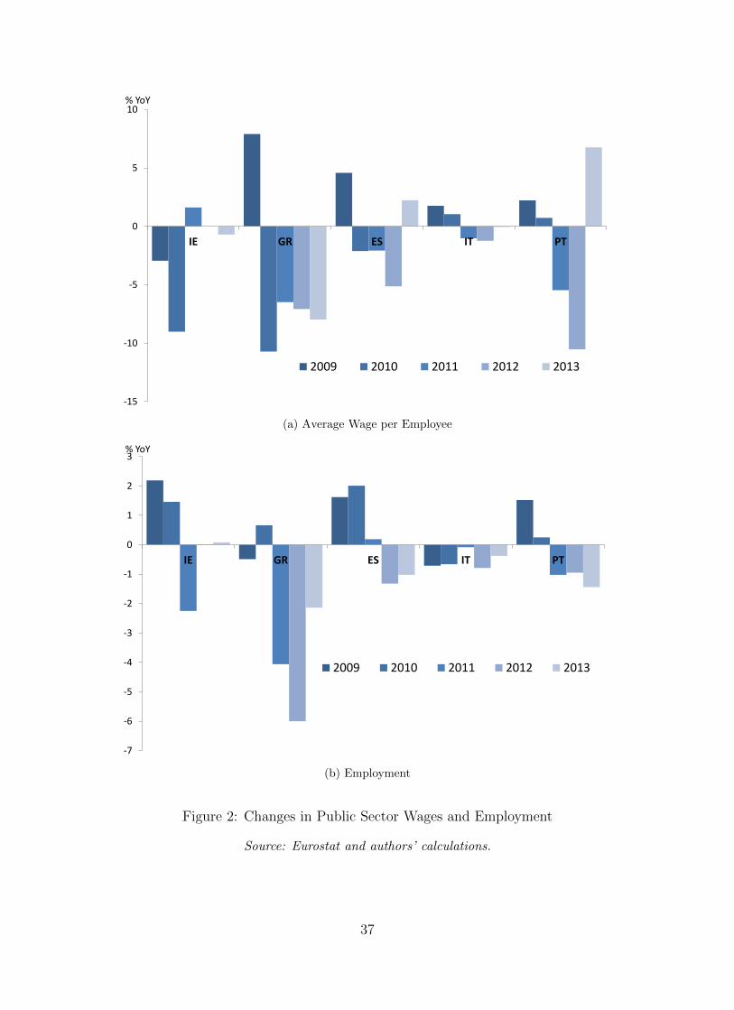
Fiscal consolidation policies implemented in the Euro area in recent years have placed special

emphasis on reducing the public wage bill, which represents a sizable component of the

government budget.1 The fall in the nominal government wage bill has been particularly

pronounced in Periphery countries of the Euro area, such as Ireland, Greece and Portugal

(see Figure 1), and has come from cuts in both wages and the number of employees in

the public sector (see Figure 2).2 At the same time, the Euro area has been experiencing

a prolonged period of inflation uncertainty: with monetary policy constrained by the zero

lower bound (ZLB henceforth), inflation has remained below the ECB’s medium run objective

for some time. This environment of low inflation has important implications for the design

and implementation of fiscal policy. This paper offers a positive analysis of the relative

effectiveness of cutting wages versus cutting hiring for reducing the public wage bill in a

monetary union when inflation is low.

Historically, periods of high inflation have been used to reduce debt-to-GDP ratios, for

example in many western countries following both the First and Second World War (Reinhart

et al. 2015). On the contrary, low inflation, all else equal, raises deficit- and debt-to-GDP

ratios by reducing the growth in nominal GDP. Debt dynamics would be left unchanged

if nominal interest rates adjust by the same magnitude as inflation, thus leaving real rates

unchanged. Instead, when nominal rates have hit the ZLB, falling inflation leads to rising

real interest rates, making it more difficult to reduce government debt-to-GDP ratios.

Recent studies, both theoretical and empirical, have looked at a less direct effect of low

inflation on fiscal policy, namely the impact of the ZLB on fiscal multipliers. Much of the

literature has found that fiscal multipliers are higher when monetary policy is constrained.3

1Before the crisis the government wage bill accounted, on average, for almost 25% of total public spendingand more than 10% of GDP, and almost 15% of the labor force in the Euro area was employed in the publicsector (see Holm-Hadulla et al. 2010).

2These policies have been implemented through reducing overtime pay, retrenching specific indemnitiesor benefits, implementing attrition rules to reduce new hiring or simply by outright lay-offs and pay cuts.In Greece, for example, a 10% cut across all public sector wages was legislated in 2010, followed by furthercuts. In Spain, the attrition rule allowed a new hire for every 10 exits.

3Eggertsson (2011), Christiano et al. (2011), Coenen et al. (2012) and De Long and Summers (2012) findthat the government spending multiplier increases significantly at the ZLB. Erceg and Linde (2013) showthat the magnitude of the output contraction induced by spending-based consolidation is roughly three timeslarger when monetary policy is constrained by the ZLB. Ilzetzki et al. (2013) report substantially highermultipliers in countries operating under fixed exchange rates, another form of constrained monetary policy.

2

Based on this principle, several papers discuss the potential role of fiscal stimulus in allevi-

ating a ZLB crisis: Correia et al. (2013) suggest a stimulus strategy based on consumption

taxation, and Rendahl (2016) focuses on how expansionary fiscal policy can best exploit the

amplification of labor market movements at the ZLB. The converse of these arguments is

that attempting to carry out fiscal consolidation in a liquidity trap can be very costly, and

even self-defeating.

Another important interaction between fiscal and monetary policy is the fact that inflation

can have a different impact, both in terms of size and timing, across different components of

public expenditure and revenue. Jalil (2012) shows that the differences between the estimated

multipliers of government spending and taxation can be explained by the differential response

of monetary policy. Erceg and Linde (2013) find that, at the ZLB, a tax-based consolidation

is less costly in the short run than a spending-based consolidation, while the opposite is

true when monetary policy is unconstrained. McManus et al. (2014) demonstrate that the

ZLB has different effects on different fiscal consolidation instruments, and should therefore

be considered when designing fiscal policy. We extend this literature by comparing the

effectiveness of two different instruments for reducing the public wage bill at the ZLB and

compare them with traditional instruments of fiscal consolidation considered in the existing

literature.

We consider a New Keynesian model of a two-block monetary union, calibrated for the

Periphery and Core of the Euro area. In order to build a complete model of the labor market,

we incorporate both search and matching frictions, leading to involuntary unemployment, and

an endogenous labor force participation decision, leading to voluntary unemployment. We

allow the government to hire public employees to produce a public good. Following Erceg

and Linde (2013) and Pappa et al. (2015), we compare a given public debt consolidation

through two alternative fiscal instruments, namely public wage cuts and public vacancy cuts,

in normal times and in a low inflation environment.4

In normal times, cuts in the public wage bill using either instrument cause a reallocation

of labor towards the private sector, facilitating hiring and leading to a fall in the private wage

4An example of fiscal consolidation through the public wage bill in normal times comes from the Germaneconomy. In 2000, spending cuts amounted in Germany to DM 30.1 billion or 0.75% of GDP, involvingmainly the public sector wage bill, social programs, and subsidies.

3

in the medium run. This induces an internal devaluation: by increasing the competitiveness

of the private sector of the Periphery, the consolidation leads to a depreciation of the real

exchange rate. Together with the positive wealth effect of the cut in government spending,

which raises private demand, this boosts private output. Both types of consolidation bring

about a fall in the unemployment rate. Public wage cuts lead to a larger fall in unemployment

as the private sector quickly absorbs the increased share of jobseekers, while public vacancy

cuts lead to a more sluggish adjustment in the labor market. Comparing with the traditional

instruments of fiscal consolidation in the existing literature, both tax hikes and spending cuts

tend to decrease private output. Tax hikes reduce labor force participation, increasing the

private wage and marginal costs for firms. Spending cuts, although they crowd-in private

consumption and investment, they induce a reduction in labor supply, which leads to a fall

in vacancies and employment in the private sector, and counterbalances the positive wealth

effect of the consolidation.

In a low inflation environment, induced by negative demand shocks and a ZLB constraint

on monetary policy, the government debt-to-GDP ratio rises, and, hence, a significantly larger

cut in the public wage bill is required. Furthermore, with the contraction in demand, the

private sector is much more limited in its ability to absorb jobseekers leaving the public sector

job search, and private employment falls during the liquidity trap. Still, the reallocation of

jobseekers after a public wage cuts quickly reverses the path of private employment by reduc-

ing labor costs, and decreases unemployment in the medium run. Public vacancy cuts do not

induce a strong reallocation of jobseekers and reduce public employment more significantly.

As a result, vacancy cuts increase unemployment in the medium run. Again, standard fiscal

instruments would deepen the recession induced by the negative demand shocks relative to

consolidation through the public wage bill.

We run a series of alternative simulations to investigate the mechanisms at play in our

model. First, we find that the ability of jobseekers to reallocate their search is of key im-

portance: rigidities in the mobility of labor between the public and private sectors mitigate

the positive effects of the fiscal consolidation on private employment after the liquidity trap,

making consolidation itself more difficult to achieve. Second, price flexibility is crucial for the

success of the fiscal consolidation at the ZLB. When the degree of price stickiness in the Pe-

4

riphery is assumed to be higher than in the Core, the internal devaluation channel is reversed,

making the consolidation harder to achieve. Third, looking at the role of the public good

in the economy, we find that consolidation in a low inflation environment is more difficult if

the public good is productive, such that the cut in public sector output has an effect on the

marginal product of private labor. Finally, concerning parameters related to the openness

of the Periphery, we show that lower elasticity of substitution between home-produced and

imported goods makes consolidation harder to achieve, whereas a bigger size of the block

implementing the consolidation implies that it becomes less costly.

Our work is related to a few recent articles. On the empirical side, our results are con-

sistent with the recent findings of Perez et al. (2016), who show that while government wage

and employment reforms have adverse short term effects, such measures can yield medium to

long term benefits due to possible competitiveness gains, through spillover effects on private

sector wages, and efficiency gains, through their impact on labor market dynamics. Another

related paper is the empirical work of Lamo et al. (2016), who find that the contractionary

effects of employment cuts appear more damaging for the Spanish economy than those of

wage cuts. Using US data, Bermperoglou et al. (2017) find that public employment shocks

are mildly expansionary at the federal level and strongly expansionary at the state and local

level by crowding in private consumption and increasing labor force participation and pri-

vate sector employment. Similarly, state and local government wage shocks lead to increases

in consumption and output, while shocks to federal government wages induce significant

contractionary effects.

On the theoretical side, the literature has also investigated the impact of shocks in the

public sector on the level and volatility of employment and wages (see e.g. Quadrini and

Trigari (2007) and Gomes (2015)). Bradley et al. (2016) estimate a structural model with a

public sector and a labor market with search and matching frictions, using UK data. The

authors run simulations of austerity measures, such as a reduction in public sector hiring, an

increase in public sector lay-offs, and progressive and proportional cuts to the distribution

of wages in the public sector, that were implemented after the 2008 recession. In line with

our results away from the ZLB, they find that all policies increase hiring and turnover in

the private sector. In an earlier contribution, Demekas and Kontolemis (2000) developed a

5

simple two-sector model of the labor market with endogenous unemployment, but without

explicit dynamics, showing that increases in government wages lead to increases in private

sector wages and higher unemployment, while increases in government employment do not

have a significant impact on unemployment. Similarly, Ardagna (2007) has shown that, in a

DSGE model with a unionized labor market, unions demand higher wages in response to a

debt-financed increase in public sector employment and wages, which leads to a fall in private

sector employment and a contraction in the economy. We extend the existing literature by

considering a DSGE model of a monetary union, and by explicitly incorporating the ZLB

and analyzing its consequences for the effects of cuts in the public wage bill.5

The remainder of the paper is organized follows. In Section 2, we provide the details of

the model. Section 3 discusses the results of the different policy experiments and Section 4

provides extensive sensitivity analysis. Section 5 concludes.

2 The Model

We consider a DSGE model of a two-block monetary union with search and matching frictions,

endogenous labor force participation, and sticky prices in the short run. The two countries,

labeled Home and Foreign, are of sizes n and 1− n, respectively. The following subsections

describe the Home economy in more detail: the structure of the Foreign economy is analogous.

All variables are in per capita terms. Where necessary, the conventional ? denotes foreign

variables or parameters, and the subscripts h and f denote goods produced in the Home and

Foreign economy and their respective prices.

There are four types of firms in each block: (i) a government-owned firm that produces

the public good, (ii) private competitive firms that use labor and effective capital to produce

a non-tradable intermediate good, (iii) monopolistic retailers that transform the intermediate

good into a tradable good, and (iv) competitive final goods producers that use domestic and

foreign produced retail goods to produce a final, non-tradable good that is used for investment

5A link can also be established with the two-country model of a currency union in Kuvshinov et al. (2016).The authors look at a deleveraging shock taking place in the Periphery and find that deleveraging generatesdeflationary spillovers which cannot be contained by monetary policy, as it becomes constrained by the zerolower bound.

6

and consumption. Price rigidities arise at the retail level, while labor market frictions occur

in the intermediate goods sector. The representative household consists of private and public

employees, unemployed, and labor force non-participants. The government collects taxes and

issues debt to finance the wages of public employees, the cost of opening new vacancies in

the public sector and the provision of unemployment benefits.

2.1 Labor markets

We consider search and matching frictions in both the private and public labor markets.

In each period, jobs in each sector, j = p, g, are destroyed at a constant fraction σj and a

measure mj of new matches are formed. The evolution of employment in each sector is thus

given by:

njt+1 = (1− σj)njt +mjt (1)

We assume that σp > σg in order to capture the fact that, in general, public employment is

more permanent than private employment.6

The new matches are given by:

mjt = µj(υjt )

µ(ujt)1−µ (2)

where υ and u are vacancies and jobseekers respectively, and the matching efficiency, µj, can

differ in the two sectors. From the matching functions specified above we can define, for each

sector j, the probability of a jobseeker being hired, ψhjt , and of a vacancy being filled, ψfjt :

ψhjt ≡mjt

ujt(3)

ψfjt ≡mjt

υjt(4)

6For example, Albrecht et al. (2015) and Gomes (2015) find empirical evidence that separation rates inthe public sector are lower than the private sector in the UK, US and Colombia, respectively.

7

2.2 Households

The representative household consists of a continuum of infinitely lived agents. The members

of the household derive utility from leisure, which corresponds to the fraction of members

that are out of the labor force, lt, and a consumption bundle, ct. The instantaneous utility

function is, thus, given by:

U(ct, lt, xt) =(ct − ζct−1)1−η

1− η+ Φ

l1−ϕt

1− ϕ(5)

where η is the inverse of the intertemporal elasticity of substitution, ζ is the parameter

determining habits in consumption, Φ > 0 is the relative preference for leisure and ϕ is the

inverse of the Frisch elasticity of labor supply.

At any point in time, a fraction npt (ngt ) of the household members are private (public)

employees. Bruckner and Pappa (2012) and Campolmi and Gnocchi (2016) have added

a labor force participation choice in New Keynesian models of equilibrium unemployment.

Following Ravn (2008), the participation choice is modeled as a trade-off between the cost

of giving up leisure and the prospect of finding a job. In particular, the household chooses

the fraction of the unemployed actively searching for a job, ut, and the fraction which are

out of the labor force and enjoying leisure, lt. Normalising the size of the household to 1, the

composition of the household is given by:

npt + ngt + ut + lt = 1 (6)

The household chooses the fraction of jobseekers searching in each sector: a share st of

jobseekers look for a job in the public sector, while the remainder, (1− st), seek employment

in the private sector. That is, ugt ≡ stut and upt ≡ (1− st)ut.

The household owns the private capital stock, which evolves according to:

kpt+1 =

[1− ω

2

(itit−1

− 1

)2]it + (1− δ(xt)) kpt (7)

where it is private investment, ω dictates the size of investment adjustment costs. Following

8

Neiss and Pappa (2005), the depreciation rate, δ(xt), will depend on the degree of capital

utilization, xt, according to:

δ(xt) = δxξt (8)

where δ and ξ are positive constants.

The budget constraint, in real terms, is given by:

(1 + τ c) ct + it + bg,t+1 + etrf,t−1bf,t ≤[rkt − τ k

(rkt − δ(xt)

)]xtk

pt + rt−1bg,t + etbf,t+1(9)

+ (1− τnt ) (wptnpt + wgtn

gt ) + but + Πp

t + Tt

where wjt , j = g, p, are the real wages in the two sectors, rkt is the real return on effective

capital, b denotes unemployment benefits, Πpt are the profits of the monopolistic retailers,

discussed below, and τ c, τ k, τnt , and Tt represent taxes on private consumption, private

capital, labor income and lump-sum transfers, respectively. Government bonds are denoted

by bg,t, and pay the real return rt−1, while bf,t denote liabilities with the Foreign country.7

Although the nominal exchange rate is fixed, the interest rate on foreign assets, rf,t, is

still affected by consumer price inflation differentials between the two countries, which are

captured by the real exchange rate, et. In fact, we can define the gross nominal interest rate

at Home, Rt, through the Fisher equation:

rt =Rt

Etπt+1

(10)

where πt is the gross consumer price inflation rate.

The problem of the household is to choose ct, ut, st, npt+1, ngt+1, it, k

pt+1, xt, bg,t+1 and

bf,t+1 to maximize lifetime utility subject to the budget constraint, (9), the law of motion of

employment in each sector, (1), taking the probability of finding a job as given, the law of

motion of capital, (7), the definition of capital depreciation, (8), and the composition of the

household, (6). The resulting first order conditions are provided in an online appendix.8

7Assuming government debt is only held by local households captures well the case of Periphery countrieslike Italy and Spain, where the largest fraction of public debt is held domestically. An interesting extensionwould be to allow for public debt to also be held externally.

8The online appendix can be found at https://me.eui.eu/evi-pappa/

9

We can derive the marginal value of an additional private sector employee as:

V Hnpt = λctw

pt (1− τnt )− Φl−ϕt + (1− σp)βEt(V

Hnpt+1) (11)

where λct is the Lagrange multiplier on the budget constraint. Using (11) together with the

equivalent expression for the value of an additional public sector employee, the definition of

hiring rates, (3), and the first order condition with respect to st, we obtain:

Et

(V Hng ,t+1

)ψhgt = Et

(V Hnp,t+1

)ψhpt (12)

This equation shows that, in equilibrium, the expected value of searching in the two sectors is

equalized. This expected value will depend not only on the probability of finding a job in each

sector, ψhjt , but also on the expected utility from having an additional worker in each sector,

which, in turn, will depend on the respective wage in each sector and the separation rate, σj.

This means that a wage differential can arise between the two sectors in a non-degenerate

equilibrium if there are differences in the number of vacancies, the matching efficiency, or the

separation rate.

2.3 Production

2.3.1 Intermediate goods firms

Intermediate goods are produced with a Cobb-Douglas technology:

ypt = (npt )1−φ(xtk

pt )φ (13)

where kpt and npt are private capital and labor inputs, and xt is the degree of capital utiliza-

tion.9

9The assumption of variable capital utilization here is important: note that, without it, all factors ofproduction would be predetermined, meaning that output cannot adjust on impact in response to shocks. Inthis case, the nominal interest rate needs to adjust sharply to bring the economy to equilibrium. To illustratethis, we present, in the appendix, the results of our model without variable capital utilization away from theZLB.

10

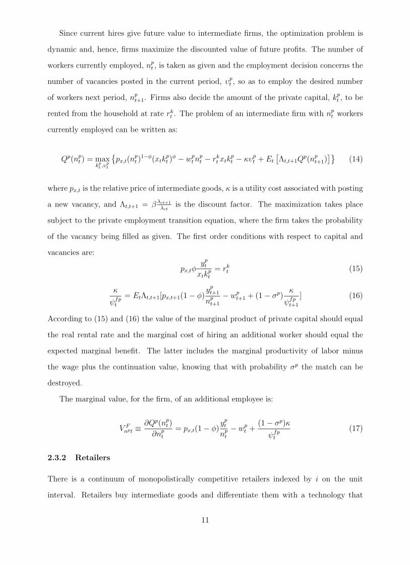
Since current hires give future value to intermediate firms, the optimization problem is

dynamic and, hence, firms maximize the discounted value of future profits. The number of

workers currently employed, npt , is taken as given and the employment decision concerns the

number of vacancies posted in the current period, υpt , so as to employ the desired number

of workers next period, npt+1. Firms also decide the amount of the private capital, kpt , to be

rented from the household at rate rkt . The problem of an intermediate firm with npt workers

currently employed can be written as:

Qp(npt ) = maxkpt ,υ

pt

{px,t(n

pt )

1−φ(xtkpt )φ − wptn

pt − rkt xtk

pt − κυ

pt + Et

[Λt,t+1Q

p(npt+1)]}

(14)

where px,t is the relative price of intermediate goods, κ is a utility cost associated with posting

a new vacancy, and Λt,t+1 = β λct+1

λctis the discount factor. The maximization takes place

subject to the private employment transition equation, where the firm takes the probability

of the vacancy being filled as given. The first order conditions with respect to capital and

vacancies are:

px,tφyptxtk

pt

= rkt (15)

κ

ψfpt= EtΛt,t+1[px,t+1(1− φ)

ypt+1

npt+1

− wpt+1 + (1− σp) κ

ψfpt+1

] (16)

According to (15) and (16) the value of the marginal product of private capital should equal

the real rental rate and the marginal cost of hiring an additional worker should equal the

expected marginal benefit. The latter includes the marginal productivity of labor minus

the wage plus the continuation value, knowing that with probability σp the match can be

destroyed.

The marginal value, for the firm, of an additional employee is:

V Fnpt ≡

∂Qp(npt )

∂npt= px,t(1− φ)

yptnpt− wpt +

(1− σp)κψfpt

(17)

2.3.2 Retailers

There is a continuum of monopolistically competitive retailers indexed by i on the unit

interval. Retailers buy intermediate goods and differentiate them with a technology that

11

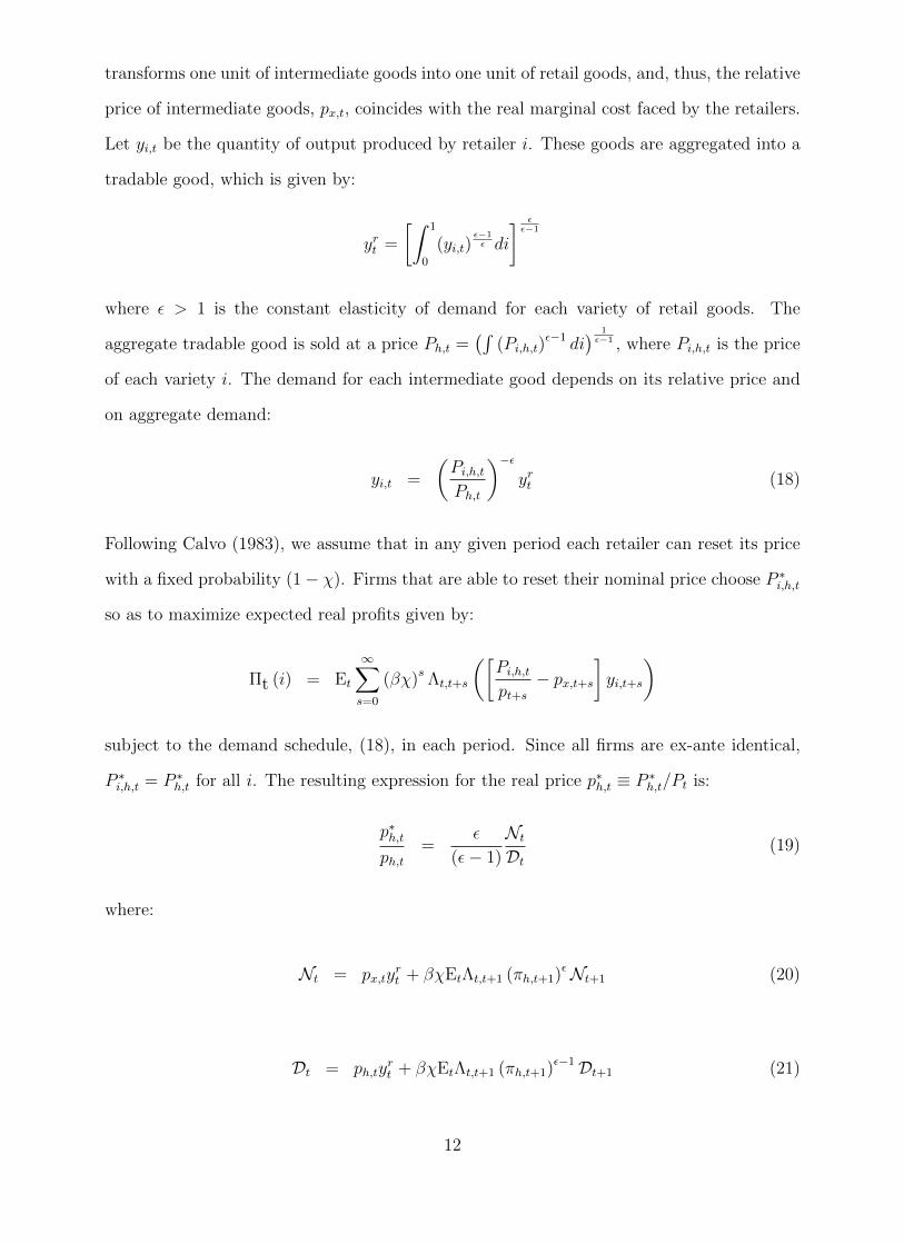
transforms one unit of intermediate goods into one unit of retail goods, and, thus, the relative

price of intermediate goods, px,t, coincides with the real marginal cost faced by the retailers.

Let yi,t be the quantity of output produced by retailer i. These goods are aggregated into a

tradable good, which is given by:

yrt =

[∫ 1

0

(yi,t)ε−1ε di

] εε−1

where ε > 1 is the constant elasticity of demand for each variety of retail goods. The

aggregate tradable good is sold at a price Ph,t =(∫

(Pi,h,t)ε−1 di

) 1ε−1 , where Pi,h,t is the price

of each variety i. The demand for each intermediate good depends on its relative price and

on aggregate demand:

yi,t =

(Pi,h,tPh,t

)−εyrt (18)

Following Calvo (1983), we assume that in any given period each retailer can reset its price

with a fixed probability (1− χ). Firms that are able to reset their nominal price choose P ∗i,h,t

so as to maximize expected real profits given by:

Πt (i) = Et

∞∑s=0

(βχ)s Λt,t+s

([Pi,h,tpt+s

− px,t+s]yi,t+s

)

subject to the demand schedule, (18), in each period. Since all firms are ex-ante identical,

P ∗i,h,t = P ∗h,t for all i. The resulting expression for the real price p∗h,t ≡ P ∗h,t/Pt is:

p∗h,tph,t

=ε

(ε− 1)

NtDt

(19)

where:

Nt = px,tyrt + βχEtΛt,t+1 (πh,t+1)εNt+1 (20)

Dt = ph,tyrt + βχEtΛt,t+1 (πh,t+1)ε−1Dt+1 (21)

12

ph,t ≡ Ph,t/Pt and πh,t denotes producer price inflation. Under the assumption of Calvo

pricing, the price index, in nominal terms, is given by:

(Ph,t)1−ε = χ (Ph,t−1)1−ε + (1− χ)

(P ∗h,t)1−ε

(22)

The aggregate tradable good is sold domestically and abroad:

yrt = yh,t + y?h,t (23)

where yh,t is the quantity of tradable goods sold domestically and y?h,t the quantity sold

abroad, and we have assumed the law of one price holds:

ph,t = etp?h,t (24)

2.3.3 Final Goods Producer

Finally, in each block, perfectly competitive firms produce a non-tradable final good by

aggregating domestic and foreign aggregate retail goods using CES technology:

yt =[($)

1γ (yh,t)

γ−1γ + (1−$)

1γ (τyf,t)

γ−1γ

] γγ−1

where τ ≡ (1− n) /n normalizes the amount of imported goods at Home to per capita terms.

The home bias parameter, $, denotes the fraction of the final good that is produced at

home. The elasticity of substitution between home-produced and imported goods is given

by γ. Final good producers maximize profits yt − ph,tyh,t − pf,tτyf,t each period. Solving for

the optimal demand functions gives:

yh,t = $ (ph,t)−γ yt (25)

yf,t = (1−$) (pf,t)−γ 1

τyt (26)

13

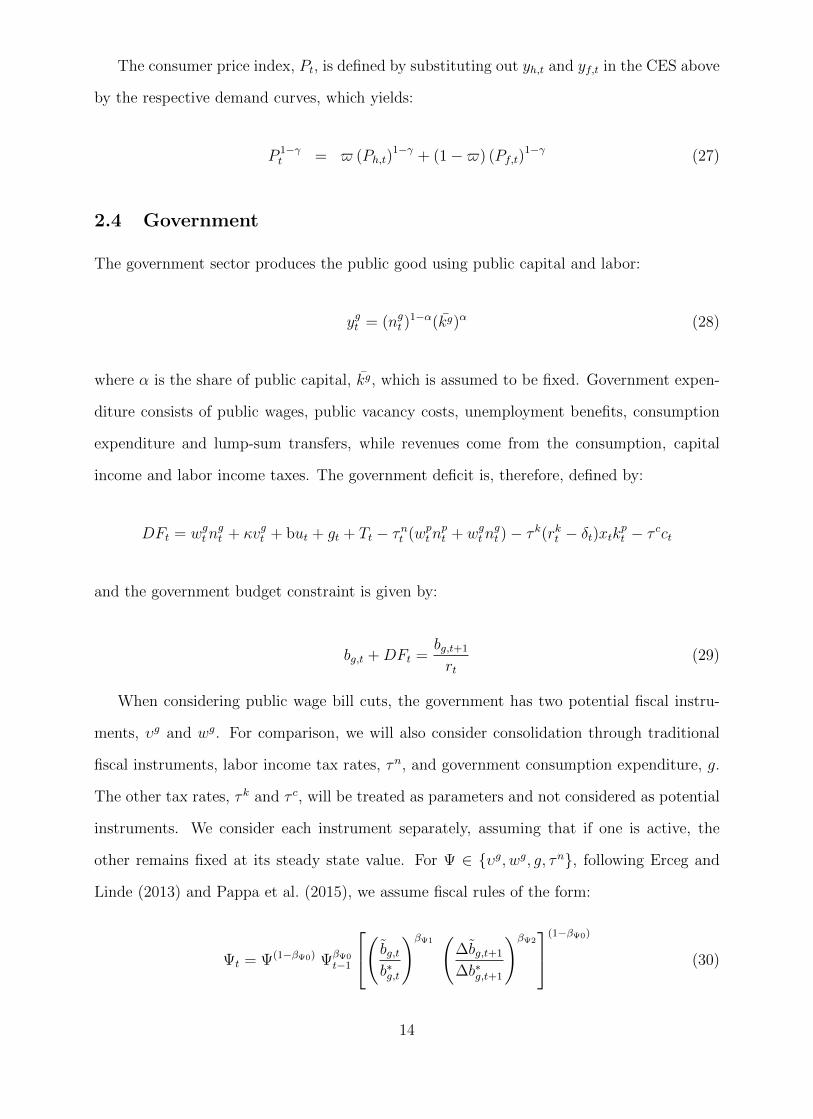
The consumer price index, Pt, is defined by substituting out yh,t and yf,t in the CES above

by the respective demand curves, which yields:

P 1−γt = $ (Ph,t)

1−γ + (1−$) (Pf,t)1−γ (27)

2.4 Government

The government sector produces the public good using public capital and labor:

ygt = (ngt )1−α(kg)α (28)

where α is the share of public capital, kg, which is assumed to be fixed. Government expen-

diture consists of public wages, public vacancy costs, unemployment benefits, consumption

expenditure and lump-sum transfers, while revenues come from the consumption, capital

income and labor income taxes. The government deficit is, therefore, defined by:

DFt = wgtngt + κvgt + but + gt + Tt − τnt (wptn

pt + wgtn

gt )− τ k(rkt − δt)xtk

pt − τ cct

and the government budget constraint is given by:

bg,t +DFt =bg,t+1

rt(29)

When considering public wage bill cuts, the government has two potential fiscal instru-

ments, υg and wg. For comparison, we will also consider consolidation through traditional

fiscal instruments, labor income tax rates, τn, and government consumption expenditure, g.

The other tax rates, τ k and τ c, will be treated as parameters and not considered as potential

instruments. We consider each instrument separately, assuming that if one is active, the

other remains fixed at its steady state value. For Ψ ∈ {υg, wg, g, τn}, following Erceg and

Linde (2013) and Pappa et al. (2015), we assume fiscal rules of the form:

Ψt = Ψ(1−βΨ0) ΨβΨ0t−1

( bg,tb∗g,t

)βΨ1(

∆bg,t+1

∆b∗g,t+1

)βΨ2

(1−βΨ0)

(30)

14

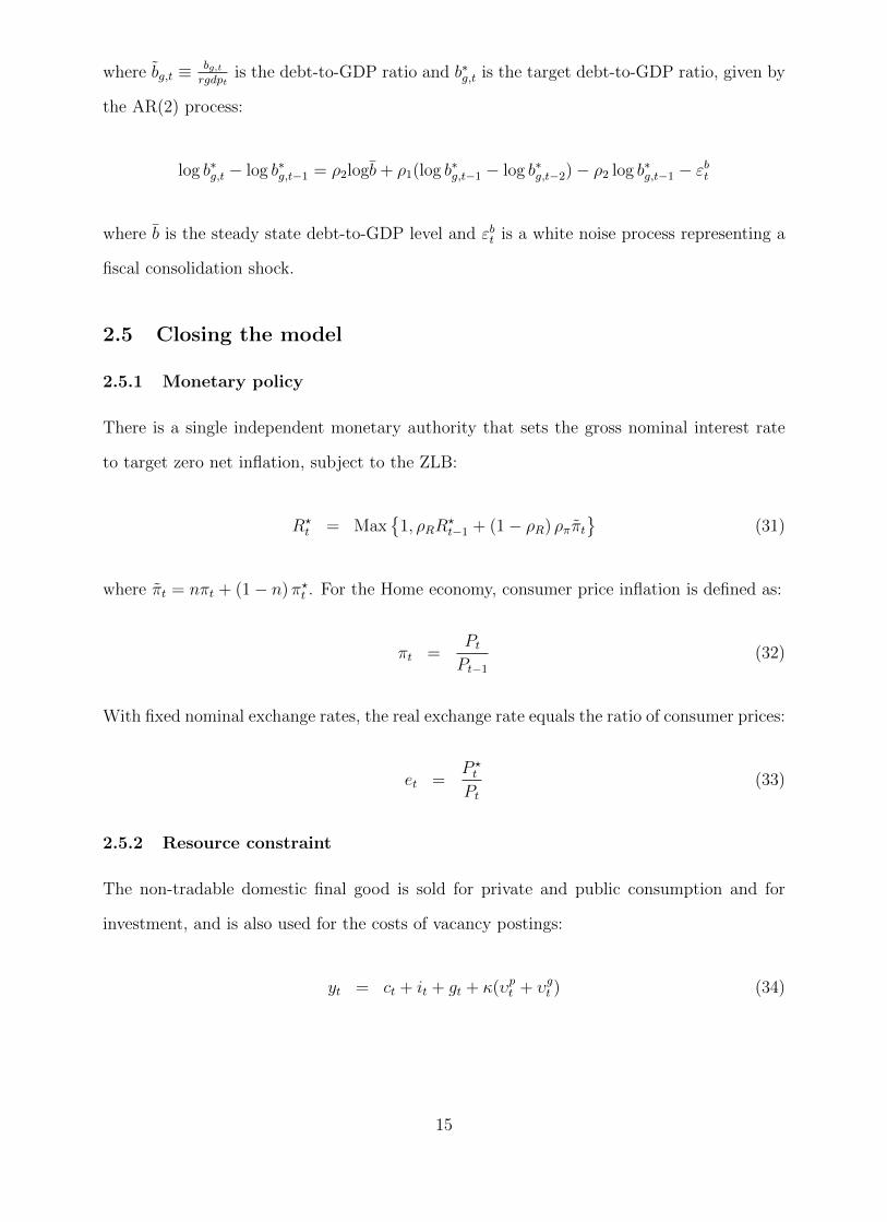
where bg,t ≡ bg,trgdpt

is the debt-to-GDP ratio and b∗g,t is the target debt-to-GDP ratio, given by

the AR(2) process:

log b∗g,t − log b∗g,t−1 = ρ2logb+ ρ1(log b∗g,t−1 − log b∗g,t−2)− ρ2 log b∗g,t−1 − εbt

where b is the steady state debt-to-GDP level and εbt is a white noise process representing a

fiscal consolidation shock.

2.5 Closing the model

2.5.1 Monetary policy

There is a single independent monetary authority that sets the gross nominal interest rate

to target zero net inflation, subject to the ZLB:

R?t = Max

{1, ρRR

?t−1 + (1− ρR) ρππt

}(31)

where πt = nπt + (1− n) π?t . For the Home economy, consumer price inflation is defined as:

πt =PtPt−1

(32)

With fixed nominal exchange rates, the real exchange rate equals the ratio of consumer prices:

et =P ?t

Pt(33)

2.5.2 Resource constraint

The non-tradable domestic final good is sold for private and public consumption and for

investment, and is also used for the costs of vacancy postings:

yt = ct + it + gt + κ(υpt + υgt ) (34)

15

In turn, following the national accounting identity, total output is defined as tradable output

plus the government wage bill:

rgdpt = ph,tyrt + wgtn

gt (35)

Aggregating the budget constraint of households using the market clearing conditions,

the budget constraint of the government, and aggregate profits, we obtain the law of motion

for net foreign assets, which is given by:

et (rf,t−1bf,t − bf,t+1) = nxt (36)

and where nxt are net exports defined as:

nxt = ph,ty?h,t − pf,tτyf,t (37)

Finally, we introduce a risk premium charged to Home households depending on the

relative size of net foreign liabilities to real GDP:

rf,t = r?t exp

{Γet

bf,t+1

rgdpt

}(38)

where Γ is the elasticity of the risk premium with respect to the liabilities.

2.5.3 Wage bargaining

Private sector wages are determined by ex post (after matching) Nash bargaining. Workers

and firms split rents and the part of the surplus they receive depends on their bargaining

power. Denoting by ϑ ∈ (0, 1) the firms’ bargaining power, the Nash bargaining problem is

to maximize the weighted sum of log surpluses:

maxwpt

{(1− ϑ) lnV H

npt + ϑ lnV Fnpt

}

16

where V Hnpt and V F

npt are given by (11) and (17), respectively. The optimization problem leads

to the following solution for wpt :

wpt = (1− ϑ)px,t(1− φ)yptnpt

+ϑ

(1− τnt )λc,tΦl−ϕt (39)

Hence, the equilibrium wage is a weighted average of the marginal product of employment

and the disutility from labor, with the weights given by the firm and household’s bargaining

power, respectively.

2.6 Model Solution and Calibration

We solve the model by linearizing the equilibrium conditions around a non-stochastic steady

state in which all prices are flexible, the price of the private good is normalized to unity,

and inflation is zero. To account for the ZLB, which is a non-linear constraint, we use the

Occbin toolkit provided by Guerrieri and Iacoviello (2015). Following the literature, the

low inflation environment is induced by assuming a shock to the household’s discount rate,

%βt , in both countries. This shock contracts demand and causes inflation to fall across the

monetary union, driving the common nominal interest rate to its lower bound. By raising the

household’s propensity to save, the discount factor shock by itself induces a rise in investment.

To avoid this counterfactual behavior for investment, we also introduce a shock to the price

of investment, %it, that leads to a fall in investment.10

The stochastic processes for these fluctuations are as follows:

%βt = (1− ρβ)%β + ρβ%βt−1 + εβt

%it = (1− ρi)%i + ρi%it−1 + εit

where we set ρβ = 0.6 and ρi = 0.85.

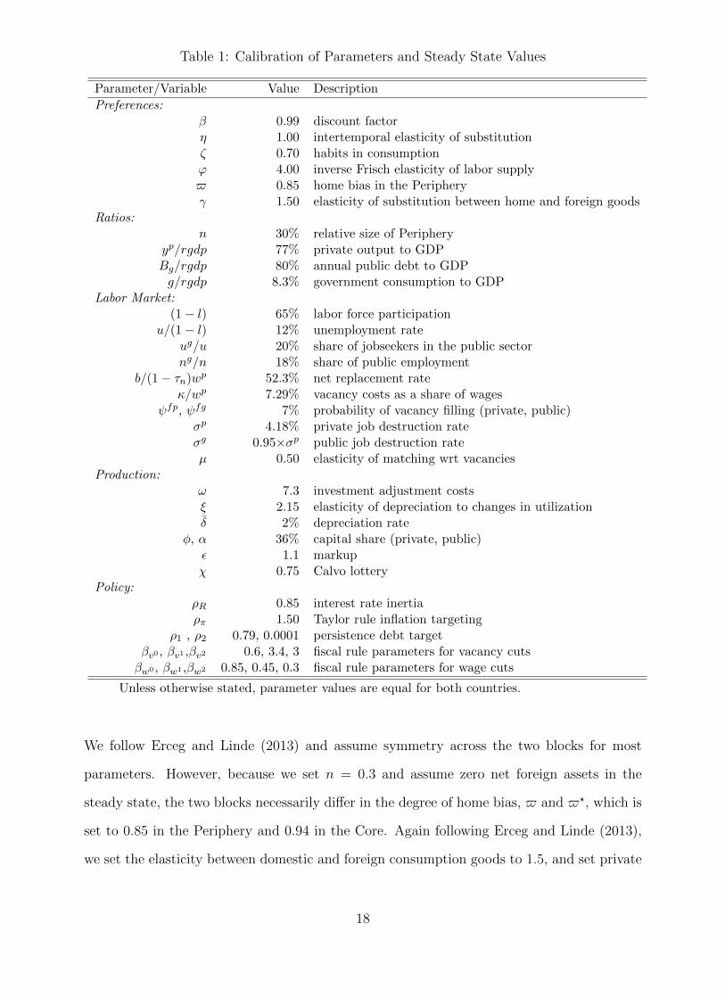
Table 1 shows the key parameters and steady state values targeted in our calibration. We

calibrate the model at a quarterly frequency and consider the Home economy to represent

the Periphery of the Euro area, consisting of Greece, Ireland, Italy, Portugal and Spain.

10Responses for the low inflation environment without the investment shock are shown in the online ap-pendix. The responses of variables other than investment are not qualitatively affected by this shock.

17

Table 1: Calibration of Parameters and Steady State Values

Parameter/Variable Value Description

Preferences:β 0.99 discount factorη 1.00 intertemporal elasticity of substitutionζ 0.70 habits in consumptionϕ 4.00 inverse Frisch elasticity of labor supply$ 0.85 home bias in the Peripheryγ 1.50 elasticity of substitution between home and foreign goods

Ratios:n 30% relative size of Periphery

yp/rgdp 77% private output to GDPBg/rgdp 80% annual public debt to GDPg/rgdp 8.3% government consumption to GDP

Labor Market:(1− l) 65% labor force participation

u/(1− l) 12% unemployment rateug/u 20% share of jobseekers in the public sectorng/n 18% share of public employment

b/(1− τn)wp 52.3% net replacement rateκ/wp 7.29% vacancy costs as a share of wages

ψfp, ψfg 7% probability of vacancy filling (private, public)σp 4.18% private job destruction rateσg 0.95×σp public job destruction rateµ 0.50 elasticity of matching wrt vacancies

Production:ω 7.3 investment adjustment costsξ 2.15 elasticity of depreciation to changes in utilizationδ 2% depreciation rate

φ, α 36% capital share (private, public)ε 1.1 markupχ 0.75 Calvo lottery

Policy:ρR 0.85 interest rate inertiaρπ 1.50 Taylor rule inflation targeting

ρ1 , ρ2 0.79, 0.0001 persistence debt targetβv0 , βv1 ,βv2 0.6, 3.4, 3 fiscal rule parameters for vacancy cutsβw0 , βw1 ,βw2 0.85, 0.45, 0.3 fiscal rule parameters for wage cuts

Unless otherwise stated, parameter values are equal for both countries.

We follow Erceg and Linde (2013) and assume symmetry across the two blocks for most

parameters. However, because we set n = 0.3 and assume zero net foreign assets in the

steady state, the two blocks necessarily differ in the degree of home bias, $ and $?, which is

set to 0.85 in the Periphery and 0.94 in the Core. Again following Erceg and Linde (2013),

we set the elasticity between domestic and foreign consumption goods to 1.5, and set private

18

output, yp, to represent 77% of GDP.

We choose an annual government debt-to-GDP ratio of 80%, significantly above the Maas-

tricht limit and, therefore, consistent with an environment in which fiscal consolidation is

deemed necessary. We set the share of government consumption to GDP equal to the average

share of government intermediate consumption to GDP in the European Periphery. We set

the steady state labor income tax rate at 30%, and set government consumption expenditure

at 80% of the public wage bill, in line with the euro area average.

The rest of the utility function parameters are standard. The intertemporal elasticity

of substitution is set to 1 and the habit parameter is set equal to 0.6 in order to increase

persistence and the duration of the lower bound. We assume a Frisch elasticity of labor

supply equal to 0.25.

We set the labor force participation rate to 65%, assume that 20% of jobseekers are search-

ing in the public sector, and that 18% of employed workers are working for the government.

For the remaining labor market parameters, we follow Moyen et al. (2016), who calibrate a

model for the Euro area with one block matching the Periphery. As such, the unemployment

rate is set to 12%, the net replacement rate to equal 52.3% and vacancy posting costs to

represent 7.29% of private wages. We assume equal probabilities of a vacancy to be filled in

both sectors, ψfp = ψfg = 7%. As discussed above, we assume that the average duration

of employment is shorter in the private sector, and therefore set the separation rate in the

public sector 5% lower than in the private sector.

The parameters in the production function are standard: the capital share is set to 0.36 in

both sectors. The depreciation rate implies an annual depreciation of 10% and the investment

adjustment costs are set equal to 7.3.11 We set the elasticity of capital depreciation to capital

utilization, ξ, such that capital utilization is 1 at steady state. Finally, we assume prices are

sticky for four quarters and that the central bank reacts only to deviations of inflation.

For the parameters governing fiscal policy, we set ρ1 and ρ2, which govern the path of the

debt-to-GDP target, such that any change in the target is observed fully after 30 quarters

and lasts for an arbitrarily long period of time, beyond the relevant policy horizon. Finally,

11We have investigated the sensitivity of our results to changes in this parameter. Lower values of ω implya higher initial drop in investment after the shock to its price and makes consolidation tougher for bothinstruments.

19

we set the parameters governing the fiscal instruments in equation (30) such that, in normal

times, the actual debt-to-GDP ratio meets the target after 30 quarters for both instruments.

3 Fiscal Consolidation through the Wage Bill

We consider a shock that drives the debt-to-GDP target 10% below its steady state. We

simulate the responses to this shock with either public vacancies, υg, or public wages, wg,

adjusting to achieve fiscal consolidation, and compare the effects of the consolidation under

these two instruments and under two alternative instruments, namely public consumption

spending, gt, and the labor income tax rate, τnt , for the sake of comparison with the existing

literature. We first look at the effects of this shock in normal times, and then compare these

results to when the consolidation is implemented in a low inflation environment.

3.1 Consolidation in Normal Times

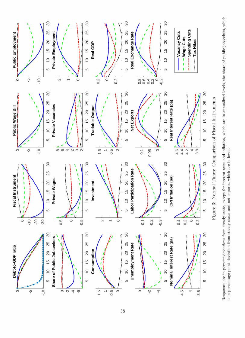
Figure 3 presents the comparison between cutting public vacancies and cutting public wages

to meet the new debt-to-GDP target, when the economy is not subject to the demand

shocks.12 For both instruments, the consolidation induces a gradual fall in the public wage

bill, and a contraction in public employment and, hence, public output. In the case of public

vacancies, the reduction in the public wage bill has a slight lag relative to the wage cuts,

due to the lag in the adjustment of public employment. Crucially, for both instruments,

the share of public sector jobseekers in total jobseekers falls. In the case of public vacancy

cuts, there is a fall in the number of matches, and hence the probability of finding a job

in the public sector. The public wage cuts cause the value of the public sector job, in the

case of a match, to fall. As a result, in both cases, the expected value of searching for a job

in the public sector is reduced. Since agents redirect their search until the expected value

of searching in each sector is equalized, this leads to a reallocation of jobseekers towards

the private sector.13 With public wages as the active instrument, this mechanism induces

12All responses are in percent deviations from steady state, except for interest rates and inflation, whichare in annualized levels, the share of public jobseekers, which is in percentage point deviation from steadystate, and net exports, which are in levels.

13Note that, in equilibrium, the expected value of searching for a job will be lower in both sectors.

20

an endogenous reduction in public employment, which further aids the consolidation. In

contrast, public vacancies need to adjust a lot more to achieve a similar fall in the public

wage bill, since in this case public wages are assumed to be fixed.

The reduction in expenditure on the public wage bill creates a positive wealth effect

for the household, which leads to falling labor force participation and hence lower labor

supply. In the short run, this raises private wages. Nonetheless, the increase in the supply

of labor in the private sector, due to the reallocation of jobseekers, eventually pushes down

on private wages. Hence, by increasing the competitiveness of the Periphery within the

monetary union, consolidation induces an internal devaluation, and so implies a depreciation

of the real exchange rate and eventually a rise in net exports.

The rise in demand for the private good, and the fall in private wages, also imply a rise

in private vacancies. The expansion of both the demand and supply of private labor raises

private employment. As the labor markets adjust, the faster response of private employment

in the case of public wage cuts means that remaining jobseekers are absorbed into private

employees, and unemployment continues to fall. On the other hand, in the case of vacancy

cuts, the sluggish response of the private sector labor market means that fewer jobseekers

are hired. Along with the fact that public employment falls by much more in the medium

to long run, this implies that the unemployment rate falls less noticeably when vacancy cuts

are the active instrument.

Recalling the definition of GDP as the sum of private and public output, with the latter

measured by the public wage bill, we can see that the consolidation process initially boosts

GDP following the increase in private sector output, but then depresses GDP for many

periods, given the fall in the public wage bill. In the short to medium run, this effect is

somewhat bigger for wage cuts, given the larger increase in tradable output. The long run

effect on tradable output is higher for vacancy cuts, which mitigates the fall in real GDP

relative to public wage cuts.

Although our model differs substantially from Bradley et al. (2016), we also find that in

normal times cuts in the public wage bill expand the private sector, both by raising demand

and causing a reallocation of jobseekers to the private sector. We have also underlined

an additional mechanism not considered in Bradley et al. (2016), namely that for both

21

instruments the public wage bill cut in a monetary union induces an internal devaluation,

therefore aiding the recovery by raising external demand. Comparing the two instruments,

cutting public wages implies a faster expansion in the private sector, and hence a larger fall in

unemployment. Public vacancy cuts, on the other hand, imply an overall larger cut in public

employment and a significantly more sluggish response of workers, such that the positive

effects in the private sector take longer to materialize.

To gain some more insight about the nature of the consolidation we consider relative to

the existing literature, we also plot in Figure 3 the responses of the economy when debt con-

solidation is achieved through the traditional fiscal instruments, namely public consumption

spending and labor income taxes. With both wages and vacancies in the public sector kept

fixed, these alternative instruments do not affect public employment or the allocation of job-

seekers in the two sectors. In the case of government spending cuts, there is a positive wealth

effect that leads to an increase in private consumption and a fall in labor force participation,

as in the case of public wage bill cuts. The exit of jobseekers from the labor force also lowers

the unemployment rate. This inward shift in labor supply induces an increase in real wages

and firms’ marginal costs which, together with the fall in spending, induces labor demand,

and therefore private vacancies, to fall. Coupled with the fact that unemployed jobseekers

do not switch sector, this induces a fall in private employment, and hence in tradable output

and real GDP. As standard in the existing literature, and in contrast to cuts to the public

wage bill, government spending multipliers are found to be positive.

The rise in the labor tax rate also lowers labor force participation substantially, by directly

reducing the incentives to work. Since consumption also falls in this case, given the drop in

after-tax income, this leads to a bigger drop in private vacancies, and hence larger negative

effects on private employment and tradable output. Responses are significantly larger and

more persistent than in the case of consumption spending cuts, due to a fall in investment.

Furthermore, the rise in labor taxes increases unemployment after the short run and reduces

the competitiveness of the Periphery leading to a real exchange rate appreciation, unlike all

of the spending based consolidations.

22

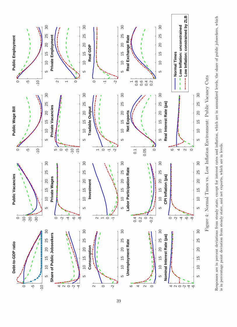
3.2 Consolidation in a Low Inflation Environment

We now turn to the case where the consolidation occurs while monetary policy is constrained

at the ZLB and inflation is stuck below steady state. Figures 4 and 5 plot the IRFs for

vacancy cuts and wage cuts, respectively. In each figure, to aid comparison, we again plot

the baseline consolidation in normal times in the blue solid lines, as in Figure 3.

For completeness, we also plot the case where the economy is hit by the negative demand

shocks but the ZLB constraint is not imposed: these are the green dashed lines. In both

Figures, in this unconstrained case the net nominal interest rate becomes negative for around

five quarters. This depresses the real interest rate, offsetting the effects of the negative

demand shocks through a smaller fall in private consumption and investment. It is interesting

to note that the fall in the real interest rate is actually a boost to public finances, and

the government’s debt-to-GDP ratio quickly falls close to the target with only a smaller

adjustment in the fiscal instruments needed.

Conversely, when the ZLB is imposed, shown by the red dash-dotted lines, the nominal

rate remains at its lower bound for around five quarters: the real interest rate is higher

than the unconstrained case and inflation falls by more. The contraction of tradable output,

coupled with the fall in inflation, push the government’s debt-to-GDP ratio in an upward

trajectory, in spite of the consolidation. Hence, a much larger adjustment of the fiscal in-

strument is needed in this environment, and in fact the target is not fully reached after 30

quarters.

At the ZLB, with both consumption and investment contracting, private vacancies fall

sharply and the private sector is no longer able to absorb the increasing number of private

jobseekers. In fact, the share of jobseekers in the public sector rises on impact in the case

of cuts in public vacancies. As a result, in the short run, private employment falls and the

unemployment rate rises, in line with the recent experience of countries in the Periphery of

the Euro area. As the consolidation in the public sector deepens, in the medium to long

run, we again see a shift of jobseekers to the private sector, a rise in private vacancies, and a

rise in private employment. Tradable output follows a similar path, contracting in the short

to medium run, but rising above steady state in the long run. Real GDP also falls sharply

23

during the liquidity trap, and remains persistently below steady state due to the larger fall

in the public wage bill.

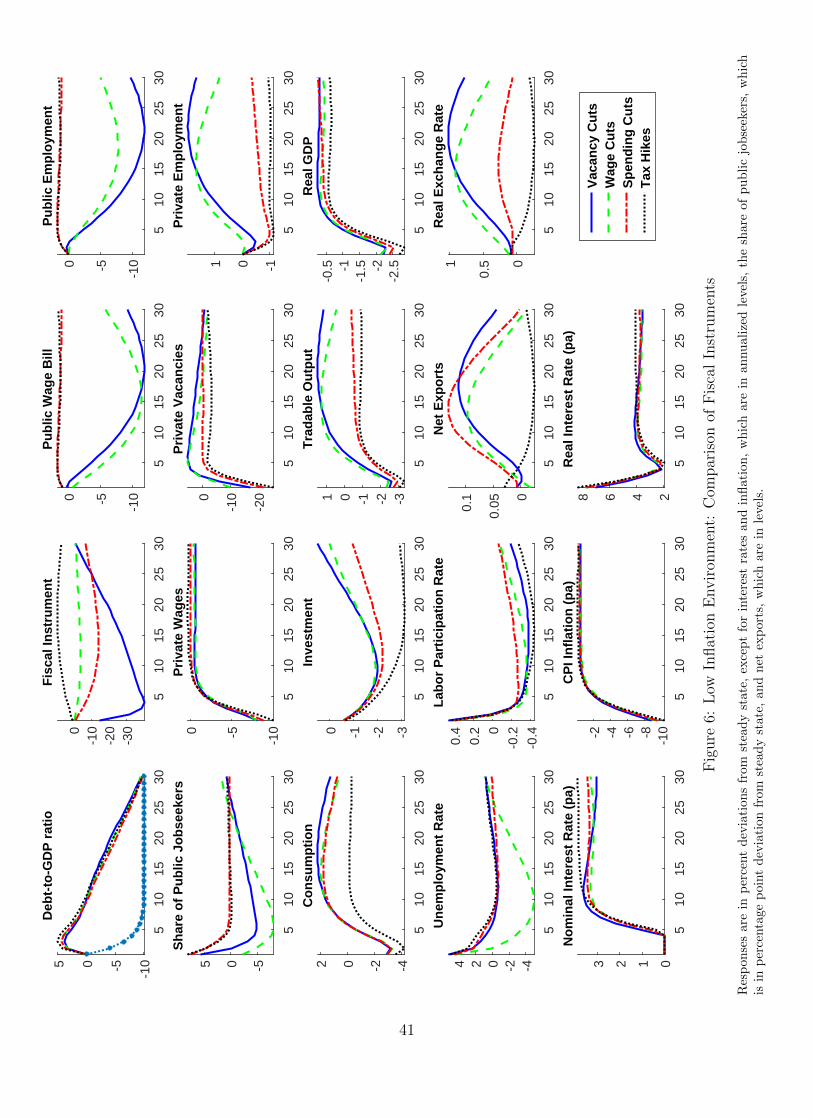
What does the low inflation environment imply about the comparison of fiscal instru-

ments? In Figure 6 we plot together the responses for the diferent instruments when the

ZLB constraint is binding. Compared to Figure 3, we see that the responses for cuts in

public vacancies and cuts in public wages are now relatively closer in general, and, particu-

larly, for tradable output and real GDP. This comes about because the relatively larger size

of the demand shocks dominates the shape of most responses. The most striking difference

is in unemployment: after the impact period, the unemployment rate falls substantially in

the case of wage cuts, while it remains elevated in the case of vacancy cuts. This difference

stems mainly from the weaker performance of private employment, and the larger fall in

public employment. Hence, in terms of the response of unemployment and the private sector

employment, the effects of public wage cuts are less adverse than those of vacancy cuts in a

low inflation environment.14

Again, in Figure 6 we compare consolidation in the public wage bill with consolidations

through standard cuts in government consumption or tax hikes. As we have seen above,

when the consolidation is implemented at the ZLB, the fall in demand causes a contraction

in the private sector, pushing down on both private sector wages and vacancies. When wages

and vacancies in the public sector do not adjust, this increases the incentives of jobseekers to

search in the public sector, and we see a sizable reallocation of labor towards the public sector.

This leads to large and persistent fall in both private employment and tradable output with

the traditional fiscal instruments. Hence, in a low inflation environment, the contraction in

the public sector through cuts in public vacancies or public wages helps the economy recover

in the medium run, while traditional consolidation instruments do not.

14In exercises we do not show here for economy of space, we find that the increase in unemploymentfollowing vacancy cuts can be mitigated by assuming a lower Frisch elasticity. Nonetheless, these results arerobust for reasonable values, 0.1 ≤ 1

ϕ ≤ 1, and do not affect our conclusions regarding the effects of wagecuts versus vacancy cuts for reducing the unemployment rate.

24

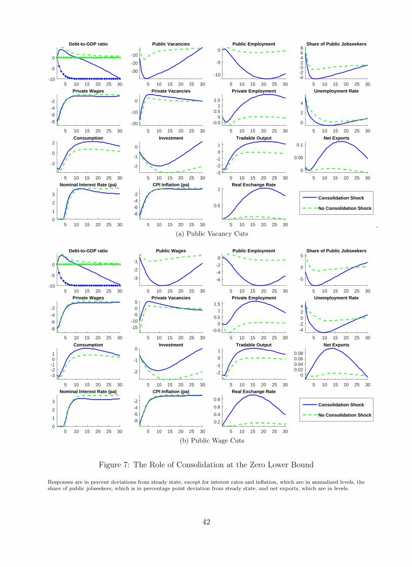
3.3 The Role of the Consolidation Shock

Since we are considering simultaneous shocks, it is useful to separate their effects. To this

end, we now compare the responses of the economy at the ZLB, as discussed above, to a case

where the economy hits the ZLB but the public debt target is held constant. The comparison

is shown in Figures 7a and 7b for vacancy cuts and wage cuts, respectively, with the blue

solid lines reporting the scenario with the consolidation shock and the green dashed lines the

one without.

For both policy instruments, consolidation is, in fact, induced by the negative demand

shocks alone. As discussed above, by inducing a fall in inflation and a contraction in the

private sector, the demand shocks increase the debt-to-GDP ratio above the target. As a

result, and according to the fiscal rule specified in equation (30), public vacancies or wages

are automatically cut, even without the fall in the debt-to-GDP target. Nonetheless, these

cuts are smaller compared to the scenario with the consolidation shock. Importantly, this

means that there is a smaller reallocation of jobseekers to the private sector after the initial

impact of the negative demand shocks. Due to the drop in private demand, now households

initially reallocate jobseekers towards the public sector for both instruments. This leads to a

smaller depreciation of the real exchange rate, and a bigger fall in private consumption. The

fall in investment is also noticeably larger. The response of private employment now becomes

persistently negative. Along with the implied smaller drop in labor force participation, this

means that, for both instruments, the unemployment rate is higher without the consolidation

shock, too. Hence, we conclude that at the ZLB the consolidation shock aids the recovery of

the economy.

4 Sensitivity Analysis

We now perform different exercises to investigate how the mechanisms of the model affect

our results at the ZLB. First, we explore the role of labor market rigidities, by assuming that

the household cannot reallocate jobseekers between the two sectors.15 Second, we investigate

15We have also investigated the effects of wage rigidity in the private sector, assuming that private realwages evolve as in Monacelli et al. (2010). These results are available in the online appendix. In line withKrause and Lubik (2007), sticky wages do not seem to substantially affect any of our previous conclusions.

25

the importance of price rigidities for the effects of fiscal consolidation. Third, we consider

the alternative scenario in which the public good is used in private production. Finally, we

test the sensitivity of our results with regards to the parameters that determine the openness

of the economy.

4.1 Fixed Allocation of Jobseekers

Our analysis has highlighted the role of the labor market channels in driving the effects of

fiscal consolidation through public wage bill cuts. We now explore the extent to which mut-

ing the reallocation of unemployed jobseekers between the two sectors, affects our findings.

Letting households choose the fraction of unemployed workers that look for a job in each of

the two sectors is important for the dynamics of our model. This assumption implies that

jobseekers can costlessly optimize their search between sectors in each period. However, in

reality, human capital derived from learned skills, past experience and in-job networking in-

troduce an asymmetry to the mobility of workers. Hence jobseekers with previous experience

in one sector would find it more difficult to be hired in the other. To explore the conse-

quences of imperfect mobility, we impose that the fraction of jobseekers in the public sector,

st, is held fixed at steady state. Hence, although the number of workers employed in each

sector can evolve separately through the dynamics of vacancy postings, matches, and labor

force participation, households cannot freely decide to reallocate jobseekers to one particular

sector.

The green dashed lines in Figures 8a and 8b depict the responses under this scenario.

With no reallocation of jobseekers to the private sector, the recovery is now much slower.

Firstly, as debt-to-GDP falls more slowly after the liquidity trap, larger and more persistent

cuts in public vacancies and wages are needed for consolidation. In fact, the target now takes

significantly longer to be met. Output and unemployment effects become more adverse. This

mechanism is particularly important for wage cuts, where, without the rise of jobseekers in the

private sector, private employment now does not increase. Nonetheless, the unemployment

rate continues to fall, since public employment does not fall, and labor force participation

falls persistently, as lower wages mean that household members find it optimal to stay at

26

home and enjoy leisure.

Overall, rigidities in the reallocation of jobseekers from the public to the private sector

imply that fiscal consolidation through cuts in the public wage bill is more difficult to imple-

ment, and comes at the cost of higher unemployment in the case of vacancy cuts, and lower

private employment in the case of wage cuts.

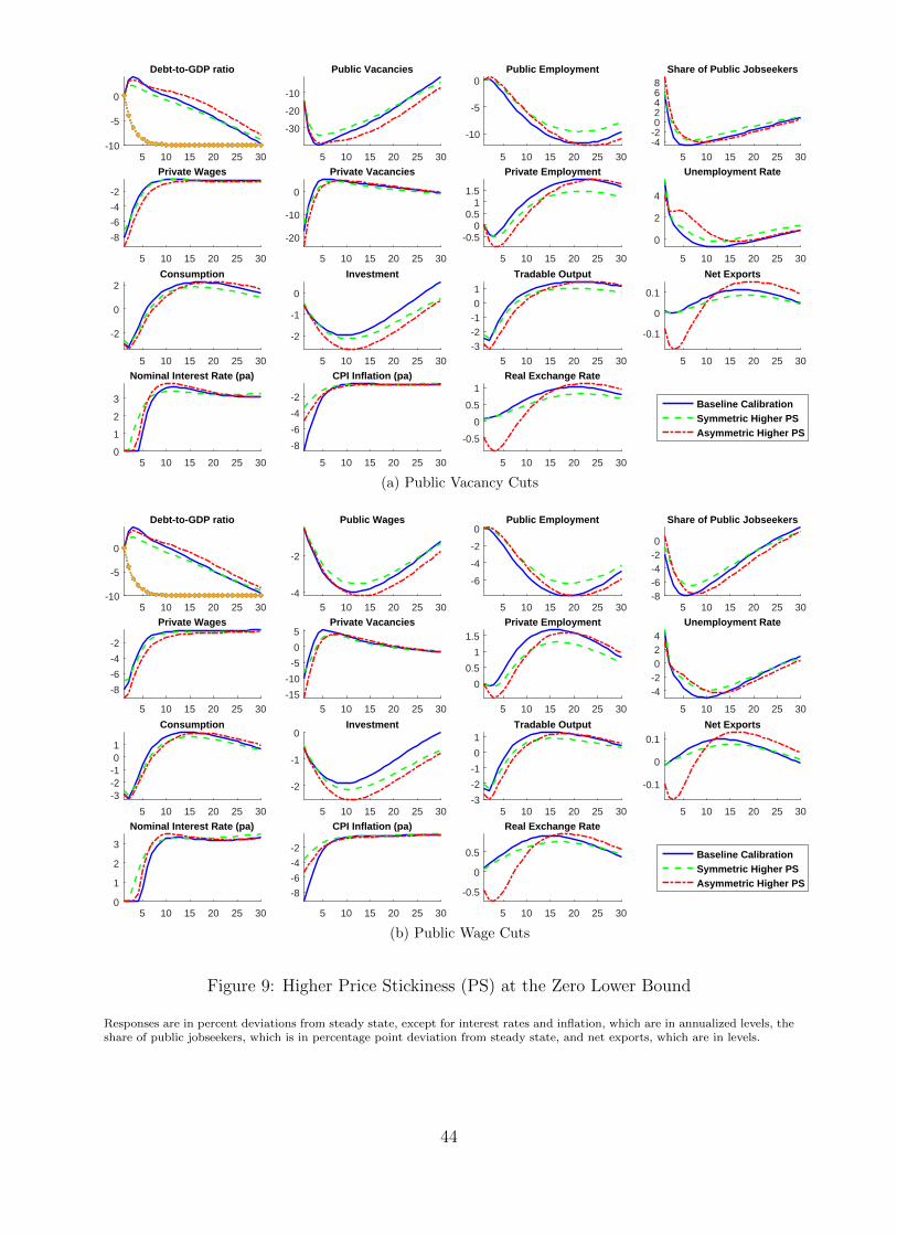
4.2 Price Rigidities

We have seen that fiscal consolidation through the public wage bill induces changes in relative

prices, which, under a fixed exchange rate regime, plays a role in the reallocation of resources

within the monetary union. This is particularly true at the ZLB, when monetary policy

cannot undo changes in relative prices induced by asymmetric fiscal shocks and, as a result,

the degree of price stickiness becomes important for the effects of fiscal consolidation.

The green dashed lines in Figures 9a and 9b depict the responses when we assume that

the degree of price rigidities increases for both regions by setting χ = 0.85. It is clear that

price rigidities matter for the success of the consolidation at the ZLB. The larger the share

of firms that cannot change their prices on impact, the weaker the negative effects of the

demand shocks on inflation and the milder the necessary consolidation. However, this result

is reversed when the degree of price stickiness is asymmetric between member states. The red

dotted lines in Figures 9a and 9b depict the responses when we assume that the degree of price

rigidities increases only in the Periphery. In this case, consolidation effort decreases in the

short run as inflation moves less than in the benchmark model. Still, higher price stickiness in

the Periphery implies larger effects from the negative demand shocks. The relative inability

of prices to adjust in the Periphery induces a reversal of the internal devaluation, meaning

an appreciation of the real exchange rate, which significantly reduces net exports. This effect

is then mirrored in the response of tradable output and employment.16

Overall, a higher degree of price rigidities in the Periphery implies an additional channel,

which operates through an appreciation of the real exchange rate, with adverse effects on net

16In the online appendix we show that asymmetries in wage stickiness, or in the mobility of jobseekers acrosssectors, are less important for our results. We also show that the degree of price stickiness is inconsequentialduring normal times, as monetary policy will always react to undo possible rigidities stemming from pricedispersion.

27

exports, output, private employment, and unemployment.

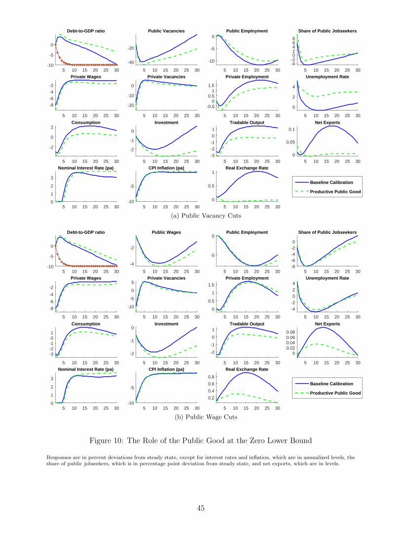
4.3 The Productivity of the Public Good

So far, we have assumed that the public good, ygt , does not play any role in the economy. As

an alternative, following Barro (1990) and Turnovsky (1999), we allow the public good, ygt ,

to enter the production function, taken as exogenous by the firms. To this end, we augment

the private production function to:

ypt = (npt )1−φ(xtk

pt )φ(ygt )

ν (40)

The parameter ν regulates how the public input affects private production: when ν is zero,

the government good is unproductive. This parameter is crucial in determining the effects

of consolidation, even in normal times. When ν > 0, fiscal consolidation in this environment

reduces the productive capacity of the firms by reducing the public good, and at the same

time induces a positive wealth effect, which raises private demand and therefore private labor

demand. Hence, ν is at the center of the balance between two opposite effects on private

production.

The green dashed lines in Figures 10a and 10b compare the responses of the baseline model

against the responses when we assume that ν = 0.15. When the public good is productive,

the reduction in the public wage bill implies a drop in the marginal product of labor, and this

leads to a bigger fall in private wages. For both instruments, there is a bigger contraction in

household consumption and investment, and ultimately a much larger and more persistent

drop in tradable output. In the case of vacancy cuts, where public employment, and hence

public output, falls more significantly, the differences are much starker. In this case, the

reallocation of jobseekers towards the private sector in the medium to long run is smaller,

since the expected return from working in the private sector is now smaller. Similarly,

the fact that the consolidation reduces the productivity of private jobs lowers the expected

returns from an additional hire for the firm, and, as a result, private vacancies fall more

in this case, inducing a bigger drop in private employment. More specifically, the initial

drop in private employment is larger and its subsequent evolution is always below baseline,

28

raising the unemployment rate considerably and persistently. With public wage cuts, since

public employment does not fall by as much when compared to the case of vacancy cuts,

this channel of amplification through the productivity of the public good is less important.

The fact that the consolidation decreases private productivity also implies that there is no

internal devaluation after vacancy cuts: the real exchange rate even appreciates after the

liquidity trap.17

In summary, when the public good is productive, there is a bigger fall in the private

wage, consumption, investment, and tradable output. For vacancy cuts, the impact on the

responses of private employment and the unemployment rate is more pronounced.

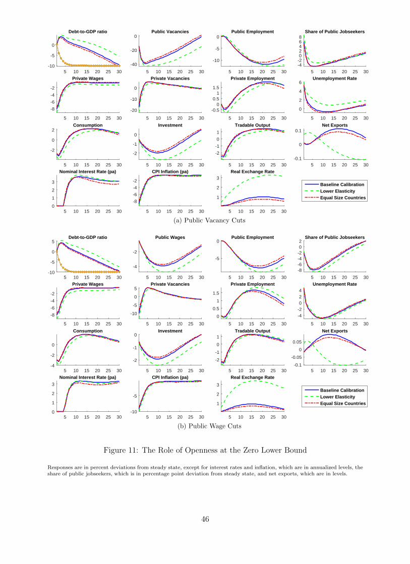
4.4 Particularities of the Open Economy

In this section we explore the open economy dimension of the model, in particular investigat-

ing the sensitivity of our findings to changes in the degree of trade elasticity and the relative

size of the member country implementing consolidation within the monetary union.

4.4.1 Elasticity of Trade

There is no strong consensus from the empirical literature regarding the value of the elasticity

of substitution between home-produced and imported goods, γ. Some recent contributions

have suggested low values for this parameter, in some cases with estimates well below one.

The green dashed lines in Figures 11a and 11b show the IRFs for the case when this elasticity

is reduced from 1.5 to 0.5, implying complementarity between traded goods.

With the foreign and domestic goods as complements, the internal devaluation no longer

leads to a substitution of both domestic and foreign demand towards the domestically pro-

duced good. Instead, it contracts demand for both types of goods in the Periphery. The

fall in domestic demand produces a larger fall in domestic inflation, resulting in a bigger

exchange rate depreciation and a larger rise in net exports.18 The deflationary pressures

17In results we present in the online appendix we show that assuming that the public good provides utilityto the households by being a substitute of private consumption does not significantly affect our baselineresults.

18The results of the fall in domestic demand are clearly illustrated in the online appendix where we plotthe sensitivity of results to changes in the trade elasticity in normal times. For a lower elasticity of trade,consumption and investment fall after the consolidation since agents cannot substitute domestic for foreign

29

increase the debt burden, rendering consolidation more difficult to achieve and increasing its

associated costs. Note in particular that, for vacancy cuts, the unemployment rate increases

significantly when domestic and foreign goods are assumed to be complements.

In conclusion, complementarity between home-produced and imported goods implies that

the deflationary pressures increase the debt burden, rendering consolidation more costly.

4.4.2 The Relative Size of Member Countries

The red dash-dotted lines in Figures 11a and 11b show the implications of increasing the

size of the Periphery to 50% of the monetary union. Since we assume that net foreign assets

are zero in the steady state, increasing the size of the Periphery also implies reducing the

home bias in the Core.19 Hence the differences in the composition of CPI across regions are

smaller, CPI differentials are reduced and this dampens the adjustment of the real exchange

rate. Furthermore, although final good producers in the Periphery still substitute between

domestic and foreign retail goods, their demand now represents a bigger share of total demand

for foreign goods and, therefore, affects foreign prices more. In the short to medium run, this

benefits firms in the Periphery, and it translates to a slightly smaller adjustment in private

demand, particularly in investment. This, in turn, helps the consolidation effort and reduces

the adjustment of both fiscal instruments required to meet the debt target.

Hence, we conclude that it is easier to consolidate for larger countries in a monetary

union, although the associated relative differences are small.

5 Conclusions

5.1 Summary

In this paper, we have set up a DSGE model of a monetary union with search and matching

frictions, nominal rigidities, and public employment, to study the effects of fiscal consolidation

through cuts in the public wage bill in a low inflation environment. Our model allows us

to study non-trivial reallocation of agents both in and out of the labor force and between

goods and this results in downward pressures on inflation.19For n = 0.5 and $ = 0.85, we have $? = 0.85

30

the public and private sector. In normal times, a reduction in the government wage bill

induces a reallocation of labor towards the private sector, due to the contraction in the

public sector, and so pushes down on private wages in the medium run. This leads to an

internal devaluation within the monetary union, which, along with the positive wealth effect

from the cut in government expenditure, raises aggregate demand and so implies an expansion

in the private sector.

In a low inflation environment, induced by negative demand shocks, the debt-to-GDP

ratio rises, and so larger fiscal cuts are needed to lower this ratio. Given the expansionary

effects this has for the private sector, consolidation helps the recovery of the economy in a

liquidity trap in the medium to long run. Nonetheless, with the contraction in demand, the

private sector is much more limited in its ability to absorb the workers leaving the public

sector, and so the expansionary effects of the consolidation are contained. On the other hand,

the effects of consolidation on the unemployment rate depend on the fiscal instrument used

at the ZLB: while public wage cuts quickly and effectively reduce the unemployment rate,

public vacancy cuts lead to a significant and more persistent rise in the unemployment rate.

5.2 Policy Implications

Our findings can be used as a roadmap for successful fiscal consolidations through cuts in

the public wage bill. First, since vacancy cuts have indirect and lagged effects on the dy-

namics of the private wage and no effects for the public wage, they could be more easily

implemented. In normal times, they also decrease unemployment relative to wage cuts and,

moreover, generate more persistent increases in employment, output and net exports. Clearly,

in terms of implementability but also long run effects, consolidating through vacancy cuts in

normal times presents certain advantages. At the ZLB, the two instruments deliver similar

outcomes apart from unemployment that decreases for wage cuts and remains high for va-

cancy cuts. This creates a trade-off for policy makers that must strike a balance between the

easier implementation of unfavourable policies using vacancy cuts, or controlling the rise in

unemployment due to the negative demand shocks using wage cuts.

We point to several factors that matter for the recovery from the low inflation environ-

31

ment. The most important are rigidities in the mobility of unemployed jobseekers between

the public and private sectors and nominal price stickiness. Rigidities in the reallocation of

workers between the two sectors make consolidation through cuts in the public wage bill more

adverse and come at the cost of higher unemployment in the medium to long run. Hence,

the presence of active labor market policies that can help channel workers from the public to

the private sector are crucial for the success of fiscal consolidations like the ones considered

in this paper. In a similar sense, relative price rigidities are also important: higher price

stickiness in the Periphery reverses the internal devaluation and leads instead to an appre-

ciation of the real exchange rate, which reinforces the negative effects of the demand shocks

and makes consolidation harder to achieve. Also in this case, structural reforms that reduce

those types of rigidities would ease consolidations in the Periphery. Furthermore, when the

public good which is being cut is a productive factor for the private sector, consolidation is

more difficult, since it reduces the marginal productivity of labor. This pushes down both on

firm’s demand for labor and household’s supply of labor in the private sector, and results in

a drag on the economy. Thus, policymakers should consider not only the number, but also

the quality, of workers when cutting jobs, and the sector in which pay cuts are implemented.

Also, we have compared consolidations through the public wage bill with traditional

instruments of fiscal consolidation considered in the existing literature, like tax hikes or

government consumption cuts. Public wage cuts continue to offer certain advantages in

terms of a fast recovery of the private sector and a reduction in the unemployment rate.

Still in a low inflation environment, even such a consolidation policy, cannot fully undo the

negative effects of the demand shocks.

References

Albrecht, J., Robayo-Abril, M. and Vroman, S.: 2015, Public Sector Employment in an

Equilibrium Search and Matching Model, Manuscript .

Ardagna, S.: 2007, Fiscal policy in unionized labor markets, Journal of Economic Dynamics

and Control 31(5), 1498 – 1534.

32

Barro, R. J.: 1990, Government Spending in a Simple Model of Endogenous Growth, Journal

of Political Economy 98(5), S103–26.

Bermperoglou, D., Pappa, E. and Vella, E.: 2017, The government wage bill and private

activity, Journal of Economic Dynamics and Control 79, 21–47.

Bradley, J., Postel-Vinay, F. and Turon, H.: 2016, Public sector wage policy and labor market

equilibrium: a structural model, Journal of European Economic Association (forthcoming).

Bruckner, M. and Pappa, E.: 2012, Fiscal expansions, unemployment, and labor force par-

ticipation: theory and evidence, International Economic Review 53(4), 1205–1228.

Campolmi, A. and Gnocchi, S.: 2016, Labor market participation, unemployment and mon-

etary policy, Journal of Monetary Economics 79, 17–29.

Christiano, L., Eichenbaum, M. and Rebelo, S.: 2011, When Is the Government Spending

Multiplier Large?, Journal of Political Economy 119(1), 78–121.

Coenen, G., Erceg, C. J., Freedman, C., Furceri, D., Kumhof, M., Lalonde, R., ... and

Trabandt, M.: 2012, Effects of Fiscal Stimulus in Structural Models, American Economic

Journal: Macroeconomics 4(1), 22–68.

Correia, I., Farhi, E., Nicolini, J. and Teles, P.: 2013, Unconventional Fiscal Policy at the

Zero Bound, American Economic Review 103(4), 1172–1211.

De Long, J. and Summers, L.: 2012, Fiscal Policy in a Depressed Economy, Brookings Papers

on Economic Activity pp. 233–297.

Demekas, D. G. and Kontolemis, Z. G.: 2000, Government employment and wages and labour

market performance, Oxford Bulletin of Economics and Statistics 62(3), 391–415.

Eggertsson, G.: 2011, What Fiscal Policy is Effective at Zero Interest Rates?, NBER Macroe-

conomics Annual 2010 25, 59–112.

Erceg, C. and Linde, J.: 2013, Fiscal Consolidation in a Currency Union: Spending Cuts vs.

Tax Hikes, Journal of Economic Dynamics and Control 37(2), 422–445.

33

Gomes, P.: 2015, Optimal public sector wages, The Economic Journal 125(587), 1425–1451.

Guerrieri, L. and Iacoviello, M.: 2015, OccBin: A toolkit for solving dynamic models with

occasionally binding constraints easily, Journal of Monetary Economics 70(C), 22–38.

Holm-Hadulla, F., Kamath, K., Lamo, A., Perez, J. J. and Schuknecht, L.: 2010, Public

wages in the euro area: towards securing stability and competitiveness, ECB Occasional

Paper (112).

Ilzetzki, E., Mendoza, E. and Vegh, C.: 2013, How Big (Small?) Are Fiscal Multipliers?,

Journal of Monetary Economics 60(2), 239–254.

Jalil, A.: 2012, Comparing Tax and Spending Multipliers: It’s All About Controlling for

Monetary Policy, Available at SSRN 2139855 .

Krause, M. U. and Lubik, T. A.: 2007, The (ir) relevance of real wage rigidity in the new

keynesian model with search frictions, Journal of Monetary Economics 54(3), 706–727.

Kuvshinov, D., Muller, G. J. and Wolf, M.: 2016, Deleveraging, deflation and depreciation

in the euro area, European Economic Review 88, 42–66.

Lamo, A., Moral-Benito, E. and Perez, J. J.: 2016, Does slack influence public and private

labor market interactions?, Working Paper Series 1890, European Central Bank.

McManus, R., Ozkan, F. G. and Trzeciakiewicz, D.: 2014, Self-defeating austerity at the zero

lower bound, Department of Economics, University of York .

Monacelli, T., Perotti, R. and Trigari, A.: 2010, Unemployment fiscal multipliers, Journal of

Monetary Economics 57, 531–553.

Moyen, S., Stahler, N. and Winkler, F.: 2016, Optimal Unemployment Insurance and In-

ternational Risk Sharing, Finance and Economics Discussion Series 2016-054, Board of

Governors of the Federal Reserve System.

Neiss, K. S. and Pappa, E.: 2005, Persistence without too much price stickiness: the role of

variable factor utilization, Review of Economic Dynamics 8(1), 231–255.

34

Pappa, E., Sajedi, R. and Vella, E.: 2015, Fiscal Consolidation with Tax Evasion and Cor-

ruption, Journal of International Economics 96(S1), 56–75.

Perez, J. J., Aouriri, M., Campos, M. M., Celov, D., Depalo, D., Papapetrou, E., Pesliakaite,

J., Ramos, R. and Rodrıguez-Vives, M.: 2016, The fiscal and macroeconomic effects of

government wages and employment reform, Occasional Papers 1607, Banco de Espana.

Quadrini, V. and Trigari, A.: 2007, Public employment and the business cycle, The Scandi-

navian Journal of Economics 109(4), 723–742.

Ravn, M.: 2008, The consumption-tightness puzzle, NBER International Seminar on

Macroeconomics 2006 pp. 9–63.

Reinhart, C., Reinhart, V. and Rogoff, K.: 2015, Dealing with Debt, Journal of International

Economics 96(S1), 43–55.

Rendahl, P.: 2016, Fiscal Policy in an Unemployment Crisis, Review of Economic Studies

83(3), 1189–1224.

Turnovsky, S. J.: 1999, Productive government expenditure in a stochastically growing econ-

omy, Macroeconomic Dynamics 3, 544–570.

Figures

35

2009 2010 2011 2012 2013

70

80

90

100

110

BE DE FR NL AT FI IE GR ES IT PT

Figure 1: Evolution of the Public Wage Bill

Wages and salaries in the public sector, current prices. For comparability, country series have beennormalized to 100 in 2009. Source: Eurostat and authors’ calculations.

36

-15

-10

-5

0

5

10

IE GR ES IT PT

% YoY

2009 2010 2011 2012 2013

(a) Average Wage per Employee

-7

-6

-5

-4

-3

-2

-1

0

1

2

3

IE GR ES IT PT

% YoY

2009 2010 2011 2012 2013

(b) Employment

Figure 2: Changes in Public Sector Wages and Employment

Source: Eurostat and authors’ calculations.

37

510

1520

2530

-10-50

Deb

t-to

-GD

P r

atio

510

1520

2530

-30

-20

-100

Fis

cal I

nst

rum

ent

510

1520

2530

-10-50

Pu

blic

Wag

e B

ill

510

1520

2530

-10-50

Pu

blic

Em

plo

ymen

t

510

1520

2530

-6-4-20

Sh

are

of

Pu

blic

Jo

bse

eker

s

510

1520

2530

-0.50

0.5

Pri

vate

Wag

es

510

1520

2530

-202468P

riva

te V

acan

cies

510

1520

2530

012P

riva

te E

mp

loym

ent

510

1520

2530

0

0.51

1.5

Co

nsu

mp

tio

n

510

1520

2530

012

Inve

stm

ent

510

1520

2530

0

0.51

1.5

Tra

dab

le O

utp

ut

510

1520

2530

-0.20

0.2

Rea

l GD

P

510

1520

2530

-4-20

Un

emp

loym

ent

Rat

e

510

1520

2530

-0.3

-0.2

-0.1

Lab

or

Par

tici

pat

ion

Rat

e

510

1520

2530

0

0.050.1

Net

Exp

ort

s

510

1520

2530

-0.20

0.2

0.4

0.6

0.8

Rea

l Exc

han

ge

Rat

e

510

1520

2530

3.54

4.5

No

min

al In

tere

st R

ate

(pa)

510

1520

2530

-0.20

0.2

0.4

CP

I In

flat

ion

(p

a)

510

1520

2530

3.84

4.2

4.4

4.6

Rea

l In

tere

st R

ate

(pa)

Vac

ancy

Cu

tsW

age

Cu

tsS

pen

din

g C

uts

Tax

Hik

es

Fig

ure

3:N

orm

alT

imes

:C

ompar

ison

ofF

isca

lIn

stru

men

ts

Res

pon

ses

are

inp

erce

nt

dev

iati

ons

from

stea

dy

stat

e,ex

cep

tfo

rin

tere

stra

tes

an

din

flati

on

,w

hic

hare

inan

nu

ali

zed

leve

ls,

the

share

of

pu

bli

cjo

bse

eker

s,w

hic

his

inp

erce

nta

gep

oint

dev

iati

onfr

omst

ead

yst

ate,

and

net

exp

ort

s,w

hic

hare

inle

vel

s.

38

510

1520

2530

-10-50

Deb

t-to

-GD

P r

atio

510

1520

2530

-30

-20

-100

Pu

blic

Vac

anci

es

510

1520

2530

-10-50

Pu

blic

Wag

e B

ill

510

1520

2530

-10-50

Pu

blic

Em

plo

ymen

t

510

1520

2530

-4-2024

Sh

are

of

Pu

blic

Jo

bse

eker

s

510

1520

2530

-8-6-4-20P

riva

te W

ages

510

1520

2530

-15

-10-505

Pri

vate

Vac

anci

es

510

1520

2530

012P

riva

te E

mp

loym

ent

510

1520

2530

-202C

on

sum

pti

on

510

1520

2530

-1012

Inve

stm

ent

510

1520

2530

-2-101

Tra

dab

le O

utp

ut

510

1520

2530

-2-10R

eal G

DP

510

1520

2530

0246U

nem

plo

ymen

t R

ate

510

1520

2530

-0.20

0.2

0.4

Lab

or

Par

tici

pat

ion

Rat

e

510

1520

2530

0

0.050.1

Net

Exp

ort

s

510

1520

2530

0.2

0.4

0.6

0.81

Rea

l Exc

han

ge

Rat

e

510

1520

2530

-6-4-2024N

om

inal

Inte

rest

Rat

e (p

a)

510

1520

2530

-8-6-4-20C

PI I

nfl

atio

n (

pa)

510

1520

2530

0246

Rea

l In

tere

st R

ate

(pa)

No

rmal

Tim

esL

ow

Infl

atio

n:

un

con

stra

ined

Lo

w In

flat

ion

: co

nst

rain

ed b

y Z

LB

Fig

ure

4:N

orm

alT

imes

vs.

Low

Inflat

ion

Envir

onm

ent:

Public

Vac

ancy

Cuts

Res

pon

ses

are

inp

erce

nt

dev

iati

ons

from

stea

dy

stat

e,ex

cep

tfo

rin

tere

stra

tes

an

din

flati

on

,w

hic

hare

inan

nu

ali

zed

leve

ls,

the

share

of

pu

bli

cjo

bse

eker

s,w

hic

his

inp

erce

nta

gep

oint

dev

iati

onfr

omst

ead

yst

ate,

and

net

exp

ort

s,w

hic

hare

inle

vel

s.

39

510

1520

2530

-10-50

Deb

t-to

-GD

P r

atio

510

1520

2530

-3-2-1

Pu

blic

Wag

es

510

1520

2530

-10-8-6-4-2

Pu

blic

Wag

e B

ill

510

1520

2530

-50P

ub

lic E

mp

loym

ent

510

1520

2530

-8-6-4-20

Sh

are

of

Pu

blic

Jo

bse

eker

s

510

1520

2530

-8-6-4-20P

riva

te W

ages

510

1520

2530

-505

Pri

vate

Vac

anci

es

510

1520

2530

0

0.51

1.5

Pri

vate

Em

plo

ymen

t

510

1520

2530

-3-2-101

Co

nsu

mp

tio

n

510

1520

2530

-1012In

vest

men

t

510

1520

2530

-2-101

Tra

dab

le O

utp

ut

510

1520

2530

-2-10

Rea

l GD

P

510

1520

2530

-4-2024

Un

emp

loym

ent

Rat

e

510

1520

2530

-0.20

0.2

0.4

Lab

or

Par

tici

pat

ion

Rat

e

510

1520

2530

-0.0

200.

020.

040.

060.

08

Net

Exp

ort

s

510

1520

2530

0.2

0.4

0.6

0.8

Rea

l Exc

han

ge

Rat

e

510

1520

2530

-6-4-2024N

om

inal

Inte

rest

Rat

e (p

a)

510

1520

2530

-8-6-4-20C

PI I

nfl

atio

n (

pa)

510

1520

2530

0246

Rea

l In

tere

st R

ate

(pa)

No

rmal

Tim

esL

ow

Infl

atio

n:

un

con

stra

ined

Lo

w In

flat

ion

: co

nst

rain

ed b

y Z

LB

Fig

ure

5:N

orm

alT

imes

vs.

Low

Inflat

ion

Envir

onm

ent:

Public

Wag

eC

uts

Res

pon

ses

are

inp

erce

nt

dev

iati

ons

from

stea

dy

stat

e,ex

cep

tfo

rin

tere

stra

tes

an

din

flati

on

,w

hic

hare

inan

nu

ali

zed

leve

ls,

the

share

of

pu

bli

cjo

bse

eker

s,w

hic

his

inp

erce

nta

gep

oint

dev

iati

onfr

omst

ead

yst

ate,

and

net

exp

ort

s,w

hic

hare

inle

vel

s.

40

510

1520

2530

-10-505

Deb

t-to

-GD

P r

atio

510

1520

2530

-30

-20

-100

Fis

cal I

nst

rum

ent

510

1520

2530

-10-50

Pu

blic

Wag

e B

ill

510

1520

2530

-10-50

Pu

blic

Em

plo

ymen

t

510

1520

2530

-505

Sh

are

of

Pu

blic

Jo

bse

eker

s

510

1520

2530

-10-50

Pri

vate

Wag

es

510

1520

2530

-20

-100

Pri

vate

Vac

anci

es

510

1520

2530

-101

Pri

vate

Em

plo

ymen

t

510

1520

2530

-4-202C

on

sum

pti

on

510

1520

2530

-3-2-10

Inve

stm

ent

510

1520

2530

-3-2-101

Tra

dab

le O

utp

ut

510

1520

2530

-2.5-2

-1.5-1

-0.5

Rea

l GD

P

510

1520

2530

-4-2024

Un

emp

loym

ent

Rat

e

510

1520

2530

-0.4

-0.20

0.2

0.4

Lab

or

Par

tici

pat

ion

Rat

e

510

1520

2530

0

0.050.1

Net

Exp

ort

s

510

1520

2530

0

0.51

Rea

l Exc

han

ge

Rat

e

510

1520

2530

0123

No

min

al In

tere

st R

ate

(pa)

510

1520

2530

-10-8-6-4-2

CP

I In

flat

ion

(p

a)

510

1520

2530

2468R

eal I

nte

rest

Rat

e (p

a)

Vac

ancy

Cu

tsW

age

Cu

tsS

pen

din

g C

uts

Tax

Hik

es

Fig

ure

6:L

owIn

flat

ion

Envir

onm

ent:

Com

par

ison

ofF

isca

lIn

stru

men

ts

Res

pon

ses

are

inp

erce

nt

dev

iati

ons

from

stea

dy

stat

e,ex

cep

tfo

rin

tere

stra

tes

an

din

flati

on

,w

hic

hare

inan

nu

ali

zed

leve

ls,

the

share

of

pu

bli

cjo

bse

eker

s,w

hic

his

inp

erce

nta

gep

oint

dev

iati

onfr

omst

ead

yst

ate,

and

net

exp

ort

s,w

hic

hare

inle

vel

s.

41

5 10 15 20 25 30-10

-5

0

Debt-to-GDP ratio

5 10 15 20 25 30

-30

-20

-10

Public Vacancies

5 10 15 20 25 30

-10

-5

0Public Employment

5 10 15 20 25 30

-4-202468

Share of Public Jobseekers

5 10 15 20 25 30

-8

-6

-4

-2

Private Wages

5 10 15 20 25 30

-20

-10

0

Private Vacancies

5 10 15 20 25 30

-0.50

0.51

1.5

Private Employment

5 10 15 20 25 30

0

2

4

Unemployment Rate

5 10 15 20 25 30

-2

0

2Consumption

5 10 15 20 25 30

-2

-1

0

Investment

5 10 15 20 25 30-3

-2

-1

0

1

Tradable Output

5 10 15 20 25 30

0

0.05

0.1

Net Exports

5 10 15 20 25 300

1

2

3

Nominal Interest Rate (pa)

5 10 15 20 25 30

-8-6-4-2

CPI Inflation (pa)

5 10 15 20 25 30

0.5

1Real Exchange Rate

Consolidation Shock

No Consolidation Shock

(a) Public Vacancy Cuts.

5 10 15 20 25 30-10

-5

0

Debt-to-GDP ratio

5 10 15 20 25 30

-3

-2

-1

Public Wages

5 10 15 20 25 30

-6

-4

-2

0

Public Employment

5 10 15 20 25 30

-5

0

5Share of Public Jobseekers

5 10 15 20 25 30

-8

-6

-4

-2

Private Wages

5 10 15 20 25 30

-15-10-505

Private Vacancies

5 10 15 20 25 30

-0.50

0.51

1.5Private Employment

5 10 15 20 25 30

-4-2024

Unemployment Rate

5 10 15 20 25 30

-3-2-101

Consumption

5 10 15 20 25 30

-2

-1

0Investment

5 10 15 20 25 30

-2

-1

0

1Tradable Output

5 10 15 20 25 30

00.020.040.060.08

Net Exports

5 10 15 20 25 300

1

2

3

Nominal Interest Rate (pa)

5 10 15 20 25 30

-8-6-4-2

CPI Inflation (pa)

5 10 15 20 25 30

0.2

0.4

0.6

0.8

Real Exchange Rate

Consolidation Shock

No Consolidation Shock

(b) Public Wage Cuts

Figure 7: The Role of Consolidation at the Zero Lower Bound

Responses are in percent deviations from steady state, except for interest rates and inflation, which are in annualized levels, theshare of public jobseekers, which is in percentage point deviation from steady state, and net exports, which are in levels.

42

5 10 15 20 25 30-10

-5

0

5Debt-to-GDP ratio

5 10 15 20 25 30

-40

-20

Public Vacancies

Baseline Calibration

Fixed Share of Jobseekers

5 10 15 20 25 30

-10

-5

0Public Employment

5 10 15 20 25 30

-4-2024

Share of Public Jobseekers

5 10 15 20 25 30

-8

-6

-4

-2

Private Wages

5 10 15 20 25 30

-15

-10

-5

0

5Private Vacancies

5 10 15 20 25 30

00.5

11.5

Private Employment

5 10 15 20 25 30

0

2

4

6Unemployment Rate

5 10 15 20 25 30

-2

0

2Consumption

5 10 15 20 25 30

-2

-1

0

Investment

5 10 15 20 25 30

-2

-1

0

1

Tradable Output

5 10 15 20 25 300

0.05

0.1

Net Exports

5 10 15 20 25 300

1

2

3

Nominal Interest Rate (pa)

5 10 15 20 25 30

-10-8-6-4-2

CPI Inflation (pa)

5 10 15 20 25 30

0.5

1Real Exchange Rate

(a) Public Vacancy Cuts

5 10 15 20 25 30-10

-5

0

5Debt-to-GDP ratio

5 10 15 20 25 30

-4

-2

Public Wages

Baseline Calibration

Fixed Share of Jobseekers

5 10 15 20 25 30

-6

-4

-2

0Public Employment

5 10 15 20 25 30-8-6-4-20

Share of Public Jobseekers

5 10 15 20 25 30

-8

-6

-4

-2

Private Wages

5 10 15 20 25 30

-5

0

5Private Vacancies

5 10 15 20 25 30

0

0.5

1

1.5

Private Employment

5 10 15 20 25 30

-4-2024

Unemployment Rate

5 10 15 20 25 30-4

-2

0

Consumption

5 10 15 20 25 30

-2

-1

0Investment

5 10 15 20 25 30

-2

-1

0

1Tradable Output

5 10 15 20 25 30

00.020.040.060.08

Net Exports

5 10 15 20 25 300

1

2

3

Nominal Interest Rate (pa)

5 10 15 20 25 30

-10-8-6-4-2

CPI Inflation (pa)

5 10 15 20 25 30

0.2

0.4

0.6

0.8

Real Exchange Rate

(b) Public Wage Cuts

Figure 8: Labor Market Rigidities at the Zero Lower Bound

Responses are in percent deviations from steady state, except for interest rates and inflation, which are in annualized levels, theshare of public jobseekers, which is in percentage point deviation from steady state, and net exports, which are in levels.

43

5 10 15 20 25 30-10

-5

0

Debt-to-GDP ratio

5 10 15 20 25 30

-30

-20

-10

Public Vacancies

Baseline CalibrationSymmetric Higher PSAsymmetric Higher PS

5 10 15 20 25 30

-10

-5

0Public Employment

5 10 15 20 25 30-4-202468

Share of Public Jobseekers

5 10 15 20 25 30

-8

-6

-4

-2

Private Wages

5 10 15 20 25 30

-20

-10

0

Private Vacancies

5 10 15 20 25 30

-0.50

0.51

1.5

Private Employment

5 10 15 20 25 30

0

2

4

Unemployment Rate

5 10 15 20 25 30

-2

0

2Consumption

5 10 15 20 25 30

-2

-1

0

Investment

5 10 15 20 25 30

-3-2-101

Tradable Output

5 10 15 20 25 30

-0.1

0

0.1

Net Exports

5 10 15 20 25 300

1

2

3

Nominal Interest Rate (pa)

5 10 15 20 25 30

-8

-6

-4

-2

CPI Inflation (pa)

5 10 15 20 25 30

-0.5

0

0.5

1Real Exchange Rate

(a) Public Vacancy Cuts

5 10 15 20 25 30-10

-5

0

Debt-to-GDP ratio

5 10 15 20 25 30-4

-2

Public Wages

Baseline CalibrationSymmetric Higher PSAsymmetric Higher PS

5 10 15 20 25 30

-6

-4

-2

0Public Employment

5 10 15 20 25 30-8-6-4-20

Share of Public Jobseekers

5 10 15 20 25 30

-8

-6

-4

-2

Private Wages

5 10 15 20 25 30-15

-10

-5

0

5Private Vacancies

5 10 15 20 25 30

0

0.5

1

1.5Private Employment

5 10 15 20 25 30

-4-2024

Unemployment Rate

5 10 15 20 25 30

-3-2-101

Consumption

5 10 15 20 25 30

-2

-1

0Investment

5 10 15 20 25 30-3

-2

-1

0

1Tradable Output

5 10 15 20 25 30

-0.1

0

0.1

Net Exports

5 10 15 20 25 300

1

2

3

Nominal Interest Rate (pa)

5 10 15 20 25 30

-8

-6

-4

-2

CPI Inflation (pa)

5 10 15 20 25 30

-0.5

0

0.5

Real Exchange Rate

(b) Public Wage Cuts

Figure 9: Higher Price Stickiness (PS) at the Zero Lower Bound

Responses are in percent deviations from steady state, except for interest rates and inflation, which are in annualized levels, theshare of public jobseekers, which is in percentage point deviation from steady state, and net exports, which are in levels.

44

5 10 15 20 25 30-10

-5

0

Debt-to-GDP ratio

5 10 15 20 25 30

-40

-20

Public Vacancies

Baseline Calibration

Productive Public Good

5 10 15 20 25 30

-10

-5

0Public Employment

5 10 15 20 25 30-4-202468

Share of Public Jobseekers

5 10 15 20 25 30

-8

-6

-4

-2

Private Wages

5 10 15 20 25 30

-20

-10

0

Private Vacancies

5 10 15 20 25 30

-0.50

0.51

1.5

Private Employment

5 10 15 20 25 30

0

2

4

Unemployment Rate

5 10 15 20 25 30

-2

0

2Consumption

5 10 15 20 25 30

-2

-1

0

Investment

5 10 15 20 25 30-3

-2

-1

0

1

Tradable Output

5 10 15 20 25 30

0

0.05

0.1

Net Exports

5 10 15 20 25 300

1

2

3

Nominal Interest Rate (pa)

5 10 15 20 25 30-10

-5

CPI Inflation (pa)

5 10 15 20 25 30

0

0.5

1Real Exchange Rate

(a) Public Vacancy Cuts

5 10 15 20 25 30-10

-5

0

Debt-to-GDP ratio

5 10 15 20 25 30

-4

-2

Public Wages

Baseline Calibration

Productive Public Good

5 10 15 20 25 30

-5

0Public Employment

5 10 15 20 25 30-8-6-4-20

Share of Public Jobseekers

5 10 15 20 25 30

-8

-6

-4

-2

Private Wages

5 10 15 20 25 30

-10

-5

0

5Private Vacancies

5 10 15 20 25 30

0

0.5

1

1.5

Private Employment

5 10 15 20 25 30

-4-2024

Unemployment Rate

5 10 15 20 25 30

-3-2-101

Consumption

5 10 15 20 25 30

-2

-1

0Investment

5 10 15 20 25 30

-2

-1

0

1Tradable Output

5 10 15 20 25 30

00.020.040.060.08

Net Exports

5 10 15 20 25 300

1

2

3

Nominal Interest Rate (pa)

5 10 15 20 25 30-10

-5

CPI Inflation (pa)

5 10 15 20 25 30

0.2

0.4

0.6

0.8

Real Exchange Rate

(b) Public Wage Cuts

Figure 10: The Role of the Public Good at the Zero Lower Bound

Responses are in percent deviations from steady state, except for interest rates and inflation, which are in annualized levels, theshare of public jobseekers, which is in percentage point deviation from steady state, and net exports, which are in levels.

45

5 10 15 20 25 30-10

-5

0

Debt-to-GDP ratio

5 10 15 20 25 30

-40

-20

0Public Vacancies

Baseline CalibrationLower ElasticityEqual Size Countries

5 10 15 20 25 30

-10

-5

0Public Employment

5 10 15 20 25 30

-4-202468

Share of Public Jobseekers

5 10 15 20 25 30

-8

-6

-4

-2

Private Wages

5 10 15 20 25 30

-20

-10

0

Private Vacancies

5 10 15 20 25 30

-0.50

0.51

1.5

Private Employment

5 10 15 20 25 30

0

2

4

6Unemployment Rate

5 10 15 20 25 30

-2

0

2Consumption

5 10 15 20 25 30

-2

-1

0

Investment

5 10 15 20 25 30

-2

-1

0

1

Tradable Output

5 10 15 20 25 30-0.1

0

0.1Net Exports

5 10 15 20 25 300

1

2

3

Nominal Interest Rate (pa)

5 10 15 20 25 30

-8

-6

-4

-2

CPI Inflation (pa)

5 10 15 20 25 30

1

2

3Real Exchange Rate

(a) Public Vacancy Cuts

5 10 15 20 25 30-10

-5

0

5Debt-to-GDP ratio

5 10 15 20 25 30

-4

-2

Public Wages

Baseline CalibrationLower ElasticityEqual Size Countries

5 10 15 20 25 30

-5

0Public Employment

5 10 15 20 25 30

-8-6-4-202

Share of Public Jobseekers

5 10 15 20 25 30

-8

-6

-4

-2

Private Wages

5 10 15 20 25 30

-10

-5

0

5Private Vacancies

5 10 15 20 25 30

0

0.5

1

1.5

Private Employment

5 10 15 20 25 30

-4-2024

Unemployment Rate

5 10 15 20 25 30-4

-2

0

Consumption

5 10 15 20 25 30

-2

-1

0Investment

5 10 15 20 25 30

-2

-1

0

1Tradable Output

5 10 15 20 25 30-0.1

-0.05

0

0.05

Net Exports

5 10 15 20 25 300

1

2

3

Nominal Interest Rate (pa)

5 10 15 20 25 30-10

-5

CPI Inflation (pa)

5 10 15 20 25 30

1

2

3

Real Exchange Rate

(b) Public Wage Cuts

Figure 11: The Role of Openness at the Zero Lower Bound

Responses are in percent deviations from steady state, except for interest rates and inflation, which are in annualized levels, theshare of public jobseekers, which is in percentage point deviation from steady state, and net exports, which are in levels.

46